Effective Medium Models - Stanford University Rock Physics Laboratory - Gary Mavko Effective Medium Theories 116 The Voigt and Reuss averages are interpreted as the ratio of average

Stanford Rock Physics Laboratory - Gary Mavko

Effective Medium Theories

113

Effective Medium Models



114

Bounding Methods for EstimatingEffective Elastic Moduli

For many reasons we would like to be able to modelor estimate the effective elastic moduli of rocks interms of the properties of the various constituentminerals and pore fluids. To do it precisely one mustincorporate

• the individual elastic moduli of the constituents

• the volume fractions of the constituents

• geometric details of how the various constituents

are arranged

The geometric details are the most difficult to know ormeasure. If we ignore (or don’t know) the details ofgeometry, then the best we can do is estimate upperand lower bounds on the moduli or velocities.

The bounds are powerful and robust tools. They giverigorous upper and lower limits on the moduli, giventhe composition. If you find that your measurementsfall outside the bounds, then you have made a mistake- in velocity, volume fractions, or composition!



115

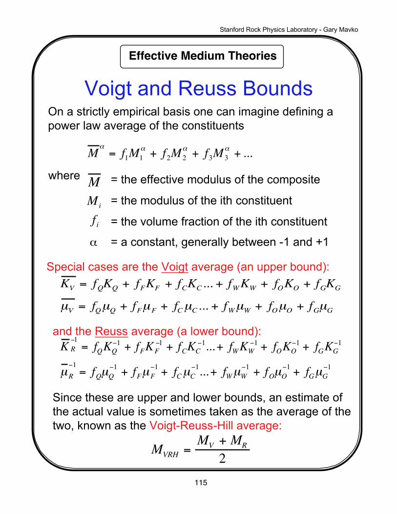
Voigt and Reuss BoundsOn a strictly empirical basis one can imagine defining apower law average of the constituents

where

Special cases are the Voigt average (an upper bound):

and the Reuss average (a lower bound):

Since these are upper and lower bounds, an estimate ofthe actual value is sometimes taken as the average of thetwo, known as the Voigt-Reuss-Hill average:

= the effective modulus of the composite

= the modulus of the ith constituent

= the volume fraction of the ith constituent

α = a constant, generally between -1 and +1

Mα= f1M1

α + f2M2α + f3M3

α + ...

KV = fQKQ + fFKF + fCKC ... + fWKW + fOKO + fGKG

µV = fQµQ + fFµF + fCµC ... + fWµW + fOµO + fGµG

K R−1

= fQKQ−1 + fFKF

−1 + fCKC−1...+ fWKW

−1 + fOKO−1 + fGKG

−1

µR−1

= fQµQ−1 + fFµF

−1 + fCµC−1...+ fWµW

−1 + fOµO−1 + fGµG

−1

M

MVRH =MV + MR

2

Mi

fi



116

The Voigt and Reuss averages are interpreted as the ratioof average stress and average strain within the composite.

The stress and strain are generally unknown in thecomposite and are expected to be nonuniform. The upperbound (Voigt) is found assuming that the strain iseverywhere uniform. The lower bound (Reuss) is foundassuming that the stress is everywhere uniform.

Geometric interpretations:

Voigt iso-strain model Reuss iso-stress model

Since the Reuss average describes an isostress situation,it applies perfectly to suspensions and fluid mixtures.

ˆ E =ˆ σ ˆ ε

=fiσ i∑ˆ ε

=fi( ˆ ε Ei)∑

ˆ ε ˆ E =

ˆ σ ˆ ε

=ˆ σ fiεi∑

=ˆ σ

fi(ˆ σ

Ei)∑

1ˆ E

=fi

Ei∑ˆ E = fi∑ Ei



117

Velocity-porosity relationship in clastic sediments compared withthe Voigt and Reuss bounds. Virtually all of the points indeedfall between the bounds. Furthermore, the suspensions, whichare isostress materials (points with porosity > 40%) fall veryclose to the Reuss bound.

Data from Hamilton (1956), Yin et al. (1988), Han et al. (1986). Compiled byMarion, D., 1990, Ph.D. dissertation, Stanford Univ.



118

Hashin-Shtrikman Bounds

Interpretation of bulk modulus:

where subscript 1 = shell, 2 = sphere. f1 and f2 are volumefractions.

These give upper bounds when stiff material is K1, µ1 (shell)and lower bounds when soft material is K1, µ1.

The narrowest possible bounds on moduli that we canestimate for an isotropic material, knowing only the volumefractions of the constituents, are the Hashin-Shtrikmanbounds. (The Voigt-Reuss bounds are wider.) For a mixtureof 2 materials:

K HS ± = K1 +f2

K2 − K1( )−1+ f1 K1 +

4

3µ1

−1

µ HS± = µ1 +f2

µ 2 − µ1( )−1+

2 f1(K1 + 2µ1)

5µ1 K1 +4

3µ1



119

Hashin-Shtrikman Bounds

A more general form that applies when more thantwo phases are being mixed (Berryman, 1993):

where

indicates volume average over the spatiallyvarying K(r), µ(r) of the constituents.

K HS + = Λ(µmax), K HS− = Λ(µmin)

µ HS+ = Γ ζ Kmax,,µmax( )( ), µHS − = Γ ζ Kmin ,µmin( )( )

Λ(z) =1

K(r) +43z

−1

−43z

Γ(z) =1

µ(r) + z

−1

− z

ζ(K ,µ) =µ69K + 8µK + 2µ



120

Here we see that a mixture of calcite and water giveswidely spaced bounds, but a mixture of calcite anddolomite gives very narrow bounds.

G13

Distance between bounds depends onsimilarity/difference of end-member constituents.



121

Wyllie Time Average

1

2

3

d1

d2

d3

D

Wyllie et al. (1956, 1958, 1962) found that travel timethrough water saturated consolidated rocks could beapproximately described as the volume weighted averageof the travel time through the constituents:

t =DV

t = t1 + t2 + t3DV

=d1V1

+d2V2

+d3V3

1V =

d1 /DV1

+d2 /DV2

+d3 /DV3

1V

=f1V1

+f2V2

+f3V3



122

Limitations:

• rock is isotropic• rock must be fluid-saturated• rock should be at high effective pressure• works best with primary porosity• works best at intermediate porosity• must be careful of mixed mineralogy (clay)

The time-average equation is heuristic andcannot be justified theoretically. It is based onray theory which requires that (1) thewavelength is smaller than the grain and poresize, and (2) the minerals and pores arearranged in flat layers.

Note the problem for shear waves where oneof the phases is a fluid, Vs-fluid → 0!

Wyllie’s generally works best for

• water-saturated rocks• consolidated rocks• high effective pressures



123

Modification of Wyllie's proposed by Raymer

Still a strictly empirical relation.

This relation recognizes that at large porosities (φ > 47%) thesediment behaves as a suspension, with the Reuss averageof the P-wave modulus, M = ρVp2.

V = (1− φ)2Vmineral + φVfluid1

ρV 2 =φ

ρfluidVfluid2+

1− φρmineralVmineral2

1V

=0.47 −φ0.10

1V37

+φ − 0.370.10

1V47

φ < 37%

φ > 47%

37% < φ < 47%



124

Comparison of Wyllie's time average equationand the Raymerequations with Marion's compilation of shaly-sand velocitiesfrom Hamilton (1956), Yin et al. (1988), Han et al. 1986).

G.3



125

Backus Average for Thinly Layered MediaBackus (1962) showed that in the long wavelength limit astratified medium made up of thin layers is effectivelyanisotropic. It becomes transversely isotropic, withsymmetry axis normal to the strata. The elastic constants(see next page) are given by:

where

are the isotropic elastic constants of the individuallayers. The brackets indicate averages of the enclosedproperties, weighted by their volumetric proportions. This isoften called the Backus average.

λ, µ

A =4µ(λ + µ)

λ + 2µ+

1λ + 2µ

−1λ

λ + 2µ

2

B =2µλ

λ + 2µ+

1λ + 2µ

−1λ

λ + 2µ

2

C =1

λ + 2µ

−1

F =1

λ + 2µ

−1λ

λ + 2µ

D =1µ

−1

M = µ

M =12 A− B( )

A B F 0 0 0B A F 0 0 0F F C 0 0 00 0 0 D 0 00 0 0 0 D 00 0 0 0 0 M



126

Hooke’s law relating stress and strain in a linear elasticmedium can be written as

elastic stiffnesses (moduli) elastic compliances

A standard shorthand is to write the stress and strain as vectors:

T =

σ 1= σ 11σ 2= σ 22σ 3= σ 33σ 4= σ 23σ 5= σ 13σ 6= σ 12

E =

e1= ε11e2= ε22e3= ε33e4=2ε23e5=2ε13e6=2ε12

σ 1σ 2σ 3σ 4σ 5σ 6

=

A B F 0 0 0B A F 0 0 0F F C 0 0 00 0 0 D 0 00 0 0 0 D 00 0 0 0 0 M

e1e2e3e4e5e6

Note the factor of 2 in the definition of strains.

The elastic constants are similarly written inabreviated form, and the Backus average constantsshown on the previous page now have the meaning:

σ ij = cijkl εklΣkl

ε ij = Sijkl σ klΣkl



127

Seismic Fluid Substitution

Pore fluids, pore stiffness,

and their interaction



128

Typical Problem: Analyze how rock properties, logs,and seismic change, when pore fluids change.

Example: We observe Vp, Vs, and density at a well and compute a synthetic seismic trace, as usual. Predict how the seismic will change if the fluid changes -- either over time at the same position, or if we move laterally away from the welland encounter different fluids in roughly the same rocks.



129

Effective moduli for specific pore and graingeometries

Imagine a single linear elastic body. We do two separateexperiments--apply stresses σ1 and observe displacementsu1, then apply stresses σ2 and observe displacements u2.

The Betti-Rayleigh reciprocity theorem states that the workdone by the first set of forces acting through the second setof displacements is equal to the work done by the secondset of forces acting through the first set of displacements.

σij(1), u(1)

∆σ

σij(2), u(2)

∆σ



130

Estimate of Dry Compressibility

Applying the reciprocity theorem we can write:

Assumptions • minerals behave elastically • friction and viscosity not important • assumes a single average mineral

limit as

∆σ

∆σ

∆σ

∆σ

∆σ

∆σ∆σVbulkKdry

− ∆σ∆Vpore =∆σ∆σVbulkKmineral

1Kdry

=1

Kmineral+1

Vbulk

∂Vpore∂σ

∆σ → 0



131

Relation of Rock Moduli to Pore Space Compressibility -- Dry Rock

where

G.4

A fairly general and rigorous relation between dry rock bulk modulus and porosity is

1K dry

= 1K mineral

+ φK φ

1

K φ= 1

vpore

∂vpore

∂σ

is the pore space stiffness. This is a new concept that quantifies the stiffness of a pore shape.

K φ



132

What is a “Dry Rock”?

Many rock models incorporate the concept of a dryrock or the dry rock frame. This includes the work byBiot, Gassmann, Kuster and Toksoz, etc, etc.

Caution: “Dry rock” is not the same as gas-saturatedrock. The dry frame modulus in these models refers to theincremental bulk deformation resulting from an increment ofapplied confining pressure, with pore pressure heldconstant. This corresponds to a “drained” experiment inwhich pore fluids can flow freely in or out of the sample toinsure constant pore pressure. Alternatively, it cancorrespond to an undrained experiment in which the porefluid has zero bulk modulus, so that pore compressions donot induce changes in pore pressure – this is approximatelythe case for an air-filled sample at standard temperature andpressure. However, at reservoir conditions (high porepressure), gas takes on a non-negligible bulk modulus, andshould be treated as a saturating fluid.



133

Relation of Rock Moduli to Pore Space Compressibility -- Saturated Rock

where Pore spacecompressibilitymodified by fluids.

A similar general relation between saturated rock bulk modulus and porosity is

1K sat

= 1K mineral

+ φK φ

K φ = K φ + K mineralK fluid

K mineral – K fluid ≈ K φ + K fluid

So we see that changing the pore fluid has the effect ofchanging the pore space compressibility of the rock. Thefluid modulus term is always just added to K φ

When we have a stiff rock with high velocity, then its valueof is large, and changes in do not have much effect.But a soft rock with small velocity will have a small and changes in will have a much larger effect.

K φ

K φ

K fluid

K fluid



134

Gassmann's Relations

These are Transformations! Pore space geometryand stiffness are incorporated automatically bymeasurements of Vp, Vs. Gassmann (1951)derived this general relation between the dry rockmoduli and the saturated rock moduli. It is quitegeneral and valid for all pore geometries, but thereare several important assumptions:

• the rock is isotropic• the mineral moduli are homogeneous• the frequency is low

“Dry rock” is not the same as gas saturated rock.

Be careful of high frequencies, high viscosity, clay.

Useful for Fluid Substitution problem:gas

oilwater

Ksat

Kmineral − Ksat

=Kdry

Kmineral − Kdry

+K fluid

φ Kmineral − Kfluid( )1

µsat=1

µdry



135

Some Other Forms of Gassmann

Ksat =φ 1

Kmin– 1

K fluid+ 1

K min– 1

Kdry

φKdry

1Kmin

– 1K fluid

+ 1Kmin

1K min

– 1Kdry

K sat = K dry +1 –

K dry

Kmin

2

φK fluid

+ 1 – φK min

–K dry

Kmin2

1Ksat

= 1Kmin

+ φ

K φ +K minK fluid

K min – K fluid

K dry =Ksat

φK minK fluid

+ 1 – φ – Kmin

φKminK fluid

+ KsatK min

– 1 – φ



136

1. Begin with measured velocities and density

2. Extract Moduli from Velocities measured with fluid 1:

3. Transform the bulk modulus using Gassmann

where K1, K2 are dynamic rock moduli with fluids 1, 2

bulk moduli of fluids 1, 2 density of rock with fluids 1, 2

mineral modulus and porositydensity of fluids 1, 2

4. µ2 = µ1 shear modulus stays the same

5. Transform density

6. Reassemble the velocities

Fluid Substitution Recipe

Vp,VS,ρ

K1 = ρ VP2 −43VS

2

, µ1 = ρVS

2

K2

Kmin − K2−

K fl 2

φ K min − K fl 2( ) =K1

Kmin − K1−

K fl 1

φ Kmin − Kfl 1( )

K fl 1,K fl 2ρ1,ρ2Kmin,φρfl 1,ρfl 2

ρ2 = 1− φ( )ρmin +φρfl 2 = ρ1 +φ ρfl 2 − ρfl 1( )

VP =K2 +

43

µ 2

ρ2VS =

µ2ρ2



137

Why is the shear modulus unaffectedby fluids in Gassmann’s relations?

Imagine first an isotropic sample of rock with a hypothetical spherical pore. Under “pure shear”loading there is no volume change of the rock sampleor the pore -- only shape changes. Since it is easy tochange the shape of a fluid, the rock stiffness is notaffected by the type of fluid in the pore.



138

Why do the Gassmann relationsonly work at low frequencies?

Imagine an isotropic sample of rock with cracks at allorientations. Under “pure shear” loading there is no volumechange of the rock sample or the pore space, because somecracks open while others close. If the frequency is too high,there is a tendency for local pore pressures to increase in somepores and decrease in others: hence the rock stiffness dependson the fluid compressibility.However, if the frequency is low enough, the fluid has time toflow and adjust: there is no net pore volume change andtherefore the rock stiffness is independent of the fluids.

This crack decreases involume. Its pore pressurelocally increases if the fluid cannot flow out of the crack.

This crack increases involume. Its pore pressurelocally decreases if the fluidcannot flow into the crack.

+∆Pp

-∆Pp



139

Graphical Interpretation of Gassmann's Relations

1. Plot known effective modulus K, with initial fluid.

2. Compute change in fluid term:

3. Jump vertically up or down that number of contours.

Example: for quartz and water ~ 3 contours.

G.6

C

C ‘

∆KmineralK fluid

Kmineral − K fluid

≈ ∆Kfluid

∆KfluidKmineral

= 0.6



140

Graphical Interpretation of Gassmann's Relations

1. Plot the known modulus with initial fluid (point A).2. Identify Reuss averages for initial and final fluids.3. Draw straight line through through A to initial Reuss curve.4. Move up or down to new Reuss Curve and draw new straight line.5. Read modulus with new fluid (point A').

G.7



141

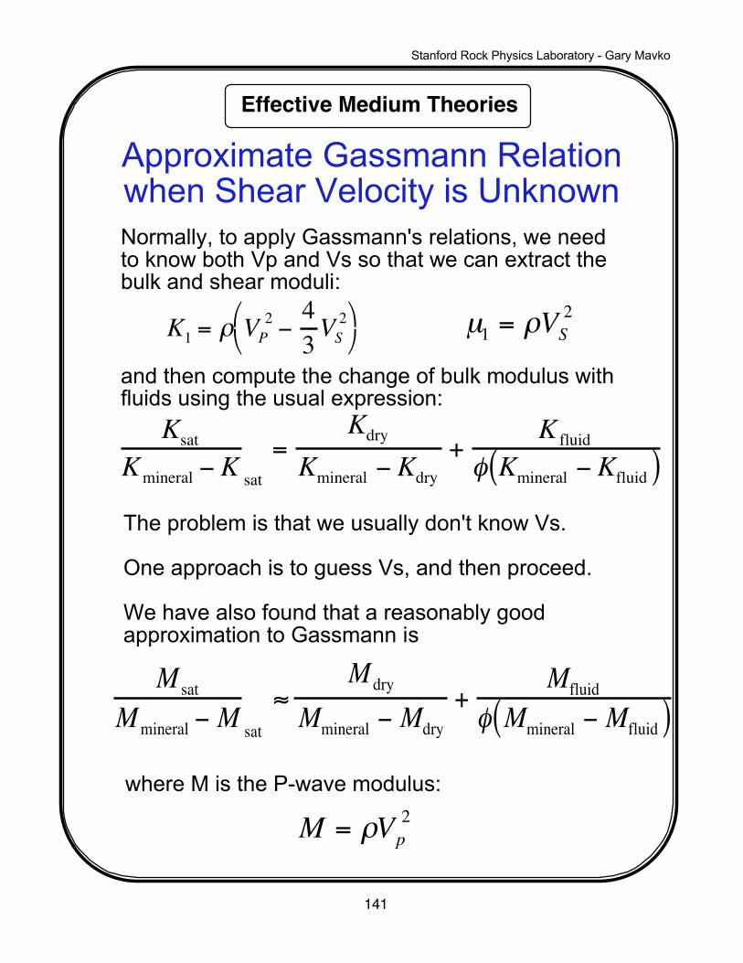
Approximate Gassmann Relationwhen Shear Velocity is UnknownNormally, to apply Gassmann's relations, we needto know both Vp and Vs so that we can extract thebulk and shear moduli:

and then compute the change of bulk modulus withfluids using the usual expression:

The problem is that we usually don't know Vs.

One approach is to guess Vs, and then proceed.

We have also found that a reasonably goodapproximation to Gassmann is

where M is the P-wave modulus:

K1 = ρ VP2 −43VS

2

µ1 = ρVS2

KsatKmineral − K sat

=Kdry

Kmineral − Kdry+

K fluid

φ Kmineral − Kfluid( )

M = ρVp2

M sat

Mmineral − M sat≈

Mdry

Mmineral − Mdry+

Mfluid

φ Mmineral − Mfluid( )



142

Approximate Gassmann RelationWhen Shear Velocity is Unknown

Predictions of saturated rock Vp from dry rock Vp arevirtually the same for the approximate and exactforms of Gassmann’s relations.

Vp-saturated, From GassmannVp-s

atur

ated

, Fro

m A

ppro

ximat

e G

assm

ann



143

Gassmann's is a Low Frequency Relation

It is important to remember that Gassmann’s relationsassume low frequencies. Measured ultrasonic Vp insaturated rocks is almost always faster than saturated Vppredicted from dry rock Vp using Gassmann. Data hereare for shaly sandstones (Han, 1986).



144

Water Flood Example: Pore Pressure Increase and Change From Oil to Brine

Calculated using Gassmann from dry lab data from Troll (Blangy, 1992).Virgin condition taken as low frequency, oil saturated at Peff=30 MPa.Pressure drop to Peff=10 MPa, then fluid substitution to brine.Koil = 1., Kbrine = 2.2

G.12

2 2 . 5

1250

1300

1350

Brine Flood into Oil

Vp (km/s)

dept

h (m

)

Pressure

oil to water

original o i l

oil atincreased Pp

brine atincreased Pp

• effect of pressure on frame• effect of pressure on fluids• frame+fluid: fluid substitution

One typical depth point

(laboratory)



145

Gas Flood Example: Pore Pressure Increase and Change From Oil to Gas

Calculated using Gassmann from dry lab data from Troll (Blangy, 1992).Virgin condition taken as low frequency, oil saturated at Peff=30 MPa.Pressure drop to Peff=10 MPa, then fluid substitution to gas.Koil = 1., Kbrine = 2.2

G.12

1 . 8 2 . 4

1250

1300

1350

Gas Flood into Oil

Vp (km/s)

dep

th (

m)

Pressure

oil to gas

original o i l

oil atincreased Pp

gas atincreased Pp




146

Brine Flood Example: Pore Pressure Decrease and Change From Oil to Brine

Calculated using Gassmann from dry lab data from Troll (Blangy, 1992).Virgin condition taken as low frequency, oil saturated at Peff=25 MPa.Pore pressure drop to Peff=30 MPa, then fluid substitution to brine.Koil = 1., Kbrine = 2.2

1 . 8 2 . 4 3

1250

1300

1350

Brine Flood with Pressure Decline

Vp (km/s)

dept

h (m

)

original o i l

oil atdecreased Pp

brine atdecreased Pp

frame effectdecreased Peff




147

Stiff,deepwater sand, heavy oil (API20,GOR=15, T=75,Pp=18->25,Sw=.3->.8)

Stiff, Turbidite Sand, Heavy OilWater Flood with Pp Increase



148

Deepwater sand, Light oil (API35,GOR=200, T=75Peff=25->18,Pp=18->25, Sw=.3->.8)

Stiff, Turbidite Sand, Light OilWater Flood with Pp Increase



149

Fluid Substitution in Anisotropic Rocks:Brown and Korringa’s Relations

where

effective elastic compliance tensor of dry rock

effective elastic compliance tensor of rock saturated with pore fluid

effective elastic compliance tensor of mineral

compressibility of pore fluid

compressibility of mineral material =

porosity

This is analogous to Gassmann’s relations. To apply it,one must measure enough velocities to extract the fulltensor of elastic constants. Then invert these for thecompliances, and apply the relation as shown.

Sijkl(dry) − Sijkl

(sat ) =Sijαα(dry) − Sijαα

0( ) Sklαα(dry) − Sklαα

0( )Sααββ(dry) − Sααββ

0( ) + βfl − β 0( )φ

Sijkl(dry)

Sijkl(sat )

Sijkl0

β fl

β0

φ

Sααββ0



150

Marion (1990) discovered a simple, semi-empirical way to solve the fluidsubstitution problem. The Hashin-Shtrikman bounds define the range ofvelocities possible for a given volume mix of two phases, either liquid orsolid. The vertical position within the bounds, d/D, is a measure of therelative geometry of the two phases. For a given rock, the bounds can becomputed for any two pore phases, 0 and 1. If we assume that d/Dremains constant with a change of fluids, then a measured velocity withone fluid will determine d/D, which can be used to predict the velocityrelative to the bounds for any other pore phase.

Bounding Average Method (BAM)



151

Velocity in Massilon sandstone saturated with parowax. Data from Wang(1988). Wax saturated velocities were predicted using BAM, from Wang'smeasured velocities in the dry rock and in wax (from Marion, 1990)

2800

3000

3200

3400

3600

3800

4000

4200

0 20 40 60 80 100 120 140

Massillon Light Sandstone

P-V

elo

cit

y (m

/s)

Temperature (°C)

measured parowax

BAMcalculatedparowax

measured dry

G.8

An Example of the Bam Method. The waxsaturated velocities are predicted from the

dry rock velocities.



152

Velocity in dry and saturated Westerly granite. Data from Nur andSimmons (1969). Saturated velocities were predicted using BAM,from measured velocities in the dry rock (from Marion, 1990)

G.9



153

bc

Ellipsoidal Models for Pore Deformation

Most deterministic models for effective moduliassume a specific idealized pore geometry in orderto estimate the pore space compressibility:

The usual one is a 2-dimensional or 3-dimensionalellipsoidal inclusion or pore.

The quantity a = b/c is called the aspect ratio.

1

K φ=

1vpore

∂vpore∂σ

Recall the general expression for the dry rock modulus: 1

K dry= 1

K mineral+ φ

K φ

Gassmann’s relation is a transformation, allowing us to predict how measured velocities areperturbed by changing the pore fluid. Now wediscuss a different approach in which we try to model the moduli “from scratch”.



154

Estimating the Dry Rock Modulus

Mathematicians have worked out in great detail the 3-D deformation field U, of an oblate spheroid (penny-shaped crack) under applied stress. For example, thedisplacement of the crack face is:

We can easily integrate to get the pore volume changeand the dry modulus:

bc

σ

σ

An externally applied compression tends to narrow thecrack, with the faces displacing toward each other.

U(r) = σc

K mineral

4 1 – ν 2

3π 1 – 2ν1 – r

c2

1K dry

= 1K mineral

+ 16 1 – ν 2

9 1 – 2ν1

K mineral

Nc 3

Vbulk



155

"Crack density parameter"

Dry Rock Bulk Modulus

Modulus depends directly on crack density.Crack geometry or stiffness must bespecified to get a dependence on porosity.

1Kdry

=1

Kmineral+16 1− v2( )9 1− 2v( )

1Kmineral

Nc 3

Vbulk

1Kdry

=1

Kmineral1 +

16 1− v2( )9 1− 2v( )

Nc 3

Vbulk

1Kdry

=1

Kmineral1 +

16 1− v2( )9 1− 2v( )

∈

∈=NVbulk

c 3

≈φα

34π



156

Crack Density Parameter

In these and other theories we often encounter thequantity:

This is called the Crack Density Parameter, and has theinterpretation of the number of cracks per unit volume.

Example: 2 cracks per small cell. Each crack about 2/3the length of a cell.

L2c

v = L3

ε =Nc 3

Vbulk

ε =cL

3

≈ 0.07



157

Distribution of Aspect Ratios

Modulus depends on the number of cracks andtheir average lengths

An idealized ellipsoidal crack will close when theamount of deformation equals the original crackwidth:

solving gives:

We generally model rocks as having a distributionof cracks with different aspect ratios. As thepressure is increased, more and more of themclose, causing the rock to become stiffer.

1Kdry

=1

Kmineral+

16 1− v2( )9Kmineral 1− 2v( )

Nc 3

Vbulk

U = b

σclose ≈αKmineral3π41− 2v( )1− v 2( )

≈αKmineral



158

Kuster and Toksöz (1974) fmorulation based on long-wavelength, first order scattering theory (non self-consistent)

KKT* − Km( )

Km +43

µm

KKT* +

43

µm

= xii=1

N

∑ Ki − Km( )Pmi

µKT* − µm( ) µm +ζ m( )

µKT* +ζ m( ) = xi

i=1

N

∑ µ i − µm( )Qmi

ζ =µ69K + 8µ( )K + 2µ( )



159

Self-Consistent EmbeddingApproximation

Walsh's expression for the moduli in terms of the porecompressibility is fairly general. However attempts toestimate the actual pore compressibility are often basedon single, isolated pores.

The self-consistent approach uses a single porein a medium with the effective modulus.

Solving for Kdry gives:

1Kdry

=1

Kmineral+

16 1− v2( )9Kmineral 1− 2v( )

Nc 3

Vbulk

1Kdry

=1

Kmineral+16 1− v 2( )9Kdry 1− 2v( )

Nc3

Vbulk

Kdry = Kmineral 1−16 1− v2( )9 1− 2v( )

Nc3

Vbulk



160

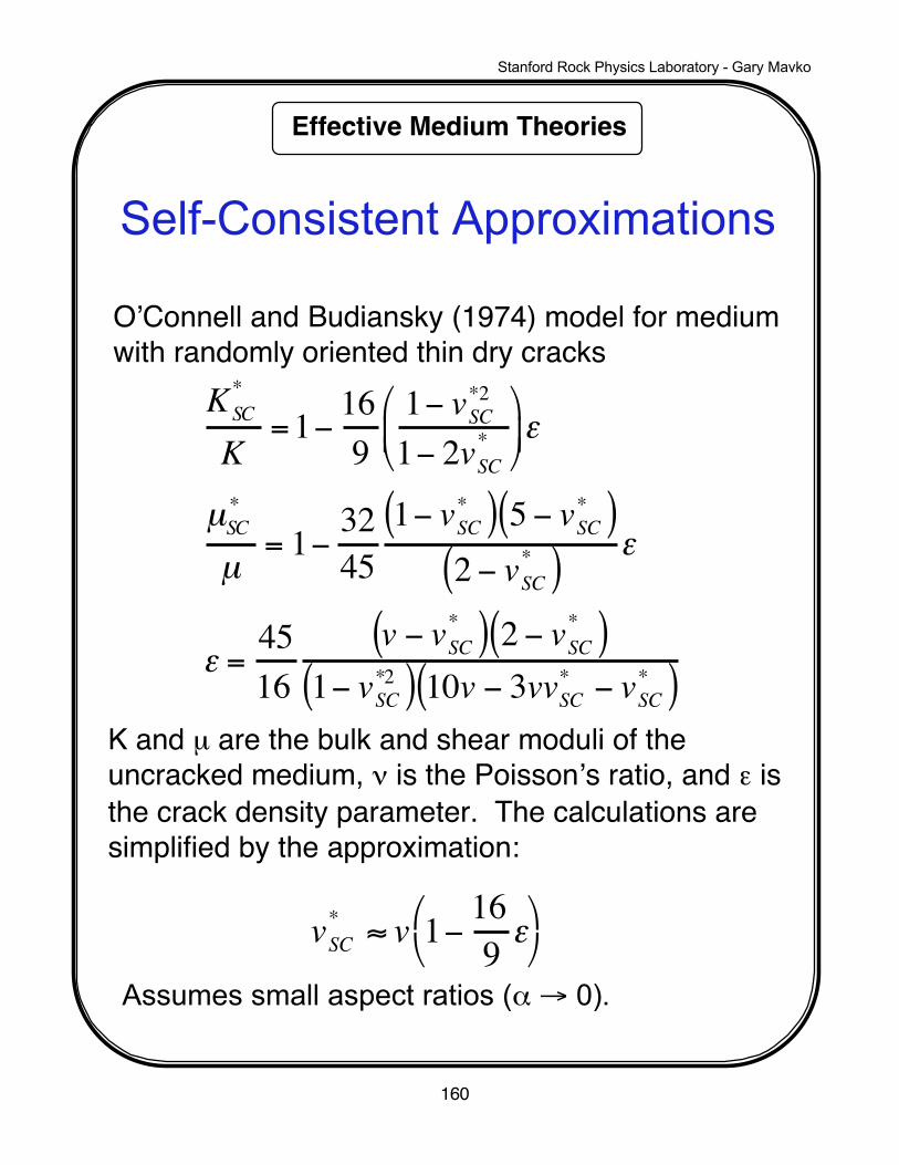
Self-Consistent Approximations

O’Connell and Budiansky (1974) model for mediumwith randomly oriented thin dry cracks

K and µ are the bulk and shear moduli of theuncracked medium, ν is the Poisson’s ratio, and ε isthe crack density parameter. The calculations aresimplified by the approximation:

Assumes small aspect ratios (α → 0).

KSC*

K=1−

169

1− vSC*2

1− 2vSC*

ε

µSC*

µ= 1−

3245

1− vSC*( ) 5 − vSC*( )2 − vSC

*( ) ε

ε =4516

v − vSC*( ) 2 − vSC

*( )1− vSC*2( ) 10v − 3vvSC* − vSC*( )

vSC* ≈ v 1−

169 ε



161

Self-Consistent Approximations

Berryman’s (1980) model for N-phase composites

coupled equations solved by simultaneous iteration

xi Ki − K*( )P*ii=1

N

∑ = 0

xii=1

N

∑ µ i − µ*( )Q*i = 0



162

Comparison of Han's (1986) sandstone data with modelsof idealized pore shapes. At high pressure (40-50 MPa),there seems to be some equivalent pore shape that is

more compliant than any of the convex circular or spherical models.



163

G14

Comparison of self-consistent elliptical crack modelswith carbonate data. The rocks with stiffer pore shapes are fit best by spherical pore models, whilethe rocks with thinner, more crack-like pores are fitbest by lower aspect ratio ellipsoids.

Data from Anselmetti and Eberli., 1997, in Carbonate Seismology, SEG.

Documents

Effective Medium Models - Stanford University Rock Physics Laboratory - Gary Mavko Effective Medium Theories 116 The Voigt and Reuss averages are interpreted as the ratio of average