Embed Size (px)
Citation preview

Effect of vane shape and fertilizer product on spread uniformity using a dual-disc
spinner spreader
by
Ravinder Kaur Thaper
A thesis submitted to the Graduate Faculty of
Auburn University
in partial fulfillment of the
requirements for the Degree of
Master of Science
Auburn, Alabama
August 2, 2014
Keywords: Fertilizer Spreader, Application, Vane, Segregation, Disc, Blended Fertilizer
Copyright 2014 by Ravinder Kaur Thaper
Approved by
John P. Fulton, Chair, Associate Professor of Biosystems Engineering
Timothy P. McDonald, Associate Professor of Biosystems Engineering
Oladiran O. Fasina, Professor of Biosystems Engineering
C. Wesley Wood, Professor and Director, University of Florida West Florida Research
and Education Center

ii
ABSTRACT
Advancements in granular applicators are required in order to provide accurate metering
and placement of fertilizer as emphasis grows on nutrient and associated environmental
stewardship. Spinner-disc spreaders are commonly used to apply granular fertilizers with
current spread widths up to 30 m. Spreader hardware components (divider, spinner disc
and vanes) influence material distribution but increased spread widths have increased the
risk for non-uniform application of nutrients. Therefore, the objectives of this research
were to 1) evaluate the impact of vane design on fertilizer particle behavior and spread
distribution uniformity for a dual-disc spinner spreader, 2) compare and contrast physical
and chemical methods for measuring nutrient concentration of blended fertilizer samples
and 3) determine the segregation potential of a blended fertilizer applied using a dual-disc
spinner spreader while varying feed rate and disc speed. Two types of testing were
conducted; stationary and standard pan testing. A typical fertilizer dual-disc spreader was
used in this study. Treatments included feed rates of 224 and 448 kg ha-1
and three
spinner-disc speeds, 600, 700 and 800 rpm. Four vane designs were also evaluated.
Results indicated that two distinct patterns of the overall spread pattern existed due to
controlled and uncontrolled flow of fertilizer off the vanes. Further, vane design impacted
spread uniformity. The top edge of Vane 2, tapered at 15º backwards, reduced ricocheting
by approximately 50% compared to Vane 1. Vane 2 also produced the most consistent
spread uniformity compared to other three vane designs over the varying disc speeds.

iii
Vane 4, with an enclosed U-section, generated the maximum effective spread width of
24.4 m at a spinner disc speed of 800 rpm versus 22.9 m for Vanes 1, 2 and 3. Overall,
Vane 2 was recommended for fertilizer application using this dual-disc spinner spreader.
The chemical method for analyzing nutrient concentration generated consistently lower
nutrient concentration values for P2O5 and K2O compared to a physical separation
method. The mean difference between the methods was a factor of 1.15. Distinct nutrient
patterns were generated for the different blended fertilizer constituents; “W” shape for
P2O5 and “M” for K2O regardless of feed rate and spinner disc speed. Nutrient spread
distribution patterns did not vary with feed rate (p>.05) whereas the increase in spinner
disc speed caused significant differences (p<.0001) as the pattern widened as speed
increased. DAP particles travelled farther than potash with maximum transverse distance
of 16.4 m at 800 rpm.

iv
ACKNOWLEDGEMENTS
First and foremost, I would like to thank God who gave me strength and courage to
succeed. I would like to express my deepest gratitude to my committee chair Dr. John P.
Fulton who gave me this valuable opportunity. I am in debt to him for his constant
support and expert advice throughout the learning process. Without his guidance and
encouragement, this thesis would not have been possible. I appreciate the feedback from
my committee members Dr. Timothy McDonald, Dr. Oladiran Fasina and Dr. C. Wesley
Wood whose valuable comments have been illuminating. Special thanks go to Greg Pate
and his farm crew who allowed me to conduct my experiments at E.V. Smith Research
Center, Shorter, AL. I would also like to thank everyone in the Biosystems Engineering
Department who helped during my project; especially Dewayne "Doc" Flynn, Christian
Brodbeck and Joy Brown. I would also like to thank Ms. Brenda Wood for her assistance
during laboratory work. I am speechless, and don’t have any words to thank my mother
and late father who always inspired me in my life. My father will be there in my thoughts
forever, he always tried to extract the best of me through all the odds in my life, “love
you so much my sweetest daddy”. My mother has been an inspiration and will always be
in my life. Finally, I would like to thank my husband who has always stood by me
through all the ups and downs. I take this opportunity to thank my friends Simerjeet Virk,
Jonathan Hall, David Herriott, Tyler Phillips, Jarrod Litton, Bruce Faulk, William
Graham, Aurelie Poncet, Oluwatosin Oginni, Oluwafemi Oyedeji and Ryan McGehee.
v
TABLE OF CONTENTS
ABSTRACT ....................................................................................................................................... ii
ACKNOWLEDGEMENTS .............................................................................................................. iv
LIST OF TABLES ..............................................................................................................................x
LIST OF figures .............................................................................................................................. xiv
LIST OF ABBREVIATIONS ........................................................................................................ xvii
Chapter 1 INTRODUCTION ..............................................................................................................1
1.1 Introduction ..............................................................................................................................1
1.2 Justification ..............................................................................................................................4
1.3 Objectives .................................................................................................................................6
1.4 Organization of Thesis .............................................................................................................6
Chapter 2 LITERATURE REVIEW ...................................................................................................8
2.1 Fertilizers for Crop Production ................................................................................................8
2.2 Fertilizers and Properties..........................................................................................................8
2.2.1 Bulk Physical Properties of Granular Fertilizers ............................................................11
2.2.1.1 Bulk Density ...........................................................................................................12
2.2.2 Particle Properties of Granular Fertilizers ......................................................................13
2.2.2.1 Particle Size ............................................................................................................13
2.2.2.2 Particle Density ......................................................................................................17
2.2.2.3 Particle Hardness ....................................................................................................18

vi
2.2.2.4 Coefficient of Friction ............................................................................................18
2.2.3 Chemical Properties of Granular Fertilizers ...................................................................19
2.2.3.1 Nutrient Concentration (N-P2O5-K2O) ...................................................................19
2.2.3.2 Soluble Salts ...........................................................................................................20
2.2.3.3 Solubility ................................................................................................................21
2.3 Types of Granular Fertilizer Applicators ...............................................................................21
2.4 Evaluating Granular Spreader Performance...........................................................................24
2.4.1 Fertilizer Spread Patterns ...............................................................................................25
2.4.1.1 Desirable Spread Patterns ......................................................................................26
2.4.1.2 Undesirable Patterns ...............................................................................................27
2.4.1.3 Simulated Overlap Spread Patterns ........................................................................29
2.5 Standard Methods for Evaluating Granular Applicator Distribution .....................................30
2.6 Fertilizer Physical Properties Impacting Fertilizer Distribution ............................................35
2.6.1 Particle Size ....................................................................................................................36
2.6.2 Particle Shape .................................................................................................................41
2.6.3 Particle Density ..............................................................................................................42
2.6.4 Particle’s Coefficient of Friction ....................................................................................43
2.6.5 Particle Hardness ............................................................................................................44
2.7 Spreader Hardware Parameters Effecting Spread Distribution ..............................................45
2.8 Impact of Non-Uniform Fertilizer Application on Crop Yield ..............................................48
2.9 Discrete Element Modeling (DEM) .......................................................................................49
2.10 Proposed Methods of Reducing Segregation .......................................................................51
2.11 Summary ..............................................................................................................................52

vii
Chapter 3 VANE DESIGN IMPACT ON FERTILIZER DISTRIBUTION FOR A
DUAL-DISC SPINNER SPREADER ..............................................................................................54
3.1 Abstract ..................................................................................................................................54
3.2 Introduction ............................................................................................................................55
3.3 Sub-Objectives .......................................................................................................................57
3.4 Material and Methods ............................................................................................................58
3.4.1 Experimental Design ......................................................................................................61
3.4.2 Stationary Testing ..........................................................................................................61
3.4.3 Standard Pan Testing ......................................................................................................64
3.4.4 Physical Properties .........................................................................................................65
3.4.5 Investigating Particle Behavior ......................................................................................65
3.4.6 Data Analysis .................................................................................................................67
3.5 Results and Discussion ...........................................................................................................68
3.5.1 Physical Properties .........................................................................................................68
3.5.2 Stationary Tests ..............................................................................................................69
3.5.2.1 Vane Design Influence on Overall Particle Exit Point off the Disc .......................69
3.5.2.2 Controlled Material Flow .......................................................................................70
3.5.2.3 Ricocheting .............................................................................................................72
3.5.2.4 Impact of Increase in Spinner Disc Speed on Ricocheting ....................................73
3.5.3 Distribution Pattern Make-Up ........................................................................................75
3.5.4 Standard Pan Tests .........................................................................................................76
3.5.4.1 Standardized Distribution Pattern Analysis ............................................................76
3.5.4.2 Impact of Vane Design on Effective Spread Width ...............................................77

viii
3.5.4.3 Vane Design Impact on Spread Uniformity ...........................................................78
3.5.4.4 Particle Flow Behavior ...........................................................................................80
3.6 Summary ................................................................................................................................81
Chapter 4 COMPARISON OF CHEMICAL VERSUS PHYSICAL METHODS FOR
MEASURING NUTRIENT CONCENTRATION ...........................................................................83
4.1 Abstract ..................................................................................................................................83
4.2 Introduction ............................................................................................................................83
4.3 Methodology ..........................................................................................................................84
4.3.1 Chemical Method ...........................................................................................................84
4.3.2 Physical Method .............................................................................................................86
4.3.3 Inequality Ratio ..............................................................................................................87
4.3.4 Statistical Analysis .........................................................................................................87
4.4 Results ....................................................................................................................................87
4.5 Summary ................................................................................................................................90
Chapter 5 POTENTIAL OF FERTILIZER SEGREGATION DURING APPLICATION
USING SPINNER-DISC SPREADER .............................................................................................91
5.1 Abstract ..................................................................................................................................91
5.2 Introduction ............................................................................................................................92
5.3 Sub-objectives ........................................................................................................................94
5.4 Materials and Methods ...........................................................................................................94
5.4.1 Determination of Physical Properties of Fertilizers .......................................................96
5.4.2 Data Analysis .................................................................................................................96
5.5 Results and Discussions .........................................................................................................97

ix
5.5.1 Fertilizer Physical Properties .........................................................................................97
5.5.2 Single-Pass Nutrient Distribution Patterns .....................................................................97
5.5.3 Simulated Overlap Analysis ...........................................................................................99
5.5.4 Level of Segregation ....................................................................................................103
5.5.5 Spread Distribution Patterns for Potash Application as Single Product and in a
Blend… .................................................................................................................................104
5.6 Summary ..............................................................................................................................105
Chapter 6 CONCLUSIONS ............................................................................................................107
6.1 Summary ..............................................................................................................................107
6.2 Conclusions ..........................................................................................................................110
6.3 Opportunities for Future Research .......................................................................................111
REFERENCES ...............................................................................................................................114
APPENDICES ................................................................................................................................127
APPENDIX A: SPREADER SPECIFICATIONS .........................................................................128
APPENDIX B: TRACTOR SPECIFICATIONS ...........................................................................134
APPENDIX C: RAVEN ENVIZIO PRO SPECIFICATIONS ......................................................135
APPENDIX D: MASS OF POTASH COLLECTED BY ZONE FOR THE
STATIONARY TESTS IN CHAPTER 3 .......................................................................................136
APPENDIX E: SUMMARIZED DATA TABLES AND FIGURES ALONG WITH
INCLUDED STATISTICS. ............................................................................................................140
APPENDIX F: SAS PROGRAM CODE FOR ZONE ANALYSIS IN CHAPTER 3 ...................149
APPENDIX G: STATISTICAL RESULTS ...................................................................................156

x
LIST OF TABLES
Table 2.1. Common individual fertilizer sources and their nominal concentration levels
(Fert. Technologies, 2011). .......................................................................................................10
Table 2.2. Reported bulk densities for both individual fertilizer constituents and typical
blends. .......................................................................................................................................13
Table 2.3. Variation in median particle size of for different fertilizers and common
blends. .......................................................................................................................................15
Table 2.4. Variation in particle size distribution of different fertilizer sources including a
blend. .........................................................................................................................................17
Table 2.5. Variation in particle density and hardness for different base granular fertilizers. ........18
Table 2.6. Variation in coefficient of friction for different fertilizers (Hofstee and
Huisman, 1990). ........................................................................................................................19
Table 2.7. Salt indices of various fertilizers (Oldham, 2008). .......................................................21
Table 3.1. Description of Zones 1 through 7. ................................................................................64
Table 3.2. Average physical properties for Potash (KCl) used during this study. Standard
deviation presented in parenthesis. ...........................................................................................69
Table 3.3. Overall average of percent material mass (%) measured by zone for each vane
design by spinner disc speed at feed rate of 224 kg ha-1
. ..........................................................70
Table 3.4. Average percent material captured by zone when considering only Zones 2
through 6 or zones where controlled distribution occurred at feed rate of 224 kg ha-1
. ...........72
Table 3.5. Average percent material captured by zone when considering only Zones 2
through 6 or zones where controlled distribution occurred at feed rate of 224 kg ha-1
. ...........72
Table 3.6. Impact of increase in spinner disc speed on effective spread width for the
Vanes 1, 2, 3 and 4. ...................................................................................................................78
Table 4.1. Results of nutrient concentration conducted by two different people (labeled
A and B) in the lab on the same sample using the chemical method. .......................................88
Table 4.2. Nutrient concentration results for running three samples twice using the
chemical method. ......................................................................................................................88

xi
Table 4.3. Mean P2O5 and K2O concentrations determined using the chemical and
physical methods with standard deviation presented in parenthesis. The difference
between the two methods is also presented in the last two columns. .......................................89
Table 5.1. Measured physical properties for the 10-26-26 blend along with individual
constituents consisting of Di-ammonium Phosphate (DAP) and Potash (KCl).
Standard deviation presented in parenthesis. ............................................................................97
Table 5.2. Effective spread widths determined for DAP and Potash over the different
spinner disc speeds. .................................................................................................................100
Table 5.3. Mass proportions (%) between DAP and Potash within each collection pan
across the swath width for each of the spinner disc speed treatments. ...................................102
Table 5.4. Representation of the influence of various parameters on the level of
segregation. .............................................................................................................................104
Table D.1. Mass of potash collected in different zones of collection device for Vane 1. ...........136
Table D.2. Mass of potash collected in different zones of collection device for Vane 2. ...........137
Table D.3. Mass of potash collected in different zones of collection device for Vane 3. ...........138
Table D.4. Mass of potash collected in different zones of collection device for Vane 4. ...........139
Table E.1. Overall mean mass material distribution (%) for all four vane shapes at feed
rate of 448 kg ha-1
in different zones of the collection device at three spinner disc-
speeds of 600, 700 and 800 rpm..............................................................................................140
Table E.2. Overall mean mass material distribution (%) within in Zones 2 and 6 at feed
rate of 224 kg ha-1
, along with p-values comparing data within a specific treatment............140
Table E.3. Overall mean mass material distribution (%) within Zones 3 and 5 at feed rate
of 448 kg ha-1
along with p-values comparing data within a specific treatment. ....................141
Table E.4. Average percent material captured by zones when considering only Zones 2
through 6 or zones where controlled distribution occurred at feed rate of 224 kg ha-1
. .........141
Table E.5. Average percent material captured by zone when considering only Zones 2
through 6 or zones where controlled distribution occurred at feed rate of 224 kg ha-1
. .........143
Table E.6. Impact of increase in spinner disc speed on maximum transverse distance by
Vane. .......................................................................................................................................143
Table E.7. Summary of the overlap pattern analyses at effective spread widths of 18.3
and 21.3 m for the four vane designs along with skewing. .....................................................144
Table E.8. Impact of increase in spinner disc speed on the level of segregation for P2O5
and K2O at all transverse pan locations across the swath. ......................................................147
Table E.9. The impact of increase in feed rate on level of segregation represented by p-
values on nutrient concentration distribution for P2O5 and K2O at all transverse pan
locations across the swath. ......................................................................................................148

xii
Table G.1. ANOVA results comparing mass collection in different zones of collection
device at feed rates of 224 kg ha-1
and 600 rpm disc-speed for Vanes 1, 2, 3 and 4. .............156
Table G.2. ANOVA results comparing mass collection in different zones at feed rate of
224 kg ha-1
and 700 rpm disc-speed for Vanes 1, 2, 3 and 4. .................................................157
Table G.3. ANOVA results comparing mass collection in different zones at feed rate of
224 kg ha-1
and 800 rpm disc-speed for Vanes 1, 2, 3 and 4. .................................................158
Table G.4. ANOVA results comparing mass collection in different zones at feed rate of
448 kg ha-1
and 600 rpm disc-speed for Vanes 1, 2, 3 and 4. .................................................159
Table G.5. ANOVA results comparing mass collection in different zones at feed rate of
448 kg ha-1
and 700 rpm disc-speed for Vanes 1, 2, 3 and 4. .................................................160
Table G.6. ANOVA results comparing mass collection in different zones in Vane 2 at
feed rates of 224 kg ha-1
and 448 kg ha-1
. ...............................................................................162
Table G.7. ANOVA results comparing mass collection in different zones of collection
device at feed rates of 224 kg ha-1
and 448 kg ha-1
in Vane 1. ...............................................163
Table G.8. ANOVA results comparing mass collection in different zones of collection
device at three different spinner disc speeds of 600, 700 and 800 rpm in Vane 1 at feed
rate of 224 kg ha-1
. ..................................................................................................................164
Table G.9. ANOVA results comparing mass collection in different zones of collection
device at three different spinner disc speeds of 600, 700 and 800 rpm in Vane 1 at feed
rate of 448 kg ha-1
. ..................................................................................................................166
Table G.10. ANOVA results comparing mass collection in different zones of collection
device at three different spinner disc speeds of 600, 700 and 800 rpm in Vane 2 at feed
rate of 224 kg ha-1
. ..................................................................................................................167
Table G.11. ANOVA results comparing mass collection in different zones of collection
device at three different spinner disc speeds of 600, 700 and 800 rpm in Vane 2 at feed
rate of 448 kg ha-1
. ..................................................................................................................168
Table G.12. ANOVA results comparing mass collection in different zones of collection
device at feed rates of 224 kg ha-1
and 448 kg ha-1
in Vane 3. ...............................................170
Table G.13. ANOVA results comparing mass collection in different zones of collection
device at three different spinner disc speeds of 600, 700 and 800 rpm in Vane 3 at feed
rate of 224 kg ha-1
. ..................................................................................................................171
Table G.14. ANOVA results comparing mass collection in different zones of collection
device at three different spinner disc speeds of 600, 700 and 800 rpm in Vane 3 at feed
rate of 448 kg ha-1
. ..................................................................................................................173
Table G.15. ANOVA results comparing mass collection in different zones of collection
device at feed rates of 224 kg ha-1
and 448 kg ha-1
in Vane 4. ...............................................174
Table G.16. ANOVA results comparing mass collection in different zones of collection
device at three different spinner disc speeds of 600, 700 and 800 rpm in Vane 4 at feed
rate of 224 kg ha-1
. ..................................................................................................................175

xiii
Table G.17. ANOVA results comparing mass collection in different zones of collection
device at three different spinner disc speeds of 600, 700 and 800 rpm in Vane 4 at feed
rate of 448 kg ha-1
. ..................................................................................................................177

xiv
LIST OF FIGURES
Figure 1.1. Comparison of world population and corresponding food demand from 1970
through projections for 2050 (FAO, 2012). ................................................................................1
Figure 1.2. U.S. fertilizer prices since 1960 (ERS-USDA, 2012). ..................................................3
Figure 2.1. Rear view of a dual-disc spinner spreader illustrating the various hardware
components used for conveying and distributing fertilizer and lime. .......................................22
Figure 2.2. An example of a pneumatic fertilizer applicator during field operation. The
aluminium pipes are used to convey fertilizers to deflectors along the boom for
material distribution. .................................................................................................................23
Figure 2.3. Desirable single-pass distribution patterns typical for dual-disc spinner
spreaders; flat top (a), oval or Gaussian (b) and pyramid-shaped (c) (ACES, 2010). ..............27
Figure 2.4. “M” shaped single-pass distribution pattern (ACES, 2010). .......................................28
Figure 2.5. “W” shaped single-pass distribution pattern (ACES, 2010). ......................................28
Figure 2.6. Skewed single-pass distribution pattern (ACES, 2010). .............................................28
Figure 2.7. Typical field path taken by a spreader operator where back and forth passes
are made. This type of path is referred to as the progressive application method. ..................30
Figure 2.8. Graphical representation of using a single-pass pattern to generate the
simulated overlap spread pattern indicated by the orange dots and line. ..................................30
Figure 2.9. Graphical representation using a single pass pattern to generate the simulated
overlap spread pattern (ASABE Standards, 2009). Effective spread width and
resulting application rate line are labelled. ...............................................................................32
Figure 2.10. Example illustrating the typical CV (%) versus spread width curve. The
point where the curve crosses the CV=15% at the maximum spread width establishes
the effective spread width for a specific spreader and product. ................................................33
Figure 2.11. Illustration of how effective spread would change as spinner disc speed
increases. ...................................................................................................................................33
Figure 3.1. Rear view image of the spreader showing arrangement of vanes on spinner
discs and different hardware components. ................................................................................59

xv
Figure 3.2. Front and Isometric views along with geometric dimensions for the four
different vane designs. Additional views provided to highlight differences between
vane designs. .............................................................................................................................61
Figure 3.3. Top view of spinner discs and collection device (showing zones 2 through 6)
used to evaluate exit location of fertilizer particles from discs and vanes. The figure
also illustrates zone divisions and their location relative to the disc and back plate.
Zone 1 (shaded region) collected material below and between the spinner discs. ...................63
Figure 3.4. Illustration of the fabricated collection device mounted on the spreader and
containers used to accrue material by zone. ..............................................................................63
Figure 3.5. Example of CV (%) versus effective spread width (m) at the three spinner-
disc speeds of 600, 700 and 800 rpm of the fertilizer spreader. The three points
indicated the minimum CVs and thereby effective spread width at the respective
spinner disc speed. ....................................................................................................................68
Figure 3.6. Representation of ricocheting % (i.e. uncontrolled material flow) ± 1 SD for
all the four vane shapes, a. 224 kg ha-1
b. 448 kg ha-1
. Means denoted by the same
letters are not significantly different (α = 95%). .......................................................................73
Figure 3.7. Depiction of the two spread patterns which make up the overall single-pass
spread pattern based on EDEM simulations. One pattern represents the controlled
material distribution and the other uncontrolled. ......................................................................76
Figure 3.8. Mean average standardized distribution patterns for all vanes; designated as 1,
2, 3 and 4 at feed rate of 224 kg ha-1
over spinner disc speeds of a) 600 rpm, b) 700
rpm and c) 800 rpm. Each curve in the graph represents mean of three replications.
Transverse location represents the position of pans on the spread width, 0 represents
the point of travel of the spreader with negative points on the left hand side of the
spreader and positive points on right hand side of the spreader. ..............................................77
Figure 3.9. Plot of spread uniformity (CV; %) versus effective spread width for Vane 1
(left) and Vane 2 (right) over different disc speeds. .................................................................79
Figure 3.10. Plot of spread uniformity (CV; %) versus effective spread width for Vane 3
(left) and Vane 4 (right) over different disc speeds. .................................................................79
Figure 3.11. Illustration of material flow and ricocheting off Vane 1. ..........................................81
Figure 3.12. Material flow off Vane 3 (left) versus Vane 4 (right). Note the absence of
ricocheting for Vane 4. ..............................................................................................................81
Figure 4.1. Comparisons between original chemical, final chemical and physical data for
P2O5 and K2O at two feed rates 224 kg ha-1
(a and b) and 448 kg ha
-1 (c and d). .....................90
Figure 5.1. Nutrient concentration patterns for P2O5 (left) and K2O (right) at a feed rate of
224 kg ha-1
. Transverse location represents pan positions at different locations across
the swath. ..................................................................................................................................98
Figure 5.2. Illustration for influence of increase in feed rate on nutrient concentration
distribution patterns for percentages of P2O5 (left) and K2O (right). Transverse
location represents pan positions at different locations across the swath. ................................99
xvi
Figure 5.3. Simulated overlap patterns for percentages of P2O5 and K2O. Transverse
location represents pan positions at different locations across the swath. ..............................100
Figure 5.3. Graphical representation of standardized distribution patterns representing
potash applied as a blend (10-26-26) versus a single product at feed rate of 224
kg ha-1
over spinner disc speed of 800 rpm.............................................................................105
Figure A.1.Rear view of the agricultural fertilizer and lime spreader used in this research. ......128
Figure A.2. Hydraulic circuit for the conveyor and spinner discs (Chandler Spreaders,
2013). ......................................................................................................................................129
Figure A.3. Exploded view of spinner assembly (Chandler Spreaders, 2013). ...........................130
Figure A.4. Exploded view of flow divider assembly (Chandler Spreaders, 2013). ...................131
Figure A.5. Conveyor Assembly (Chandler Spreaders, 2013). ...................................................132
Figure A.6. Electronically adjustable proportional pressure compensated flow controls
(EFC). EFC12-10-12 (Left) and EFC12-15-12R22(Right) ....................................................133
Figure B.1. John Deere 7230 Tractor. ..........................................................................................134
Figure C.1. RAVEN ENVIZIO PRO and switch pro displaying calibration settings for the
spreader ...................................................................................................................................135
Figure E1. Impact of increase in spinner-disc speed on ricocheting (± 1 SD) for all the
four vane shapes at a feed rate of 224 kg ha-1
. Means denoted by the same letters are
not significantly different (α = 95%). .....................................................................................145
Figure E2. Standardized distribution patterns at 224 kg/h and 448 kg/ha for each vane
design. Each curve within the plot represents the mean of three replications.
Transverse location represents pan position across the spread width; 0 represents the
centreline of the spreader with negative values the left side of the spreader and
positive values on the right. ....................................................................................................146

xvii
LIST OF ABBREVIATIONS
CV coefficient of variation
DAP diammonium phosphate
kg m-3
kilograms per cubic meter
kg ha-1
kilograms per hectare
K2O potassium oxide
m meter
mm millimeter
m s-1
meter per second
P2O5 phosphorous oxide
rpm number of rotations per minute

1
Chapter 1 INTRODUCTION
1.1 Introduction
The world population continues to increase and is predicted to reach 9.15 billion by
the year 2050 (FAO, 2012). Concurrently, the middle class is growing in number
worldwide and expanding their diet to include meat (Delgado, 2003) increasing the
demand of feed and thereby grain crops to support animal production. The economies
and social classes are also growing in developing countries placing additional demand on
food production to support the world population. With the increase in world population
and preferred diets, it is projected there needs to be an increase of 60% to 110% in food
production by the year 2050 (Science Daily, 2013) in order to match worldwide demand
(fig. 1.1).
Figure 1.1. Comparison of world population and corresponding food demand from 1970 through projections for
2050 (FAO, 2012).
The three primary options for increasing the world’s food production are: 1)
increase the amount of cultivated lands, 2) increase crop yields on existing lands being
0
1000
2000
3000
4000
2
4
6
8
10
1970 1990 2010 2030 2050
Per
Ca
pit
a F
oo
d C
on
su
mp
tio
n
(kca
l/p
ers
on
/day)
Wo
rld
Po
pu
lati
on
(B
illio
ns)
Year
World Population
Food Consumption
2
used for production, or 3) a combination of both. At the global scale, crop production has
been found to increase by 30% to 50% as a result of fertilization (Stewart et al., 2005). It
has been reported that sustained yield growth is impossible without the use of fertilizer
(Larson and Frisvold, 1996). Fertilizers are required for optimum crop growth providing
crops the necessary nutrients. They replace soil nutrients consumed by prior crops and are
responsible for 40% to 60% of world’s food supply (Borlaug, 2008). Thus, worldwide
fertilizer use continues to increase and expected to reach 199 million tons by 2030
(Liederke, 2008). The U.S. ranks second with 14.9% of the world’s total fertilizer
consumption with an annual usage of 21 million tons (USDA, 2010).
Fertilizer prices have also increased over time (fig. 1.2) with limited expansion of
agricultural lands in the future. The judicious use of fertilizers to minimize application in
environmentally sensitive areas and avoid over-application is required today at the farm
level. Excess usage of fertilizers can result in surface run-off or leaching into ground and
subsurface water bodies causing environmental risks. Hence, the agriculture sector must
improve fertilizer usage including the placement and metering accuracy in order to
minimize off-target or uneven distribution. From an application perspective, spread
uniformity and application accuracy is required on modern application equipment to
ensure sound nutrient stewardship for crop and pasturelands.

3
Figure 1.2. U.S. fertilizer prices since 1960 (ERS-USDA, 2012).
In the U.S., dual-disc spinner spreaders are commonly used to apply granular
fertilizers and lime since they have large spread widths and inexpensive (Oleislagers et
al., 1996) compared to other application equipment. For these types of large spreaders
used on farms, fertilizer is dropped onto two rotating spinner discs from a conveyor chain
or belt with particles accelerated by vanes mounted on the discs for distribution onto the
ground. Spinner disc speed is the primary control of spread width, with 600 to 800 rpm
being common to generate widths between 18.3 and 30.5 m. Hofstee and Huisman
(1990) determined that a correlation existed between spread uniformity and fertilizer
quality. Main factors that affect spread uniformity can be categorized into spreader
hardware design and fertilizer physical properties. Spinner disc spreaders can be sensitive
to variations in material flow rate, physical characteristics of fertilizers such as size,
shape and friction coefficient, wind disturbances, field terrain and vibrations (Moshou et
al., 2004). Tissot et al. (2002) indicated that modern agriculture requires applicators
perform well in order to optimize fertilizer use. Uneven application can lead to reduced
0
200
400
600
800
1000
1960 1980 2000 2020
Pri
ce
($/1
00
0 k
g)
Year
Urea
Ammonium Nitrate
Potassium Chloride

4
crop yield and reduction in agronomic efficiency of fertilizers. Non-uniform distribution
causes the greatest financial losses (Richards, 1985), whereas errors in application rates
affect crop yield and over-application increasing the risk of environmental impacts.
1.2 Justification
Food, fiber, feed and fuel production plus preserving our natural resource base such
as having clean water are important for the global population. Crop production must
increase in order to provide the necessary food for future generations but production
should be conducted in a sustainable manner. Today, off-site transport of nitrogen (N)
and phosphorous (P) must be minimized or eliminated from agricultural lands. However,
fertilizer supplying the proper crop nutrition is required for maximizing crop yields and
farm profitability while sustaining the production of food, fiber, feed and fuel worldwide.
Therefore, applying fertilizer must be conducted in a manner with environmental
stewardship at the forefront. Further, input stewardship includes efficient nutrient
utilization for effective nutrient uptake by crops and pastures.
Over-application of fertilizers can potentially impact the environment by polluting
waterways and underground water supplies due to surface run-off or leaching,
respectively. To help promote and improve fertilizer stewardship, the fertilizer industry
developed the 4Rs to nutrient stewardship program. The 4Rs to nutrient stewardship
emphasizes maintaining the right source, right rate, right time and right place of
fertilizers (Garcia, 2012). Today’s goal related to nutrient management is to increase crop
production while enhancing environmental stewardship. Fertilizer spread uniformity and
accuracy is a key focus during application. Fertilizers are expensive so they must be used
judiciously. Precision agriculture (PA) technologies such as rate controllers permit

5
accurate metering of fertilizers whereas guidance technology reduces overlap and thereby
over-application of inputs. Automatic guidance allows spreaders to traverse the same
field path during subsequent applications, thus coupling the risk of uneven soil fertility
levels if non-uniform distribution of fertilizer occurs. All of these points together can
generate varying soil fertility levels which cannot be afforded by today’s farmers.
Dual-disc spinner spreaders remain a common fertilizer applicator in the U.S. In
terms of area covered per year, spinner spreaders significantly cover more acres for
applying fertilizer and lime than other types of applicators. The spreader parameters
which influence performance including material distribution are vane, spinner disc and
flow divider design along with conveyor design and gate height. It is important that they
are designed to maintain accurate metering and placement of fertilizers. Vane shape is
considered a significant component of spinner spreaders as it controls the effective spread
width along with material distribution by impacting particle flow behavior on the spinner
discs and exit point off the vane/disc assembly. From a design perspective, “controlled”
material flow by the spreader hardware provides the ability to uniformly apply fertilizer
whereas “uncontrolled” behavior generates a state where the spreader hardware is unable
to distribute fertilizer properly. In other words, controlled fertilizer conveyance and
distribution on a spinner spreader is desired and allows for calibration to deliver product
accurately and uniformly. Limited research exists documenting the effect of vane design
on particle flow behavior and spread uniformity for dual disc-spinner spreaders.
In summary, poor and inaccurate application of fertilizers can increase
environmental and farm profitability risks. One issue is that poor spread uniformity could
lead to streaking of soil fertility levels potentially impacting crop yields. Segregation

6
could occur when applying blended fertilizers using modern spinner spreaders especially
considering the large spread widths (e.g. 27.4 to 34.5 m) being used today. Therefore, this
research investigates the ability to enhance spread uniformity of dual-disc spinner
spreaders in order to minimize issues during application of granular fertilizers and meet
performance expectations by farmers implementing new strategies such as site-specific
management (SSM) of nutrients.
1.3 Objectives
The goal of this research focused on enhancing the spread uniformity of dual-disc,
fertilizer spreaders to improve placement of nutrients. The overall research objectives
were to:
1) Evaluate the impact of vane design on fertilizer particle behavior and
spread distribution uniformity for a dual-disc spinner spreader.
2) Compare and contrast physical and chemical methods for measuring
nutrient concentration across the swath width when applying a blended
fertilizer.
3) Determine the segregation potential of a blended fertilizer applied using a
dual-disc spinner spreader while varying feed rate and disc speed.
1.4 Organization of Thesis
Chapter 1 provides an introduction to this research along with justification and
overall objectives. Chapter 2 presents a review of literature detailing information on
fertilizers and various factors impacting application using dual-disc spreaders. Chapter 3
is written in manuscript format and covers the effect of vane design on fertilizer particle

7
flow behavior and spread distribution for a dual-disc spinner spreader. Chapter 4 outlines
the differences between chemical analysis and manual physical methods for determining
nutrient concentration across the swath width for a blended product. Potential of
segregation in a blended fertilizer application while using dual-disc spinner spreaders
with variation in feed rate and disc speeds is covered in Chapter 5. Finally, Chapter 6
summarizes this research highlighting overall conclusions and future research
suggestions.

8
Chapter 2 LITERATURE REVIEW
2.1 Fertilizers for Crop Production
Soil nutrients are essential for crop production and represent a vital component for
sustainable agriculture. Fertilizer provides a source of nutrients and is required for
optimal crop growth. Soils contain natural reserves of nutrients but a majority of them
can remain unavailable to plants during the growing season. As plants grow, they extract
nutrients from the soil and if not replenished, crop growth and yield will be negatively
impacted. Fertilizers are supplied prior or during the growing season. In the US, spinner
disc spreaders are commonly used to apply granular forms of fertilizers but can pose
concerns relative to accurate placement and uniform distribution across cropped fields
and pastures. The following information provides details on fertilizer types along with
their physical and chemical properties with an overview of spinner-disc spreaders and
those factors which impact spread quality.
2.2 Fertilizers and Properties
Commonly used granular fertilizers in agriculture contain three basic macro-
nutrients; nitrogen (N), phosphorous (P) and potassium (K). Nitrogen is a structural
component of proteins, DNA and enzymes which are required for healthy growth of
plants. Phosphorous is also a structural component of DNA and helps in energy storage,
conversion, stem development and a strong root network. Potassium aids in stem

9
development and strong root network as well as promotes flower production which
increases crop yield (Shakhashiri, 2014).
Fertilizer sources can be classified into two categories 1) inorganic and 2) organic.
Organic fertilizers are derived from natural sources like plant and animal wastes. In the
U.S., most organic fertilizers used in crop production are animal manures, swine, beef,
dairy and poultry (Weekend Gardener, Monthly Web Magazine, 2014). These fertilizers
normally require microbial activity in order for nutrients to become plant available.
Organic fertilizers enhance biological activity in the soil and improve soil health over
long term. However, insufficient amounts of organic fertilizers exist in the US to supply
the needed crop nutrients on an annual basis. Therefore inorganic fertilizers are required
and make up the primary source of nutrients in US farming.
Inorganic fertilizers are manufactured, synthetic sources of nutrients. Mined
deposits of phosphate rock and potash are processed in fertilizer manufacturing plants to
produce the required grades of nutrients containing nitrogen, phosphorous or potassium
in fertilizers ready to field apply. In some cases as with potash, it is mined and simply
processed through crushing to the appropriate particle size. Inorganic fertilizers are
soluble with nutrients immediately available to growing plants. They generally are
required in small amounts as they contain high nutrient concentrations (Chen, 2006).
Inorganic fertilizers supply deficient nutrients in the soil rapidly for crops. They can also
be formulated to specific crop needs. Applied fertilizer helps increase yields and
biological activity in the soil (Haynes and Naidu, 1998). Inorganic fertilizers are
generally applied as a single product (Table 2.1), in a blended form or as a liquid solution
(Hart, 1998).

10
Table 2.1. Common individual fertilizer sources and their nominal concentration levels (Fert.
Technologies, 2011).
Material Nutrient Concentration
N- P2O5-K2O-S (%)
Ammonium nitrate 34-0-0-0
Ammonium sulfate 21-0-0-24
Urea 46-0-0-0
Diammonium phosphate (DAP) 18-46-0-0
Triple Super Phosphate (TSP) 0-46-0-0
Muriate of potash (KCl) 0-0-60-0
Based on the nutrient concentration (N-P2O5-K2O), fertilizers are commonly
referred to as single product fertilizers or multiple nutrients. As an example, muriate of
potash (0-0-60) contains only one macronutrient; potassium thereby called a single
product. Therefore, potash contains 60% K2O. DAP (18-46-0) on the other hand includes
both nitrogen and phosphorous therefore termed a multi-nutrient fertilizer. As an example
ammonium sulfate is 21% nitrogen and 23% sulfur.
Blended fertilizers are used since they supply more than one nutrient source.
Common examples of blended fertilizers are 13-13-13, 20-20-20, and 10-26-26 which are
produced using a combination of single products as those listed in Table 2.1. The term
blended is used to describe the formulation process where major fertilizer components
nitrogen (N), phosphorous (P) and potassium (K) occur in separate particles, but are
mechanically mixed or blended without chemical reaction to form a desired nutrient ratio.
Blends can be specifically manufactured or mixed in accordance to specific soil and crop
needs. Blended fertilizers have several advantages compared to single product fertilizers.
A range of different products can be produced by using only basic materials (Formisani,
2005). Application of fertilizers in blended form is economical as it helps in reducing the
number of passes across fields in comparison to single product fertilizer application (Yule

11
and Pemberton, 2009). The process of blending offers flexibility in providing a range of
nutrient concentrations (Miserque and Pirard, 2004). Bulk blending provides a practical
and cost effective way to produce maximum crop yields. As a result, bulk blends
constitute around 70% of the total granular fertilizers sold in the US (Formisani, 2005).
Fertilizers may also contain other nutrients, called micro-nutrients, such as sulfur
(S), iron (Fe), boron (B), zinc (Zn) and molybdenum (Mo). Micronutrients are essential
for crops but are taken up by plants in small quantities. As an example zinc is required for
protein synthesis in plants for seed production and maturity. Likewise, iron aids in
chlorophyll formation in plants. These micro-nutrients are added as additional nutrients
or may be constituents (impurities) remaining in the fertilizer material following mining
and manufacturing processes.
Liquid fertilizers also exist as nutrient sources for crops. Generally, these fertilizers
are applied using sprayers or side-dress units. These fertilizers are quickly absorbed by
plants and boost plant growth. Nutrients are either soil absorbed for plant root uptake or
absorbed foliarly. Urea Ammonia Nitrate (UAN) is commonly used liquid fertilizer. For
the research at hand, granular fertilizers and the application of them are the focus.
Therefore, liquid fertilizers and their properties will not be discussed.
2.2.1 Bulk Physical Properties of Granular Fertilizers
The physical properties of granular fertilizers vary between different products but
also within a single product. This variation occurs depending on the origin of the product,
type of manufacturing process the fertilizer underwent, handling (Hoffmesiter et al.,
1964), storage and transportation. Physical properties and their variation influence
conveyance, storage, transportation and application of fertilizers.

12
2.2.1.1 Bulk Density
It refers to the mass ratio of a sample to the volume it occupies with a unit of kg
m-3
for granular fertilizers. The total volume includes particle volume, inter-
particle void volume, and internal pore volume. Generally, bulk density is
reported in two possible ways; 1) loose bulk density or 2) tap bulk density.
Loose bulk density is defined as the density obtained by pouring a fertilizer
sample into a vessel of known volume without any consolidation. Tap bulk
density is similar but the vessel is tapped or packed. This tapping procedure is
accomplished by repeatedly dropping the vessel from a specified height at a
constant drop rate until the apparent volume of the sample becomes nearly
constant.
Bulk density can vary within and between different fertilizer products
(Table 2.2). Ammonium nitrate (34-0-0) has a bulk density of 800-900 kg m-3
and ammonium sulfate (21-0-0) 700-800 kg m-3
(Solutions for Agriculture,
2013). Both the products provide nitrogen (N) but their bulk density values
differ. Sources of phosphorous such as DAP (18-46-0) and the blend, 10-34-0
supply nitrogen but have different bulk densities; 900-1000 kg m-3
and 1400 kg
m-3
(Solutions for Agriculture, 2013).

13
Table 2.2. Reported bulk densities for both individual fertilizer constituents and typical blends.
Product
Nutrient Concentration
N-P2O5-K2O (%)
Bulk Density
(kg m-3
)
Ammonium nitrate 34-0-0 800-9001
Ammonium sulfate 21-0-0 700-8001
Urea 46-0-0 700-8001
Diammonium phosphate (DAP) 18-46-0 900-1000
1
1040 (tapped)2
Muriate of Potash (KCl) 0-0-60 900-10001
Triple Super Phosphate (TSP) 0-46-0 1000-12001
Blend 28-0-0 13001
Blend 32-0-0 13001
Blend 10-34-0 14001
Blend 20-20-20 7003
Blend 13-13-21 9004
Blend 15-15-15 9004
1) Solutions for Agriculture, 2013
2) The Mosiac Company, 2013
3) Material Safety Data Sheet, 2010
4) Tissot et al., 1999
2.2.2 Particle Properties of Granular Fertilizers
Particle properties of fertilizers vary among and between different sources of
fertilizers. Mean particle size, Size Guide Number (SGN), particle density,
particle hardness constitute the main physical properties of fertilizer particles.
These are important to understand as they can reflect the quality of a fertilizer
and ability of an applicator to spread the material. The follow defines and
discusses each of these particle physical properties in more detail.
2.2.2.1 Particle Size
Particle size represents an important physical property which serves as an
indicator of both quality of a fertilizer product but also the size uniformity or
variability of size for a material. This variable represents the size dimension of
a particle typically reported as a mean or median diameter when discussing
14
granular fertilizers. Particles are three dimensional objects so there are different
measures to express their size are discussed.
i) Median Particle Size (d50) and Size Guide Number
(SGN): Median particle size (d50) represents the median diameter of
fertilizer particles in a sample and is reported using the term d50. As an
example, a d50 = 1.0 mm indicates that 50% of the particles have a
diameter greater than 1.0 mm with the other 50% less than this value.
Mean particle size will typically vary between and among fertilizer
products. Table 2.3 provides d50 for various fertilizers. Urea can have a
d50 of 2.2 mm (Aphale et al., 2003) whereas ammonium sulfate is
usually smaller in size having a d50 around 1.5 mm (Hofstee and
Huisman, 1990). Both of these products are base sources for N but have
significantly different median particle sizes. Potassium particles are
considered to be greater in size compared to nitrogen. As an example,
potassium chloride (KCl) was reported to have a d50 equal to 2.3 mm
(Aphale et al., 2003). When looking at phosphorous sources, they are
typically larger than nitrogen and potassium. Triple super phosphate can
have a d50 around 2.7 mm (Yildirim, 2006).
Another method of reporting particle size is the Size Guide
Number (SGN). SGN is defined as the mean particle size (d50)
multiplied by 100. As an example, if d50 is 2.7 mm then 2.7 mm X 100
results in a reported SGN of 270. It denotes that 50% of the particles in

15
the sample are greater in size than the stated SGN while the rest are
smaller than the SGN.
Table 2.3. Variation in median particle size of for different fertilizers and common blends.
Product
Nutrient Concentration
N-P2O5-K2O (%)
Median Particle Size,
d50 (mm)
Ammonium Nitrate 34-0-0 2.25
Ammonium Sulfate 21-0-0 1.51
Urea 46-0-0 2.22
Triple Super Phosphate (TSP) 0-46-0 2.73
Diammonium Phosphate (DAP) 18-46-0 3.2
5
3.06
Muriate of Potash (KCl) 0-0-60 2.32
Blend 17-17-17 2.95
Blend 13-13-13 2.64
1) Hofstee and Huisman, 1990
2) Aphale et al., 2003
3) Yildirim, 2006
4) Smith et al., 2004
5) Virk et al., 2013
6) The Mosaic Company, 2013
ii) Particle Size Distribution: Granular Spread Index (GSI) and/or
Uniformity Index (UI) are two measured particle size parameters which
reflect the range of distribution of particle size for a fertilizer sample.
These parameters are computed differently thereby providing a
difference in reporting particle size distribution. GSI can also be used
as a probability indicator of fertilizers to segregate during transport,
handling, loading and spreading (Antille et al., 2013). GSI is calculated
using the measured variables d50, d16 and d84 then computed using
Equation 2.1. Lower GSI values indicate less size variation within a
sample whereas larger values designate a larger range in particle size.
(2.1)
16
where, d84 = diameter of the mass fraction at the 84% level for a sample
(mm)
d16 = diameter of the mass fraction at the 16% level for a sample
(mm)
d50 = median diameter (mm)
Similar to the median particle size, GSI can vary significantly between
different fertilizer products but also within individual products (Table 2.4). Virk
et al. (2013) reported a GSI of 25 for ammonium nitrate (34-0-0), 17 for DAP
(Di-ammonium phosphate, 18-46-0) and 29 for potassium chloride (0-0-60).
Ammonium nitrate and DAP both contain nitrogen sources but DAP had a
lower GSI value. Potassium chloride (KCl) had the largest GSI value illustrating
a larger range of particle size distribution.
The Uniformity Index (UI) can also be used to express the relative particle
size variation. UI is the ratio of larger (d95) to smaller (d10) granules for a
specific fertilizer multiplied by 100 (equation 2.2).
(2.2)
where, d95 = 95% of the amount of particles at or below this specific diameter
(mm)
d10 = 10% of the amount of particles at or below this specific diameter
(mm)
A UI value of 100 signifies that all particles are of the same size. Values greater
than 50-60 (Ferti Technologies, 2014) indicates a better quality in terms of
uniformity in particle size and results in even distribution of nutrients. However,

17
UI values equal to 50 indicate average particle size uniformity whereas less than
50 represent poor uniformity.
Table 2.4. Variation in particle size distribution of different fertilizer sources including a blend.
Product
Granular Spread Index (GSI),
Uniformity Index (UI)
Ammonium nitrate GSI: 251
Diammonium Phosphate (DAP) GSI: 17
1
UI: 572
Muriate of Potash (KCl) GSI: 29
1
UI: 443
Blend (17-17-17) GSI: 321
1) Virk et al., 2013
2) The Mosaic Company, 2013
2.2.2.2 Particle Density
It is defined as the particle mass ratio to its volume and expressed with a unit of
kg m-3
. This parameter can vary between and within different fertilizers (Table
2.5). One way to look at the impact of particle density on granular fertilizers is
that as particle density increases, so does the amount of product contained
within an equivalent volume thereby increasing the overall bulk density.
Ammonium sulfate and ammonium nitrate are typical sources of N but can vary
slightly in particle density. DAP and TSP have significantly different particle
densities. In general, particle density will range between 1200 and 2400 kg m-3
for granular fertilizers expressing that as particle density varies, so will the
resulting behavior during trajectory and conveyance. The expectation would be
that products with similar particle density should behave the same unless
another parameter such as particle size differs.

18
2.2.2.3 Particle Hardness
Particle hardness is the pressure which a particle can withstand before
rupturing. The tendency of fertilizer particles to be crushed or explode into
powder or dust depends on particle hardness. Fertilizer particle size and
cohesion determined its hardness. The particle strength decreased with increase
in diameter. Fertilizer particles should be hard enough to withstand all the
processes from storage, transportation and spreading. Hofstee and Huisman
(1990) reported that ammonium nitrate has a hardness between 10N and 20N,
whereas ammonium sulfate ranged between 45N - 65N and urea (46-0-0)
around 6N (Table 2.5). Again, these values differ for various N sources.
Table 2.5. Variation in particle density and hardness for different base granular fertilizers.
Product
Nutrient
Concentration
N-P2O5-K2O (%)
Particle Density
(kg m-3
)
Particle
Hardness
(N)
Ammonium Nitrate 34-0-0 18002
10-204
Ammonium Sulfate 21-0-0 16401
45-654
Urea 46-0-0 13003
6.04
Triple Super
Phosphate (TSP) 0-46-0 2100
1 10-38
4
Diammonium
Phosphate (DAP) 18-46-0 1600
1 50.0
4
Muriate of Potash
(KCl) 0-0-60 1600
2 48.3
4
1) Hoffmeister et al., 1964
2) Smith et al., 2004
3) Alireza and Sheikhdavoodi, 2012
4) Hofstee and Huisman, 1990
2.2.2.4 Coefficient of Friction
Coefficient of friction is defined as the ratio of force of friction and normal
force. Friction indicates the resistance to motion of an object or objects in
contact with each other. This parameter depends on the surface roughness and
how materials slide against each other. It can also describe the degree of
interaction between two particles when discussing granular fertilizers. As an

19
example, ammonium nitrate and urea (both N sources) have coefficients of
friction that are significantly different (Table 2.6). Ammonium sulfate is
another source of N with a coefficient of friction between urea and ammonium
nitrate at 0.5. One would expect these granular fertilizers to behave differently
when sliding or rolling along metal or other materials thereby should be
considered in the design of handling, transporting and spreading equipment.
Table 2.6. Variation in coefficient of friction for different fertilizers (Hofstee and Huisman, 1990).
Product Coefficient of Friction
Ammonium nitrate 0.7
Ammonium sulfate 0.5
Urea 0.3
Diammonium phosphate (DAP) 0.5
2.2.3 Chemical Properties of Granular Fertilizers
Fertilizers are sold on the basis of their chemical or nutrient concentration whether
a macronutrient or micronutrient. As with the physical properties of a fertilizer, chemical
composition varies between products. However, chemical composition does not vary
within an individual product.
2.2.3.1 Nutrient Concentration (N-P2O5-K2O)
Generally, inorganic fertilizers such as diammonium phosphate (18:46:0) and
potash (0:0:60) contain three basic macronutrients: nitrogen, phosphorous and
potassium. The first value corresponds to total nitrogen content (percentage of
N), the second indicates available phosphorus (as P2O5; %), and the third
represents water soluble potash (as K2O; %) content (McCauley et al., 2009).
20
Macronutrients such as nitrogen are required by plants so many time applied
before or during growth.
2.2.3.2 Soluble Salts
High concentration of soluble salts can hinder seed germination, injure plants or
may terminate a crop. Plant damage may occur if a fertilizer is placed with the
seed or in a band near the germinating seed in concentrated form. The extent of
plant injury due to soluble salts in a fertilizer is measured as the salt index. This
index is used to compare different fertilizers products for their placements via
drilling with seed, banding when lower values of salt index are preferred
(Oldham, 2008). Fertilizer with a high salt index can cause plant injury
(McCauley et al., 2009). In general, nitrogen and potassium fertilizers have
higher salt indices than phosphorous fertilizers (Table 2.7). Salt burns occur
when excessive soluble salts come in contact with the germinating seeds or
roots that may result from salt forming fertilizers, improperly placed fertilizers.
Salts naturally attract water so thereby draw water out of roots and causing
plant injury or drought like symptoms.

21
Table 2.7. Salt indices of various fertilizers (Oldham, 2008).
Nutrient Material Salt Index
Nitrogen
Ammonium sulfate 54
Ammonium nitrate 49
Urea 27
Anhydrous ammonia 10
Phosphate (P2O5)
Diammonium phosphate (DAP) 8
Monoammonium phosphate (MAP) 7
Triple superphosphate 4
Potash (K2O) Potassium chloride 32
Potassium sulfate 14
2.2.3.3 Solubility
Fertilizer solubility is a measure of how much amount dissolves in water and
influences the nutrient availability (McCauley et al., 2009). Nearly all nitrogen,
potassium and sulfur fertilizers are completely soluble in water. To obtain high
crop yields, TSP (Triple Super Phosphate) should contain greater than 90%
water soluble phosphorous whereas ammonium phosphate provides between
50% to 70% (Bartos et al., 1992). As phosphorous is important for early plant
growth, it is recommended that banded starter fertilizers contain greater than
60% water soluble phosphorous.
2.3 Types of Granular Fertilizer Applicators
Granular fertilizers are generally applied using either spinner-disc spreaders or
pneumatic applicators. Other fertilizer application equipment and methods exist but these
two types of applicators make-up the majority used in the U.S. Spinner-disc spreaders
tend to be more common because of their simple design, low maintenance, cost and ease
of operation (Aphale et al., 2003). Spinner spreaders have a metering mechanism and

22
implement a centrifugal action of opposing, rotating discs, with vanes attached, for
broadcasting fertilizer.
Dual disc spinner spreaders, also referred to as rotary, cyclone or centrifugal
spreaders. The spreader consists of 1) hopper 2) conveyor chain 3) feed gate 4) flow
divider 5) spinner discs and 6) vanes (fig. 2.1). The hopper provides onboard storage of
fertilizer or lime. The conveyor chain or belt drops fertilizer over a flow divider through a
feed gate onto a distribution device which generally consists of two rotary discs with
vanes mounted on them. The conveyor chain speed and gate height determine the mass
flow of material from the hopper and thereby application rate (kg ha-1
) in the field.
Figure 2.1. Rear view of a dual-disc spinner spreader illustrating the various hardware components used for
conveying and distributing fertilizer and lime.
The function of flow divider is to split material onto the two discs. It controls the
delivery point of material onto the discs. The divider can be adjusted to alter the resulting
spread pattern. The back and forth adjustments of the divider impacts the resulting spread
pattern. Placing the divider in the back position narrows the effective spread width
whereas moving the divider forward widens and pushes material away from the
centerline of the spreader.
6
Vane
Flow Divider
Disc
Conveyor ChainBack Plate

23
The two spinner discs, rotating in opposite direction, generate the resulting
symmetrical spread distribution pattern. The spinner discs determine the throw distance
since depending on their rotational speed. The higher the disc speed, greater the effective
spread width. The shape (e.g. concave) of the spinner discs also impart a vertical velocity
on particles impacting their final distribution point on the ground. Different
manufacturers use different types of vane designs which accelerate fertilizer particles for
distribution.
Pneumatic applicators are of three types 1) 3-point hitch, 2) self-propelled or 3)
trailed units. These applicators use air as the medium to transport fertilizer particles from
the metering location to the point of application. The basic components of pneumatic
applicators consist of a hopper, metering system, air supply, transport tubes and
distribution system. A fan supplies air, of positive pressure to convey material from the
metering device to the point of application. Transport tubes carry entrained material and
air to the point of application. Individual distributors are spaced evenly across the boom
and turn material downwards for spreading. Spread width is based on the boom length.
Figure 2.2. An example of a pneumatic fertilizer applicator during field operation. The aluminium pipes are
used to convey fertilizers to deflectors along the boom for material distribution.

24
2.4 Evaluating Granular Spreader Performance
Spreader performance is typically described through two parameters; accuracy and
spread uniformity. Accuracy and spread uniformity are key aspects for successful
application of fertilizers and must be known in order to evaluate the ability to properly
place nutrients. Accuracy is the intended or prescribed amount of material to apply versus
the actually applied amount. Normally this is expressed in the mass applied or mass
applied per unit of area. The permissible limit of variation from the target rate is 5% as
outlined in a publication by Alabama Cooperative Extension System (ACES, 2009) and
is achieved through proper spreader calibration. On the other hand, spread uniformity
represents the quality of spread distribution over an area therefore takes into
consideration the spatial aspect of the resulting pattern. Put another way, it indicates how
uniform material is spread with expectations that each square area receives the same
amount therefore no variability in spread would exist. The coefficient of variation (CV)
is a measure used to quantify spread uniformity. Lower values of CV indicate uniform
spread distribution. CV values typically vary between 5% to 10% when applying granular
fertilizers with spinner spreaders (Burks et al., 2000). However, field irregularities may
double this variation in spread uniformity (Parish, 1991). For actual field conditions,
spread uniformity or CV will be higher and in the range between 15% to 20% (Sogaard
and Kierkegaard, 1984, Fulton et al., 2005, Virk et al., 2013). In general, most consider
an acceptable accuracy for fertilizer application to be within ±10% of the target rate
(Davis et al., 2008) with the ag industry accepting 15% or less as acceptable.
It should be noted that calibration of dual disc spinner spreaders is a required
procedure to obtain satisfactory results. Calibration is especially important when
changing from one fertilizer type to another or varying the feed rate of material since
25
different setups might be required. The process of calibrating a spreader is a two-step
process. The first step is to calibrate the metering of material (kg/sec) by the conveyor
which results in accurately applying the target rate (kg/ha). The second step is to then
ensure that material is spread uniformly behind the spreader. Spread uniformity is
determined using a row of collection pans. Spreader hardware such as divider position,
disc speed and/or vane mounting position are changed until an acceptable distribution is
achieved. The use of poorly calibrated spreaders often results in incorrect rates causing
distinct dark and light green crop patches and thereby yields variations (Scharf, 2009).
Spreader calibration is important for applying the desired nutrient concentration to soils
and crops and not to exceed the required nutrient limits (Marsh et al., 2003). The
Alabama Cooperative Extension System (ACES) recommends that calibration and
evaluation of application equipment is necessary for satisfactory field results (ACES,
2009).
2.4.1 Fertilizer Spread Patterns
When fertilizer is applied by a spreader, the resulting distribution patterns depend
mainly on the fertilizer physical properties and spreader hardware parameters. One can
think of the patterns as the resulting spatial distribution generated behind the spreader and
expressed in 2-D (amount applied versus transverse distance from the spreader
centerline). Two types of spread patterns can be generated by spinner spreaders; a)
desirable and b) undesirable. Maintaining an acceptable desirable pattern is required to
reduce under- or over-application of fertilizers.

26
2.4.1.1 Desirable Spread Patterns
An acceptable single-pass spread pattern can be described as one which is
symmetrical on either side of the centerline allowing for uniform overlapping between
swaths. =Figure 2.3 presents ideal or acceptable single-pass patterns for dual-disc spinner
spreaders. A flat top pattern (fig. 2.3a) has a trapezoidal shape with uniform slopes on
either side. An oval or Gaussian distribution pattern (fig. 2.3b) provides 60% effective
coverage (Maryland Cooperative Extension Publication, EB-254, 2002). In other words,
20% of the swath width should be overlapped in the adjacent passes to generate a
uniform distribution. The pyramid pattern (fig. 2.3c) indicates that the effective swath
width should be only 50% of the theoretical spread width (Maryland Cooperative
Extension Publication, EB-254, 2002). Most dual-disc spinner spreaders will produce a
Gaussian or pyramid single-pass pattern.
(a)
(b)

27
(c)
Figure 2.3. Desirable single-pass distribution patterns typical for dual-disc spinner spreaders; flat top (a), oval
or Gaussian (b) and pyramid-shaped (c) (ACES, 2010).
2.4.1.2 Undesirable Patterns
Examples of undesirable spread patterns are presented in figures 2.4 through 2.6.
These spread patterns can occur due to a malfunctioning spreader, physical variability of
a fertilizer, worn spreader hardware and driving pattern not adapted to the field shape
(Maryland Cooperative Extension Publication, EB-254, 2002; ASABE Standards, 2009).
Worn spreader parts such as spinner discs or vanes will negatively impact the resulting
pattern. Improper adjustment of the flow divider on the spreader might result in uneven
fertilizer delivery onto the discs. Field with slopes and terrain can cause heavier material
application downhill skewing the resulting pattern. Fertilizer that has absorbed moisture
may stick to the conveyor belt and other hardware impacting material flow and resulting
distribution.

28
(a)
Figure 2.4. “M” shaped single-pass distribution pattern (ACES, 2010).
(b)
Figure 2.5. “W” shaped single-pass distribution pattern (ACES, 2010).
(c)
Figure 2.6. Skewed single-pass distribution pattern (ACES, 2010).
An “M” shaped distribution pattern (fig. 2.4) can occur in dual spinner disc
spreaders where fertilizer is heavily placed on either side of centerline and low in the
center. One possible solution would be to move the divider inwards bringing material
distribution towards the centerline of the spreader. For a “W” shaped distribution pattern
(fig. 2.5), areas of high material concentration are found at the pattern center and either
side. This problem can be corrected by proper overlapping between the swaths and
following a circular traverse during field application. A skewed spread distribution

29
pattern (fig. 2.6) can be a common problem found for a single-disc spreader in which
excessive material is accumulated on one side of the centerline. For a dual disc spreader,
this pattern could occur due to material flow obstruction allowing more material to flow
onto one disc. Operating on a side slope will also generate pattern skewing with heavier
material applied onto the downhill side.
2.4.1.3 Simulated Overlap Spread Patterns
Single-pass patterns help establish the pattern shape from a spreader but does not
represent the resulting pattern across a field since overlap is required on adjacent spinner
spreader passes. Simulated overlap patterns are generated using a single-pass pattern, a
given spread width and the direction of adjacent passes. In most cases, spreader
operators will use a back-and-forth pattern during field application (Fig. 2.7). These
three pieces of data are then used to construct the resulting overall spread pattern as
depicted in figure 2.8. The overlap pattern within the effective spread width (orange
dotes and line in Fig. 2.8) is then used to evaluate spread uniformity and needed spread
width during field operation. This information helps establish the expected field
performance of a spinner spreader and ensure the spreader is operating within the
acceptable constraints (spreader uniformity 15% or less).

30
Figure 2.7. Typical field path taken by a spreader operator where back and forth passes are made. This type of
path is referred to as the progressive application method.
Figure 2.8. Graphical representation of using a single-pass pattern to generate the simulated overlap spread
pattern indicated by the orange dots and line.
2.5 Standard Methods for Evaluating Granular Applicator Distribution
The ASABE Standard S341.3 (ASABE Standards, 2009) outlines the protocol for
measuring distribution uniformity. This standard establishes a method to determine and
report performance data of granular spreaders. The test requires the test site to have a
slope less than 2%, wind speed lower than 8 km h-1
and hopper box filled 40% to 50% of
its capacity. The collection pans should be approximately 30 cm in height and have
compartments of 10-cm wide and 10-cm long in them, as this setup helps in minimizing
material bouncing. The length of a collection pan should be equal to or greater than the
pan width with a minimum of 30-cm length. The row of collection pans should exceed
19
Spread Width
Pass-1 Pass-2 Pass-3
Spread Width Simulated Overlap Pattern
Rat
e (
kg/h
a)
Spread Uniformity = CV (%)• CV = 0 is perfect• CV = 15%

31
10% of the anticipated effective spread width. A sufficient number of collection pans
should be used during testing with a minimum of 10 pans within the effective spread
width. The pans should be uniformly spaced and arranged such that they allow passage of
the spreader and/or tractor. With the spreader operating in normal conditions, the top of
the collection pan should not be over 10 cm above ground level. If the discharge height of
spreader is less than 0.5 m, the top of the pans should not be more than 5 cm above the
ground level.
ASABE Standard S341.3 (ASABE Standards, 2009) and ISO standard 5690-1
(ISO, 1985) describe using the coefficient of variation (CV) as calculated using equations
2.2, 2.3 and 2.4 to express spread uniformity. Multiple adjacent passes are used to
compute the coefficient of variation (CV) for the simulated overlap patterns. Figure 2.8
provides an illustration of how single-pass data is used to create a simulated overlap
pattern. There are two methods (ASABE Standards, 2009) by which an overlap pattern is
generated 1) one-direction and 2) progressive. One-direction application involves
successive adjacent swaths which are made in the same direction of travel (e.g. racetrack
or circuitous type of application). The progressive method consists of back and forth
traverses between adjacent passes during material application (Fig. 2.7).
∑ 𝑖/𝑁 (2.2)
∑ 𝑖 𝑁 (2.3)
(2.4)
where, X = arithmetic mean
Xi = accumulated sample weight for each collection pan location within
the effective swath width

32
N = number of collection pans
Effective spread width (Fig. 2.9) is determined by taking the point on the left and
right side of the centerline where the application rate is half or most uniform application
occurs (ASABE Standards, 2009). Another method is to use the computed Coefficient of
Variation (CV) values from the simulated overlap analysis to establish the effective
spread width (ASABE Standards, 2009). CV values are computed at different spread
widths using the simulated overlap data. The CVs are then plotted against the different
spread widths (fig. 2.10). From this plot, the effective spread width is determined from
either the largest spread width associated with the minimum CV or the CV at the
maximum spread width intersecting the CV=15%.
Figure 2.9. Graphical representation using a single pass pattern to generate the simulated overlap spread
pattern (ASABE Standards, 2009). Effective spread width and resulting application rate line are labelled.

33
Figure 2.10. Example illustrating the typical CV (%) versus spread width curve. The point where the curve
crosses the CV=15% at the maximum spread width establishes the effective spread width for a specific spreader
and product.
As spinner-disc speed increases, the effective spread width also increase
proportionally for a dual-disc spinner spreader. Generally, the thumb rule within the ag
industry related to spinner disc spreader is that effective spread width increases by 3.0 m
for every increase in spinner disc speed by 100 rpm. Theoretically, an increase in spinner
disc speed would shift the CV versus effective spreader width curve to the right (Fig.
2.11 As an example, Figure 2.11 shows a 3.0 m shift in effective spread width for each
100 rpm increase in disc speed; t 18.3 m (60ft) at 600 rpm, 21.3 m (70ft) at 700 rpm and
24.4 m (80ft) at 800 rpm.
Figure 2.11. Illustration of how effective spread would change as spinner disc speed increases.
0
5
10
15
20
25
30
35
10 15 20 25 30
CV
(%
)Spread Width (m)
0
5
10
15
20
25
30
35
10 15 20 25 30
CV
(%
)
Effective Spread Width (m)
600 RPM
700 RPM
800 RPM

34
Parish (1986) evaluated spread patterns using two fertilizer materials and one
spreader. He concluded that the type of material collection pans caused significant
differences in optimum swath width, skewing and CV for overlap patterns. Traditional
baffled pans generated CVs ranging between 8% to 20%, floor collection 21% to 41%
and 27% to 57% for long narrow pans. The observed differences were due to material
bouncing, impacted by the type of collection pans.
Parish (2000) compared delivery rates from collection pans and spreader calibration
for three commercial spreaders and two products following ASABE Standard 341.4
(ASABE Standards, 1999) with an assumption that the delivery rate from the spreader
could be erroneous. For the pattern tests, spreaders were moved three times over the pans
with mass collected converted to an application rate in kg ha-1
using effective spread
width determined in pattern test with Spreader.EZ, a computer program developed by
Parish (1986). Calibration of the tractor mounted spreaders was conducted by removing
the delivery system and collecting the metered material in buckets to determine the
application rate. The tractor was stationary and spreader was operated for at 540 rpm for
the time required to cover 465 m2 at selected effective swath width determined in pattern
test at 7.2 km h-1
. For the walk behind spreader, the disc was removed and laboratory test
stand was used to run the spreader. The peripheral speed of the test tire was maintained at
4.8 km h-1
using the test stand and granular product fell into pans. The spreader was
operated for the number of revolutions enough to equal 93 m2. The significant differences
were observed between half of the comparisons for the rates determined by pattern data
and through calibration. The rates determined through the pattern data were higher
compared to calibration data. The result occurred due to particle bouncing off the hard

35
surface of collection pans. It was concluded that delivery rate errors can occur from
pattern tests conducted on a smooth surface.
The effect of wind speed and wind direction on spread uniformity was analyzed by
Smith et al. (2004), while applying different fertilizers using a spinner spreader at a disc
speed of 640 rpm. Flow rates of 123, 223, and 336 kg ha-1
with a ground speed of 19.3
km h-1
and swath widths of 12, 15, and 15 m used for ammonium nitrate, potash and
13−13−13, respectively. Under cross wind applications, spread uniformity was found to
be worse than into a head wind. Progressive and one-direction application patterns were
found to be equally effective with respect to spread uniformity of the applied granular
fertilizers. Spread uniformity (CV) increased with increasing swath width for ammonium
nitrate for all wind speeds and directions. CV’s of less than 15% were observed for cross
winds and low wind speeds when the spread width was less than 10 m. Twelve percent of
the CV’s were less than 15%. For potash and ammonium nitrate, the largest and smallest
CV’s were associated with headwinds and tailwinds, respectively. For cross winds,
95.5%, 78.9% and 54.4 % average pan recoveries were observed for potash, 13-13-13
and ammonium nitrate, respectively. It was recommended to use the mass of material
collected in pans for calibrating spinner spreaders over measuring just volume.
2.6 Fertilizer Physical Properties Impacting Fertilizer Distribution
While the intent and focus is on applying fertilizers in a uniform way, non-
uniformity can occur and can be due to various reasons. In particular, variation among
physical properties in fertilizers, as described in Section 2.2.1, can be a primary cause of
non-uniform application. The fact that fertilizer is accelerated off the spinner discs and
vanes, interactions among particles and aerodynamics will affect fertilizers with different
36
physical properties. Therefore, the following describes how physical properties of
fertilizers can influence distribution when using a dual-disc spinner spreaders.
2.6.1 Particle Size
A number of researchers conducted studies in order to determine the effect of
fertilizer particle size on non-uniform application. Hoffmeister et al. (1964), Karnok
(1986), Bradley and Farnish (2005), Jha and Puri (2011), Rosato et al. (2002), Bridle et
al. (2004), Tang and Puri (2004), Achorn (1984) and Hardesty and Ross (1938) reported
that uneven application of fertilizers occurs primarily due to differences in particle size
within the product being applied. Speelman (1979) studied the influence of fertilizer
particle size on spread distribution using a reciprocating spout fertilizer distributor. He
recommended that particle sizes less than 1.6 mm should be removed from the fertilizer
as they limit the working width due to heavy application of fines directly behind the
spreader. Further, it was reported that an increase in the d50 of a fertilizer product also
increased the spread width.
Broder and Ballay (1983) used three types of urea with different mean diameters
(d50) of 1.7 mm, 4.7 mm and 3.9 mm for studying the influence of particle size on spread
width. It was observed that spread width increased from 10 to 20 m while using the larger
particle sized urea. They found that in order to achieve optimum spread distribution
patterns, adjustments to the drop point of material onto the spinner discs were necessary.
The effect of large size fertilizer particles in relation to blending of fertilizers with
different particle sizes was studied by Achorn and Border (1984). They reported that
preventing non-uniform fertilizer application required the average particle diameter of
each compound to be within 10% of the others. Further, the distribution pattern of the
37
blend was impacted by segregation occurring in the hopper and within the metering
device and primarily a result of variation in the particle size distribution. They also
indicated that ballistic segregation occurred during particle motion through the air
because of variation in particle sizes within the blend.
A blend with median particle size (d50) larger than 100 µm and variation of more
than 30% in particle diameter could cause segregation (Williams, 1976). Kampfe et al.
(1982) studied the influence of particle fines having a diameter less than 1 mm on spread
distribution. The coefficient of variation (CV) increased as the percentage of fines
increased.
The distance travelled by a particle increased by 100% to150% as particle size
increased from 0.3 to 3.0 mm (Hollmann, 1962). When particles smaller than 1.0 mm
were removed in a heterogeneous mixture of fertilizers, the spread distribution uniformity
improved. Furthermore, he recommended that a limit to the spread width must exist for
preventing segregation for spinner spreaders.
Jha et al. (2008) determined the distribution of fines during percolation segregation.
They used angular shaped potash particles with a coarse size range of 1) 3350-4000 µm,
2) absolute fine size range of 1400-1700 µm and 3) 2000-2360 µm. In order to make
binary mixtures of 2.4 and 1.7 ratios (coarse: fine) particles were mixed in 67:33, 50:50
and 33:67 proportions by weight. Then the binary mixtures were tested for bed depths of
85, 65 and 42 mm using a second generation primary segregation shear cell. It was
observed that the majority of fines were concentrated on the moving walls of the shear
box for both size ratios. At a bed depth of 85 mm, the segregated fines were more
uniformly distributed compared to the 42 and 65-mm bed depths. The segregated fines

38
were found to be distributed uniformly for the 33:67 mixing ratio compared to the 50:50
and 67:33 ratios. They concluded that differences in the size of particles, segregation
occurred because of percolating fines through coarser particles which was termed as
percolation segregation. Heymann et al. (1971) studied the impact of particle size
distribution on fertilizer distribution using an aircraft. They found that for every increase
of fraction particles >2.0 mm by 10%, working width increased by 1.0 m.
Segregation was studied by Hellweg and Heege (1982) as impacted by particle size
of blend components. The blend was composed of two components. They determined the
difference in the coefficient of variation for a blend and one of its constituents. This
difference was found to increase by 8.0% for dual disc and reciprocating spout fertilizer
spreaders when the differences in the d50 increased by up to 0.8 mm. However, for a
pneumatic fertilizer spreader, no differences were observed. Therefore, it was concluded
that d50 values for components of the blend should be matched to prevent an increase in
the CV resulting in a more uneven distribution.
The influence of particle physical properties on spreading segregation of blended
fertilizers was researched by Miserque et al. (2008). The study involved mixing of two
identical materials (in same weight proportion 2x200 kg) that differed by one
characteristic of particle size, density or shape. The fertilizer mixing was conducted with
an apparatus having a vertical screw. Twenty six blends were produced and then spread
in the field using a Rauch model Alpha 1142 centrifugal spreader widely used in
Germany. Two types of pan arrangements were used in the study 1) 55 collection pans
(50-cm square and 15-cm high) that were placed perpendicular to travel direction of the
spreader, and 2) collection pans placed parallel to travel direction of spreader. It was
39
observed that even though the spread distribution deteriorated with the blends having a
GSI (Granular Spread Index) more than 30. No correlation was found between
granulometric characteristics of the blend and spread distribution behavior. It was
difficult to obtain lower CV with the blend mixtures having a lower GSI and median
diameter less than 3 mm. Miserque et al. (2008) pointed out that the original proportion
of 50/50 could become 30/70 during application in the field. Size and density were
observed to cause the major differences. They also noted that fertilizer particles with the
greatest d50 values and least GSI that the heaviest and most spherical shaped particles
landed the farthest from the spreader. This research suggested that CV’s lower than 15%
could result in correct quantity distribution of bulk blends.
Segregation of bulk, blended fertilizers with identical physical properties except for
one-size, shape or density during filling or emptying the container was studied by
Miserque and Pirard (2004). While filling the container fertilizer flowed out of mixer, it
formed a heap as coarse particles with higher d50 values concentrated on the periphery. At
center of the heap, the d50 was observed to be less than 1.5 mm which was 10 times less
compared to particles at the periphery. The difference of d50 of particles at the periphery
of heap and center was 0.15 mm. While emptying the container, finer particles exited first
over the coarser particles. The comparison between d50 for the first and last samples
indicated a difference of 0.4 mm during emptying. Results confirmed that the GSI should
be less than 15 to avoid non-uniform fertilizer application. It was also observed that
chemical heterogeneity could occur due to segregation. 50/50 percent of the initial
mixture by mass could result in 35/65 after the flow took place. They concluded that the
absolute sum of differences between d16 and d84 must be less than 0.5 mm to avoid

40
segregation. Non-uniformity in fertilizer application increased above this value.
Chemical segregation increased with increase in difference between densities of the blend
when fertilizer was in a flowing state.
The impact of particle size, shape and density on segregation in bulk blended
fertilizers was investigated by Hoffmeister et al. (1964). Results indicated that non-
uniformity occurred mainly due to differences in the size of fertilizer particles in blended
products. Non-uniformity was studied during storage and due to ballistic action spinner
disc spreaders. The larger particles landed farther down the pile during filling for storage.
Shape did not generate significant segregation whereas difference in density indicated
significant results. Matching the particle size distribution greatly reduced segregation.
Ballistic effects induced by the spinner discs imparted an initial horizontal velocity on the
fertilizer particles that tended to propel larger particles farther than smaller ones thereby
resulting in segregation. Furthermore, it was recommended that storage piles in conical
forms should be avoided as they promote segregation. The researchers also suggested that
vibrations occurring during transportation can also cause segregation. However, Smith
(1961) indicated that road travel by a spreader truck up to 50 km resulted in little
segregation of material within the hopper.
A study on segregation and flowability of blended fertilizers was conducted by Jha
et al. (2006). Two sizes of urea were used 3350-4000 µm (coarse) and 1700-2000 µm
(fine). Flowability of the fines was studied at two equilibrium relative humidity values
(ERH) of 50% and 60%. Coarse and fines were mixed in equal proportions by weight
using a bench top mixer to evaluate percolation segregation. Rate of segregation for the
fines at an ERH of 60% (0.024 g/s) was 117% compared to 50% ERH (0.080 g/s).

41
Normalized segregation rate of fine urea at 60% (0.080 g/g/ms) was 119% higher than at
50% RH (0.175 g/g/ms). It was concluded that an increase in relative humidity by 10%
increased three segregation parameters; segregated fine urea mass, segregation rate and
normalized segregation rate used in the study by 120%. Segregation rate and normalized
segregation rate were highly influenced by equilibrium relative humidity (ERH) of the
binary mixtures. This result occurred because of differential flow between the coarse
(3350 – 4000 μm) and fine (1700 – 2000 μm) urea particles plus their different moisture
absorbing capacities. Finally, coarse particles contained greater voids at 60% ERH
compared to 50% ERH that caused greater percolation of fines through the coarse particle
bed.
2.6.2 Particle Shape
Research has been conducted to determine the effect of particle shape of fertilizer
granules on segregation. Hoffmeister et al. (1964), Miserque and Pirard (2004) and
Miserque et al. (2008) found that shape had minimum effect on fertilizer spread
uniformity. However, Pircon et al. (1964) conducted a segregation study on dry blended
fertilizers and reported that particle shape contributed towards segregation because the
friction factor was intimately related to particle shape. They reported that particles would
move at the same speed and direction while maintaining a constant relative position to
one another if two particles have the same friction factor. Tang et al. (2003) discovered
that segregation was higher for a binary mixture of coarse irregular shaped particles with
spherical particles compared to a mixture having both coarse and fine particles in
spherical shapes. This result was caused by irregular shaped particles that could readily

42
enter into the void spaces and secondly, voids formed by irregular shaped particles were
larger compared to those formed by spherical particles.
Tang and Puri (2007) determined that particles having irregular shapes were more
prone to segregation than spherical particles for binary size mixtures of glass beads and
poultry mash feed. Spherical shaped mixtures were harder to mix and readily segregated
due to high flowability compared to irregular shaped particles (Chaudeur et al., 2002).
Segregation was found to be smaller as impacted by the particle shape compared to size
ratio effect (Lawrence and Beddow, 1969; Drahun and Bridgewater, 1983). However,
Tang et al. (2003) believed that size ratio and particle shape together could significantly
impact segregation.
2.6.3 Particle Density
A study conducted by Maynard (2012) reported that segregation could occur even
for mono-sized particles if particle density differed. The effect of varying particle density
on segregation was illustrated with a binary mixture of ping pong balls and golf balls of
the same size and shape. They were placed in a container and segregated when shaken
which was caused by vibration. Miserque et al. (2008) reported that variation in particle
density within a blend caused non-uniform distribution by a spinner spreader.
Segregation was proportional to the differences in specific density of the fertilizer
material since bigger, heavier and more spherical particles were projected further.
Contrary, Hoffmeister et al. (1964) noted that particle density had little effect on
segregation. Pircon et al. (1964) also reported the same result that specific density had
little role in segregation but overall product bulk density was an important factor in
minimizing segregation.

43
2.6.4 Particle’s Coefficient of Friction
The impact of friction on discharge velocity, angle and position of fertilizer
particles was studied by Patterson and Reece (1962), Cunningham (1963) and Delitz
(1969). They found that as the coefficient of friction increased, discharge velocity was
reduced while the duration of particles on the vane increased. It was recommended that
there should be a change in the delivery point onto the discs or use of pitched vanes to
compensate for the friction factor effect on spread distribution. They found that without
one of these adjustments, asymmetric distribution patterns might result if fertilizer
product type changed.
Delitz (1969) quantified the energy required for accelerating particles off spinner
discs. With an increase coefficient of friction from 0.0 to 0.14, the amount of energy
increased from 240 to 260 J/kg. An additional increase in the friction factor to 0.5
resulted in the energy decreasing to 240 J/kg. The initial energy required to overcome
friction was larger than the decrease of kinetic energy. Beyond a friction factor of 0.14,
the increase of friction energy was smaller than the decrease in kinetic energy. Brubach
(1973) studied pitched vanes for determining particle duration on the spinner discs.
An analysis of a fertilizer spreader with tubes instead of vanes was conducted by
Brinsfield and Hummel (1975). Their study established that a 10% decrease in discharge
velocity occurred on increasing the coefficient of friction from 0.2 to 0.6. Galili and
Shteingauz (1982) used a fertilizer spreader with a vertical disc and it was reported that
the discharge velocity decreased with an increase in the friction coefficient. Pircon et al.
(1964) reported that fertilizers having particles with similar friction factors produced less
segregation as compared to fertilizer blends having different friction factors. This result
was due to particles with higher coefficient of friction remaining longer on the spinner

44
disc thereby reduced velocity causing segregation (Hofstee and Huisman, 1990; Coetzee
and Lombard, 2011). Hofstee (1992) reported that the relative velocity of fertilizer
particles increased from 1to 21 m s-1
with a decrease in the coefficient of friction from 20
to 10.
The effect of friction factor, restitution, shape and particle stiffness on spread
distribution with the help of EDEM (Educational Discrete Element Modeling) was
studied by Lidekerke et al. (2009). They found that the friction factor had the largest
influence on the spread distribution and particle stiffness had the least effect. Decrease in
outlet speed was observed with increase in the friction coefficient. Larger particles were
observed to have greater velocity compared to smaller ones. Outlet angular speeds
decreased as the particles became more spherical. Finally, they indicated that particle
velocity was influenced when the friction coefficients exceeded 0.35; below this value all
particles slide. Above this friction coefficient, irregular shaped particles resisted rolling
whereas spherical particles did not. Rationale was that irregular shaped particles oppose
each other compared to spherical particles.
2.6.5 Particle Hardness
The handling and spreading of fertilizers in relation to physical properties was
studied by Hofstee (1992). He found that spread pattern and segregation of the fertilizer
particles depended on breaking strength of the fertilizer. Therefore, urea was not hard
enough and thereby tended have particle size reduction, sometimes to the form of
powder, when impacting the spinning discs and the vanes. This resulted in small fines
and powder particles being applied directly behind the spreader since unable to travel
further. Forces induced on particles during spreading, storage, vibrations and air flowing,

45
alter a blend’s uniformity and variation in the chemical properties can cause segregation
as well (Marynard, 2012).
2.7 Spreader Hardware Parameters Effecting Spread Distribution
Beyond granular fertilizer physical properties, there are various parameters which
impact spread uniformity most importantly spreader hardware and their adjustment or
setup. Olieslagers et al. (1996) calculated fertilizer distribution patterns from a spinning
disc spreader by means of a simulation model. It was established that in order to maintain
constant working width and spread pattern during variable-rate application, continuous
change of orifice position and angular velocity of disc was required. For variable-rate
application (VRA), it was found that variation in flow rate led to fluctuations in spread
patterns resulting in large deviations from the target rate. Spread width increased with
increase in angular velocity of the disc. With increase in orifice diameter, the peak of
center part of spread distribution pattern increased. Further, the orifice shape had a
significant impact on the resulting spread distribution pattern. Segment orifice generated
nearly trapezoidal distribution whereas an ellipse shaped orifice produced a “W-pattern”.
The effect of cone angle and disc speed on fertilizer distribution uniformity for a
single disc-rotary spreaders was studied by Yildirim (2006). Flat and cone-shaped discs
were used in this study. Cone shaped discs threw fertilizer a further distance since
generating a vertical velocity component. The computed coefficient of variation (CV)
ranged between 9% to 43%. The best distribution uniformity was obtained with a
combination of a disc cone angle of 0° and disc revolution speed of 810 rpm and orifice
diameter of 30 mm. Distribution uniformity worsened with an increase in cone angle
from 0° to 10° and then to 20°. For cone angles of 0° and 10° at a disc speed of 540 rpm,

46
the CV was less than 20% with exception for a cone angle of 10° and 50 mm orifice
diameter. Increasing the disc speed (405, 540 and 810 min-1
) improved the spread
distribution at all orifice diameters of 30, 40 and 50 mm. The study concluded that disc
angle should be less than 10° at a disc speed of 540 rpm to obtain acceptable spread
uniformity.
An increase in spinner disc speed increases the spread width for a dual-disc spinner
spreader (Olieslagers et al.,1996). Aphale et al. (2003) reported that with an increase in
spinner disc speed from 540 to 810 rpm, spread width increased. Carman (1991) found
that distribution uniformity improved with increase in disc speed along with an increment
of 20
in concave disc angle.
Adjustment in the drop point will alter the resulting spread pattern (Parish and
Chaney, 1986). Rotating the drop point of material onto a rotary spreader disc tended to
shift the pattern from side to side and help overcome skewing problems. However, this
method of adjusting the drop point was not always adequate to correct all pattern
problems. Adjusting the drop point was only effective for compensating material or
operational variables in an optimal pattern. Glover and Baird (1970) stated that most
spreaders must be adjusted each time the rate or material is changed to achieve an
acceptable spread pattern.
Broder (1983) studied different rotary spreaders and concluded that most of the
spread distribution uniformity issues could be rectified by adjusting the material drop
point onto the spinner discs. Past research has found that physical and chemical
properties of fertilizers, spreader design factors such as disc shape and disc angle
(Hofstee et al., 1999; Grift et al., 2006), and divider design, divider position and disc

47
speed (Aphale et al., 2003; Dintwa et al., 2004) also impacted spread distribution. In
other studies, it was reported that an increase in flow rate can also deteriorate the
distribution uniformity (Glover and Baird, 1973; Olieslagers et al., 1996; Parish, 2002;
Yildirim and Kara, 2003 and Yildirim, 2006).
Research has been conducted on spread uniformity as impacted by vane design.
Yildirim (2008) applied triple superphosphate and calcium ammonium nitrate with a
single disc rotary spreader using straight, composite, forward-curved-5, forward-curved-
10, back-curved-5 and back-curved-10 vane designs. Results were reported in terms of
coefficient of variation (CV) with the least values indicating uniform distribution. The
most uniform distribution was achieved using the forward-curved-5 vane design (CV =
9% for TSP and CV = 10% for CAN). The straight vane shape generated the worst
distribution uniformity (CV = 16% for TSP and CV = 17% for CAN). Parish and
Chaney, (1985) used three different commercially available walk behind rotary spreaders,
the first used two curved and two straight vanes, the second with four straight vanes and
the third one was equipped with four straight vanes on its discs; the authors found that the
spreader with a helical cone for drop point control resulted in better distribution patterns.
Other studies reported that vane profile and vane position on the disc influenced
material flow, thereby affecting the spread pattern (Yildirim and Kara, 2003; Yildirim,
2006; Yildirim, 2008; Yildirim and Kara, 2012). Yildirim and Kara (2003) conducted a
study with five different vane heights of 25, 35, 45, 55 and 65-mm mounted on a 500-mm
diameter flat disc applying triple superphosphate and calcium ammonium nitrate with
orifice diameters of 30, 35, 40 and 45-mm. They found that uniform distribution could
be obtained with a vane height of 35-mm (CV = 7%) and 35-mm orifice diameter while

48
using TSP with rotary fertilizer spreaders at varying flow rates. The CVs ranged from 8%
to 20% for the remaining vane heights with different combinations of orifice diameters.
While using CAN, vane heights of 35 and 45 mm resulted in CVs of 6% using a 35-mm
orifice diameter while the remaining vanes generated CVs between 7% and 17%. Vane
number also impacted spread distribution for a single disc rotary spreader (Yildirim,
2006). Results indicated that the most uniform distribution was obtained using a
combination of 2 vanes versus 2, 4, 6, 8, 10 or 12 and circular orifices with diameters of
30, 40 and 50 mm. Further, spread uniformity deteriorated (CVs increased) as vane
number increased.
Apart from the above cited parameters, irregularities in field surfaces and slope
along with the amount of fertilizer being applied impact fertilizer particle flow behavior
for a spinner spreader. Furthermore, wind speed and direction also influence particle
trajectories off the vane/disc assembly (Smith et al., 2004). Tissot et al. (2002) reported
that spread uniformity was also linked to the operator’s skills. Furthermore Fulton et al.
(2003) reported that an incorrect offset distance between a GPS antenna and point of
application can cause errors along with GPS latency when using variable-rate technology
(VRT).
2.8 Impact of Non-Uniform Fertilizer Application on Crop Yield
Uneven application of fertilizers can reduce net returns plus generate uneven crop
growth with varying dates of maturity (Reed and Wacker, 1970). Also over-application
of fertilizers may negatively impact the environment. Today, it is important to utilize
fertilizers in an efficient manner while ensuring sufficient soil nutrition for maximum
profitable yields.

49
Jensen and Pesek (1962a) estimated the yield losses for corn in Iowa with different
initial soil fertility levels and N applied non-uniformly. They found corn yield losses of
744, 268 and 37.5 kg ha-1
for very low, low and medium fertile soils respectively.
Nutrient segregation alone has been found to cause yield loss of 312 kg ha-1
(Jensen and
Pesek, 1962b). However, Wells et al. (1992) reported that non-uniform fertilizer
distribution did not affect corn yield. Randall and Hoeft (1988) found that yield response
in fertilized corn was only 10% greater than totally un-fertilized soils and was considered
very small. Welch et al. (1964) studied the impact of uniform and non-uniform fertilizer
distribution on corn yield. They indicated that yield decreased with the magnitude of non-
uniformity.
2.9 Discrete Element Modeling (DEM)
A major factor that contributes towards cost of production is the processing and
handling of particulate material in many industries. In order to reduce these costs, new
design of machinery and handling techniques can help improve efficiency. Discrete
Element Modeling (DEM) is a tool for modeling particle flow and processes. DEM is a
combination of particle inertial properties (e.g. size, shape, density) and mechanical
properties (stiffness, elasticity, plasticity) along with interaction between particles and
other objects; particle or boundary surfaces (Curry, 2012).
Liedekerke (2009) reported that DEM was considered to reduce experimental
calibration. Liedekerke et al. (2008) found DEM was key to increase the understanding of
the spreading process, the design of better spreaders and reduction of experimental
calibration. Development and validation of DEM-models can be used to optimize
spreader design. Recent developments of the DEMeter++ software have made it possible
50
to run simulations with 107 particles on parallel architectures, opening the way to use of
more realistic models for the physics and geometry of particles within DEM simulations.
The effect of friction factor, restitution, shape and particle stiffness on spread
distribution was studied by Lidekerke et al. (2009), using of EDEM modeling. They
found that friction factor had the largest influence on the spread pattern distribution and
particle stiffness had the least effect. They modeled particle flow through DEM
simulations in order to find an alternate for the evaluation of the centrifugal spreaders in
large halls which involve huge costs. Zhou and Ooi (2009) used DEM to investigate the
base pressure distribution underneath a granular pile using spherical and non-spherical
particles. The spherical assembly appeared to produce a more erratic pressure profile with
a less significant pressure drop than the non-spherical particles. The results were in good
agreement with other published experimental observations.
Coetzee (2011) developed a DEM model of a centrifugal fertilizer spreader. A
single set of spreader settings was used to experimentally measure the resulting spread
pattern. A sensitivity analysis was then performed to determine the most accurate set of
DEM parameters for predicting the spread pattern. The particle-wall friction coefficient,
the particle–particle friction coefficient, the particle stiffness and the contact damping
ratio were individually changed with the resulting spread pattern compared to the
reference pattern. It was found that the model was not sensitive to particle stiffness or
contact damping. Particle-wall friction influenced the results the most, followed by the
particle–particle friction coefficient. With an increase in the friction coefficients, particles
remained on the disc longer causing the spread pattern to rotate in the same direction as
the disc. The spread pattern was determined experimentally for different spreader

51
settings. The effect of disc speed, feed rate, feed position and vane angle was
investigated. It was shown that with an increase in disc speed, the spread pattern moved
further away from the disc or centerline of the spreader. Also, with an increase in disc
speed, particles left the disc earlier so that the pattern rotated in the opposite direction of
disc rotation. With an increase in feed rate, the spread pattern widened as more particles
left the disc later. Vane angle was moved backwards resulting in the spread pattern
moving in the direction opposite of disc rotation. The DEM model could accurately
predict all these trends and in most cases good quantitative correlations with the
experimental results were found. It was concluded that DEM was a valuable tool in the
development, testing and calibration of centrifugal fertilizer spreaders.
2.10 Proposed Methods of Reducing Segregation
Yule (1996) suggested that material stability, correct storage and transportation are
important in maintaining material integrity which might help in reducing segregation.
However, Pircon et al. (1964) suggested that for blended fertilizers where each material is
present in a range of particle sizes, segregation cannot be avoided completely, but it can
be minimized through proper choice of particle size range of the different ingredients.
They found that compaction could be one way to reduce segregation. Hoffmeister et al.
(1964), Miserque and Pirard (2004), Hofstee and Huisman (1990), Hart (1998), Achorn
(1984) and Hardesty and Ross (1938) found that a blended fertilizer should be produced
using similar particle size with 10% or less variation in size to minimize segregation.
Hoffmeister (1964) indicated that if materials are handled in a way that causes particle
size segregation in a storage pile or bin, uneven fertilizer distribution might result.
Harnby (1973) proposed that segregation can be reduced by using liquid fertilizers as

52
they pose less chances of segregation. He also found that spinner spreaders with a
mechanical screw or conveyor feeding unit could be placed in the hopper to avoid
segregation within the fertilizer load due to settling of fines at the bottom and coarse ones
on the periphery of the heap.
A very important consideration is to minimize the particle size distribution or GSI
within a blend or individual product. A low GSI would indicate particle size would be
more consistent making it more consistent to spread. Segregation can be avoided if the
GSI which is a measure of particle size variability is lower than 15 Miserque and Pirard
(2004). GSI values higher than 25 are characterized by excessive size segregation of
particles. The mixture of the blended fertilizers must have Granular Spread Index of
about 10 to present no risk of segregation (Miserque and Pirard, 2004). Chemical
heterogeneity is also caused by granulometric segregation. Materials should be selected
in such a manner that they should not chemically react in the blend (Formisani, 2005).
2.11 Summary
Fertilizers are vital to crop production worldwide but also represent a finite
resource that can be an environmental risk through improper management. Spinner disc
spreaders are used extensively in the U.S. to apply fertilizers. At the farm level, uniform
application of fertilizers is important to ensure maximum profit while maintaining
environmental stewardship. Spread accuracy and uniformity is mainly influenced by the
design of application equipment and fertilizer physical characteristics. Differences in
fertilizer physical properties such as size, shape, density, friction and breaking strength
can influence distribution using spinner disc spreaders. Spreader hardware such as vane
shape, spinner disc design and divider position also impacts the quality of fertilizer
53
distribution. Besides distribution, fertilizer segregation can occur if variation in particle
size is not within 10% and GSI greater than 15. With the growing interest in precision-
agriculture (PA) technologies that allow farming equipment to traverse over the same
path year-after-year, non-uniform distribution may accumulate and ultimately lead to
unbalanced soil fertility levels. However, a number of factors exist which impact spread
patterns. Use of VRT and appropriate hardware design (e.g. disc design and vane) can
help in decreasing non-uniformity of distribution for spinner spreaders.

54
Chapter 3 VANE DESIGN IMPACT ON FERTILIZER DISTRIBUTION FOR A
DUAL-DISC SPINNER SPREADER
3.1 Abstract
Spinner-disc spreaders are used extensively for application of granular fertilizers with
components (divider, spinner-discs, and vanes) influencing material flow behavior and
distribution. Fertilizer ricocheting off these components is an uncontrolled aspect of
material behavior that negatively impacts spread distribution. Therefore, an investigation
was conducted to understand the impact of vane design on fertilizer flow and ricocheting
for a dual disc spreader. Stationary tests using a collection device to capture fertilizer
particles exiting the vanes and standard pan testing were conducted to evaluate material
distribution using four different vane designs. Vanes included one common to this
spreader with a forward tapered top edge at an angle of 32°(Vane-1), the same design but
the top edge tapered backwards at 15° (Vane-2), a U-channel but tapered style (Vane-3)
and a U-channel design with constant height (Vane-4). The level of ricocheting was
significantly impacted by top edge design of vane. The forward upward facing top edge
of the Vane 1 generated the maximum ricocheting of 26% when the particles contacted it.
However, the rearward facing top edge of the Vane 2 resulted in backward rotation on the
particles contacting it thereby reducing ricocheting in half (13%). The majority of
ricocheting occurred when particles contacted the vanes compared to the discs. The level
of ricocheting increased with spinner-disc speed. Ricocheting generated an
uncontrollable aspect of the spread pattern with these particles applied along the

55
centerline of the spreader. The effective spread width increased with disc speed. All four
vane designs generated equal effective spread widths of 18.3 and 21.3-m at 600 and 700
rpm respectively. However, at 800 rpm, Vane 4 generated the greatest effective spread
width of 24.4-m compared to 22.9- m for the other three vanes. The difference at 800 rpm
was due to the enclosed rectangular, U cross-section of Vane 4 which increased the
horizontal velocity vector upon exit. Finally, spread uniformity varied by vane design
with Vane 2 consistently generating the lowest and most consistent CVs across all
spinner disc speeds.
3.2 Introduction
Fertilizers are required for efficient and profitable crop production worldwide.
Efficient use of fertilizers will be more critical in the future as increased crop yields are
warranted to meet global food demand for the growing population (FAO, 2012). Further,
sound nutrient stewardship must be followed at the farm level to minimize environmental
risks and generate sustainable production practices. According to USDA (2010), the US
ranked second with 14.9% of the world’s total fertilizer consumption with an annual
uptake of 21 million tons. Between 2002 and 2012, ammonium nitrate prices increased
by 62%, super phosphate by 67% and potassium chloride by 75% respectively (ERS-
USDA, 2012). Spinner-disc spreaders are extensively used in the United States for
applying fertilizers since able to apply various granular fertilizers, easy to maintain, have
large swath widths (21.3-m to 30.5-m) and simple to operate (Aphale et al., 2003). These
types of applicators discharge fertilizer from a hopper using a conveyor chain or belt and
then broadcast fertilizer or lime via two discs with vanes rotating in opposite directions.
Escalating fertilizer prices along with requirements to minimize over-application requires

56
improvements in the performance of spinner spreaders by ensuring accurate and uniform
distribution. Fertilizer over-application causes economic loss and environmental
implications while under-application leads to reduced yield (Sogaard and Kierkegaard,
1994). The fertilizer industry has developed the 4R’s to nutrient stewardship (Right Rate,
Right Source, Right Time and Right Place). Focus which emphasis accurate placement of
nutrients as a means to enhance nutrient application and use-efficiency.
Various parameters exist that impact material distribution with spinner-disc
spreaders. Broder (1983) studied different rotary spreaders and concluded that most of
the spread distribution uniformity issues could be rectified by adjusting the material drop
point onto the spinner discs. Past research has found that physical and chemical
properties of fertilizers, spreader design factors such as disc shape and disc angle
(Hofstee et al., 1999; Grift et al., 2006), divider design, divider position and disc speed
(Aphale et al., 2003; Dintwa et al., 2004) also impact material distribution. An increase in
flow rate can also deteriorate spread uniformity (Glover and Baird, 1973; Olieslagers et
al., 1996; Parish, 2002).
Research has been conducted on spread uniformity as impacted by vane design.
Yildirim (2008) applied triple superphosphate and calcium ammonium nitrate with a
single disc rotary spreader using straight, composite, forward-curved-5, forward-curved-
10, back-curved-5 and back-curved-10 vane designs. Results were reported in terms of
coefficient of variation (CV) with the least values indicating uniform distribution. The
most uniform distribution was achieved using the forward-curved-5 vane design (CV =
9% for TSP and CV = 10% for CAN). The straight vane design generated the worst
distribution uniformity (CV = 16% for TSP and CV = 17% for CAN). Parish and Chaney

57
(1985) used three different commercially available walk behind rotary spreaders, the first
used two curved and two straight vanes, the second with four straight vanes and the third
one was equipped with four straight vanes on its discs; the authors found that the spreader
with a helical cone for drop point control resulted in better distribution patterns. Various
other studies reported that vane profile and vane position on the disc influenced material
flow, thereby affecting the resulting spread pattern (Yildirim and Kara, 2003; Yildirim,
2006; Yildirim, 2008; Yildirim and Kara, 2012). Yildirim and Kara (2003) conducted a
study with five different vane heights of 25, 35, 45, 55 and 65-mm mounted on a 500-mm
diameter flat disc applying triple superphosphate (TSP) and calcium ammonium nitrate
(CAN) with orifice diameters of 30, 35, 40 and 45-mm. They found that uniform
distribution could be obtained with a vane height of 35-mm (CV = 7%) and 35-mm
orifice diameter while using TSP with rotary fertilizer spreaders over varying flow rates.
CVs ranged from 8% to 20% for the remaining vane heights with different combinations
of orifice diameters. While using CAN, vane heights of 35 and 45 mm resulted in CVs of
6% with a 35-mm orifice diameter while other combinations of vane height and orifice
diameter had between 7% and 17%. Vane number also impacted spread distribution for a
single disc rotary spreader (Yildirim, 2006). Results indicated that the most uniform
distribution was obtained using 2 vanes versus 4, 6, 8, 10 or 12. Spread uniformity
deteriorated (CVs increased) as vane number increased.
3.3 Sub-Objectives
Among the spreader hardware parameters that impact distribution uniformity, vane
design is considered important as it controls effective spread width and spread quality.
Therefore, this study focused on improving spread uniformity of dual-disc fertilizer

58
spreaders. Specific objectives were to 1) evaluate the influence of vane design on particle
ricocheting off the vanes and discs, 2) determine the impact of vane design on
distribution including spread uniformity and effective spread width 3) understand particle
flow interaction on the vane-disc assembly.
3.4 Material and Methods
A commercially available spinner-disc spreader (fig. 3.1; Chandler Equipment
Company, Gainesville, GA USA) was used in this study. The spreader was equipped with
hydraulically controlled rear spinner-discs and a stainless steel mesh conveyor chain.
Four equally vanes were mounted on each spinner disc. The spinner discs were concave
in shape with 0.60 m in diameter, 0.04-m height and nominal 9.3º exit angle at the tip.
Hydraulic power for the conveyor chain and spinner discs was maintained using
proportional valves (Brand Hydraulics, Omaha, NE) with pulse width modulation (PWM)
regulation. A John Deere 7230 tractor was used to pull the spreader and was equipped
with a Raven SmartTrax guidance system using RTK correction and an Envizio Pro
(Raven Industries, Part No. 0633001002 Revision-B S.No. 1450). The Envizio Pro and
associated rate controller provided conveyor and spinner disc speed management based
on user input parameters. The rear divider used to split material flow and control delivery
location onto each disc was modified so no back plate or other obstruction was present
during tests. The intent was to evaluate material behavior as it flowed onto the spinner
discs and across the vanes. Therefore, an open divider towards the rear of the spreader
was required.

59
The spreader and rate controller were calibrated prior to testing, following the
manufacturer’s recommendations as outlined within the operator manuals. Final hardware
set-up for the spreader was a gate height of 0.08 m and divider position of 4 which was
maintained for all the tests. The conveyor flow rate was calibrated to within 2% of the
target rate programmed into the Envizio Pro.
Figure 3.1. Rear view image of the spreader showing arrangement of vanes on spinner discs and different
hardware components.
Four types of vanes fabricated from 6.35 mm steel (fig. 3.2), control treatment-
Vane 1 (fig. 3.2a), control treatment vane with the top tapered backwards-Vane 2 (fig.
3.2a), tapered channel vane-Vane 3 (fig. 3.2c) and channel design-Vane 4 (fig. 3.2d) were
tested. The top edge of vane 1 was forward faced at an angle of 32° whereas Vane 2
featured tapering of 15° facing backwards. Figure 3.2b represents the actual physical
difference between the top edges of the vanes 1 and 2. The vanes 1, 2 and 3 had varying
height from inside out and increased contact area to the particles thus making them more
open faced at the exit ends. However, the Vane 4 had constant height and contact area to
the particles contacting it.
Vanes
Divider
Disc
Back Plate
Conveyor Chain
Back Plate
Disc

60
(a) Common geometrical dimensions of Vanes 1 and 2.
(b) Differences in the top edges of Vanes 1 and 2.
(c) Vane 3.
15 32 15 32

61
(d) Vane 4.
Figure 3.2. Front and Isometric views along with geometric dimensions for the four different vane designs.
Additional views provided to highlight differences between vane designs.
3.4.1 Experimental Design
Two types of experiments were conducted at EV Smith Research Center, Shorter,
AL using potash (0-0-60) as the test material. Stationary tests comprised of positioning
the spreader in a static location and mounting a collection device (fig. 3.3) to quantify the
particle exit points off the vanes and ricocheting behavior. Standard pan testing was
conducted following ASABE Standard S341.3 (ASABE Standards, 2009) for estimating
spread distribution patterns, uniformity and effective spread width as impacted by the
vane designs. The two feed rates (224 and 448 kg ha-1
) and three spinner disc speeds
(600, 700 and 800 rpm) were established as treatments. These treatments provided
evaluation of each vane design over common application rates and range of disc speeds.
All the tests were replicated 3 times at each rate comprising 18 tests for one vane design
and an aggregate of 144 experiments for all four vanes and both types of tests.
3.4.2 Stationary Testing
A collection device with five partitions was mounted behind the spreader (fig. 3.3)
to capture potash accelerated off the vanes. Each partition was labeled and called a zone

62
between 2 and 6. The collection device was positioned so the bottom of each zone was
just below the disc edge while its height covered the entire height of vanes. This
positioning ensured only particles accelerated by a vane were captured within zones 2
through 6 and were considered the preferred or desired zones to capture potash. Zone 1
(fig. 3.3) was put directly underneath the two spinning discs. The zone 7 represented
potash particles not captured by the collection device. Preliminary testing indicated that
zone 7 was comprised of fertilizer particles bouncing or ricocheting off the vane-disc
assembly with little material contacting the back plate and falling to the floor. Zones 1
and 7 represented undesirable areas for potash to land or to be captured. These two zones
(1 and 7) represented an uncontrolled aspect of potash distribution which needs to be
minimized. Plastic containers were used to collect material captured in Zone 1 through 6
(fig. 3.4). The material was then weighed using a digital scale and recorded to nearest 0.5
kg. The amount of potash captured in Zone 7 was computed by taking the total mass
discharged by the spreader as recorded by the Envizio Pro controller and subtracting the
total mass collected in Zones 1 through 6. Table 3.1 provides a more detailed description
of each of the seven zones.

63
Figure 3.3. Top view of spinner discs and collection device (showing zones 2 through 6) used to evaluate exit
location of fertilizer particles from discs and vanes. The figure also illustrates zone divisions and their location
relative to the disc and back plate. Zone 1 (shaded region) collected material below and between the spinner
discs.
Figure 3.4. Illustration of the fabricated collection device mounted on the spreader and containers used to
accrue material by zone.
5.1 cm
93.9 cm
39.4 cm
17.5 cm
52.7 cm
Back Plate
36.8 cm
Zone-1
650
450
500650
450
500
Zone-2
Zone-3
Zone-4 Zone-5
Zone-6
9.5 cm
69.5 cm
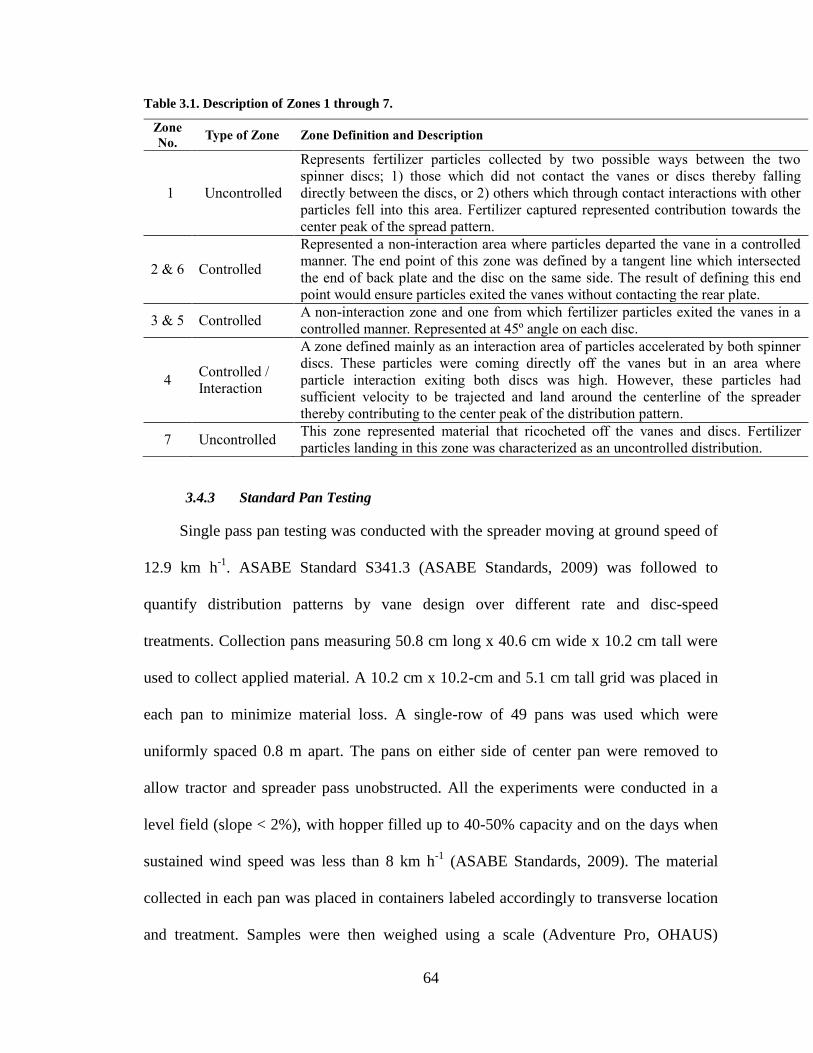
64
Table 3.1. Description of Zones 1 through 7.
Zone
No. Type of Zone Zone Definition and Description
1 Uncontrolled
Represents fertilizer particles collected by two possible ways between the two
spinner discs; 1) those which did not contact the vanes or discs thereby falling
directly between the discs, or 2) others which through contact interactions with other
particles fell into this area. Fertilizer captured represented contribution towards the
center peak of the spread pattern.
2 & 6 Controlled
Represented a non-interaction area where particles departed the vane in a controlled
manner. The end point of this zone was defined by a tangent line which intersected
the end of back plate and the disc on the same side. The result of defining this end
point would ensure particles exited the vanes without contacting the rear plate.
3 & 5 Controlled A non-interaction zone and one from which fertilizer particles exited the vanes in a
controlled manner. Represented at 45º angle on each disc.
4 Controlled /
Interaction
A zone defined mainly as an interaction area of particles accelerated by both spinner
discs. These particles were coming directly off the vanes but in an area where
particle interaction exiting both discs was high. However, these particles had
sufficient velocity to be trajected and land around the centerline of the spreader
thereby contributing to the center peak of the distribution pattern.
7 Uncontrolled This zone represented material that ricocheted off the vanes and discs. Fertilizer
particles landing in this zone was characterized as an uncontrolled distribution.
3.4.3 Standard Pan Testing
Single pass pan testing was conducted with the spreader moving at ground speed of
12.9 km h-1
. ASABE Standard S341.3 (ASABE Standards, 2009) was followed to
quantify distribution patterns by vane design over different rate and disc-speed
treatments. Collection pans measuring 50.8 cm long x 40.6 cm wide x 10.2 cm tall were
used to collect applied material. A 10.2 cm x 10.2-cm and 5.1 cm tall grid was placed in
each pan to minimize material loss. A single-row of 49 pans was used which were
uniformly spaced 0.8 m apart. The pans on either side of center pan were removed to
allow tractor and spreader pass unobstructed. All the experiments were conducted in a
level field (slope < 2%), with hopper filled up to 40-50% capacity and on the days when
sustained wind speed was less than 8 km h-1
(ASABE Standards, 2009). The material
collected in each pan was placed in containers labeled accordingly to transverse location
and treatment. Samples were then weighed using a scale (Adventure Pro, OHAUS)
65
measuring to the nearest 0.01 gm. Mass (g) of the material captured in each pan was
converted to an application rate (kg ha-1
) through division of the pan area (2065 cm-2
).
3.4.4 Physical Properties
An in situ bulk density instrument (Berckes Manufacturing, Canby, MN USA) was
used to estimate the bulk density of potash during tests. Bulk samples were collected at
random from hopper of the spreader during stationary and field tests to determine particle
size and particle density of potash, which were collected in the plastic labeled bags and
sealed afterwards. Camsizer (Model 216753, Retsch Technology GmbH, Germany) was
used to determine the particle size distribution. Five hundred grams of the bulk samples
were used to determine particle size distributions. The Granular Spread Index (GSI);
equation 2.1 was computed to quantify particle size variability. Particle density of the
bulk samples was determined using a gas displacement pycnometer (AccuPyc 1130,
Micromeritics Instrument Corp. Norcoss, GA).
3.4.5 Investigating Particle Behavior
High speed video was utilized to understand how fertilizer particles interacted as
they flowed off the conveyor, across the divider, and onto the spinner discs. These videos
also provided an evaluation means to observe how fertilizer interacted with the vanes and
spinner discs plus visualizing the exit point of particles. The spreader was parked in a
stationary location to collect this video information. The videos were captured at 480
frames per second using high definition video camera (Model No. NEX-FS700U. Sony
Corp. of America, New York, NY USA). Videos were brought back to the lab then

66
analyzed individually to observe how potash particles contacted the vane surface plus
evaluate flow behavior on discs and vanes for all four vane designs.
A discrete element modeling (DEM) software called EDEM® by DEM Solutions
Ltd. (Edinburgh, UK) was used to understand particle behavior including ricocheting and
resulting distribution patterns. This simulation package consists of three main
components; Creator, Simulator and Analyst. The Creator function enables the loading of
CAD (Computer Aided Design) models, characterization of the bulk material or particles,
and selection of the physics to model the spreader and fertilizer materials. The Simulator
provides the actual simulation capabilities which includes the tracking of individual
particles, contact between objects, and calculates this resulting particle behavior. The
Analyst feature enables playback of a simulation along with visualization of resulting
physical behavior such as particle vectors and summary analysis. Due to constraints on
EDEM setup, only Vane 1 was used within this simulation software to directly evaluate
and understand the controlled versus uncontrolled aspect of fertilizer flow and
distribution. A simplified but correctly scaled CAD model was developed to represent the
hopper, conveyor chain, divider, disc and vanes. This CAD representation was uploaded
into the Creator function. Fertilizer particles were modeled as spherical with 6-mm
diameter. Simulations were run with particles isolated between ricocheting and those
distributed by vanes. All particles were tracked with final landing location on the defined
ground noted with single pass patterns for the controlled and uncontrolled aspects of
particle distribution generated. The divider location was changed to determine how these
two patterns were altered. Single-pass patterns were plotted and compared.

67
3.4.6 Data Analysis
For determining the particle exit behavior impacted by the vane design within a
specific disc speed, material concentrated in Zones 1 through 7 were calculated and
statistically analyzed using Analysis of Variance (ANOVA) at a 95% confidence level
within Minitab (v16). For determining the controlled material flow behavior, Zones 1 and
7 were excluded and percentage material concentrations re-calculated for Zone 2 through
6. Multiple comparisons were conducted using Tukey Kramer procedure to analyze the
vane design impact on particle exit behavior off it with the increase in spinner disc speed
and within a specific speed.
Single-pass spread patterns were generated for each treatment by taking the mean
mass of material caught at each transverse position. This data was then used to create the
simulated overlap pass patterns using the progressive method (ASABE Standards, 2009).
These overlap patterns allowed for the mean application rate, standard deviations and
coefficient of variations (CVs) to be calculated for all vane designs in order to evaluate
spread uniformity.
In order to understand distribution uniformity, spread uniformity or CV (%) by
spinner disc speed was plotted against effective spread width for all vanes (fig. 3.5). For
this analysis, the mean single-pass patterns were used to generate the simulated overlap
patterns using the progressive method outlined in ASABE Standard S341.3 (ASABE
Standards, 2009) for spread widths between 10 and 30 m at 5-m increments. The
minimum CV at the maximum spread width was then selected as the effective spread
width at each spinner-disc speed (fig 3.5).

68
Figure 3.5. Example of CV (%) versus effective spread width (m) at the three spinner-disc speeds of 600, 700 and
800 rpm of the fertilizer spreader. The three points indicated the minimum CVs and thereby effective spread
width at the respective spinner disc speed.
Finally, standardized distribution patterns were created by dividing single-pass
patterns by the mean application rate based on the simulated overlap data (Fulton et al.,
2005). These standardized patterns permitted a direct comparison of design and possible
shifts for the various treatments.
3.5 Results and Discussion
3.5.1 Physical Properties
Table 3.2 presents the composite potash (KCl) sample analysis for bulk density,
particle density, mean diameter and Granular Spread Index (GSI). Overall, the GSI was
greater during stationary testing versus pan tests. Mean bulk density for the pan testing
(1153.3 kg m-3
) was found to be greater than stationary testing (1073.2 kg m-3
). Mean
particle density was the same for all tests. However, the mean diameter of 3.0 mm for
potash was greater during pan testing than the stationary tests (2.6 mm).
0
5
10
15
20
25
30
35
10 15 20 25 30
CV
(%
)
Effective Spread Width (m)
600 RPM
700 RPM
800 RPM
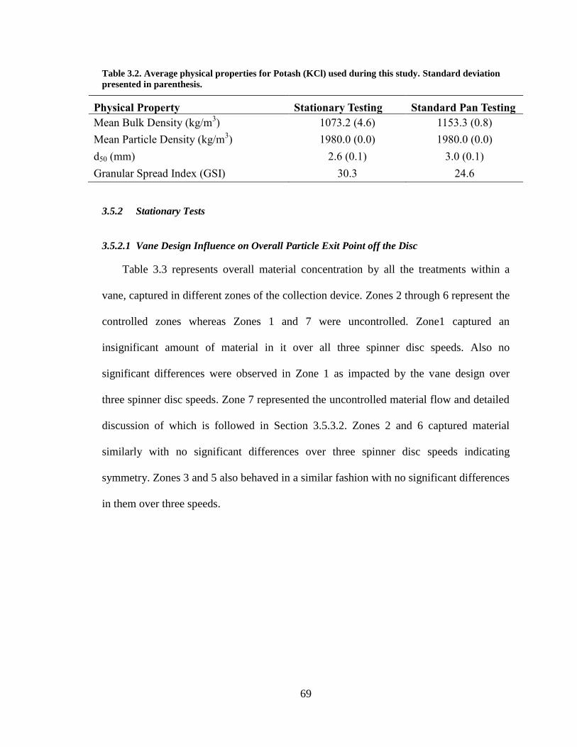
69
Table 3.2. Average physical properties for Potash (KCl) used during this study. Standard deviation
presented in parenthesis.
Physical Property Stationary Testing Standard Pan Testing
Mean Bulk Density (kg/m3) 1073.2 (4.6) 1153.3 (0.8)
Mean Particle Density (kg/m3) 1980.0 (0.0) 1980.0 (0.0)
d50 (mm) 2.6 (0.1) 3.0 (0.1)
Granular Spread Index (GSI) 30.3 24.6
3.5.2 Stationary Tests
3.5.2.1 Vane Design Influence on Overall Particle Exit Point off the Disc
Table 3.3 represents overall material concentration by all the treatments within a
vane, captured in different zones of the collection device. Zones 2 through 6 represent the
controlled zones whereas Zones 1 and 7 were uncontrolled. Zone1 captured an
insignificant amount of material in it over all three spinner disc speeds. Also no
significant differences were observed in Zone 1 as impacted by the vane design over
three spinner disc speeds. Zone 7 represented the uncontrolled material flow and detailed
discussion of which is followed in Section 3.5.3.2. Zones 2 and 6 captured material
similarly with no significant differences over three spinner disc speeds indicating
symmetry. Zones 3 and 5 also behaved in a similar fashion with no significant differences
in them over three speeds.

70
Table 3.3. Overall average of percent material mass (%) measured by zone for each vane design by
spinner disc speed at feed rate of 224 kg ha-1
.
Vane
Disc
Speed
(rpm)
Zone No.
1 2 3 4 5 6 7
Average Mass (%)
1
600
0.8jk
4.7ij
22.0f
22.4ef
22.6ef
6.4hi
21.2f
2 0.6jk
4.6ij
25.1cdef
26.2cde
26.7bcd
4.5ijk
12.2g
3 0.4k
3.8ijk
27.9bc
23.5def
30.4ab
3.7ijk
10.3gh
4 0.4k
4.5ijk
30.4ab
24.2cdef
33.3a
4.1ijk
3.1ijk
1
700
0.6jk
4.0ijk
20.5g
22.8fg
20.9g
5.5i 25.8
bcdef
2 0.8jk
4.0ijk
24.0efg
28.7abcd
25.4cdef
4.0ijk
13.1h
3 0.4k
2.7ijk
27.3bcde
23.3fg
29.2abc
2.5ijk
14.6h
4 0.5k
4.4ij
29.4ab
25.0def
31.7a
4.0ijk
5.0i
1
2
3 800
0.8h
3.1h
17.9f
20.2ef
18.3f
4.3h 35.4
a
0.9h
3.1h
23.5de
28.2bc
25.2cd
3.2h 15.9
f
0.7h
1.7h
25.3cd
26.6bcd
26.7bcd
1.8h 17.3
f
4 0.5h
4.3h
27.5bcd
23.5de
29.7b
3.6h 10.9
g
Means denoted by same letters are not significantly different (level of confidence α = 95%) within a specific disc speed.
3.5.2.2 Controlled Material Flow
Zones 2 through 6 represented controlled material flow on the disc / vanes. Table
3.4 presents the mean mass distribution and comparisons for Zones 2 through 6. It was
indicated that majority of the material concentration was in Zones 3 through 5. Vane 2
captured the greatest amount of material in Zone 4 compared to other three vane designs
irrespective of the spinner disc speed. Vanes 1 and 2 behaved similarly as they received
more material in Zone 4 compared to 3 and 5. Vanes 3 and 4 captured more material in
Zones 3 and 5 compared to Zone 4, indicating more material being pushed out. ANOVA
results indicated no significant differences occurred between the material captured in
Zones 3 and 5 (p>.05) for four vanes at 700 and 800 rpm, indicating they behaved
similarly. However, at 600 rpm, significant differences occurred between Zones 3 and 5
and more material was applied to right side. Zones 2 and 6 showed no significant
differences over all the speeds. Vanes 1 and 2 captured material similarly in Zones 3
71
through 5 at 600 rpm as no significant differences were observed. With the increase in
speed to 700 and 800 rpm for Vanes 1 and 2, differences occurred between Zones 3, 4
and 5. Zone 4 captured more material compared to Zones 3 and 5. Table 3.5 illustrates
the material captured in Zones 2 through 6 and comparisons within specific zones. It
could be noticed that significant differences could be observed on particle exit points off
the vane with the increase in speed and vane design. For Zone 2, Vane 1 captured the
maximum material at 600 rpm with 6.0% and Vane 3 with the least 2.1% at 800 rpm. In
Zone 3, Vanes 3 and 4 showed the maximum material in them followed by Vanes 1 and 2
irrespective of the disc speed. Vane 2 resulted in the greatest amount of material captured
in Zone 4 having 33.9% at 800 rpm compared to other three vane designs. Zone 5
behaved the same like as that Zone 2 with Vanes 3 and 4 capturing more material than
Vanes 1 and 2. Zone 6 behaved similarly like the Zone 2 with Vane 1 capturing the
greatest amount of material 8.3% at 600 rpm and least by Vane 3 showing 2.2% at 800
rpm.
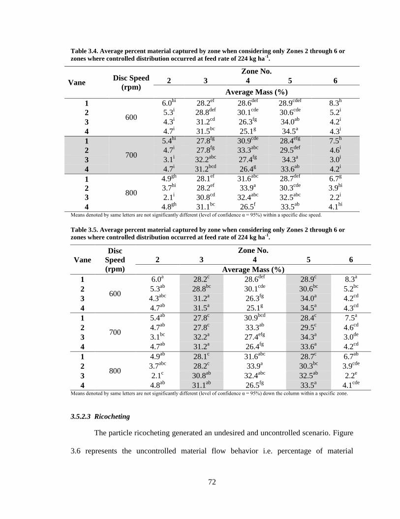
72
Table 3.4. Average percent material captured by zone when considering only Zones 2 through 6 or
zones where controlled distribution occurred at feed rate of 224 kg ha-1
.
Vane Disc Speed
(rpm)
Zone No.
2 3 4 5 6
Average Mass (%)
1
600
6.0hi
28.2ef
28.6def
28.9cdef
8.3h
2 5.3i
28.8def
30.1cde
30.6cde
5.2i
3 4.3i
31.2cd
26.3fg
34.0ab
4.2i
4 4.7i
31.5bc
25.1g
34.5a
4.3i
1
700
5.4hi
27.8fg
30.9cde
28.4efg
7.5h
2 4.7i
27.8fg
33.3abc
29.5def
4.6i
3 3.1i
32.2abc
27.4fg
34.3a
3.0i
4 4.7i
31.2bcd
26.4g
33.6ab
4.2i
1
2
3 800
4.9gh
28.1ef
31.6abc
28.7def
6.7g
3.7hi
28.2ef
33.9a
30.3cde
3.9hi
2.1i
30.8cd
32.4abc
32.5abc
2.2i
4 4.8gh
31.1bc
26.5f
33.5ab
4.1hi
Means denoted by same letters are not significantly different (level of confidence α = 95%) within a specific disc speed.
Table 3.5. Average percent material captured by zone when considering only Zones 2 through 6 or
zones where controlled distribution occurred at feed rate of 224 kg ha-1
.
Vane
Disc
Speed
(rpm)
Zone No.
2 3 4 5 6
Average Mass (%)
1
600
6.0a
28.2c
28.6def
28.9c
8.3a
2 5.3ab
28.8bc
30.1cde
30.6bc
5.2bc
3 4.3abc
31.2a
26.3fg
34.0a
4.2cd
4 4.7ab
31.5a
25.1g
34.5a
4.3cd
1
700
5.4ab
27.8c
30.9bcd
28.4c
7.5a
2 4.7ab
27.8c
33.3ab
29.5c
4.6cd
3 3.1bc
32.2a
27.4efg
34.3a
3.0de
4 4.7ab
31.2a
26.4fg
33.6a
4.2cd
1
800
4.9ab
28.1c
31.6abc
28.7c
6.7ab
2 3.7abc
28.2c
33.9a
30.3bc
3.9cde
3 2.1c
30.8ab
32.4abc
32.5ab
2.2e
4 4.8ab
31.1ab
26.5fg
33.5a
4.1cde
Means denoted by same letters are not significantly different (level of confidence α = 95%) down the column within a specific zone.
3.5.2.3 Ricocheting
The particle ricocheting generated an undesired and uncontrolled scenario. Figure
3.6 represents the uncontrolled material flow behavior i.e. percentage of material

73
ricocheting (overall mean mass distribution percentage by all treatments within a vane,
represented by Zone 7 in table 3.3) for all the vane designs. The design of vane top edge
impacted the level of ricocheting by fertilizer particles thereby amount of uncontrolled
distribution of material. The forward, upward facing top edge at 32° of Vane 1 generated
the highest mean uncontrolled material flow on average 26.6%. Whereas top edge
tapering at 15° facing backwards in Vane 2 resulted in rearwards rotation to the particles
contacting it, thus increased their ability to be picked up the next vane thereby resulted in
reducing overall mean ricocheting to 13.1%. The Vane 3 also generated comparable
overall mean ricocheting of 14.2% as Vane 2 (p>.4568), due to their similar profiles.
The fourth Vane 4, generated the least amount of overall mean ricocheting (6.6%). It was
because that it had an enclosed rectangular U-section and constant height which was also
comparatively less than the other three vane designs. The uncontrolled part of the flow
ranged between 6.6% (Vane 4) and 26.6% (Vane 1) with the maximum difference of 20%
between the upper and the lower values.
3.5.2.4 Impact of Increase in Spinner Disc Speed on Ricocheting
(a) (b)
Figure 3.6. Representation of ricocheting % (i.e. uncontrolled material flow) ± 1 SD for all the four vane shapes,
a. 224 kg ha-1 b. 448 kg ha-1. Means denoted by the same letters are not significantly different (α = 95%).
bc
dedef
f
b
d cd
ef
a
cdcd
de
0.0
10.0
20.0
30.0
40.0
50.0
Vane-1 Vane-2 Vane-3 Vane-4
Ric
och
eti
ng
(%
)
600 rpm
700 rpm
800 rpm
bc
cd
d d
b
cd cd
d
a
cd
b
d
0.0
10.0
20.0
30.0
40.0
50.0
Vane-1 Vane-2 Vane-3 Vane-4
Ric
och
eti
ng
(%
)
600 rpm
700 rpm
800 rpm

74
The results indicated that as disc speed increased, so did the fertilizer collected,
indicating increased ricocheting with disc speed. All vane designs exhibited statistically
significant results for ricocheting in Zone-7 (p<.0001). It was observed that as material
concentration in Zone-7 increased for all vane designs, the percent of potash collected in
the remaining six zones decreased relatively. For all spinner disc-speeds, Vane 1
generated the maximum ricocheting, whereas Vane 4 resulted in the least. The results
indicated that increase in feed rate did not significantly impact (p>.05) the concentration
of material captured within different zones however, the increase in spinner disc speed
did significantly impact distribution between zones (table 3.3). The Vane 1 generated the
highest level of ricocheting ranging between 20.2% at 600 rpm up to 34.5% at 800 rpm.
Vane 2 maintained consistent level of ricocheting; 11.5% at 600 rpm, 12.9% at 700 rpm
and 14.8% at 800 rpm. Vane 3 generated 8.1%, 13.8% and 20.7% at 600, 700 and 800
rpm. The Vane 4 had the lowest ricocheting ranging from 4.6% at 600 rpm, 5.8% at 700
rpm and 9.4% at 800 rpm. The increase in spinner disc speed increased ricocheting. On
increasing the disc speed from 600 to 700 rpm; 25.5%, 13.8%, 70.7% and 27.0% increase
in ricocheting was observed for Vanes 1, 2, 3 and 4. Whereas, an increase of 71.0%,
30.5%, 156.0% and 105.7% was generated in ricocheting on increasing the disc-speed
from 600 to 800 rpm. The concentration of material captured in the Zones 1 and 4
determined vane contribution to the center peak of spread distribution pattern (table 3.3).
Less than 1% of potash was captured in Zone-1 for all vane designs, indicating little
contribution to the center peak and overall pattern. Zones 3 and 5 for Vanes 3 and 4,
received more material in comparison to Zone-4 representing that more material was

75
pushed on the outer ends in spread distribution pattern indicating reduced center peak of
spread distribution pattern.
3.5.3 Distribution Pattern Make-Up
The EDEM simulation results provided clarification that two unique distributions
existed for this spreader. The two patterns were superimposed on each other; controlled
and uncontrolled (fig. 3.6). The controlled flow pattern was desired and could be altered
using known methods for setting the divider, vane angle and disc speed. The uncontrolled
component of material distribution was primarily caused by ricocheting off the vanes and
could not be altered through hardware adjustments. It caused material application directly
behind the spreader along with increasing the center peak of the spread pattern, the
undesired one. While conducting the static tests for the single-pass spread patterns, an
interesting observation was made that regardless of altering the flow divider position, the
spread pattern did not change shape. Therefore single-pass pattern was divided into two
individual patterns. The one pattern consisted of potash landing up to 4.88 m traversely
behind the spreader (fig. 3.7) and termed the uncontrolled aspect of distribution. The
other called was termed the controlled distribution and is desired. Simulation results
indicated that the center peak never changed regardless of the divider adjustments thereby
representing ineffectiveness of the divider adjustments for changing the spread pattern
shape. However, the controlled pattern responded to adjustments made in divider
position.

76
Figure 3.7. Depiction of the two spread patterns which make up the overall single-pass spread pattern based on
EDEM simulations. One pattern represents the controlled material distribution and the other uncontrolled.
3.5.4 Standard Pan Tests
3.5.4.1 Standardized Distribution Pattern Analysis
Figure 3.8 represents the mean standardized distribution patterns for all the vane
designs. The spread distribution pattern varied by vane design. The trends obtained at
both the feed rates were comparable with minor shifts on either edge. Increasing the feed
rate to 448 kg ha-1
, the center peak also increased. The reason was that ricocheting caused
the particles to be applied along the spreader centerline (+/- 2.3 m). Vane 1 resulted in
the highest center peaks in comparison to other vanes due to reason that it resulted the
greatest ricocheting over three disc speeds compared to other three vane designs as
presented in Table 3.3. Vane 1 generated 21.2%, 25.8% and 35.4% ricocheting over disc
speeds of 600, 700 and 800 rpm which were significantly higher than the other three vane
designs (Table 3.3). It was because that when particles contacted the top edge of Vane 1,
particle ricocheting off the vane occurred thereby resulting in high center peaks. On
comparing Vane 1 with 2, Vane 2 had a smaller center peak (fig. 3.8) and more effective
spread width (Table 3.6). The reason was that Vane 2 had 15° tapered top edge facing

77
backwards such that when the particles contacted it, rearward rotational motion was
generated thereby increasing their ability to be picked up by the next vane. Also the
material captured in Zones 3, 4 and 5 for Vane 2 was greater compared to Vane 1 (Table
3.4) indicating more controlled material behavior in Vane 1 than Vane 2. Due to
reduction in center peak, more material was pushed to the outer edges of the spread
distribution pattern thus indicating more effective spread width. As disc speed increased,
the peaks on either edge reduced while the center peak increased in magnitude. This can
be explained on the basis that with increase in disc speed particle ricocheting off the
vanes increased, which caused greater material concentration to fall along the centerline
behind the spreader and thus reduced concentration on the either edges.
(a) (b) (c)
Figure 3.8. Mean average standardized distribution patterns for all vanes; designated as 1, 2, 3 and 4 at feed rate
of 224 kg ha-1 over spinner disc speeds of a) 600 rpm, b) 700 rpm and c) 800 rpm. Each curve in the graph
represents mean of three replications. Transverse location represents the position of pans on the spread width, 0
represents the point of travel of the spreader with negative points on the left hand side of the spreader and
positive points on right hand side of the spreader.
3.5.4.2 Impact of Vane Design on Effective Spread Width
The vane shape impacted the fertilizer particle interaction on vane-disc assembly
and ultimately resulting spread pattern and effective spread width. The disc speed was the
primary parameter which controlled the spread width but vane design also impacted the
maximum spread width for a fertilizer product. The effective spread width varied by vane
0.0
0.6
1.1
1.7
2.2
-18.5 -9.3 0.0 9.2 18.5
Sta
nd
ard
ize
d D
istr
ibu
tio
n
Pa
ttern
Tranverse Location (m)
Vane-1Vane-2Vane-3Vane-4
0.0
0.6
1.1
1.7
2.2
-18.5 -9.3 0.0 9.2 18.4Sta
nd
ard
ized
Dis
trib
uti
on
P
att
ern
Tranverse Location (m)
Vane-1Vane-2Vane-3Vane-4
0.0
0.6
1.1
1.7
2.2
-18.5 -9.3 0.0 9.2 18.4Sta
nd
ard
ize
d D
istr
ibu
tio
n
Patt
ern
Tranverse Location (m)
Vane-1Vane-2Vane-3Vane-4

78
design on spinner-disc speeds of 600, 700 and 800 rpm. The effective spread width
increased with spinner disc speed for all the vane designs as shown (fig. 3.8). For the
Vanes 1, 2, 3 and 4, an increase of 16.7% in the effective spread width was observed on
increasing disc-speed from 600 to 700 rpm. A 7.1% gain was observed on increasing the
speed from 700 to 800 rpm for vanes 1, 2 and 3. However the Vane 4 had the greatest
increase of 14.3% in effective spread width with spinner disc-speed increase from 700 to
800 rpm. It was because of enclosed rectangular U-section in Vane 4 and reduced exit
height in comparison to other vanes, due to which the velocity vector of exiting particles
had greater magnitude of horizontal component than the vertical component which
assisted in projecting the particles to the maximum distance thus the greatest effective
spread width. It was observed that at disc speed of 600 rpm, effective spread width of
18.3 m and 21.3 m at 700 rpm was obtained for all vane designs. The point of interest
was at 800 rpm as the trend obtained was not the same, 22.9 m effective spread width
was generated by Vanes 1, 2 and whereas 24.4 m for Vane 4.
Table 3.6. Impact of increase in spinner disc speed on effective spread width for the Vanes 1, 2, 3 and
4.
Disc Speed
(rpm)
Vane
1,2 and 3 4
-------------------Spread Width (m) -------------------
600 18.3 18.3
700 21.3 21.3
800 22.9 24.4
3.5.4.3 Vane Design Impact on Spread Uniformity
Figures 3.9 and 3.10 represent the impact of vane design on spread uniformity and
plots for which were generated using simulated overlap analysis. The spread uniformity
varied over the effective spread width by vane design. It was found that Vane 2 resulted

79
in the lowest and most consistent spread uniformity over all disc speeds. Spread
uniformity improved with spinner disc speed for both Vane 3 and 4. For Vane 1, spread
uniformity deteriorated the most with increase in disc speed. At 800 rpm for Vane 1, the
CV versus spread width indicated that spread uniformity did not follow the expected
trend of shifting the curve to the right as disc speed increased. Around 20 m, this curve
somewhat leveled out and quickly increased and there was not much offset to the right
for the 800 rpm curve versus 700. This result was not found in the other three vanes.
One explanation for this was the 35% or more level of ricocheting caused by Vane 1 at
this high disc speed deteriorating the spread uniformity.
Figure 3.9. Plot of spread uniformity (CV; %) versus effective spread width for Vane 1 (left) and Vane 2 (right)
over different disc speeds.
Figure 3.10. Plot of spread uniformity (CV; %) versus effective spread width for Vane 3 (left) and Vane 4 (right)
over different disc speeds.
10 15 20 25 30
CV
(%
)
Spread Width (m)
600 RPM
700 RPM
800 RPM
10 15 20 25 30
CV
(%
)
Spread Width (m)
600 RPM
700 RPM
800 RPM
10 15 20 25 30
CV
(%
)
Spread Width (m)
600 RPM
700 RPM
800 RPM
10 15 20 25 30
CV
(%
)
Spread Width (m)
600 RPM700 RPM800 RPM600 RPM

80
3.5.4.4 Particle Flow Behavior
The high speed video analysis provided insight which confirmed the level of
ricocheting varied by vane design. Most noticeable was the high level of ricocheting by
Vane 1 (fig. 3.11) with a noticeable reduction for Vanes 2, 3 and 4. The high speed
videos indicated that the ricocheting was primarily due to fertilizer flow intersecting the
top edge of the vane with minimal resulting from bouncing off the spinner-disc. For all
vane designs most of the material was flowing along vane bottom at a height of carriage
bolts above the vane base. The bolt heads influenced the minimum exit height of particles
as they left the vane. The bolt heads located at the bottom of the vane mounting it to the
disc, kept material flow above the bolt heads as particles flew across the vane face. The
open end profile Vanes – 1, 2 and 3 tended to generate greater magnitude of vertical
velocity vector component (fig. 3.12) thus reduced effective spread width whereas the
Vane 4 had an enclosed rectangular cross section (U-shaped) which reduced the exit
height of particles while increasing the horizontal, exit velocity vector component thereby
increasing the maximum distance travelled and effective spread width (fig. 3.11). As the
particles were not always intercepted immediately by the vanes, they acquired some
initial velocity through collisions with the disc, before the succeeding vane caught them.
Furthermore, when potash particles contacted the top edge of vane, particle ricocheting
off was observed.
A significant amount of material was found to be ricocheted off by the vanes as
compared to the discs. It was observed that particles contacting the vane edges had more
lateral and vertical velocity in comparison to particles contacting the discs. The backward
tapered top edge of Vane 2 generated a rearward rotational velocity for the particles
contacting it. The result was that these particles would fall back onto the disc and

81
intercepted in the next vane thus increased the vane efficacy. The particles that contacted
the disc only did not travel far thereby being applied directly behind the spreader. The
Vane 4 was the most aggressive design in terms of describing the interaction of fertilizer
particles with the vane on initial contact. This interaction generated more ballistics
resulting in fertilizer particles breaking into fine versus the other three vane designs.
Figure 3.11. Illustration of material flow and ricocheting off Vane 1.
Figure 3.12. Material flow off Vane 3 (left) versus Vane 4 (right). Note the absence of ricocheting for Vane 4.
3.6 Summary
Two types of fertilizer flow were discovered generating two distinct spread patterns
superimposed to form the overall spread pattern; a) controlled and b) uncontrolled
material flow. The controlled material was desirable and could be regulated making
through hardware adjustments such as flow divider position, gate height and disc/vane
design. Whereas the uncontrolled flow caused material application directly behind the
spreader as it was difficult to manage. This study showed that the level of ricocheting was
Controlled material flow
Ricocheting
Material Flow
Vane-3
Material Flow
Vane-4

82
significantly impacted by top edge of the vane thereby impacting the amount of
uncontrolled material off the vanes. The level of ricocheting was significantly impacted
by top edge design of vane. The forward upward facing top edge of the Vane 1 generated
the maximum overall mean ricocheting of 26.6% when the particles contacted it.
However, the rearward facing top edge of the Vane 2 resulted in backward rotation on the
particles contacting it thereby reducing overall mean ricocheting in half (13.1%). Due to
similarity in the profiles of Vanes 2 and 3, Vane 3 generated comparable overall mean
ricocheting 14.2% to Vane 2. The Vane 4 generated the least ricocheting of 6.6%.The
ricocheting increased with spinner disc speed. The result of ricocheting was that these
particles were applied along the spreader centerline thus increasing the center peak of
spread distribution pattern. Particle exit behavior depended on the vane shape as Vanes 3
and 4 resulted in more material concentration in Zones 3 and 5 compared to material
captured by Vanes 1 and 2, thereby indicating more material being pushed out by
enclosed U-sections of Vanes 3 and 4 than open profile Vanes 1 and 2. The controlled
material exit behavior represented that Zones 2 and 6 behaved similarly and likewise
Zones 3 and 5. Vane 2 resulted in consistent distribution uniformity across all disc
speeds. The effective spread width increased with the spinner disc speed. The increase in
spinner-disc speed from 600 to 700 rpm increased the effective spread width by 3.0 m
regardless of the vane design. Vane 4 at 800 rpm, generated the greatest effective spread
width of 24.4 m compared to 22.9 m obtained for Vanes 1, 2 and 3. Shortened vane exit
height resulted in greater magnitude of the horizontal velocity vector thereby creating a
wider effective spread width. In conclusion, vane design impacted spread uniformity that
can affect long-term soil fertility levels if poor distribution occurs over time.

83
Chapter 4 COMPARISON OF CHEMICAL VERSUS PHYSICAL METHODS
FOR MEASURING NUTRIENT CONCENTRATION
4.1 Abstract
Blended fertilizers are commonly used in the US as a soil/crop nutrient source using
dual disc spinner spreaders. However, due to variation in physical properties, there can be
issues of non-uniform spread which could lead to deviation from the desired nutrient
pattern. Therefore, the objective of this study was to determine nutrient concentration
across the swath while applying a 10-26-26 blend using dual disc spinner spreader. In
order to determine the phosphorous oxide (P2O5) and potassium oxide (K2O)
concentration within a fertilizer sample, two methods were used; a) chemical and b)
manual separation. The P2O5 and K2O concentration data obtained through the chemical
method was consistently lower than the physical method. However, the nutrient
concentration patterns for P2O5 and K2O generated similar trends for both methods by an
average difference factor of 1.15.
4.2 Introduction
The fertilizers are essential for crop production. Basically there are two types of
fertilizers a) Single Product b) Blends. Single product fertilizers such as urea (46-0-0),
potash (0-0-60) supply only one nutrient however the blends like 13-13-13, 17-17-17 can
provide all three macronutrients N, P2O5 and K2O at once as per the crop and soil
requirements. Therefore use of blended fertilizers overcomes the number of multiple
84
passes that one has to make while using single product fertilizers. The dual disc spinner
spreaders being simple and cost effective are commonly used to spread granular
fertilizers. Over the past few years, spreader manufacturers have increased the spread
widths up to 21-30 m. With the increase in spread widths, the blended fertilizer
application can promote risk of segregation due to variation in physical properties of the
constituents of blend. The non-uniform fertilizer application coupled with repeated field
traverses over years using automatic guidance can cause streaking in the field. Therefore
it is essential to determine nutrient concentration across the swath after spreading the
fertilizer to look for any deviations from the target. Two methods were implemented for
determination of nutrient concentration; chemical analysis conducted within a lab and a
physical method. The specific objectives of this investigation were to 1) determine
nutrient concentration across the swath using chemical and physical methods and 2)
compare and contrast chemical and physical methods.
4.3 Methodology
4.3.1 Chemical Method
The fertilizer samples collected in pans after spreading the blend 10-26-26 using
dual disc spinner spreader, were ground using a mortar and pestle. The mortar and pestle
were thoroughly cleaned after grinding each sample. After grinding, samples were put
back in their respective bags and sealed. Standard Inductively Coupled Argon Plasma
Spectrophotometer (ICAP) was used to determine the P2O5 and K2O concentration of
each sample. A 0.5 g sample was required to determine P2O5 and K2O. The pans near the
far ends on both sides of swath received very less material and weighed lower than 0.5 g.
85
Due to this limitation, the chemical analysis was conducted only for the inner portion of
the swath; -10.7 to 9.1 m.
The ground fertilizer samples were extracted with ammonium citrate at a pH of 7.
The ammonium citrate was prepared using Di-sodium EDTA (Ethylene Di-amine Tetra
Acetic Acid) and Di-basic ammonium citrate. The 0.5 g of fertilizer samples were
weighed and put in labeled jars corresponding to pan number with jars sealed tightly.
Afterwards, 100 ml of ammonium citrate was added to each jar and sealed again. In order
to extract the samples, sealed jars were placed in shaker water bath (Magni Whirl
Constant Temp Bath US Patent No. 2813, Blue M-B-2729-Q-189) at 65°C for a duration
of one hour while shaking at 200 rpm. The shaker was designed such that jar contents
continuously bathe the inner surface of jar in hot water. Jars were then removed from the
shaker and cooled to 20-250C in the laboratory at ambient temperature. The extracted
samples were filtered in flasks using Whatman#42 filter paper. Distilled water was then
added to each flask to bring the total volume up to 100 ml. The flasks tops were sealed
using plastic wraps and then turned upside down for thoroughly mixing the samples.
Then 10 ml of these samples were then placed in vials and labeled accordingly. The
samples collected in vials were then run on the ICAP for determining the percentage
concentration of P2O5 and K2O. Afterwards the jars, vials and flasks were washed in
distilled water, then in a hydrochloric acid bath and again washed in distilled water twice
to thoroughly clean and remove any leftover samples.
The chemical method involved extractions using ammonium citrate at 65ºC while
maintaining 200 rpm of water bath. It included use of expensive chemicals and time
constraint due to extraction of maximum six possible samples in water bath. Also the

86
original samples could not be retained for future reference while using chemical method.
So manual separation of DAP and potash was done and percent nutrient concentration
determined for phosphorous oxide (P2O5) and potassium oxide (K2O) as detailed in the
following section 4.3.2.
4.3.2 Physical Method
The physical method involved manually separating DAP and Potash particles of the
blend (10-26-26) samples. The cubical shaped containers were constructed using paper
cardboard with their tops open. The paper sheets were folded such as to make rectangular
plates with edges on all four sides to hold the fertilizer sample and a hole in middle to
allow the separation of DAP from potash. The fertilizer sample collected in a pan was put
in a plate, then DAP and potash separated using wooden bars. Separated DAP and potash
particles were weighed individually. In order to determine the percentage concentration
of phosphorous oxide (P2O5) and potassium oxide (K2O), equations 4.1 and 4.2 were
generated and used.
(4.1)
where
P2O5 = percentage of phosphorous oxide
a = mass of DAP at a given pan location (g)
c = total mass of sample collected at a given pan location (g)
0.46 = Phosphorus Oxide (46%) in DAP
87
(4.2)
where
K2O = percentage of potassium oxide
b = mass of potash at a given pan location (g)
c = total mass of sample collected at a given pan location (g)
0.60 = Potassium Oxide (60%) in Potash
4.3.3 Inequality Ratio
The inequality ratios were calculated in an attempt to reduce the differences
between physical and chemical methods. The inequality ratios were calculated using the
sum total of nutrient concentrations for P2O5 and K2O across the swath for the physical
method divided by the sum obtained through the chemical method.
4.3.4 Statistical Analysis
A statistical analysis was conducted to compare and contrast the chemical and
physical methods. The mean, standard deviation and percentage differences were also
calculated for comparisons.
4.4 Results
Table 4.1 represents the percent nutrient concentration values generated for
P2O5and K2O by chemical method. A and B indicated the results obtained by two
different people running the same sample using the chemical analysis. The target nutrient
concentration was 26% for P2O5and K2O. A and B, both obtained similar results which
were lower than the expected concentration of 26% for P2O5and K2O respectively. The

88
chemical method generated consistently lower nutrient concentrations for P2O5and K2O
versus the physical method. Table 4.2 confirmed the low nutrient values for P2O5and K2O
than the target concentration of 26%.
Table 4.1. Results of nutrient concentration conducted by two different people (labeled A and B) in
the lab on the same sample using the chemical method.
Fertilizer Sample
(10-26-26)
---------- A ---------- ---------- B ---------
P2O5 (%) K2O (%) P2O5 (%) K2O (%)
1 22.2 20.2 23.1 20.5
2 21.6 19.7 22.6 20.3
Table 4.2. Nutrient concentration results for running three samples twice using the chemical
method.
Fertilizer Sample
(10-26-26)
----- Replication-1 ------ ----- Replication-2 -----
P2O5 (%) K2O (%) P2O5 (%) K2O (%)
1 23.1 19.3 22.8 18.9
2 21.8 20.1 21.5 20.3
3 22.5 21.7 21.7 22.4
The differences for P2O5 between two methods ranged between 3.6-4.3% at feed
rate of 224 kg ha-1
and 1.8 - 3.2% for 448 kg ha-1
(Table 4.3). Similarly for K2O, the
observed differences between two methods ranged between 3.9 - 4.6% at 224 kg ha-1 and
1.8 - 2.6% over 448 kg ha-1
. P2O5 concentration for the chemical method was 4.3%, 3.6%
and 3.6% lower than the physical data at a feed rate of 224 kg ha-1
and spinner disc
speeds of 600, 700 and 800 rpm, respectively. At a feed rate of 448 kg ha-1
, P2O5
concentration obtained through the chemical method was 3.2%, 4.0% and 1.8% lower
than the physical data at 600, 700 and 800 rpm, respectively. The chemical method was
found to be more variable in determining nutrient concentration compared to the physical
method. In general, the standard deviations for the chemical method were higher in
magnitude compared to physical method (Table 4.3).

89
Table 4.3. Mean P2O5 and K2O concentrations determined using the chemical and physical methods
with standard deviation presented in parenthesis. The difference between the two methods is also
presented in the last two columns.
Feed
Rate
(kg ha-1
)
Disc
Speed
(rpm)
Chemical Method
(%)
Physical Method
(%)
Difference
between the two
methods (%)
P2O5 K2O P2O5 K2O P2O5 K2O
224
600 21.9 (2.7) 22.0 (3.1) 26.2 (2.4) 25.9 (3.0) 4.3 3.9
700 22.3 (2.7) 23.0 (2.7) 25.9 (2.2) 26.2 (2.9) 3.6 3.2
800 21.8 (2.3) 22.3 (3.2) 25.4 (1.4) 26.9 (1.8) 3.6 4.6
448
600 23.5 (2.8) 22.6 (3.1) 26.7 (2.7) 25.2 (3.6) 3.2 2.6
700 22.1 (1.6) 24.1 (2.3) 26.1 (1.9) 26.1 (2.4) 4.0 2.0
800 24.2 (2.0) 24.2 (2.1) 26.0 (1.5) 26.0 (2.0) 1.8 1.8
At a feed rate of 224 kg ha-1
, the K2O concentration data was 3.9%, 3.2% and
4.6% lower than the physical data over 600, 700 and 800 rpm, respectively. For a feed
rate of 448 kg ha-1
, 2.6%, 2.0% and 1.8% variations were observed between the chemical
and physical data at 600, 700 and 800 rpm, respectively. As chemical method generated
consistently lower values compared to physical method, mean equality ratio of 1.15 was
calculated and multiplied with original chemical data to result final chemical data as
presented in figure 4.1. It can be noticed that trends obtained between original chemical,
final chemical and physical values were similar.

90
(a) (b)
(c) (d)
Figure 4.1. Comparisons between original chemical, final chemical and physical data for P2O5 and K2O at two
feed rates 224 kg ha-1 (a and b) and 448 kg ha-1 (c and d).
4.5 Summary
Compared to manually separating individual constituents, the chemical analysis
generated consistently lower nutrient concentration values for P2O5 and K2O. P2O5 and
K2O concentration values followed similar trends with an average difference factor of
1.15 existing between the two methods.
10.0
20.0
30.0
40.0
50.0
-12.0 -9.0 -6.0 -3.0 0.0 3.0 6.0 9.0
P2O
5%
Transverse Location (m)
Final ChemicalOriginal ChemicalPhysical
10.0
20.0
30.0
40.0
50.0
-12.0 -9.0 -6.0 -3.0 0.0 3.0 6.0 9.0
K2O
%
Transverse Location (m)
Final ChemicalOriginal ChemicalPhysical
10.0
20.0
30.0
40.0
50.0
-12.0 -9.0 -6.0 -3.0 0.0 3.0 6.0 9.0
P2O
5%
Transverse Location (m)
Final ChemicalOriginal ChemicalPhysical
10.0
20.0
30.0
40.0
50.0
-12.0 -9.0 -6.0 -3.0 0.0 3.0 6.0 9.0
K2O
%
Transverse Location (m)
Final ChemicalOriginal ChemicalPhysical
91
Chapter 5 POTENTIAL OF FERTILIZER SEGREGATION DURING
APPLICATION USING SPINNER-DISC SPREADER
5.1 Abstract
Granular blended fertilizers are commonly applied using spinner-disc spreaders in the
U.S. with spread widths between 60 and 100 ft. Today, uniformity of spread is important
as growers and custom applicators attempt to implement site-specific management and
utilize GPS-based guidance systems which permit equipment to follow the same field
traverses over time. However, variation in physical properties of the N, P and K
components of blended fertilizers make it difficult to spread them uniformly plus
segregation could occur. Therefore, an investigation was conducted to understand the
potential of fertilizer segregation during application with a spinner disc spreader. A series
of standard pan tests were performed for evaluating nutrient distribution for a blended
fertilizer (10-26-26). Treatments included two feed rates (224 and 448 kg ha-1
) and three
spinner disc speeds (600, 700 and 800 rpm). Results indicated that application of the
blended fertilizer resulted in non-uniform spread of the nutrients. Distinct nutrient
patterns were generated for the different constituents; “W” shaped for P2O5 and “M” for
K2O regardless of feed rate and spinner disc speed. An increase in spinner disc speed
widened the maximum transverse distance travelled by particles however it was not equal
in magnitude for DAP and potash highlighting segregation. The level of segregation
increased with spinner disc speed (p<.05) but not with feed rate (p>.05).
92
5.2 Introduction
Spread distribution uniformity is a key goal when applying fertilizers to obtain
maximum crop yield and minimize environmental issues. Fertilizers are available as
single product such as potash (0-0-60) and urea (46-0-0) or in blended forms (e.g. 13-13-
13; 20-20-20; 5-20-20). Blended fertilizers have several advantages compared to single
products. Bulk blending helps in providing a practical and economical way to produce
crops therefore blends constitute a total of 70% of the total solid fertilizers sold in the
U.S. (Formisani, 2005). Blended fertilizer application is economical as it helps in
reducing the number of passes across fields in comparison to single product fertilizer
application (Yule and Pemberton, 2009) where multiple passes might be required. This
practice of using blended fertilizers avoids excess nutrients, which potentially could enter
the environment (Miserque et al., 2008). Even though blended fertilizer application has
several advantages, segregation of individual components during handling or spreading is
a potential problem (Hoffmeister et al., 1964; Hofstee and Huisman, 1990; Bridle et al.,
2004; Bradley and Farnish, 2005). Segregation represents the un-mixing of fertilizer
constituents (e.g. N, P2O5, K2O) during handling and field application (Hoffmeister et al.,
1964; Achorn, 1984). Blended fertilizer can consist of different particle sizes along with
different shapes and densities which can cause segregation (Hart, 1998) and segregation
is the primary cause of uneven distribution in the field. A fertilizer blend may be initially
mixed such that the individual constituents are uniform throughout the volume. However,
segregation occurs due to separation of particles into distinct zones by particle size, shape
and density (Maynard, 2012). Physical segregation of blended fertilizers may result in
different distribution patterns for individual nutrients varying rates over the applied areas
(Jensen and Pesek, 1962a).

93
Various factors exist that cause segregation. A number of researchers have
conducted studies in order to determine the effect of particle size on segregation during
spreading of fertilizers. Bridle et al. (2004), Bradley and Farnish (2005) and Tang and
Puri (2007) indicated that segregation occurred during spreading due to differences in
particle sizes of the blended fertilizer. Williams (1976) suggested that a blend with a
mean particle diameter larger than 100 µm and variation of more than 30% can cause
segregation. Miserque et al. (2008) found that the variation in particle sizes caused
segregation as bigger particles tended to be thrown further across the swath while smaller
ones landed directly behind the spreader during spreading. They also concluded that
variation in particle size and density are the major parameters affecting spread patterns.
In other studies (Hofstee and Huisman, 1990; Miserque and Pirard, 2004), it was found
that blends should be produced with similar particle size or 10% variation or less in
particle size to reduce the segregation. Pircon et al. (1964) suggested that compaction can
be one way to reduce segregation. Secondly they recommended that if round shaped
particle are selected for the blend, segregation could be reduced as they form rhombic
array.
The shape of fertilizer particles has been found to have minimum effect on
segregation (Hoffmeister et al., 1964; Miserque and Pirard 2004; Miserque et al., 2008.
However, Pircon et al. (1964) detemined that particle size contributed towards
segregation because friction factor is intimately related to the particle size. They also
indicated that fertilizer particles with similar friction factors reduce segregation in
blended products. The particles having irregular shape are more prone to segregation than
spherical particles (Tang and Puri, 2007). Jha et al. (2008) reported that percent

94
segregated fines were higher (59%) for angular particles as compared to spherical
particles. Spread pattern and segregation of fertilizer particles also depend on their
breaking strength (Hofstee, 1992). He also reported that urea had a breaking force of less
than 15 N. Consequently, urea was not sufficiently hard enough resulting in particle size
reduction, sometimes to powder, when impacting the spinning disc and vanes. This
resulted in smaller fines and powder particles landing directly behind the spreader.
5.3 Sub-objectives
The present research is focused on understanding potential segregation of granular
fertilizer using spinner disc spreaders. The objectives of this study were to 1) compare
and contrast, nutrient distribution patterns with increase in feed rate and spinner disc
speed for a blended fertilizer using a spinner-disc spreader, and 2) evaluate the impact of
increase in feed rate and spinner disc speed on level of segregation for a blended fertilizer
across the swath width.
5.4 Materials and Methods
A commercially available spinner-disc spreader (fig. 3.1; Chandler Equipment
Company, Gainesville, GA USA) was used in this study. Hydraulically controlled dual
rear spinner discs and stainless steel mesh conveyor chain were standard on the spreader.
Four equally spaced vanes (Vane 2 featuring a tapered backwards top-edge at 15° as
described in fig. 3.2a and 3.2b of Chapter-3) were mounted on discs. The reason behind
using Vane 2 was that it reduced the ricocheting by 50% compared to the Vane 1 being
supplied by the manufacturers on the spreaders. Also, Vane 2 resulted in consistent
lowest CVs compared to the other 3 vane designs. The spinner discs were concave in

95
shape, 0.60 m in diameter, 0.04 m height and nominal a 9.3 degree exit angle at the
periphery. Proportional hydraulic valves (Brand Hydraulics, Omaha, NE) with pulse
width modulation maintained hydraulic flow for conveyor chain and spinner discs. A
John Deere 7230 tractor was used to pull the spreader and was equipped with a Raven
SmartTrax guidance system using RTK correction and an Envizio Pro display (Raven
Industries Sioux Falls, SD USA). The Envizio Pro and associated rate controller provided
conveyor and spinner disc speed management based on user input parameters. The flow
divider on the rear of spreader helped in splitting material flow and control delivery
location onto each disc.
Treatments included two feed rates of 224 and 448 kg ha-1
and spinner disc speeds
of 600, 700 and 800 rpm. Standard pan testing was conducted at the EV Smith Research
Center, Shorter, AL using a 10-26-26 blend following ASABE Standard S341.3 (ASABE
Standards, 2009) for determining spread distribution patterns and uniformity. Ground
speed was kept constant at 12.9 km h-1
for all treatments. The spreader hopper was
filled to 40-50% capacity and experiments were conducted on days when sustained wind
speed was less than 8 km h-1
(ASABE Standards, 2009). The test site was flagged for 49
uniformly spaced pans at 0.8 m increments on a level field (slope <2%). Pans on either
side of the center pan were removed to allow the tractor pass unobstructed. Collection
pans had dimensions of 50.8-cm long x 40.6-cm wide x 10.2-cm tall with a 5.1-cm tall
and 10.2 cm x 10.2-cm grid. Material collected in pans was placed in labeled bags and
sealed after weighing (Adventure Pro, OHAUS) for calculating application rates and
computing single-pass and simulated overlap patterns.

96
5.4.1 Determination of Physical Properties of Fertilizers
Bulk samples were collected at random in plastic bags from the spreader hopper
during tests. An in-situ bulk density instrument (Berckes Manufacturing, Canby, MN)
was used to determine bulk density of the blend 10-26-26. Particle size analysis was
carried out on 500 g samples using a Camsizer (Model 216753, Retsch Technology
GmbH, Germany). Particle size was reported as d16, d50 and d84 (dx: x is the fraction
weight passing the sieve of mesh d) to computed the Granular spread index (GSI).
5.4.2 Data Analysis
Mass of material collected in the collection pans was converted to an application
rate (kg ha-1
) and was calculated using the mean mass of material collected in pans
for each transverse position. The progressive method (ASABE Standards, 2009) was used
to generate simulated overlap patterns. The mean application rate, standard deviation and
coefficient of variation (CV) were also calculated using the simulated overlap passes.
Standardized mass distribution patterns were plotted by dividing average application rate
from the simulated overlap passes (Fulton et al., 2005) for each transverse position.
Standardization helped comparing and contrasting patterns for different application rates.
At a 95% confidence level, an analysis of variance (ANOVA) was conducted using
the general linear model (GLM) procedure with SAS (Statistical Analysis Software, SAS
Inst., NC, 9.2) to determine statistical differences between nutrient concentration values
for P2O5 and K2O. The ANOVA analysis compared nutrient concentration at feed rates
of 224 kg ha-1
and 448 kg ha-1
over disc speeds of 600, 700 and 800 rpm. Multiple
comparisons were also carried out using Tukey Kramer procedure at the 95% confidence
interval to determine if differences existed for all combinations.

97
5.5 Results and Discussions
5.5.1 Fertilizer Physical Properties
Table 5.1 presents the physical properties measured for the bulk samples collected
during testing. The granular spread index (GSI) for potash was the greatest (22.8)
compared to di-ammonium phosphate-DAP (14.2) indicating greater size variability in
potash. GSI for the blend was 19.1. GSI values of greater than 10 are considered to cause
segregation (Miserque and Pirard, 2004), therefore DAP and potash generated possibility
of segregation due to greater GSI’s than 10. DAP had the greatest median diameter (d50)
of 3.2 mm followed by potash and the blend (d50=3.0mm). Also DAP particles were more
spherical (0.95) compared to potash (0.85), indicating DAP to be near round shaped
particles.
Table 5.1. Measured physical properties for the 10-26-26 blend along with individual constituents
consisting of Di-ammonium Phosphate (DAP) and Potash (KCl). Standard deviation presented in
parenthesis.
Physical Property Product Mean (Std. Dev.)
Mean d50 (mm) DAP 3.2 (0.1)
GSIa DAP 14.2
Sphericity DAP 0.95
Mean d50 (mm) Potash (KCl) 3.0 (0.1)
GSIa Potash (KCl) 22.8
Sphericity Potash (KCl) 0.85
Mean d50 (mm) 10-26-26 3.0 (0.1)
GSIa 10-26-26 19.1
Mean Bulk Density (kg m-3
) 10-26-26 1009.2 (0.0)
Sphericity 10-26-26 0.91 1) GSI-Granular Spread Index
2) d50 represents the median particle size
5.5.2 Single-Pass Nutrient Distribution Patterns
The nutrient distribution patterns for DAP and potash are presented in Figure 5.1.
The horizontal line represents the perfect target nutrient concentration of 26% for DAP

98
and potash. As symmetrical pattern provides uniform fertilizer distribution and therefore
considered desirable. However, the DAP spread pattern was “W” shaped and “M” for
potash; deviating from the target indicating possibility of hardware improvements on
spreader by manufacturers. These patterns for DAP and potash are undesirable as they
result in non-uniform material distribution. The concentration of P2O5 and K2O applied at
the pattern center varied and deviated significantly from the expected 26%.
Figure 5.1. Nutrient concentration patterns for P2O5 (left) and K2O (right) at a feed rate of 224 kg ha-1.
Transverse location represents pan positions at different locations across the swath.
The DAP and potash patterns were consistent over the two feed rates (p>.05),
indicating no significant differences with increase in feed rate (fig. 5.2). However, with
the increase in spinner disc speed variations occurred between patterns for DAP and
potash. The ANOVA results indicated significant differences m (p<.0001) in potash
patterns for the pan transverse pan locations from -17.5 – 17.5. The variation over pan
locations at -18.5 and 18.5 m couldn’t be assessed as they didn’t receive any material in
them. Also differences were observed for DAP nutrient patterns across the swath between
-18.5 – 18.5 m (fig. 5.1). ANOVA results indicated significant differences at all pan
transverse locations (p<.0001). In order to attain a perfect target nutrient concentration
for DAP and potash, higher values needed to be reduced to fill low areas and lower
values raised. Relocation of these points might require hardware adjustments such as disc
0.0
10.0
20.0
30.0
40.0
50.0
-18.5 -13.9 -9.3 -4.6 0.0 4.6 9.2 13.8 18.5
Me
an
P2O
5 C
on
c.
(%)
Transverse Location (m)
600 rpm 700 rpm
800 rpm Target
0.0
10.0
20.0
30.0
40.0
50.0
-18.5 -13.9 -9.3 -4.6 0.0 4.6 9.2 13.8 18.5
Mean
K2O
Co
nc. (%
)
Transverse Location (m)
600 rpm 700 rpm
800 rpm Target

99
speed, disc/vane shape, and divider position. On comparing the patterns over spinner disc
speeds it was observed that the DAP particles were projected to the outer ends of the
swath compared to potash granules thereby indicating segregation. DAP being more
spherical (0.95) compared to potash (0.85) tended DAP particles to be thrown further.
Figure 5.2. Illustration for influence of increase in feed rate on nutrient concentration distribution patterns for
percentages of P2O5 (left) and K2O (right). Transverse location represents pan positions at different locations
across the swath.
5.5.3 Simulated Overlap Analysis
The results from simulated overlap analysis generated same conclusions as were
for single pass “W” shaped pattern for DAP and “M” pattern in potash spread distribution
and no variability observed (fig. 5.3). The effective spread widths of 22.9, 25.9, 29.0 m
were obtained for DAP and 21.3, 22.9, 25.9 m for potash particles over spinner disc
speeds of 600, 700 and 800 rpm respectively (Table 5.2). The interesting point was that
the effective spread widths obtained for DAP were greater than potash particles over the
each individual spinner disc speed, thus generated segregation while applying blend (10-
26-26). It could be observed that DAP generated effective spread width of 22.9 m at 600
rpm whereas potash resulted the same at 700 rpm. Similarly at 700 rpm, DAP generated
25.9 m and potash showed the same at increased speed of 800 rpm. It could be said that
there was always a difference of at least 2 m and maximum up to 4 m between the
effective spread widths for DAP and potash at specified spinner disc speeds.
0.0
20.0
40.0
60.0
-18.5 -13.9 -9.3 -4.6 0.0 4.6 9.2 13.8 18.5
Avg
. P
2O
5 c
on
c. (%
)
Transverse Location (m)
224 kg/ha
448 kg/ha
Target
0.0
20.0
40.0
60.0
-18.5 -13.9 -9.3 -4.6 0.0 4.6 9.2 13.8 18.5
Avg
. K
2O
Co
nc
. (%
)
Transverse Location (m)
224 kg/ha
448 kg/ha
Target

100
Figure 5.3. Simulated overlap patterns for percentages of P2O5 and K2O. Transverse location represents pan
positions at different locations across the swath.
Table 5.2. Effective spread widths determined for DAP and Potash over the different spinner disc
speeds.
Spinner Disc Speed
(rpm)
Effective Spread Width (m)
DAP Potash
600 22.9 21.3
700 25.9 22.9
800 29.0 25.9
The fertilizer supplier mixed the DAP and potash at a 56.5% / 43.5% proportion
by mass to obtain the 10-26-26 blend. However, the actual mass proportions obtained
were different from the target as presented in Table 5.3 thereby indicating segregation.
For example; 100/0 mass proportion specified that at the particular pan location, only
DAP particles were collected in the pan. With the increase in disc speed, DAP particles
travelled further compared to potash. Variability existed in the GSI for DAP (GSI = 14.2)
and potash (GSI = 19.1) indicating greater size variability in potash component of the
blend than DAP. One could notice that material application directly behind the spreader
was in the proportions of 63.3/36.7, 63.9/36.1 and 63.0/37.0 for DAP/Potash; which were
similar in magnitude over all three spinner disc speeds but higher than intended for DAP
0.0
10.0
20.0
30.0
40.0
50.0
60.0
-18.5-13.9 -9.3 -4.6 0.0 4.6 9.2 13.8 18.5
P2O
5 (
%)
Transverse Location (m)
Simulated OverlapSingle PassTarget
0.0
10.0
20.0
30.0
40.0
50.0
60.0
-18.5 -13.9 -9.3 -4.6 0.0 4.6 9.2 13.8 18.5
K2
O (
%)
Transverse Location (m)
Simulated OverlapSingle PassTarget

101
and lower for potash. However, moving away from the center (-7.6 to 8.4 m), mass
proportions for DAP/Potash were nearing the target at 600 rpm. With the increase in
speed, this transverse distance increased to -10.7 to10.7 m suggesting material being
pushed more outward with disc speed.
102
Table 5.3. Mass proportions (%) between DAP and Potash within each collection pan across the
swath width for each of the spinner disc speed treatments.
Pan Location
(m)
--------------------------- Spinner Disc-Speed (rpm) -------------------------
600 700 800
DAP% / Potash% DAP% / Potash% DAP% / Potash%
-18.3 0.0 / 0.0 100.0 / 0.0 100.0 / 0.0
-17.5 0.0 / 0.0 100.0 / 0.0 93.5 / 6.5
-16.8 100.0 / 0.0 95.0 / 5.0 88.5 / 11.5
-16.0 100.0 / 0.0 88.5 / 11.5 80.0 / 20.0
-15.2 100.0 / 0.0 80.6 / 19.4 73.5 / 26.5
-14.5 88.8 / 11.2 77.0 / 23.0 70.0 / 30.0
-13.7 82.0 / 18.0 71.0 / 29.0 66.5 / 33.5
-13.0 77.8 / 22.2 69.3 / 30.7 65.0 / 35.0
-12.2 74.5 / 25.5 67.0 / 33.0 63.5 / 36.5
-11.4 68.8 / 31.3 64.1 / 35.9 60.0 / 40.0
-10.7 67.9 / 32.1 61.8 / 38.2 56.5 / 43.5
-9.9 65.3 / 34.7 57.6 / 42.4 53.5 / 46.5
-9.1 65.6 / 34.4 55.0 / 45.0 52.8 / 47.2
-8.4 61.0 / 39.1 53.9 / 46.1 52.0 / 48.0
-7.6 56.2 / 43.8 53.0 / 47.0 52.6 / 47.4
-6.9 54.8 / 45.2 52.6 / 47.4 52.0 / 48.0
-6.1 54.6 / 45.4 52.0 / 48.0 51.5 / 48.5
-5.3 53.0 / 47.0 52.6 / 47.4 54.2 / 45.8
-4.6 51.0 / 49.0 58.0 / 42.0 56.9 / 43.1
-3.8 50.5 / 49.5 60.9 / 39.1 55.8 / 44.2
-3.0 56.3 / 43.8 62.1 / 37.9 57.0 / 43.0
-2.3 58.1 / 41.9 62.0 / 38.0 59.8 / 40.2
0.0 63.3 / 36.7 63.9 / 36.1 63.0 / 37.0
2.3 59.7 / 40.3 58.9 / 41.1 59.6 / 40.4
3.0 55.6 / 44.4 56.7 / 43.3 58.4 / 41.6
3.8 56.5 / 43.5 56.3 / 43.7 57.4 / 42.6
4.6 53.5 / 46.5 52.4 / 47.7 53.9 / 46.1
5.3 53.0 / 47.0 51.5 / 48.5 53.5 / 46.5
6.1 51.7 / 48.3 50.0 / 50.0 53.0 / 47.0
6.9 52.1 / 47.9 49.6 / 50.4 52.6 / 47.4
7.6 52.9 / 47.1 50.4 / 49.6 53.0 / 47.0
8.4 53.5 / 46.5 59.0 / 41.0 53.5 / 46.5
9.1 63.2 / 36.8 64.8 / 35.2 55.4 / 44.6
9.9 68.5 / 31.5 66.5 / 33.5 55.4 / 44.6
10.7 72.9 / 27.1 70.0 / 30.0 58.2 / 41.8
11.4 75.9 / 24.1 72.5 / 27.5 61.5 / 38.5
12.2 82.2 / 17.8 79.1 / 21.4 63.9 / 36.1
13.0 87.3 / 12.8 81.3 / 19.6 66.8 / 33.2
13.7 87.5 / 12.5 87.9 / 12.1 71.9 / 28.1
14.5 94.0 / 6.0 96.9 / 3.1 77.3 / 22.7
15.2 100.0 / 0.0 100.0 / 0.0 81.4 / 18.6
16.0 100.0 / 0.0 0.0 / 0.0 85.4 / 14.6
16.8 100.0 / 0.0 0.0 / 0.0 91.2 / 8.8
17.5 0.0 / 0.0 0.0 / 0.0 96.1 / 3.9
18.3 0.0 / 0.0 0.0 / 0.0 100.0 / 0.0

103
5.5.4 Level of Segregation
Table 5.4 represents the influence of sample type (P2O5 vs K2O), increase in
spinner disc speed, pan location and interactions between them on level of segregation. It
could be interpreted that sample type caused significant differences on the level of
segregation as P2O5 concentration formed “W” and K2O formed “M” shaped patterns as
discussed in Section 5.5.2. The increase in spinner disc speed caused significant
differences on level of segregation (p = 0.0452). The target nutrient concentration was
26% both for P2O5 and K2O. However, variations were there from the intended rate,
indicating segregation. The level of segregation was not pronounced (Table F.23) near
the center of swath (-10.7 – 10.7 m) for P2O5 as the percentage of P2O5 neared the target,
however away from the center, the level of segregation increased as variations from the
intended rate got intense. Similarly for potash, the level of segregation was lower near the
center, however noticeable variations from the target could be observed away from the
center. Significant differences were also observed to be caused due to pan location (p =
0.0013). The pans on the ends did not receive potash as they could not travel farther due
to their lower sphericity (0.85) compared to DAP (0.95) The interactions between
sample-speed and speed-location did not result in significant differences on level of
segregation. However the interaction between sample-location caused significant
differences.
The increase in feed rate did not significantly impact the level of segregation for
P2O5 and K2O concentration over all the transverse pan locations across the swath. The p-
values > .05 from ANOVA results (discussed in Table F.24) illustrated no significant
differences with the increase in feed rate. It can therefore be said that fertilizer spread

104
distribution can be conducted over the lower feed rate of 224 kg ha-1
which can prove
economical.
Table 5.4. Representation of the influence of various parameters on the level of segregation.
Source DF Type III SS Mean
Square F Value Pr>F
Sample1
1 7959.83 7959.83 133.63 <.0001
Speed2
2 382.0.09 191.05 3.21 0.0452
Location3
44 5580.084 126.84 2.13 0.0013
Sample*Speed 2 159.83 79.91 1.34 0.2667
Speed*Location 88 3958.36 44.98 0.76 0.9051
Sample*Location 44 12630.06 287.05 4.82 <.0001 1) Sample or individual constituent (P2O5 vs K2O).
2) Spinner disc speed (600, 700 and 800 rpm).
3) Location represents the transverse position of pans across the swath.
5.5.5 Spread Distribution Patterns for Potash Application as Single Product and in a Blend
Figure 5.3 illustrates that the trends obtained for potash application as a single
product and in a blend. The ANOVA results indicated that no statistical differences
occurred with the increase in feed rate from 224 to 448 kg ha-1
(p>.05). However, with
the increase in speed, significant differences occurred across the swath over -14.5 – 16.0
m (p<.0001) and no variation was observed over rest of the pan locations, due to the
reason that pans did not receive material in them. Another interesting point was that the
centre peaks were higher in potash application as a single product compared to blend.
The possible answer for differences could be that physical properties of potash varied
between the two types of applications. Single product application consisted of GSI with
24.6 and 22.8 for blended application. The greater GSI value in single product application
indicated greater variability in particle sizes compared to the blend. Also, the presence of
DAP particles in blend might cause variations between two types of applications.
105
Figure 5.3. Graphical representation of standardized distribution patterns representing potash applied as a
blend (10-26-26) versus a single product at feed rate of 224 kg ha-1 over spinner disc speed of 800 rpm.
5.6 Summary
The nutrient distribution patterns for application of a blended fertilizer (10-26-26)
using a dual disc spinner spreader were characterized and statistically analyzed to
determine segregation potential. Non-uniform nutrient spread distribution occurred for
this spinner spreader applying the 10-26-26 blend. Deviations from the target nutrient
concentration of 26% were measured for bothP2O5 and K2O. Distinctive but different
nutrient patterns were generated for the two individual P and K constituents; “W” shaped
for P2O5 and “M” for K2O regardless of feed rate and spinner disc speed. No significant
differences between the resulting patterns were found between the two feed rates (p>.05).
However; the increase in spinner disc speed did increase the width of the nutrient patterns
generated causing significant differences (p<.0001) at particular transverse locations. The
potash single-pass distribution pattern as an individual product was observed to be
slightly different compared to the DAP / Potash 10-26-26 blend. The simulated overlap
analysis was conducted to determine the effective spread width for DAP and potash. An
increase in spinner disc speed widened the maximum transverse distance travelled by
DAP and potash particles. However, the DAP generated effective spread widths of 22.9,
0.0
0.5
1.0
1.5
-18.5 -9.9 -1.2 7.4 16.1
Sta
nd
ard
ized
Dis
trib
uti
on
P
att
ern
Tranverse Location (m)
Single Product
Blend

106
25.9, 29.0 m whereas potash was only 21.3, 22.9, 25.9 m over spinner disc speeds of 600,
700 and 800 rpm, respectively. This result proved further the existence of segregation for
the 10-26-26 blend.

107
Chapter 6 CONCLUSIONS
6.1 Summary
The growing environmental and sustainable focus at the farm level has led the
agriculture industry to adopt the 4R’s of nutrient stewardship (Right Rate, Right Source,
Right Place and Right Time) while driving researchers to develop better management
practices for fertilizers. Over the past decade, spinner-disc spreaders continue to be used
for applying fertilizers to crop and pastureland but the effective spread width has
increased to 24 to 37 m for many fertilizer applications. However, the increased spread
width increases the risk of non-uniform fertilizer distribution and the potential for product
segregation when applying blended fertilizers. Therefore, four vane designs were
evaluated to understand the influence of vane design on material flow and exit behavior
off the vanes as part of Objective 1. A collection device with six zones was used to
determine particle exit point and material behavior. Standard pan testing was also
conducted to understand the resulting spread patterns for each vane design. A commercial
rate controller permitted testing the vanes at two feed rates of 224 and 448 kg ha-1
and
three spinner disc speeds of 600, 700 and 800 rpm.
Of the overall spread pattern, two distinct patterns were discovered in this research.
One pattern was generated through controlled material flow and dispersion with the vane
and spinner-disc assembly. The other pattern constituted an uncontrolled material flow or
handling. The controlled flow was considered desirable and can be manipulated through
hardware adjustments such as flow divider position, disc shape and vane design to

108
achieve uniform spread of material. Conversely, the uncontrolled flow was mostly a
result of fertilizer ricocheting off the vanes with the inability to minimize its effect on the
overall spread pattern without redesign of the vane or vane-disc assembly. The
uncontrolled aspect of material dispersion caused the ricocheted particles to be applied
directly behind the spreader creating a concentrated peak at the center of the overall
spread pattern. The level of ricocheting was influenced by the top edge of Vane 1. Vane 1
with a 32o forward upward facing top edge, resulted in maximum overall average
ricocheting of 26.6% whereas when its top edge was tapered 15º backwards (Vane 2),
ricocheting was reduced by approximately 50% (overall average of 13.1%). Therefore,
any forward-upward top edges should not be used in vane designs to minimize the
ricocheting. Vane 2 and 3 generated similar levels of ricocheting but were similar in
design other than Vane 3 had a bent over top edge. The enclosed, U-shaped Vane 4
produced the least mean overall ricocheting of 6.6%.The level of ricocheting increased
significantly with the spinner disc speed for all the vane designs. Vane design influenced
the particle exit point and thereby the final landing position on the ground. The effective
spread width increased by 3.0 m regardless of the vane designs on increasing the spinner-
disc speed from 600 to 700 rpm. At a spinner disc speed of 800 rpm, Vane 4 generated
the greatest effective spread width of 24.4 m which was expected due to its enclosed
rectangular, U-section and smaller height compared to the other vanes. The design of
Vane 4 enabled it to impact a more consistent and higher horizontal velocity on the
fertilizer particles. Vane design also influenced spread uniformity with Vane 2 generating
the most consistent uniformity over all disc speeds. Whereas uniformity deteriorated the
most with Vane 1 as spinner disc speed increased.

109
The second objective aimed in comparing and contrasting chemical and physical
methods for analyzing nutrient concentration within a fertilizer sample. Results indicated
that the chemical method generated consistently lower nutrient concentration values for
P2O5 and K2O compared to the physical process of manually separating individual
constituents. However, the nutrient concentration patterns for P2O5 and K2O revealed that
the chemical and physical methods generated similar trends illustrating that the chemical
method was consistently different in magnitude from the physical method. The average
difference factor between the two methods was 1.15 which could be used to adjust the
chemical results so they match the physical..
The final aspect of this research focused on determining the segregation potential
of a blended fertilizer (10-26-26) applied using a modern dual-disc spinner spreader.
Results showed non-uniform application of nutrients illustrating segregation of the blend.
Distinct nutrient patterns were produced for the different constituents by this spreader;
“W” shaped for DAP and “M” shaped for potash regardless of feed rate and spinner disc
speed. The nutrient spread patterns did not vary between the 224 and 448 kg/ha
treatments (p>.05). However, an increase in spinner disc speed widened the maximum
transverse distance travelled by the particles but this increase was not equal in magnitude
for DAP and potash (p<.0001). Over spinner disc speeds of 600, 700 and 800 rpm,
effective spread widths of 22.9, 25.9 and 29.0 m for DAP and 21.3, 22.9 and 25.9 m for
potash were obtained, respectively. The level of segregation increased with spinner disc
speed (p<.0001) but not with feed rate (p>.05) as DAP particles travelled further with
increase in disc speed. This research illustrated that segregation can occur and needs to be
considered in spinner spreader designs and how they are setup for field application.

110
Uniform spread of fertilizer is important to maximize crop production but also address
the environmental concerns to management of nutrients; over-application is not a
desirable outcome today. In summary, this research provides valuable insight into how
vane design impacts fertilizer deposition and the potential of segregation helping
manufacturers and spreader operators understand the consequences of improper design
and setups.
6.2 Conclusions
The following conclusions were drawn from this research:
1. Vane design influenced particle exit point and behavior thereby influencing the
resulting spread uniformity. Results indicated the presence of two patterns
superimposed to create the overall single-pass spread pattern. One pattern was as
result of uncontrolled fertilizer handling, mainly due to ricocheting, and the other
pattern was the desired, controlled flow and dispersion by the vanes.
Improvements up to 50% in the uncontrolled material flow or ricocheting were
measured for Vane 2 compared to Vane 1. The level of ricocheting was negatively
impacted by the top, 32o forward-upward facing edge of Vane 1. Vane 2 provided
consistent spread uniformity over the spinner disc speeds of 600, 700 and 800 rpm
while spread uniformity degraded as disc speed increased. All four vanes
produced the same effective spread widths of 18.3 and 21.3 m at 600 and 700
rpm, respectively. However, Vane 4 produced an effective spread width of 24.4
at 800 rpm whereas only 22.9 m by the other three vanes.
2. The chemical method generated consistently lower nutrient concentration for
P2O5 and K2O versus manually separating constituents. A nominal difference

111
factor of 1.15 existed between the two methods indicating that manual sorting was
higher on average by 15%.
3. Finally, segregation while applying a 10-26-26 blended fertilizer with a modern
dual-disc spinner spreader was documented. The DAP and Potash constituents
produced different nutrient concentration patterns with a W-shape for P2O5 and
M-shaped for K2O. Increase in spinner disc speed significantly impacted the level
of segregation at specific transverse locations, however no difference (p<.05) was
found between the 224 and 448 kg/ha application rates. Effective spread widths
between DAP and Potash were different for the three spinner disc speeds again
highlighting the presence of segregation between the constituents during
application.
6.3 Opportunities for Future Research
Results of this research call for improvements in fertilizer spreaders to improve
spread uniformity. Fertilizer delivery onto the vanes can be researched to enhance the
controlled material flow behavior and thereby reducing harsh impact of current spreader
designs. In general, current spinner spread designs in the US generate a more vertical
flow of material off the divider onto an individual disc-vane assembly. This situation
causes a high impact scenario between the vane and fertilizer especially at higher disc
speeds. A more gradual introduction of fertilizer to the vane would help reduce impact
and the resulting potential for particle ballistics to occur. One suggestion would be to
introduce the material more towards the center of the disc where no or little of the vane
would impact the fertilizer. Revising the flow of fertilizer onto the vane-disc assembly
would require a re-design of the divider and vanes so they work as a system to reduce the

112
level of impact. Other vane designs should be considered and thoroughly tested in the
manner presented in this Thesis to determine the “best” vane design to reduce the
presence of ricocheting but maintains acceptable spread uniformity over the desired
spread widths here in the US.
The design of the collection device which was used during the stationary testing in
Chapter 3 should be revised to include more zones. The addition of more zone would
permit a higher understanding of the actual exit location of fertilizer off the vane plus
may allow a better connection between stationary and standard pan testing. In return,
more information about vane design and the specific exit point of fertilizer would be
gained.
Other ideas would be the inclusion of optical sensor to provide real-time evaluation of
the spread pattern. The testing conducting during this research is time consuming with
limited understanding of results. Sensors to provide information on spread could help
increase research and development enhancing spinner-disc spreader design here in the
US. Further, real-time nutrient analysis of the resulting distribution patterns would
ensure spread uniformity of macronutrients there by reducing segregation during field
application.
Discrete Element Modeling (DEM) software might help in determining the setup
parameters (e.g. divider position and design, disc speed, and vane shape) for a spinner
disc spreader and a specific fertilizer. DEM can reduce the time requirement to conduct
time-consuming pan testing in order to determine the correct setup for a product.
Knowing the physical properties of a fertilizer product or blend, DEM could help
optimize the fertilizer product and spreader setup to ensure uniform spread. Further,
113
DEM simulations could help in better understanding particle physics and aerodynamics
as they exit the vane and their final landing location. Also, this type of modeling might
determine the nature of interactions between particle-to-particle and particle-to-material
permitting better insight to component design and how it influences material flow and
dispersion. Other insights could include understanding and setups to minimize or
eliminate segregation and the proper effective spread width for a product.

114
REFERENCES
Achorn, F.P. and Border, M.F. 1984. Use of large sized granular fertilizer, situation.
Tennessee Valley Authority Fertilizer Conference: 60-66.
Antille, D. L., R. Sakrabani, S. F. Tyrrel, M. S. Le, and R. J. Godwin. 2013. Development
of organomineral fertilizers derived from nutrient-enriched biosolids granules: product
specification. ASABE Paper No. 131620153. St. Joseph, Mich.: ASABE.
Aphale, A., N. Bolander, J. Park, L. Shaw, J. Svec and C. Wassgren. 2003. Granular
fertilizer particle dynamics on and off a spinner spreader. Biosystems Eng. 85(1): 319-
329.
ASABE Standards. 2009. S341.4: Procedure for measuring distribution uniformity and
calibrating granular broadcast spreaders. St. Joseph, Mich.: ASABE.
Bartos, J.M., G.L. Mullins, J.C. Williams, F.J. Sikora, and J.P. Copeland. 1992. Water-
insoluble impurity effects on phosphorus availability in mono ammonium phosphate
fertilizers. Soil Sci. Soc. Am. J. 56(3): 972-976.
Borlaug, N. 2008. Fertilizer’s role in world food production. The Fertilizer Institute, 820
First Street, N.E., Suite 430, Washingtion D.C. 20002.
Bradley, M.S. and R.J. Farnish. 2005. Segregation of blended fertilizer during spreading:
the effect of differences in ballistic properties. International Fertilizer Society-
Proceeding. 554. ISBN 978-0-85310-190-1.
Bridgwater, J. 1994. Mixing and segregation mechanisms in particle flow. In Granular
material: An interdisciplinary Approach, ed. A. Mehta. New York; Springer-Verlag.
161-193.
115
Bridle I.A., M.S.A Bradley, A.R Reed, H. AbouChakra, U. Tuzun, I. Hayati and M.R.
Phillips. 2004. Non Segregating Blended Fertilizer Development: A new predictive
test for optimizing granulometry. International Fertilizer Society-Proceeding-547.
ISBN 978-0-85310-183-3.
Brinsfield, R.B and J.W. Hummel. 1975. Simulation of new centrifugal distributor
design. Trans. ASAE. 213-220.
Broder, M.F. 1983. Performance testing of fertilizer application equipment. ASABE
Paper No. 83-1503, St. Joseph, Mich.:ASABE. pp: 9085-9659.
Broder, M.F., and Balay, H.L. 1983. Effect of granule size on fertilizer application.
Proceedings of 33rd
Annual Meeting of the Fertilizer Industry Round Table. 90-93.
Brubach, M., and H. Gohlich. 1973. Effect of physical properties of fertilizer on the
distribution. Andtechnik. 9(10): 289-292.
Burks, T.F., S.A. Shearer, and J.P. Fulton. 2000. Assessment of Fertilizer Application
Accuracy With the Use of Navigation Aids. ASAE Paper No. 001154. Annual
International Meeting, Midwest Express Center, Milwaukee, Wisconsin, July 9-12.
Carman, K. 1991. The effect of disc peripheral speed and free radius on the distribution
pattern in single spinning-disc type spreader. Selcuk University. J. Agric. Fac., 2: 75-
83.
Chandler Spreaders. 2013. Operations and Parts Manual-30PTT-FLTHEXW. Chandler
Equipment Company, Gainesville, GA 30503.
Chen, J.H. 2006. The combined use of chemical and organic fertilizers for and/or
biofertilizers for crop growth and soil fertility. International Workshop on Sustained
116
Management of the Soil-Rhizosphere System for Efficient Crop Production and
Fertilizer Use. Land Development Department, Bangko-10900, Thailand.
Coetzee C.J and S.G. Lombard. 2011. Discrete element method modeling of a centrifugal
fertiliser spreader. Biosystems Eng. 109(4): 308-325.
Cunningham, F.M. 1963. Performance characteristics of bulk spreaders for granular
fertilizer. Trans. ASAE. 6(2):108-114.
Curry D., J. Favier and R.D. Laroche. 2012. A systematic approach to DEM material
model calibration. DEM Solutions Ltd., 49, Queen St., Edinburgh EH2 3NH, UK:1-4.
Davis, J.G., K.V. Iversen , M.F. Vigil and R.B. Meyer. 2008. Manure sampling and
spreader calibaration: testing our recommendations. Colorado State University Fort
Collins, CO-80523.
Delgado C.L. 2003. Rising Consumption of meat and milk in developing countries has
created a new food revolution. American Society for Nutritional Sciences.
3166(22):3907S-3910S.
Delitz, M. 1969. Computations of spinning discs. Deutsche Agrartechnik. 19(5):239-242.
Dintwa, E., E. Tijskens, R. Olieslagers, J. D. Baerdemaeker and H. Ramon. 2004.
Calibration of spinning-disc spreader simulation model for accurate site specific
fertilizer application. Biosystems Eng. 88(1): 49-62.
Drahun, J.A. and J. Bridgwater. 1983. The mechanisms of free surface segregation.
Powder Tech. 36(1): 39-53.
ERS-USDA. 2012. Data Sets: US Fertilizer Use and Price. United States Department of
Agriculture Economic Research Service. Available at: www.ers.usda.gov/data-
products/fertilizer-use-and-price.aspx#26727. Accessed 17 March 2013.

117
FAO. 2012. Feeding the World. Food and Agriculture Organization of the United
Nations. ISBN 978-92-5-106913-4, Rome, Italy.
Fertilizer Technologies. Available at: www.nutrite.com/catalogues/NUT2011-
055_2012_hr_golf_can_en.pdf. Accessed 21 January 2014.
Fulton, J.P., S.A. Shearer, S.F.Higgins, D.W. Hancock, and T.S. Stombaugh. 2005.
Distribution pattern variability of granular VRT applicators. Trans. ASAE. 48(6):
2053-2064.
Fulton, J.P., S.A. Shearer, T.S. Stombaugh, M.E. Anderson, T.F. Burks, and S.F.Higgins.
2003. Simulation of fixed and variable rate application of granular materials. Trans.
ASAE. 46(5):1311-1321.
Fulton, J., C. Brodbeck, T.Tyson, A. Winstead and S. Norwood. 2009. Calibrating
equipment with variable rate technology. Precision Agriculture Series Timely
Information, Agriculture, Natural Resources and Forestry. Alabama Co-operative
Extension System, Alabama A&M and Auburn Universities. Alabama Precision Ag
Extension.
Formisani C. 2005.Trends in Bulk Blending World Wide. A.J. Sackett& Sons Company,
Baltimore, Maryland USA.
Galili, N. and Shteingauz,G. 1982. Wide-swath vertical spreader for granular material.
Trans. ASAE. 25(5): 1195-1203.
Garcia, F.O. 2012. The 4Rs in a Latin American Context: Right Source at Right Rate,
Right Time, and Right Place. Fertilizer Latino Americano Conference and Exhibition.
Buenos Aire. FMB-CRU Events.

118
Glover, J.W. and J.V. Baird. 1973. Performance of spinner type fertilizer spreaders.
Trans. ASAE. 16(1): 48-51.
Grift, T.E., G. Kweon, J.W. Hofstee, E. Piron and S.Villete. 2006. Dynamic friction
coefficient measurement of granular fertilizer particles. Biosystems Eng. 95(4): 507-
515.
Hardesty J.O and W.H. Ross. 1978. Factors affecting granulation of fertilizer mixtures.
Industrial and Eng. Chem. 30(6): 668-672.
Harnby N. 1973. The handling and distribution of granular particles. J. Agr. Food Chem.
21(1): 78-82.
Hart J. 1998. Fertilizer and lime materials. Oregon State University Extension Service.
FG52.
Haynes, R.J. and R. Naidu. 1998. Influence of lime, fertilizer and manure applications on
soil organic matter content and soil physical conditions: a review. Nutrient Cycling in
Agroecosystems. 51(1):123-137.
Heymann, W. 1971. Arbeitsqualität und Streuleistung von Düngerstreumaschinen in
Abhängigkeit von der Düngerqualität. Deutsche. Agrartechnik. 21(1): 187-191.
Heege, H.J. and W. Hellweg. 1982. Entmischung bezuglich der korngrosse beim
verteilen von mineraldunger. Grundl Landtechnik. 32 (1):13-19.
Hoffmeister G., S.C. Watkins and J. Silverberg. 1964. Bulk blending of fertilizer
material: effect of size, shape and density on segregation. Agri. and Food Chem.
12(1): 64-69.

119
Hofstee, J.W., L. Speelman and B. Scheufler. 1999. Fertilizer Distributors. CIGR
Handbook of Agricultural Engineering. Vol. III, Plant Production Engineering. St.
Joseph, Mich.: ASABE, pp:265-277.
Hoftsee J.W. and W. Huisman. 1990. Handling and spreading of fertilizers Part 1:
Physical properties of fertilizer in relation to particle motion. J. Agri. Eng. Res. 47(1):
213-234.
Hoftsee J.W. 1992. Handling and spreading of fertilizers Part 2: Physical properties of
fertilizer, measuring methods and data. J. Agri. Eng. Res. 53(1): 141-162.
Hollmann, W. 1962. Research on the distribution of fertilizer by spinning disc fertilizer
distributor. Dissertation TU-Berlin, Berlin. pp. 321.
ISO. 1985. ISO 5690: Equipment for distributing fertilizers – Test methods, Part 1: Full-
width fertilizer distributors. In ISO Standards Handbook 13, Agricultural Machinery.
Geneva, Switzerland: International Organization for Standardization.
Jensen, D.and J. Pesek. 1962a. Inefficiency of fertilizer use resulting from non-uniform
spatial distribution. II. Yield losses under selected distribution patterns. Soil Sci. Soc.
Am. Proc. 26(1): 174-178.
Jensen, D., and J. Pesek. 1962b. Inefficiency of fertilizer use resulting from nonuniform
spatial distribution. III. Fractional segregation in fertilizer materials. Soil Sci. Soc. Am.
Proc. Vol. 26(1): 178-182.
Jha A.K., H. Yi and V.M.Puri. 2006. Segregation in and flowability of blended fertilizers.
An ASABE Meeting Presentation, Portland, Oregon, Paper No. 064004, 9-12 July: 1-
17.

120
Jha A.K., J.S. Gill and V.M. Puri. 2008. Percolating Segregation in Binary Size Mixtures
of spherical and angular shaped particles of different densities. Science and Tech.
26(5): 482-493.
Jha A.K.and V.M. Puri. 2011. Modeling and validation of percolation segregation of
fines and coarse mixtures during shear motion. Hosokawa Powder Technology
Foundation. J. Pow. and Par.29(1): 81-95.
Kampfe, K.F. and H.J. Jaschke. 1982. Relationship between essential physical properties
and the eveness of the distribution pattern during the distribution of fertilizer.
Agrartechnik 32(6): 253-256.
Karnok J.K. 1986. The segregation of homogeneous and blended granular fertilizers from
a rotary spreader. J. Agron. 78(2): 258-260.
Kirilov P. 2005.Non-caking fertilizers from Ammonium Nitrate and supplementary
nutrients. J. Univ. Chem. Tech. and Metal. 40(3):209-212.
Larson, B.A., and G.B. Frisvold. 1996. J. Food Policy. 21(6): 509-525.
Lawrence, L.R. and J.K. Beddow. 1969. Powder segregation during die filling. Powder
Tech. 2(1): 253-259.
Lawrence H. G. and Yule I.J. 2007.Modeling of fertilizer distribution using measured
machine parameters. Trans. ASABE. 50(4): 1141-1147.
Liedekerke P. V., E. Piron, J. Vangeyte, S. Villette, H. Ramon and E. Tijskens. 2008.
Recent results of experimentation and DEM modeling of centrifugal fertilizer
spreading. Granular Matter. 10(4): 247-255.

121
Liedekerke, P. V., E. Tijskens and H. Ramon. 2009. Discrete element simulations of the
influence of fertilizer physical properties on the spread pattern from spinning disc
spreaders. Biosystems Eng. 102(4): 392-405.
Maynard E. and J & Johnson, Inc. 2012. Avoid Bulk Solids Segregation Problems. Fluids
and Solids Handling. CEP. 35-39.
McCauley A, C. Jones and J. Jacobsen. 2009. Commercial fertilizers and soil
amendments. Nutrient Management-A self-study course from MSU extension
continuing education series. Montana State University Extension. Publication 449-
510.
Marsh, L., G. Mullins, S. Ambler, and R. Heidel. 2003. Manure spreader calibration for
rear discharge equipment. Virginia Cooperative Extension Publication 442-004.
Miserque O. and E. Pirard. 2004. Segregation of the bulk blend fertilizers. Chemometrics
and Intelligent Laboratory Systems.74(1): 215-224.
Miserque O., E. Pirard, Y. Schenkel, O. Mostade and Huyghebaert. 2008. Spreading
segregation of blended fertilizers: influence of the particle properties. Appl. Eng. in
Agri. 24(2): 137-144.
Moshou, D., D. Deprez and H. Ramon. 2004. Prediction of spreading processes using a
supervised self-organizing map. Mathematics and Computers in Simulation.65 (1): 77-
85.
Olieslagers, R.H. Ramon, and J.D. Baerdemaeker. 1996. Calculation of fertilizer
distribution patterns from spinning disc spreader by means of simulation model. J. of
Agri. Eng. 63(2):137-152.
122
Oldham L.2008. Inorganic fertilizers for crop production. Mississippi State University
Extension Service. Publication No.2500.
Parish, R. L. and P.P. Chaney 1985. Evaluation of a rotary spreader with a helical cone
for drop point control. Trans. ASAE. 25(5):1140-1444.
Parish, R.L. 1986. Comparison of spreader pattern evaluation methods. Appl. Eng. in
Agri. 2(2): 89-93.
Parish, R.L. 1991. Effect of rough operating surface on rotary spreader distribution
pattern. Appl. Eng. Agri. ASAE. 7(1):61-63.
Parish, R.L. 2000. Spreader rate determination from pattern tests compared with rate
calibration. Appl. Eng.in Agri. 16(2): 119-120.
Parish, R. L. 2002. Rate setting effects on fertilizer spreader distribution patterns. Appl.
Eng. in Agri. 18(3): 301-304.
Patterson, D.E. and Reece, A.R. 1962. The theory of the centrifugal distributor, I: motion
on the disc, near-center feed. J. Agri. Eng. Res. 7(3): 232-240.
Pircon, L.J. de la Puente and S. Mahdu. 1964. Segregation studies of dry blended
fertilizers. Agri. and Food Chem.: 12 (4): 357-362.
Randall, G.W. and Hoeft, R.G. 1988. Placement methods for improved efficiency of P
and K fertilizers. J. Prod. Agric. 1(1): 70-79.
Reed W.B. and E. Wacker. 1970. Determining distribution pattern of dry-fertilizer
applicators. Trans. ASAE. 13(1): 85-89.
Richards, I.R., 1985. Effects of inaccurate fertiliser spreading on crop yield and quality in
the UK. Proc. No.240. The Int. Fert. Soc., York, UK.
123
Rosato A.D., D.L. Blackmore, N. Zhang and Y. Lan. 2002. A perspective on vibration
induced size segregation of granular materials. Chem. Eng. Sci. 57(1): 265:275.
Sanaeifar, Alrireza and M. J. Sheikhdavoodi. 2012. Evaluating of Broadcasting
Uniformity of Centrifugal and Oscillating Granular Broadcasters. Res. J. Appl. Sc.,
Eng. and Tech. 4(15): 2460-2468.
Scharf, P. 2009. Streaky fields and uneven application of N fertilizer. Nutrient News in
Missouri. 19(2): 10-11. Available at:
plantsci.missouri.edu/nutrientmanagement/news.html. Accessed 16 September 2013.
Science Daily. 2013. Available at:
www.sciencedaily.com/releases/2013/06/130619195135.html. Accessed 11 April
2014.
Shakhashiri. 2014. Agricultural Fertilizers:Nitrogen, Potassium and Phosphorus.
Chemical of the week. Available at:
scifun.chem.wisc.edu/chemweek/pdf/Agricultural_Fertilizers.pdf. Accessed 29
January 2014.
Smith, G.E. 1961. Proc Fertilizer Ind. Roundtable, Washington, D.C. pp. 90-96.
Smith, D.B., M.H. Willcutt, J.C. Doller, and Y. Diallo. 2004. Uniformity of granular
fertilizer applications with a spinner truck. Appl. Eng. Agri. 20(3): 289-295.
Smith, G.E. 1961. Proc Fertilizer Ind. Roundtable, Washington, D.C. pp. 90-96.
Sogaard, H.T. and Kierkegaard. 1994. Yield reduction from uneven fertilizer distribution.
Trans. ASAE. 37(6): 1749-1752.

124
Solutions for Agriculture. 2013. Available at:
www.fluidfertilizer.com/pdf/Fluid%20Characteristics.pdf. Accessed 15 October 2013.
Speelman, L. 1979. Features of reciprocating spout broadcaster in the process of granular
fertilizer application. Mededelingen Landbouwhogeschool, Wageningen, 217.
Stewart, L. and Bandel A. 2002. Uniform lime and fertilizer spreading. Maryland
Cooperative
Extension. University of Maryland, College Park, MD. EB-254: 1-12.
Stewart, W.M., D.W. Dibb, A.E. Johnston, and T.J. Smyth. 2005. Agron. J. 97(1): 1-6.
Tang, P., V.M. Puri, and P.H. Patterson. 2003. Design, development and performance of
second generation primary segregation shear cell for size-segregation. Paper presented
at Particulate Systems Analysis 2003, Sep. 10-12, Harrogate, U.K.
Tang P. and V.M. Puri. 2007. Segregation quantification of two component particulate
mixtures-Effect of particle size, density, shape and surface texture. Part. Sci. Tech.
25(6): 571-588.
The Mosaic Company. 2013. Available at:
www.mosaicco.com/images/Diammonium_Phosphate.pdf. Accessed 10 June 2013.
Tissot S., O. Miserque and G. Quenon. 1999. Chemical distribution patterns for blended
fertilizers in the field. J. Agri. Eng. Res. 74(4): 339-346.
Tissot, S., O. Miserque, O. Mostade, B. Huyghebaert, and J.P. Destain. 2002. Uniformity
of N-fertilizer spreading and risk of ground water contamination. Irrig. and Drain.
51(1): 17-24.

125
USDA. 2010. Fertilizer use and price in US: Fertilizer Consumption and Use by year:
Economic Research Service. Available at: www.ers.usda.gov/data-products/fertilizer-
use-and-price.aspx. Accessed 17 January 2013.
USDA. 2013. Average U.S. farm prices of selected fertilizers, 1960-2013. Available at:
www.ers.usda.gov/data-products/fertilizer-use-and-price.aspx#26727. Accessed 15
September 2013.
Virk, S.S, D.K. Mullenix, A. Sharda, J.B. Hall, C.W. Wood, O.O. Fasina, T.P.
McDonald, G.L. Pate and J.P. Fulton. 2013. Case Study: Distribution uniformity of a
blended fertilizer applied using a variable-rate spinner disc spreader. Appl. Eng. Agric.
29(5): 627-636.
Weekend Gardener, monthly web magazine. 2014. Available at:
www.weekendgardener.net/organic-fertilizer/types_of_manure.html. Accessed 29
January 2014.
Wells, K. L., Terry, D. L., Grove, J. H., Brinklry, W. E. and Broder, M.F. 1992.
Spreading uniformity of granular bulk-blended fertilizer. Communications in Soil
Science and Plant Analysis. 23(15): 1731-1751.
Welch L.F., A. R. Bertrand and W. E. Adams. 1964. How nonuniform distribution of
fertilizer affects crop yields. Georgia Agric. Res. Bul. 5(3).
Williams J.C. 1976. The segregation of Particulate materials: A Review. Powder Tech.
15(2): 245-254.
Yildirim,Y., and M. Kara. 2003. Effect of vane height on distribution uniformity in rotary
fertilizer spreaders with different flow rates. Appl. Eng. Agri. 19(1): 19-23.

126
Yildirim, Y. 2006. Effect of vane number on distribution uniformity in single-disc rotary
fertilizer spreaders. Appl. Eng. Agri. 22(5): 659-663.
Yildirim, Y. 2008. Effect of vane shape on fertilizer distribution uniformity in single-disc
rotary fertilizer spreaders. Appl. Eng. in Agri. 24(2): 159-163.
Yildirim,Y., and M. Kara. 2012. Effect of different vane combinations on fertilizer
distribution uniformity with various flow rates in spinning disc broadcasters. J. Agri.
Sciences (18): 54-62.
Yule I. and J. Pemberton. 2009. Spreader testing for mixing and segregation of blended
fertilizers. ASABE Paper No. 096380. St. Joesph, Mich.: ASABE.
Yule I. 1996. The effect of fertilizer particle size on spread distribution. NZ Centre for
Precision Agriculture, Massey University, Palmerston North, New Zealand: 1-9.
Zhou C. and J. Y. Ooi. 2009.Numerical investigation of progressive development of
granular pile with spherical and non-spherical particles. Mechanics of Materials.
41(6): 707-714.

127
APPENDICES
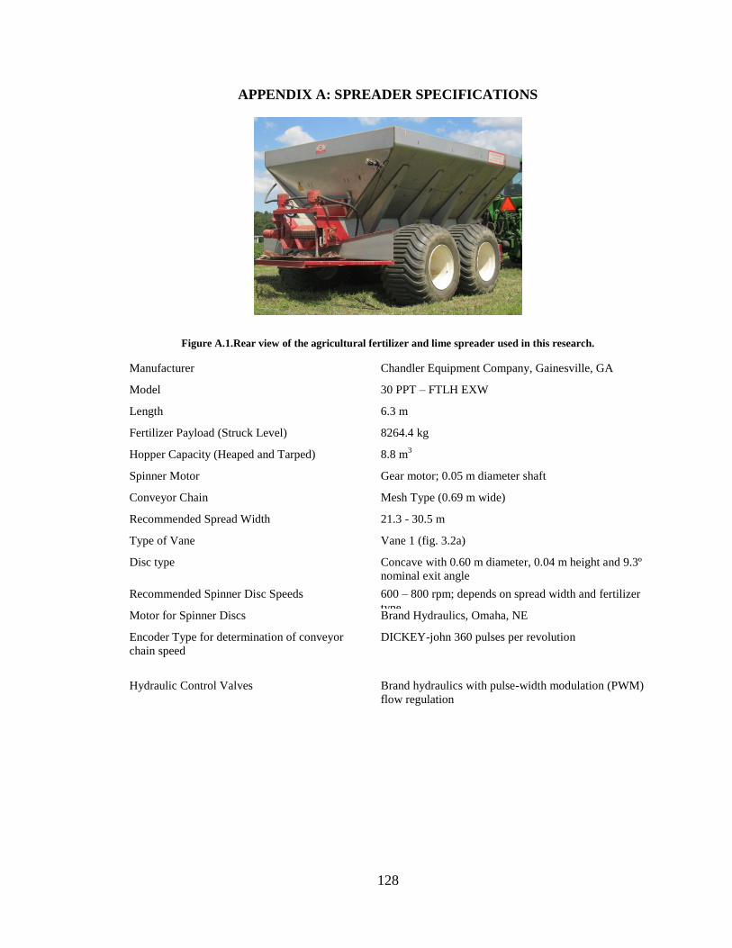
128
APPENDIX A: SPREADER SPECIFICATIONS
Figure A.1.Rear view of the agricultural fertilizer and lime spreader used in this research.
Manufacturer Chandler Equipment Company, Gainesville, GA
Model 30 PPT – FTLH EXW
Length 6.3 m
Fertilizer Payload (Struck Level) 8264.4 kg
Hopper Capacity (Heaped and Tarped) 8.8 m3
Spinner Motor Gear motor; 0.05 m diameter shaft
Conveyor Chain Mesh Type (0.69 m wide)
Recommended Spread Width 21.3 - 30.5 m
Type of Vane Vane 1 (fig. 3.2a)
Disc type Concave with 0.60 m diameter, 0.04 m height and 9.3º
nominal exit angle
Recommended Spinner Disc Speeds 600 – 800 rpm; depends on spread width and fertilizer
type Motor for Spinner Discs Brand Hydraulics, Omaha, NE
Encoder Type for determination of conveyor
chain speed
DICKEY-john 360 pulses per revolution
Hydraulic Control Valves Brand hydraulics with pulse-width modulation (PWM)
flow regulation

129
Figure A.2. Hydraulic circuit for the conveyor and spinner discs (Chandler Spreaders, 2013).
Part No. Description
A. 400-C-209 B P-2500 Tandem Pump 0.06 m X 0.06 m
B. 400-1-308 Relief valve- Nonadustable-2500 PSI
C. 400-1-313 Flow Control Valve with Built-in-Relief
D. Options063-0171-846063-0172-19435-02128 Control Valve Raven: 30 GPM PWM Fast Valve
Teejet: 30 GPM EXR-4
E. 400-R-106400-R-104 Parker-MB-18-Single Rawson Drive
Parker-MB-12-Twin Rawson Drive
F. 400-C-218B M-2500 2” Gear Spinner Motor
G. 300-1-208 Filter gauge
H. 300-FL-113A EXW-Filter
I. 400-1-317 Breather Cap

130
Figure A.3. Exploded view of spinner assembly (Chandler Spreaders, 2013).
Part No. Description
A. 400-C-218 B M-2500-0.05 m Gear Spinner Motor
B. 300-1-210 Spinner Shaft M25
300-1-211 Spinner Shaft-Stainless M25
C. 300-FL-112 4 Bolt Spinner Hub
300-FL-112A 4 Bolt Spinner Hub-Stainless
D. 300-FL-114063-0171-846063-0172-
19435-02128
0.01 m Hex Head Flange Nut
E. 300-EXW-103400-R-104 F/L EXW H/T Spinner Blades
F. 300-EXW-101 Spinner Disc
300-EXW-102 Spinner Disc-Stainless
G. 300-1-208 Lock Collar
H. 300-FL-113A .01X.03 m Hex Head Bolt
I. UCP-207-20 Pillow Block Bearing
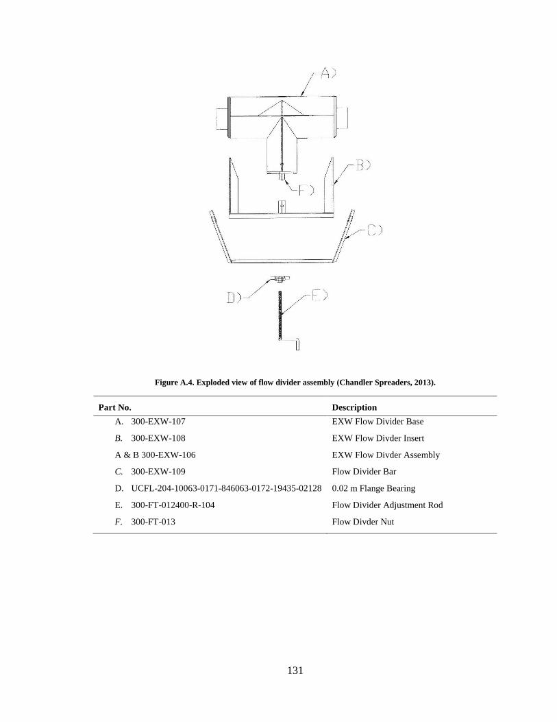
131
Figure A.4. Exploded view of flow divider assembly (Chandler Spreaders, 2013).
Part No. Description
A. 300-EXW-107 EXW Flow Divider Base
B. 300-EXW-108 EXW Flow Divder Insert
A & B 300-EXW-106 EXW Flow Divder Assembly
C. 300-EXW-109 Flow Divider Bar
D. UCFL-204-10063-0171-846063-0172-19435-02128 0.02 m Flange Bearing
E. 300-FT-012400-R-104 Flow Divider Adjustment Rod
F. 300-FT-013 Flow Divder Nut

132
Figure A.5. Conveyor Assembly (Chandler Spreaders, 2013).
Part No. Description
A. HWC-R-2434 Rear Roller Assembly
B. UCF-211-32 Flange Bearing
C. HWC-F-2434-EXW Front Roller Assembly-EXW
D. UCF-208-24063-0171-846063-0172-19435-02128 Flange Bearing
E. 300-FT-008400-R-104 Roller Adjustment Rod
F. 500-3-309 Connecting Pin 0.61 m
G. 500-3-304 Mest Type Chain-0.61 m (7.72 lg)
H. 100-R-1-01 Gear Case - Single
100-R-2-01 Gear Case – Twin
100-R-1-01A Gear Case – Single with Rate Sensor Port
100-R-2-01A Gear Case – Twin with Rate Sensor Port
I. 400-R-106 Hydraulic Motor – MB16 (Single Gear
Case) 400-R-104 Hydraulic Motor-MB16 (Twin Gear Case)
F. 300-EXW Encoder Mounting Bracket

133
Figure A.6. Electronically adjustable proportional pressure compensated flow controls (EFC). EFC12-10-12
(Left) and EFC12-15-12R22(Right)
Features
Weight 3.9 kg
Standard Port Size #12SAE (1-1/16-12)
Filtration 10-Micron
Pulse Frequency 90-115 Hz
Response Time 0.035” Standard dash pot (375 ms)
0.020” Dash pot (900 ms)
0.093” Dash pot (175 ms to 350 ms depending on flow
Spool Leakage 50 ml/min@1000 psi on EX port
Coil 12 VDC standard (24VDC)
9.6 ohms (48 ohms)
15 watts (15 watts)
1.0 amp max (0.5 amp max.)
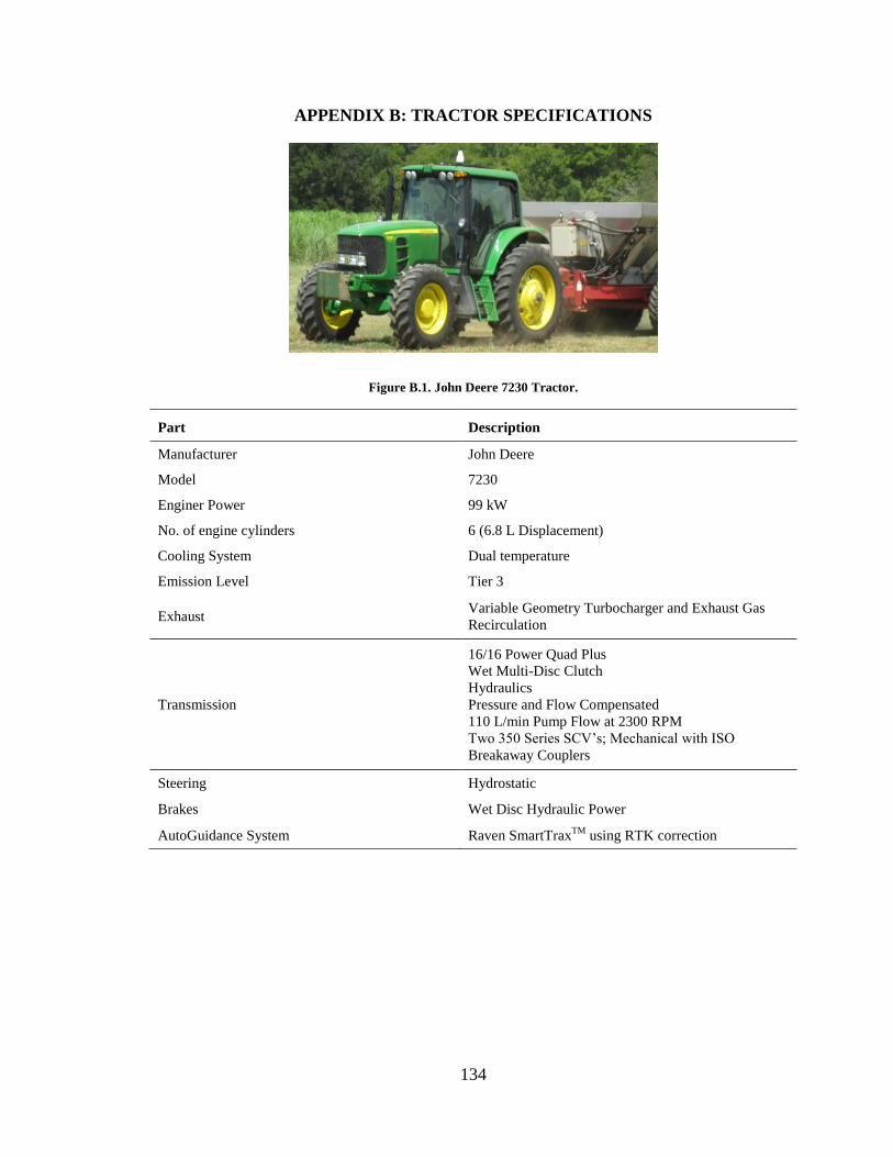
134
APPENDIX B: TRACTOR SPECIFICATIONS
Figure B.1. John Deere 7230 Tractor.
Part Description
Manufacturer John Deere
Model 7230
Enginer Power 99 kW
No. of engine cylinders 6 (6.8 L Displacement)
Cooling System Dual temperature
Emission Level Tier 3
Exhaust Variable Geometry Turbocharger and Exhaust Gas
Recirculation
Transmission
16/16 Power Quad Plus
Wet Multi-Disc Clutch
Hydraulics
Pressure and Flow Compensated
110 L/min Pump Flow at 2300 RPM
Two 350 Series SCV’s; Mechanical with ISO
Breakaway Couplers
Steering Hydrostatic
Brakes Wet Disc Hydraulic Power
AutoGuidance System Raven SmartTraxTM
using RTK correction

135
APPENDIX C: RAVEN ENVIZIO PRO SPECIFICATIONS
Figure C.1. RAVEN ENVIZIO PRO and switch pro displaying calibration settings for the spreader
Dimension 0.16 m diagonal measure
Processor 1.6 GHz 32 Bit
RAM Memory 1.0 GB
Internal Storage 2.0 GB
Operating System Microsoft Windows CE
Integrated Dual Frequency GPS Receiver
NMEA Output GGA, GGL, GSA, GSV,
RMC,
VTG and ZDA
Update Rate 1, 5 and 10 Hz (GSV at 0.2
Hz MAX)
Horizontal Position Accuracy (RMS)
Signal Point L1 1.5 m
Single Point L1/L2 1.2 m
SBAS 0.6 m
DGPS 0.4 m
RTK-2 1 cm+1 ppm
OMNISTAR VBS 0.6 m
OMNISTAR XP 0.2 m
OMNISTAR HP 0.1 m
USB Data Transfer Ports 2
CANBUS 2.0B COMPATIBLE SERIAL PORTS 2
RS232 SERIAL DATA PORTS 3 (GPS, CONSOLE,
AUXILIARY)
Min. Speed Output 0.80 km h-1
Power 24 W Typ.
Switched Output 12 [email protected]
Density 67.0
Rate Cal 400
Spreader Constant 359
Rate Bump 25

136
APPENDIX D: MASS OF POTASH COLLECTED BY ZONE FOR THE STATIONARY TESTS IN CHAPTER 3
Table D.1. Mass of potash collected in different zones of collection device for Vane 1.
Rep Rate
(kg ha-1) Disc Speed (rpm)
Collected Mass (g)
Total Mass Envizio (g) Mass Percentage by Zone (%)
Zone No.
1 2 3 4 5 6 7 1 2 3 4 5 6 7
1
448
600 799.1 1894.0 6898.0 6971.1 6987.1 2102.5 6099.7 31751 2.5 6.0 21.7 22.0 22.0 6.6 19.2
800 348.7 1479.6 6900.0 8108.4 6770.0 1746.8 14562.6 39916 0.9 3.7 17.3 20.3 17.0 4.4 36.5
700 223.5 1316.3 6865.0 8414.4 7010.2 1895.0 10109.4 35834 0.6 3.7 19.2 23.5 19.6 5.3 28.2
224
700 248.2 1608.8 6843.7 7995.3 6782.6 1916.4 9985.2 35380 0.7 4.5 19.3 22.6 19.2 5.4 28.2
800 285.1 1181.1 5954.2 6935.1 5933.7 1423.1 12760.7 34473 0.8 3.4 17.3 20.1 17.2 4.1 37.0
600 393.5 1722.7 7339.9 7558.3 7455.4 2115.4 6980.6 33566 1.2 5.1 21.9 22.5 22.2 6.3 20.8
2
448
700 240.0 1208.0 7351.4 8468.4 7553.9 1827.9 8277.0 34927 0.7 3.5 21.0 24.2 21.6 5.2 23.7
800 261.8 1110.4 6383.4 7591.5 6468.8 1486.7 12077.6 35380 0.7 3.1 18.0 21.5 18.3 4.2 34.1
600 284.4 1309.3 7687.5 9201.8 7915.7 2058.4 5562.3 34019 0.8 3.8 22.6 27.0 23.3 6.1 16.4
224
800 274.0 1023.9 6467.2 6976.3 6663.2 1541.0 11073.8 34019 0.8 3.0 19.0 20.5 19.6 4.5 32.6
600 215.4 1500.2 8163.5 8032.3 8297.6 2259.2 6912.0 35380 0.6 4.2 23.1 22.7 23.5 6.4 19.5
700 204.0 1336.4 7112.4 8056.2 7451.1 2014.8 8298.1 34473 0.6 3.9 20.6 23.4 21.6 5.8 24.1
3
224
600 190.0 1713.8 7652.3 7923.0 8005.2 2409.4 8393.7 36287 0.5 4.7 21.1 21.8 22.1 6.6 23.1
800 210.5 998.5 5953.7 6751.2 6169.1 1434.4 12502.0 34019 0.6 2.9 17.5 19.8 18.1 4.2 36.7
700 189.4 1160.1 7090.4 7380.8 7272.2 1747.1 8272.2 33112 0.6 3.5 21.4 22.3 22.0 5.3 25.0
448
800 318.4 976.3 6698.4 8158.0 6808.7 1526.0 10440.8 34927 0.9 2.8 19.2 23.4 19.5 4.4 29.9
600 221.8 1383.2 7691.7 7929.9 7958.5 2077.4 7664.1 34927 0.6 4.0 22.0 22.7 22.8 5.9 21.9
700 244.5 1221.8 7522.8 8038.0 7712.1 1917.8 7816.0 34473 0.7 3.5 21.8 23.3 22.4 5.6 22.7
Mean 0.8 3.9 20.2 22.4 20.7 5.4 26.6
SD 0.4 0.8 1.9 1.7 2.1 0.9 6.5
CV 0.5 0.2 0.1 0.1 0.1 0.2 0.2

137
Table D.2. Mass of potash collected in different zones of collection device for Vane 2.
Rep
Rate
(kg ha-1)
Disc Speed
(rpm)
Collected Mass (g)
Total Mass
Envizio (g)
Mass Percentage by Zone (%) Zone No.
1 2 3 4 5 6 7 1 2 3 4 5 6 7
1
224
700 283.2 1668.0 7990.3 10117.2 8541.8 1594.6 4731.6 34927 0.8 4.8 22.9 29.0 24.5 4.6 13.5
600 198.3 1714.9 8358.6 8672.1 8719.6 1611.5 5651.7 34927 0.6 4.9 23.9 24.8 25.0 4.6 16.2
800 221.1 1262.0 7686.6 9128.2 8079.2 1209.6 6432.7 34019 0.6 3.7 22.6 26.8 23.7 3.6 18.9
448
800 249.6 1263.6 7791.3 9700.5 8251.8 1207.3 6009.0 34473 0.7 3.7 22.6 28.1 23.9 3.5 17.4
600 218.0 1647.9 8443.6 8518.7 8789.3 1460.9 5394.5 34473 0.6 4.8 24.5 24.7 25.5 4.2 15.6
700 246.0 1455.6 8273.3 9958.6 8659.0 1366.5 4060.5 34019 0.7 4.3 24.3 29.3 25.5 4.0 11.9
2
448
600 168.1 1672.0 9294.9 9339.9 9711.6 1827.8 2912.3 34927 0.5 4.8 26.6 26.7 27.8 5.2 8.3
800 223.9 1344.8 7793.3 12524.0 8490.1 1304.0 3700.1 35380 0.6 3.8 22.0 35.4 24.0 3.7 10.5
700 262.9 1385.0 8181.1 10401.7 8983.2 1299.5 3959.6 34473 0.8 4.0 23.7 30.2 26.1 3.8 11.5
224
800 250.3 1010.2 8218.9 9074.1 8802.8 1157.4 5052.1 33566 0.7 3.0 24.5 27.0 26.2 3.4 15.1
700 237.1 1504.7 7929.8 9213.0 8404.6 1411.1 5319.1 34019 0.7 4.4 23.3 27.1 24.7 4.1 15.6
600 256.7 1755.9 8597.4 9536.2 9310.1 1638.6 3831.7 34927 0.7 5.0 24.6 27.3 26.7 4.7 11.0
3
448
800 278.6 1025.0 8595.2 10166.9 9109.4 1038.3 4713.2 34927 0.8 2.9 24.6 29.1 26.1 3.0 13.5
700 267.4 1158.6 8470.9 9433.8 9363.8 1348.1 5337.6 35380 0.8 3.3 23.9 26.7 26.5 3.8 15.1
600 225.3 1299.3 9227.3 9263.7 9591.6 1385.0 2573.6 33566 0.7 3.9 27.5 27.6 28.6 4.1 7.7
224
600 161.8 1374.8 9202.0 9155.9 9850.2 1475.8 3252.5 34473 0.5 4.0 26.7 26.6 28.6 4.3 9.4
800 421.3 876.1 7934.9 10467.0 8724.1 924.3 4671.7 34019 1.2 2.6 23.3 30.8 25.6 2.7 13.7
700 260.0 1014.6 8899.5 10393.8 9341.4 1124.8 3438.9 34473 0.8 2.9 25.8 30.2 27.1 3.3 10.0
Mean 0.7 3.9 24.3 28.2 25.9 3.9 13.1
SD 0.2 0.8 1.5 2.5 1.5 0.6 3.2
CV 0.2 0.2 0.1 0.1 0.1 0.2 0.2

138
Table D.3. Mass of potash collected in different zones of collection device for Vane 3.
Rep Rate
(kg ha-1) Disc Speed (rpm)
Collected Mass (g)
Total Mass Envizio (g) Mass Percentage by Zone (%)
Zone No.
1 2 3 4 5 6 7 1 2 3 4 5 6 7
1
224
800 142.3 422.6 8397.7 8562.6 8938.3 502.2 7053.7 34019 0.4 1.2 24.7 25.2 26.3 1.5 20.7
600 136.5 901.7 9972.1 7895.4 10859 891.8 2909.2 33566 0.4 2.7 29.7 23.5 32.4 2.7 8.7
700 119.8 795.8 9952.2 8590.9 10589 833.6 5406.6 36287 0.3 2.2 27.4 23.7 29.2 2.3 14.9
448
700 113 985.6 9636.9 8343.1 10470 954.9 4876.8 35380 0.3 2.8 27.2 23.6 29.6 2.7 13.8
800 189.5 946.8 8381.1 9874.8 8838.7 795.8 9075.06 38102 0.5 2.5 22.0 25.9 23.2 2.1 23.8
600 173.9 1554.5 9896.3 8700.3 10546 1535 2067.4 34473 0.5 4.5 28.7 25.2 30.6 4.5 6.0
2
224
600 195.9 1541 9759.1 8656.7 10610 1468.2 3602.5 35834 0.5 4.3 27.2 24.2 29.6 4.1 10.1
700 142.3 986.5 9180.7 8067.3 9972.7 893.7 6137.0 35380 0.4 2.8 25.9 22.8 28.2 2.5 17.3
800 339.6 537.1 8632 9061.9 8952.8 589.8 5906.2 34019 1.0 1.6 25.4 26.6 26.3 1.7 17.4
448
800 236.5 706.6 7656.6 8349.7 8529.8 611.5 8835.9 34927 0.7 2.0 21.9 23.9 24.4 1.8 25.3
700 190.3 1104.4 10072 9101 9627.6 1014.6 4270.0 35380 0.5 3.1 28.5 25.7 27.2 2.9 12.1
600 175 1177.4 10073 8417.8 10730 963.4 2482.4 34019 0.5 3.5 29.6 24.7 31.5 2.8 7.3
3
448
800 155.8 900.1 8046.9 8379.6 8530.1 828 8086.1 34927 0.4 2.6 23.0 24.0 24.4 2.4 23.2
600 158.8 1425 10397 8222.7 11158 1222.4 1436.4 34019 0.5 4.2 30.6 24.2 32.8 3.6 4.2
700 140.3 981.7 9470.8 7923.2 9753.3 912.1 4384.4 33566 0.4 2.9 28.2 23.6 29.1 2.7 13.1
224
700 143.9 1080.4 10120 8295.9 10669 958.8 4112.2 35380 0.4 3.1 28.6 23.4 30.2 2.7 11.6
800 214.5 763.5 8668.6 9361.3 9212.9 722.5 4622.5 33566 0.6 2.3 25.8 27.9 27.4 2.2 13.8
600 117.7 1560.2 9568 8132.9 10460 1601.7 4393.2 35834 0.3 4.4 26.7 22.7 29.2 4.5 12.3
Mean 0.5 2.9 26.7 24.5 28.4 2.7 14.2
SD 0.2 0.9 2.6 1.4 2.7 0.9 6.1
CV 0.3 0.3 0.1 0.1 0.1 0.3 0.4

139
Table D.4. Mass of potash collected in different zones of collection device for Vane 4.
Rep Rate
(kg ha-1) Disc Speed rpm
Collected Mass (g)
Total Mass Envizio (g) Mass Percentage by Zone (%)
Zone No.
1 2 3 4 5 6 7 1 2 3 4 5 6 7
1
448
700 192.7 1202.7 10177.3 7939.6 10603.0 1024.2 2879.9 34019 0.6 3.5 29.9 23.3 31.2 3.0 8.5
800 485.9 1012.5 9272.8 9556.0 10166.1 887.9 3091.8 34473 1.4 2.9 26.9 27.7 29.5 2.6 9.0
600 107.6 1930.2 10349.2 7856.4 11000.9 1762.6 3280.5 36287 0.3 5.3 28.5 21.7 30.3 4.9 9.0
224
600 174.9 1327.7 10428.3 8513.1 11526.8 1246.0 349.0 33566 0.5 4.0 31.1 25.4 34.3 3.7 1.0
700 159.5 1150.0 10375.7 8740.7 10960.5 980.0 1653.0 34019 0.5 3.4 30.5 25.7 32.2 2.9 4.9
800 144.2 1477.0 9545.2 7571.8 9907.8 1220.2 4606.8 34473 0.4 4.3 27.7 22.0 28.7 3.5 13.4
2
224
600 155.2 1393.9 10578.6 8629.4 11389.3 1192.2 1134.4 34473 0.5 4.0 30.7 25.0 33.0 3.5 3.3
800 145.3 1596.9 9732.4 8736.2 10634.6 1329.6 2751.6 34927 0.4 4.6 27.9 25.0 30.4 3.8 7.9
700 199.5 1666.3 9758.5 8378.6 10593.4 1452.9 1516.6 33566 0.6 5.0 29.1 25.0 31.6 4.3 4.5
448
800 169.6 1284.9 9330.4 8929.2 9751.4 1132.2 3875.3 34473 0.5 3.7 27.1 25.9 28.3 3.3 11.2
700 139.7 1695.9 9970.6 8719.0 10679.4 1516.4 2659.2 35380 0.4 4.8 28.2 24.6 30.2 4.3 7.5
600 144.3 1498.7 10440.1 7622.5 11398.8 1300.9 2521.3 34927 0.4 4.3 29.9 21.8 32.6 3.7 7.2
3
448
800 126.0 1615.0 10870.0 7495.6 11810.3 1425.9 1130.2 34473 0.4 4.7 31.5 21.7 34.3 4.1 3.3
600 119.4 1626.9 10895.0 7498.6 11883.9 1400.6 595.0 34019 0.4 4.8 32.0 22.0 34.9 4.1 1.7
700 112.9 1702.2 10452.2 8436.7 11322.3 1563.3 1337.0 34927 0.3 4.9 29.9 24.2 32.4 4.5 3.8
224
600 114.4 1911.0 10295.7 7746.7 11320.9 1794.0 1743.9 34927 0.3 5.5 29.5 22.2 32.4 5.1 5.0
700 157.7 1676.6 9789.0 8250.5 10688.3 1581.5 1875.8 34019 0.5 4.9 28.8 24.3 31.4 4.6 5.5
800 187.6 1386.1 9339.6 8107.9 10283.7 1207.6 3960.5 34473 0.5 4.0 27.1 23.5 29.8 3.5 11.5
Mean 0.5 4.4 29.2 23.9 31.5 3.9 6.6
SD 0.2 0.7 1.6 1.8 1.9 0.7 3.5
CV 0.5 0.2 0.1 0.1 0.1 0.2 0.5

140
APPENDIX E: SUMMARIZED DATA TABLES AND FIGURES ALONG WITH
INCLUDED STATISTICS.
Table E.1. Overall mean mass material distribution (%) for all four vane shapes at feed rate of 448
kg ha-1
in different zones of the collection device at three spinner disc-speeds of 600, 700 and 800
rpm.
Vane Disc Speed
(rpm)
Zone No.
2 3 4 5 6
1
600
5.7a
27.8c
30.1a
28.6b
7.8a
2 5.0b
29.5b
29.7ab
30.7b
5.1b
3 4.3a
31.6a
26.4bc
33.8a
3.9b
4 5.1a
32.2a
23.3c
34.8a
4.5b
1
700
4.8a 27.8
b 31.8
a 28.4
c 7.2
a
2 4.5ab
27.8b 33.2
a 30.1
bc 4.5
b
3 3.4b 32.3
a 28.1
b 33.0
ab 3.2
c
4 4.7a 31.5
a 25.9
b 33.6
a 4.2
bc
1
800
4.9a 27.7
b 33.0
ab 27.8
c 6.6
a
2 4.1a 27.0
b 36.1
a 28.9
bc 4.0
b
3 3.1a 29.6
ab 32.7
ab 31.8
ab 2.7
b
4 4.1c 31.2
a 27.5
b 33.6
a 3.6
b
Means denoted by the same letter are not significantly different (level of confidence α = 95%) within a column for a
particular spinner-disc speed.
Table E.2. Overall mean mass material distribution (%) within in Zones 2 and 6 at feed rate of 224
kg ha-1
, along with p-values comparing data within a specific treatment.
Vane Disc Speed
(rpm)
Zone No.
p-value 2 6
1
600
5.7 7.8 0.2474
2 5.0 5.1 1.0000
3 4.3 3.9 0.6719
4 5.1 4.5 0.4227
1
700
4.8 7.2 0.1367
2 4.5 4.5 0.8335
3 3.4 3.2 0.2414
4 4.7 4.2 0.4164
1
800
4.9 6.6 0.1413
2 4.1 4.0 0.8335
3 3.1 2.7 0.3187
4 4.1 3.6 0.6807

141
Table E.3. Overall mean mass material distribution (%) within Zones 3 and 5 at feed rate of 448 kg
ha-1
along with p-values comparing data within a specific treatment.
Vane Disc Speed
(rpm)
Zone No.
p-value 3 5
1
600
27.8 28.6 0.4164
2 29.5 30.7 0.1228
3 31.6 33.8 0.1367
4 32.2 34.8 0.1413
1
700
27.8 28.4 0.4227
2 27.8 30.1 0.1413
3 32.3 33.0 0.6764
4 31.5 33.6 0.2474
1
800
27.7 27.8 0.6764
2 27.0 28.9 0.4227
3 29.6 31.8 0.1413
4 31.2 33.6 0.2474
Table E.4. Average percent material captured by zones when considering only Zones 2 through 6 or
zones where controlled distribution occurred at feed rate of 224 kg ha-1
.
Vane Zone Speed Tukey Grouping
CHAN 5 600 A
TAP 5 700 A B
TAP 5 600 A B C
ORGM 4 800 A B C D
CHAN 5 700 A B C D E
CHAN 5 800 A B C D E
ORGM 4 700 A B C D E F
TAP 5 800 A B C D E F G
TAP 4 800 A B C D E F G
TAP 3 700 A B C D E F G H
ORG 4 800 B C D E F G H I
CHAN 3 600 B C D E F G H I J
TAP 3 600 C D E F G H I J K
CHAN 3 700 D E F G H I J K L
CHAN 3 800 D E F G H I J K L
ORG 4 700 E F G H I J K L M
TAP 3 800 E F G H I J K L M N
ORGM 5 600 F G H I J K L M N O
ORGM 5 800 G H I J K L M N O P
ORGM 4 600 G H I J K L M N O P Q
ORGM 5 700 H I J K L M N O P Q
ORG 5 600 I J K L M N O P Q R
ORGM 3 600 J K L M N O P Q R
ORG 5 800 K L M N O P Q R
ORG 4 600 K L M N O P Q R
ORG 5 700 L M N O P Q R

142
ORGM 3 800 M N O P Q R
ORG 3 600 M N O P Q R
ORG 3 800 N O P Q R
ORGM 3 700 O P Q R S
ORG 3 700 P Q R S
TAP 4 700 Q R S
CHAN 4 800 R S
CHAN 4 700 R S
TAP 4 600 R S
CHAN 4 600 S
ORG 6 600 T
ORG 6 700 T U
ORG 6 800 T U V
ORG 2 600 T U V W
ORG 2 700 U V W X
ORGM 2 600 U V W X
ORGM 6 600 U V W X
ORG 2 800 U V W X Y
CHAN 2 800 U V W X Y
Z
ORGM 2 700 U V W X Y
Z
CHAN 2 700 U V W X Y
Z
CHAN 2 600 V W X Y
Z
ORGM 6 700 V W X Y
Z
CHAN 6 600 V W X Y
Z
TAP 2 600 V W X Y
Z
TAP 6 600 V W X Y
Z
CHAN 6 700 V W X Y
Z
CHAN 6 800 V W X Y
Z
ORGM 6 800 W X Y
Z
ORGM 2 800 W X Y
Z
TAP 2 700 X Y
Z
TAP 6 700 X Y
Z

143
TAP 6 800 Y
Z
TAP 2 800
Z
Table E.5. Average percent material captured by zone when considering only Zones 2 through 6 or
zones where controlled distribution occurred at feed rate of 224 kg ha-1
.
Vane
Disc
Speed
(rpm)
Zone No.
2 3 4 5 6
Average Mass (%)
1
600
6.0tuvw
28.2mnopqr
28.6klmnopqr
28.9ijklmnopqr
8.3t
2 5.3uvwx
28.8jklmnopqr
30.1ghijklmnopq
30.6fghijklmno
5.2uvwx
3 4.3vwxyz
31.2cdefghijk
26.3rs
34.0abc
4.2vwxyz
4 4.7vwxyz
31.5bcdefghi
25.1s
34.5a
4.3vwxyz
1
700
5.4uvwx
27.8opqrs
30.9efghijklm
28.4lmnopqr
7.5tu
2 4.7uvwxyz
27.8opqrs
33.3abcdef
29.5hijklmnopq
4.6vwxyz
3 3.1xyz
32.2abcdefgh
27.4qrs
34.3ab
3.0xyz
4 4.7vwxyz
31.2defghijkl
26.4rs
33.6
4.2vwxyz
1
800
4.9uvwxy
28.1nopqr
31.6bcdefghi
28.7klmnopqr
6.7tuv
2 3.7wxyz
28.2mnopqr
33.9abcd
30.3ghijklmnop
3.9wxyz
3 2.1z
30.8efghijklmn
32.4abcdefg
32.5abcdefg
2.2yz
4 4.8uvwxyz
31.1defghijkl
26.5rs
33.5abcde
4.1vwxyz
Means denoted by the same letter are not significantly different (level of confidence α = 95%).
Table E.6. Impact of increase in spinner disc speed on maximum transverse distance by Vane.
Vane
------------------- Disc Speed (rpm) --------------------
600 700 800
1 13.4 15.3 16.4
2 13.3 14.9 16.4
3 13.4 14.1 16.4
4 14.5 14.9 16.4

144
Table E.7. Summary of the overlap pattern analyses at effective spread widths of 18.3 and 21.3 m for
the four vane designs along with skewing.
18.3-m Spread
Width
21.3-m Spread
Width
Van
e
Target
Rate
(kg ha-1
)
Disc
Speed
(rpm)
Skewing
(%Left/%Right
)
Mean
Rate
(kg ha-1
)
CV
(%)
Mean
Rate
(kg ha-1
)
CV
(%)
1
224
600 46.7/53.3 263.6 31.4 211.8 45.1
700 47.0/53.0 262.5 42.1 210.3 29.9
800 43.3/56.8 252.0 40.9 206.6 40.0
448
600 46.6/53.4 494.1 30.5 397.3 44.6
700 45.0/55.0 475.3 45.6 378.5 35.6
800 46.7/53.3 394.8 41.2 323.1 41.4
2
224
600 48.5/51.5 276.5 26.0 222.5 42.3
700 46.2/53.8 304.5 47.1 241.1 30.6
800 44.5/55.5 257.0 38.4 210.2 31.7
448
600 47.1/52.9 539.7 33.8 431.9 41.2
700 47.0/53.0 492.9 41.3 387.6 26.4
800 45.9/54.1 479.6 39.7 391.4 34.5
3
224
600 47.5/52.5 292.6 35.8 236.4 51.3
700 44.7/55.3 306.0 43.1 243.9 28.5
800 45.1/54.9 284.3 43.0 228.7 28.1
448
600 49.2/50.8 544.4 36.5 436.2 50.2
700 45.1/54.9 559.6 52.5 445.0 36.3
800 45.9/54.9 521.6 45.6 4109.7 31.4
4
224
600 49.7/50.3 312.4 40.3 250.2 48.0
700 47.9/52.1 320.7 46.7 255.0 29.4
800 44.8/55.2 311.3 46.8 254.9 37.7
448
600 48.3/51.7 583.9 42.6 468.4 51.2
700 46.1/53.9 569.8 5308 453.5 35.7
800 45.5/54.5 513.3 52.4 416.0 42.0

145
Figure E1. Impact of increase in spinner-disc speed on ricocheting (± 1 SD) for all the four vane shapes at a feed
rate of 224 kg ha-1. Means denoted by the same letters are not significantly different (α = 95%).
(a) Vane 1
(b) Vane 2
bc
b
a
de dcd
def
cd
cd
f ef
de
0.0
10.0
20.0
30.0
40.0
50.0
600 700 800
Ric
oc
he
tin
g (
%)
Spinner Disc Speed (rpm)
Vane-1 Vane-2 Vane-3 Vane-4
0.0
1.1
2.2
-18.5 -13.9 -9.3 -4.6 0.0 4.6 9.2 13.8 18.5
Sta
nd
ard
ize
d
Dis
trib
uti
on
Patt
ern
Tranverse Location (m)
224 kg/ha600 RPM700 RPM800 RPM
0.0
1.1
2.2
-18.5 -13.9 -9.3 -4.6 0.0 4.6 9.2 13.8 18.5
Sta
nd
ard
ize
d
Dis
trib
uti
on
Patt
ern
Tranverse Location (m)
448 kg/ha600 RPM
700 RPM
800 RPM
0.0
1.1
2.2
-18.5 -13.9 -9.3 -4.6 0.0 4.6 9.2 13.8 18.5
Sta
nd
ard
ized
D
istr
ibu
tio
n P
att
ern
Tranverse Location (m)
224 kg/ha600 RPM
700 RPM
800 RPM
0.0
1.1
2.2
-18.5 -13.9 -9.3 -4.6 0.0 4.6 9.2 13.8 18.5
Sta
nd
ard
ize
d D
istr
ibu
tio
n
Patt
ern
Tranverse Location (m)
448 kg/ha600 RPM700 RPM800 RPM

146
(c) Vane 3
(d) Vane 4
Figure E2. Standardized distribution patterns at 224 kg/h and 448 kg/ha for each vane design. Each curve
within the plot represents the mean of three replications. Transverse location represents pan position across the
spread width; 0 represents the centreline of the spreader with negative values the left side of the spreader and
positive values on the right.
0.0
1.1
2.2
-18.5 -13.9 -9.3 -4.6 0.0 4.6 9.2 13.8 18.5
Sta
nd
ard
ized
D
istr
ibu
tio
n P
att
ern
Tranverse Location (m)
224 kg/ha600 RPM700 RPM800 RPM
0.0
1.1
2.2
-18.5 -13.9 -9.3 -4.6 0.0 4.6 9.2 13.8 18.5
Sta
nd
ard
ize
d
Dis
trib
uti
on
Patt
ern
Tranverse Location (m)
448 kg/ha600 RPM700 RPM800 RPM
0.0
1.1
2.2
-18.5 -13.9 -9.3 -4.6 0.0 4.6 9.2 13.8 18.5
Sta
nd
ard
ized
D
istr
ibu
tio
n P
att
ern
Tranverse Location (m)
224 kg/ha600 RPM700 RPM800 RPM
0.0
1.1
2.2
-18.5 -13.9 -9.3 -4.6 0.0 4.6 9.2 13.8 18.5S
tan
da
rdiz
ed
D
istr
ibu
tio
n P
att
ern
Tranverse Location (m)
448 kg/ha600 RPM700 RPM800 RPM

147
Table E.8. Impact of increase in spinner disc speed on the level of segregation for P2O5 and K2O at all
transverse pan locations across the swath.
Pan Location
(m)
P2O5% K2O%
600 700 800 600 700 800
-18.3 0.0ci
46.0a
46.0a
0.0ci
0.0ci
0.0ci
-17.5 0.0ci
45.1b
43.0f
0.0ci
0.0ci
4.0cd
-16.8 46.0a
43.7e
40.7j
0.0ci
3.0cf
7.0by
-16.0 46.0a
40.7j
36.8q
0.0ci
6.9bz
12.0bp
-15.2 46.0a
37.1p
33.8x
0.0ci
11.7br
16.0bh
-14.5 40.9i
35.7t
32.2ac
6.8ca
14.0bl
18.0bc
-13.7 37.7o
32.7ab
30.6ak
10.8bt
15.2bj
20.0aw
-13.0 35.8s
31.9ad
29.9an
13.3bn
17.4bd
21.0as
-12.2 34.3w
30.8ai
29.2ar
15.3bi
18.1bb
22.0ap
-11.4 31.6af
29.5ap
27.6az
18.8ba
21.0as
24.0ai
-10.7 31.3ah
28.4aw
26.0bk
19.2ay
22.3am
26.0w
-9.9 30.1am
26.5bg
24.6bv
20.8at
25.5z
28.0l
-9.1 30.2al
25.3bq
24.3bx
21.5ar
27.1q
28.3j
-8.4 28.0ay
24.8bu
23.9ca
23.4aj
27.6n
28.8g
-7.6 25.8bm
24.4bw
24.2by
26.3u
28.2k
28.5i
-6.9 25.2br
24.2by
23.9ca
27.1q
28.5i
28.8g
-6.1 25.1bs
23.9ca
23.7cc
27.3p
28.8g
29.1f
-5.3 24.4bw
24.2by
24.9bt
28.2k
28.5i
27.5o
-4.6 23.5cd
26.7bf
26.2bi
29.4d
24.8ad
25.9x
-3.8 23.3ce
28.0ay
25.7bn
29.7c
24.3ag
26.5t
-3.0 25.9bl
28.6au
26.2bi
26.3u
22.8al
25.8y
-2.3 26.7bf
28.5av
27.5ba
25.2aa
22.8al
24.1ah
0.0 29.1as
29.4aq
29.0at
22.0ap
21.6aq
22.2an
2.3 27.5ba
27.1bc
27.4bb
24.4af
24.6ae
24.4af
3.0 25.6bo
26.1bj
26.9bd
26.6s
26.0w
24.9ac
3.8 26.0bk
25.9bl
26.4bh
26.1v
26.3u
25.5z
4.6 24.6bv
24.1bz
24.8bu
27.9m
28.0l
27.6n
5.3 24.4bw
23.7cc
24.6bv
28.2k
29.2e
27.9m
6.1 23.8cb
23.0cg
24.4bw
28.6h
30.0b
28.2k
6.9 23.9ca
22.8ch
24.2by
28.8g
30.3a
28.5i
7.6 24.3bx
23.2cf
24.4bw
28.3j
29.7c
28.3j
8.4 24.6bv
27.1bc
24.6bv
28.0l
24.6ae
27.9m
9.1 29.1as
29.8ao
25.5bp
22.1ao
20.6au
26.7r
9.9 31.5ag
30.6ak
25.5bp
18.9az
20.1av
26.7r
10.7 33.5y
32.2ad
26.8be
16.2bg
18.0bc
25.1ab
11.4 34.9v
33.4z
28.3ax
14.5bk
16.5bf
23.1ak
12.2 37.8m
36.4r
29.4aq
10.7bu
12.8bo
21.5ar
13.0 40.2l
37.4p
30.7aj
7.7bw
11.8bq
19.9ax
13.7 40.3k
40.3k
33.1aa
6.2cb
7.2bx
16.9be
14.5 42.0g
44.6c
35.6u
3.8ce
1.8ch
13.7bm
15.2 46.0a
46.0a
37.4p
0.0ci
0.0ci
11.2bs
16.0 46.0a
0.0ci
39.3m
0.0ci
0.0ci
8.7bv
16.8 46.0a
0.0ci
41.9h
0.0ci
0.0ci
5.3cc
17.5 0.0ci
0.0ci
44.2d
0.0ci
0.0ci
2.5cg
18.3 0.0ci
0.0ci
46.0a
0.0ci
0.0ci
0.0ci
Means that do not share a letter are significantly different for P2O5 and K2O separately.

148
Table E.9. The impact of increase in feed rate on level of segregation represented by p-values on
nutrient concentration distribution for P2O5 and K2O at all transverse pan locations across the
swath.
Pan
Location
(m)
P2O5 (%) K2O (%)
224 kg ha-
1 448 kg ha
-
1
p-values 224 kg ha-
1
448 kg ha-
1
p-values
-18.3 30.7 29.8 0.1765 0.0 0.0 0.0500 -17.5 29.4 30.5 0.9161 1.3 1.2 0.1236 -16.8 28.9 29.4 0.0742 3.3 2.1 0.1595 -16.0 41.2 42.7 0.4019 6.3 6.8 0.9325
-15.2 39.0 39.3 0.8843 9.2 9.7 0.8633 -14.5 36.2 37.3 0.6776 12.9 12.7 0.6253 -13.7 33.7 36.3 0.3431 15.3 14.4 0.4503 -13.0 32.5 35.1 0.2789 17.2 16.1 0.3344 -12.2 31.4 34.4 0.2244 18.5 18.0 0.3595 -11.4 29.6 31.6 0.2883 21.3 21.2 0.3051 -10.7 28.6 29.5 0.5265 22.5 24.3 0.7315 -9.9 27.0 28.1 0.3348 24.8 26.8 0.6236 -9.1 26.6 25.5 0.2717 25.6 29.6 0.3335 -8.4 25.6 24.6 0.1701 26.6 30.9 0.1606 -7.6 24.8 24.3 0.0559 27.7 31.6 0.0530 -6.9 24.4 24.4 0.9110 28.1 31.3 0.8630 -6.1 24.2 25.2 0.5100 28.4 30.2 0.0530 -5.3 24.5 25.4 0.0578 28.1 29.9 0.0542 -4.6 25.5 26.8 0.2763 26.7 28.0 0.0504 -3.8 25.7 27.7 0.4587 26.8 26.9 0.0532 -3.0 26.9 28.5 0.7893 24.9 25.6 0.0522 -2.3 27.6 28.8 0.4571 24.0 25.1 0.0512 0.0 29.2 29.0 0.5677 21.9 23.8 0.0514 2.3 27.3 28.1 0.5789 24.4 26.0 0.0603 3.0 26.2 26.7 0.1688 25.9 28.0 0.2004 3.8 26.1 25.7 0.0555 26.0 29.4 0.0725 4.6 24.5 25.1 0.5487 27.8 30.4 0.0730 5.3 24.2 24.6 0.1033 28.4 31.2 0.1237 6.1 23.7 24.2 0.0701 28.9 31.6 0.1462 6.9 23.6 23.9 0.2466 29.2 32.0 0.2401 7.6 24.0 24.3 0.1436 28.7 31.6 0.1557 8.4 25.4 25.8 0.4523 26.8 29.3 0.4334 9.1 28.1 28.0 0.8561 23.1 26.1 0.7431 9.9 29.2 29.1 0.9241 21.9 24.5 0.9415 10.7 30.8 32.1 0.3637 19.8 21.2 0.6692 11.4 32.2 34.6 0.1557 18.0 16.9 0.1496 12.2 34.5 37.6 0.1542 15.0 12.6 0.1446 13.0 36.1 38.2 0.3239 13.1 11.4 0.2599 13.7 37.9 40.1 0.2783 10.1 8.9 0.3780 14.5 40.7 42.9 0.1830 6.4 5.5 0.2733 15.2 43.1 29.6 0.0920 3.7 3.2 0.2669 16.0 28.4 30.7 0.8342 2.9 2.5 0.0628 16.8 29.3 15.3 0.2070 1.8 1.2 0.0628 17.5 14.7 0.0 0.0620 0.8 0.7 0.0628 18.3 15.3 0.0 0.0628 0.0 0.0 0.0500

149
APPENDIX F: SAS PROGRAM CODE FOR ZONE ANALYSIS IN CHAPTER 3
F.1. Determination of behavior differences for mass collected in different zones of
collection device for individual vanes
Data fertilizer;
Input Vane$ Rep Rate Speed Z1 Z2 Z3 Z4 Z5 Z6 Z7;
DATALINES;
ORGM 1 200 700 0.8 4.8 22.9 29.0 24.5 4.6 13.5
ORGM 1 200 600 0.6 4.9 23.9 24.8 25.0 4.6 16.2
ORGM 1 200 800 0.6 3.7 22.6 26.8 23.7 3.6 18.9
ORGM 1 400 800 0.7 3.7 22.6 28.1 23.9 3.5 17.4
ORGM 1 400 600 0.6 4.8 24.5 24.7 25.5 4.2 15.6
ORGM 1 400 700 0.7 4.3 24.3 29.3 25.5 4.0 11.9
ORGM 2 400 600 0.5 4.8 26.6 26.7 27.8 5.2 8.3
ORGM 2 400 800 0.6 3.8 22.0 35.4 24.0 3.7 10.5
ORGM 2 400 700 0.8 4.0 23.7 30.2 26.1 3.8 11.5
ORGM 2 200 800 0.7 3.0 24.5 27.0 26.2 3.4 15.1
ORGM 2 200 700 0.7 4.4 23.3 27.1 24.7 4.1 15.6
ORGM 2 200 600 0.7 5.0 24.6 27.3 26.7 4.7 11.0
ORGM 3 400 800 0.8 2.9 24.6 29.1 26.1 3.0 13.5
ORGM 3 400 700 0.8 3.3 23.9 26.7 26.5 3.8 15.1
ORGM 3 400 600 0.7 3.9 27.5 27.6 28.6 4.1 7.7
ORGM 3 200 600 0.5 4.0 26.7 26.6 28.6 4.3 9.4
ORGM 3 200 800 1.2 2.6 23.3 30.8 25.6 2.7 13.7
ORGM 3 200 700 0.8 2.9 25.8 30.2 27.1 3.3 10.0
ORG 1 400 600 2.5 6.0 21.7 22.0 22.0 6.6 19.2
ORG 1 400 800 0.9 3.7 17.3 20.3 17.0 4.4 36.5
ORG 1 400 700 0.6 3.7 19.2 23.5 19.6 5.3 28.2
ORG 1 200 700 0.7 4.5 19.3 22.6 19.2 5.4 28.2
ORG 1 200 800 0.8 3.4 17.3 20.1 17.2 4.1 37.0
ORG 1 200 600 1.2 5.1 21.9 22.5 22.2 6.3 20.8
ORG 2 400 700 0.7 3.5 21.0 24.2 21.6 5.2 23.7
ORG 2 400 800 0.7 3.1 18.0 21.5 18.3 4.2 34.1
ORG 2 400 600 0.8 3.8 22.6 27.0 23.3 6.1 16.4
ORG 2 200 800 0.8 3.0 19.0 20.5 19.6 4.5 32.6
ORG 2 200 600 0.6 4.2 23.1 22.7 23.5 6.4 19.5
ORG 2 200 700 0.6 3.9 20.6 23.4 21.6 5.8 24.1
ORG 3 200 600 0.5 4.7 21.1 21.8 22.1 6.6 23.1
ORG 3 200 800 0.6 2.9 17.5 19.8 18.1 4.2 36.7
ORG 3 200 700 0.6 3.5 21.4 22.3 22.0 5.3 25.0
ORG 3 400 800 0.9 2.8 19.2 23.4 19.5 4.4 29.9
ORG 3 400 600 0.6 4.0 22.0 22.7 22.8 5.9 21.9
ORG 3 400 700 0.7 3.5 21.8 23.3 22.4 5.6 22.7
CHAN 1 400 700 0.6 3.5 29.9 23.3 31.2 3.0 8.5
CHAN 1 400 800 1.4 2.9 26.9 27.7 29.5 2.6 9.0
CHAN 1 400 600 0.3 5.3 28.5 21.7 30.3 4.9 9.0

150
CHAN 1 200 600 0.5 4.0 31.1 25.4 34.3 3.7 1.0
CHAN 1 200 700 0.5 3.4 30.5 25.7 32.2 2.9 4.9
CHAN 1 200 800 0.4 4.3 27.7 22.0 28.7 3.5 13.4
CHAN 2 200 600 0.5 4.0 30.7 25.0 33.0 3.5 3.3
CHAN 2 200 800 0.4 4.6 27.9 25.0 30.4 3.8 7.9
CHAN 2 200 700 0.6 5.0 29.1 25.0 31.6 4.3 4.5
CHAN 2 400 800 0.5 3.7 27.1 25.9 28.3 3.3 11.2
CHAN 2 400 700 0.4 4.8 28.2 24.6 30.2 4.3 7.5
CHAN 2 400 600 0.4 4.3 29.9 21.8 32.6 3.7 7.2
CHAN 3 400 800 0.4 4.7 31.5 21.7 34.3 4.1 3.3
CHAN 3 400 600 0.4 4.8 32.0 22.0 34.9 4.1 1.7
CHAN 3 400 700 0.3 4.9 29.9 24.2 32.4 4.5 3.8
CHAN 3 200 600 0.3 5.5 29.5 22.2 32.4 5.1 5.0
CHAN 3 200 700 0.5 4.9 28.8 24.3 31.4 4.6 5.5
CHAN 3 200 800 0.5 4.0 27.1 23.5 29.8 3.5 11.5
TAP 1 200 800 0.4 1.2 24.7 25.2 26.3 1.5 20.7
TAP 1 200 600 0.4 2.7 29.7 23.5 32.4 2.7 8.7
TAP 1 200 700 0.3 2.2 27.4 23.7 29.2 2.3 14.9
TAP 1 400 700 0.3 2.8 27.2 23.6 29.6 2.7 13.8
TAP 1 400 800 0.5 2.5 22.0 25.9 23.2 2.1 23.8
TAP 1 400 600 0.5 4.5 28.7 25.2 30.6 4.5 6.0
TAP 2 200 600 0.5 4.3 27.2 24.2 29.6 4.1 10.1
TAP 2 200 700 0.4 2.8 25.9 22.8 28.2 2.5 17.3
TAP 2 200 800 1.0 1.6 25.4 26.6 26.3 1.7 17.4
TAP 2 400 800 0.7 2.0 21.9 23.9 24.4 1.8 25.3
TAP 2 400 600 0.5 3.5 29.6 24.7 31.5 2.8 7.3
TAP 3 400 800 0.4 2.6 23.0 24.0 24.4 2.4 23.2
TAP 3 400 700 0.4 2.9 28.2 23.6 29.1 2.7 13.1
TAP 3 200 700 0.4 3.1 28.6 23.4 30.2 2.7 11.6
TAP 3 200 800 0.6 2.3 25.8 27.9 27.4 2.2 13.8
TAP 3 200 600 0.3 4.4 26.7 22.7 29.2 4.5 12.3
;
Proc print data=fertilizer;
run;
Proc sort data = fertilizer out=fertilizerN;
by rate speed;
run;
Proc GLM data = fertilizerN;
Class Vane;
By rate speed;
Model Z1 Z2 Z3 Z4 Z5 Z6 Z7=Vane;
Means Vane/tukey;
run;

151
Proc sort data = fertilizer out=fertilizerN;
by rate;run;
Proc GLM data = fertilizerN;
Class Speed ;
By Rate;
Model Z1 Z2 Z3 Z4 Z5 Z6 Z7=speed;
Means Speed/tukey;
run;
F.2. Determination of the effect of change in feed rate and disc speed on material
collected in different zones of collection device
Data fertilizer;
Input Vane$ Rep Rate Speed Z1 Z2 Z3 Z4 Z5 Z6 Z7;
DATALINES;
ORGM 1 200 700 0.8 4.8 22.9 29.0 24.5 4.6 13.5
ORGM 1 200 600 0.6 4.9 23.9 24.8 25.0 4.6 16.2
ORGM 1 200 800 0.6 3.7 22.6 26.8 23.7 3.6 18.9
ORGM 1 400 800 0.7 3.7 22.6 28.1 23.9 3.5 17.4
ORGM 1 400 600 0.6 4.8 24.5 24.7 25.5 4.2 15.6
ORGM 1 400 700 0.7 4.3 24.3 29.3 25.5 4.0 11.9
ORGM 2 400 600 0.5 4.8 26.6 26.7 27.8 5.2 8.3
ORGM 2 400 800 0.6 3.8 22.0 35.4 24.0 3.7 10.5
ORGM 2 400 700 0.8 4.0 23.7 30.2 26.1 3.8 11.5
ORGM 2 200 800 0.7 3.0 24.5 27.0 26.2 3.4 15.1
ORGM 2 200 700 0.7 4.4 23.3 27.1 24.7 4.1 15.6
ORGM 2 200 600 0.7 5.0 24.6 27.3 26.7 4.7 11.0
ORGM 3 400 800 0.8 2.9 24.6 29.1 26.1 3.0 13.5
ORGM 3 400 700 0.8 3.3 23.9 26.7 26.5 3.8 15.1
ORGM 3 400 600 0.7 3.9 27.5 27.6 28.6 4.1 7.7
ORGM 3 200 600 0.5 4.0 26.7 26.6 28.6 4.3 9.4
ORGM 3 200 800 1.2 2.6 23.3 30.8 25.6 2.7 13.7
ORGM 3 200 700 0.8 2.9 25.8 30.2 27.1 3.3 10.0
;
Proc print data=fertilizer;
run;
Proc GLM data = fertilizer;
Class Rate;
Model Z1 Z2 Z3 Z4 Z5 Z6 Z7=Rate;

152
Means Rate /tukey;
run;
Proc sort data = fertilizer out=fertilizerN;
by rate;
run;
Proc GLM data = fertilizerN;
Class Speed ;
By Rate;
Model Z1 Z2 Z3 Z4 Z5 Z6 Z7=speed;
Means Speed/tukey;
run;
Data fertilizer2;
Input Vane$ Rep Rate Speed Z1 Z2 Z3 Z4 Z5 Z6 Z7;
DATALINES;
ORG 1 400 600 2.5 6.0 21.7 22.0 22.0 6.6 19.2
ORG 1 400 800 0.9 3.7 17.3 20.3 17.0 4.4 36.5
ORG 1 400 700 0.6 3.7 19.2 23.5 19.6 5.3 28.2
ORG 1 200 700 0.7 4.5 19.3 22.6 19.2 5.4 28.2
ORG 1 200 800 0.8 3.4 17.3 20.1 17.2 4.1 37.0
ORG 1 200 600 1.2 5.1 21.9 22.5 22.2 6.3 20.8
ORG 2 400 700 0.7 3.5 21.0 24.2 21.6 5.2 23.7
ORG 2 400 800 0.7 3.1 18.0 21.5 18.3 4.2 34.1
ORG 2 400 600 0.8 3.8 22.6 27.0 23.3 6.1 16.4
ORG 2 200 800 0.8 3.0 19.0 20.5 19.6 4.5 32.6
ORG 2 200 600 0.6 4.2 23.1 22.7 23.5 6.4 19.5
ORG 2 200 700 0.6 3.9 20.6 23.4 21.6 5.8 24.1
ORG 3 200 600 0.5 4.7 21.1 21.8 22.1 6.6 23.1
ORG 3 200 800 0.6 2.9 17.5 19.8 18.1 4.2 36.7
ORG 3 200 700 0.6 3.5 21.4 22.3 22.0 5.3 25.0
ORG 3 400 800 0.9 2.8 19.2 23.4 19.5 4.4 29.9
ORG 3 400 600 0.6 4.0 22.0 22.7 22.8 5.9 21.9
ORG 3 400 700 0.7 3.5 21.8 23.3 22.4 5.6 22.7
;
Proc print data=fertilizer2;
run;
Proc GLM data = fertilizer2;
Class Rate;
Model Z1 Z2 Z3 Z4 Z5 Z6 Z7=Rate;
Means Rate /tukey;
run;

153
Proc sort data = fertilizer2 out=fertilizer22;
by rate;
run;
Proc GLM data = fertilizer22;
Class Speed ;
By Rate;
Model Z1 Z2 Z3 Z4 Z5 Z6 Z7=speed;
Means Speed/tukey;
run;
Data fertilizer3;
Input Vane$ Rep Rate Speed Z1 Z2 Z3 Z4 Z5 Z6 Z7;
DATALINES;
CHAN 1 400 700 0.6 3.5 29.9 23.3 31.2 3.0 8.5
CHAN 1 400 800 1.4 2.9 26.9 27.7 29.5 2.6 9.0
CHAN 1 400 600 0.3 5.3 28.5 21.7 30.3 4.9 9.0
CHAN 1 200 600 0.5 4.0 31.1 25.4 34.3 3.7 1.0
CHAN 1 200 700 0.5 3.4 30.5 25.7 32.2 2.9 4.9
CHAN 1 200 800 0.4 4.3 27.7 22.0 28.7 3.5 13.4
CHAN 2 200 600 0.5 4.0 30.7 25.0 33.0 3.5 3.3
CHAN 2 200 800 0.4 4.6 27.9 25.0 30.4 3.8 7.9
CHAN 2 200 700 0.6 5.0 29.1 25.0 31.6 4.3 4.5
CHAN 2 400 800 0.5 3.7 27.1 25.9 28.3 3.3 11.2
CHAN 2 400 700 0.4 4.8 28.2 24.6 30.2 4.3 7.5
CHAN 2 400 600 0.4 4.3 29.9 21.8 32.6 3.7 7.2
CHAN 3 400 800 0.4 4.7 31.5 21.7 34.3 4.1 3.3
CHAN 3 400 600 0.4 4.8 32.0 22.0 34.9 4.1 1.7
CHAN 3 400 700 0.3 4.9 29.9 24.2 32.4 4.5 3.8
CHAN 3 200 600 0.3 5.5 29.5 22.2 32.4 5.1 5.0
CHAN 3 200 700 0.5 4.9 28.8 24.3 31.4 4.6 5.5
CHAN 3 200 800 0.5 4.0 27.1 23.5 29.8 3.5 11.5
;
Proc print data=fertilizer3;
run;
Proc GLM data = fertilizer3;
Class Rate;
Model Z1 Z2 Z3 Z4 Z5 Z6 Z7=Rate;
Means Rate /tukey;
run;

154
Proc sort data = fertilizer3 out=fertilizer33;
by rate;
run;
Proc GLM data = fertilizer33;
Class Speed ;
By Rate;
Model Z1 Z2 Z3 Z4 Z5 Z6 Z7=speed;
Means Speed/tukey;
run;
Data fertilizer4;
Input Vane$ Rep Rate Speed Z1 Z2 Z3 Z4 Z5 Z6 Z7;
DATALINES;
TAP 1 200 800 0.4 1.2 24.7 25.2 26.3 1.5 20.7
TAP 1 200 600 0.4 2.7 29.7 23.5 32.4 2.7 8.7
TAP 1 200 700 0.3 2.2 27.4 23.7 29.2 2.3 14.9
TAP 1 400 700 0.3 2.8 27.2 23.6 29.6 2.7 13.8
TAP 1 400 800 0.5 2.5 22.0 25.9 23.2 2.1 23.8
TAP 1 400 600 0.5 4.5 28.7 25.2 30.6 4.5 6.0
TAP 2 200 600 0.5 4.3 27.2 24.2 29.6 4.1 10.1
TAP 2 200 700 0.4 2.8 25.9 22.8 28.2 2.5 17.3
TAP 2 200 800 1.0 1.6 25.4 26.6 26.3 1.7 17.4
TAP 2 400 800 0.7 2.0 21.9 23.9 24.4 1.8 25.3
TAP 2 400 700 0.5 3.1 28.5 25.7 27.2 2.9 12.1
TAP 2 400 600 0.5 3.5 29.6 24.7 31.5 2.8 7.3
TAP 3 400 800 0.4 2.6 23.0 24.0 24.4 2.4 23.2
TAP 3 400 600 0.5 4.2 30.6 24.2 32.8 3.6 4.2
TAP 3 400 700 0.4 2.9 28.2 23.6 29.1 2.7 13.1
TAP 3 200 700 0.4 3.1 28.6 23.4 30.2 2.7 11.6
TAP 3 200 800 0.6 2.3 25.8 27.9 27.4 2.2 13.8
TAP 3 200 600 0.3 4.4 26.7 22.7 29.2 4.5 12.3
;
Proc print data=fertilizer4;
run;
Proc GLM data = fertilizer4;
Class Rate;
Model Z1 Z2 Z3 Z4 Z5 Z6 Z7=Rate;
Means Rate /tukey;

155
run;
Proc sort data = fertilizer4 out=fertilizer44;
by rate;
run;
Proc GLM data = fertilizer44;
Class Speed ;
By Rate;
Model Z1 Z2 Z3 Z4 Z5 Z6 Z7=speed;
Means Speed/tukey;
run;

156
APPENDIX G: STATISTICAL RESULTS
Table G.1. ANOVA results comparing mass collection in different zones of collection device at feed
rates of 224 kg ha-1
and 600 rpm disc-speed for Vanes 1, 2, 3 and 4.
Dependent Variable Zone-1
Source DF Sum of Squares Mean Square F Value Pr > F
Model 3 0.25666667 0.08555556 1.94 0.2022
Error 8 0.35333333 0.04416667
Corrected Total 11 0.61
Dependent Variable Zone-2
Source DF Sum of Squares Mean Square F Value Pr > F
Model 3 1.48666667 0.49555556 0.91 0.4759
Error 8 4.33333333 0.54166667
Corrected Total 11 5.82
Dependent Variable Zone-3
Source DF Sum of Squares Mean Square F Value Pr > F
Model 3 117.7633333 39.2544444 24.48 0.0002
Error 8 12.8266667 1.6033333
Corrected Total 11 130.59
Dependent Variable Zone-4
Source DF Sum of Squares Mean Square F Value Pr > F
Model 3 24.22916667 8.07638889 5.88 0.0202
Error 8 10.98 1.3725
Corrected Total 11 35.20916667
Dependent Variable Zone-5
Source DF Sum of Squares Mean Square F Value Pr > F
Model 3 190.7366667 63.5788889 32.45 <.0001
Error 8 15.6733333 1.9591667
Corrected Total 11 206.41
157
Dependent Variable Zone-6
Source DF Sum of Squares Mean Square F Value Pr > F
Model 3 12.78916667 4.26305556 9.91 0.0045
Error 8 3.44 0.43
Corrected Total 11 16.22916667
Dependent Variable Zone-7
Source DF Sum of Squares Mean Square F Value Pr > F
Model 3 494.9266667 164.9755556 28.34 0.0001
Error 8 46.5733333 5.8216667
Corrected Total 11 541.5
Table G.2. ANOVA results comparing mass collection in different zones at feed rate of 224 kg ha-1
and 700 rpm disc-speed for Vanes 1, 2, 3 and 4.
Dependent Variable Zone-1
Source DF Sum of Squares Mean Square F Value Pr > F
Model 3 0.25583333 0.08527778 25.58 0.0002
Error 8 0.02666667 0.00333333
Corrected Total 11 0.2825
Dependent Variable Zone-2
Source DF Sum of Squares Mean Square F Value Pr > F
Model 3 5.07666667 1.69222222 2.98 0.0963
Error 8 4.54 0.5675
Corrected Total 11 9.61666667
Dependent Variable Zone-3
Source DF Sum of Squares Mean Square F Value Pr > F
Model 3 140.2066667 46.7355556 29.93 0.0001
Error 8 12.4933333 1.5616667
Corrected Total 11 152.7
Dependent Variable Zone-4
Source DF Sum of Squares Mean Square F Value Pr > F
Model 3 66.17583333 22.05861111 25.45 0.0002
Error 8 6.93333333 0.86666667
Corrected Total 11 73.10916667
158
Dependent Variable Zone-5
Source DF Sum of Squares Mean Square F Value Pr > F
Model 3 199.1425 66.3808333 47.76 <.0001
Error 8 11.12 1.39
Corrected Total 11 210.2625
Dependent Variable Zone-6
Source DF Sum of Squares Mean Square F Value Pr > F
Model 3 13.51 4.50333333 13.21 0.0018
Error 8 2.72666667 0.34083333
Corrected Total 11 16.23666667
Dependent Variable Zone-7
Source DF Sum of Squares Mean Square F Value Pr > F
Model 3 659.8491667 219.9497222 41.72 <.0001
Error 8 42.18 5.2725
Corrected Total 11 702.0291667
Table G.3. ANOVA results comparing mass collection in different zones at feed rate of 224 kg ha-1
and 800 rpm disc-speed for Vanes 1, 2, 3 and 4.
Dependent Variable Zone-1
Source DF Sum of Squares Mean Square F Value Pr > F
Model 3 0.26 0.08666667 1.62 0.2589
Error 8 0.42666667 0.05333333
Corrected Total 11 0.68666667
Dependent Variable Zone-2
Source DF Sum of Squares Mean Square F Value Pr > F
Model 3 10.17 3.39 17.38 0.0007
Error 8 1.56 0.195
Corrected Total 11 11.73
Dependent Variable Zone-3
Source DF Sum of Squares Mean Square F Value Pr > F
Model 3 152.2466667 50.7488889 89.43 <.0001
Error 8 4.54 0.5675
Corrected Total 11 156.7866667
159
Dependent Variable Zone-4
Source DF Sum of Squares Mean Square F Value Pr > F
Model 3 113.9666667 37.9888889 16.38 0.0009
Error 8 18.5533333 2.3191667
Corrected Total 11 132.52
Dependent Variable Zone-5
Source DF Sum of Squares Mean Square F Value Pr > F
Model 3 207.4491667 69.1497222 64.03 <.0001
Error 8 8.64 1.08
Corrected Total 11 216.0891667
Dependent Variable Zone-6
Source DF Sum of Squares Mean Square F Value Pr > F
Model 3 9.76916667 3.25638889 30.53 <.0001
Error 8 0.85333333 0.10666667
Corrected Total 11 10.6225
Dependent Variable Zone-7
Source DF Sum of Squares Mean Square F Value Pr > F
Model 3 1033.335833 344.445278 41.76 <.0001
Error 8 65.993333 8.249167
Corrected Total 11 1099.329167
Table G.4. ANOVA results comparing mass collection in different zones at feed rate of 448 kg ha-1
and 600 rpm disc-speed for Vanes 1, 2, 3 and 4.
Dependent Variable Zone-1
Source DF Sum of Squares Mean Square F Value Pr > F
Model 3 1.52242424 0.50747475 1.61 0.2714
Error 7 2.20666667 0.3152381
Corrected Total 10 3.72909091
Dependent Variable Zone-2
Source DF Sum of Squares Mean Square F Value Pr > F
Model 3 0.79636364 0.26545455 0.41 0.7491
Error 7 4.5 0.64285714
Corrected Total 10 5.29636364

160
Dependent Variable Zone-3
Source DF Sum of Squares Mean Square F Value Pr > F
Model 3 111.5974242 37.1991414 22.12 0.0006
Error 7 11.7716667 1.6816667
Corrected Total 10 123.3690909
Dependent Variable Zone-4
Source DF Sum of Squares Mean Square F Value Pr > F
Model 3 31.85075758 10.61691919 3.86 0.0641
Error 7 19.23833333 2.74833333
Corrected Total 10 51.08909091
Dependent Variable Zone-5
Source DF Sum of Squares Mean Square F Value Pr > F
Model 3 167.4968182 55.8322727 22.96 0.0005
Error 7 17.025 2.4321429
Corrected Total 10 184.5218182
Dependent Variable Zone-6
Source DF Sum of Squares Mean Square F Value Pr > F
Model 3 9.71378788 3.23792929 7.1 0.0157
Error 7 3.19166667 0.45595238
Corrected Total 10 12.90545455
Dependent Variable Zone-7
Source DF Sum of Squares Mean Square F Value Pr > F
Model 3 314.5404545 104.8468182 8.78 0.009
Error 7 83.585 11.9407143
Corrected Total 10 398.1254545
Table G.5. ANOVA results comparing mass collection in different zones at feed rate of 448 kg ha-1
and 700 rpm disc-speed for Vanes 1, 2, 3 and 4.
Dependent Variable Zone-1
Source DF Sum of Squares Mean Square F Value Pr > F
Model 3 0.29681818 0.09893939 10.66 0.0053
Error 7 0.065 0.00928571
Corrected Total 10 0.36181818

161
Dependent Variable Zone-2
Source DF Sum of Squares Mean Square F Value Pr > F
Model 3 3.02893939 1.00964646 3.97 0.0604
Error 7 1.77833333 0.25404762
Corrected Total 10 4.80727273
Dependent Variable Zone-3
Source DF Sum of Squares Mean Square F Value Pr > F
Model 3 129.9690909 43.3230303 49.23 <.0001
Error 7 6.16 0.88
Corrected Total 10 136.1290909
Dependent Variable Zone-4
Source DF Sum of Squares Mean Square F Value Pr > F
Model 3 53.66545455 17.88848485 15.77 0.0017
Error 7 7.94 1.13428571
Corrected Total 10 61.60545455
Dependent Variable Zone-5
Source DF Sum of Squares Mean Square F Value Pr > F
Model 3 168.6689394 56.2229798 54.52 <.0001
Error 7 7.2183333 1.0311905
Corrected Total 10 175.8872727
Dependent Variable Zone-6
Source DF Sum of Squares Mean Square F Value Pr > F
Model 3 8.97636364 2.99212121 14.55 0.0022
Error 7 1.44 0.20571429
Corrected Total 10 10.41636364
Dependent Variable Zone-7
Source DF Sum of Squares Mean Square F Value Pr > F
Model 3 520.1634848 173.3878283 32.4 0.0002
Error 7 37.4583333 5.3511905
Corrected Total 10 557.6218182
162
Table G.6. ANOVA results comparing mass collection in different zones in Vane 2 at feed rates of
224 kg ha-1
and 448 kg ha-1
.
Dependent Variable: Zone-1
Source DF Sum of
Squares Mean Square F Value Pr > F
Model 1 0.00888889 0.00888889 0.35 0.5636
Error 16 0.40888889 0.02555556
Corrected Total 17 0.41777778
Dependent Variable: Zone-2
Source DF Sum of
Squares Mean Square F Value Pr > F
Model 1 0.00222222 0.00222222 0 0.9532
Error 16 9.99777778 0.62486111
Corrected Total 17 10
Dependent Variable: Z3
Source DF Sum of
Squares Mean Square F Value Pr > F
Model 1 0.245 0.245 0.1 0.7561
Error 16 39.26444444 2.45402778
Corrected Total 17 39.50944444
Dependent Variable: Zone-4
Source DF Sum of
Squares Mean Square F Value Pr > F
Model 1 3.7355556 3.7355556 0.58 0.4555
Error 16 102.1822222 6.3863889
Corrected Total 17 105.9177778
Dependent Variable: Zone-5
Source DF Sum of
Squares Mean Square F Value Pr > F
Model 1 0.20055556 0.20055556 0.09 0.7741
Error 16 37.66888889 2.35430556
Corrected Total 17 37.86944444
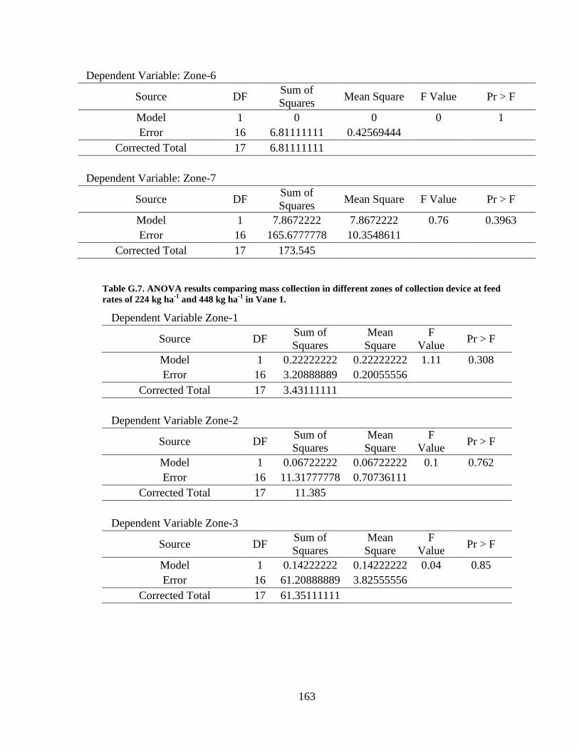
163
Dependent Variable: Zone-6
Source DF Sum of
Squares Mean Square F Value Pr > F
Model 1 0 0 0 1
Error 16 6.81111111 0.42569444
Corrected Total 17 6.81111111
Dependent Variable: Zone-7
Source DF Sum of
Squares Mean Square F Value Pr > F
Model 1 7.8672222 7.8672222 0.76 0.3963
Error 16 165.6777778 10.3548611
Corrected Total 17 173.545
Table G.7. ANOVA results comparing mass collection in different zones of collection device at feed
rates of 224 kg ha-1
and 448 kg ha-1
in Vane 1.
Dependent Variable Zone-1
Source DF Sum of
Squares
Mean
Square
F
Value Pr > F
Model 1 0.22222222 0.22222222 1.11 0.308
Error 16 3.20888889 0.20055556
Corrected Total 17 3.43111111
Dependent Variable Zone-2
Source DF Sum of
Squares
Mean
Square
F
Value Pr > F
Model 1 0.06722222 0.06722222 0.1 0.762
Error 16 11.31777778 0.70736111
Corrected Total 17 11.385
Dependent Variable Zone-3
Source DF Sum of
Squares
Mean
Square
F
Value Pr > F
Model 1 0.14222222 0.14222222 0.04 0.85
Error 16 61.20888889 3.82555556
Corrected Total 17 61.35111111

164
Dependent Variable Zone-4
Source DF Sum of
Squares
Mean
Square
F
Value Pr > F
Model 1 8.26888889 8.26888889 3.17 0.094
Error 16 41.78222222 2.61138889
Corrected Total 17 50.05111111
Dependent Variable Zone-5
Source DF Sum of
Squares
Mean
Square
F
Value Pr > F
Model 1 0.05555556 0.05555556 0.01 0.915
Error 16 75.60444444 4.72527778
Corrected Total 17 75.66
Dependent Variable Zone-6
Source DF Sum of
Squares
Mean
Square
F
Value Pr > F
Model 1 0.045 0.045 0.06 0.817
Error 16 12.98 0.81125
Corrected Total 17 13.025
Dependent Variable Zone-7
Source DF Sum of
Squares
Mean
Square
F
Value Pr > F
Model 1 11.52 11.52 0.26 0.618
Error 16 714.5044444 44.6565278
Corrected Total 17 726.0244444
Table G.8. ANOVA results comparing mass collection in different zones of collection device at three
different spinner disc speeds of 600, 700 and 800 rpm in Vane 1 at feed rate of 224 kg ha-1
.
Dependent Variable Zone-1
Source DF Sum of
Squares
Mean
Square
F
Value Pr > F
Model 2 0.02888889 0.01444444 0.27 0.772
Error 6 0.32 0.05333333
Corrected Total 8 0.34888889

165
Dependent Variable Zone-2
Source DF Sum of
Squares
Mean
Square
F
Value Pr > F
Model 2 3.69555556 1.84777778 10.53 0.011
Error 6 1.05333333 0.17555556
Corrected Total 8 4.74888889
Dependent Variable Zone-3
Source DF Sum of
Squares
Mean
Square
F
Value Pr > F
Model 2 25.62 12.81 12.81 0.007
Error 6 6 1
Corrected Total 8 31.62
Dependent Variable Zone-4
Source DF Sum of
Squares
Mean
Square
F
Value Pr > F
Model 2 11.96222222 5.98111111 26.78 0.001
Error 6 1.34 0.22333333
Corrected Total 8 13.30222222
Dependent Variable Zone-5
Source DF Sum of
Squares
Mean
Square
F
Value Pr > F
Model 2 28.20222222 14.1011111 9.67 0.013
Error 6 8.74666667 1.45777778
Corrected Total 8 36.94888889
Dependent Variable Zone-6
Source DF Sum of
Squares
Mean
Square
F
Value Pr > F
Model 2 7.08666667 3.54333333 77.78 <.0001
Error 6 0.27333333 0.04555556
Corrected Total 8 7.36
Dependent Variable Zone-7
Source DF Sum of
Squares
Mean
Square
F
Value Pr > F
Model 2 319.4022222 159.701111 34.2 5E-04
Error 6 28.02 4.67
Corrected Total 8 347.4222222

166
Table G.9. ANOVA results comparing mass collection in different zones of collection device at three
different spinner disc speeds of 600, 700 and 800 rpm in Vane 1 at feed rate of 448 kg ha-1
.
Dependent Variable Zone-1
Source DF Squares Mean
Square
F
Value Pr > F
Model 2 0.6466667 0.32333333 0.88 0.464
Error 6 2.2133333 0.36888889
Corrected Total 8 2.86
Dependent Variable Zone-2
Source DF Squares Mean
Square
F
Value Pr > F
Model 2 3.1622222 1.58111111 2.78 0.14
Error 6 3.4066667 0.56777778
Corrected Total 8 6.5688889
Dependent Variable Zone-3
Source DF Squares Mean
Square
F
Value Pr > F
Model 2 23.775556 11.8877778 12.27 0.008
Error 6 5.8133333 0.96888889
Corrected Total 8 29.588889
Dependent Variable Zone-4
Source DF Squares Mean
Square
F
Value Pr > F
Model 2 8.4866667 4.24333333 1.27 0.346
Error 6 19.993333 3.33222222
Corrected Total 8 28.48
Dependent Variable Zone-5
Source DF Squares Mean
Square
F
Value Pr > F
Model 2 30.508889 15.2544444 11.23 0.009
Error 6 8.1466667 1.35777778
Corrected Total 8 38.655556
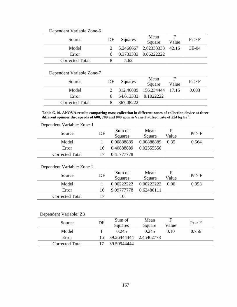
167
Dependent Variable Zone-6
Source DF Squares Mean
Square
F
Value Pr > F
Model 2 5.2466667 2.62333333 42.16 3E-04
Error 6 0.3733333 0.06222222
Corrected Total 8 5.62
Dependent Variable Zone-7
Source DF Squares Mean
Square
F
Value Pr > F
Model 2 312.46889 156.234444 17.16 0.003
Error 6 54.613333 9.1022222
Corrected Total 8 367.08222
Table G.10. ANOVA results comparing mass collection in different zones of collection device at three
different spinner disc speeds of 600, 700 and 800 rpm in Vane 2 at feed rate of 224 kg ha-1
.
Dependent Variable: Zone-1
Source DF Sum of
Squares
Mean
Square
F
Value Pr > F
Model 1 0.00888889 0.00888889 0.35 0.564
Error 16 0.40888889 0.02555556
Corrected Total 17 0.41777778
Dependent Variable: Zone-2
Source DF Sum of
Squares
Mean
Square
F
Value Pr > F
Model 1 0.00222222 0.00222222 0.00 0.953
Error 16 9.99777778 0.62486111
Corrected Total 17 10
Dependent Variable: Z3
Source DF Sum of
Squares
Mean
Square
F
Value Pr > F
Model 1 0.245 0.245 0.10 0.756
Error 16 39.26444444 2.45402778
Corrected Total 17 39.50944444

168
Dependent Variable: Zone-4
Source DF Sum of
Squares
Mean
Square
F
Value Pr > F
Model 1 3.7355556 3.7355556 0.58 0.456
Error 16 102.1822222 6.3863889
Corrected Total 17 105.9177778
Dependent Variable: Zone-5
Source DF Sum of
Squares
Mean
Square
F
Value Pr > F
Model 1 0.20055556 0.20055556 0.09 0.774
Error 16 37.66888889 2.35430556
Corrected Total 17 37.86944444
Dependent Variable: Zone-6
Source DF Sum of
Squares
Mean
Square
F
Value Pr > F
Model 1 0 0.00000000 0.00 1
Error 16 6.81111111 0.42569444
Corrected Total 17 6.81111111
Dependent Variable: Zone-7
Source DF Sum of
Squares
Mean
Square
F
Value Pr > F
Model 1 7.8672222 7.8672222 0.76 0.396
Error 16 165.6777778 10.3548611
Corrected Total 17 173.545
Table G.11. ANOVA results comparing mass collection in different zones of collection device at three
different spinner disc speeds of 600, 700 and 800 rpm in Vane 2 at feed rate of 448 kg ha-1
.
Dependent Variable Zone-1
Source DF Sum of
Squares Mean Square
F
Value Pr > F
Model 2 0.04222222 0.02111111 2.71 0.1447
Error 6 0.04666667 0.00777778
Corrected Total 8 0.08888889

169
Dependent Variable Zone-2
Source DF Sum of
Squares Mean Square
F
Value Pr > F
Model 2 1.62888889 0.81444444 3.15 0.1163
Error 6 1.55333333 0.25888889
Corrected Total 8 3.18222222
Dependent Variable Zone-3
Source DF Sum of
Squares Mean Square
F
Value Pr > F
Model 2 15.61555556 7.80777778 5.43 0.0451
Error 6 8.63333333 1.43888889
Corrected Total 8 24.24888889
Dependent Variable Zone-4
Source DF Sum of
Squares Mean Square
F
Value Pr > F
Model 2 30.86222222 15.43111111 2.19 0.1935
Error 6 42.34 7.05666667
Corrected Total 8 73.20222222
Dependent Variable Zone-5
Source DF Sum of
Squares Mean Square
F
Value Pr > F
Model 2 10.40666667 5.20333333 3.56 0.0957
Error 6 8.77333333 1.46222222
Corrected Total 8 19.18
Dependent Variable Zone-6
Source DF Sum of
Squares Mean Square
F
Value Pr > F
Model 2 1.82888889 0.91444444 5.34 0.0465
Error 6 1.02666667 0.17111111
Corrected Total 8 2.85555556
Dependent Variable Zone-7
Source DF Sum of
Squares Mean Square
F
Value Pr > F
Model 2 16.89555556 8.44777778 0.72 0.5246
Error 6 70.41333333 11.73555556
Corrected Total 8 87.30888889

170
Table G.12. ANOVA results comparing mass collection in different zones of collection device at feed
rates of 224 kg ha-1
and 448 kg ha-1
in Vane 3.
Dependent Variable Zone-1
Source DF Sum of
Squares
Mean
Square
F
Value Pr > F
Model 1 0 0.00000000 0.00 1
Error 16 0.47111111 0.02944444
Corrected Total 17 0.47111111
Dependent Variable Zone-2
Source DF Sum of
Squares
Mean
Square
F
Value Pr > F
Model 1 0.68055556 0.68055556 0.74 0.403
Error 16 14.75555556 0.92222222
Corrected Total 17 15.43611111
Dependent Variable Zone-3
Source DF Sum of
Squares
Mean
Square
F
Value Pr > F
Model 1 0.1605556 0.1605556 0.02 0.882
Error 16 112.4955556 7.0309722
Corrected Total 17 112.6561111

171
Dependent Variable Zone-4
Source DF Sum of
Squares
Mean
Square
F
Value Pr > F
Model 1 0.03555556 0.03555556 0.02 0.895
Error 16 31.74222222 1.98388889
Corrected Total 17 31.77777778
Dependent Variable Zone-5
Source DF Sum of
Squares
Mean
Square
F
Value Pr > F
Model 1 2 2.00000000 0.25 0.621
Error 16 126.0311111 7.8769444
Corrected Total 17 128.0311111
Dependent Variable Zone-6
Source DF Sum of
Squares
Mean
Square
F
Value Pr > F
Model 1 0.09388889 0.09388889 0.11 0.741
Error 16 13.28888889 0.83055556
Corrected Total 17 13.38277778
Dependent Variable Zone-7
Source DF Sum of
Squares
Mean
Square
F
Value Pr > F
Model 1 0.2222222 0.2222222 0.01 0.941
Error 16 636.9577778 39.8098611
Corrected Total 17 637.18
Table G.13. ANOVA results comparing mass collection in different zones of collection device at three
different spinner disc speeds of 600, 700 and 800 rpm in Vane 3 at feed rate of 224 kg ha-1
.
Dependent Variable Zone-1
Source DF Sum of
Squares
Mean
Square
F
Value Pr > F
Model 2 0.16222222 0.08111111 2.28 0.183
Error 6 0.21333333 0.03555556
Corrected Total 8 0.37555556
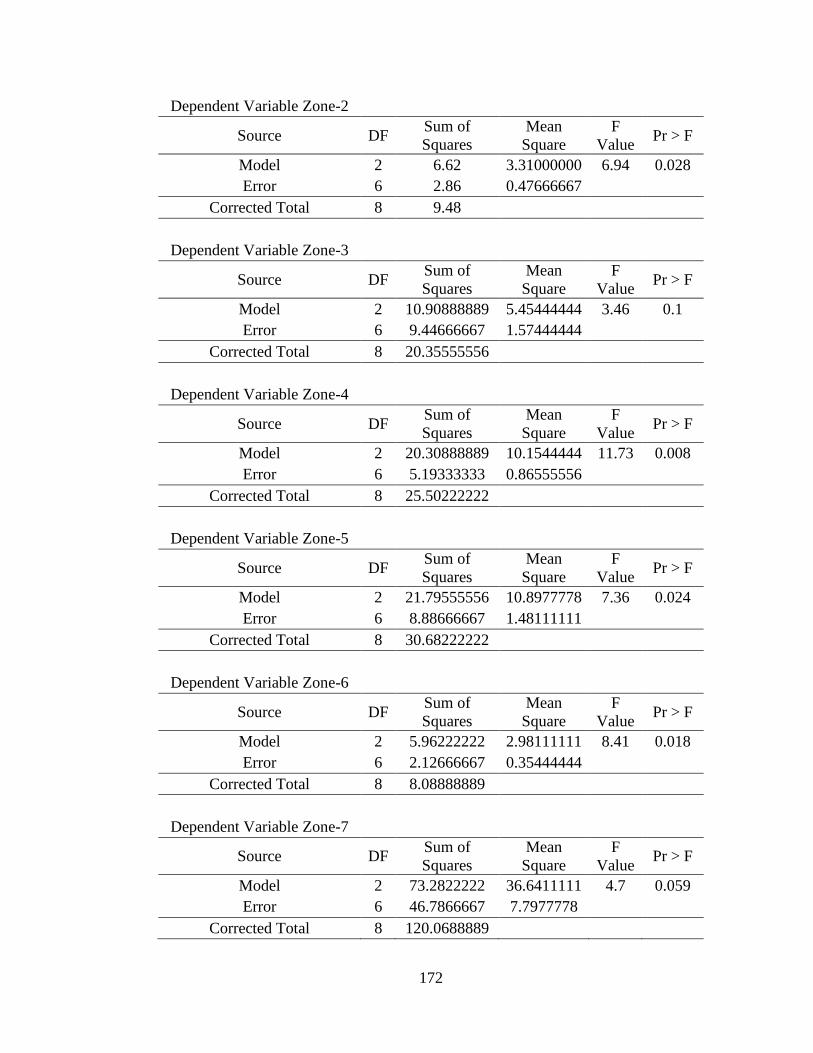
172
Dependent Variable Zone-2
Source DF Sum of
Squares
Mean
Square
F
Value Pr > F
Model 2 6.62 3.31000000 6.94 0.028
Error 6 2.86 0.47666667
Corrected Total 8 9.48
Dependent Variable Zone-3
Source DF Sum of
Squares
Mean
Square
F
Value Pr > F
Model 2 10.90888889 5.45444444 3.46 0.1
Error 6 9.44666667 1.57444444
Corrected Total 8 20.35555556
Dependent Variable Zone-4
Source DF Sum of
Squares
Mean
Square
F
Value Pr > F
Model 2 20.30888889 10.1544444 11.73 0.008
Error 6 5.19333333 0.86555556
Corrected Total 8 25.50222222
Dependent Variable Zone-5
Source DF Sum of
Squares
Mean
Square
F
Value Pr > F
Model 2 21.79555556 10.8977778 7.36 0.024
Error 6 8.88666667 1.48111111
Corrected Total 8 30.68222222
Dependent Variable Zone-6
Source DF Sum of
Squares
Mean
Square
F
Value Pr > F
Model 2 5.96222222 2.98111111 8.41 0.018
Error 6 2.12666667 0.35444444
Corrected Total 8 8.08888889
Dependent Variable Zone-7
Source DF Sum of
Squares
Mean
Square
F
Value Pr > F
Model 2 73.2822222 36.6411111 4.7 0.059
Error 6 46.7866667 7.7977778
Corrected Total 8 120.0688889

173
Table G.14. ANOVA results comparing mass collection in different zones of collection device at three
different spinner disc speeds of 600, 700 and 800 rpm in Vane 3 at feed rate of 448 kg ha-1
.
Dependent Variable Zone-1
Source DF Sum of
Squares
Mean
Square
F
Value Pr > F
Model 2 0.02888889 0.01444444 1.3 0.34
Error 6 0.06666667 0.01111111
Corrected Total 8 0.09555556
Dependent Variable Zone-2
Source DF Sum of
Squares
Mean
Square
F
Value Pr > F
Model 2 4.49555556 2.24777778 17.29 0.003
Error 6 0.78 0.13000000
Corrected Total 8 5.27555556
Dependent Variable Zone-3
Source DF Sum of
Squares
Mean
Square
F
Value Pr > F
Model 2 88.66666667 44.3333333 76.58 <.0001
Error 6 3.47333333 0.57888889
Corrected Total 8 92.14
Dependent Variable Zone-4
Source DF Sum of
Squares
Mean
Square
F
Value Pr > F
Model 2 0.26 0.13000000 0.13 0.88
Error 6 5.98 0.99666667
Corrected Total 8 6.24
Dependent Variable Zone-5
Source DF Sum of
Squares
Mean
Square
F
Value Pr > F
Model 2 88.73555556 44.3677778 40.25 3E-04
Error 6 6.61333333 1.10222222
Corrected Total 8 95.34888889

174
Dependent Variable Zone-6
Source DF Sum of
Squares
Mean
Square
F
Value Pr > F
Model 2 3.54666667 1.77333333 6.44 0.032
Error 6 1.65333333 0.27555556
Corrected Total 8 5.2
Dependent Variable Zone-7
Source DF Sum of
Squares
Mean
Square
F
Value Pr > F
Model 2 508.2422222 254.121111 176.34 <.0001
Error 6 8.6466667 1.4411111
Corrected Total 8 516.8888889
Table G.15. ANOVA results comparing mass collection in different zones of collection device at feed
rates of 224 kg ha-1
and 448 kg ha-1
in Vane 4.
Dependent Variable Zone-1
Source DF Sum of
Squares
Mean
Square
F
Value Pr > F
Model 1 0.01388889 0.01388889 0.22 0.643
Error 16 0.99555556 0.06222222
Corrected Total 17 1.00944444
Dependent Variable Zone-2
Source DF Sum of
Squares
Mean
Square
F
Value Pr > F
Model 1 0.03555556 0.03555556 0.07 0.797
Error 16 8.32444444 0.52027778
Corrected Total 17 8.36
Dependent Variable Zone-3
Source DF Sum of
Squares
Mean
Square
F
Value Pr > F
Model 1 0.125 0.1250000 0.05 0.83
Error 16 41.79777778 2.61236111
Corrected Total 17 41.92277778

175
Dependent Variable Zone-4
Source DF Sum of
Squares
Mean
Square
F
Value Pr > F
Model 1 1.50222222 1.50222222 0.47 0.504
Error 16 51.48222222 3.21763889
Corrected Total 17 52.98444444
Dependent Variable Zone-5
Source DF Sum of
Squares
Mean
Square
F
Value Pr > F
Model 1 0.00055556 0.00055556 0 0.991
Error 16 62.21555556 3.88847222
Corrected Total 17 62.21611111
Dependent Variable Zone-6
Source DF Sum of
Squares
Mean
Square
F
Value Pr > F
Model 1 0.00888889 0.00888889 0.02 0.896
Error 16 8.07555556 0.50472222
Corrected Total 17 8.08444444
Dependent Variable Zone-7
Source DF Sum of
Squares
Mean
Square
F
Value Pr > F
Model 1 0.98 0.98 0.08 0.785
Error 16 204.46 12.77875
Corrected Total 17 205.44
Table G.16. ANOVA results comparing mass collection in different zones of collection device at three
different spinner disc speeds of 600, 700 and 800 rpm in Vane 4 at feed rate of 224 kg ha-1
.
Dependent Variable Zone-1
Source DF Sum of
Squares
Mean
Square
F
Value Pr > F
Model 2 0.02 0.01000000 1.5 0.296
Error 6 0.04 0.00666667
Corrected Total 8 0.06

176
Dependent Variable Zone-2
Source DF Sum of
Squares
Mean
Square
F
Value Pr > F
Model 2 0.06222222 0.03111111 0.06 0.945
Error 6 3.28666667 0.54777778
Corrected Total 8 3.34888889
Dependent Variable Zone-3
Source DF Sum of
Squares
Mean
Square
F
Value Pr > F
Model 2 12.76222222 6.38111111 11.33 0.009
Error 6 3.38 0.56333333
Corrected Total 8 16.14222222
Dependent Variable Zone-4
Source DF Sum of
Squares
Mean
Square
F
Value Pr > F
Model 2 3.38 1.69000000 0.88 0.463
Error 6 11.56 1.92666667
Corrected Total 8 14.94
Dependent Variable Zone-5
Source DF Sum of
Squares
Mean
Square
F
Value Pr > F
Model 2 19.62 9.81 15.82 0.004
Error 6 3.72 0.62
Corrected Total 8 23.34
Dependent Variable Zone-6
Source DF Sum of
Squares
Mean
Square
F
Value Pr > F
Model 2 0.38888889 0.19444444 0.36 0.711
Error 6 3.22666667 0.53777778
Corrected Total 8 3.61555556
Dependent Variable Zone-7
Source DF Sum of
Squares
Mean
Square
F
Value Pr > F
Model 2 100.4466667 50.2233333 12.47 0.007
Error 6 24.1733333 4.0288889
Corrected Total 8 124.62

177
Table G.17. ANOVA results comparing mass collection in different zones of collection device at three
different spinner disc speeds of 600, 700 and 800 rpm in Vane 4 at feed rate of 448 kg ha-1
.
Dependent Variable Zone-1
Source DF Sum of
Squares
Mean
Square
F
Value Pr > F
Model 2 0.27555556 0.13777778 1.25 0.351
Error 6 0.66 0.11000000
Corrected Total 8 0.93555556
Dependent Variable Zone-2
Source DF Sum of
Squares
Mean
Square
F
Value Pr > F
Model 2 1.62888889 0.81444444 1.46 0.304
Error 6 3.34666667 0.55777778
Corrected Total 8 4.97555556
Dependent Variable Zone-3
Source DF Sum of
Squares
Mean
Square
F
Value Pr > F
Model 2 4.00222222 2.00111111 0.55 0.601
Error 6 21.65333333 3.60888889
Corrected Total 8 25.65555556
Dependent Variable Zone-4
Source DF Sum of
Squares
Mean
Square
F
Value Pr > F
Model 2 16.64888889 8.32444444 2.51 0.161
Error 6 19.89333333 3.31555556
Corrected Total 8 36.54222222
Dependent Variable Zone-5
Source DF Sum of
Squares
Mean
Square
F
Value Pr > F
Model 2 5.70888889 2.85444444 0.52 0.621
Error 6 33.16666667 5.52777778
Corrected Total 8 38.87555556

178
Dependent Variable Zone-6
Source DF Sum of
Squares
Mean
Square
F
Value Pr > F
Model 2 1.26 0.63000000 1.18 0.369
Error 6 3.2 0.53333333
Corrected Total 8 4.46
Dependent Variable Zone-7
Source DF Sum of
Squares
Mean
Square
F
Value Pr > F
Model 2 5.40666667 2.70333333 0.22 0.81
Error 6 74.43333333 12.4055556
Corrected Total 8 79.84