1

Effect of initial condition on subsonic jet noise from two

rectangular nozzles

K.B.M.Q. Zaman1

NASA Glenn Research Center

Cleveland, OH 44135

Abstract

Differences in jet noise data from two small 8:1 aspect ratio nozzles are investigated experimentally. The

interiors of the two nozzles are identical but one has a thin-lip at the exit while the has a perpendicular

face at the exit (thick-lip). It is found that the thin-lip nozzle is substantially noisier throughout the

subsonic Mach number range. As much as 5dB difference in OASPL is noticed around Mj =0.96. Hot-

wire measurements are carried out for the characteristics of the exit boundary layer and, overall, the noise

difference can be ascribed to differences in the boundary layer state. The boundary layer of the quieter

(thick-lip) nozzle goes through transition around Mj =0.25 and at higher Mj it remains „nominally

turbulent‟. In comparison, the boundary layer of the thin-lip nozzle is found to remain „nominally

laminar‟ at high subsonic conditions. The nominally laminar state involves significantly larger turbulence

intensities commensurate with the higher radiated noise.

1. Introduction

Substantial differences in subsonic jet noise databases have been reported in [1, 2]. It was noted that data

taken in cleaner „University-type‟ facilities [3-6] were actually noisier relative to data taken in „Industrial-

type‟ facilities [1, 7, 8]. In [9] another pertinent observation was made; two round nozzles of same exit

diameter but different internal geometry („ASME‟ versus „Conic‟), tested in the same facility, displayed a

significant difference in the noise spectra. These anomalies were addressed recently in an experimental

study at NASA Glenn Research Center (GRC). With two nozzles of the same internal geometries as in

[9] the difference in the noise spectra could be reproduced and a possible reason for the difference could

be traced to the initial boundary layer state. The noisier ASME nozzle involved a „nominally laminar‟

efflux boundary layer whereas the quieter Conic nozzle was characterized by a „nominally turbulent‟

boundary layer. The former boundary layer state actually involved significantly larger turbulence

intensities reconciling with the higher radiated noise. These results were presented at the last AIAA

Aeroacoustics meeting [10]. In view of the importance of the subject the study was continued and further

data were obtained with the same two round nozzles beyond those covered in [10] (a revised version of

the paper with additional results is to appear in the AIAA Journal). The key results for this pair of round

nozzles are first reviewed in the following in order to orient the reader with the problem at hand.

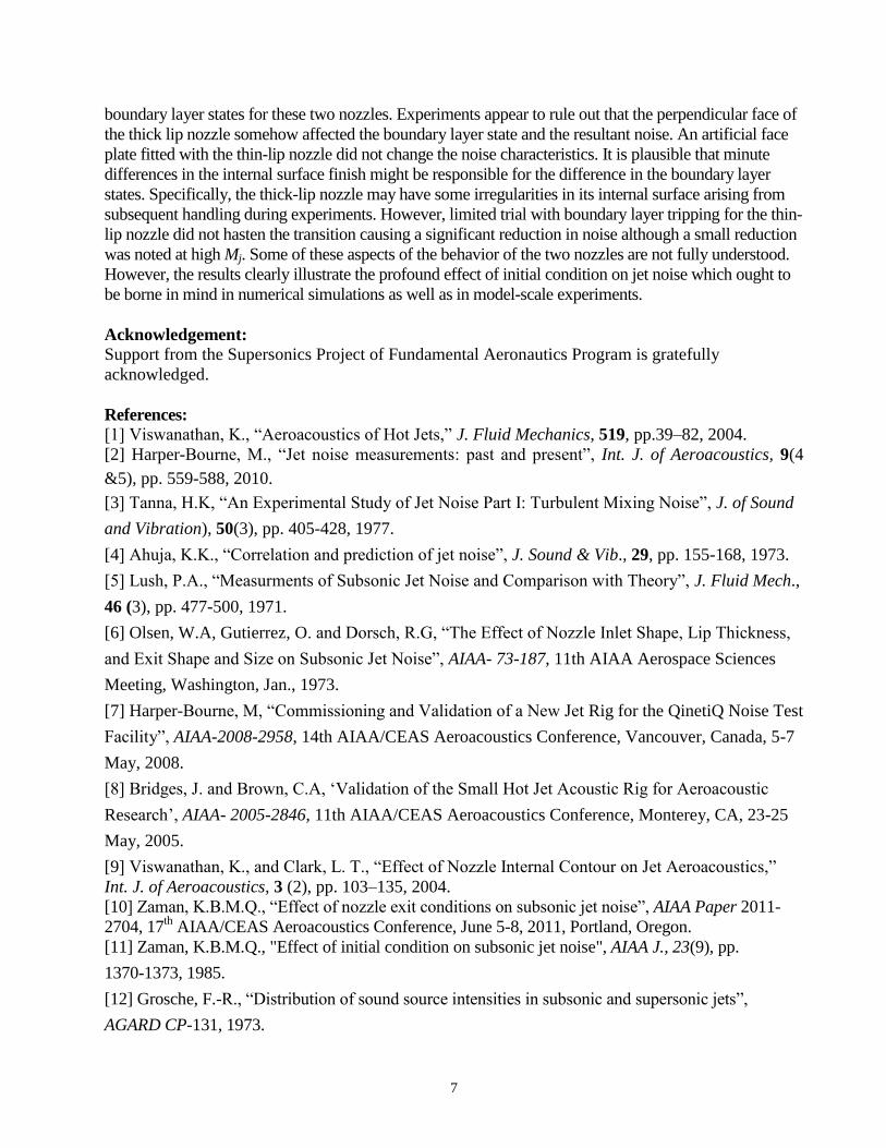
The contours of the ASME and Conic nozzles are shown in Fig. 1. Sound pressure level (SPL) spectra

showing the amplitude difference between the two nozzles, first reported in [9], is shown in Fig. 2(a).

The current data, as reported in [10], are shown in Fig. 2(b). It can be seen that in either study the ASME

nozzle had significantly larger amplitudes on the high frequency end of the spectra. It was then

demonstrated that the noisier (ASME) nozzle involved a highly disturbed laminar, or „nominally

laminar‟, boundary layer state as opposed to a turbulent state with the other (Conic) nozzle. Exit

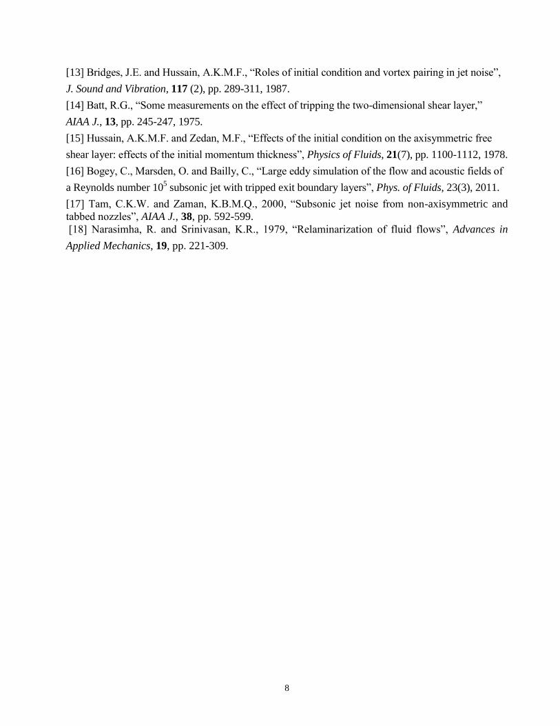
boundary layer momentum thickness variation with jet Mach number (and Reynolds number based on

1 Inlet & Nozzle Branch, Aeropropulsion Division, AIAA Associate Fellow.

https://ntrs.nasa.gov/search.jsp?R=20120014298 2020-05-26T09:28:46+00:00Z

2

nozzle diameter) for the two nozzles are compared in Fig. 3. It can be seen that the Conic nozzle goes

through a transition around Mj = 0.3, as marked by a sudden jump in the thickness. In comparison the

boundary layer for the ASME nozzle approximately follows laminar prediction throughout the entire

subsonic range. Furthermore, the nominally laminar boundary layer (ASME) is actually marked by larger

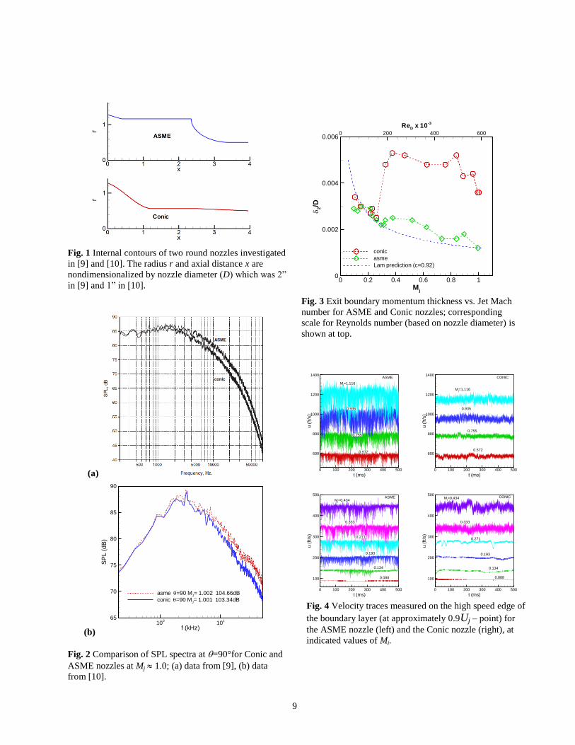
turbulence intensities consistent with the higher radiated noise. The difference is vividly illustrated in Fig.

4 by velocity traces obtained at the high-speed edge of the boundary layer. The ASME and the Conic

nozzle data are shown on the left and right columns, respectively (for clarity the data are split in two sets

in each column). The traces are shown side-by-side for comparable jet Mach numbers (Mj). After

„transition‟ at Mj 0.134 the intensities for the ASME case are found to be larger, relative to the Conic

case, all the way up to the highest Mj covered in the experiment (the issue of „transition‟ is discussed

later). The characteristics of the velocity signals are also different. The nominally laminar (ASME) case

exhibits large amplitude negative spikes as opposed to the smaller amplitude random fluctuations with

the turbulent (Conic) case. These results illustrate the difference in the boundary layer states and its

correspondence to the difference in radiated noise for the pair of nozzles considered.

The characteristics of various boundary layer states were discussed in earlier publications [10, 11] and

these are not repeated here. An interested reader may also look up the following citations. The effect of

boundary layer state on jet noise and its flow fields has been studied experimentally, e.g., in [11-15] and

more recently by numerical simulations, e.g., in [16]. While boundary layer states were not measured

together with the jet noise databases, as discussed at the beginning of this introduction section, it is

possible that differences therein might explain the noted anomaly in noise. Specifically, the „University

type facilities‟ might have had nominally laminar boundary layers consistent with the higher radiated

noise observed with them.

In the present paper we turn our attention to a pair of small rectangular nozzles. The objective is to

explore the differences in the noise radiation noted in connection with a past work [17]. The anomaly

could not be explained at that time and had remained a mystery. The noise radiation from the two 8:1

aspect ratio nozzles was re-examined and the difference was confirmed. As to be shown in the following,

a similar difference in the initial boundary layer state (as with the ASME and Conic cases) is found to

exist between these two nozzles. However, while the ASME and the Conic nozzles had difference in

internal contours that qualitatively explained the difference in their boundary layer states (discussed

further in the following), the internal contours of the two rectangular nozzles were identical. The

difference in the boundary layer state could not be satisfactorily explained even though various

possibilities were explored. In any case, the results for these two nozzles, once again, provide evidence

that initial boundary layer state can make a profound impact on jet noise. These results are summarized in

the following.

2. Experimental Facility and Procedure

All data were taken in an open jet facility at GRC. Compressed air passed through a 30 inch

diameter plenum chamber and exhausted through the nozzle into the ambient of the test chamber.

With the large contraction ratio and flow conditioning units within the plenum, this facility falls into

the category of „University type‟ in the terminology of [2]. (However, the facility type is immaterial

since the noise and flow differences are studied in the same facility and are obviously tied to

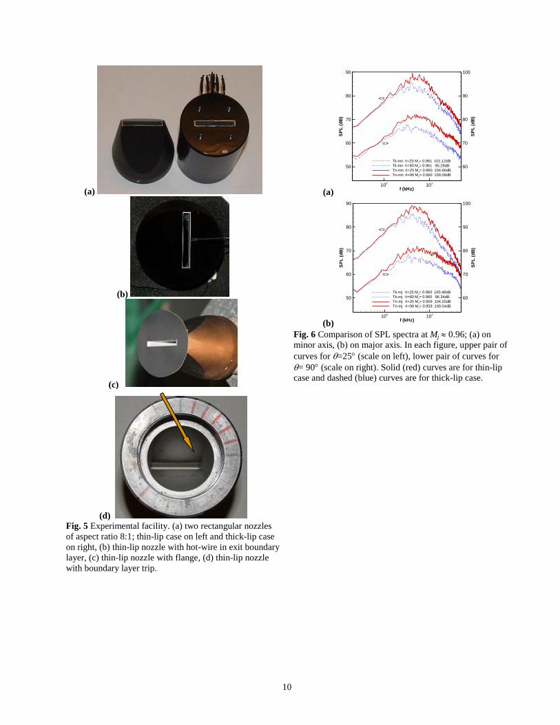
differences in the nozzles themselves). The two rectangular nozzles are shown in Fig. 5(a). They

could be attached to the plenum chamber via a fixed receptacle. The two nozzles were fabricated by

electrical discharge machining (EDM) using the same plunger and thus have identical internal

3

contours. The aspect ratio at the exit is 8:1 and the equivalent diameter based on exit area is 0.58

inch. Each has a 0.6 inch long section at the end with constant cross-sectional shape in order to

provide parallel flow-lines at the exit. The difference is in the external geometry. The nozzle on the

left has thin lip all around (approximately 0.025 inch thick). The one on the right has „thick‟ lip, i.e.,

it discharges through a perpendicular face. (For the latter nozzle, the four screw holes on the face, used

simply to attach a plate to hold tabs [17], were filled for this experiment and may be ignored. There are

nine 0.010 inch diameter static pressure taps on one side – five placed laterally 0.2 inch upstream of the

exit and the other four placed axially along the center extending into the contracting section. These were

blocked from outside and also thought to be inconsequential for this investigation.)

The boundary layer measurements were done with a single hot-wire (TSI 1260-A10) at approximately

0.03 inch downstream from the nozzle lip. The probe was mounted on an automated computer-controlled

traversing mechanism and was inserted in the flow at an angle. Only the tip of the probe entered the flow.

Figure 5(b) shows the thin-lip nozzle with the probe placed at about 90% velocity point in the boundary

layer; this picture was taken during an investigation of the effect of the probe itself on the noise field.

Figure 5(c) shows a picture of the thin-lip nozzle fitted with a flange at the end in an effort to mimick the

exit face of the thick-lip nozzle. The flange was flush with the lip and epoxied from the back and the

purpose was to explore if simply the presence of the perpendicular face would explain the difference in

the noise. Figure 5(d) shows a rear view of the thin-lip nozzle with internal boundary layer trips. The

tripping was explored, again, in an effort to understand the source of the noise difference. The trip

consisted of four hemispherical epoxy beads placed on each long side, towards the end of the contracting

section and just prior to the parallel section. The beads were approximately 0.08 inch in diameter and

0.03 inch high, making sure that they were far enough downstream yet not too close to the parallel

section to alter the exit area. The beads are barely visible in the picture, the yellow arrow points to the

location of one.

Sound pressure level spectra were measured with ¼-inch (B&K) microphones placed at polar

locations ( = ) 25° and 90° relative to the jet‟s (downstream) axis. All experiments involved „cold‟

flows, i.e., unheated flows with total temperature the same throughout and equal to that in the

ambient. The „fully expanded jet Mach number‟, 2/1/)1(

0 )1

2)1)/(((

aj ppM , is used as the

independent variable; p0 and pa are plenum pressure and ambient pressure, respectively.

3. Results:

The thin-lip nozzle exhibited higher noise and this is shown in Fig. 6 with sound pressure level spectra

measured at Mj =0.96. The microphone is located on the minor axis for the data in (a) and on the major

axis for the data in (b). In each figure, data for = 25° and 90° are compared for the two nozzles and the

graphs are explained in the figure caption. It can be seen that at =90°, the spectral levels for the thin-lip

nozzle are larger by over 6 dB on the high frequency end. The levels for this nozzle are also higher at 25°

practically over the entire frequency range. Essentially the same difference is seen in both Figs. 6(a) and

(b). Thus, the thin-lip nozzle is louder in both major and minor axis planes, at both angular locations as

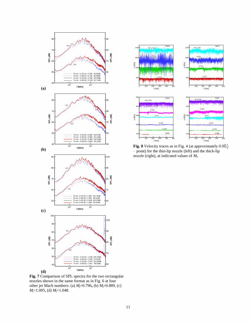
well as practically over the entire frequency range. Further noise spectral data are shown in Figs. 7(a)-(d)

for additional Mj values of 0.796, 0.889, 1.005 and 1.048. It can be seen that the noise difference persists

throughout the high subsonic regime. The difference has become less at Mj =1.048 when a screech tone

has appeared at about 42 kHz for the thick-lip nozzle (blue dotted curves).

4

Boundary layer measurements were done for the two nozzles at the middle of the long edge. Let us begin

with comparison of velocity traces similar to those shown in Fig. 4. The (noisier) thin-lip nozzle data are

shown on the left column while those for the thick-lip nozzle are shown on the right column. For the

thick-lip case boundary layer transition can be noted at about Mj = 0.271, above which the velocity

fluctuations appear random as seen with the Conic nozzle in Fig. 4. In comparison, „transition‟ has taken

place at a somewhat higher Mj for the thin-lip nozzle; (the word transition is put under quotes since it did

not result in a thickening of the boundary layer typical of turbulent state as with the other nozzle, to be

discussed further shortly). At even higher Mj, the velocity fluctuation amplitudes are larger for the thin-lip

case and also marked by the negative spikes, similar to that seen with the ASME nozzle in Fig. 4. Note

that at the highest Mj (=1.116) the amplitudes have become comparable for the two nozzles. Details of

these trends become clearer with further boundary layer data shown in the following.

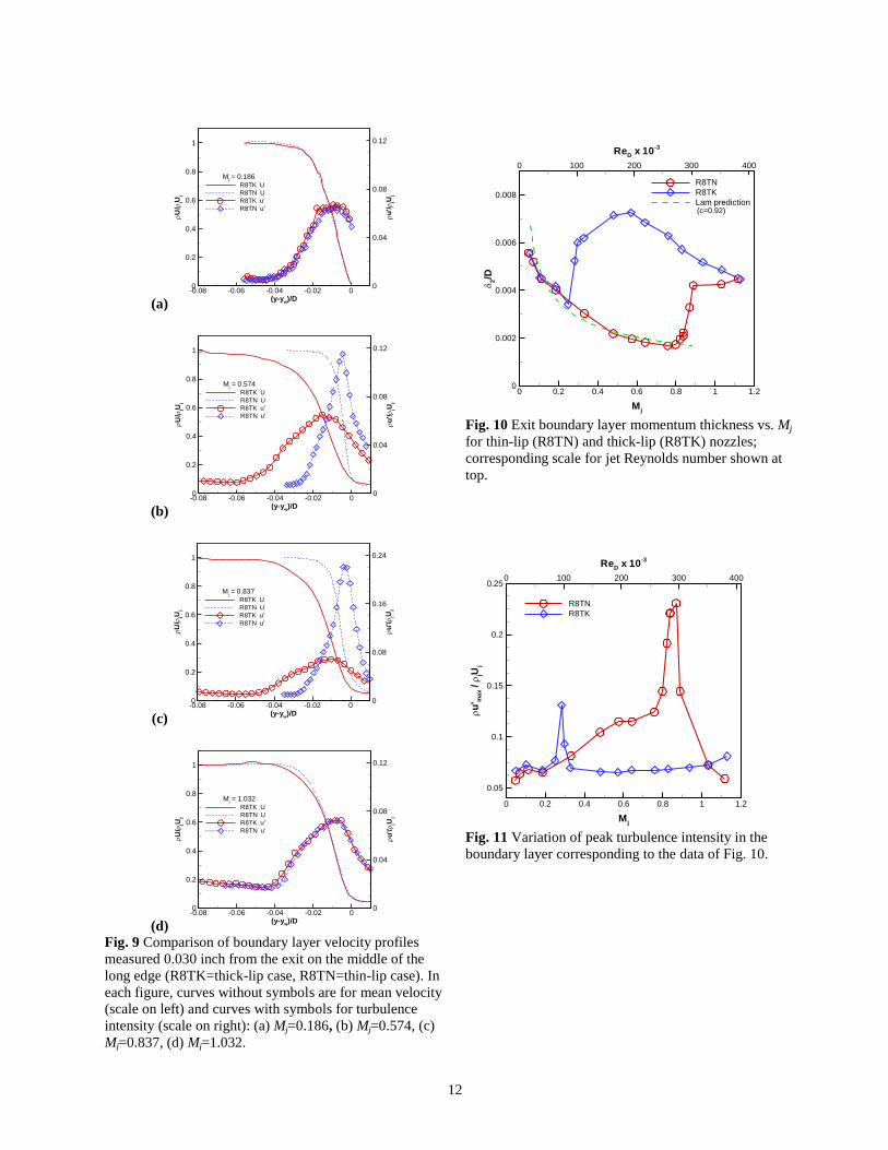
Examples of velocity profiles at four values of Mj are shown in Fig. 9. Here, U and u’ are axial mean

velocity and turbulence intensity and is density with subscript „j‟ denoting conditions at the nozzle exit

center; y is the radial coordinate and yw is the nozzle wall location estimated from extrapolation of the

measured U - profile. In each figure, the curves without data points are U - profiles (with scale on left)

while the curves with data points represent u’- profiles (with scale on right). (Note that at higher Mach

numbers for compressible flow the hot-wire responds to a combination of velocity and density; with

constant temperature operation of the anemometer the response is less sensitive to temperature [10]. At

low Mj the profiles represent U/Uj and u’/Uj but at higher Mj the profiles qualitatively represent the

product of density and velocity.) At Mj =0.186, the boundary layer for either nozzle is nominally laminar

and the U- as well as u’-profiles are practically identical. At Mj =0.574, the boundary layer for the thin-lip

case has remained thin while for the thick-lip case transition has taken place as indicated by a much

thicker boundary layer. The turbulence intensity for the former case, however, has become larger. At Mj

=0.837, the difference in the mean velocity profiles persists, however, the turbulence intensity has

become enormous (note the doubling of the scale on the right). At the highest Mj of 1.032, apparently the

boundary layer for the thin-lip case has also gone through full transition and the mean velocity profiles

for the two nozzles have become similar. The turbulence intensity for the thin-lip case has dropped and

become almost identical to that of the other nozzle. These trends are further illustrated via integral

properties based on profiles measured at many more values of Mj.

Comparison of boundary layer momentum thickness variation is shown in Fig. 10 in the same format as

in Fig. 3. Clearly, the thick-lip nozzle went through boundary layer transition around Mj =0.25, (similar to

the Conic case in Fig. 3). On the other hand, the thin-lip nozzle continued to have nominally laminar

boundary layer up to about Mj =0.85. At higher Mj, the rapid rise in the boundary layer thickness for the

latter nozzle suggests „transition‟ to turbulent state; recall from Fig. 8 an earlier „transition‟ took place for

this nozzle at about Mj =0.3. Recall also that the noise discrepancy persisted at Mj higher than 0.85 (Figs.

6 and 7), an issue discussed further shortly. Peak turbulence intensity, corresponding to the data of Fig.

10, is compared in Fig. 11. For either nozzle, the turbulence becomes high shortly before transition to full

turbulence – resulting in the peaks at Mj 0.3 and 0.85 for the thick- and thin-lip cases, respectively. Over

the Mj -range of approximately 0.3-1.0, turbulence is larger for the thin-lip case. This is approximately the

range where noise is also higher for this nozzle.

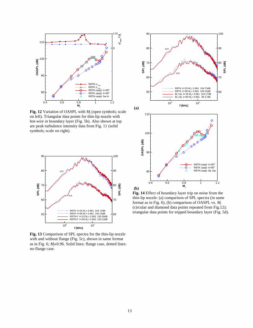
The overall sound pressure levels (OASPL) obtained by integration of the SPL spectra are compared for

the two nozzles in Fig. 12 (open symbols). These data are for a polar location of =90; (a similar trend is

also seen at =25). Also shown on the top of Fig. 12 is the comparison of the peak turbulence intensity

curves copied from Fig. 11 (solid symbols, with scale on right). The OASPL data show that the thin-lip

5

nozzle is clearly noisier over the Mj-range of about 0.6 -1.0. The maximum difference is noted around Mj

0.95. On the other hand, the maximum difference in the peak turbulence intensity occurs at Mj 0.85!

So far the results from both the round nozzle pair and the rectangular nozzle pair were consistent – higher

noise was associated with higher turbulence in the boundary layer. The mismatch of jet Mach number for

the occurrence of maximum difference in turbulence and in noise has deviated from that simple trend.

The thought occurred that, perhaps, the intrusion of the hot-wire in the thin-lip nozzle case tripped its

boundary layer at about Mj=0.85. All noise data shown so far were taken with the hot-wire out of the

flow. In order to test this possibility, noise data were retaken for the thin-lip nozzle with the hot-wire

placed in the boundary layer (Fig. 5b). Corresponding OASPL data are shown by the triangular (cyan)

symbols in Fig. 12. These data fall on the top of the earlier data. This rules out the possibility of hot-wire

itself acting as a trip for Mj >0.85.

Recall that the difference between the ASME and Conic nozzles was in the internal contours (Fig. 1). The

rapid contraction in the elliptical section of the ASME nozzle created a thin laminar boundary layer that

did not get a chance to grow enough to allow transition within the subsequent cylindrical section. In fact,

calculation of an acceleration parameter62 10/ U

dx

dUK , following [18], yielded values over 600

near the entrance of the elliptical section, dropping below 2 past 0.91D upstream from the nozzle exit.

A value of K=2 was noted in the cited reference to be the threshold below which a turbulent state

would be sustained and above which relaminarization would occur. Comparatively, the value of K was

only about 0.35 throughout the conical section of the Conic nozzle. While far from a complete

explanation, this qualitatively reconciled the nominally laminar state with the ASME nozzle and a

turbulent state with the Conic nozzle.

The dilemma with the two rectangular nozzles is that the internal contours are identical. Thus, flow

acceleration does not explain the difference in the boundary layer states. An obvious geometrical

difference between the two is the perpendicular face with the thick-lip case. It was thought that perhaps

the entrainment pattern for this case created a low pressure at the exit thus subjecting the boundary layer

near the exit to a favorable pressure gradient. Note that the slight taper with the Conic nozzle, the one

exhibiting similar boundary layer state as the thick-lip nozzle, also created a favorable pressure gradient

near the exit. In order to test if the perpendicular face was somehow responsible for the observed

difference, a flange was fabricated to fit over the thin-lip nozzle (Fig. 5c). Noise data were acquired with

this configuration for several Mj. An example is shown in Fig. 13 comparing with earlier (no flange) data.

No significant change in the spectra could be discerned. Thus, the perpendicular face affecting the exit

boundary layer (and in turn the noise) does not seem to be the source for the observed differences.

The rectangular nozzles were fabricated many years ago. Even though the interiors looked similar upon

visual inspection it is possible some changes occurred within the internal surfaces due to handling during

the experiments. The pressure taps with the thick-lip nozzle (§2) also constituted a difference between the

two (the thin-lip nozzle did not have such taps). Boundary layer tripping was not tried so far in order to

preserve the interiors so that the results could be repeated during the investigation. It appears that with

appropriate tripping one should be able to change the nominally laminar state with the thin-lip case to a

turbulent state. This was tried at the end of all experiments. The method of tripping was described earlier

6

with the help of Fig. 5(d). Noise measurements were repeated with the tripped nozzle and an example of

SPL spectra is shown in Fig. 14(a), comparing with data taken earlier without tripping. On a first look,

there does not seem to be much difference. Upon a scrutiny, some reduction in the amplitudes can be

noticed for the tripped case. For example, the OASPL (noted in the last column of the legend) at 90˚ has

dropped by almost 1 dB. The variation of OASPL as a function of Mj is compared in Fig. 14(b). The

circular and diamond symbols are repeats from Fig. 12 for the thin- and thick-lip cases, respectively. The

triangular symbols represent data taken with the tripped thin-lip nozzle. A small but consistent reduction

in OASPL can be noticed around Mj.0.95. However, the tripping obviously has failed to bring the levels

far enough down to match the data for the thick-lip case. This indicates that the tripping affected the

boundary layer only slightly at the high end of the Mj range and failed to trigger full transition. It

underscores the difficulties in boundary layer tripping which often takes trial and error. It is emphasized,

on the other hand, that the effort here involves a boundary layer that has already undergone a „transition‟

and is in a highly disturbed state. Thus, the exact underlying reason for the difference in the boundary

layers of the two nozzles has remained inconclusive. Also, the discrepancy noted with Fig. 12 regarding

mismatch of jet Mach number for peak turbulence difference and OASPL difference are not understood.

Nonetheless, the results presented in this paper, once again, underscore the important role of efflux

boundary layer state on jet noise.

4. Conclusions

Jet noise and exit boundary layer states for two small 8:1 aspect ratio rectangular nozzles are studied in

this paper. The interiors of the two nozzles are identical but one has a thin-lip while with the other the

flow emerges through a perpendicular face (thick-lip). It is found that the thin-lip nozzle is noisier

throughout the subsonic range. The increased noise is observed at =90˚ as well as at shallow angles. At

higher Mj the difference in the noise amplitudes between the two nozzles diminishes and disappears at

supersonic conditions. Overall, the noise difference could be related to differences in exit boundary layer

states. The exit boundary layer of the quieter (thick-lip) nozzle goes through transition around Mj =0.25

and at higher Mj it remains „nominally turbulent‟. In comparison, the boundary layer of the thin-lip nozzle

is found to remain „nominally laminar‟ up to about Mj =0.85, beyond which it tends to become turbulent

and similar to that of the other nozzle. The nominally laminar state involves significantly larger

turbulence intensities commensurate with the higher radiated noise. The turbulence intensity becomes

particularly large with the thin-lip nozzle around Mj =0.85 just before transition to full turbulence. This is

seen when peak turbulence intensity variation with Mj is compared between the two nozzles. Whereas the

intensity (peak u’/jUj) stays 6-8% for the turbulent case with the thick-lip nozzle it reaches as much

23% at Mj =0.85 with the thin-lip nozzle. It is observed that the maximum difference in OASPL occurs at

an Mj that is somewhat higher than the Mj when the largest difference in turbulence takes place.

The behavior of the thin- and thick-lip nozzles studied herein is similar to that of a pair of round nozzles

(ASME and Conic) studied earlier. In the latter pair, the ASME nozzle is noisier and characterized by

nominally laminar boundary layer. The Conic nozzle, on the other hand, is quieter and has nominally

turbulent boundary layer. The internal contours of these two nozzles were different. The ASME nozzle

involved a section that rapidly accelerated the flow before entering the cylindrical section near the end. In

comparison, the flow passed through a mildly tapered section before the exit of the Conic nozzle. The

rapid flow acceleration appears to reconcile the nominally laminar state with the ASME nozzle that,

surprisingly, persists all the way to the highest jet Mach number covered in the experiment (Mj =1.2).

With the current pair of rectangular nozzles, however, the internal contours were identical. Thus,

laminarization of the boundary layer due to flow acceleration does not explain the difference in the

7

boundary layer states for these two nozzles. Experiments appear to rule out that the perpendicular face of

the thick lip nozzle somehow affected the boundary layer state and the resultant noise. An artificial face

plate fitted with the thin-lip nozzle did not change the noise characteristics. It is plausible that minute

differences in the internal surface finish might be responsible for the difference in the boundary layer

states. Specifically, the thick-lip nozzle may have some irregularities in its internal surface arising from

subsequent handling during experiments. However, limited trial with boundary layer tripping for the thin-

lip nozzle did not hasten the transition causing a significant reduction in noise although a small reduction

was noted at high Mj. Some of these aspects of the behavior of the two nozzles are not fully understood.

However, the results clearly illustrate the profound effect of initial condition on jet noise which ought to

be borne in mind in numerical simulations as well as in model-scale experiments.

Acknowledgement:

Support from the Supersonics Project of Fundamental Aeronautics Program is gratefully

acknowledged.

References:

[1] Viswanathan, K., “Aeroacoustics of Hot Jets,” J. Fluid Mechanics, 519, pp.39–82, 2004.

[2] Harper-Bourne, M., “Jet noise measurements: past and present”, Int. J. of Aeroacoustics, 9(4

&5), pp. 559-588, 2010.

[3] Tanna, H.K, “An Experimental Study of Jet Noise Part I: Turbulent Mixing Noise”, J. of Sound

and Vibration), 50(3), pp. 405-428, 1977.

[4] Ahuja, K.K., “Correlation and prediction of jet noise”, J. Sound & Vib., 29, pp. 155-168, 1973.

[5] Lush, P.A., “Measurments of Subsonic Jet Noise and Comparison with Theory”, J. Fluid Mech.,

46 (3), pp. 477-500, 1971.

[6] Olsen, W.A, Gutierrez, O. and Dorsch, R.G, “The Effect of Nozzle Inlet Shape, Lip Thickness,

and Exit Shape and Size on Subsonic Jet Noise”, AIAA- 73-187, 11th AIAA Aerospace Sciences

Meeting, Washington, Jan., 1973.

[7] Harper-Bourne, M, “Commissioning and Validation of a New Jet Rig for the QinetiQ Noise Test

Facility”, AIAA-2008-2958, 14th AIAA/CEAS Aeroacoustics Conference, Vancouver, Canada, 5-7

May, 2008.

[8] Bridges, J. and Brown, C.A, „Validation of the Small Hot Jet Acoustic Rig for Aeroacoustic

Research‟, AIAA- 2005-2846, 11th AIAA/CEAS Aeroacoustics Conference, Monterey, CA, 23-25

May, 2005.

[9] Viswanathan, K., and Clark, L. T., “Effect of Nozzle Internal Contour on Jet Aeroacoustics,”

Int. J. of Aeroacoustics, 3 (2), pp. 103–135, 2004.

[10] Zaman, K.B.M.Q., “Effect of nozzle exit conditions on subsonic jet noise”, AIAA Paper 2011-

2704, 17th

AIAA/CEAS Aeroacoustics Conference, June 5-8, 2011, Portland, Oregon.

[11] Zaman, K.B.M.Q., "Effect of initial condition on subsonic jet noise", AIAA J., 23(9), pp.

1370-1373, 1985.

[12] Grosche, F.-R., “Distribution of sound source intensities in subsonic and supersonic jets”,

AGARD CP-131, 1973.

8

[13] Bridges, J.E. and Hussain, A.K.M.F., “Roles of initial condition and vortex pairing in jet noise”,

J. Sound and Vibration, 117 (2), pp. 289-311, 1987.

[14] Batt, R.G., “Some measurements on the effect of tripping the two-dimensional shear layer,”

AIAA J., 13, pp. 245-247, 1975.

[15] Hussain, A.K.M.F. and Zedan, M.F., “Effects of the initial condition on the axisymmetric free

shear layer: effects of the initial momentum thickness”, Physics of Fluids, 21(7), pp. 1100-1112, 1978.

[16] Bogey, C., Marsden, O. and Bailly, C., “Large eddy simulation of the flow and acoustic fields of

a Reynolds number 105 subsonic jet with tripped exit boundary layers”, Phys. of Fluids, 23(3), 2011.

[17] Tam, C.K.W. and Zaman, K.B.M.Q., 2000, “Subsonic jet noise from non-axisymmetric and

tabbed nozzles”, AIAA J., 38, pp. 592-599.

[18] Narasimha, R. and Srinivasan, K.R., 1979, “Relaminarization of fluid flows”, Advances in

Applied Mechanics, 19, pp. 221-309.

9

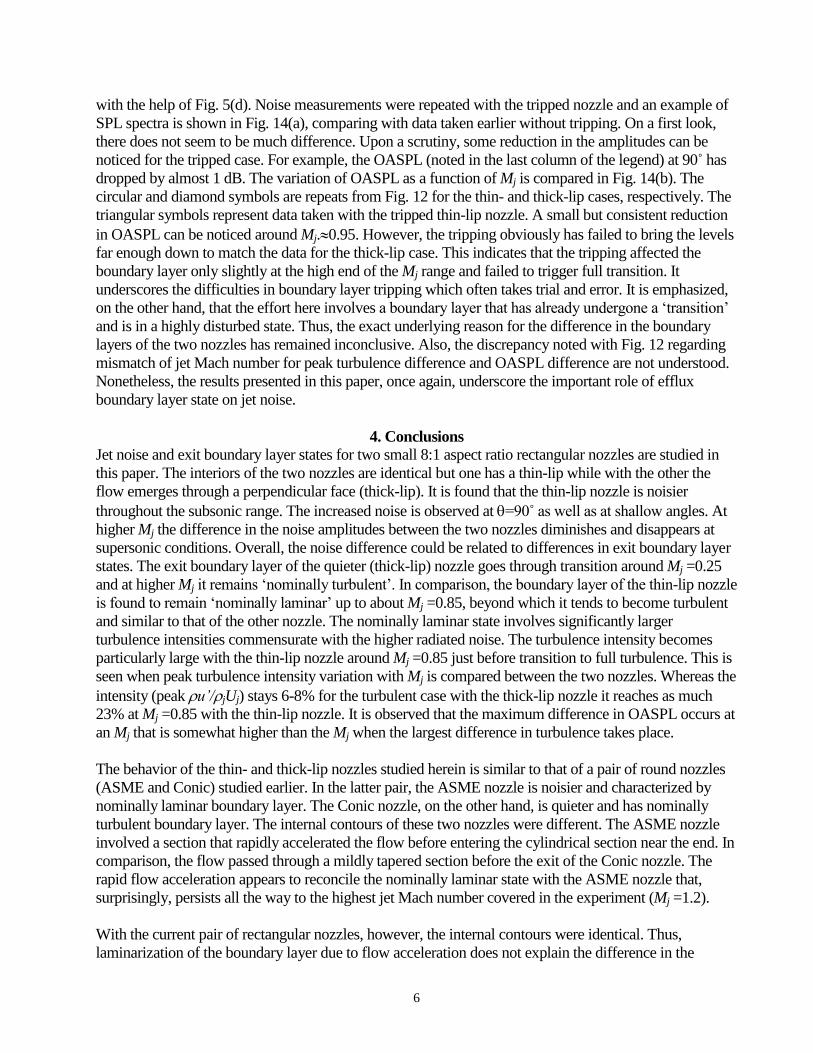
Fig. 1 Internal contours of two round nozzles investigated

in [9] and [10]. The radius r and axial distance x are

nondimensionalized by nozzle diameter (D) which was 2”

in [9] and 1” in [10].

(a)

(b)f (kHz)

SP

L(d

B)

100

101

65

70

75

80

85

90

asme =90 MJ= 1.002 104.66dB

conic =90 MJ= 1.001 103.34dB

Fig. 2 Comparison of SPL spectra at =90°for Conic and

ASME nozzles at Mj 1.0; (a) data from [9], (b) data

from [10].

Mj

ReD

x 10-3

2/D

0 0.2 0.4 0.6 0.8 1

0 200 400 600

0

0.002

0.004

0.006

conic

asme

Lam prediction (c=0.92)

Fig. 3 Exit boundary momentum thickness vs. Jet Mach

number for ASME and Conic nozzles; corresponding

scale for Reynolds number (based on nozzle diameter) is

shown at top.

t (ms)

u(f

t/s)

0 100 200 300 400 500

600

800

1000

1200

1400ASME

0.572

0.935

Mj=1.116

0.755

t (ms)

u(f

t/s)

0 100 200 300 400 500

600

800

1000

1200

1400CONIC

0.572

0.935

Mj=1.116

0.755

t (ms)

u(f

t/s)

0 100 200 300 400 500

100

200

300

400

500ASME

0.088

0.134

0.193

0.271

0.333

Mj=0.434

t (ms)

u(f

t/s)

0 100 200 300 400 500

100

200

300

400

500CONIC

0.088

0.134

0.193

0.271

0.333

Mj=0.434

Fig. 4 Velocity traces measured on the high speed edge of

the boundary layer (at approximately 0.9Uj – point) for

the ASME nozzle (left) and the Conic nozzle (right), at

indicated values of Mj.

10

(a)

(b)

(c)

(d)

Fig. 5 Experimental facility. (a) two rectangular nozzles

of aspect ratio 8:1; thin-lip case on left and thick-lip case

on right, (b) thin-lip nozzle with hot-wire in exit boundary

layer, (c) thin-lip nozzle with flange, (d) thin-lip nozzle

with boundary layer trip.

(a)f (kHz)

SP

L(d

B)

SP

L(d

B)

100

101

50

60

70

80

90

60

70

80

90

100

Tk-mn =25 MJ= 0.961 101.12dB

Tk-mn =90 MJ= 0.961 95.29dB

Tn-mn =25 MJ= 0.960 104.66dB

Tn-mn =90 MJ= 0.960 100.09dB

<=

=>

(b)f (kHz)

SP

L(d

B)

SP

L(d

B)

100

101

50

60

70

80

90

60

70

80

90

100

Tk-mj =25 MJ= 0.960 100.48dB

Tk-mj =90 MJ= 0.960 96.34dB

Tn-mj =25 MJ= 0.959 104.25dB

Tn-mj =90 MJ= 0.959 100.54dB

<=

=>

Fig. 6 Comparison of SPL spectra at Mj 0.96; (a) on

minor axis, (b) on major axis. In each figure, upper pair of

curves for =25 (scale on left), lower pair of curves for

= 90 (scale on right). Solid (red) curves are for thin-lip

case and dashed (blue) curves are for thick-lip case.

11

(a)

(b)

(c)f (kHz)

SP

L(d

B)

SP

L(d

B)

100

101

50

60

70

80

90

60

70

80

90

100

Tk-mn =25 MJ= 1.005 102.76dB

Tk-mn =90 MJ= 1.005 96.62dB

Tn-mn =25 MJ= 1.008 104.93dB

Tn-mn =90 MJ= 1.008 99.33dB

<=

=>

(d)

Fig. 7 Comparison of SPL spectra for the two rectangular

nozzles shown in the same format as in Fig. 6 at four

other jet Mach numbers: (a) Mj=0.796, (b) Mj=0.889, (c)

Mj=1.005, (d) Mj=1.048.

t (ms)

u(f

t/s)

0 100 200 300 400 500

600

800

1000

1200R8TN

0.572

0.920

Mj=1.116

0.755

t (ms)

u(f

t/s)

0 100 200 300 400 500

600

800

1000

1200R8TK

0.572

0.920

Mj=1.116

0.755

t (ms)

u(f

t/s)

0 100 200 300 400 500

100

200

300

400

500R8TN

0.088

0.134

0.193

0.271

0.333

Mj=0.434

t (ms)

u(f

t/s)

0 100 200 300 400 500

100

200

300

400

500R8TK

0.088

0.134

0.193

0.271

0.333

Mj=0.434

Fig. 8 Velocity traces as in Fig. 4 (at approximately 0.9Uj

– point) for the thin-lip nozzle (left) and the thick-lip

nozzle (right), at indicated values of Mj.

f (kHz)

SP

L(d

B)

SP

L(d

B)

100

101

40

50

60

70

80

90

100

60

70

80

90

100

Tk-mn =25 MJ= 1.048 105.29dB

Tk-mn =90 MJ= 1.048 97.81dB

Tn-mn =25 MJ= 1.047 104.99dB

Tn-mn =90 MJ= 1.047 98.83dB

<=

=>

f (kHz)

SP

L(d

B)

SP

L(d

B)

100

101

40

50

60

70

80

50

60

70

80

90

Tk-mn =25 MJ= 0.889 98.57dB

Tk-mn =90 MJ= 0.889 93.12dB

Tn-mn =25 MJ= 0.889 100.50dB

Tn-mn =90 MJ= 0.889 96.13dB

<=

=>

f (kHz)

SP

L(d

B)

SP

L(d

B)

100

101

40

50

60

70

80

50

60

70

80

90

Tk-mn =25 MJ= 0.796 94.58dB

Tk-mn =90 MJ= 0.796 89.99dB

Tn-mn =25 MJ= 0.798 96.59dB

Tn-mn =90 MJ= 0.798 92.71dB

<=

=>

12

(a)(y-y

w)/D

U

/jU

j

u

'/

jUj

-0.08 -0.06 -0.04 -0.02 00

0.2

0.4

0.6

0.8

1

0

0.04

0.08

0.12

R8TK U

R8TN U

R8TK u'

R8TN u'

Mj= 0.186

(b)(y-y

w)/D

U

/jU

j

u

'/

jUj

-0.08 -0.06 -0.04 -0.02 00

0.2

0.4

0.6

0.8

1

0

0.04

0.08

0.12

R8TK U

R8TN U

R8TK u'

R8TN u'

Mj= 0.574

(c)(y-y

w)/D

U

/jU

j

u

'/

jUj

-0.08 -0.06 -0.04 -0.02 00

0.2

0.4

0.6

0.8

1

0

0.08

0.16

0.24

R8TK U

R8TN U

R8TK u'

R8TN u'

Mj= 0.837

(d)(y-y

w)/D

U

/jU

j

u

'/

jUj

-0.08 -0.06 -0.04 -0.02 00

0.2

0.4

0.6

0.8

1

0

0.04

0.08

0.12

R8TK U

R8TN U

R8TK u'

R8TN u'

Mj= 1.032

Fig. 9 Comparison of boundary layer velocity profiles

measured 0.030 inch from the exit on the middle of the

long edge (R8TK=thick-lip case, R8TN=thin-lip case). In

each figure, curves without symbols are for mean velocity

(scale on left) and curves with symbols for turbulence

intensity (scale on right): (a) Mj=0.186, (b) Mj=0.574, (c)

Mj=0.837, (d) Mj=1.032.

Mj

ReD

x 10-3

2/D

0 0.2 0.4 0.6 0.8 1 1.2

0 100 200 300 400

0

0.002

0.004

0.006

0.008

R8TN

R8TK

Lam prediction(c=0.92)

Fig. 10 Exit boundary layer momentum thickness vs. Mj

for thin-lip (R8TN) and thick-lip (R8TK) nozzles;

corresponding scale for jet Reynolds number shown at

top.

Mj

ReD

x 10-3

u

' ma

x/

jUj

0 0.2 0.4 0.6 0.8 1 1.2

0 100 200 300 400

0.05

0.1

0.15

0.2

0.25

R8TN

R8TK

Fig. 11 Variation of peak turbulence intensity in the

boundary layer corresponding to the data of Fig. 10.

13

Fig. 12 Variation of OASPL with Mj (open symbols; scale

on left). Triangular data points for thin-lip nozzle with

hot-wire in boundary layer (Fig. 5b). Also shown at top

are peak turbulence intensity data from Fig. 11 (solid

symbols; scale on right).

Fig. 13 Comparison of SPL spectra for the thin-lip nozzle

with and without flange (Fig. 5c), shown in same format

as in Fig. 6; Mj0.96. Solid lines: flange case, dotted lines:

no-flange case.

(a)

(b)

Fig. 14 Effect of boundary layer trip on noise from the

thin-lip nozzle: (a) comparison of SPL spectra (in same

format as in Fig. 6), (b) comparison of OASPL vs. Mj

(circular and diamond data points repeated from Fig.12);

triangular data points for tripped boundary layer (Fig. 5d).

Mj

OA

SP

L(d

B)

0.4 0.6 0.8 1 1.2

80

90

100

110

R8TN oaspl =90o

R8TK oaspl =90o

R8TN oaspl BL trip

f (kHz)

SP

L(d

B)

SP

L(d

B)

100

101

50

60

70

80

90

60

70

80

90

100

R8TN =25 MJ= 0.961 104.73dB

R8TN =90 MJ= 0.961 100.15dB

BL trip =25 MJ= 0.961 104.17dB

BL trip =90 MJ= 0.961 99.17dB

<=

=>

f (kHz)

SP

L(d

B)

SP

L(d

B)

100

101

50

60

70

80

90

60

70

80

90

100

R8TN =25 MJ= 0.961 104.73dB

R8TN =90 MJ= 0.961 100.15dB

R8TN-F =25 MJ= 0.963 105.09dB

R8TN-F =90 MJ= 0.963 100.23dB

<=

=>

Mj

OA

SP

L(d

B)

u' m

ax

/U

j

0.4 0.6 0.8 1 1.2

80

90

100

110

0

R8TN u'max

R8TK u'max

R8TN oaspl =90o

R8TK oaspl =90o

R8TN oaspl hw in

0.25