Embed Size (px)
Citation preview
1/21
EECE 301 Signals & SystemsProf. Mark Fowler
Note Set #13• C-T Signals: Fourier Series (for Periodic Signals)• Reading Assignment: Section 3.2 & 3.3 of Kamen and Heck
2/21
Ch. 1 IntroC-T Signal Model
Functions on Real Line
D-T Signal ModelFunctions on Integers
System PropertiesLTI
CausalEtc
Ch. 2 Diff EqsC-T System Model
Differential EquationsD-T Signal Model
Difference Equations
Zero-State Response
Zero-Input ResponseCharacteristic Eq.
Ch. 2 Convolution
C-T System ModelConvolution Integral
D-T System ModelConvolution Sum
Ch. 3: CT Fourier Signal Models
Fourier SeriesPeriodic Signals
Fourier Transform (CTFT)Non-Periodic Signals
New System Model
New SignalModels
Ch. 5: CT Fourier System Models
Frequency ResponseBased on Fourier Transform
New System Model
Ch. 4: DT Fourier Signal Models
DTFT(for “Hand” Analysis)
DFT & FFT(for Computer Analysis)
New SignalModel
Powerful Analysis Tool
Ch. 6 & 8: Laplace Models for CT
Signals & Systems
Transfer Function
New System Model
Ch. 7: Z Trans.Models for DT
Signals & Systems
Transfer Function
New SystemModel
Ch. 5: DT Fourier System Models
Freq. Response for DTBased on DTFT
New System Model
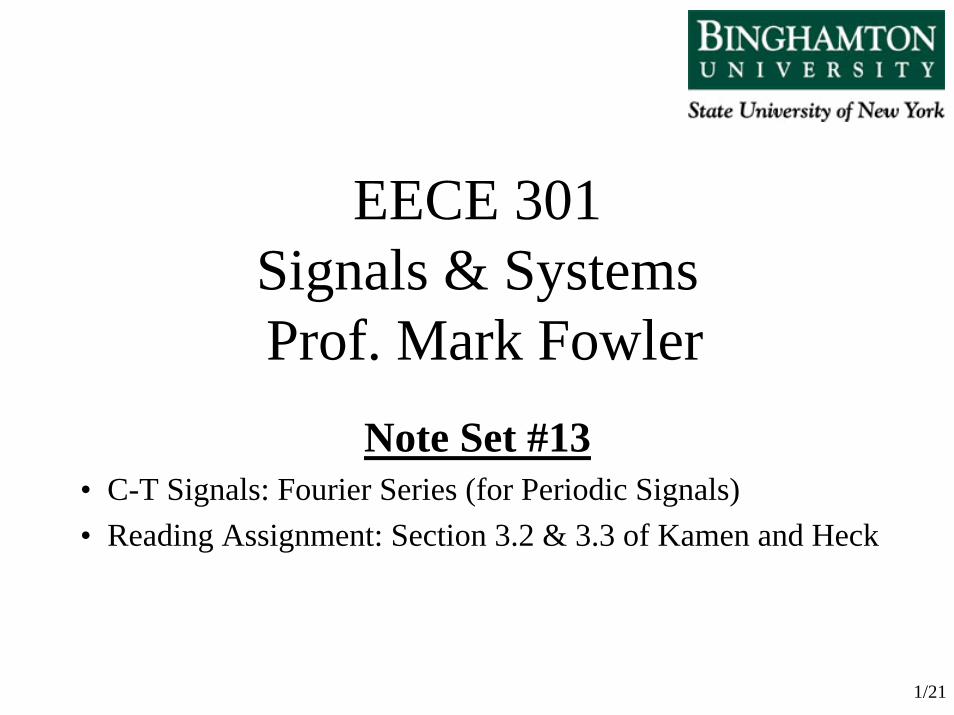
Course Flow DiagramThe arrows here show conceptual flow between ideas. Note the parallel structure between
the pink blocks (C-T Freq. Analysis) and the blue blocks (D-T Freq. Analysis).
3/21
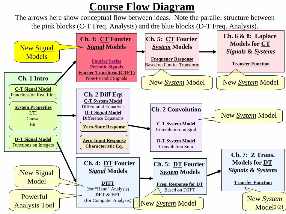
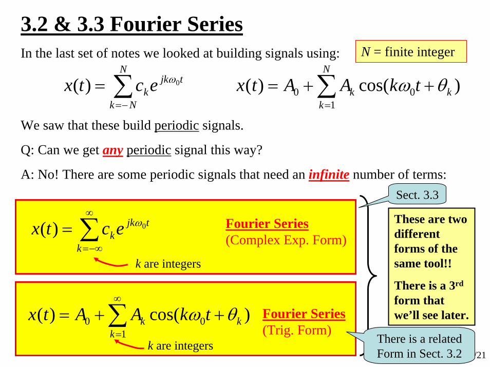
3.2 & 3.3 Fourier SeriesIn the last set of notes we looked at building signals using:
∑−=
=N
Nk
tjkkectx 0)( ω
N = finite integer
We saw that these build periodic signals.
Q: Can we get any periodic signal this way?
A: No! There are some periodic signals that need an infinite number of terms:
∑=
++=N
kkk tkAAtx
100 )cos()( θω
∑∞
−∞=
=k
tjkkectx 0)( ω Fourier Series
(Complex Exp. Form)
k are integers
∑∞
=
++=1
00 )cos()(k
kk tkAAtx θω
k are integers
Fourier Series(Trig. Form)
These are two different forms of the same tool!!
There is a 3rd
form that we’ll see later.
Sect. 3.3
There is a related Form in Sect. 3.2
4/21
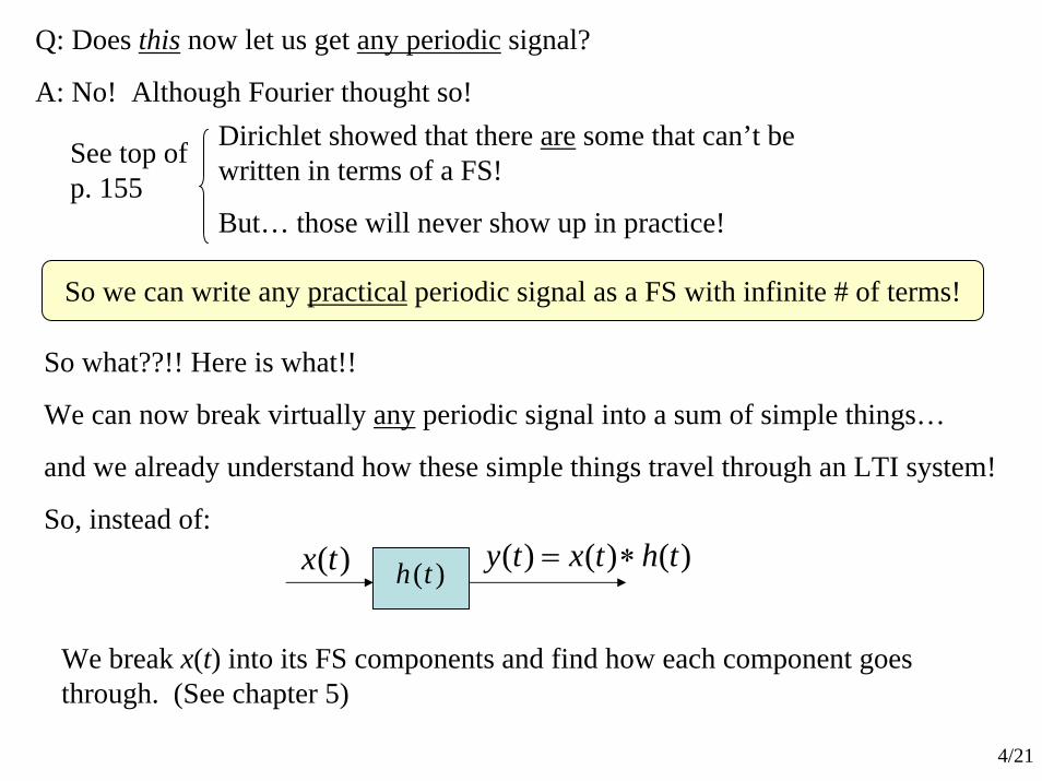
Q: Does this now let us get any periodic signal?
A: No! Although Fourier thought so!Dirichlet showed that there are some that can’t be written in terms of a FS!
But… those will never show up in practice!
See top of p. 155
So we can write any practical periodic signal as a FS with infinite # of terms!
So what??!! Here is what!!
We can now break virtually any periodic signal into a sum of simple things…
and we already understand how these simple things travel through an LTI system!
So, instead of:
)(th)(tx )()()( thtxty ∗=
We break x(t) into its FS components and find how each component goes through. (See chapter 5)
5/21
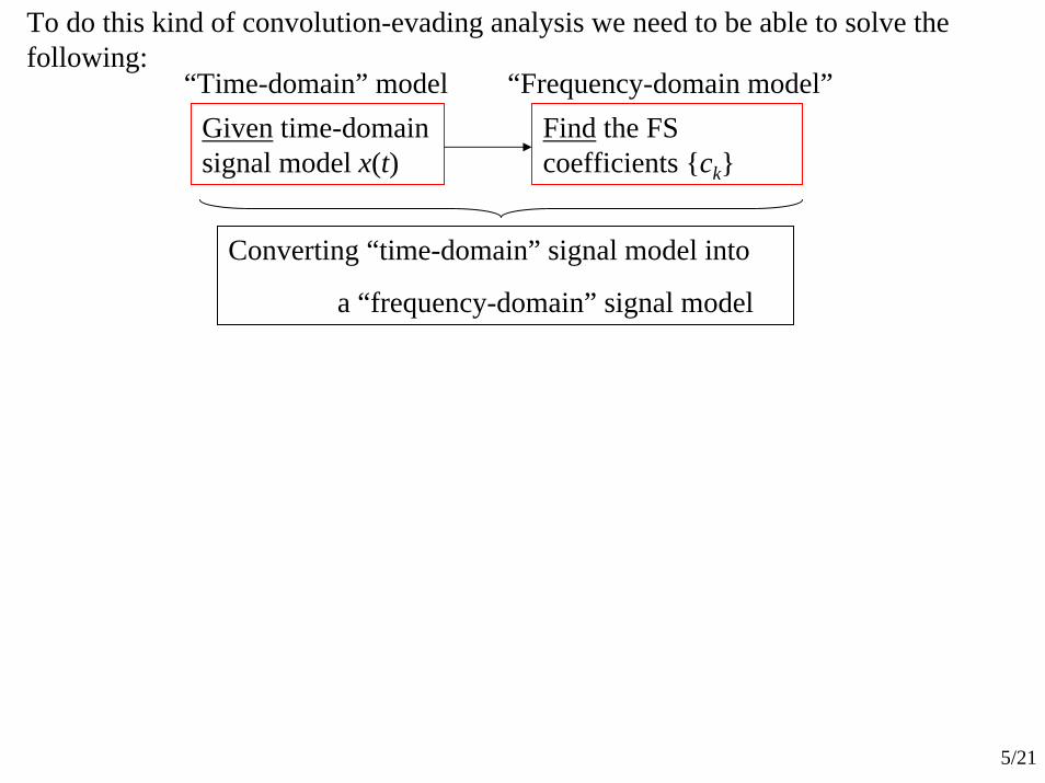
To do this kind of convolution-evading analysis we need to be able to solve the following:
Given time-domain signal model x(t)
Find the FS coefficients {ck}
“Time-domain” model “Frequency-domain model”
Converting “time-domain” signal model into
a “frequency-domain” signal model
6/21
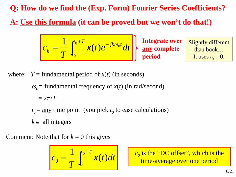
Q: How do we find the (Exp. Form) Fourier Series Coefficients?
A: Use this formula (it can be proved but we won’t do that!)
∫+ −=
Tt
t
tjkk dtetx
Tc 0
0
0)(1 ω Slightly different than book…It uses t0 = 0.
Integrate over any complete period
where: T = fundamental period of x(t) (in seconds)
ω0= fundamental frequency of x(t) (in rad/second)
= 2π/T
t0 = any time point (you pick t0 to ease calculations)
k ∈ all integers
Comment: Note that for k = 0 this gives
∫+
=Tt
tdttx
Tc 0
0
)(10
c0 is the “DC offset”, which is the time-average over one period
7/21
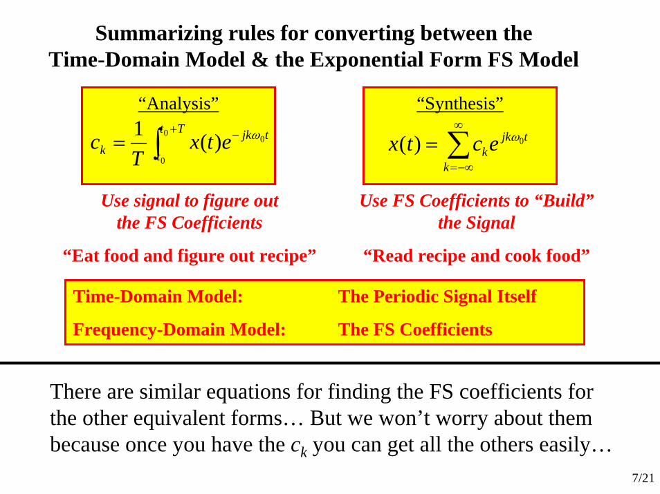
Summarizing rules for converting between the Time-Domain Model & the Exponential Form FS Model
“Synthesis”
∑∞
−∞=
=k
tjkkectx 0)( ω
Use FS Coefficients to “Build”the Signal
“Read recipe and cook food”
“Analysis”
∫+ −=
Tt
t
tjkk etx
Tc 0
0
0)(1 ω
Use signal to figure out the FS Coefficients
“Eat food and figure out recipe”
Time-Domain Model: The Periodic Signal Itself
Frequency-Domain Model: The FS Coefficients
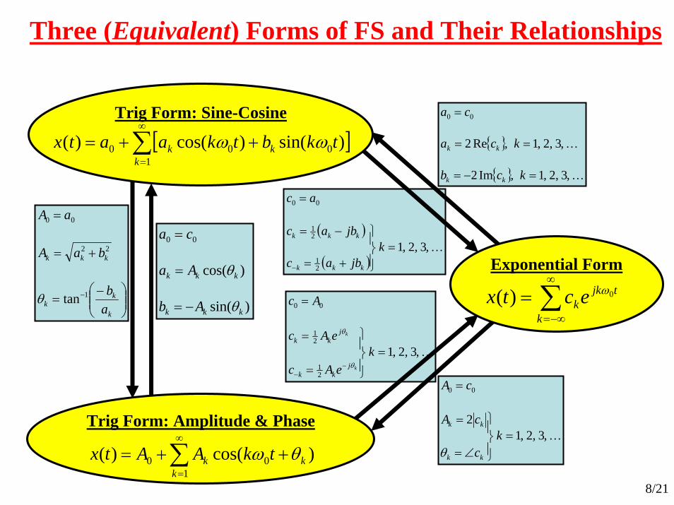
There are similar equations for finding the FS coefficients for the other equivalent forms… But we won’t worry about them because once you have the ck you can get all the others easily…
8/21
…,3,2,1
21
21
00
=⎪⎭
⎪⎬⎫
=
=
=
−−
keAc
eAc
Ac
k
k
jkk
jkk
θ
θ
( )
( )…,3,2,1
21
21
00
=⎪⎭
⎪⎬⎫
+=
−=
=
−
kjbac
jbac
ac
kkk
kkk
Exponential Form
∑∞
−∞=
=k
tjkkectx 0)( ω
Trig Form: Amplitude & Phase
∑∞
=
++=1
00 )cos()(k
kk tkAAtx θω
Trig Form: Sine-Cosine
[ ]∑∞
=
++=1
000 )sin()cos()(k
kk tkbtkaatx ωω { }
{ } …
…
,3,2,1,Im2
,3,2,1,Re2
00
=−=
==
=
kcb
kca
ca
kk
kk
…,3,2,12
00
=⎪⎭
⎪⎬⎫
∠=
=
=
kc
cA
cA
kk
kk
θ
⎟⎟⎠
⎞⎜⎜⎝
⎛ −=
+=
=
−
k
kk
kkk
ab
baA
aA
1
22
00
tanθ )sin(
)cos(
00
kkk
kkk
Ab
Aa
ca
θ
θ
−=
=
=
Three (Equivalent) Forms of FS and Their Relationships
9/21
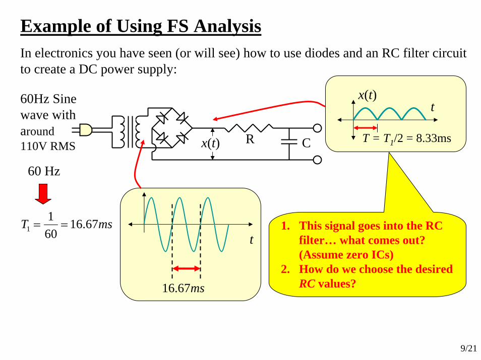
Example of Using FS AnalysisIn electronics you have seen (or will see) how to use diodes and an RC filter circuit to create a DC power supply:
60Hz Sine wave with around 110V RMS
msT 67.16601
1 ==
x(t) R C
60 Hz
t
ms67.16
x(t)
T = T1/2 = 8.33ms
t
1. This signal goes into the RC filter… what comes out? (Assume zero ICs)
2. How do we choose the desired RC values?
10/21
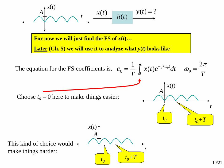
t )(th)(tx ?)(x(t)
=tyA
For now we will just find the FS of x(t)…
Later (Ch. 5) we will use it to analyze what y(t) looks like
The equation for the FS coefficients is: ∫ −=T tjk
k dtetxT
c0
0)(1 ω
Tπω 2
0 =
Choose t0 = 0 here to make things easier:t
x(t)A
t0 t0+T
This kind of choice would make things harder: t
x(t)A
t0t0+T
11/21
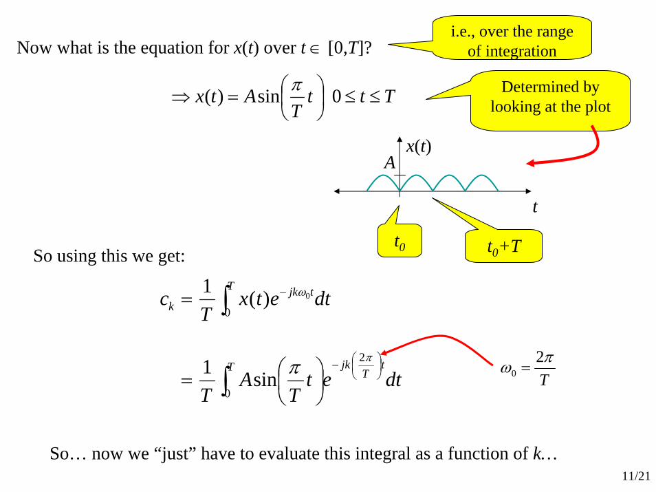
Now what is the equation for x(t) over t ∈ [0,T]?
TttT
Atx ≤≤⎟⎠⎞
⎜⎝⎛=⇒ 0sin)( π
So using this we get:
∫
∫
⎟⎠⎞
⎜⎝⎛−
−
⎟⎠⎞
⎜⎝⎛=
=
T tT
jk
T tjkk
dtetT
AT
dtetxT
c
0
2
0
sin1
)(10
π
ω
πTπω 2
0 =
i.e., over the range of integration
Determined by looking at the plot
t
x(t)A
t0 t0+T
So… now we “just” have to evaluate this integral as a function of k…
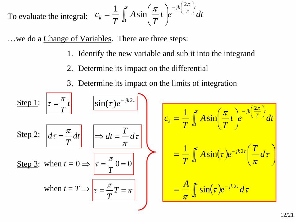
12/21
…we do a Change of Variables. There are three steps:
1. Identify the new variable and sub it into the integrand
2. Determine its impact on the differential
3. Determine its impact on the limits of integration
∫⎟⎠⎞
⎜⎝⎛−
⎟⎠⎞
⎜⎝⎛=
T tT
jk
k dtetT
AT
c0
2
sin1 ππTo evaluate the integral:
dtT
d πτ = τπ
dTdt =⇒Step 2:
when t = 0 ⇒
when t = T ⇒
Step 3: 00 ==Tπτ
ππτ == TT
tTπτ =Step 1: ττ 2)sin( jke−
( )
( )∫
∫
∫
−
−
⎟⎠⎞
⎜⎝⎛−
=
⎟⎠⎞
⎜⎝⎛=
⎟⎠⎞
⎜⎝⎛=
π τ
π τ
π
ττπ
τπ
τ
π
0
2
0
2
0
2
sin
sin1
sin1
deA
dTeAT
dtetT
AT
c
jk
jk
T tT
jk
k
13/21
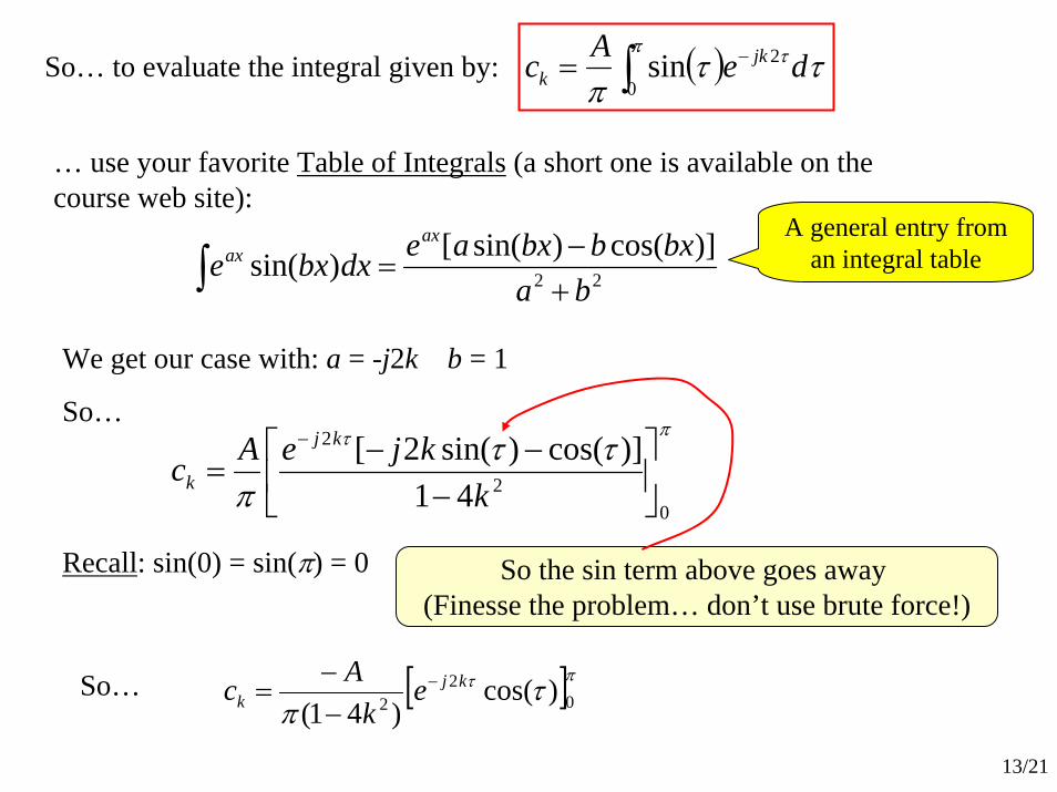
… use your favorite Table of Integrals (a short one is available on the course web site):
∫ +−
= 22
)]cos()sin([)sin(ba
bxbbxaedxbxeax
ax
We get our case with: a = -j2k b = 1
So…πτ ττ
π 02
2
41)]cos()sin(2[⎥⎦
⎤⎢⎣
⎡−
−−=
−
kkjeAc
kj
k
So… [ ]πτ τπ 0
22 )cos()41(
kjk e
kAc −
−−
=
Recall: sin(0) = sin(π) = 0 So the sin term above goes away (Finesse the problem… don’t use brute force!)
( )∫ −=π τ ττ
π 0
2sin deAc jkkSo… to evaluate the integral given by:
A general entry from an integral table
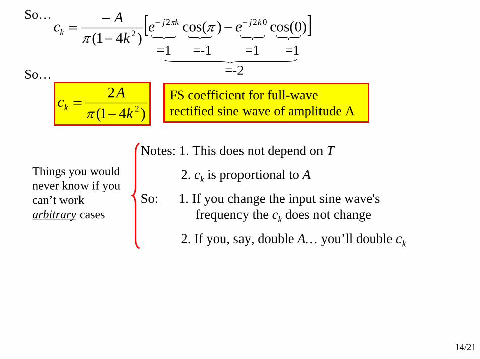
14/21
So… [ ])0cos()cos()41(
0222
kjkjk ee
kAc −− −
−−
= ππ
π
=1 =1=-1 =1=-2So…
)41(2
2kAck −
=π
FS coefficient for full-wave rectified sine wave of amplitude A
Notes: 1. This does not depend on T
2. ck is proportional to A
So: 1. If you change the input sine wave's frequency the ck does not change
2. If you, say, double A… you’ll double ck
Things you would never know if you can’t work arbitrary cases
15/21
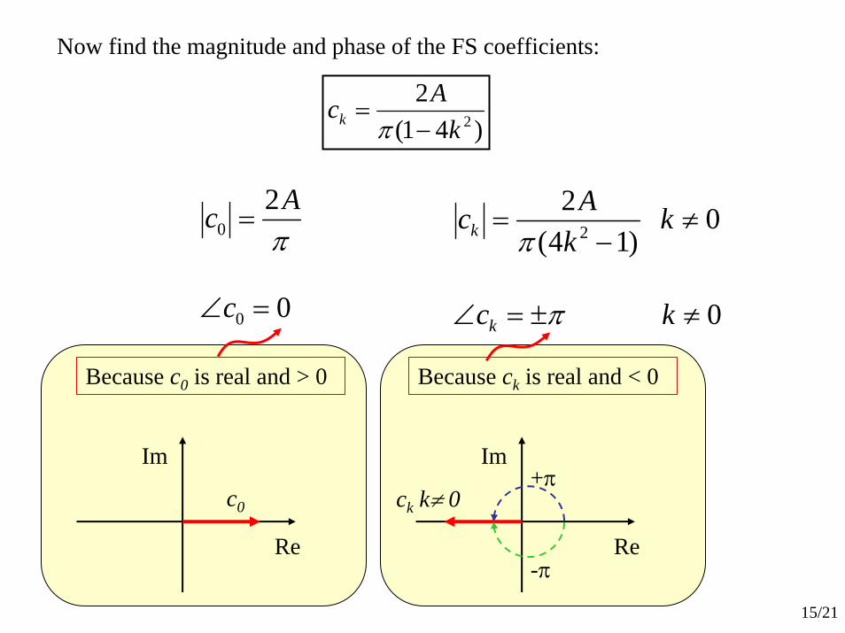
Re
Im
ck k≠ 0
0
2
0
0
=∠
=
c
Acπ
0
0)14(
22
≠±=∠
≠−
=
kc
kk
Ac
k
k
π
π
Because c0 is real and > 0 Because ck is real and < 0
Now find the magnitude and phase of the FS coefficients:
)41(2
2kAck −
=π
Re
Im
c0
+π
-π
16/21
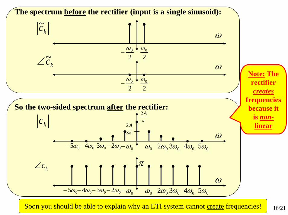
So the two-sided spectrum after the rectifier:πA2
π32A
ω0ω 02ω 03ω 04ω 05ω0ω−02ω−03ω−04ω−05ω−
ω0ω 02ω 03ω 04ω 05ω0ω−02ω−03ω−04ω−05ω−
kc
kc∠ π
The spectrum before the rectifier (input is a single sinusoid):
20ω
20ω−
ω
20ω
20ω−
ω
kc~
kc~∠Note: The rectifier creates
frequencies because it
is non-linear
Soon you should be able to explain why an LTI system cannot create frequencies!

17/21
The rectified sine wave has Trig. Form FS: ∑∞
=
+−
+=1
02 )cos()14(
42)(k
tkk
AAtx πωππ
Ak θkA0
Now you can find the Trigonometric form of FSOnce you have the ck for the Exp. Form, Euler’s formula gives the Trig Form as:
∑∞
=
∠++=1
00 )cos(2)(k
kk ctkcctx ω General Result!!
So… the input to the RC circuit consists of a superposition of sinusoids… and you know from circuits class how to:
1. Handle a superposition of inputs to an RC circuit
2. Determine how a single sinusoid of a given frequency goes through an RC circuit
πA2
π34A
ω0ω 02ω 03ω 04ω 05ω
The one-sided spectrum is:
ω0ω 02ω 03ω 04ω 05ω
π …
…Magnitude Spectrum
Phase Spectrum
Ak
θk
18/21
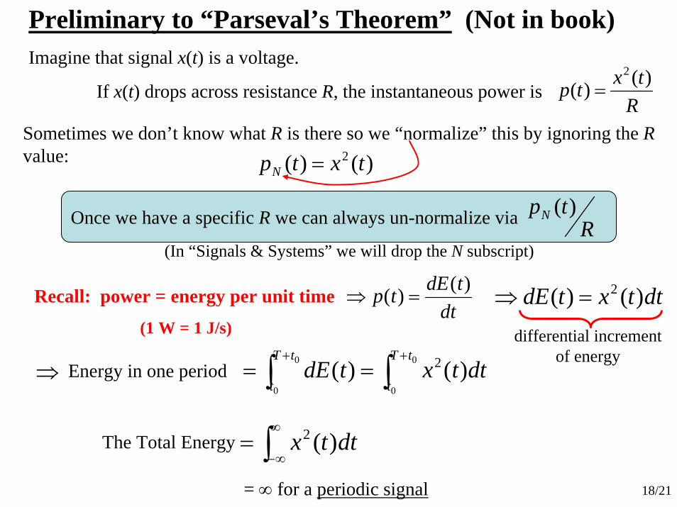
Preliminary to “Parseval’s Theorem” (Not in book)Imagine that signal x(t) is a voltage.
If x(t) drops across resistance R, the instantaneous power is R
txtp )()(2
=
Sometimes we don’t know what R is there so we “normalize” this by ignoring the Rvalue: )()( 2 txtpN =
⇒ Energy in one period ∫∫++
==0
0
0
0
)()( 2tT
t
tT
tdttxtdE
Recall: power = energy per unit time
(1 W = 1 J/s)dt
tdEtp )()( =⇒ dttxtdE )()( 2=⇒
differential increment of energy
Once we have a specific R we can always un-normalize via RtpN )(
(In “Signals & Systems” we will drop the N subscript)
The Total Energy ∫∞
∞−= dttx )(2
= ∞ for a periodic signal
19/21
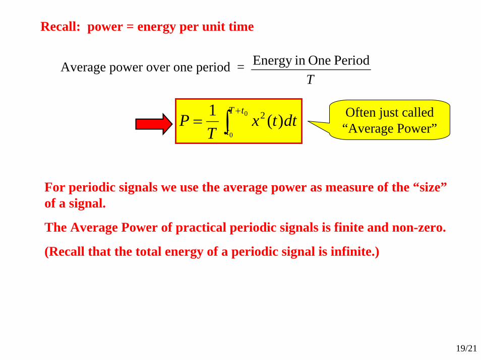
∫+
= 0
0
)(1 2tT
tdttx
TP
Average power over one period =T
PeriodOne inEnergy
Recall: power = energy per unit time
For periodic signals we use the average power as measure of the “size”of a signal.
The Average Power of practical periodic signals is finite and non-zero.
(Recall that the total energy of a periodic signal is infinite.)
Often just called “Average Power”
20/21
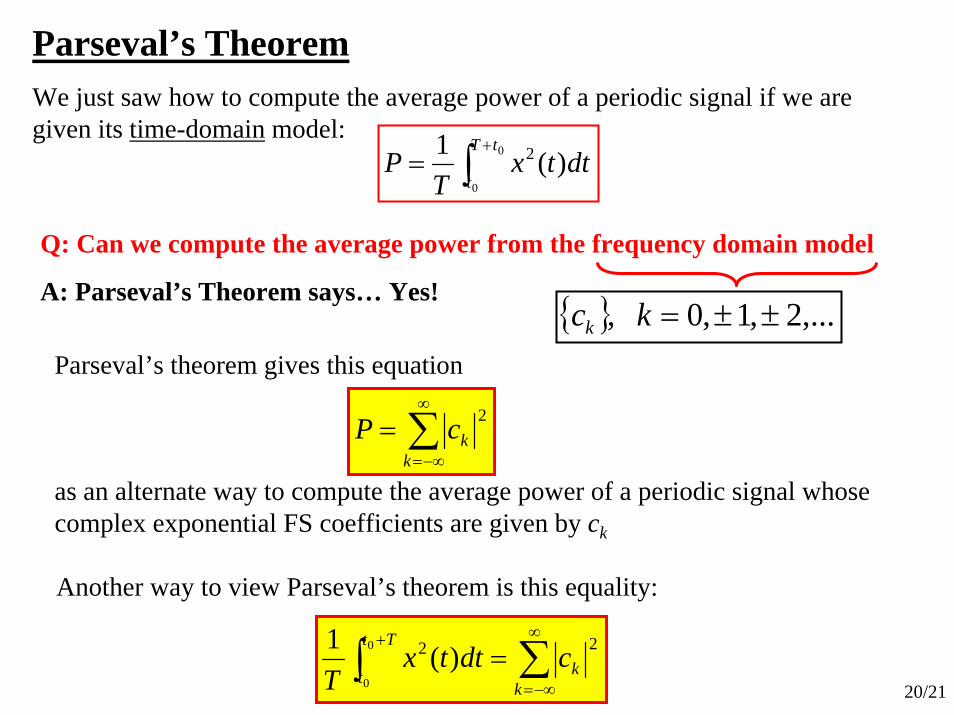
Parseval’s TheoremWe just saw how to compute the average power of a periodic signal if we are given its time-domain model:
∫+
= 0
0
)(1 2tT
tdttx
TP
Q: Can we compute the average power from the frequency domain model
A: Parseval’s Theorem says… Yes! { } ,...2,1,0, ±±=kck
∑∞
−∞=
=k
kcP 2
Another way to view Parseval’s theorem is this equality:
∑∫∞
−∞=
+=
kk
Tt
tcdttx
T220
0
)(1
Parseval’s theorem gives this equation
as an alternate way to compute the average power of a periodic signal whose complex exponential FS coefficients are given by ck
21/21
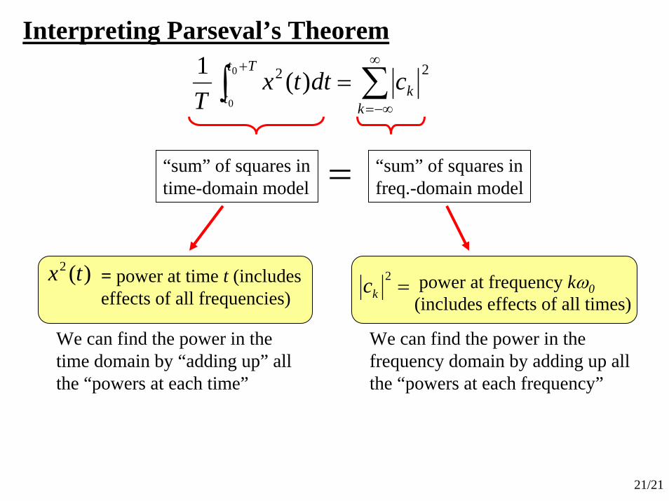
∑∫∞
−∞=
+=
kk
Tt
tcdttx
T220
0
)(1
“sum” of squares in time-domain model
“sum” of squares in freq.-domain model=
Interpreting Parseval’s Theorem
)(2 tx = power at time t (includes effects of all frequencies)
We can find the power in the time domain by “adding up” all the “powers at each time”
=2kc power at frequency kω0
(includes effects of all times)
We can find the power in the frequency domain by adding up all the “powers at each frequency”