Embed Size (px)
Citation preview

EE 581 Power Systems Admittance Matrix: Direct and Iterative solutions, Sensitivity
Overview and HW # 9
Chapter 6.1
Chapter 6.2
Chapter 6.3
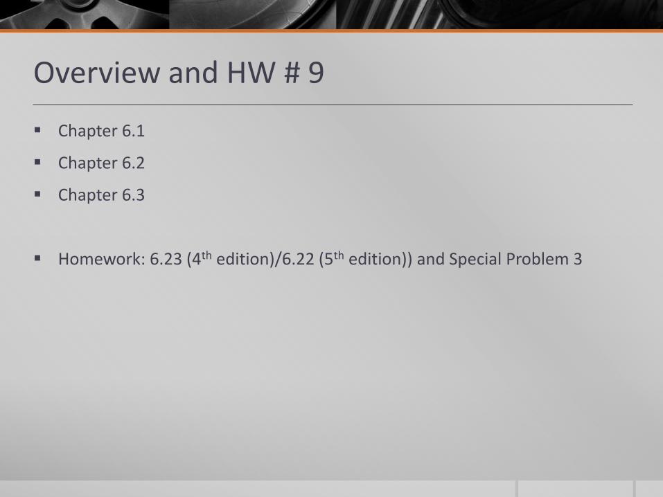
Homework: 6.23 (4th edition)/6.22 (5th edition)) and Special Problem 3
Overview and HW # 9
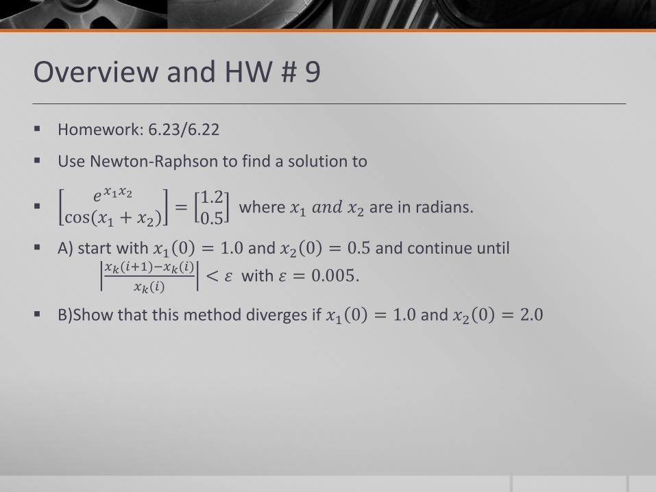
Homework: 6.23/6.22
Use Newton-Raphson to find a solution to
𝑒𝑥1𝑥2
cos(𝑥1 + 𝑥2)=
1.20.5
where 𝑥1𝑎𝑛𝑑𝑥2 are in radians.
A) start with 𝑥1 0 = 1.0 and 𝑥2 0 = 0.5 and continue until
𝑥𝑘(𝑖+1)−𝑥𝑘(𝑖)
𝑥𝑘(𝑖)< 𝜀 with 𝜀 = 0.005.
B)Show that this method diverges if 𝑥1 0 = 1.0 and 𝑥2 0 = 2.0
Overview and HW # 9
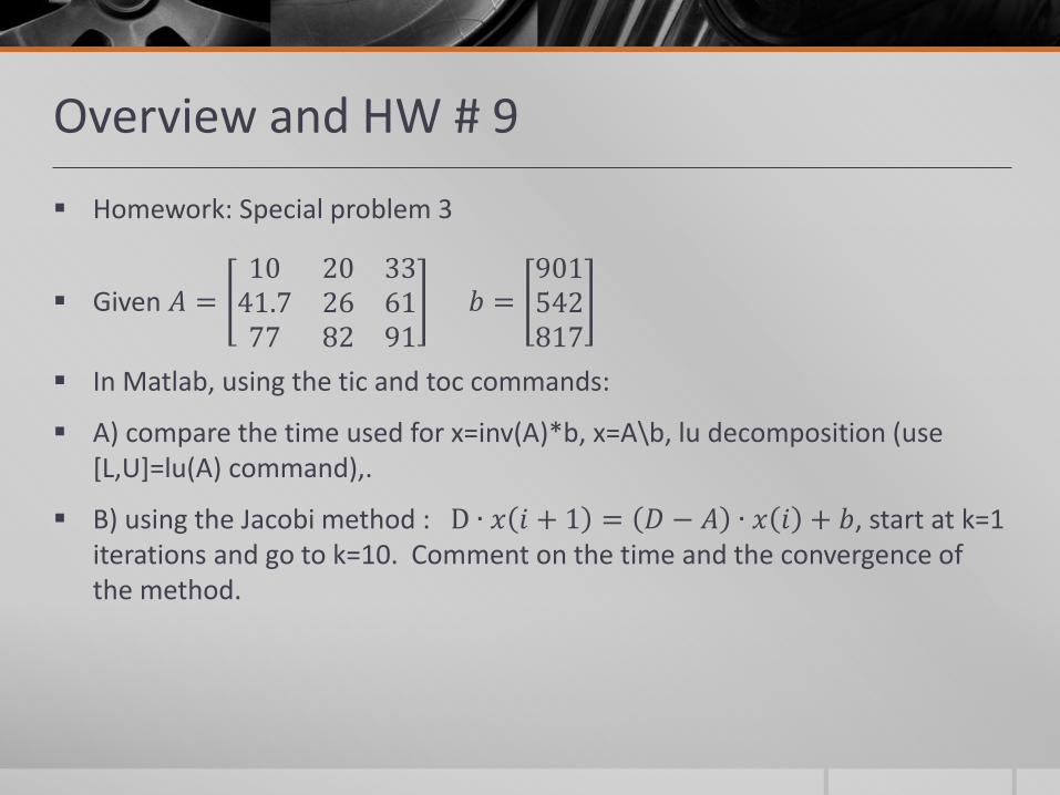
Homework: Special problem 3
Given 𝐴 =10 20 33
41.7 26 6177 82 91
𝑏 =901542817
In Matlab, using the tic and toc commands:
A) compare the time used for x=inv(A)*b, x=A\b, lu decomposition (use [L,U]=lu(A) command),.
B) using the Jacobi method : D ∙ 𝑥 𝑖 + 1 = 𝐷 − 𝐴 ∙ 𝑥 𝑖 + 𝑏, start at k=1 iterations and go to k=10. Comment on the time and the convergence of the method.
Overview and HW # 9
Homework: Special problem 3
A) check: 𝑥 =−41.577314.427231.1584
Chapter 6.1: Gaussian Elimination
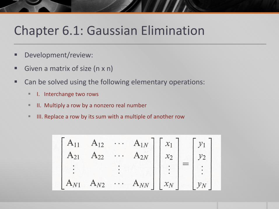
Development/review:
Given a matrix of size (n x n)
Can be solved using the following elementary operations:
I. Interchange two rows
II. Multiply a row by a nonzero real number
III. Replace a row by its sum with a multiple of another row
Chapter 6.1: Gaussian Elimination
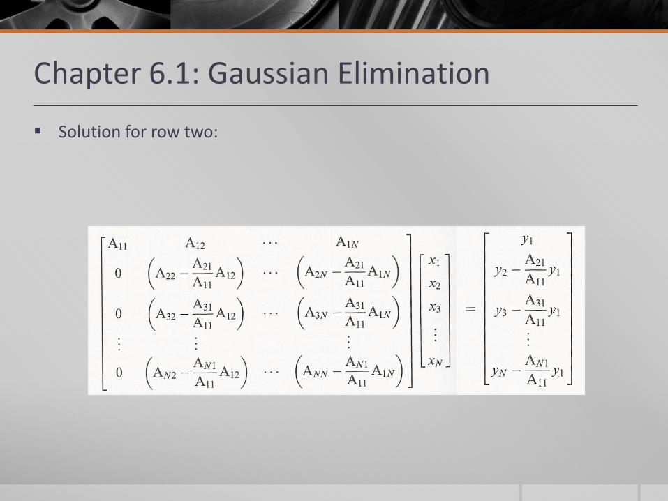
Solution for row two:
Chapter 6.1: Gaussian Elimination
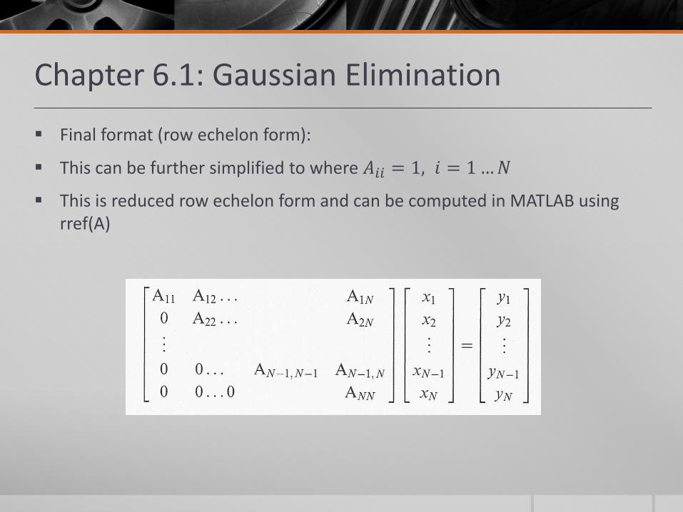
Final format (row echelon form):
This can be further simplified to where 𝐴𝑖𝑖 = 1, 𝑖 = 1…𝑁
This is reduced row echelon form and can be computed in MATLAB using rref(A)
Chapter 6.1: Gaussian Elimination
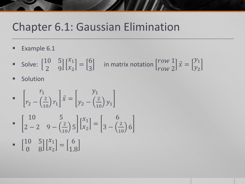
Example 6.1
Solve: 10 52 9
𝑥1
𝑥2=
63
in matrix notation 𝑟𝑜𝑤1𝑟𝑜𝑤2
𝑥 =𝑦1
𝑦2
Solution
𝑟1
𝑟2 −2
10𝑟1
𝑥 =𝑦1
𝑦2 −2
10𝑦1
10 5
2 − 2 9 −2
105
𝑥1
𝑥2=
6
3 −2
106
10 50 8
𝑥1
𝑥2=
61.8
Chapter 6.1: Gaussian Elimination
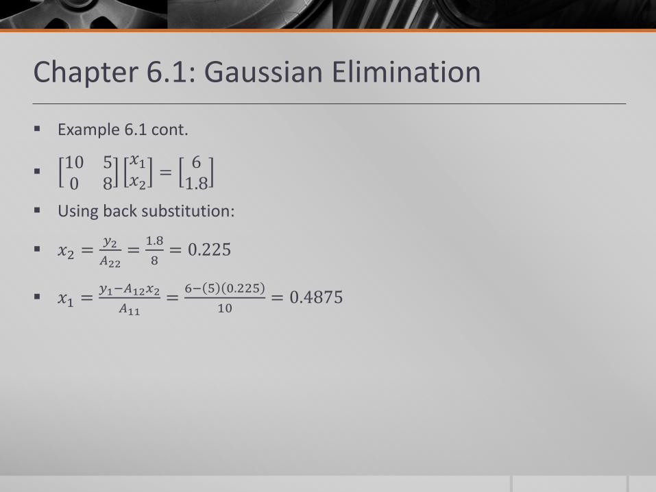
Example 6.1 cont.
10 50 8
𝑥1
𝑥2=
61.8
Using back substitution:
𝑥2 =𝑦2
𝐴22=
1.8
8= 0.225
𝑥1 =𝑦1−𝐴12𝑥2
𝐴11=
6− 5 0.225
10= 0.4875
Chapter 6.1: LU Decomposition
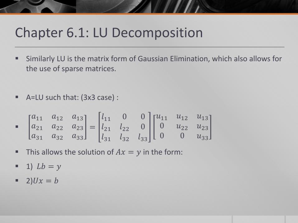
Similarly LU is the matrix form of Gaussian Elimination, which also allows for the use of sparse matrices.
A=LU such that: (3x3 case) :
𝑎11 𝑎12 𝑎13
𝑎21 𝑎22 𝑎23
𝑎31 𝑎32 𝑎33
=
𝑙11 0 0𝑙21 𝑙22 0𝑙31 𝑙32 𝑙33
𝑢11 𝑢12 𝑢13
0 𝑢22 𝑢23
0 0 𝑢33
This allows the solution of 𝐴𝑥 = 𝑦 in the form:
1) 𝐿𝑏 = 𝑦
2)𝑈𝑥 = 𝑏
Chapter 6.1: LU Decomposition
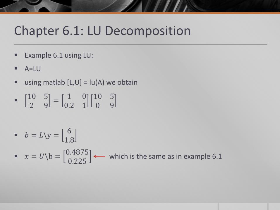
Example 6.1 using LU:
A=LU
using matlab [L,U] = lu(A) we obtain
10 52 9
=1 0
0.2 110 50 9
𝑏 = 𝐿\y =6
1.8
𝑥 = 𝑈\b =0.48750.225
which is the same as in example 6.1
Chapter 6.2: Jacobi and Gauss-Seidel
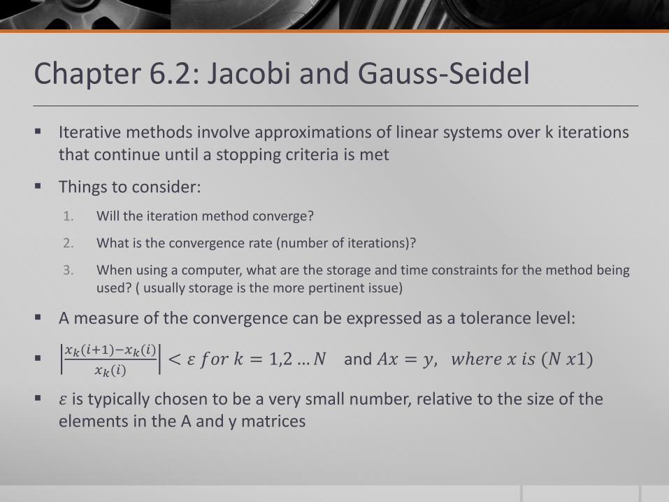
Iterative methods involve approximations of linear systems over k iterations that continue until a stopping criteria is met
Things to consider:
1. Will the iteration method converge?
2. What is the convergence rate (number of iterations)?
3. When using a computer, what are the storage and time constraints for the method being used? ( usually storage is the more pertinent issue)
A measure of the convergence can be expressed as a tolerance level:
𝑥𝑘(𝑖+1)−𝑥𝑘(𝑖)
𝑥𝑘(𝑖)< 𝜀𝑓𝑜𝑟𝑘 = 1,2…𝑁 and 𝐴𝑥 = 𝑦, 𝑤ℎ𝑒𝑟𝑒𝑥𝑖𝑠(𝑁𝑥1)
𝜀 is typically chosen to be a very small number, relative to the size of the elements in the A and y matrices
Chapter 6.2: Jacobi and Gauss-Seidel
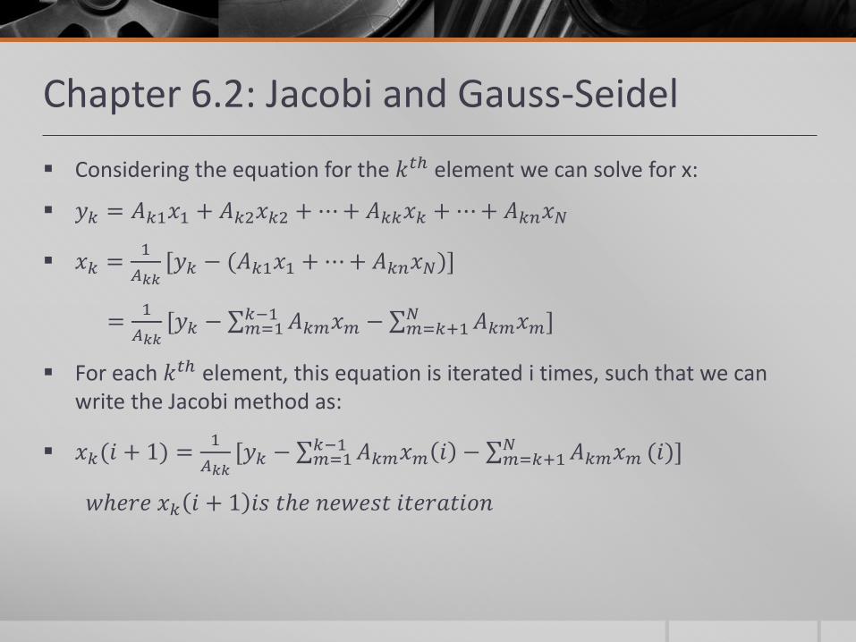
Considering the equation for the 𝑘𝑡ℎ element we can solve for x:
𝑦𝑘 = 𝐴𝑘1𝑥1 + 𝐴𝑘2𝑥𝑘2 + ⋯+ 𝐴𝑘𝑘𝑥𝑘 + ⋯+ 𝐴𝑘𝑛𝑥𝑁
𝑥𝑘 =1
𝐴𝑘𝑘[𝑦𝑘 − (𝐴𝑘1𝑥1 + ⋯+ 𝐴𝑘𝑛𝑥𝑁)]
=1
𝐴𝑘𝑘[𝑦𝑘 − 𝐴𝑘𝑚𝑥𝑚
𝑘−1𝑚=1 − 𝐴𝑘𝑚𝑥𝑚
𝑁𝑚=𝑘+1 ]
For each 𝑘𝑡ℎ element, this equation is iterated i times, such that we can write the Jacobi method as:
𝑥𝑘(𝑖 + 1) =1
𝐴𝑘𝑘[𝑦𝑘 − 𝐴𝑘𝑚𝑥𝑚 𝑖𝑘−1
𝑚=1 − 𝐴𝑘𝑚𝑥𝑚𝑁𝑚=𝑘+1 (𝑖)]
𝑤ℎ𝑒𝑟𝑒𝑥𝑘 𝑖 + 1 𝑖𝑠𝑡ℎ𝑒𝑛𝑒𝑤𝑒𝑠𝑡𝑖𝑡𝑒𝑟𝑎𝑡𝑖𝑜𝑛
Chapter 6.2: Jacobi and Gauss-Seidel
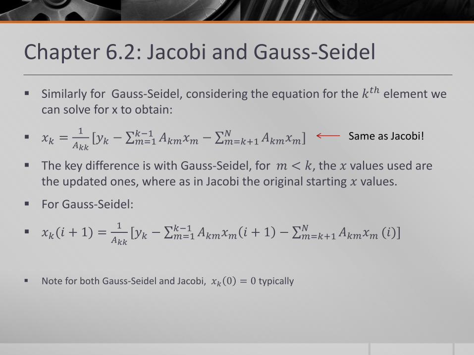
Similarly for Gauss-Seidel, considering the equation for the 𝑘𝑡ℎ element we can solve for x to obtain:
𝑥𝑘 =1
𝐴𝑘𝑘[𝑦𝑘 − 𝐴𝑘𝑚𝑥𝑚
𝑘−1𝑚=1 − 𝐴𝑘𝑚𝑥𝑚
𝑁𝑚=𝑘+1 ]
The key difference is with Gauss-Seidel, for 𝑚 < 𝑘, the 𝑥 values used are the updated ones, where as in Jacobi the original starting 𝑥 values.
For Gauss-Seidel:
𝑥𝑘(𝑖 + 1) =1
𝐴𝑘𝑘[𝑦𝑘 − 𝐴𝑘𝑚𝑥𝑚 𝑖 + 1𝑘−1
𝑚=1 − 𝐴𝑘𝑚𝑥𝑚𝑁𝑚=𝑘+1 (𝑖)]
Note for both Gauss-Seidel and Jacobi, 𝑥𝑘 0 = 0 typically
Same as Jacobi!
Chapter 6.2: Jacobi and Gauss-Seidel
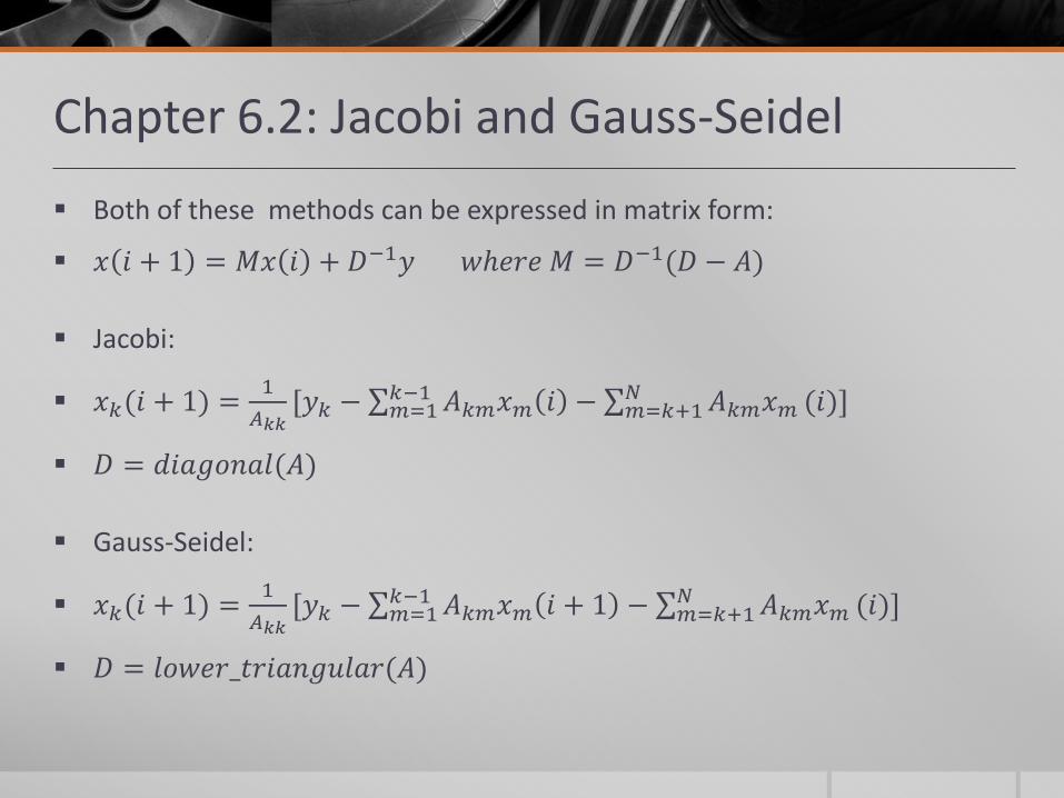
Both of these methods can be expressed in matrix form:
𝑥 𝑖 + 1 = 𝑀𝑥 𝑖 + 𝐷−1𝑦𝑤ℎ𝑒𝑟𝑒𝑀 = 𝐷−1(𝐷 − 𝐴)
Jacobi:
𝑥𝑘(𝑖 + 1) =1
𝐴𝑘𝑘[𝑦𝑘 − 𝐴𝑘𝑚𝑥𝑚 𝑖𝑘−1
𝑚=1 − 𝐴𝑘𝑚𝑥𝑚𝑁𝑚=𝑘+1 (𝑖)]
𝐷 = 𝑑𝑖𝑎𝑔𝑜𝑛𝑎𝑙(𝐴)
Gauss-Seidel:
𝑥𝑘(𝑖 + 1) =1
𝐴𝑘𝑘[𝑦𝑘 − 𝐴𝑘𝑚𝑥𝑚 𝑖 + 1𝑘−1
𝑚=1 − 𝐴𝑘𝑚𝑥𝑚𝑁𝑚=𝑘+1 (𝑖)]
𝐷 = 𝑙𝑜𝑤𝑒𝑟_𝑡𝑟𝑖𝑎𝑛𝑔𝑢𝑙𝑎𝑟(𝐴)
Chapter 6.2: Jacobi and Gauss-Seidel
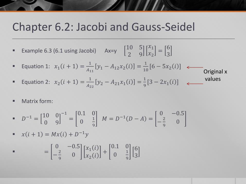
Example 6.3 (6.1 using Jacobi) Ax=y 10 52 9
𝑥1
𝑥2=
63
Equation 1: 𝑥1 𝑖 + 1 =1
𝐴11𝑦1 − 𝐴12𝑥2 𝑖 =
1
10[6 − 5𝑥2 𝑖 ]
Equation 2: 𝑥2 𝑖 + 1 =1
𝐴22𝑦2 − 𝐴21𝑥1 𝑖 =
1
9[3 − 2𝑥1 𝑖 ]
Matrix form:
𝐷−1 =10 00 9
−1
=0.1 0
01
9
𝑀 = 𝐷−1 𝐷 − 𝐴 =0 −0.5
−2
90
𝑥 𝑖 + 1 = 𝑀𝑥 𝑖 + 𝐷−1𝑦
=0 −0.5
−2
90
𝑥1 𝑖
𝑥2 𝑖+
0.1 0
01
9
63
Original x values
Chapter 6.2: Jacobi and Gauss-Seidel
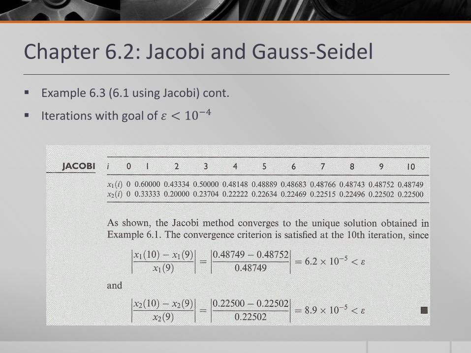
Example 6.3 (6.1 using Jacobi) cont.
Iterations with goal of 𝜀 < 10−4
Chapter 6.2: Jacobi and Gauss-Seidel
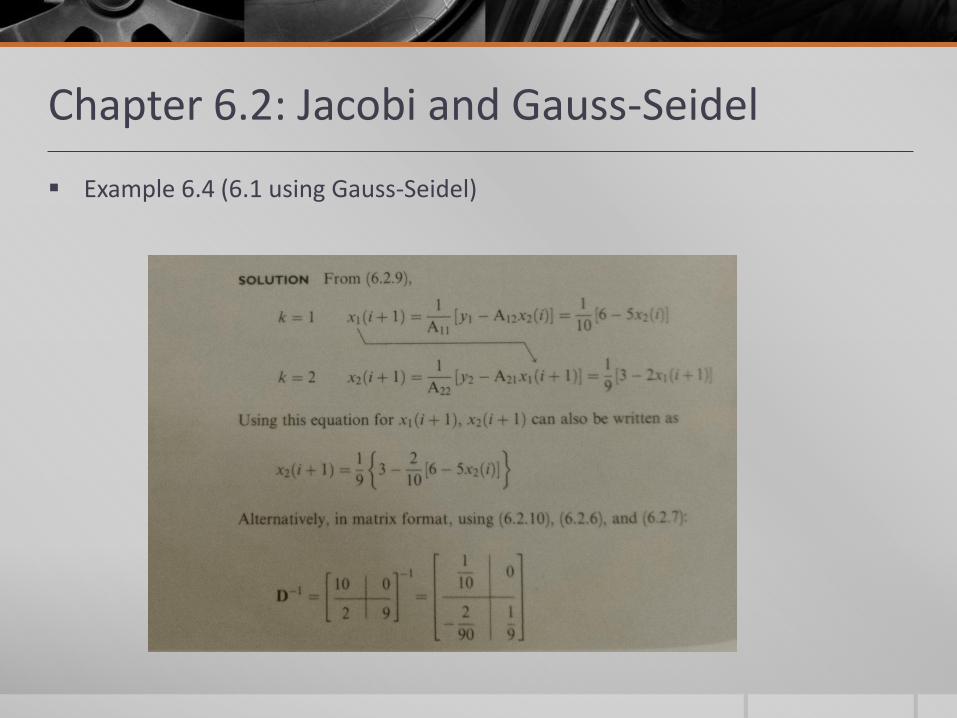
Example 6.4 (6.1 using Gauss-Seidel)
Chapter 6.2: Jacobi and Gauss-Seidel
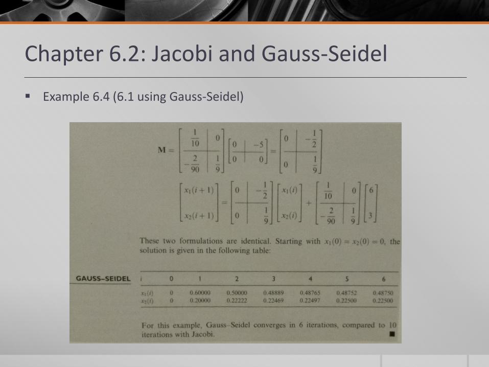
Example 6.4 (6.1 using Gauss-Seidel)
Chapter 6.2: Jacobi and Gauss-Seidel
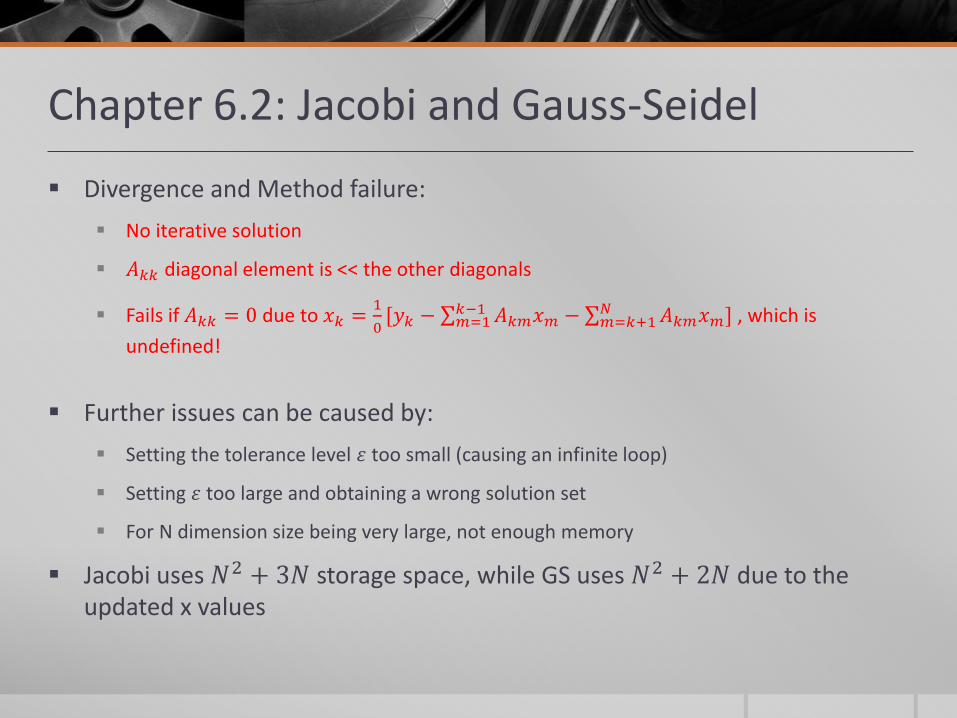
Divergence and Method failure:
No iterative solution
𝐴𝑘𝑘 diagonal element is << the other diagonals
Fails if 𝐴𝑘𝑘 = 0 due to 𝑥𝑘 =1
0[𝑦𝑘 − 𝐴𝑘𝑚𝑥𝑚
𝑘−1𝑚=1 − 𝐴𝑘𝑚𝑥𝑚
𝑁𝑚=𝑘+1 ] , which is
undefined!
Further issues can be caused by:
Setting the tolerance level 𝜀 too small (causing an infinite loop)
Setting 𝜀 too large and obtaining a wrong solution set
For N dimension size being very large, not enough memory
Jacobi uses 𝑁2 + 3𝑁 storage space, while GS uses 𝑁2 + 2𝑁 due to the updated x values
Chapter 6.2: Jacobi and Gauss-Seidel
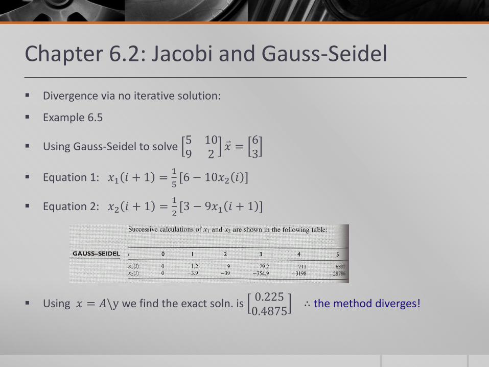
Divergence via no iterative solution:
Example 6.5
Using Gauss-Seidel to solve 5 109 2
𝑥 =63
Equation 1: 𝑥1 𝑖 + 1 =1
5[6 − 10𝑥2 𝑖 ]
Equation 2: 𝑥2 𝑖 + 1 =1
2[3 − 9𝑥1 𝑖 + 1 ]
Using 𝑥 = 𝐴\y we find the exact soln. is 0.2250.4875
∴ the method diverges!
Chapter 6.3: Newton-Raphson
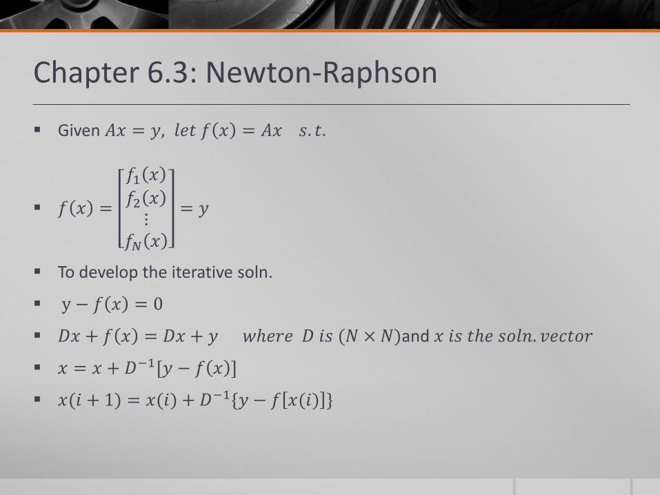
Given 𝐴𝑥 = 𝑦, 𝑙𝑒𝑡𝑓 𝑥 = 𝐴𝑥𝑠. 𝑡.
𝑓 𝑥 =
𝑓1 𝑥
𝑓2 𝑥⋮
𝑓𝑁 𝑥
= 𝑦
To develop the iterative soln.
y − 𝑓 𝑥 = 0
𝐷𝑥 + 𝑓 𝑥 = 𝐷𝑥 + 𝑦𝑤ℎ𝑒𝑟𝑒𝐷𝑖𝑠(𝑁 × 𝑁)and 𝑥𝑖𝑠𝑡ℎ𝑒𝑠𝑜𝑙𝑛. 𝑣𝑒𝑐𝑡𝑜𝑟
𝑥 = 𝑥 + 𝐷−1[𝑦 − 𝑓 𝑥 ]
𝑥(𝑖 + 1) = 𝑥(𝑖) + 𝐷−1{𝑦 − 𝑓 𝑥(𝑖) }
Chapter 6.3: Newton-Raphson
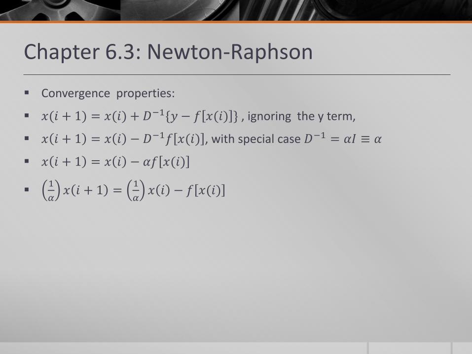
Convergence properties:
𝑥(𝑖 + 1) = 𝑥(𝑖) + 𝐷−1{𝑦 − 𝑓 𝑥(𝑖) } , ignoring the y term,
𝑥 𝑖 + 1 = 𝑥 𝑖 − 𝐷−1𝑓 𝑥(𝑖) , with special case 𝐷−1 = 𝛼𝐼 ≡ 𝛼
𝑥 𝑖 + 1 = 𝑥 𝑖 − 𝛼𝑓 𝑥(𝑖)
1
𝛼𝑥 𝑖 + 1 =
1
𝛼𝑥 𝑖 − 𝑓 𝑥(𝑖)
Chapter 6.3: Newton-Raphson
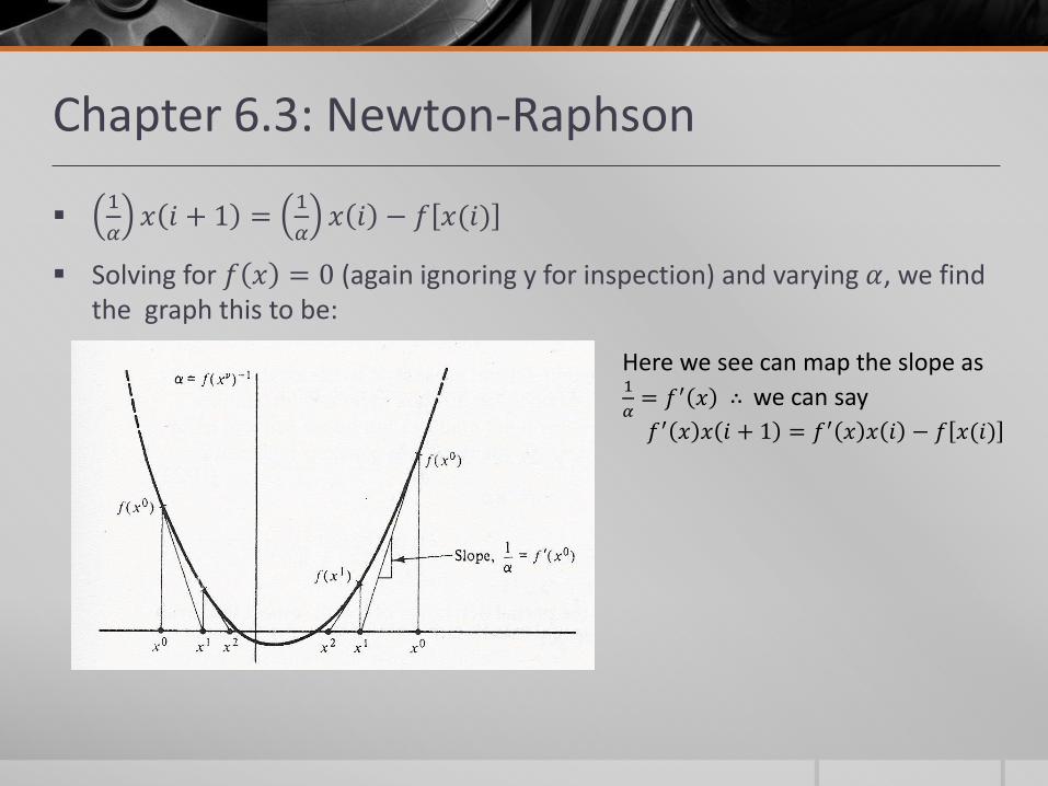
1
𝛼𝑥 𝑖 + 1 =
1
𝛼𝑥 𝑖 − 𝑓 𝑥(𝑖)
Solving for 𝑓 𝑥 = 0 (again ignoring y for inspection) and varying 𝛼, we find the graph this to be:
Here we see can map the slope as 1
𝛼= 𝑓′ 𝑥 ∴ we can say
𝑓′ 𝑥 𝑥 𝑖 + 1 = 𝑓′ 𝑥 𝑥 𝑖 − 𝑓 𝑥(𝑖)
Chapter 6.3: Newton-Raphson
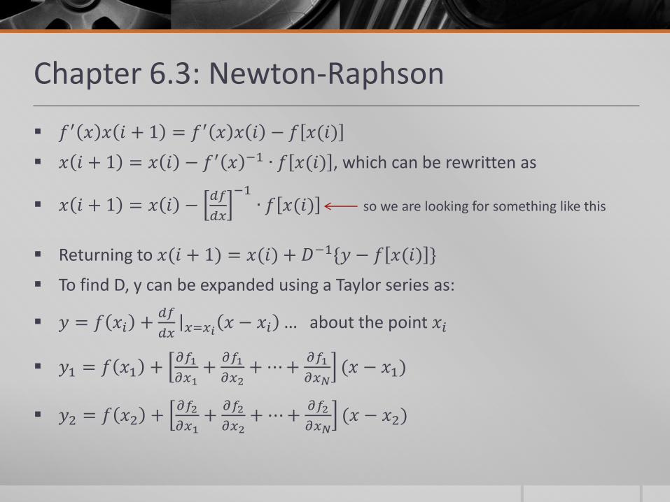
𝑓′ 𝑥 𝑥 𝑖 + 1 = 𝑓′ 𝑥 𝑥 𝑖 − 𝑓 𝑥(𝑖)
𝑥 𝑖 + 1 = 𝑥 𝑖 − 𝑓′ 𝑥 −1 ∙ 𝑓 𝑥(𝑖) , which can be rewritten as
𝑥 𝑖 + 1 = 𝑥 𝑖 −𝑑𝑓
𝑑𝑥
−1∙ 𝑓 𝑥(𝑖) so we are looking for something like this
Returning to 𝑥(𝑖 + 1) = 𝑥(𝑖) + 𝐷−1{𝑦 − 𝑓 𝑥(𝑖) }
To find D, y can be expanded using a Taylor series as:
𝑦 = 𝑓 𝑥𝑖 +𝑑𝑓
𝑑𝑥 𝑥=𝑥𝑖
𝑥 − 𝑥𝑖 … about the point 𝑥𝑖
𝑦1 = 𝑓 𝑥1 +𝜕𝑓1
𝜕𝑥1+
𝜕𝑓1
𝜕𝑥2+ ⋯+
𝜕𝑓1
𝜕𝑥𝑁(𝑥 − 𝑥1)
𝑦2 = 𝑓 𝑥2 +𝜕𝑓2
𝜕𝑥1+
𝜕𝑓2
𝜕𝑥2+ ⋯+
𝜕𝑓2
𝜕𝑥𝑁(𝑥 − 𝑥2)
Chapter 6.3: Newton-Raphson
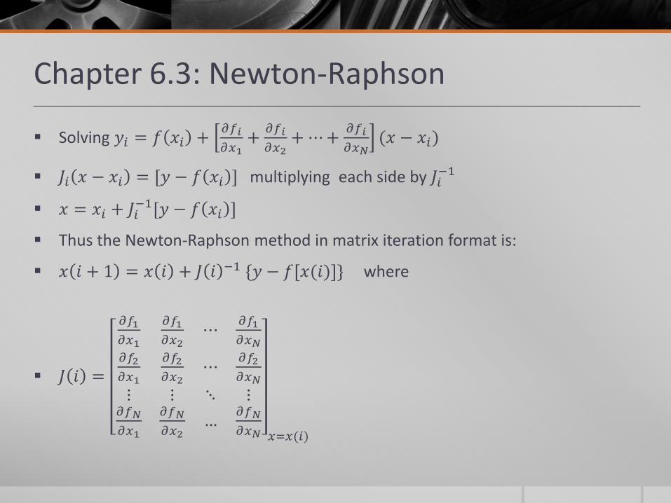
Solving 𝑦𝑖 = 𝑓 𝑥𝑖 +𝜕𝑓𝑖
𝜕𝑥1+
𝜕𝑓𝑖
𝜕𝑥2+ ⋯+
𝜕𝑓𝑖
𝜕𝑥𝑁(𝑥 − 𝑥𝑖)
𝐽𝑖 𝑥 − 𝑥𝑖 = [𝑦 − 𝑓 𝑥𝑖 ] multiplying each side by 𝐽𝑖−1
𝑥 = 𝑥𝑖 + 𝐽𝑖−1[𝑦 − 𝑓 𝑥𝑖 ]
Thus the Newton-Raphson method in matrix iteration format is:
𝑥 𝑖 + 1 = 𝑥 𝑖 + 𝐽 𝑖 −1{𝑦 − 𝑓[𝑥(𝑖)]} where
𝐽 𝑖 =
𝜕𝑓1
𝜕𝑥1
𝜕𝑓1
𝜕𝑥2⋯
𝜕𝑓1
𝜕𝑥𝑁
𝜕𝑓2
𝜕𝑥1
𝜕𝑓2
𝜕𝑥2⋯
𝜕𝑓2
𝜕𝑥𝑁
⋮ ⋮ ⋱ ⋮𝜕𝑓𝑁
𝜕𝑥1
𝜕𝑓𝑁
𝜕𝑥2…
𝜕𝑓𝑁
𝜕𝑥𝑁 𝑥=𝑥(𝑖)
Chapter 6.3: Newton-Raphson
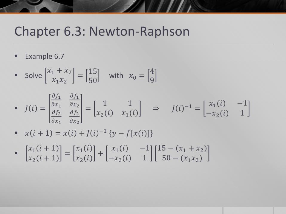
Example 6.7
Solve 𝑥1 + 𝑥2
𝑥1𝑥2=
1550
with 𝑥0 =49
𝐽 𝑖 =
𝜕𝑓1
𝜕𝑥1
𝜕𝑓1
𝜕𝑥2
𝜕𝑓2
𝜕𝑥1
𝜕𝑓2
𝜕𝑥2
=1 1
𝑥2(𝑖) 𝑥1(𝑖)⇒ 𝐽 𝑖 −1 =
𝑥1(𝑖) −1−𝑥2(𝑖) 1
𝑥 𝑖 + 1 = 𝑥 𝑖 + 𝐽 𝑖 −1{𝑦 − 𝑓[𝑥(𝑖)]}
𝑥1(𝑖 + 1)𝑥2(𝑖 + 1)
=𝑥1(𝑖)𝑥2(𝑖)
+𝑥1(𝑖) −1
−𝑥2(𝑖) 115 − (𝑥1 + 𝑥2)50 − (𝑥1𝑥2)
Chapter 6.3: Newton-Raphson
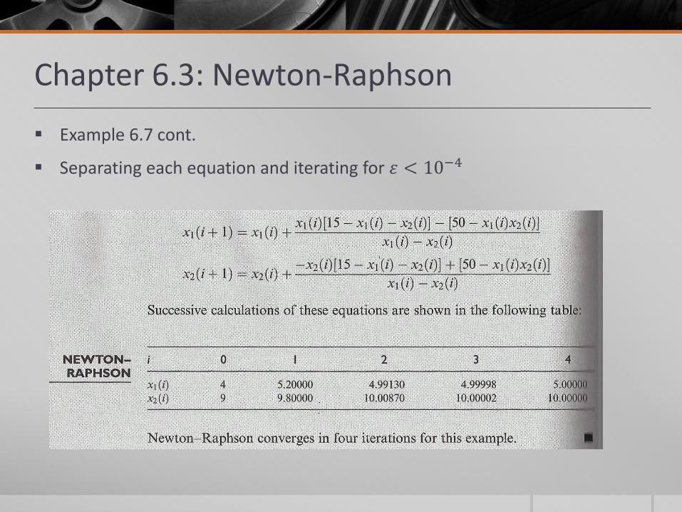
Example 6.7 cont.
Separating each equation and iterating for 𝜀 < 10−4