4.2 Modified Newton-Raphson Optimization Method

Chapter 3: Proportional hazards modelling

4.2 Modified Newton-Raphson Optimization Method

48

As mentioned earlier the modified Newton-Raphson optimization method was

found to be the most suitable to perform the likelihood maximization according to

the criteria defined above. This method is used in the case study in Chapter 4 and it

will hence be discussed in detail in this chapter.

4.2.1 Data

To simplify the discussion of the optimization technique, the form in which

the data should be arranged is defined here with specific reference to vibration

monitoring.

Suppose we have n cases of renewal, called histories, in our data and i is used to indicate the history number, i.e. i= 1,2, .. . ,n. Let I: denote time to failure or

suspension in a particular history and use cp c2 , ... , cn as event indicators such

that c; = 1 if I: is a failure time and c; = ° in case of suspension. The number

of failures present in the data is thus r = L c; .

To be able to develop the model for time-dependent covariates we set k; to be

the number of inspections or vibration measurements at moments t ij during a

certain history i over the period (0, I:] for j = 1,2, .... , k; such that:

(4.4.)

Suppose that covariate vector z~ = (Z~I' Z~2", ,,,, ,z~rn) consisting of m

covariates, is measured during history i. For convenience of estimation, it - -

could be assumed that Z;(tint) = z;(tij), where tij ~t int <t;(j+I)' The data for

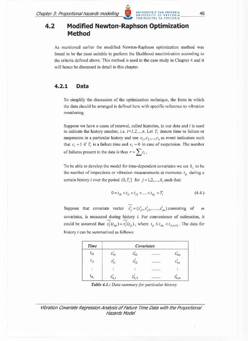
history i can be summarized as follows :

Time Co variates

tjQ ;

ZOI i

Z02 .... .... i

ZOrn

til ;

ZII ;

Z12 .. ...... i zirn

...... ..

tik; ;

Zk;1 i

Zk;2 ........ ;

zk;rn

Table 4.1.: Data summary for particular history

Vibration Covariate Regression Analysis or Failure Time Data with the Proportional Hazards Model

Chapter 3: Proportional hazards modelling 49

Some covariates can be time-independent, i.e. vary with history i, but not with

time t, or in mathematical terms z! = z~ for any valid value of s.

4.2.2 Definition of the Objective Function

The Weibull PHM as introduced in (2.17.) is repeated here for convenience as

equation (4.5.):

[ JP-1

h(t,Z(t» = ~ * · exp(y · z(t» (4.5.)

If the model in (4.5.) is transformed with an auxiliary equation a =-jJlnlJ ,

(4.5.) becomes:

h(t,z(t» = jJ. t P- 1 • exp(a + y. z(t», (4.6.)

which is more convenient for calculation procedures. We will now construct

the maximum log-likelihood function as explained in section (2.3.2) with - -

(4.6.) as a function of fl, where fl = (a,jJ'Y1 ' Y2' .... . ' Ym ) . Also assume that

c1 = c2 = .. . = cr = 1 and cr+1 = ... = cn = 0 for simplification of notation. The

log-likelihood will be of the form:

where

with

- - -/(fl) = v(fl) - u(fl),

r

v(B) = ~)n h(t;, z(tJ) ;=1

m

= ra + rlnjJ + (jJ-l) · A + LYbBb b=1

r r

A = LInt;; and Bb = Lzi;b ;=1 ;=1

Similarly for the second part of equation (4.7.):

(4.7.)

(4.8.)

(4.9.)

Vibration Covariate Regression Analysis of Failure Time Data with the Proportional Hazards Model


u(O) = :t J;i h(s,z;(s))ds i;]

(4.10.)

The most appropriate value of 8 is found where the objective function 1(8) is

a maximum, i.e. where all the partial derivatives with respect to 8 are zero or

81(0)/88) = o.

4.2.3 Partial Derivatives

- - -The first and second partial derivatives for 1(8) = v(8) - u(8) are required in

the Newton-Raphson method.

-First and second partial derivatives of v( 8) are:

- - -ov(8) = r 8v(8) = ~ + A 8v(8) = B

oa 'ojJ jJ '8Yb b (4.11.)

(4.12.)

-First and second partial derivatives of u(8) with respect to a are:

ou(8) = u(8), o2u(8) = u(8), o2u(8) = ou(8) , o2u(8) = ou(8) oa oa 2 oaojJ ojJ oaoYb OYb

(4.13.)

-First and second partial derivatives of u(8) with respect to jJ are:

-First and second partial derivatives of u( 8) with respect to Y bare:



(4.15 .)

4.2.4 Numerical Procedure

-The objective of the numerical procedure is to find the value of 8 where all

the partial derivatives are zero. Let F(B) = 81(8)/8B = (8Ij8a, 81j8jJ,81j8YI , ..

.... ,8Ij8Ym) and G(B) = 8 21/8B2

= 8 21/88i 88j . (Matrix notation IS

suppressed for convenience). The following approximation for F(8) can be - - --- -

used: F(8) ';:j F(80) + G(80)' (8 - 80 ) where 80 is an initial estimate. It is - - - -

required to solve F(80) + G(80)·(8 - 80) = 0 to determine the optimal value

of 8 .

-The conventional Newton-Raphson procedure would solve for 8 as follows:

-1. Estimate a meaningful initial value for 8, i.e. 80 •

11. Calculate F(80) and G(80).

111. Solve for ~o in the system G(80~0 = - F(80).

IV. Set 81 = 80 +~o and repeat the procedure until convergence.

Instead of the conventional Newton-Raphson method, a variable metric

method (quasi-Newton method) can be used to overcome some numerical

difficulties. In this modified Newton-Raphson method, G(8) is not calculated -

directly but an approximation of G(8) is used which is chosen to be always

positive definite, thereby eliminating the possibility of singular matrices. The

approximation of G( 8) is explained in detail in reference [80).

To accelerate convergence and increase accuracy of the procedure, the data is

transformed to more numerically convenient forms before the iteration process

is started. All recorded times, including inspection times, times to failure and

times to suspension as well as the scale parameter 1J are divided by a value C,

where:

C = (1/ N) 2> ij , (4.16.) i,j



and N is the total number of recorded times. With these scaled observations,

initial values of 170 = 3 . C and Po = 1.5 were found to be very reliable in the

numerical procedure. The covariates are also standardized to have the same

relative magnitude with the following relation:

i avg *i Z jf - Zb

zjl = (4.17.)

where

avg _ 1 ~ i d 2 _ 1 ~(i avg)2 Zb --L..JZjb an Sb --L..J Zjb - Zb '

Nb .. Nb .. I,J I,J

(4.18.)

with N b the number of recordings of a specific covariate. This standardization

of the covariates accelerates convergency considerably with initial values

Yo = 0.

Methods to vary step sizes of the procedure as well as stopping rule

procedures are discussed in Press et al. [80).

5 Goodness-of-fit Tests

Goodness-of-fit tests for the PHM are all aimed at evaluating the assumptions (see

section (2.3.)) on which the model is based. Methods to evaluate the first assumption, the

i.i.d. assumption, were discussed in section (2.1.) of Chapter 1 in considerable detail and

are not repeated here.

For the second assumption, graphical methods are usually employed to test whether an

influential covariate has been omitted from the model. Plots of estimated cumulative

hazard rates versus the number of renewals for different strata should be approximately

linear with slope equal to one, ifno influential covariate has been omitted[8I).

Two approaches can be used to test the validity of the third assumption. Graphical

techniques have been used most widely and is considered to be the first approach.[81,82,83)

The other approach is either based on hierarchical models or makes use of analytical

techniques. In the case of hierarchical models, a time-dependent covariate is introduced

into the model and tests are then performed to establish whether the estimate of the

effect of this covariate is significantly different from zero. [2,84,85,86 ) A review of these

methods is given by Kay[87).

Vibration Covariate Regression Analysis of FaIlure Time Data with the Proportional Hazards Model


5.1 Graphical Methods

Graphical methods suitable for testing the assumptions of the PHM can generally

be categorized into three groups: cumulative hazard plots, average hazards plots

and residual plots. In this discussion the emphasis is on residual plots because of its

versatility and enormous level of inherent information.

5.1.1 Cumulative Hazard Plots

Measured values of a certain covariate may often be grouped into different

levels, also referred to as strata, r. For example, the covariate Z r (t) which

occurs on s different levels and for which the proportionality assumption is to

be tested is assigned to one of the s strata. Therefore, the hazard rate in this

case can be written as:

m

hr(t, z r(t)) = hor(t)·exp( L>'j · z/t)) (5 .1.) j=l ,j#

To explain cumulative hazard plots further, consider a binary covariate Z r (t)

of which the level indicator s has two values, 0 and 1. This yields the

following in terms of total hazard rate:

m

h(t, z(t)) = ho(t)·exp( IYj ,zj(t)) · exp(Yr); (s = l) (5.2.) j=lJ#r

m

h(t,z(t)) = ho(t)·exp( IYj 'Zj(t)); (s = O) (5.3.) j=l,J-#r

Therefore, to satisfy the assumption that h(t, Z x (t)) a h(t, Z y (t)) we obtain

from (5.2.) and (5 .3.) that hOr(t) =crhO(t) for r =1,2, ... ,s where C 1'C2 ' .. . ,cs

are constants equal to exp(Yr . Zr (t)) for all strata. A similar relation holds for

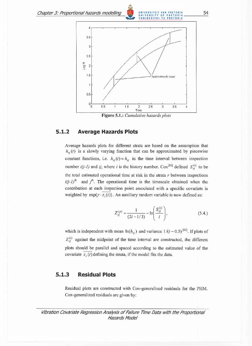
the cumulative hazard rate, i.e. H Or (t) = C rH 0 (t) . If plots of the logarithm of

the estimated cumulative hazard rates against time are constructed, they will

be shifted by an additive constant Y r , the regression parameter of a specific

stratum. Thus, if the proportionality assumption is valid, the two plots should

be approximately parallel and separated according to the different values of

the covariates. Figure 5.1. below illustrates this concept for a case where the

PHM is valid.

Vibration Covariate Regression Analysis of Failure Time Data with the Proportional Hazards ModeJ


4 ,---.----,---.----.----.---.----.---~

3.5

3

2.5

I

'" 2 .3

1.5

0.5

O ~--J---~--~----~--~--~----~--~

o 0.5 1.5 2 2.5 3 3.5 4 Time

Figure 5.1.: Cumulative hazards plots

5.1.2 Average Hazards Plots

Average hazards plots for different strata are based on the assumption that hrj (t) is a slowly varying function that can be approximated by piecewise

constant functions, i.e. hrj (t) = hrj in the time interval between inspection

number i(j-l) and ij, where i is the history number. COX[82] defined s,j) to be

the total estimated operational time at risk in the strata r between inspections

i(j-lyth and /h. The operational time is the timescale obtained when the

contribution at each inspection point associated with a specific covariate is

weighted by exp(r· Zi (t)) . An auxiliary random variable is now defined as:

Z(p) = 1 - ln~ [

S(i) )

'J (2i - 1/ 3) i ' (5.4.)

which is independent with mean In(hrj) and variance 1/(i - 0.5) [82] . Ifplots of

Z;) against the midpoint of the time interval are constructed, the different

plots should be parallel and spaced according to the estimated value of the

covariate Z r (t) defining the strata, if the model fits the data.

5.1.3 Residual Plots

Residual plots are constructed with Cox-generalized residuals for the PHM.

Cox-generalized residuals are given by:



{

U i , if ti is a failure time

ri

= U i + 1, if t i is a suspension time (5.5.)

where i = 1,2, .... , n.

In (5.5.) u i is defined as:

_ 1 ki-I - j fJ fJ Ui -7 I exp(r· Zj)· ~i(j+I) - tij ],

17 j=O

(5.6.)

with the same notation used as in section (4.2.). The calculation of u i can be

checked by noting that:

n n

LUi = r; and L ri = n , (5.7.) i=1 i=1

with r denoting the number of failures in this case. The unknowns in (5.6.) are

determined during the model fitting procedure as described in paragraph

(4.2.). With these Cox-generalized residuals known, several plots can be

constructed to assess the goodness of fit visually.

5.1.3.1 Residuals Against Order of Appearance

Here the residual for every history i = 1,2, .... ,n is plotted against the

corresponding history number, i.e. (xi;yJ = (i;1j).

The residuals should all be scattered around the straight line y = 1. Note

that the residual values of suspended cases will always be greater than 1.

If an upper limit of 1j = 3 (95%) and a lower limit of 1j = 0.05 (5%) are

chosen, it is expected that at least 90% of the residuals will fall inside

these limits if the model fits the data.

5.1.3.2 Ordered Residuals Against Expectation

If the calculated residuals 'i, 'i , .... , rn are ordered in ascending order we

get rt ~ r; ~ ..... ~ r: , the ordered residuals. The expected values of the

residuals are:

1 1 Ei =Ein =-+--+ ..... +---

, n n-l n-i+l (5.8.)

Vibration Covariate Regression Analysis of Failure Time Data WIth the Proportional Hazards Model


For a Weibull PHM that fits the data well, the points (Xi; Yi) = (Ei; rio)

will be distributed around the line Y = x. Note however that the

difference in consecutive expectations increases and that there will be a

concentration of cases below the value 1 (around 50% - 60%). The points

on the right side of the y = x line need not necessarily be close to the

line to indicate an appropriate model. This is because the variability of

the residuals increases with order number. It is possible to improve the

situation by using suitable transformations for the residuals.

To transform all points to lie between 0 and 1 with an approximately

equally spaced x-axis we could use Xi = 1 - exp( - Ei) and

Yi = 1- exp( -ri*). It is possible to stabilize the variance by using

Xi = (2/ 1r )sin -1 {exp[- (Ei /2 )]} for the x-axis and

Yi = (2/ 1r )sin -1 ~xpl- h* /2)n for the y-axis. All points will again lie

between 0 and 1. For further discussion on this method see reference [88,

89].

5.2 Analytical Goodness-of-Fit Tests

Graphical goodness-of-fit tests are often interpreted totally different by different

analysts. For this reason, analytical goodness-of-fit tests have tremendous value

since it is totally objective. Several analytical tests have been used on the PHM in

the literature, amongst others, the .%2 test, the log rank test, Z-test (normal

distribution test), Kolmogorov-Smimov test, Wald test, the doubly cumulative

hazard function, the likelihood ratio test, score tests and generalized moments

specification tests. See references [3,84,90,91,92,93,94,95,96,98] . Three of these

tests are discussed below.

5.2.1 Z-Test

Before the Z-test can be presented, some comments have to be made about

transformation rules in statistics. Transformation rules describe the changes in

the mean, variance and standard deviation of a distribution when every item in

a distribution is either increased or decreased by a constant amount. These

rules also describe the changes in the mean, variance and standard deviation of

a distribution when every item in the distribution is either multiplied or

divided by a constant amount.

• Rule 1: Adding a constant to every item in a distribution adds the constant

to the mean of the distribution, but it leaves the variance and standard



deviation unchanged.

• Rule (2): Multiplying every item in a distribution by a constant multiplies

the mean and standard deviation of that distribution by the constant and it

multiplies the variance of the distribution by the square of the constant.

The Z-test makes use of a special application of the transformation rules, the

Z-score statistic from which inferences are made. The Z-score for an event,

indicates how far and in what direction that event deviates from its

distribution's mean, expressed in units of its distribution's standard deviation.

The mathematics of the Z-score transformation are such that if every event in

a distribution is converted to its Z-score, the transformed scores will

necessarily have a mean of zero and a standard deviation of one.

For the PHM, the Z-test can be used by letting rl*:-:; r; :-:; ..... :-:; rn* be the

ordered residuals, as before, and define Zi = rio / < and m = n - 1. The Z

score for the PHM is then:

Z = ....:.i-==I,---;:==-_

~m/2 (5.9.)

Inferences about the value of Z can be made by calculating the p-value of Z,

using the normal distribution.

5.2.2 Kolmogorov-Smirnov Test

This testing procedure is classified as a frequency test of the degree of

agreement between distributions of a sample of generated random values (or a

sample of empirically gathered values) and a target distribution. Since it is

known that the residuals of the PHM should have an exponential distribution,

the Kolmogorov-Smirnov test is performed on the PHM residuals to check the

model fit.

The null hypothesis is that the cumulative density function of the PHM

residuals is equal to the cumulative density function of an exponential

distribution fitted on the residuals. To be able to test the null hypothesis, a test

statistic, called the D-statistic, is introduced. This statistic is defined as the

largest absolute difference between the Weibull PHM residuals and the

cumulative exponential distribution and inferences on the goodness-of-fit of a

model is made based on this statistic. The procedure seems simple but

becomes fairly complicated for the PHM with censored data[971.



As before, assume rl' ~ r; ~ ..... ~ r: to be the residuals ordered by magnitude

and ci to be an event indicator as defined in section (4.2.1). Let Si and a i be

sequences defined by:

( 1 )C,

s· I =S ·· 1---l+ I . n-l

(5.10.)

n (5.11.) ai+1 =ai + ( .) ( . 1) ·ci , n-l . n-l-

with So =1 , sn =exp(-rn'_I)' ao =0, an =0 and i=0,1,2, .. .. ,n-2. The D

statistic is then:

(5.12.)

From the D-statistic, a p-value can be determined to evaluate the quality of the

fit.

5.2.3 Wald Test

A test specifically developed for testing the quality of parameter estimations

by the method of maximum likelihood, is the Wald test. This test is

categorized under likelihood ratio tests and can be used to evaluate the

appropriateness of specific coefficients in the estimated regression vector and

not only the total goodness-of-fit of a model. This attribute of the Wald test is

very useful for the PHM because the contribution of different covariates to the

quality of the model can be assessed.

The Wald test statistic for a specific regression coefficient is then given by:

(5.13.)

where Yare 8 i ) is the variance of the regression coefficient and n is the sample

size. Inference on the Wald test statistic is made by calculating p-values from

the 1'2 distribution. See [98] for further details.



6 Optimal Decision Making with the Proportional Hazards Model

59

The PHM supplies us with an accurate estimate of a component's present risk to fail

(hazard rate), based on its primary use parameter and the influence of covariates. This

educated knowledge of the hazard rate should be utilized to the full to obtain economical

benefits, otherwise the PHM estimation exercise is futile.

Economical benefits from a statistical failure analysis can be guaranteed with a high

confidence level if the minimum long term life cycle cost (LeC) of a component is

determined and pursued, i.e. if renewal always takes place at either the statistical

minimum Lee or in the case of failure prior to the minimum Lee. The instant of

minimal LCC can easily be specified in terms of time for statistical models where time is

the only age parameter but for models including covariates, this makes no sense because

the covariates influence survival time.

For optimal decision making with the PHM in reliability, only one model is used in

practice, a model specifically developed for the PHM by Makis and Jardine[13,141. This

specifies the optimal renewal policy in terms of an optimal hazard rate which will lead to

the minimum Lee. At every inspection the latest hazard rate is calculated and if it

exceeds the optimal hazard rate the component is renewed, otherwise operation is

continued. If the recommendations of the decision model is obeyed, the Lee will strive

to a minimum over the long run.

To be able to determine the hazard rate that will lead to the minimum Lee it is required

to predict the behavior of covariates. Makis and Jardine's model does this by assuming

the covariate behavior to be stochastic and approximating it by a non-homogeneous

Markov chain in a finite state space. The Markov chain leads to transition probabilities

of covariates from where the optimal hazard rate is calculated.

An approach of predicting the useful remaining service life of a component and acting

preventively on the prediction rather than pursuing a statistical optimum sounds

intuitively meritorious but no research on techniques for such an approach in

conjunction with the PHM has been published up to date.

6.1 The Long Term Life Cycle Cost Concept

Lee is a concept used widely in statistical failure analysis. Several models to

achieve this minimum for repairable systems and renewal situations which depends

only on time can be found in the literature. See [15] and [22] for an overview. The



minimum Lee in renewal situations arise from two important quantities in practice

namely the cost of unexpected renewal or failure of a component, Cf , and the cost

of preventive replacement Cpo It is normally much more expensive to deal with an

unexpected failure than it is to renew preventively. A balance has to be obtained

between the risk of having to spend Cf and the advantage in the cost difference

between Cf and Cp without wasting useful remaining life of a component. The

optimum economic preventive renewal time will be at this balance point. LeC's are

usually compared when expressed as cost per unit time.

The Lee concept will be illustrated with a simple Weibull model, i.e. a model

without covariates. If a component is renewed either preventively after tp time units

or at unexpected failure for every life cycle over the long term, the total expected

cost for a life cycle would be:

(6.1.)

Since, the Lee is usually expressed m cost per unit time the average life

expectancy has to be calculated as well:

(6.2.)

where tf is the expected length of a failure cycle under the condition that failure

occurred before tp and Tp and Tf are the times required for preventive renewal and

failure renewal, respectively. When (6.1.) and (6.2.) are expressed in terms of the

Weibull reliability functions and divided into each other, the Lee per unit time, if

renewed at tp over the long term, is:

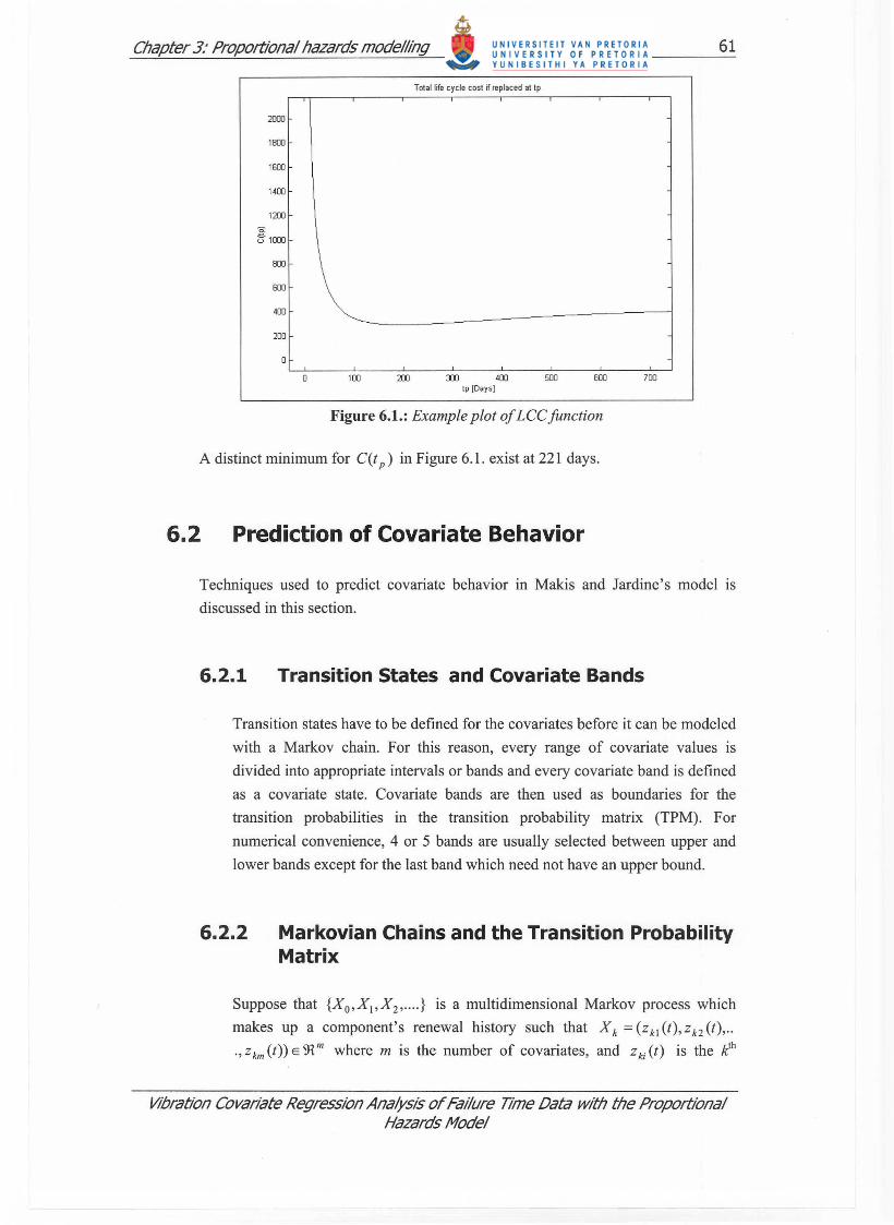
The preventive renewal time that will lead to the minimum Lee, t;, is found

where D/[C(tp)]=O. An example of (6.3.) is shown in Figure 6.1. for Weibull

parameters of jJ = 1.80 and 17 = 430 days .



TOlallife cycle cosl ~ replaced allp

2OCO

1800

1600

1400

1200

800

600

400

200

o 100 200 300 400 500 600 700 Ip [Days ]

Figure 6.1.: Example plot of LCC function

A distinct minimum for C(t p) in Figure 6.1. exist at 221 days.

6.2 Prediction of Covariate Behavior

Techniques used to predict covariate behavior in Makis and Jardine's model is

discussed in this section.

6.2.1 Transition States and Covariate Bands

Transition states have to be defined for the covariates before it can be modeled

with a Markov chain. For this reason, every range of covariate values is

divided into appropriate intervals or bands and every covariate band is defmed

as a covariate state. Covariate bands are then used as boundaries for the

transition probabilities in the transition probability matrix (TPM). For

numerical convenience, 4 or 5 bands are usually selected between upper and

lower bands except for the last band which need not have an upper bound.

6.2.2 Markovian Chains and the Transition Probability Matrix

Suppose that {Xo'X1'X2' .... } is a multidimensional Markov process which

makes up a component's renewal history such that X k = (Zkl(t),Zk2(t), ..

. , Z km (t» E 91 m where m is the number of covariates, and Z ki (t) is the klh



observation of variable i before renewal, performed at time t = kl:1,

(k = 0,1,2, .... ) while 1:1 is a fixed inspection interval. A stochastic process

{Xo'X1'X2' .. .. } is assumed to be Markovian if, for every k ~ 0,

P{Xk+1 = } IX k =i,Xk _1 =ik-l,Xk - 2 =ik - 2'·· ··· ·,X o =io}=

P{Xk+1 = } I X k = i} (6.4.)

where },i,io,ip ... , ik_1 are defined states of the process, m this case the

covariate bands.

The transition probability for any covariate in state i to undergo a transition to

state} for a given inspection interval 1:1 is :

where T denotes time to renewal as before and i and} denote any two possible

states.

Suppose we have a sample X iO , Xii' X i2 , .... and let nyCk) denote the number

of transitions from state i to} at k throughout the sample, where the sample

may contain many histories :

(6.6.)

Similarly, the number of transitions from i at time kl1 to any other state can be

calculated by:

ni(k) =# {Xk =i} = Inij(k) j

(6.7 .)

It is now possible to estimate the probability of a transition from state i to state

} at time kl1 with the following relationship derived with the maximum

likelihood method:

P,;; (k) = nij (k), k = 0,1,2, .. . " ni (k)

(6.8.)

If it is assumed that the Markov chain is homogeneous within the interval a ~ k ~ b, i.e. Pij (k) = Pij (a), the transition probability can be estimated by:



(6.9.)

It would also be possible to assume that the entire Markov chain is homogeneous, then P;j = Pij (k), for k = 0,1,2,.... and hence the transition

probabilities are estimated by:

(6.10.)

It is not realistic to assume that the transition probabilities of vibration

covariates are independent of time. For this reason continuous time is divided

into w intervals, [0,ad ,(a1,a2 ], ••••• ,(aw ,oo), in which the transition

probabilities are considered to be homogeneous. This manipulation simplifies

the calculation of the TPM tremendously without loosing much accuracy.

The estimations of the TPM above all assumed that the inspection interval ~

was constant. In practice, this is rarely the case. This would mean that

recorded data with inspection intervals different than ~ have to be omitted

from TPM calculations, thereby loosing valuable information about the

covariates' behavior. To overcome this problem a technique utilizing

transition densities (or rates) is used. Assume that the Markov chain is

homogeneous for a short interval of time. The probability of transition from i 11=0 ~ j 11 =1 is P;/t) = P(X(t) = j I X(O) = i) and the rate at which the

transition will take place is D t [Pij (t)] = Aij' (i;;/:. j) . For the case where i = j

the transition rate can be derived with the following argument. Suppose the system is in state i 11=0 and state j 11=1 with r possible states. If the sum over

all probabilities over t is taken:

P;o (t) + P;l (t) + P;2 (t) + ..... + P;r (t) = 1

Ip(X(t) = j I X(O) = i) = I j

If we take the time derivative,

or IPij(l) = I j

(6.11.)

Vibration Covariate Regression Analysis of Fal!ure Time Data with the Proportional Hazards Model


L ~[P;/t)] = 0 j at

:. ,,1,;0 + Ail + Aii + ..... + Air = 0

Aii =-LAij i#'i

The value of any Aij' (i i:- j) can be approximated by:

nij A,ii =

" Q.' I

nij = Lnij(k) k

64

(6.12.)

(6.13.)

where, k runs over the given interval of time and Qi is the total length of time

that a state is occupied in the sample. The calculation of the transition rates

can be generalized for the system from any state i to j at any time t with:

plij (t) = LP;/(t)Alj (6.14.) /

Equation (6.14.) provides a system of differential equations that has to be

solved to obtain the transition probability matrix. A solution to the system of

differential equations solution is:

p(t) = exp(A . t) , (6.15.)

where pet) = (P;/t)) and A = (Aij)' (Brackets denote matrices). This can be

calculated by the series:

(6.16.)

which is fast and accurate. Statistical tests (such as 1'2) can be used to

confirm the validity of the homogeneity assumption over the given time

intervals.

6.2.3 Calculation of the Optimal Decision Policy

Two different renewal possibilities are considered in Makis and Jardine's

model: (i) Variant 1, where preventive renewal can take place at any moment;

(ii) Variant 2, where preventive replacement can only take place at moments

of inspection. Only Variant 1 will be discussed since Variant 2 is only a

simplification of Variant 1.



A basic renewal rule is used: if the hazard rate is greater than a certain

threshold value, preventive renewal should take place otherwise operations

can continue. The objective here is thus to calculate this threshold level while

taking working age and covariates into account.

The expected average cost per unit time is a function of the threshold risk

level, d, and is given by [ '3 , '4]:

r/J(d) _ _ C-,-P _+_K_Q_(d_) - W(d) ,

(6.17.)

where K = C f - C p ' Q(d) represents the probability that failure replacement

will occur, i.e. Q(d) = P(Td ~ T) with Td the preventive renewal time at

threshold risk level d or Td = inf{t ~ 0 : h(t , Z (t)) ~ d / K} . W (d) is the

expected time until replacement, regardless of preventive action or failure, i.e.

W(d) = E(min {Td , T}) . The optimal threshold risk level, d * , is determined

with fixed point iteration to get:

r/J(d*) = min r/J(d) = d* , (6.18.) d >O

if the hazard function is non-decreasing, e.g. if jJ ~ 1 and all covariates are

non-decreasing and covariate parameters are positive. If covariates are not monotonic, then the fix point iteration does not work, and min r/J(d) should

d>O

be found by a direct search method. During the calculation of d* it is necessary to calculate Q(d) and W(d) which is no a trivial procedure. To do

this we define the covariate vector z(t) = [z'(t)'z2(t)' ...... 'zm(t)] as before

with i(t) = [i, (t), i2 (t), ..... , im (t)] the state of every covariate at time t. Thus, for

every coordinate [let Xl (il(t)) be the value of the zth covariate in state il (t)

(representative of the state) at moment t, and X(i(t)) = {X' (i, (t)) , .. .

. , Xm (irn (t))} . We could express the hazard rate now as:

[ )

/1-'

h(t, i(t)) = ~* exp(Y· X(i(t))) (6.19.)

From (2.20.), the conditional reliability function can be defined as

R(j,i,t) = P(T > jLJ + tiT> jLJ,i(t)), which becomes after substitution:

(6.20.)



with 0 ~ t ~b. . If h(t,i(t)) is a non-decreasing function in t, and if we defme

tj =inf{t~O:h(t,i(t))~d/K} and the kj's as integers such that

(k j -1~ ~ t; < kp. we can calculate the mean sojourn time of the system in

each state with:

(6.21.)

where a;=t;-(k;-I~ and r{j,i,s) = f:R(j,i,t)dt. Similarly, the

conditional cumulative distribution function for this situation is:

to, j ~k;

F(j ,i(t)) = 1- R(~,~,a;), ~ = k; -1

1- R(},l,L1),} < k; -I

(6.22.)

Let for each j, Tj = (T(j, i)); and Fj = (F(j, i)); are column vectors, and

(Pj ) = (R(j,i,L1)Pi/(j))i/ is a matrix. From here, the column vectors

Wj = (W(j, i)) and Qj = (Q(j, i)) are calculated as follows:

Wj = Tj + PjWj+1

Qj = Fj + ljQj+1 (6.23.)

Then W = W (0, io) and Q = Q(O, io), where io is an initial state of the

covariate process, usually io = ° . By starting the calculation with a large value

for j, where Wj+1 = Qj+1 = 0 and working back to 0, it is possible to solve for

Wand Q from (6.23 .). The above calculation procedure is described in detail

in [14]. A forward version of this backward calculation is numerically more

convenient and much faster (see [23]), which can be suitably adjusted for non

monotonic hazard functions also.

Thus, once the optimal threshold level is determined we renew the item at the

first moment t when:

( )

fJ-I • jJ t - - d - - exp~ .z(t))~- , 7J 7J K

(6.24.)

or, which is practically more convenient, when



d* fJ where 5* = In(_lJ_) .

K,8

Y·z(t)"2(s* - (,8 - 1)lnt,

A warning level function is defined only in terms of time by:

g(t) = 5* - (,8 -1) · In(t) ,

with g(t) strictly decreasing if ,8 > 1 .

67

(6.25.)

(6.26.)


Documents

4.2 Modified Newton-Raphson Optimization Method