Embed Size (px)
Citation preview
Algebraic Geodesy and Geoinformatics - 2009 - PART I METHODS
8 Extended Newton-Raphson Method
8- 1 Introduction
In this chapter a special numerical method is introduced, which can solve overdetermined or underdetermined systemsdirectly. Although this method is a local method, it is robust enough to handle also determined systems when the Jacobian isill- conditioned.Our problem to solve a set of nonlinear equations
f (x) = 0
where f : Âm
® Ân , namely x Î Ân
and f Î Âm.
If n = m and the Jacobi matrix has a full rank everywhere, in other words the system of equations is regular, and in addi-tion, if the initial value of the iteration is close enough to the solution, the Newton-Raphson method ensures quadraticconvergence.If one of these conditions fails, for example the system is over or under-determined, or the Jacobi matrix is singular, one canuse Extended Newton-Raphson method. Let us consider some examples to illustrate these problems.
8- 2 Overdetermined system
8- 2- 1 Overdetermined polynomial system
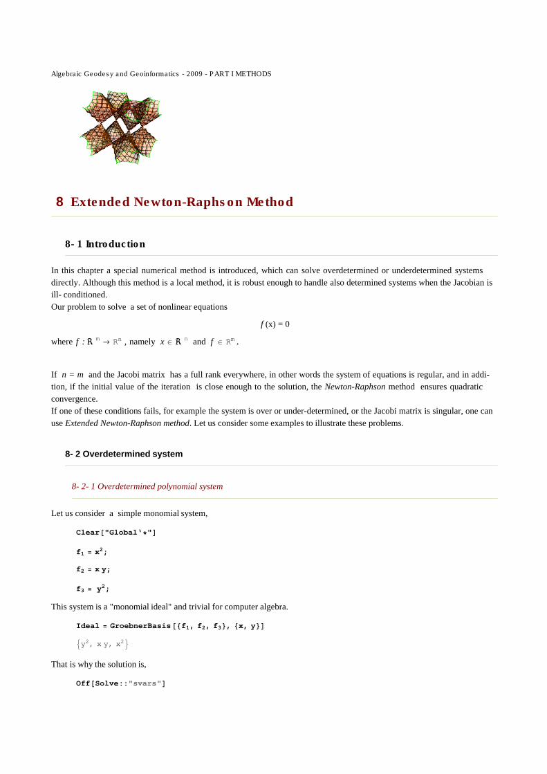
Let us consider a simple monomial system,
Clear@"Global‘*"D
f1 = x2;
f2 = x y;
f3 = y2;
This system is a "monomial ideal" and trivial for computer algebra.
Ideal = GroebnerBasis@8f1, f2, f3<, 8x, y<D
9y2, x y, x2=
That is why the solution is,
Off@Solve::"svars"D
Map@Solve@ð == 0, 8x, y<D &, IdealD
888y ® 0<, 8y ® 0<<, 88x ® 0<, 8y ® 0<<, 88x ® 0<, 8x ® 0<<<
We can see that the origin is an isolated singular root with multiplicity of 3. Global polynomial solver NSolve using
numerical Groebner basis can also solve this system,
NSolve@8f1, f2, f3<, 8x, y<D
88x ® 0., y ® 0.<, 8x ® 0., y ® 0.<, 8x ® 0., y ® 0.<<
However, standard Newton - Raphson method built in as FindRoot fails, while the system is overdetermined,
FindRoot@8f1, f2, f3<, 88x, 0.1<, 8y, 0.1<<D
FindRoot::nveq:
The number of equations does not match the number of variables in FindRoot@8f1, f2, f3<, 88x, 0.1<, 8y, 0.1<<D. �
FindRoot@8f1, f2, f3<, 88x, 0.1<, 8y, 0.1<<D
Although we can transform the overdetermined system into a determined one in sense of least squares (see ALESS). Theobjective function is the sum of the square of the residium of the equations,
obj = f12 + f2
2 + f32
x4 + x2 y2 + y4
Considering the necessary conditions for the minimum,
eqx = D@obj, xD
4 x3 + 2 x y2
eqy = D@obj, yD
2 x2 y + 4 y3
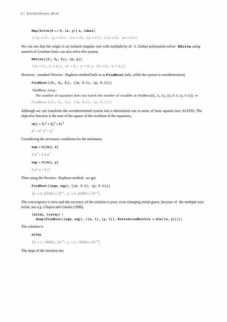
Then using the Newton - Raphson method, we get,
FindRoot@8eqx, eqy<, 88x, 0.1<, 8y, 0.1<<D
9x ® 2.03485 ´ 10-8, y ® 2.03485 ´ 10-8=
The convergence is slow and the accuracy of the solution is poor, even changing initial guess, because of the multiple rootexists, see e.g. Chapra and Canale (1998).
8solxy, listxy< =
Reap@FindRoot@8eqx, eqy<, 88x, 1<, 8y, 1<<, EvaluationMonitor ¦ Sow@8x, y<DDD;
The solution is
solxy
9x ® 1.78642 ´ 10-8, y ® 1.78642 ´ 10-8=
The steps of the iteration are,
2 ExtendedNewton_08.nb
listxy
9981., 1.<, 80.666667, 0.666667<, 80.444444, 0.444444<, 80.296296, 0.296296<,80.197531, 0.197531<, 80.131687, 0.131687<, 80.0877915, 0.0877915<,80.0585277, 0.0585277<, 80.0390184, 0.0390184<, 80.0260123, 0.0260123<,80.0173415, 0.0173415<, 80.011561, 0.011561<, 80.00770735, 0.00770735<,80.00513823, 0.00513823<, 80.00342549, 0.00342549<, 80.00228366, 0.00228366<,80.00152244, 0.00152244<, 80.00101496, 0.00101496<, 80.000676639, 0.000676639<,80.000451093, 0.000451093<, 80.000300729, 0.000300729<, 80.000200486, 0.000200486<,80.000133657, 0.000133657<, 80.0000891048, 0.0000891048<,80.0000594032, 0.0000594032<, 80.0000396021, 0.0000396021<,80.0000264014, 0.0000264014<, 80.0000176009, 0.0000176009<,80.000011734, 0.000011734<, 97.82264 ´ 10-6, 7.82264 ´ 10-6=, 95.2151 ´ 10-6, 5.2151 ´ 10-6=,93.47673 ´ 10-6, 3.47673 ´ 10-6=, 92.31782 ´ 10-6, 2.31782 ´ 10-6=,91.54521 ´ 10-6, 1.54521 ´ 10-6=, 91.03014 ´ 10-6, 1.03014 ´ 10-6=,96.86761 ´ 10-7, 6.86761 ´ 10-7=, 94.57841 ´ 10-7, 4.57841 ´ 10-7=,93.05227 ´ 10-7, 3.05227 ´ 10-7=, 92.03485 ´ 10-7, 2.03485 ´ 10-7=,91.35657 ´ 10-7, 1.35657 ´ 10-7=, 99.04377 ´ 10-8, 9.04377 ´ 10-8=,96.02918 ´ 10-8, 6.02918 ´ 10-8=, 94.01945 ´ 10-8, 4.01945 ´ 10-8=,92.67964 ´ 10-8, 2.67964 ´ 10-8=, 91.78642 ´ 10-8, 1.78642 ´ 10-8===
The error of the solution,
Norm@Last@Flatten@listxy, 1DDD
2.52639 ´ 10-8
The number of steps,
Length@Flatten@listxy, 1DD
45
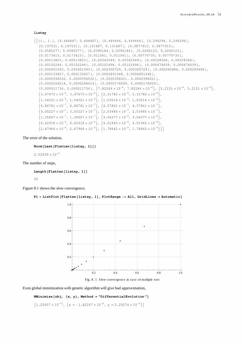
Figure 8.1 shows the slow convergence,
P1 = ListPlot@Flatten@listxy, 1D, PlotRange -> All, GridLines ® AutomaticD
0.2 0.4 0.6 0.8 1.0
0.2
0.4
0.6
0.8
1.0
Fig. 8. 1 Slow convergence in case of multiple root
Even global minimization with genetic algorithm will give bad approximation,
NMinimize@obj, 8x, y<, Method ® "DifferentialEvolution"D
91.20407 ´ 10-31, 9x ® -1.82247 ´ 10-8, y ® 5.29274 ´ 10-9==
The reason for the slow convergence is the increasing multiplicity of the root (0, 0) from 3 up to 9,
ExtendedNewton_08.nb 3
The reason for the slow convergence is the increasing multiplicity of the root (0, 0) from 3 up to 9,
NSolve@8eqx, eqy<, 8x, y<D
88x ® 0., y ® 0.<, 8x ® 0., y ® 0.<, 8x ® 0., y ® 0.<, 8x ® 0., y ® 0.<,8x ® 0., y ® 0.<, 8x ® 0., y ® 0.<, 8x ® 0., y ® 0.<, 8x ® 0., y ® 0.<, 8x ® 0., y ® 0.<<
Length@%D
9
8- 2- 2 Overdetermined non - polynomial system
A usual test problem for parameter estimation procedures is the Bard (1974) problem .
The measured data are,
data = 880.14, 1, 15, 1<,80.18, 2, 14, 2<,80.22, 3, 13, 3<,80.25, 4, 12, 4<,80.29, 5, 11, 5<,80.32, 6, 10, 6<,80.35, 7, 9, 7<,80.39, 8, 8, 8<,80.37, 9, 7, 7<,80.5, 10, 6, 6<,80.73, 11, 5, 5<,80.96, 12, 4, 4<,81.34, 13, 3, 3<,82.1, 14, 2, 2<,84.39, 15, 1, 1<<;
The system of the nonlinear equations,
eqs = MapB p1 +ð@@2DD
p2 ð@@3DD + p3 ð@@4DD- ð@@1DD &, dataF
:-0.14 + p1 +1
15 p2 + p3, -0.18 + p1 +
2
14 p2 + 2 p3, -0.22 + p1 +
3
13 p2 + 3 p3,
-0.25 + p1 +4
12 p2 + 4 p3, -0.29 + p1 +
5
11 p2 + 5 p3, -0.32 + p1 +
6
10 p2 + 6 p3,
-0.35 + p1 +7
9 p2 + 7 p3, -0.39 + p1 +
8
8 p2 + 8 p3, -0.37 + p1 +
9
7 p2 + 7 p3,
-0.5 + p1 +10
6 p2 + 6 p3, -0.73 + p1 +
11
5 p2 + 5 p3, -0.96 + p1 +
12
4 p2 + 4 p3,
-1.34 + p1 +13
3 p2 + 3 p3, -2.1 + p1 +
14
2 p2 + 2 p3, -4.39 + p1 +
15
p2 + p3>
Length@eqsD
15
We have 15 equations and 3 unknown parameters, (p1, p2, p3). The system is overdetermined and not a polynomial one. In
that case, the global polynomial solver (NSolve), Newton-Raphson method (FindRoot) as well as elimination technique
of computer algebra (GroebnerBasis) fail.
Again, one can consider the minimum of the sum of square of errors of the equations. The objective function,
4 ExtendedNewton_08.nb
Again, one can consider the minimum of the sum of square of errors of the equations. The objective function,
obj = Apply@Plus, Map@ð^2 &, eqsDD
-4.39 + p1 +15
p2 + p3
2
+ -0.14 + p1 +1
15 p2 + p3
2
+ -2.1 + p1 +14
2 p2 + 2 p3
2
+
-0.18 + p1 +2
14 p2 + 2 p3
2
+ -1.34 + p1 +13
3 p2 + 3 p3
2
+ -0.22 + p1 +3
13 p2 + 3 p3
2
+
-0.96 + p1 +12
4 p2 + 4 p3
2
+ -0.25 + p1 +4
12 p2 + 4 p3
2
+ -0.73 + p1 +11
5 p2 + 5 p3
2
+
-0.29 + p1 +5
11 p2 + 5 p3
2
+ -0.5 + p1 +10
6 p2 + 6 p3
2
+ -0.32 + p1 +6
10 p2 + 6 p3
2
+
-0.37 + p1 +9
7 p2 + 7 p3
2
+ -0.35 + p1 +7
9 p2 + 7 p3
2
+ -0.39 + p1 +8
8 p2 + 8 p3
2
Then we can find its minimum via global minimization,
AbsoluteTiming@NMinimize@obj, 8p1, p2, p3<DD
80.1562500, 80.0107093, 8p1 ® 0.0679969, p2 ® 0.889355, p3 ® 2.57247<<<
Alternatively, we can transform the problem into a determined system (ALESS). The necessary conditions of the minimum,
eq1 = D@obj, p1D
2 -4.39 + p1 +15
p2 + p3+ 2 -0.14 + p1 +
1
15 p2 + p3+ 2 -2.1 + p1 +
14
2 p2 + 2 p3+
2 -0.18 + p1 +2
14 p2 + 2 p3+ 2 -1.34 + p1 +
13
3 p2 + 3 p3+ 2 -0.22 + p1 +
3
13 p2 + 3 p3+
2 -0.96 + p1 +12
4 p2 + 4 p3+ 2 -0.25 + p1 +
4
12 p2 + 4 p3+ 2 -0.73 + p1 +
11
5 p2 + 5 p3+
2 -0.29 + p1 +5
11 p2 + 5 p3+ 2 -0.5 + p1 +
10
6 p2 + 6 p3+ 2 -0.32 + p1 +
6
10 p2 + 6 p3+
2 -0.37 + p1 +9
7 p2 + 7 p3+ 2 -0.35 + p1 +
7
9 p2 + 7 p3+ 2 -0.39 + p1 +
8
8 p2 + 8 p3
eq2 = D@obj, p2D
-
30 J-4.39 + p1 +15
p2+p3N
Hp2 + p3L2-
30 J-0.14 + p1 +1
15 p2+p3N
H15 p2 + p3L2-
56 J-2.1 + p1 +14
2 p2+2 p3N
H2 p2 + 2 p3L2-
56 J-0.18 + p1 +2
14 p2+2 p3N
H14 p2 + 2 p3L2-
78 J-1.34 + p1 +13
3 p2+3 p3N
H3 p2 + 3 p3L2-
78 J-0.22 + p1 +3
13 p2+3 p3N
H13 p2 + 3 p3L2-
96 J-0.96 + p1 +12
4 p2+4 p3N
H4 p2 + 4 p3L2-
96 J-0.25 + p1 +4
12 p2+4 p3N
H12 p2 + 4 p3L2-
110 J-0.73 + p1 +11
5 p2+5 p3N
H5 p2 + 5 p3L2-
110 J-0.29 + p1 +5
11 p2+5 p3N
H11 p2 + 5 p3L2-
120 J-0.5 + p1 +10
6 p2+6 p3N
H6 p2 + 6 p3L2-
120 J-0.32 + p1 +6
10 p2+6 p3N
H10 p2 + 6 p3L2-
126 J-0.37 + p1 +9
7 p2+7 p3N
H7 p2 + 7 p3L2-
126 J-0.35 + p1 +7
9 p2+7 p3N
H9 p2 + 7 p3L2-
128 J-0.39 + p1 +8
8 p2+8 p3N
H8 p2 + 8 p3L2
ExtendedNewton_08.nb 5
eq3 = D@obj, p3D
-
30 J-4.39 + p1 +15
p2+p3N
Hp2 + p3L2-
2 J-0.14 + p1 +1
15 p2+p3N
H15 p2 + p3L2-
56 J-2.1 + p1 +14
2 p2+2 p3N
H2 p2 + 2 p3L2-
8 J-0.18 + p1 +2
14 p2+2 p3N
H14 p2 + 2 p3L2-
78 J-1.34 + p1 +13
3 p2+3 p3N
H3 p2 + 3 p3L2-
18 J-0.22 + p1 +3
13 p2+3 p3N
H13 p2 + 3 p3L2-
96 J-0.96 + p1 +12
4 p2+4 p3N
H4 p2 + 4 p3L2-
32 J-0.25 + p1 +4
12 p2+4 p3N
H12 p2 + 4 p3L2-
110 J-0.73 + p1 +11
5 p2+5 p3N
H5 p2 + 5 p3L2-
50 J-0.29 + p1 +5
11 p2+5 p3N
H11 p2 + 5 p3L2-
120 J-0.5 + p1 +10
6 p2+6 p3N
H6 p2 + 6 p3L2-
72 J-0.32 + p1 +6
10 p2+6 p3N
H10 p2 + 6 p3L2-
126 J-0.37 + p1 +9
7 p2+7 p3N
H7 p2 + 7 p3L2-
98 J-0.35 + p1 +7
9 p2+7 p3N
H9 p2 + 7 p3L2-
128 J-0.39 + p1 +8
8 p2+8 p3N
H8 p2 + 8 p3L2
Then we can try to use Newton-Raphson method, which can be successful,
FindRoot@8eq1, eq2, eq3<, 88p1, 1<, 8p2, 1<, 8p3, 1<<D
8p1 ® 0.0679969, p2 ® 0.889355, p3 ® 2.57247<
However, this method may fail, when the starting values are far from the solution and the Jacobian becomes singular,
FindRoot@8eq1, eq2, eq3<, 88p1, -1<, 8p2, 1<, 8p3, 1<<D
FindRoot::jsing:
Encountered a singular Jacobian at the point 8p1, p2, p3< = 80.182973, 82959.2, -82955.5<. Try perturbing
the initial pointHsL. �
8p1 ® 0.182973, p2 ® 82 959.2, p3 ® -82 955.5<
Global polynomial solver with numerical Groebner basis provides solution, but besides the correct solution in sense of leastsquare, we have other real solutions. However only one positive real solution appears,
AbsoluteTiming@sol = NSolve@8eq1, eq2, eq3<, 8p1, p2, p3<DD
89.8437500, 88p1 ® 0.217315, p2 ® -8.76639, p3 ® 12.5849<,8p1 ® 0.170869 + 0.0606932 ä, p2 ® -5.99409 + 7.168 ä, p3 ® 9.59168 - 7.07904 ä<,8p1 ® 0.170869 - 0.0606932 ä, p2 ® -5.99409 - 7.168 ä, p3 ® 9.59168 + 7.07904 ä<,8p1 ® 0.22783, p2 ® -4.44817, p3 ® 8.44473<,8p1 ® 0.147587 + 0.0939871 ä, p2 ® -3.42647 + 2.4683 ä, p3 ® 6.98725 - 2.33614 ä<,8p1 ® 0.147587 - 0.0939871 ä, p2 ® -3.42647 - 2.4683 ä, p3 ® 6.98725 + 2.33614 ä<,8p1 ® 0.216599, p2 ® -2.61935, p3 ® 6.70349<,8p1 ® 0.114883 + 0.112266 ä, p2 ® -1.99681 + 1.21785 ä, p3 ® 5.51067 - 1.06593 ä<,8p1 ® 0.114883 - 0.112266 ä, p2 ® -1.99681 - 1.21785 ä, p3 ® 5.51067 + 1.06593 ä<,8p1 ® 0.181359, p2 ® -1.55169, p3 ® 5.58774<,8p1 ® 0.077954 + 0.114988 ä, p2 ® -1.15986 + 0.720556 ä, p3 ® 4.62469 - 0.570547 ä<,8p1 ® 0.077954 - 0.114988 ä, p2 ® -1.15986 - 0.720556 ä, p3 ® 4.62469 + 0.570547 ä<,8p1 ® 0.120499, p2 ® -0.852832, p3 ® 4.69769<,8p1 ® 0.0413009 + 0.102133 ä, p2 ® -0.621754 + 0.449866 ä, p3 ® 4.04119 - 0.321571 ä<,8p1 ® 0.0413009 - 0.102133 ä, p2 ® -0.621754 - 0.449866 ä, p3 ® 4.04119 + 0.321571 ä<,8p1 ® 0.0450109, p2 ® -0.386462, p3 ® 3.96801<,8p1 ® 0.0119518 + 0.0689036 ä, p2 ® -0.227926 + 0.275464 ä, p3 ® 3.61455 - 0.192522 ä<,8p1 ® 0.0119518 - 0.0689036 ä, p2 ® -0.227926 - 0.275464 ä, p3 ® 3.61455 + 0.192522 ä<,8p1 ® 0.0679969, p2 ® 0.889355, p3 ® 2.57247<<<
It goes without saying, that to compute all of these roots takes a considerable time.
The real solutions,
6 ExtendedNewton_08.nb
The real solutions,
Select@sol, And@Im@ð@@1, 2DDD � 0, Im@ð@@2, 2DDD � 0, Im@ð@@3, 2DDD � 0D &D
88p1 ® 0.217315, p2 ® -8.76639, p3 ® 12.5849<, 8p1 ® 0.22783, p2 ® -4.44817, p3 ® 8.44473<,8p1 ® 0.216599, p2 ® -2.61935, p3 ® 6.70349<, 8p1 ® 0.181359, p2 ® -1.55169, p3 ® 5.58774<,8p1 ® 0.120499, p2 ® -0.852832, p3 ® 4.69769<,8p1 ® 0.0450109, p2 ® -0.386462, p3 ® 3.96801<,8p1 ® 0.0679969, p2 ® 0.889355, p3 ® 2.57247<<
The real and positive solution,
Select@%, And@Im@ð@@1, 2DDD � 0, Im@ð@@2, 2DDD � 0,
Im@ð@@3, 2DDD � 0, Re@ð@@1, 2DDD > 0, Re@ð@@2, 2DDD > 0, Re@ð@@3, 2DDD > 0D &D88p1 ® 0.0679969, p2 ® 0.889355, p3 ® 2.57247<<
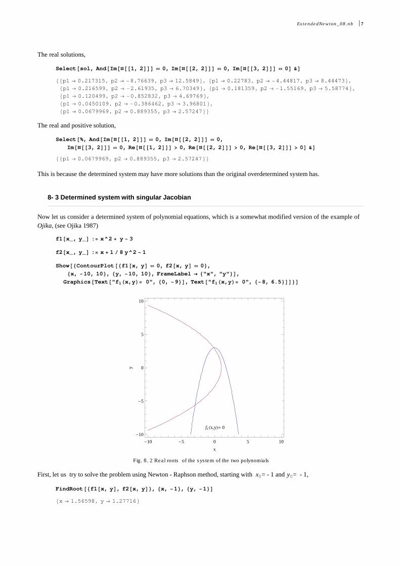
This is because the determined system may have more solutions than the original overdetermined system has.
8- 3 Determined system with singular Jacobian
Now let us consider a determined system of polynomial equations, which is a somewhat modified version of the example ofOjika, (see Ojika 1987)
f1@x_, y_D := x^2 + y - 3
f2@x_, y_D := x + 1 � 8 y^2 - 1
Show@8ContourPlot@8f1@x, yD � 0, f2@x, yD � 0<,8x, -10, 10<, 8y, -10, 10<, FrameLabel ® 8"x", "y"<D,
Graphics@Text@"f1Hx,yL= 0", 80, -9<D, Text@"f1Hx,yL= 0", 8-8, 6.5<DD<D
f1Hx,yL= 0
-10 -5 0 5 10
-10
-5
0
5
10
x
y
Fig. 8. 2 Real roots of the system of the two polynomials
First, let us try to solve the problem using Newton - Raphson method, starting with x0= - 1 and y0= - 1,
FindRoot@8f1@x, yD, f2@x, yD<, 8x, -1<, 8y, -1<D
8x ® 1.56598, y ® 1.27716<
This result is not correct,
ExtendedNewton_08.nb 7
This result is not correct,
8f1@x, yD, f2@x, yD< �. %
80.729457, 0.769873<
or starting with x0= 1 and y0= - 1,
FindRoot@8f1@x, yD, f2@x, yD<, 8x, 1<, 8y, -1<D
8x ® 1.27083, y ® 1.57379<
again, this is not a solution,
8f1@x, yD, f2@x, yD< �. %
80.188785, 0.580427<
These mean that none of them are correct solutions, Newton - Raphson method fails.
8- 4 Underdetermined system
Let us consider the following underdetermined system,
g1 = Hx - uL2 + Hy - vL2 - 1 �� Expand
-1 + u2 + v2 - 2 u x + x2 - 2 v y + y2
g2 = 2 v Hx - uL + 3 u2 Hy - vL �� Expand
-2 u v - 3 u2 v + 2 v x + 3 u2 y
g3 = I3 w u2 - 1M H2 w v - 1L �� Expand
1 - 3 u2 w - 2 v w + 6 u2 v w2
The system has infinite roots. The global polynomial solver gives some solutions,
8 ExtendedNewton_08.nb
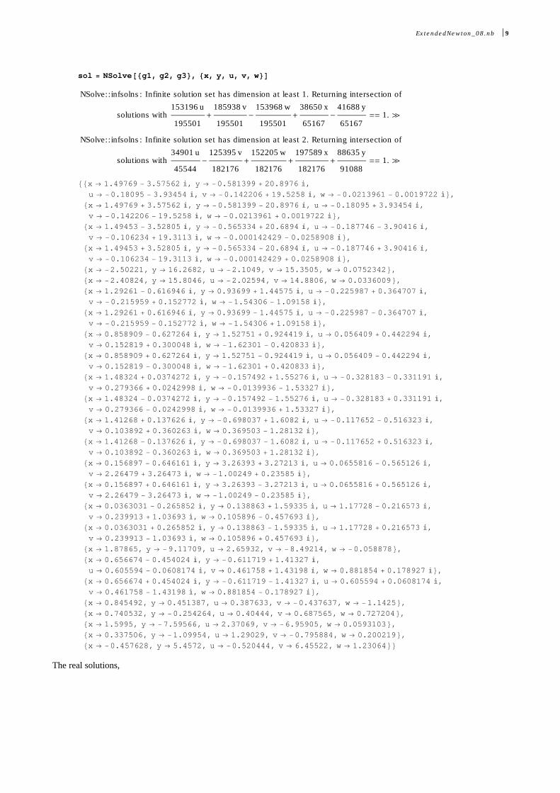
sol = NSolve@8g1, g2, g3<, 8x, y, u, v, w<D
NSolve::infsolns: Infinite solution set has dimension at least 1. Returning intersection of
solutions with153196 u
195501
+185938 v
195501
-153968 w
195501
+38650 x
65167
-41688 y
65167
== 1. �
NSolve::infsolns: Infinite solution set has dimension at least 2. Returning intersection of
solutions with34901 u
45544
-125395 v
182176
+152205 w
182176
+197589 x
182176
+88635 y
91088
== 1. �
88x ® 1.49769 - 3.57562 ä, y ® -0.581399 + 20.8976 ä,
u ® -0.18095 - 3.93454 ä, v ® -0.142206 + 19.5258 ä, w ® -0.0213961 - 0.0019722 ä<,8x ® 1.49769 + 3.57562 ä, y ® -0.581399 - 20.8976 ä, u ® -0.18095 + 3.93454 ä,
v ® -0.142206 - 19.5258 ä, w ® -0.0213961 + 0.0019722 ä<,8x ® 1.49453 - 3.52805 ä, y ® -0.565334 + 20.6894 ä, u ® -0.187746 - 3.90416 ä,
v ® -0.106234 + 19.3113 ä, w ® -0.000142429 - 0.0258908 ä<,8x ® 1.49453 + 3.52805 ä, y ® -0.565334 - 20.6894 ä, u ® -0.187746 + 3.90416 ä,
v ® -0.106234 - 19.3113 ä, w ® -0.000142429 + 0.0258908 ä<,8x ® -2.50221, y ® 16.2682, u ® -2.1049, v ® 15.3505, w ® 0.0752342<,8x ® -2.40824, y ® 15.8046, u ® -2.02594, v ® 14.8806, w ® 0.0336009<,8x ® 1.29261 - 0.616946 ä, y ® 0.93699 + 1.44575 ä, u ® -0.225987 + 0.364707 ä,
v ® -0.215959 + 0.152772 ä, w ® -1.54306 - 1.09158 ä<,8x ® 1.29261 + 0.616946 ä, y ® 0.93699 - 1.44575 ä, u ® -0.225987 - 0.364707 ä,
v ® -0.215959 - 0.152772 ä, w ® -1.54306 + 1.09158 ä<,8x ® 0.858909 - 0.627264 ä, y ® 1.52751 + 0.924419 ä, u ® 0.056409 + 0.442294 ä,
v ® 0.152819 + 0.300048 ä, w ® -1.62301 - 0.420833 ä<,8x ® 0.858909 + 0.627264 ä, y ® 1.52751 - 0.924419 ä, u ® 0.056409 - 0.442294 ä,
v ® 0.152819 - 0.300048 ä, w ® -1.62301 + 0.420833 ä<,8x ® 1.48324 + 0.0374272 ä, y ® -0.157492 + 1.55276 ä, u ® -0.328183 - 0.331191 ä,
v ® 0.279366 + 0.0242998 ä, w ® -0.0139936 - 1.53327 ä<,8x ® 1.48324 - 0.0374272 ä, y ® -0.157492 - 1.55276 ä, u ® -0.328183 + 0.331191 ä,
v ® 0.279366 - 0.0242998 ä, w ® -0.0139936 + 1.53327 ä<,8x ® 1.41268 + 0.137626 ä, y ® -0.698037 + 1.6082 ä, u ® -0.117652 - 0.516323 ä,
v ® 0.103892 + 0.360263 ä, w ® 0.369503 - 1.28132 ä<,8x ® 1.41268 - 0.137626 ä, y ® -0.698037 - 1.6082 ä, u ® -0.117652 + 0.516323 ä,
v ® 0.103892 - 0.360263 ä, w ® 0.369503 + 1.28132 ä<,8x ® 0.156897 - 0.646161 ä, y ® 3.26393 + 3.27213 ä, u ® 0.0655816 - 0.565126 ä,
v ® 2.26479 + 3.26473 ä, w ® -1.00249 + 0.23585 ä<,8x ® 0.156897 + 0.646161 ä, y ® 3.26393 - 3.27213 ä, u ® 0.0655816 + 0.565126 ä,
v ® 2.26479 - 3.26473 ä, w ® -1.00249 - 0.23585 ä<,8x ® 0.0363031 - 0.265852 ä, y ® 0.138863 + 1.59335 ä, u ® 1.17728 - 0.216573 ä,
v ® 0.239913 + 1.03693 ä, w ® 0.105896 - 0.457693 ä<,8x ® 0.0363031 + 0.265852 ä, y ® 0.138863 - 1.59335 ä, u ® 1.17728 + 0.216573 ä,
v ® 0.239913 - 1.03693 ä, w ® 0.105896 + 0.457693 ä<,8x ® 1.87865, y ® -9.11709, u ® 2.65932, v ® -8.49214, w ® -0.058878<,8x ® 0.656674 - 0.454024 ä, y ® -0.611719 + 1.41327 ä,
u ® 0.605594 - 0.0608174 ä, v ® 0.461758 + 1.43198 ä, w ® 0.881854 + 0.178927 ä<,8x ® 0.656674 + 0.454024 ä, y ® -0.611719 - 1.41327 ä, u ® 0.605594 + 0.0608174 ä,
v ® 0.461758 - 1.43198 ä, w ® 0.881854 - 0.178927 ä<,8x ® 0.845492, y ® 0.451387, u ® 0.387633, v ® -0.437637, w ® -1.1425<,8x ® 0.740532, y ® -0.254264, u ® 0.40444, v ® 0.687565, w ® 0.727204<,8x ® 1.5995, y ® -7.59566, u ® 2.37069, v ® -6.95905, w ® 0.0593103<,8x ® 0.337506, y ® -1.09954, u ® 1.29029, v ® -0.795884, w ® 0.200219<,8x ® -0.457628, y ® 5.4572, u ® -0.520444, v ® 6.45522, w ® 1.23064<<
The real solutions,
ExtendedNewton_08.nb 9
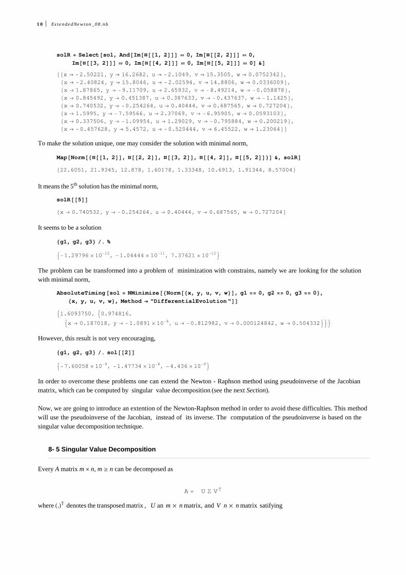
solR = Select@sol, And@Im@ð@@1, 2DDD � 0, Im@ð@@2, 2DDD � 0,
Im@ð@@3, 2DDD � 0, Im@ð@@4, 2DDD � 0, Im@ð@@5, 2DDD � 0D &D88x ® -2.50221, y ® 16.2682, u ® -2.1049, v ® 15.3505, w ® 0.0752342<,
8x ® -2.40824, y ® 15.8046, u ® -2.02594, v ® 14.8806, w ® 0.0336009<,8x ® 1.87865, y ® -9.11709, u ® 2.65932, v ® -8.49214, w ® -0.058878<,8x ® 0.845492, y ® 0.451387, u ® 0.387633, v ® -0.437637, w ® -1.1425<,8x ® 0.740532, y ® -0.254264, u ® 0.40444, v ® 0.687565, w ® 0.727204<,8x ® 1.5995, y ® -7.59566, u ® 2.37069, v ® -6.95905, w ® 0.0593103<,8x ® 0.337506, y ® -1.09954, u ® 1.29029, v ® -0.795884, w ® 0.200219<,8x ® -0.457628, y ® 5.4572, u ® -0.520444, v ® 6.45522, w ® 1.23064<<
To make the solution unique, one may consider the solution with minimal norm,
Map@Norm@8ð@@1, 2DD, ð@@2, 2DD, ð@@3, 2DD, ð@@4, 2DD, ð@@5, 2DD<D &, solRD
822.6051, 21.9345, 12.878, 1.60178, 1.33348, 10.6913, 1.91344, 8.57004<
It means the 5th
solution has the minimal norm,
solR@@5DD
8x ® 0.740532, y ® -0.254264, u ® 0.40444, v ® 0.687565, w ® 0.727204<
It seems to be a solution
8g1, g2, g3< �. %
9-1.29796 ´ 10-12, -1.04444 ´ 10-11, 7.37621 ´ 10-12=
The problem can be transformed into a problem of minimization with constrains, namely we are looking for the solutionwith minimal norm,
AbsoluteTiming@sol = NMinimize@8Norm@8x, y, u, v, w<D, g1 == 0, g2 == 0, g3 == 0<,8x, y, u, v, w<, Method ® "DifferentialEvolution"DD
91.6093750, 90.974816,9x ® 0.187018, y ® -1.0891 ´ 10-6, u ® -0.812982, v ® 0.000124842, w ® 0.504332===
However, this result is not very encouraging,
8g1, g2, g3< �. sol@@2DD
9-7.60058 ´ 10-9, -1.47734 ´ 10-8, -4.436 ´ 10-9=
In order to overcome these problems one can extend the Newton - Raphson method using pseudoinverse of the Jacobianmatrix, which can be computed by singular value decomposition (see the next Section).
Now, we are going to introduce an extention of the Newton-Raphson method in order to avoid these difficulties. This methodwill use the pseudoinverse of the Jacobian, instead of its inverse. The computation of the pseudoinverse is based on thesingular value decomposition technique.
8- 5 Singular Value Decomposition
Every A matrix m � n, m ³ n can be decomposed as
A = U S VT
where H.LTdenotes the transposed matrix , U an m ´ n matrix, and V n ´ n matrix satifying
10 ExtendedNewton_08.nb
UT U = VT V = V VT = In
and S = < Σ1, ..., Σn > a diagonal matrix.
These Σi ’ s, Σ1 ³ Σ2 ³, ..., Σn ³ 0 are the square root of the non negative eigenvalues of AT
A
and are called as the singular values of matrix A.
As it is known from linear algebra, singular value decomposition (SVD) is a technique to compute pseudoinverse forsingular or ill-conditioned matrix of linear systems. In addition this method provides least square solution for overdeter-
mined system and minimal norm solution in case of undetermined system.
8- 6 Pseudoinverse
The pseudoinverse of a matrix A of m ´ n is a matrix A+
of n ´ m satisfying
A A+ A = A , A+ A A+ = A+, HA+ AL*= A+ A, HA A+L*
= A A+
where H.L*denotes the conjugate transpose of the matrix.
There always exists a unique A+
whic can be computed using SVD :
aL If m ³ n and A = U S VT
then
A+ = V S-1 UT
where S-1 = < 1 � Σ1, ..., 1 � Σn >
b) If m < n then compute the HATL+, pseudoinverse of AT and then
A+ = IIATM+MT
8- 7 Newton - Raphson Method with Pseudoinverse
The idea of using pseudoinverse in order to generalize of Newton-Raphson method is not new, see e.g. Quoc - Nam Tran
(1998). It means that in the iteration formula, the pseudoinverse of the Jacobian matrix will be employed,
xi+1 = xi - J+ HxiL f HxiL
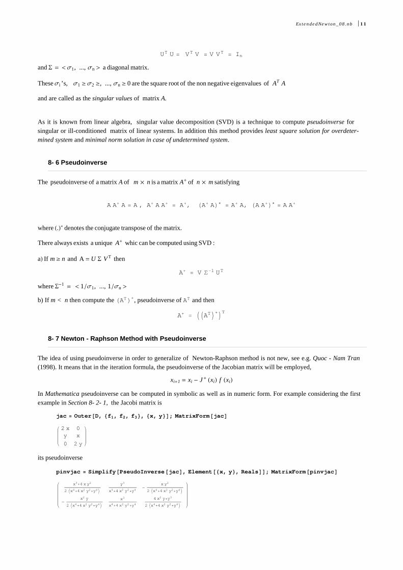
In Mathematica pseudoinverse can be computed in symbolic as well as in numeric form. For example considering the firstexample in Section 8- 2- 1, the Jacobi matrix is
jac = Outer@D, 8f1, f2, f3<, 8x, y<D; MatrixForm@jacD
2 x 0y x
0 2 y
its pseudoinverse
pinvjac = Simplify@PseudoInverse@jacD, Element@8x, y<, RealsDD; MatrixForm@pinvjacDx3+4 x y2
2 Ix4+4 x2 y2+y4My3
x4+4 x2 y2+y4-
x y2
2 Ix4+4 x2 y2+y4M
-x2 y
2 Ix4+4 x2 y2+y4Mx3
x4+4 x2 y2+y4
4 x2 y+y3
2 Ix4+4 x2 y2+y4M
In numerical form the Jacobi matrix at the point (x, y) = (1, 1)
ExtendedNewton_08.nb 11
In numerical form the Jacobi matrix at the point (x, y) = (1, 1)
jacN = jac �. 8x -> 1., y -> 1.<; MatrixForm@jacND
2. 0
1. 1.
0 2.
and its pseudoinverse,
pinvjacN = PseudoInverse@jacND; MatrixForm@pinvjacND
K 0.416667 0.166667 -0.0833333
-0.0833333 0.166667 0.416667O
or
Hpinvjac �. 8x -> 1., y -> 1.<L �� MatrixForm
K 0.416667 0.166667 -0.0833333
-0.0833333 0.166667 0.416667O
The new values (xi+1, yi+1) in the next iteration step are
81, 1< - pinvjacN.H8f1, f2, f3< �. 8x -> 1., y -> 1.<L
80.5, 0.5<
8- 8 Implementation in Mathematica
The implementation is a modified adoptation of the function written by Ruskeepä ä , (see Ruskeepä ä 2009)
NewtonExtended@f_List, x_List, x0_List, eps_: 10^-12, n_: 100D :=
With@8jac = N@Outer@D, f, xDD<,FixedPointList@Hð + PseudoInverse@jac �. Thread@x ® N@ðDDD.H-f �. Thread@x ® N@ðDDLL &,
N@x0D, n, SameTest ® HSqrt@Abs@Hð1 - ð2L.Hð1 - ð2LDD < eps &LDD
where
f - the list of the equations of the system, 8 f1, ..., fm<
x - the list of the variables of the system, x = 8x1, ... xn<
x0 - the list of the numerical start value of the iteration, x0 = 8x01, ... x0n<
eps - the limit of the error , employing Frobenius norm, the default value is 10^-12
n - the maximum number of the iterations, the default value is 100
In the following section we shall solve the four different problems introduced above with this method.
12 ExtendedNewton_08.nb
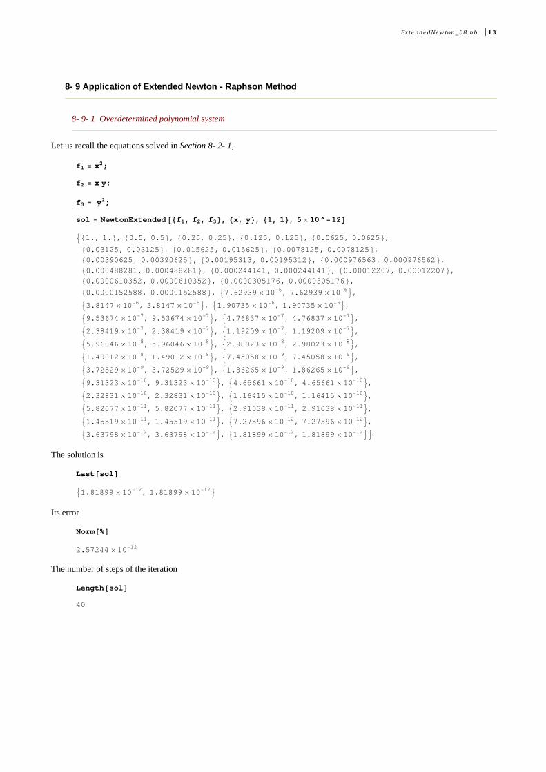
8- 9 Application of Extended Newton - Raphson Method
8- 9- 1 Overdetermined polynomial system
Let us recall the equations solved in Section 8- 2- 1,
f1 = x2;
f2 = x y;
f3 = y2;
sol = NewtonExtended@8f1, f2, f3<, 8x, y<, 81, 1<, 5 ´ 10^-12D
981., 1.<, 80.5, 0.5<, 80.25, 0.25<, 80.125, 0.125<, 80.0625, 0.0625<,80.03125, 0.03125<, 80.015625, 0.015625<, 80.0078125, 0.0078125<,80.00390625, 0.00390625<, 80.00195313, 0.00195312<, 80.000976563, 0.000976562<,80.000488281, 0.000488281<, 80.000244141, 0.000244141<, 80.00012207, 0.00012207<,80.0000610352, 0.0000610352<, 80.0000305176, 0.0000305176<,80.0000152588, 0.0000152588<, 97.62939 ´ 10-6, 7.62939 ´ 10-6=,93.8147 ´ 10-6, 3.8147 ´ 10-6=, 91.90735 ´ 10-6, 1.90735 ´ 10-6=,99.53674 ´ 10-7, 9.53674 ´ 10-7=, 94.76837 ´ 10-7, 4.76837 ´ 10-7=,92.38419 ´ 10-7, 2.38419 ´ 10-7=, 91.19209 ´ 10-7, 1.19209 ´ 10-7=,95.96046 ´ 10-8, 5.96046 ´ 10-8=, 92.98023 ´ 10-8, 2.98023 ´ 10-8=,91.49012 ´ 10-8, 1.49012 ´ 10-8=, 97.45058 ´ 10-9, 7.45058 ´ 10-9=,93.72529 ´ 10-9, 3.72529 ´ 10-9=, 91.86265 ´ 10-9, 1.86265 ´ 10-9=,99.31323 ´ 10-10, 9.31323 ´ 10-10=, 94.65661 ´ 10-10, 4.65661 ´ 10-10=,92.32831 ´ 10-10, 2.32831 ´ 10-10=, 91.16415 ´ 10-10, 1.16415 ´ 10-10=,95.82077 ´ 10-11, 5.82077 ´ 10-11=, 92.91038 ´ 10-11, 2.91038 ´ 10-11=,91.45519 ´ 10-11, 1.45519 ´ 10-11=, 97.27596 ´ 10-12, 7.27596 ´ 10-12=,93.63798 ´ 10-12, 3.63798 ´ 10-12=, 91.81899 ´ 10-12, 1.81899 ´ 10-12==
The solution is
Last@solD
91.81899 ´ 10-12, 1.81899 ´ 10-12=
Its error
Norm@%D
2.57244 ´ 10-12
The number of steps of the iteration
Length@solD
40
ExtendedNewton_08.nb 13
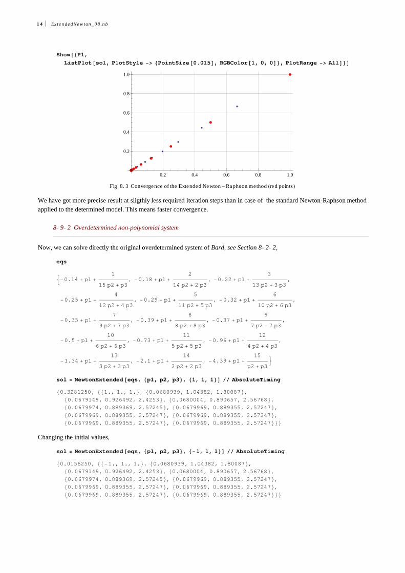
Show@8P1,ListPlot@sol, PlotStyle -> [email protected], RGBColor@1, 0, 0D<, PlotRange -> AllD<D
0.2 0.4 0.6 0.8 1.0
0.2
0.4
0.6
0.8
1.0
Fig. 8. 3 Convergence of the Extended Newton - Raphson method Hred pointsL
We have got more precise result at sligthly less required iteration steps than in case of the standard Newton-Raphson methodapplied to the determined model. This means faster convergence.
8- 9- 2 Overdetermined non-polynomial system
Now, we can solve directly the original overdetermined system of Bard, see Section 8- 2- 2,
eqs
:-0.14 + p1 +1
15 p2 + p3, -0.18 + p1 +
2
14 p2 + 2 p3, -0.22 + p1 +
3
13 p2 + 3 p3,
-0.25 + p1 +4
12 p2 + 4 p3, -0.29 + p1 +
5
11 p2 + 5 p3, -0.32 + p1 +
6
10 p2 + 6 p3,
-0.35 + p1 +7
9 p2 + 7 p3, -0.39 + p1 +
8
8 p2 + 8 p3, -0.37 + p1 +
9
7 p2 + 7 p3,
-0.5 + p1 +10
6 p2 + 6 p3, -0.73 + p1 +
11
5 p2 + 5 p3, -0.96 + p1 +
12
4 p2 + 4 p3,
-1.34 + p1 +13
3 p2 + 3 p3, -2.1 + p1 +
14
2 p2 + 2 p3, -4.39 + p1 +
15
p2 + p3>
sol = NewtonExtended@eqs, 8p1, p2, p3<, 81, 1, 1<D �� AbsoluteTiming
80.3281250, 881., 1., 1.<, 80.0680939, 1.04382, 1.80087<,80.0679149, 0.926492, 2.4253<, 80.0680004, 0.890657, 2.56768<,80.0679974, 0.889369, 2.57245<, 80.0679969, 0.889355, 2.57247<,80.0679969, 0.889355, 2.57247<, 80.0679969, 0.889355, 2.57247<,80.0679969, 0.889355, 2.57247<, 80.0679969, 0.889355, 2.57247<<<
Changing the initial values,
sol = NewtonExtended@eqs, 8p1, p2, p3<, 8-1, 1, 1<D �� AbsoluteTiming
80.0156250, 88-1., 1., 1.<, 80.0680939, 1.04382, 1.80087<,80.0679149, 0.926492, 2.4253<, 80.0680004, 0.890657, 2.56768<,80.0679974, 0.889369, 2.57245<, 80.0679969, 0.889355, 2.57247<,80.0679969, 0.889355, 2.57247<, 80.0679969, 0.889355, 2.57247<,80.0679969, 0.889355, 2.57247<, 80.0679969, 0.889355, 2.57247<<<
Again, Extended Newton - Raphson Method is robust, as well as faster than NSolve, becasue we do not need to compute
all roots, especially not the all roots of the squared system (ALESS)!
14 ExtendedNewton_08.nb
Again, Extended Newton - Raphson Method is robust, as well as faster than NSolve, becasue we do not need to compute
all roots, especially not the all roots of the squared system (ALESS)!
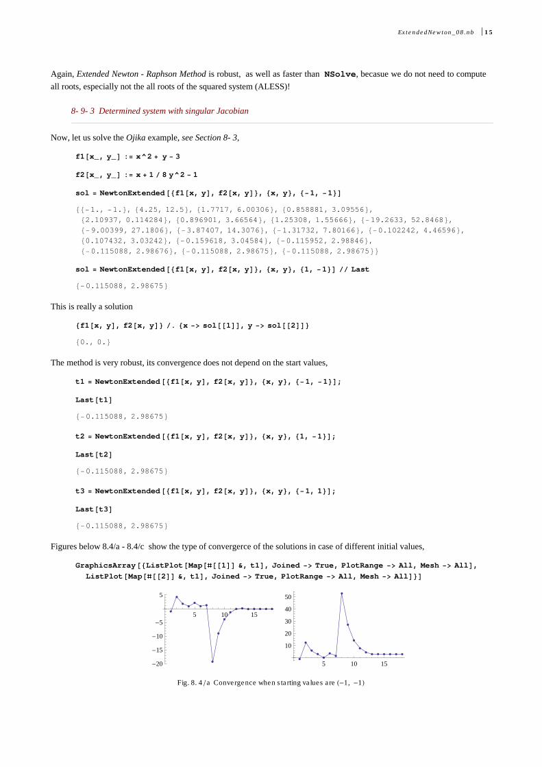
8- 9- 3 Determined system with singular Jacobian
Now, let us solve the Ojika example, see Section 8- 3,
f1@x_, y_D := x^2 + y - 3
f2@x_, y_D := x + 1 � 8 y^2 - 1
sol = NewtonExtended@8f1@x, yD, f2@x, yD<, 8x, y<, 8-1, -1<D
88-1., -1.<, 84.25, 12.5<, 81.7717, 6.00306<, 80.858881, 3.09556<,82.10937, 0.114284<, 80.896901, 3.66564<, 81.25308, 1.55666<, 8-19.2633, 52.8468<,8-9.00399, 27.1806<, 8-3.87407, 14.3076<, 8-1.31732, 7.80166<, 8-0.102242, 4.46596<,80.107432, 3.03242<, 8-0.159618, 3.04584<, 8-0.115952, 2.98846<,8-0.115088, 2.98676<, 8-0.115088, 2.98675<, 8-0.115088, 2.98675<<
sol = NewtonExtended@8f1@x, yD, f2@x, yD<, 8x, y<, 81, -1<D �� Last
8-0.115088, 2.98675<
This is really a solution
8f1@x, yD, f2@x, yD< �. 8x -> sol@@1DD, y -> sol@@2DD<
80., 0.<
The method is very robust, its convergence does not depend on the start values,
t1 = NewtonExtended@8f1@x, yD, f2@x, yD<, 8x, y<, 8-1, -1<D;
Last@t1D
8-0.115088, 2.98675<
t2 = NewtonExtended@8f1@x, yD, f2@x, yD<, 8x, y<, 81, -1<D;
Last@t2D
8-0.115088, 2.98675<
t3 = NewtonExtended@8f1@x, yD, f2@x, yD<, 8x, y<, 8-1, 1<D;
Last@t3D
8-0.115088, 2.98675<
Figures below 8.4/a - 8.4/c show the type of convergerce of the solutions in case of different initial values,
GraphicsArray@8ListPlot@Map@ð@@1DD &, t1D, Joined -> True, PlotRange -> All, Mesh -> AllD,ListPlot@Map@ð@@2DD &, t1D, Joined -> True, PlotRange -> All, Mesh -> AllD<D
5 10 15
-20
-15
-10
-5
5
5 10 15
10
20
30
40
50
Fig. 8. 4 � a Convergence when starting values are H-1, -1L
ExtendedNewton_08.nb 15
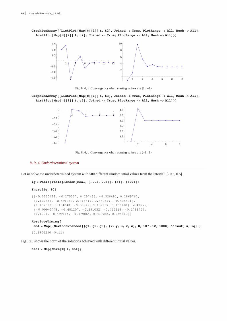
GraphicsArray@8ListPlot@Map@ð@@1DD &, t2D, Joined -> True, PlotRange -> All, Mesh -> AllD,ListPlot@Map@ð@@2DD &, t2D, Joined -> True, PlotRange -> All, Mesh -> AllD<D
2 4 6 8 10 12
-1.5
-1.0
-0.5
0.5
1.0
1.5
2 4 6 8 10 12
2
4
6
8
10
Fig. 8. 4 � b Convergency when starting values are H1, -1L
GraphicsArray@8ListPlot@Map@ð@@1DD &, t3D, Joined -> True, PlotRange -> All, Mesh -> AllD,ListPlot@Map@ð@@2DD &, t3D, Joined -> True, PlotRange -> All, Mesh -> AllD<D
2 4 6 8
-1.0
-0.8
-0.6
-0.4
-0.2
2 4 6 8
1.5
2.0
2.5
3.0
3.5
4.0
Fig. 8. 4 � c Convergency when starting values are H-1, 1L
8- 9- 4 Underdetermined system
Let us solve the underdetermined system with 500 different random intial values from the intervall [- 0.5, 0.5].
ig = Table@Table@Random@Real, 8-0.5, 0.5<D, 85<D, 8500<D;
Short@ig, 10D
88-0.0550423, -0.275307, 0.157435, -0.328481, 0.186976<,80.199535, -0.491282, 0.364317, 0.330879, -0.435401<,80.407528, 0.134848, -0.38972, 0.132237, 0.103198<, �495�,
8-0.00945778, -0.481257, -0.291032, -0.435218, -0.178875<,80.1991, -0.499865, -0.479864, 0.417085, 0.194819<<
AbsoluteTiming@sol = Map@HNewtonExtended@8g1, g2, g3<, 8x, y, u, v, w<, ð, 10^-12, 1000D �� LastL &, igD;D
80.8906250, Null<
Fig . 8.5 shows the norm of the solutions achieved with different initial values,
nsol = Map@Norm@ðD &, solD;
16 ExtendedNewton_08.nb
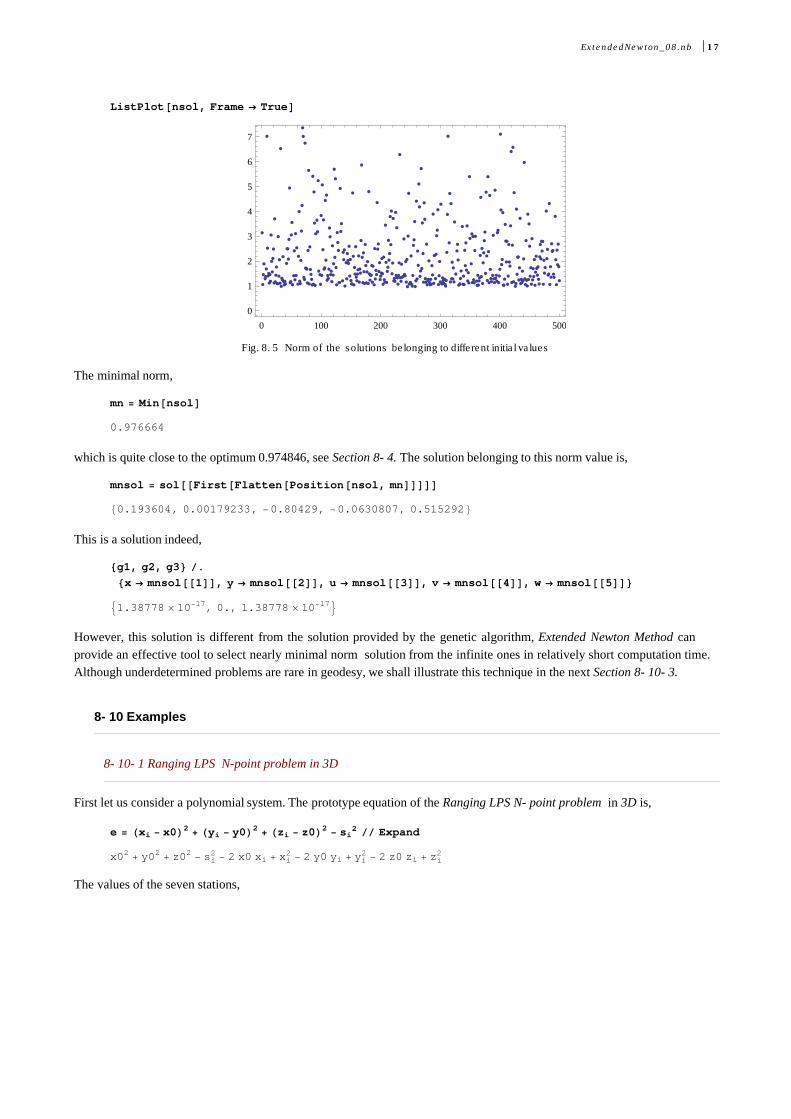
ListPlot@nsol, Frame ® TrueD
0 100 200 300 400 500
0
1
2
3
4
5
6
7
Fig. 8. 5 Norm of the solutions belonging to different initial values
The minimal norm,
mn = Min@nsolD
0.976664
which is quite close to the optimum 0.974846, see Section 8- 4. The solution belonging to this norm value is,
mnsol = sol@@First@Flatten@Position@nsol, mnDDDDD
80.193604, 0.00179233, -0.80429, -0.0630807, 0.515292<
This is a solution indeed,
8g1, g2, g3< �.8x ® mnsol@@1DD, y ® mnsol@@2DD, u ® mnsol@@3DD, v ® mnsol@@4DD, w ® mnsol@@5DD<
91.38778 ´ 10-17, 0., 1.38778 ´ 10-17=
However, this solution is different from the solution provided by the genetic algorithm, Extended Newton Method canprovide an effective tool to select nearly minimal norm solution from the infinite ones in relatively short computation time.Although underdetermined problems are rare in geodesy, we shall illustrate this technique in the next Section 8- 10- 3.
8- 10 Examples
8- 10- 1 Ranging LPS N-point problem in 3D
First let us consider a polynomial system. The prototype equation of the Ranging LPS N- point problem in 3D is,
e = Hxi - x0L2 + Hyi - y0L2 + Hzi - z0L2 - si2 �� Expand
x02 + y02 + z02 - si2 - 2 x0 xi + xi
2 - 2 y0 yi + yi2 - 2 z0 zi + zi
2
The values of the seven stations,
ExtendedNewton_08.nb 17
datan = 8x1 -> 4 157 246.5346, y1 -> 671 877.0281, z1 -> 4 774 581.6314, s1 -> 566.8635,
x2 -> 4 156 749.5977, y2 -> 672 711.4554, z2 -> 4 774 981.5459, s2 -> 1324.2380,
x3 -> 4 156 748.6829, y3 -> 671 171.9385, z3 -> 4 775 235.5483, s3 -> 542.2609,
x4 -> 4 157 066.8851, y4 -> 671 064.9381, z4 -> 4 774 865.8238, s4 -> 364.9797,
x5 -> 4 157 266.6181, y5 -> 671 099.1577, z5 -> 4 774 689.8536, s5 -> 430.5286,
x6 -> 4 157 307.5147, y6 -> 671 171.7006, z6 -> 4 774 690.5691, s6 -> 400.5837,
x7 -> 4 157 244.9515, y7 -> 671 338.5915, z7 -> 4 774 699.9070, s7 -> 269.2309
<;
The system to be solved in numerical form,
F = Table@e �. datan, 8i, 1, 7<D �� Expand
94.05307 ´ 1013 - 8.31449 ´ 106 x0 + x02 - 1.34375 ´ 106 y0 + y02 - 9.54916 ´ 106 z0 + z02,
4.05316 ´ 1013 - 8.3135 ´ 106 x0 + x02 - 1.34542 ´ 106 y0 + y02 - 9.54996 ´ 106 z0 + z02,
4.05319 ´ 1013 - 8.3135 ´ 106 x0 + x02 - 1.34234 ´ 106 y0 + y02 - 9.55047 ´ 106 z0 + z02,
4.05309 ´ 1013 - 8.31413 ´ 106 x0 + x02 - 1.34213 ´ 106 y0 + y02 - 9.54973 ´ 106 z0 + z02,
4.05309 ´ 1013 - 8.31453 ´ 106 x0 + x02 - 1.3422 ´ 106 y0 + y02 - 9.54938 ´ 106 z0 + z02,
4.05313 ´ 1013 - 8.31462 ´ 106 x0 + x02 - 1.34234 ´ 106 y0 + y02 - 9.54938 ´ 106 z0 + z02,
4.05311 ´ 1013 - 8.31449 ´ 106 x0 + x02 - 1.34268 ´ 106 y0 + y02 - 9.5494 ´ 106 z0 + z02=
The variables,
X = 8x0, y0, z0<
8x0, y0, z0<
In order to find initial value, we consider the linear part of the system equations,
eL = -si2 - 2 x0 xi + xi
2 - 2 y0 yi + yi2 - 2 z0 zi + zi
2;
This linear system in numerical form,
G = Table@eL �. datan, 8i, 1, 7<D �� Expand
94.05307 ´ 1013 - 8.31449 ´ 106 x0 - 1.34375 ´ 106 y0 - 9.54916 ´ 106 z0,
4.05316 ´ 1013 - 8.3135 ´ 106 x0 - 1.34542 ´ 106 y0 - 9.54996 ´ 106 z0,
4.05319 ´ 1013 - 8.3135 ´ 106 x0 - 1.34234 ´ 106 y0 - 9.55047 ´ 106 z0,
4.05309 ´ 1013 - 8.31413 ´ 106 x0 - 1.34213 ´ 106 y0 - 9.54973 ´ 106 z0,
4.05309 ´ 1013 - 8.31453 ´ 106 x0 - 1.3422 ´ 106 y0 - 9.54938 ´ 106 z0,
4.05313 ´ 1013 - 8.31462 ´ 106 x0 - 1.34234 ´ 106 y0 - 9.54938 ´ 106 z0,
4.05311 ´ 1013 - 8.31449 ´ 106 x0 - 1.34268 ´ 106 y0 - 9.5494 ´ 106 z0=
The guess value for the Extended Newton- Raphson method will be the least square solution of this linear system,
8b, A< = CoefficientArrays@G, 8x0, y0, z0<D; b = -b;
x0y0z0 = LeastSquares@Normal@AD, Normal@bDD
91.88181 ´ 106, 323 070., 2.56048 ´ 106=
Therefore
X0 = x0y0z0
91.88181 ´ 106, 323 070., 2.56048 ´ 106=
Then
AbsoluteTiming@NewtonExtended@F, X, X0D �� LastD
90.0781250, 94.15707 ´ 106, 671 430., 4.77488 ´ 106==
18 ExtendedNewton_08.nb
NumberForm@%, 12D
90.0781250, 94.15706611149 ´ 106, 671429.665473, 4.77487937028 ´ 106==
This example clearly demonstrates the robustness of the method!
8- 10- 2 GPS N-point problem
Let us solve the GPS - N point problem employing the solutions of the different subsets of the Gauss- Jacobi combinatorialtechnique computed in the previous chapter. Now, we employ the distance error model, namely the general form of theequations is,
en = di - Hx1 - aiL2 + Hx2 - biL2 + Hx3 - ciL2 - x4 ;
The values of the 6 satellites are,
datan = 8a0 ® 14 177 553.47, a1 ® 15 097 199.81,
a2 ® 23 460 342.33, a3 ® -8 206 488.95, a4 ® 1 399 988.07, a5 ® 6 995 655.48,
b0 ® -18 814 768.09, b1 ® -4 636 088.67, b2 ® -9 433 518.58,
b3 ® -18 217 989.14, b4 ® -17 563 734.90, b5 ® -23 537 808.26,
c0 ® 12 243 866.38, c1 ® 21 326 706.55, c2 ® 8 174 941.25,
c3 ® 17 605 231.99, c4 ® 19 705 591.18, c5 ® -9 927 906.48,
d0 ® 21 119 278.32, d1 ® 22 527 064.18, d2 ® 23 674 159.88,
d3 ® 20 951 647.38, d4 ® 20 155 401.42, d5 ® 24 222 110.91<;
Then the equations are,
eqs = Table@en �. datan, 8i, 0, 5<D
:2.11193 ´ 107 - I-1.41776 ´ 107 + x1M2+ I1.88148 ´ 107 + x2M2
+ I-1.22439 ´ 107 + x3M2+ x4,
2.25271 ´ 107 - I-1.50972 ´ 107 + x1M2+ I4.63609 ´ 106 + x2M2
+ I-2.13267 ´ 107 + x3M2+ x4,
2.36742 ´ 107 - I-2.34603 ´ 107 + x1M2+ I9.43352 ´ 106 + x2M2
+ I-8.17494 ´ 106 + x3M2+ x4,
2.09516 ´ 107 - I8.20649 ´ 106 + x1M2+ I1.8218 ´ 107 + x2M2
+ I-1.76052 ´ 107 + x3M2+ x4,
2.01554 ´ 107 - I-1.39999 ´ 106 + x1M2+ I1.75637 ´ 107 + x2M2
+ I-1.97056 ´ 107 + x3M2+ x4,
2.42221 ´ 107 - I-6.99566 ´ 106 + x1M2+ I2.35378 ´ 107 + x2M2
+ I9.92791 ´ 106 + x3M2+ x4>
You should realize that these equations now are not polynomials!
The solutions of the combinatorial subsets of GPS- 4 point problem computed in in the Section 7- 3- 2 via Dixon resultantare,
ExtendedNewton_08.nb 19
X = 88596 925.34851, -4.8478173617*^6, 4.0882067822*^6, -0.93600958234<,8596790.3123551318421959877‘11. , -4.8477657636876106262207031‘11.*^6 ,
4.0881157091826014220714569‘11.*^6 , -157.0638306372910619757‘11. <,8596920.419811848783865571‘11. , -4.8478154784999443218111992‘11.*^6 ,
4.0882034581427504308521748‘11.*^6 , -6.6345316816161528095108224079‘11. <,8596972.8260956055019050837‘11. , -4.8479334364949679002165794‘11.*^6 ,
4.088412090910616796463728‘11.*^6 , 185.6423927034068128705‘11. <,8596924.2117928367806598544‘11. , -4.8478145827031899243593216‘11.*^6 ,
4.0882018666879250667989254‘11.*^6 , -5.40311809006866905491506258841‘11. <,8596859.9714664485072717071‘11. , -4.8478297585035534575581551‘11.*^6 ,
4.0882288276979830116033554‘11.*^6 , -26.2647029491782859623‘11. <,8596973.5778732014587149024‘11. , -4.8477624718611845746636391‘11.*^6 ,
4.0883998670233320444822311‘11.*^6 , 68.3397984764195456364‘11. <,8596924.2340550265507772565‘11. , -4.8478186301529537886381149‘11.*^6 ,
4.0882023205403857864439487‘11.*^6 , -2.53681153606314646609121155052‘11. <,8596858.765037963748909533‘11. , -4.847764534077017568051815‘11.*^6 ,
4.0882218467580843716859818‘11.*^6 , -72.8715766031293270544‘11. <,8596951.527532653184607625‘11. , -4.8527795710273971781134605‘11.*^6 ,
4.0887586426969524472951889‘11.*^6 , 3510.4002370920929934073‘11. <,8597004.7562426928197965026‘11. , -4.8479652225061748176813126‘11.*^6 ,
4.0883006135476832278072834‘11.*^6 , 120.5901468855979032924‘11. <,8596915.8657481535337865353‘11. , -4.8477997044700169935822487‘11.*^6 ,
4.0881955770290452055633068‘11.*^6 , -15.44855563147319976735648251904‘11. <,8596948.5618604265619069338‘11. , -4.8479129548832094296813011‘11.*^6 ,
4.0882521598828448913991451‘11.*^6 , 47.8319127582227068274‘11. <,8597013.7194105254020541906‘11. , -4.8479741452279519289731979‘11.*^6 ,
4.0882693205683189444243908‘11.*^6 , 102.3291557234573758706‘11. <,8597013.1300184770952910185‘11. , -4.848019676529986783862114‘11.*^6 ,
4.0882739565220619551837444‘11.*^6 , 134.6230219602859108363‘11. <<;
Employing Extended Newton-Raphson method, we get the correct result independently on the initial values represented bythe different GPS-4 point subset solutions,
Map@HNewtonExtended@eqs, 8x1, x2, x3, x4<, ðD �� LastL &, XD
99596 930., -4.84785 ´ 106, 4.08823 ´ 106, -15.5181=,9596 930., -4.84785 ´ 106, 4.08823 ´ 106, -15.5181=,9596 930., -4.84785 ´ 106, 4.08823 ´ 106, -15.5181=,9596 930., -4.84785 ´ 106, 4.08823 ´ 106, -15.5181=,9596 930., -4.84785 ´ 106, 4.08823 ´ 106, -15.5181=,9596 930., -4.84785 ´ 106, 4.08823 ´ 106, -15.5181=,9596 930., -4.84785 ´ 106, 4.08823 ´ 106, -15.5181=,9596 930., -4.84785 ´ 106, 4.08823 ´ 106, -15.5181=,9596 930., -4.84785 ´ 106, 4.08823 ´ 106, -15.5181=,9596 930., -4.84785 ´ 106, 4.08823 ´ 106, -15.5181=,9596 930., -4.84785 ´ 106, 4.08823 ´ 106, -15.5181=,9596 930., -4.84785 ´ 106, 4.08823 ´ 106, -15.5181=,9596 930., -4.84785 ´ 106, 4.08823 ´ 106, -15.5181=,9596 930., -4.84785 ´ 106, 4.08823 ´ 106, -15.5181=,9596 930., -4.84785 ´ 106, 4.08823 ´ 106, -15.5181==
This example demonstrates fairly well, that employing symbolic solution via Groebner basis or Dixon Resultant for adetermined combinatorial subset system, then applying this result as an initial guess value for a numerical robust local(Extended Newton-Raphson) or a numerical global technique (Linear Homotopy) to solve overdetermined (N-point) prob-lems, can be very successful strategy for geodetical computations!
8- 10- 3 Minimum Distance Mapping
20 ExtendedNewton_08.nb
8- 10- 3 Minimum Distance Mapping
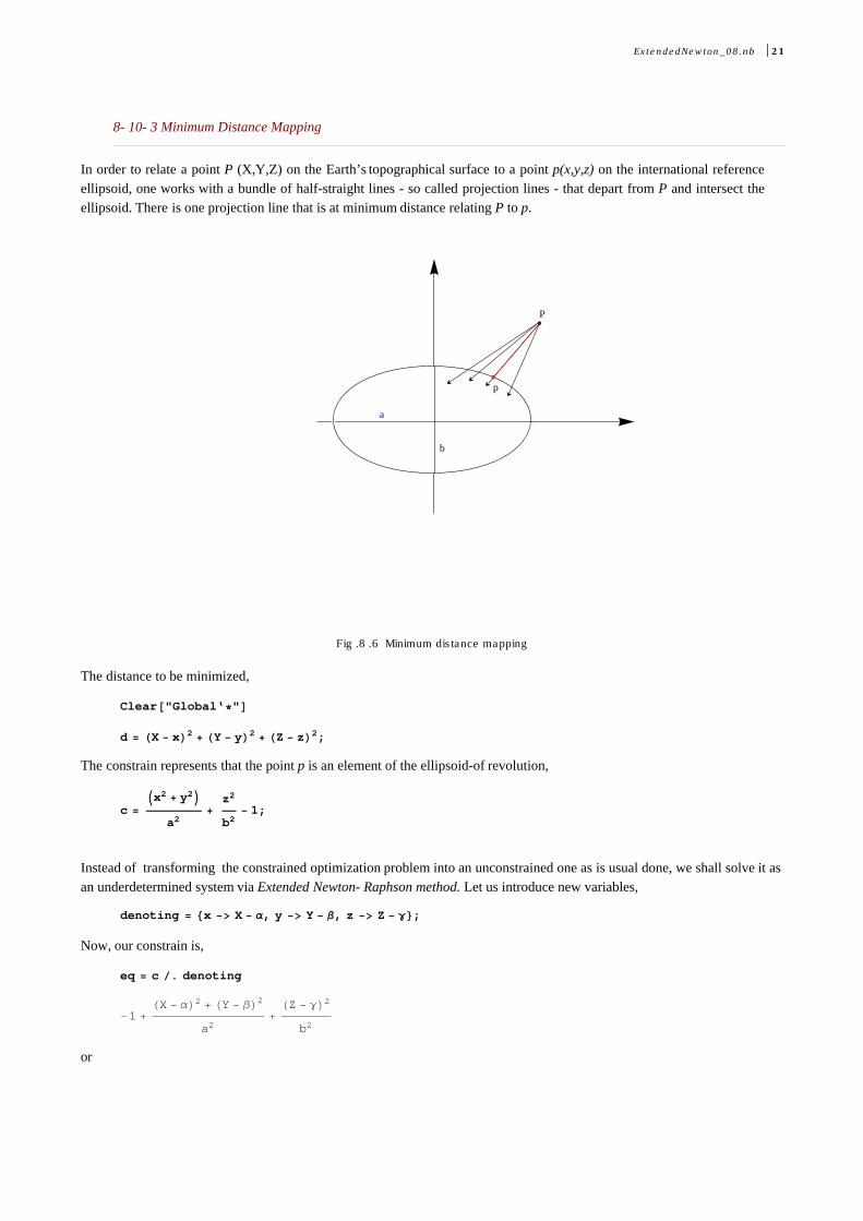
In order to relate a point P (X,Y,Z) on the Earth’s topographical surface to a point p(x,y,z) on the international referenceellipsoid, one works with a bundle of half-straight lines - so called projection lines - that depart from P and intersect theellipsoid. There is one projection line that is at minimum distance relating P to p.
P
p
a
b
Fig .8 .6 Minimum distance mapping
The distance to be minimized,
Clear@"Global‘*"D
d = HX - xL2 + HY - yL2 + HZ - zL2;
The constrain represents that the point p is an element of the ellipsoid-of revolution,
c =Ix2 + y2M
a2+
z2
b2- 1;
Instead of transforming the constrained optimization problem into an unconstrained one as is usual done, we shall solve it asan underdetermined system via Extended Newton- Raphson method. Let us introduce new variables,
denoting = 8x -> X - Α, y -> Y - Β, z -> Z - Γ<;
Now, our constrain is,
eq = c �. denoting
-1 +HX - ΑL2 + HY - ΒL2
a2+
HZ - ΓL2
b2
or
ExtendedNewton_08.nb 21
eq = eq a2 b2 �� Expand
-a2 b2 + b2 X2 + b2 Y2 + a2 Z2 - 2 b2 X Α + b2 Α2 - 2 b2 Y Β + b2 Β2 - 2 a2 Z Γ + a2 Γ2
The input data are the coordinates of the station Borkum (Germany), see text book,
data = 8X ® 3 770 667.9989, Y ® 446 076.4896,
Z ® 5 107 686.2085, a ® 6 378 136.602, b ® 6 356 751.860<;
Then our equation becomes in numerical form,
eqn = eq �. data
2.33091 ´ 1022 - 3.04733 ´ 1020 Α + 4.04083 ´ 1013 Α2 -
3.60504 ´ 1019 Β + 4.04083 ´ 1013 Β2 - 4.15568 ´ 1020 Γ + 4.06806 ´ 1013 Γ2
Let us normalize it,
eqn = eqn � eqn@@1DD �� Expand
1. - 0.0130735 Α + 1.73358 ´ 10-9Α2 -
0.00154662 Β + 1.73358 ´ 10-9Β2 - 0.0178286 Γ + 1.74527 ´ 10-9
Γ2
Now, we have a single equation with 3 variables (Α, Β, Γ). This underdetermined problem has infinite solutions. In order toselect the proper solution we seek a solution with minimal norm, since the distance to be minimized,
d = Α2 + Β2 + Γ2
A good initial guess is (Α, Β, Γ) = {0, 0, 0}. Let us employ Extended Newton-Raphson method,
sol = NewtonExtended@8eqn<, 8Α, Β, Γ<, 80., 0., 0.<, 10^-12, 100D �� Last
826.6174, 3.14888, 36.2985<
Returning back to the original variables,
8X - Α, Y - Β, Z - Γ< �. data �. 8Α ® sol@@1DD, Β ® sol@@2DD, Γ ® sol@@3DD<
93.77064 ´ 106, 446 073., 5.10765 ´ 106=
NumberForm@%, 15D
93.77064138151124 ´ 106, 446073.34071727, 5.10764991001691 ´ 106=
which is a quite precise solution, do compare it with the results in Chapter 18.
References
Bard Y. (1974) Nonlinear Parameter Estimation, Academic Press, New York.
Chapra S.C. and Canale R.P. (1998) Numerical Methods for Engineers, p. 159, 3rd Edition, McGraw-Hill, Boston.
Quoc - Nam Tran (1998) A Symbolic- Numerical Method for Finding a Real Solution of an Arbitrary System of NonlinearAlgebraic Equations, J. Symbolic Computation, 26, pp. 739- 760.
Ojika, T. (1987) Modified deflation algorithm for the solution of singular problems. I. A system of nonlinear algebraicequations. J.Math.Anal.Appl. 123., pp. 199 - 221
Ruskeepä ä H. (2009). Mathematical Navigator, 3rd Edition, Elsevier Academic Press, Amsterdam
22 ExtendedNewton_08.nb