Education Technology, Human CapitalDistribution and Growth

Jean-Marie ViaeneErasmus University, Tinbergen Institute and CESifo

Itzhak ZilchaThe Eitan Berglas School of Economics, Tel Aviv University‡

May 24, 2006

Abstract

The paper studies differences in education technology and theireffects on growth and on income distributions. Our overlapping gen-erations economy has the following features: (1) consumers are het-erogenous with respect to ability and parental human capital; (2) in-tergenerational transfers take place via parental education and, publicinvestments in education financed by taxes (possibly, with a level de-termined by majority voting); (3) due to investment in human capital,which is a factor of production, we have endogenous growth. Be-sides exploring several variations in the production of human capital,some attributed to ’home-education’ and others related to ’public-education’, we indicate how the level of public education can lead tonegative growth rates and affect the intragenerational income inequal-ity along the equilibrium path.JEL classification: D91; E25; H52Keywords: Human Capital; Innate Ability; Inequality Dynamics.

*We have received helpful comments from seminar participants at Athens(AUEB), Cyprus, Leuven, Rochester, Stockholm (IIES), the meeting of theEuropean Economic Association (Venice) and the conference on ”Extendingthe Tinbergen Heritage” (Rotterdam). This paper was partly written whilethe first author was visiting the Institute of International Economic Studies(IIES) at Stockholm University, whose hospitality and financial support aregratefully acknowledged. Research assistance by D. Ottens and E. Meesen isgratefully acknowledged.

1

‡Addresses for correspondence: J.-M. Viaene, Erasmus University, De-partment of Economics, H8-8, P.O. Box 1738, 3000 DR Rotterdam, TheNetherlands; Phone: +31-10-4081397; Fax: +31-10-4089161; E-mail: vi-aene@few.eur.nlI. Zilcha, The Eitan Berglas School of Economics, Tel-Aviv University,

Ramat Aviv, 69978 Israel; Phone: +972-3-640-9913; Fax: +972-3-640-9908;E-mail: izil@post.tau.ac.il

1 Introduction

Statistical offices of international organizations have compiled lists of indica-tors that compare scholastic achievements across countries. A primary com-mon element of these indicators is that the processes of training and knowl-edge acquisition differ in various parts of the world. Significant differencesbetween countries arise mainly in the following areas: the level and efficiencyof public education, involvement of parents in the education process of theirchildren, the human capital of teachers and the use of existing technologiessuch as computers and internet. Since human capital formation affects out-put and the intragenerational distribution of human capital, it is essential toexplore how these differences in the provision of education matter. In par-ticular, the purpose of this paper is to show how the education technologyaffects the distribution of earnings and the accumulation of human capitalin equilibrium.Though human capital formation is a complex process theoretical eco-

nomic models in the literature have assumed various restricted mechanismsgoverning this process. Due to tractability reasons, these processes haveconcentrated only on very few parameters [see, e.g., Glomm and Ravikumar(1992), Eckstein and Zilcha (1994), Laitner (1997), Orazem and Tesfatsion(1997) and Hanushek (2002)]. The implications of these simplifications re-garding the human capital production function are far reaching, since thedynamics of the human capital distribution is significantly affected. We shallconsider a human capital production process that exhibits two importantproperties. First, the importance of parental human capital in the process ofgenerating human capital of the offspring is well established in the literature[see, e.g., Hanushek (1986)]. Glaeser (1994) finds that children from familieswith educated parents obtain better education. Burnhill et al. (1990) findthat parental education influences entry into higher education in Scotlandover and above parental social status. Lee and Barro (2001) and Brunelloand Checchi (2003) find that family characteristics, such as income and ed-ucation of parents, enhance student’s performance. A reason that is put

2

forward is that parental education elicits more parental involvement (includ-ing related private investment) at home. Second, the contribution of publiceducation to human capital formation depends on both the level of provisionand the quality of teachers. Individuals from below-average human capitalfamilies will have a greater return to investment in public schooling thanthose from above-average families. In addition, the cost of acquiring humancapital will be smaller for societies endowed with relatively higher levels ofaverage human capital [see, e.g., Tamura (1991), Fischer and Serra (1996)].Our analysis is conducted in an OLG economy in which physical capital

and human capital are factors of production. In each generation we obtainheterogeneity due to the human capital distribution of the parents, as wellas individual’s (random) innate ability. Education and learning take placevia two channels: the time invested by parents at home educating their child(motivated by altruism) and the provision of public education financed bytaxing wage incomes. Home education is carried out mainly through parentaltutoring, social interaction and the learning devices available at home (suchas computor and internet). In this case the human capital of parents and thetime dedicated to tutoring are important factors. Public education includespublic expenditures related to schooling, in particular, the time childeren arestudying in school, as well as the quality of teachers, size of classes, ’outside’social interactions, etc. Our framework will generate endogenous growth inhuman capital, due to investments in education and training, and will allowfor a political equilibrium regarding the provision of public education (usingthe median-voter theorem). We derive the following results in competitiveequilibrium: (i) Public education reduces income inequality: more provisionof public schooling reduces inequality in the distribution of human capital.Moreover, if the investment in public education is ’too low’ the stock of hu-man capital may decline over time. (ii) Initial endowments matter in thesense that a country starting from a lower level of human capital has a lowerreturn to public education and, hence, experiences more inequality. Further-more, international trade in goods and physical capital mobility, based onthese endowment differences, do not alter the autarky income inequality. (iii)When the provision of public education becomes more efficient intragener-ational income inequality declines in all subsequent periods. If the privateprovision of education becomes more efficient instead income inequality in-creases in all subsequent periods. Thus, there is a basic asymmetry in theeffects of technological change in the two types of provision on income in-equality. (iv) If the level of provision of public education is determined bymajority voting our results are strengthened.The remainder of the paper is organized as follows. The next section ex-

amines the literature. Section 3 presents an OLG model with heterogeneous

3

agents and analyzes the properties of this framework. Section 4 studies theeffects of variations in the education technology on intragenerational incomeinequality. Section 5 concludes the paper. We shall relegate the proofs to anAppendix, to facilitate the reading.

2 Related Literature

Income distribution is a key economic issue and a large literature has im-proved our understanding of its underlying determinants. Besides trade andtechnical progress, some believe that social norms are crucial determinantsof earnings inequality [e.g., Atkinson (1999), Corneo and Jeanne (2001)].Others have thoroughly studied the role of human capital accumulation onincome distribution in various contexts [see, e.g., Loury (1981), Becker andTomes (1986), Galor and Zeira (1993), Benabou (1996), Chiu (1998), Fernan-dez and Rogerson (1998)]. However, as the information and communicationtechnology advances and computors are being integrated into the learningprocess, new issues like the increasing technological contribution to learningarise. These technological changes, which strongly differ across countries, areanalyzed in Section 4.The literature also contains work on how education systems come about.

For example, Glomm and Ravikumar (1992) establish that majority votingresults in a public educational system as long as the income distribution isnegatively skewed. Cardak (1999) strengthens this result by considering avoting mechanism where the median preference for education expenditure,rather than median income household, is the decisive voter. The equilibriumwe consider in Section 4 is an application of the median-voter theorem. Weshow that majority voting strengthens the results regarding income inequalityobtained under exogenous tax rates.As was demonstrated in various ways, endogenous growth models provide

an efficient analytical tool in studying issues related to growth, convergenceand income inequality in equilibrium [see, e.g., Loury (1981), Tamura (1991),Glomm and Ravikumar (1992), Fischer and Serra (1996), Fernandez andRogerson (1998), van Marrewijk (1999), Galor and Moav (2000), Viaene andZilcha (2002, 2003)].1 The main emphasis has been on the role played by

1This paper is related to Viaene and Zilcha (2003) but the model differs in two mainrespects. (1) Each individual has now a random innate ability to learn. This innate abilityturns out to be crucial for some theoretical results, in particular regarding individual util-ity. (2) This paper incorporates the corner solutions that arise from the non-participationof parents to the education achievements of their younger generation.

4

human capital as an engine for growth [see, e.g., Razin (1973), Lucas (1988),Azariadis and Drazen (1990)]. Our model in the stationary state is an AK-model where all variables grow at the same rate as effective labor. However,we consider only non-stationary competitive equilibria.The concepts of growth and income inequality are inter-woven. The well-

documented literature on the growth performance of countries has tried tosubstantiate a negative relationship between inequality and growth. Earlytests of this hypothesis by Alesina and Rodrick (1994), Persson and Tabellini(1994) and others report evidence of an inverse relationship, while more re-cent empirical findings, for instance, by Barro (2000) and Forbes (2000),suggest a positive relationship instead. As in the empirical literature ourwork takes no explicit stance regarding the causality between inequality andgrowth. Basically, we point out that the way in which countries enhancehuman capital matters: If the gap between countries is mainly in the ’home’component of human capital formation it results in higher growth while in-come inequality rises. In contrast, when this gap occurs in the ’public’ part,then higher growth is accompanied by less income inequality.

3 The Model

3.1 Human Capital Formation

Consider an overlapping generations economy with a continuum of consumersin each generation, each living for three periods. During the first period eachchild is engaged in education/training, but takes no economic decision. Indi-viduals are economically active during the working period which is followedby the retirement period. We assume no population growth, hence popula-tion is normalized to unity. At the beginning of the ’working period’, eachparent gives birth to one offspring. Each household is characterized by a fam-ily name ω ∈ [0, 1]. Denote by Ω = [0, 1] the set of families in each generationand by µ the Lebesgue measure on Ω.Agents are endowed with two units of time in their second period. One

unit is inelastically supplied to labor, while the other is allocated betweenleisure and self-educating the offspring.2 Consider generation t, denoted Gt,namely all individuals ω born at the outset of date t−1, and let ht(ω) be thelevel of human capital of ω ∈ Gt.We assume that the production function for

2Though the supply of labor is inelastic, each family’s supply of human capital isthe result of utility maximization. Due to our assumption of no population growth, theassumption of an inelastic labor supply is less severe since the time required to raisechildren is equal at each date and is insensitive to the number of young-age children.

5

human capital is composed of two components: informal education initiatedand provided by parents at home and public education provided by the gov-ernment by hiring ’teachers’, constructing schools etc. The ’home-education’depends on the time allocated by the parents to this purpose, denoted byet(ω), and the ’quality of tutoring’ represented by the parent’s human capitallevel ht(ω). The time allocated to public schooling (i.e., the level of publiceducation) is denoted by egt. The human capital of the teachers determinethe ’quality’ of public education in the formation of the younger generation’shuman capital. We also assume that the (random) innate ability of individ-ual ω ∈ Gt+1, denoted by θt(ω), is known when parents make their decisionabout investment in education. Moreover, all the random variables θt(ω)across individuals and across generations are i.i.d., hence, without loss ofgenerality, we take each θt(ω) to be distributed as some random variable eθ.Let eθ assume values in [θ, θ], where 0 < θ < θ <∞, and denote its mean by bθwhere, without loss of generality, bθ = 1.We assume that for some parametersβ1 > 1, β2 > 1, υ > 0 and η > 0, the evolution process of a family’s humancapital is given as follows. For all ω ∈ Gt+1 :

ht+1(ω) = θt(ω)[β1et(ω)hυt (ω) + β2egth

η

t ] (1)

where the human capital involved in public schooling, denoted ht, is theaverage human capital of generation t. This is justified if we assume that in-structors in each generation are chosen randomly from the population of thatgeneration. The parameters υ and η measure the externalities derived fromparents’ and society’s human capital respectively. The constants β1 and β2represent how efficiently parental and public education contribute to humancapital: β1 is affected by the home environment while β2 is affected by facil-ities, the schooling system, size of classes, neighborhood, social interactions,and so forth3.The production function for human capital given by (1) exhibits the prop-

erty that public education dampens the family attributes. As it is common toall, individuals from below-average families have, therefore, a greater returnto human capital derived from public schooling than those born to above-average human capital families. In addition, the effort of acquiring human

3Empirical support for (1) is abundant, but let us point out to Brunello and Checchi(2003) who demonstrate, using Italian data, the importance of both ’home’ and ’public’education in human capital formation. The family background in human capital formationhas been shown to be empirically significant in the case of East Asia by Woessmann (2003).Card and Krueger (1992) established, using US data, that differences in school qualitymatters when we consider the rate of return to education. A lower pupil/teacher ratioresults in a higher return.

6

capital is smaller in countries endowed with relatively higher levels of hu-man capital. An important difference between our process of human capitalacquisition and most cases discussed in the literature is the representationof the private and the public inputs in the production of human capital viaallocation of time.4 Our approach assumes that the time spent learning, cou-pled with the human capital of the instructors, and not the expenditures oneducation, should be the relevant variables in such a process although theremay exist a relationship between the quality of public education and publicexpenditure on education.5.Consider the lifetime income of individual ω, denoted by yt(ω). Since the

human capital of a worker is observable, it depends on the effective laborsupply. Let wt be the wage rate in period t and τ t is the tax rate on laborincome, then:

yt(ω) = wt(1− τ t)ht(ω) (2)

Under the public education regime the taxes on incomes are used to financeeducation costs of the young generation. Making use of (1) and (2), balancedgovernment budget means:Z

Ω

wtegthtdµ(ω) =

ZΩ

τ twtht(ω)dµ(ω)

or equivalently,egt = τ t (3)

that is, the tax rate on labor is equal to the proportion of the economy’seffective labor used for public education.6

4Home and public education play different roles in the literature. For example, inEckstein and Zilcha (1994) there is investment in home education on the part of parentsin terms of time. In Eicher (1996), young agents must decide whether to enter the privateeducation sector as students or to work in production as unskilled workers. In Orazem andTesfatsion (1997), there is private investment in terms of effort and in Viaene and Zilcha(2002) there is a time input for public education only. In Restuccia and Urrutia (2004),children in their first period of life acquire human capital through public education financedby income taxes and through private education via additional personal expenditures.

5This is in line with Hanushek (2002) who argues in favor of considering the ’efficiency’in the public education provision rather than ’expenditure’ on public education. Thisdistinction is important since in a dynamic framework the cost of financing a particularlevel of human capital fluctuates with relative factor rewards.

6 Under a decentralized system, namely under a fully private education regime, bothτ t(ω) and egt(ω) are decision variables of each agent, hence the individual’s budget con-straint on private education is: τ t(ω)wtht(ω) = wtegt(ω)ht, where the level of teachers’instruction egt(ω) is chosen freely while their average human capital is the same as theircorresponding generation.

7

3.2 Equilibrium

Production in this economy is carried out by competitive firms that producea single commodity, using effective labor and physical capital. This com-modity is both consumed and used as production input. Physical capitalfully depreciates and the per-capita effective human capital in date t, ht,is an input in aggregate production. In particular we take the (per-capita)production function to be:

qt = F (kt, (1− egt)ht) (4)

where kt is the capital stock and (1 − egt)ht = (1 − τ t)ht is the effec-tive human capital used in the production process. F(·,·) is assumed toexhibit constant returns to scale; it is strictly increasing, concave, contin-uously differentiable and satisfies Fk(0, (1 − τ t)ht) = ∞, Fh(kt, 0) = ∞,F (0, (1− τ t)ht) = F (kt, 0) = 0.

Given the public education provision, agent ω at time tmaximizes lifetimeutility, which depends on consumption, leisure and income of the offspring.Thus:

maxet,st

ut(ω) = c1t(ω)α1c2t(ω)

α2yt+1(ω)a3 [1− et(ω)]

α4 (5)

subject toc1t(ω) = yt(ω)− st(ω) ≥ 0 (6)

c2t(ω) = (1 + rt+1)st(ω) (7)

where ht+1(ω) and yt+1(ω) are given by (1) and (2). The α0is are knownparameters and αi > 0 for i = 1, 2, 3, 4; c1t(ω) and c2t(ω) denote, respectively,consumption in first and second period of the individual’s economically activelife; st(ω) represents savings; leisure is given by (1 − et(ω)); (1 + rt+1) isthe interest factor at date t. The offspring’s income yt+1(ω) enters parents’preferences directly and represents the motivation for parents’ investment intutoring and formal education expenditure. Given some tax rates (τ t), k0 andthe initial distribution of human capital h0(ω), a competitive equilibrium iset(ω), st(ω), kt;wt, rt which satisfies: For all t and all individuals ω ∈ Gt ,et(ω), st(ω) are the optimum to the above problem given wt, rt. And,the following market clearing conditions hold:

wt = Fh(kt, (1− egt)ht) (8)

(1 + rt) = Fk(kt, (1− egt)ht) (9)

8

kt+1 =

ZΩ

st(ω)dµ(ω) (10)

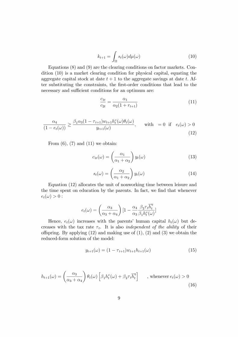
Equations (8) and (9) are the clearing conditions on factor markets. Con-dition (10) is a market clearing condition for physical capital, equating theaggregate capital stock at date t+ 1 to the aggregate savings at date t. Af-ter substituting the constraints, the first-order conditions that lead to thenecessary and sufficient conditions for an optimum are:

c1tc2t=

α1α2(1 + rt+1)

(11)

α4(1− et(ω))

≥ β1α3(1− τ t+1)wt+1hυt (ω)θt(ω)

yt+1(ω), with = 0 if et(ω) > 0

(12)

From (6), (7) and (11) we obtain:

c1t(ω) =

µα1

α1 + α2

¶yt(ω) (13)

st(ω) =

µα2

α1 + α2

¶yt(ω) (14)

Equation (12) allocates the unit of nonworking time between leisure andthe time spent on education by the parents. In fact, we find that wheneveret(ω) > 0 :

et(ω) =

µα3

α3 + α4

¶[1− α4

α3

β2τ thη

t

β1hυt (ω)

]

Hence, et(ω) increases with the parents’ human capital ht(ω) but de-creases with the tax rate τ t. It is also independent of the ability of theiroffspring. By applying (12) and making use of (1), (2) and (3) we obtain thereduced-form solution of the model:

yt+1(ω) = (1− τ t+1)wt+1ht+1(ω) (15)

ht+1(ω) =

µα3

α3 + α4

¶θt(ω)

hβ1h

υt (ω) + β2τ th

η

t

i, whenever et(ω) > 0

(16)

9

ht+1(ω) = β2θt(ω)τ thη

t , whenever et(ω) = 0 (17)

Equations (15)-(17) determine the income at the future date in terms ofthe net wage at date t+1, the parents’ human capital, society’s level of humancapital at date t, the current education input (τ t = egt) and the externalitiesin education. More importantly, (15) shows that, in our framework, theintragenerational distribution of income of any date is similar to that ofhuman capital.

3.3 Non-participation of Parents

The non-participation of parents in the education process is an importantcharacteristic of education systems in some OECD countries like Germany.7

This situation, where utility maximization is attained at et(ω) = 0, occursunder certain conditions. To derive these recall that (12) establishes a nega-tive relationship between the two types of education, that is, public educationsubstitutes for parental tutoring. For each individual there exists a particulartax rate such that et(ω) = 0, namely, when the marginal utility of leisureis larger than the utility gain obtained from a marginal increase in the off-spring’s human capital due to parental tutoring. Consider the families whichoptimally choose et(ω) = 0 and denote this set of families in generation t byAt ⊂ Gt = [0, 1]. In fact, condition (12) holds if:

1− et(ω) <α4β1α3

[β1et(ω) + β2egthη

t

hυt (ω)]

Hence, for each individual in Gt we obtain et(ω) = 0 and ω ∈ At if :

hυt (ω) <α4β2egtα3β1

hη

t (18)

Parental and public education being substitutes, inequality (18) shows thatthe set At increases as the provision of public education egt increases. It isclear that this set includes individuals with low levels of human capital.

7See, e.g., Der Spiegel (2001) and DICE Reports (2002) for attempts at explainingthe poor performance of German adolescents in the 2000 study of the Programme forInternational Student Assessment (PISA) of the OECD.

10

3.4 Under-provision of Public Education

As parental education is crowded out by public schooling, let us examine thenet contribution of public education to the long-run human capital stock. Tosimplify our analysis we assume, in this section only, a stationary provision ofpublic education, i.e., egt = eg = τ for all t. Let us impose some restrictionson the parameters in our economy in order to demonstrate the following: Thelevel of public education is critical to the positive or negative accumulationof human capital. We assume in this section only that the parameters in oureconomy satisfy the following conditions:(A1) α3β1

α3+α4< 1− ξ, for some ξ > 0 .

(A2) The initial distribution h0(ω) satisfies: h0 ≥ 1 .(A3) η = 1 and υ = 1.(A4) α4 > α3.

Proposition 1 Assume that (A1) - (A4) hold. Then:(a) If eg satisfies:

eg ≤ [1− α3β1α3 + α4

]β−12 (19)

then, along the equilibrium path, the aggregate human capital decreases,

namely, ht+1 < ht for t = 0, 1, 2, ......(b) If eg satisfies:

eg ≥ [1− α3β1α3 + α4

]α3 + α4α3β2

(20)

then the aggregate human capital increases, i.e., ht+1 > ht for all t.This result underlines the important role played by the level of public

education. To emphasize this point, let us compare two countries whichdiffer in the provision of public education and in their initial distributions ofhuman capital, given that each economy satisfies (A1)-(A4). If eg is chosen tobe low in one country, assuming that condition (19) holds, while in the othercountry it is higher, say condition (20) holds, then we obtain negative growthin the former country while the latter has a positive rate of growth. Evidenceof countries with declining human capital can be found at the World Banksite even though the reasons for a declining human capital might be otherthan the ones discussed here, such as AIDS epidemic, wars or oppressiveregimes. Also, both conditions (19) and (20) can be tested on the basis ofknown parameters for the utility function and the learning technology.

11

3.5 Endogenous Growth

Consider the competitive equilibria for some given initial conditions and com-pare the long run properties of this economy under the various regimes ofeducation we have considered. Define the growth factor of aggregate laborsupply as:

γt ≡∫Ω ht+1(ω)dµ(ω)∫Ω ht(ω)dµ(ω)

(21)

Since, by our assumptions, ability θt(ω) is independent of ht(ω) and hυt (ω),substituting (16) in (21) gives rise to an alternative expression for γt :

γt =

µα3

α3 + α4

¶·β1∫Ω hυt (ω)dµ(ω)∫Ω ht(ω)dµ(ω)

+ β2τ thη−1t

¸(22)

The growth rate is positive as long as (22) is greater than 1. The twoterms in the square brackets represent the two channels through which incomedistribution can matter for the growth factor of aggregate labor: (1) viaparental education and (2) via the endogenous determination of τ t like in amedian-voter equilibrium. If education has constant returns to scale [hence,ν = η = 1], then:

γt =α3

α3 + α4[β1 + β2τ t] (23)

The growth factor γt is larger than unity for β1 and β2 sufficiently large.The following monotonicity results can be verified:

∂γt∂α3

> 0 and∂γt∂α4

< 0 ,∂γt∂β1

> 0,∂γt∂β2

> 0 (24)

It is clear from (23) that the time independence of τ t implies time inde-pendence of γ as well. In addition, when we take the aggregate productionfunction to be Cobb-Douglas, then by direct computation we obtain that:qt+1/qt = γ. In the stationary state our model is then an AK-type endoge-nous growth model where all variables grow at the rate (γ − 1).

4 Income Distribution

The objective of this section is to consider changes in the intragenerationalincome distribution, in equilibrium, due to variations in education systems.

12

Such variations can be attributed to numerous factors but the ones con-sidered here reflect cross-country differences in the process describing theaccumulation of human capital. This section deals mainly with differences inlevels of public education, differences in education technology and in factorendowments. We use second degree stochastic dominance to rank inequality[see Atkinson (1970)].

4.1 The Role of Initial Endowments

To show why initial conditions matter consider two economies that differ onlyin their initial endowments of human capital: one economy has higher levelsof human capital but the measure of inequality in the initial human capitaldistributions is the same. The next proposition compares the equilibriumpath of these two countries.

Proposition 2 (Inequality: the Endowment Effect) Consider two economieswhich differ only in their initial human capital distributions, h0(ω) and h∗0(ω).Assume that h∗0(ω) > h0(ω) for all ω, but the initial distributions have thesame level of inequality. Then, the equilibrium from h∗0(ω) will have lowerincome inequality than that from h0(ω) at all dates.

Thus the initial distribution of human capital matters: a country thatstarts with higher levels of human capital, not necessarily more equal, has ahigher return to public education and, hence, has a better chance to main-tain less inequality in its future income distributions. Given the differentendowments of human capital it is possible to introduce international tradeand mobility of physical capital between these two economies, keeping laborimmobile internationally. These assumptions about trade and factor mobil-ity guarantee factor price equalization. In this setting, we can show thatif initial endowments of human capital (or physical capital) differ betweencountries then opening markets does not affect our results regarding incomeinequality.

Proposition 3 (Inequality: International Trade Effect) Consider twoeconomies which differ in their initial conditions. Trade in goods and capitalmobility do not alter the income inequality observed under autarky.

Variations in the equilibrium factor prices do not affect our results re-garding income inequality since labor incomes vary in the same proportion.

13

Hence, trade plays no role in explaining intragenerational income inequal-ity in our framework, which provides a justification for our approach thatconsists in comparing countries’ education systems separately. In contrast,trade and capital mobility has a significant impact on wages, interest ratesand outputs of any two countries and, in this regard, affects the intergen-erational distribution of income along the lines shown in the literature [see,e.g.,Viaene and Zilcha (2002)].

4.2 The Role of Public Education

Let us consider first a situation in which the government does not contributeto human capital formation. Thus, we take τ t = 0 for all t. In this case:

yt+1(ω) = wt+1ht+1(ω)

From (18) we know that the set At is empty, and from (12) we obtainthat:

et(ω) = e∗(ω) =α3

α3 + α4for all ω

We see that in that absence of public education the only source of incomeinequality is the initial distribution of human capital. This is clear from:

yt+1(ω) = [β1wt+1e∗hvt (ω)]θt(ω)

We conclude from these observations that:

Proposition 4 In the absence of public education income inequality (i) declinesover time under decreasing returns to parental human capital (i.e., if v < 1),(ii) increases over time under increasing returns (i.e., if v > 1), and (iii)remains constant over time under constant returns (i.e., if v = 1).

Our economy generates, in equilibrium, an intragenerational income dis-tribution whose inequality is endogenously determined by the externality inthe home-part of education. Inequality may decrease even in the absence ofpublic schooling. When v > 1 a family ’poverty trap’ arises in that ht(ω)goes to zero for some families whose initial endowment of human capital isbelow a benchmark level. More precisely, this occurs for family ω such that:

h0(ω) < [α3 + α4

β1α3θ0h0(ω)]

1v−1

14

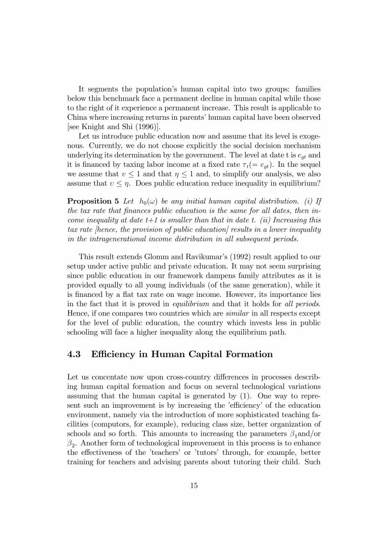
It segments the population’s human capital into two groups: familiesbelow this benchmark face a permanent decline in human capital while thoseto the right of it experience a permanent increase. This result is applicable toChina where increasing returns in parents’ human capital have been observed[see Knight and Shi (1996)].Let us introduce public education now and assume that its level is exoge-

nous. Currently, we do not choose explicitly the social decision mechanismunderlying its determination by the government. The level at date t is egt andit is financed by taxing labor income at a fixed rate τ t(= egt). In the sequelwe assume that v ≤ 1 and that η ≤ 1 and, to simplify our analysis, we alsoassume that υ ≤ η. Does public education reduce inequality in equilibrium?

Proposition 5 Let h0(ω) be any initial human capital distribution. (i) Ifthe tax rate that finances public education is the same for all dates, then in-come inequality at date t+1 is smaller than that in date t. (ii) Increasing thistax rate [hence, the provision of public education] results in a lower inequalityin the intragenerational income distribution in all subsequent periods.

This result extends Glomm and Ravikumar’s (1992) result applied to oursetup under active public and private education. It may not seem surprisingsince public education in our framework dampens family attributes as it isprovided equally to all young individuals (of the same generation), while itis financed by a flat tax rate on wage income. However, its importance liesin the fact that it is proved in equilibrium and that it holds for all periods.Hence, if one compares two countries which are similar in all respects exceptfor the level of public education, the country which invests less in publicschooling will face a higher inequality along the equilibrium path.

4.3 Efficiency in Human Capital Formation

Let us concentate now upon cross-country differences in processes describ-ing human capital formation and focus on several technological variationsassuming that the human capital is generated by (1). One way to repre-sent such an improvement is by increasing the ’efficiency’ of the educationenvironment, namely via the introduction of more sophisticated teaching fa-cilities (computors, for example), reducing class size, better organization ofschools and so forth. This amounts to increasing the parameters β1and/orβ2. Another form of technological improvement in this process is to enhancethe effectiveness of the ’teachers’ or ’tutors’ through, for example, bettertraining for teachers and advising parents about tutoring their child. Such

15

an improvement amounts to increasing the parameters v and η, that bringinto expression the effectiveness of the human capital of the parents and/orthat of the ’teachers’. We assume that v ≤ 1 and η ≤ 1 in the sequel, eventhough this assumption can be relaxed in most cases8.An improvement in one country (vs. the other) in the production of hu-

man capital may result in a more efficient home education or a more efficientpublic education, or both. We say that the provision of public education ismore efficient if either β2/β1 is larger (without lowering neither β1 nor β2) orη is larger, or both. We say that the private provision of education becomesmore efficient if β1/β2 becomes larger (while neither β1 nor β2 declines) or νbecomes larger, or both. It is called neutral in the case where both parame-ters β1 and β2 increase while the ratio β2/β1 remains unchanged. The nextproposition, which contains the main result of the paper, considers the effectof each type of technological gap on intragenerational income inequality.

Proposition 6 Consider improvements in the production process of humancapital, then: (a) If the public provision of education becomes more efficientthe inequality in intragenerational distribution of income declines in all pe-riods; (b) If the private provision of education becomes more efficient theninequality increases in all periods; (c) If the technological improvement isneutral inequality remains unchanged at period 1 but declines for all periodsafterwards.

This result demonstrates the asymmetry between a technological gap thatexists primarily in the public schooling system and the one that arises in thehome environment of learning. The inequality in human capital distributionincreases when the private-component of education/learning becomes moreefficient because the family attributes are magnified. In contrast, a moreefficient public education reduces inequality because all children are exposedto instructors with the same average level of human capital: below-averagefamilies have a greater return to public schooling than above-average fam-ilies. When the technological gap in education is neutral, then along the’better’ equilibrium inequality declines, except for the first date, since, afterthe first period, the effectiveness of public schooling outweighs that of homeeducation.

Median-Voter Equilibrium8Throughout this paper we ignore the effect of technological change in the aggregate

production function upon inequality. The reason is that even though such changes affectlabor income it does not affect inequality in income distribution, since all incomes arevaried in the same proportion.

16

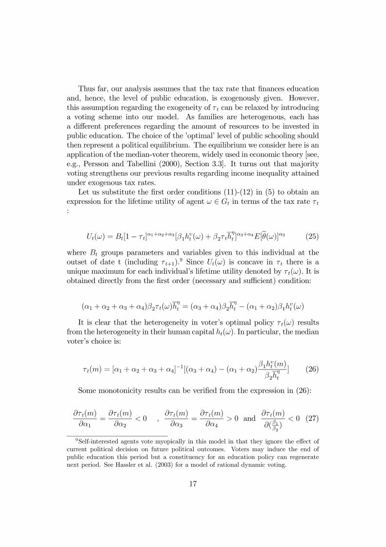
Thus far, our analysis assumes that the tax rate that finances educationand, hence, the level of public education, is exogenously given. However,this assumption regarding the exogeneity of τ t can be relaxed by introducinga voting scheme into our model. As families are heterogenous, each hasa different preferences regarding the amount of resources to be invested inpublic education. The choice of the ’optimal’ level of public schooling shouldthen represent a political equilibrium. The equilibrium we consider here is anapplication of the median-voter theorem, widely used in economic theory [see,e.g., Persson and Tabellini (2000), Section 3.3]. It turns out that majorityvoting strengthens our previous results regarding income inequality attainedunder exogenous tax rates.Let us substitute the first order conditions (11)-(12) in (5) to obtain an

expression for the lifetime utility of agent ω ∈ Gt in terms of the tax rate τ t:

Ut(ω) = Bt[1− τ t]α1+α2+α3[β1h

υt (ω) + β2τ th

η

t ]α3+α4E[eθ(ω)]α3 (25)

where Bt groups parameters and variables given to this individual at theoutset of date t (including τ t+1).

9 Since Ut(ω) is concave in τ t there is aunique maximum for each individual’s lifetime utility denoted by τ t(ω). It isobtained directly from the first order (necessary and sufficient) condition:

(α1 + α2 + α3 + α4)β2τ t(ω)hη

t = (α3 + α4)β2hη

t − (α1 + α2)β1hυt (ω)

It is clear that the heterogeneity in voter’s optimal policy τ t(ω) resultsfrom the heterogeneity in their human capital ht(ω). In particular, the medianvoter’s choice is:

τ t(m) = [α1 + α2 + α3 + α4]−1[(α3 + α4)− (α1 + α2)

β1hυt (m)

β2hη

t

] (26)

Some monotonicity results can be verified from the expression in (26):

∂τ t(m)

∂α1=

∂τ t(m)

∂α2< 0 ,

∂τ t(m)

∂α3=

∂τ t(m)

∂α4> 0 and

∂τ t(m)

∂(β1β2)

< 0 (27)

9Self-interested agents vote myopically in this model in that they ignore the effect ofcurrent political decision on future political outcomes. Voters may induce the end ofpublic education this period but a constituency for an education policy can regeneratenext period. See Hassler et al. (2003) for a model of rational dynamic voting.

17

Observed cross-country differences in education expenditures can be ex-plained by (26) and (27). For example, as ht(m) drops relative to ht, τ t(m)rises: A below-average median voter favors a higher tax rate than an above-average median voter. Also, an increase in υ and β1/β2 [or a decrease in η]imply a lower tax rate for financing education.Given this, let us illustrate how majority voting strengthens our previous

results regarding income inequality. To show that, consider Propositions5 and 6 when β1 increases. This results in more inequality according toProposition 6. In addition, following this increase in β1 majority votingimplies a lower tax rate τ t(m), which by Proposition 5 leads to even moreinequality.

4.4 Inequality and Growth

In our framework the economy has no other source of income besides the onegenerated by the aggregate production in which human and physical capitalare used. Thus educational investments are essential to creating growth. Letus consider the growth-inequality relationship issue in our framework andthe causality linking them. To that end, we wish to compare two countrieswhich differ in some parameters of the human capital formation process. Asin the empirical literature it turns out that there is no explicit stance on thecausality between inequality and growth.Let us consider first the effect that a technological change in the produc-

tion of human capital has on output in equilibrium. Consider (1) and notethat we call the first term on the RHS, β1et(ω)h

υt (ω), the home-component,

and the second term, β2egthη

t , the public-component. An improvement in theproduction of human capital which makes either the public provision moreefficient or the private provision more efficient results in higher output atall dates. Any improvement, either in the public-component or the home-component, implies higher human capital stock as of period 1 and on. Since,the initial capital stock is given, this increases output in date 1 and, hence,aggregate savings in this period. Thus, output in date 2 is higher and hencethe capital stock to be used as well. Does a technological progress, which re-sults in higher growth, also mean less inequality? Let us combine our resultsto obtain:

Proposition 7 Consider some technological differences in the productionprocess of human capital, then: (a) If the technological gap occurs in thehome-component, it results in higher growth coupled with more income in-equality at all dates; (b) When the technological gap occurs in the public-component, it results in higher growth accompanied by less inequality.

18

The proof of this result is omitted as it follows directly from Proposition6. The issue of co-movements of economic growth and income inequality hasbeen widely debated in the literature, mainly by using empirical evidence,and this debate is inconclusive [see e.g., Persson and Tabellini (1994), Barro(2000) and Forbes (2000)]. Proposition 7 provides a theoretical frameworkthat helps us interpret these empirical findings. It establishes conditionsunder which higher growth is accompanied by more or less inequality asboth growth and inequality are endogenous variables. Their co-movementwill depend upon how they are related to the underlying shocks to whichthey respond.

A direct application of this proposition is to interpret the informationand communication technology (ICT) revolution, seen as a technological im-provement that enhances knowledge. According to the World Bank (2001,Table 19), the diffusion of information technology across countries is highlyuneven. The 1998 figures on the number of computers per 1000 people rangebetween 458.6 in the US and 0.2 in Niger. A more comprehensive ranking bythe ITU measures, besides availabilty, also the innate and financial abilitiesof individuals to use ICT [International Telecommunication Union (2003)].A similar gap has been observed in this case as well where Niger is rankedat the bottom but the US is positioned now as 11th. These observationsraise the following question: does the home component of human capitalformation benefit more than the public education component from the ICTrevolution? We believe that this is the case for two reasons. First, in manycountries computers and internet access have enhanced home education con-siderably, while public schools benefited in a lesser extent. Second, withincountries there are wide gaps between the have and have-not. Also, the useof the ICT raises the issues of affordability and education that emphasizethe importance of families’ human capital. In terms of our model, the firstargument means a rise in β1 that is proportionately larger than the rise in β2, while the second means an increase in ν. Both changes in these parametersincrease income inequality, in our framework, and imply higher growth.By the same reasoning part (a) of Proposition 7 may provide some expla-

nation to the recent observation (mostly during the last decade) that in mostOECD countries economic growth has been accompanied by higher incomeinequality.

19

5 Conclusion

This paper is one of the first attempts to study, within a general equilib-rium framework, the cross-country differences in income distribution. Ourframework of analysis is an overlapping-generations economy with heteroge-nous households, where heterogeneity results from random innate abilitiesand the nondegenerate initial distribution of human capital across individu-als. We derived a number of results which provide explanations for observedcross-country differences in income inequality based on different processesof human capital formation. In particular, our results suggest hypothesesregarding a cross-country comparison of inequality and : (a) externalitiesof family’s (and society’s) human capital; (b) the effective level of publiceducation; (c) the efficiency of public schooling and parental tutoring; (d)economic growth; (e) initial conditions, represented here by the initial stockof physical capital and the initial level and distribution of human capital; (f)the international environment, such as trade and physical capital mobility.

The paper illustrates the role of family attributes in the formation of hu-man capital. Any education system that emphasizes the role of a family, suchas private education, would lead to increased income inequality. Alternativemodels that would include the financing of private education would magnifythe results on income inequality.Our framework makes some specific assumptions and is therefore subject

to the issue of robustness. First, the selection of our functional forms wasstrongly motivated by stylized facts. For example, incorporating parentalrole in the human capital formation process is justified due to the repeatedlyreported evidence that it has an empirical relevance in a large number ofcountries. Second, each agent in our model supplies one unit of his time tothe labor market. The effect of relaxing the assumption of inelastic laborsupply is not trivial as each family’s supply of human capital is also endoge-nous. Moreover, due to zero population growth, our assumption seems lesssevere as the time required to raise children is equal at each date. Third,the model assumes away taxation of the returns to savings but expandingthe tax base to include this type of tax does not alter the results concerningincome inequality. In contrast, this framework can be generalized to includean additional redistributive measure by the government, such as social secu-rity. Some of our results may vary in this situation because intergenerationaltransfers take place via both education and social security.

20

6 Appendix

Before we prove our Propositions let us bring the following Lemma.Lemma: Let X(ω) and Y (ω) be two non-negative random variables

which assume values in a compact interval [a, b] and satisfy: EX = EY. LetZ(ω) be a positive random variable independent of X and Y . If X(ω) ismore equal than Y (ω) (in the SDSD sense), then XZ is more equal thanY Z.

Proof of the Lemma: Denote the cumulative distribution functions ofX,Y,Z by F (ξ), G(ξ) and H(ξ) correspondingly. Let [α, β] be the supportof Z. Define,

W (m) = PrXZ ≤ m = PrZ = ρ and X ≤ m

ρ, ρ ∈ [α, β]

It is clear that W (m) =R βαF (m

ρ)H(ρ)dρ. In the same way we define the

c.d.f of Y Z as W ∗(m) =R βαG(m

ρ)H(ρ)dρ. Let the support of W and W ∗ be

[c, d]. Now,∆(t) =

R tc[W (m)−W ∗(m)]dm =

R tc

R βα[F (m

ρ)−G(m

ρ)]dH(ρ)dm =R β

αR t

c[F (m

ρ)−G(m

ρ)]dmdH(ρ)

Now, by changing variables, for each fixed ρ we obtain that:R tc[F (m

ρ)−G(m

ρ)]dm = ρ

R tc[F (m

ρ)−G(m

ρ)]d(m

ρ) = ρ

R tρa[F (q)−G(q)]dq ≤ 0

by our assumption about X and Y. Thus, we obtain that ∆(t) ≤ 0 forall t in [c, d] and ∆(d) = 0. This completes the proof. ¤

This Lemma allows us to compare inequality in income distributions whileignoring the "mixing" effects of the random ability θt(ω) since it is indepen-dent of the human capital level of the parent or the given individual.

Proof of Proposition 1: Consider inequality (18), which basicallydefines the set At. Using (16) , (17) and (A3) we derive:

ht+1 =α3β1

α3 + α4

Z∼At

ht(ω) + (1− µ(At))α3β2egα3 + α4

ht

+µ(At)β2eght (28)

Therefore,

ht+1 <α3β1

α3 + α4

Zht(ω) +

α3β2egα3 + α4

ht + µ(At)β2eghtα4

α3 + α4

21

Thus to assure that ht+1 < ht , we need to show that:

α3α3 + α4

[β1 + β2eg(1 + µ(At)α4α3)] ≤ 1 (29)

Thus, if we replace µ(At) by 1 and take eg to satisfy condition (19), thenthe above inequality holds. To prove part (b) let us reconsider equation (28)above. It is clear that:

ht+1 >α3β1

α3 + α4

Zht(ω)− α3β1

α3 + α4

ZAt

ht(ω)+α3β2egα3 + α4

ht+α4

α3 + α4µ(At)β2eght

However, using inequality (18) we obtain thatRAtht(ω) < µ(At)

α4β2egα3β1

ht. Hence:

ht+1 >α3β1

α3 + α4ht +

α3α3 + α4

β2eght

Thus, ht+1 > ht holds wheneverα3β1α3+α4

+ α3α3+α4

β2eg ≥ 1 . Namely, itholds under condition (20). ¤

Proof of Proposition 2:Consider the following two equations attained from (15) and (16) :yt+1(ω) = Ct[h

υt (ω) +

β2β1egth

η

t ] for all ω /∈ At.

yt+1(ω) = Ct[β2egthη

t ] for all ω ∈ At.Similarly,y∗t+1(ω) = C∗t [h

∗υt (ω) +

β2β1egth

∗ηt ] for all ω /∈ A∗t .

y∗t+1(ω) = C∗t [ β2egth∗ηt ] for all ω ∈ A∗t .

Where Ct and C∗t are some positive constants. Since h0 and h∗0 are equally

distributed, the same holds for hv0(ω) and [h∗0(ω)]

v, since v ≤ 1. Moreover,since h0 < h

∗0 we obtain that h

∗1(ω) is more equal than h1(ω) [again, see

Lemma 2 in Karni and Zilcha (1994)]. It is easy to verify from (16) thath1(ω) are lower than h∗1(ω) for all ω. Note that since y

∗1(ω) = C∗0 β2egth

∗ηt

for all ω ∈ A0 and y1(ω) = C0β2egthη

t for all ω ∈ A∗0 and on these setsy∗1(ω) > y1(ω) the above argument is not affected by the existence of A0 andA∗0 with positive measure. In particular we obtain that [h

∗1(ω)]

v is more equalthan [h1(ω)]v [see Theorem 3.A.5 in Shaked and Shanthikumar (1994)]. Alsowe have [h1]η < [h

∗1]η. This implies, using (16), that h∗2(ω) is more equal

than h2(ω). It is easy to see that this process can be continued to generalizethis to all periods. ¤

22

Proof of Proposition 3 : Let us use the fact that in our model theinequality in incomes originates from the inequality in human capital distrib-ution, since the same wage rate multiplies ht(ω) [see (16) and (17)]. Now, thetrade and physical capital flow will result in equal wages and rates of interestin both countries. Moreover, we claim that in such a case there is no effecton the optimal choices of parental investment in their children; namely, thatet(ω) will not vary. This can be verified directly from (12), after substitutingyt+1(ω) by (15): given ht(ω), et(ω) and hence ht+1(ω) will not vary as wechange rt+1 and wt+1 as well. Thus the human capital accumulation processwill not vary and the sets At as well [see inequality (18)]. Now, consider(16) and (17) to verify that the distribution of ht+1(ω) will not change fort = 0, 1, 2, ....

Proof of Proposition 5: (i) Let us show first that in each generationindividuals with a higher level of human capital choose at the optimum higherlevel of time to be allocated to the private education of their offspring. To seethis let us derive from the first order conditions, using some manipulation,the following equation:

1− [1 + β1α4α3

]et(ω) =α4β2α3

egthη

t [h−υt (ω)] for et(ω) > 0 (30)

which demonstrates that higher ht(ω) implies higher level of et(ω). Let usshow that such a property generates less equality in the distribution of yt+1(ω)compared to that of yt(ω). It is useful however, to apply (16) for this issue.In fact it represents the period t + 1 income yt+1(ω) as a function of thedate t income yt(ω) via the human capital evolution. Define the functionQ : R→ R such that Q[ht(ω)] = ht+1(ω) using (16) whenever ω /∈ At, andwhen ω ∈ At this function is defined by: Q[ht(ω)] = β2egth

η

t . This functionis monotone nondecreasing and satisfies: Q(x) > 0 for any x > 0 and Q(x)

x

is decreasing in x. Therefore [see, Shaked and Shanthikumar (1994)], thehuman capital distribution ht+1(ω) is more equal than the distribution indate t, ht(ω). This implies that yt+1(ω) is more equal than yt(ω).(ii) As we saw earlier it is sufficient to prove this result under the as-

sumption that et(ω) > 0 for all ω ∈ Gt. When this is not the case, raisingegt entails higher income for all low income individuals ω ∈ At which onlyreinforces the claim. Let us consider (1) for t = 0. Since h0(ω) is given, hv0(ω)and h0 are fixed. By raising eg0 the distribution of the human capital for gen-eration 1, h1(ω) becomes more equal. This follows from Lemma 2 in Karniand Zilcha (1994). Moreover, we claim from (16) that the average humancapital in generation 1 increases as well. Increasing eg0 will result in higherh1(ω) for all ω and higher level of h1. Moreover, it also implies that hv1(ω)

23

will have a more equal distribution [see, Shaked and Shanthikumar (1994),Theorem 3.A.5].Now, let us consider t = 1. Increasing eg1 will imply the following facts:

hv1(ω) becomes more equal and β2eg1hη

1 is larger than its value before weincreased the level of public education. Using (16) and the same Lemmaas before we obtain that h2(ω) becomes more equal. This process can becontinued for t = 3, 4, ....., which establishes our claim. Now let us considerthe set of families with et(ω) = 0. To simplify our argument assume thatinitially eg0 = 0 , then as eg0 increases h1(ω) will be equal or larger than inthe private provision case for all ω ∈ G1, where ω ∈ A0. Namely, we claimthat:

β2eg0hη

0 ≥ β1e0(ω)hυ0(ω) for all ω ∈ A0 (31)

Let us substitute e0(ω) and using the upper bound for hν0(ω) from (18),we see that this inequality always holds since, by assumption, υ ≤ η. Thisfact certainly reinforces the proof of our earlier case since at the lower tail ofthe distribution of income we raised and equalized the income for all ω ∈ G1,where ω ∈ A0. This process can be continued for all generations. ¤

Proof of Proposition 6: Let the initial distribution of human capitalh0(ω) be given. Compare the following two equilibria from the same initialconditions: One with the human capital formation process given by (1) andanother with the same process but β2 is replaced by a larger coefficient β

∗2 >

β2. Clearly, we keep β1 unchanged. Consider again the following expressionsfor our individual income:

yt+1(ω) = Ct[hυt (ω) +

β2β1egth

η

t ] for all ω /∈ At

yt+1(ω) = Ct[β2β1egth

η

t ] for all ω ∈ At

y∗t+1(ω) = C∗t [h∗υt (ω) +

β∗2β1egth∗

η

t ] for all ω /∈ At

y∗t+1(ω) = C∗t [β∗2β1egth∗

η

t ] for all ω ∈ At

Since h0(ω) is fixed at date t = 0 we find [using once again the Lemmafrom Karni and Zilcha (1994)] that β∗2

β1> β2

β1imply that y∗1(ω) is more equal

to y1(ω). We also derive that h1(ω) are lower than h∗1(ω) for all ω and,hence, h1 < h

∗1. This inequality reinforces the result when µ(A0) > 0. By

(16), using the same argument as in the last proof, h∗v1 (ω) is more equalthan hv1(ω) and

β∗2β1eg1h

∗η1 > β2

β1eg1h

η

1, hence h∗2(ω) is more equal than h2(ω).

This same argument can be continued for all dates t = 3, 4, 5, ..... Also notethat At ⊂ A∗t (where A

∗t is the set of families in Gt who choose et(ω) = 0

) since β∗2β1egth

∗ηt > β2

β1egth

η

t for all t. This only contributes to the more

24

equal distribution of y∗t+1(ω) since the left hand tail has been increased andequalized compared to the yt+1(ω) case.To complete the proof of part (a) of this Proposition consider the case

where we increase η. When we increase the value of η, keeping all otherparameters constant, we are basically increasing the second term in (16),[h0]

η, while [h0(ω)]v remains unchanged. By Lemma 2 in Karni and Zilcha(1994) we obtain that the distribution of h1(ω) becomes more equal. Takinginto account the families ω ∈ G1 who belong to A0 (i.e., the lower tail of thedistribution of income) only reinforces the higher equality since their incomesare uniformly increase to β2eg1h

∗η0 , while for all other ω ∈ G1 , ω /∈ A0 the

proportional raise in their income is smaller. This can be continued for t = 2as well since it is easy to verify that [h1]η increases while [h1(ω)]v becomesmore equal. Now, this process can be extended to t = 2, 3, ...., which completethe proof of part (a).The proof of part (b) follows from the same types of arguments using the

fact that if β1 < β∗1 thenβ2β1

> β2β∗1and, hence, h1(ω) is more equal than h∗1(ω)

and h1 > h∗1. This process leads, using similar arguments as before, to yt(ω)

more equal than y∗t (ω) for all periods t. ¤Claim: Compare two economies which differ only in the parameter v.

The economy with the higher v will have more inequality in the intragener-ational income distribution in all periods.Since the two economies have the same initial distribution of human cap-

ital h0(ω) the process that determines h1(ω) differs only in the parameter v.Denote by v∗ < v ≤ 1 the parameters, then it is clear that [h0(ω)]v∗ is moreequal than [h0(ω)]v since it is attained by a strictly concave transformation[see, Theorem 3.A.5 in Shaked and Shanthikumar (1994)]. Likewise, thehuman capital distribution h∗1(ω) is more equal than the distribution h1(ω).This implies that y∗1(ω) is more equal than y1(ω). Now we can apply thesame argument to date 1: the distribution of [h∗1(ω)]

v∗ is more equal thanthat of [h1(ω)]v, hence, using (16) and the above reference, we derive that thedistribution of [h∗2(ω)]

v∗ is more equal than that of [h2(ω)]v. This processcan be continued for all t.Consider now the claim in part (c). From (16) we see that inequality in

the distribution of h1(ω) remains unchanged even though all levels of h1(ω)increase due to this technological improvement. In particular, h1 increases.Now, since inequality of hv1(ω) did not vary but the second term in the RHSof (16) has increased due to the higher value of h1, we obtain more equaldistribution of h2(ω). When µ(A0) > 0 the higher h1results in higher incometo all ω ∈ G1 who belong to A0, which only reinforces the more equalityin y∗2(ω). Now, this argument can be used again at dates 3, 4, ...., which

25

completes the proof. ¤

References[1] Alesina, A., Rodrick, D., 1994, Distributive politics and economic

growth, Quarterly Journal of Economics 109(2), 465-490.

[2] Atkinson, A.B., 1970, On the measurement of inequality, Journal ofEconomic Theory 2, 244-263.

[3] Atkinson, A.B., 1999, Is rising income inequality inevitable? A critiqueof the Transatlantic concensus, UNU/WIDER Annual Lecture.

[4] Azariadis, C., Drazen, A., 1990, Threshold externalities in economicdevelopment, Quarterly Journal of Economics 105, 501-526.

[5] Barro, R. J., 2000, Inequality and growth in a panel of countries, Jour-nal of Economic Growth 5, 5-32.

[6] Becker, G.S., Tomes, N., 1986, Human capital and the rise and fall offamilies, Journal of Labor Economics 4(3), S1-39.

[7] Benabou, R. ,1996, Equity and efficiency in human capital investment:the local connection, Review of Economic Studies 63, 237-264.

[8] Brunello, G., Checchi, D., 2003, School quality and family backgroundin Italy,Working Paper #705, IZA, Bonn, Germany.

[9] Burnhill, P., Garner, C., McPherson, A., 1990. Parental education, so-cial class and entry to higher education 1976-86. Journal of the RoyalStatistical Association, Series A, 153(2), 233-248.

[10] Card, D., Krueger, A.B. (1992), Does school quality matter? Returns toeducation and the characteristics of public schools in the United States,Journal of Political Economy 100(1), 1-40.

[11] Cardak, B.A., 1999, Heteregeneous preferences, education expendituresand income distribution, Economic Record 75 (228), 63-76.

[12] Chiu, H., 1998, Income inequality, human capital accumulation and eco-nomic performance, The Economic Journal 108, 44-59.

[13] Corneo, G., Jeanne, O., 2001, Status, the distribution of wealth, andgrowth, Scandinavian Journal of Economics 103(2), 283-293.

26

[14] Deininger, K., Squire L., 1998, New ways at looking at old issues: in-equality and growth, Journal of Development Economics 57, 259-287.

[15] Der Spiegel (2001), PISA-Studie: Die neue Bildungskatastrophe, Nr. 50(Dec. 12), 60-75.

[16] DICE Reports (2002), Results of PISA 2000: the case of Germany,CESifo Forum, 3, 49-52.

[17] Eckstein, Z., Zilcha, I, 1994, The effects of compulsory schooling ongrowth, income distribution and welfare, Journal of Public Eco-nomics 54, 339-359.

[18] Eicher, T. S., 1996, Interaction between endogenous human capital andtechnological change, Review of Economic Studies 63, 127-144.

[19] Fernandez, R., Rogerson, R., 1998, Public education and income distri-bution: a quantitative dynamic evaluation of education- finance reform,American Economic Review 88(4), 813-833.

[20] Fischer, R.D., Serra, P.J., 1996, Income convergence within and betweencountries, International Economic Review 37(3), 531-551.

[21] Forbes, K.J., 2000, A reassessment of the relationship between inequalityand growth, American Economic Review 90 (4), 865-887.

[22] Galor, O., Moav, O., 2000, Ability biased technological transition, wageinequality and growth, Quarterly Journal of Economics 115, 469-497.

[23] Galor, O., Zeira, J., 1993, Income distribution and macroeconomics,Review of Economic Studies 60, 35-52.

[24] Glaeser, E.L., 1994, Why does schooling generate economic growth?,Economics Letters 44(3), 333-337.

[25] Glomm, G., Ravikumar, B., 1992, Public versus private investment inhuman capital: endogenous growth and income inequality, Journal ofPolitical Economy 100, 818-834.

[26] Hassler, J., Rodríguez Mora, J.V., Storesletten, K., Zilibotti, F. (2003),The Survival of the Welfare State, American Economic Review, 93(1), 87-112.

[27] Hanushek, E.A., 1986, The economics of schooling: production and ef-ficiency in public schools, Journal of Economic Literature, XXIV,1141-1177.

27

[28] Hanushek, E.A., 2002, Publicly provided education, in: Auerbach, A.,Feldstein, M. (eds), Handbook of Public Economics (Amsterdam:North Holland), 2047-2143.

[29] International Telecommunication Union (2003), "ITU dig-ital access index: World’s first global ICT ranking" in:http://www.itu.int/newsroom/press_releases.

[30] Karni, E., Zilcha, I., 1994, Technological progress and income inequality:A model with human capital and bequests, in: Bergstrand J. et.al (eds),The Changing Distribution of Income in an Open US Economy,(Amsterdam: North Holland), 279-297.

[31] Knight, J., Shi, L., 1996, Educational attainment and the rural-urban di-vide in China, Oxford Bulletin of Economics and Statistics 58(1),83-117.

[32] Laitner, J., 1997, Intergenerational and interhousehold economic links.In: Rosenzweig, M.R., Stark, O. (eds),Handbook of Population andFamily Economics, (Amsterdam: North Holland), 189-238.

[33] Lee, J.-W., Barro, R.J., 2001, Schooling quality in a cross-section ofcountries, Economica 68, 465-488.

[34] Loury, G., 1981, Intergenerational transfers and the distribution of earn-ings, Econometrica 49(4), 843-867.

[35] Lucas, R., 1988, On the mechanics of economic development, Journalof Monetary Economics 22, 3-42.

[36] Marrewijk, C. van, 1999, Capital accumulation, learning and endogenousgrowth, Oxford Economic Papers 51, 453-475.

[37] Orazem, P., Tesfatsion, L., 1997, Macrodynamic implications of income-transfer policies for human capital investment and school effort, Journalof Economic Growth 2, 305-329.

[38] Persson, T., Tabellini, G., 1994, Is inequality harmful for growth?,American Economic Review 84(3), 600-621.

[39] Persson, T., Tabellini, G., 2000 , Political Economics, (Cambridge:MIT Press).

[40] Shaked, M., Shanthikumar, J.G., 1994, Stochastic Orders and TheirApplications (Boston: Academic Press).

[41] Quah, D., 2002b, One third of the world’s growth and inequality, Work-ing paper (April), London School of Economics.

28

[42] Razin, A., 1973, Optimum investment in human capital, Review ofEconomic Studies 40, 455-460.

[43] Restuccia, D., Urrutia, C., 2004, Intergenerational persistence of earn-ings: the role of early and college education, American EconomicReview, 94(5), 1354-1378.

[44] Tabatabai, H., 1996, Statistics on Poverty and Income Distribu-tion: An ILO Compendium of Data ( Geneva: International LaborOffice).

[45] Tamura, R. 1991, Income convergence in an endogenous growth model,Journal of Political Economy 99, 522-540.

[46] Viaene, J.M., Zilcha, I., 2002, Capital markets integration, growth andincome distribution, European Economic Review 46, 301-327.

[47] Viaene, J.M., Zilcha, I., 2003, Human capital formation, income inequal-ity and growth, in T. Eicher and S. Turnovsky (Eds.), Growth and In-equality: Issues and Policy Implications, (Cambridge: MIT Press),89-118.

[48] Woessmann, L., 2003, Educational production in East Asia: the impactof family background and schooling policies on student performance,IZA Discussion Paper No. 745, March.

[49] World Bank (2001), World Development Report 2000/2001: At-tacking Poverty (New York: Oxford University Press).

29