1

Jacob Nielsen Arendt*

Institute of Economics, University of Copenhagen

Education effects on Health: Causal or fromUnobserved Components? A Panel Data Analysis

with Endogenous Education

September 2001

Abstract

This paper investigates education effects on health, motivated by hypotheses that unobservedvariables explain the correlation between health and education. Parametric models takingaccount of heterogeneity in health and endogenity of education are estimated separately formen and women using self-reported health, body mass index, high blood pressure andsmoking as health variables. Education is instrumented by Danish school reforms andHausman-Taylor type of instruments, and has significant effects on health for men andwomen. Endogeneity of education can be rejected for some health measures, but not all,whereas heterogeneity is present in all estimations. Rather than diminishing gradients,heterogeneity and endogeneity magnifies gradients. The results are inconsistent with twocommonly postulated hypothesis about the effects of unobservables and support a hypothesisof causal educational effects on health.

Keywords: Health Gradient; Education; Selection Bias; Panel Probit Model, Two-StepEstimation

* Correspondance: jacob.nielsen@econ.ku.dk. I am grateful to Ivan Thaulow and people at the Danish NationalInstitute of Social Research for giving me access to the WECS Data, and for their hospitality while using thedata. I appreciate valuable comments from Thomas Crossley and my supervisors Karsten Albaek and MartinBrowning as well as from participants at the Health Econometric Workshop in Odense, the EDGE Jamboree inMunich, the CAM Lunch Seminar in Copenhagen and at the Seminar at Department of Economics, LundUniversity.

2

Contents

1 Introduction ........................................................................................................................................................3

2 Education and Health : Theory and Evidence .................................................................................................4

3 Empirical Model .................................................................................................................................................7

4 School Reform as Instrumental Variable .........................................................................................................9

5 Data....................................................................................................................................................................11

6 Results................................................................................................................................................................116.1 Descriptive Statistics...................................................................................................................................126.2 Model Estimations ......................................................................................................................................12

7 Discussion and Conclusion...............................................................................................................................18

8 Appendix............................................................................................................................................................218.1 Definition of Variables and Sample Selection ............................................................................................218.2 The AGLS Estimator ..................................................................................................................................228.3 Cavanagh and Shermans Semiparametric Estimator ...................................................................................228.4 The local linear smoother............................................................................................................................23

9 References .........................................................................................................................................................24

10 Figures and Tables..........................................................................................................................................2810.1 Figures ......................................................................................................................................................2810.2 Tables........................................................................................................................................................30

3

1 Introduction

During the last couple of decades, a considerable amount of attention, academic as well aspublic, has been given to differences in health and mortality that are related to social status. InEuropean countries, several transnational working groups have addressed the issue1, and manypublic authorities have set as a main health goal to fight social inequalities in health2. Mostefforts to date have aimed at regulating damaging health behavior, notably smoking anddrinking, through price regulation and information campaigns. There is evidence however, seee.g. Marmot (1994), that this will only have small affects on the distribution of health and thatthe processes behind health determination are poorly understood. In this paper we addresshow to interpret educational gradients in health3. Just as it has been shown that educationenhances job opportunities and increases market productivity, we may interpret educationalhealth differences as a return to education. Whether education related health differentials canbe interpreted causally, is of tremendous importance for our understanding of determinants ofhealth and for possible mechanisms through which we may affect its distribution. Muchempirical work is not suited for this kind of interpretation however. One reason is thatanalysis using regression techniques often assume exogeneity of education, which, if violated,obviously produce biased results. Another problem is that many analysis are relegated to theuse of non-linear models due to the nature of the available health measures. In non-linearmodels, biases of estimated regression coefficients arise, even under exogeneity, when serialcorrelation of unobservables is present. We address the issues of endogeneity of education andunobserved heterogeneity in health using a Danish panel data set.

There are different theoretical reasons why education may not be exogenous to adult health.We focus on two common explanations, which both imply that estimated education effects notallowing for endogeneity are upward biased, because important variables determining bothhealth and education are unobserved. The first explanation, which we refer to as the endow-ment hypothesis, states, in brief, that when those with higher "ability" obtain more educationand when those with a high health "endowment" (both interpreted broadly including geneticsand investments by parents) are more healthy as adults, any positive correlation betweenability and health endowments will imply a positive correlation between education and health.Notably, the endowment story also implies that health may have important unobservedpersistent components. These will imply biases in non-linear models if not taken into account.The second explanation states that individuals with higher time preference rates are morelikely to engage in activities with current costs and future benefits such as schooling and

1 E.g. the ECuity group (led by Adam Wagstaff and Eddy van Doorslaer) and the working group at the ErasmusUniversity Rotterdam (led by Anton Kunst and Johan Mackenbach).

2 See for instance the British Acheson report (Acheson 1998) or the Danish Health program 1999-2008(Sundhedsministeriet 1999).

3 The term ''the gradient'' was used by psychologists Adler et al. (1994) to describe the fact that differences inhealth was graded, i.e. not limited to e.g. poor versus non--poor, but exist at all levels of socioeconomic status.

4

health investments, and dates back to at least Fuchs (1982). The endowment story has a longhistory in empirical work in many fields, where it is often dealt with using proxies for familybackground to control for the "unobserved" components. One of the most successful variantsof this method is when information is available on twins, such that at least geneticallydetermined endowments can be controlled for.

In spite of the vast number of studies on education related differences in health, few allow forendogeneity or unobserved components. One obvious reason is lack of data, because dataneeded to do for instance the twin estimations rarely is available. We pursue an approach,using panel data techniques to allow for unobservables. Moreover, we employ the strategy ofBerger and Leigh (1989), applying supply side instruments for education: Danish schoolreforms. This approach is likely to be profitable both against the endowment and the timepreference rate hypotheses as discussed below.

We use self-reported health status (SRH), body mass index (BMI), an indicator for never beensmoking (NS) and an indicator for high blood pressure (HBP) as health outcomes from atwo-period panel of Danish workers interviewed in 1990 and 1995 (The Danish NationalWork Environment Cohort Study (WECS)). We also evaluate the robustness of parameterestimates, by comparing the parametric model with estimates obtained using the se-mi-parametric monotone rank estimator suggested by Cavanagh and Sherman (1998).Semiparametric estimates of education effects are significant and, while differing from, hasthe same sign and qualitatively same size as standard parametric Probit and Logit estimates.To allow for endogeneity of education we specify a panel data quantal response model, thatallows a time-invariant regressor to be correlated with unobserved individual effects. Toidentify education effects we use Hausman Taylor type of instruments and a regressiondiscontinuity design obtained from Danish school reforms. We find that education gradientsare significant, except for HBP, and homogeneity in unobserved health components is rejectedin all estimations. Hypothesis of exogeneity of education can not be rejected for SRH for men,nor for NS and BMI for women. When heterogeneity and endogeneity is accounted for,education gradients are magnified rather than attenuated. Moreover, the correlation betweenunobservables and health is of the opposite sign as the correlation between education andhealth, which is inconsistent with the endowment and the time preference rate hypotheses.However, the estimated education effects vary depending on instruments and estimator used.Our main conclusion is, however, that we find significant education gradients and that theyare not accounted for by unobservables.

The paper is organized as follows. In the next section we discuss theory and evidence ofeducation effects on health. In section 3 we discuss the empirical model. Section 4 contains adiscussion of the use of school reforms as instruments for education, section 5 describes thedata and section 6 contains the empirical analysis. Section 7 concludes.

2 Education and Health : Theory and Evidence

We will now discuss different interpretations of the relationship between health and educationin a simple reduced form model of health determination. We then pay some attention toidentification strategies that have been implemented to identify education effects, andhighlight a few empirical results.

5

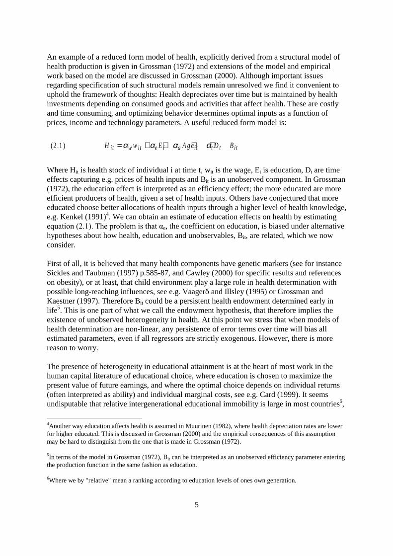
An example of a reduced form model of health, explicitly derived from a structural model ofhealth production is given in Grossman (1972) and extensions of the model and empiricalwork based on the model are discussed in Grossman (2000). Although important issuesregarding specification of such structural models remain unresolved we find it convenient touphold the framework of thoughts: Health depreciates over time but is maintained by healthinvestments depending on consumed goods and activities that affect health. These are costlyand time consuming, and optimizing behavior determines optimal inputs as a function ofprices, income and technology parameters. A useful reduced form model is:

(2 .1 ) H w E A g e D Bit w it e i a it t t i t= + + + +α α α α

Where Hit is health stock of individual i at time t, wit is the wage, Ei is education, Dt are timeeffects capturing e.g. prices of health inputs and Bit is an unobserved component. In Grossman(1972), the education effect is interpreted as an efficiency effect; the more educated are moreefficient producers of health, given a set of health inputs. Others have conjectured that moreeducated choose better allocations of health inputs through a higher level of health knowledge,e.g. Kenkel (1991)4. We can obtain an estimate of education effects on health by estimatingHTXDWLRQ��������7KH�SUREOHP�LV�WKDW�.e, the coefficient on education, is biased under alternativehypotheses about how health, education and unobservables, Bit, are related, which we nowconsider.

First of all, it is believed that many health components have genetic markers (see for instanceSickles and Taubman (1997) p.585-87, and Cawley (2000) for specific results and referenceson obesity), or at least, that child environment play a large role in health determination withpossible long-reaching influences, see e.g. Vaagerö and Illsley (1995) or Grossman andKaestner (1997). Therefore Bit could be a persistent health endowment determined early inlife5. This is one part of what we call the endowment hypothesis, that therefore implies theexistence of unobserved heterogeneity in health. At this point we stress that when models ofhealth determination are non-linear, any persistence of error terms over time will bias allestimated parameters, even if all regressors are strictly exogenous. However, there is morereason to worry.

The presence of heterogeneity in educational attainment is at the heart of most work in thehuman capital literature of educational choice, where education is chosen to maximize thepresent value of future earnings, and where the optimal choice depends on individual returns(often interpreted as ability) and individual marginal costs, see e.g. Card (1999). It seemsundisputable that relative intergenerational educational immobility is large in most countries6,

4Another way education affects health is assumed in Muurinen (1982), where health depreciation rates are lowerfor higher educated. This is discussed in Grossman (2000) and the empirical consequences of this assumptionmay be hard to distinguish from the one that is made in Grossman (1972).

5In terms of the model in Grossman (1972), Bit can be interpreted as an unobserved efficiency parameter enteringthe production function in the same fashion as education.

6Where we by "relative" mean a ranking according to education levels of ones own generation.

6

see Mulligan (1999), and that performance in school is highly related to parents socioecono-mic status, see Heinesen (1999) and Hansen (1999) for Danish results. It therefore makesgood sense to model educational attainment as a function of individual ability and familycharacteristics. When individual ability is positively correlated with health endowments,estimated education effects are upward biased in a linear model, when education is treated asexogenous. This is the endowment hypothesis7.An alternative interpretation of education coefficients was given by Fuchs (1982). Fuchssuggested that differences in time preferences may explain the correlation between educationand health; those paying more attention to future welfare are more likely to engage inactivities with current costs and future benefits, such as education and health investments8.We stress that in order for this to be the explanation, either must health and education affectutility directly, or income must yield utility. If they are wanted only for investment purposes,as is the case in Grossmans pure investment model and in most human capital models ofeducation, time preferences play no part in optimal solutions9. However, a priori it cannot beruled out that unobserved components, Bit, depends on time preferences. If they do, andHGXFDWLRQ�GRHV�DV�ZHOO��.e is again upward biased. This is the time preference hypothesis.

For a comprehensive review of empirical findings within economics, see Grossman andKaestner (1997). In the current context, we stress that in order to be able to distinguishdifferent explanations of why education and health are related, different identificationschemes are needed. We briefly look at some of the methods that have been used.

The by far most common technique is regression analysis, where identification hinges uponuse of adequate controls. One of the most extensive analysis of this kind in this literature, isGrossman (1973). Grossman corrects for "omitted" variables and reverse causality betweeneducation and health by including four different testscore-indices, mother and fatherseducation and health in high school respectively. He finds large and significant direct effectsof both education on SRH and mortality. The drawback of this approach is that it does notallow for effects of unobservables. It is likely that for instance test-scores are only crudeproxies of what we intend to measure, and in some cases this may exacerbate the bias thatexist when the proxy is not included, see e.g. Rosenzweig and Wolpin (1994).

A second approach that circumvents the problems of the first, is to instrument education.Again, different hypotheses require different instruments. If the worry is reverse causality, onemight instrument education with childhood health. If one is worried because of the endow-

7A slightly different story of inverse causality is given in Grossman (1973). There, Bit is an initial (thus timeinvariant) health depreciation value, which affects both child and adult health. When more healthy childrenobtains more education, education becomes indirectly related to Bit� DQG .e will be upward biased. Grossman(1973) later notes that Bit may be related to schooling, essentially because it depends on family characteristics,bringing us back to a common factor explanation. Our approach is more general in distinguishing between twoXQREVHUYHG FRPSRQHQWV� DIIHFWLQJ KHDOWK DQG VFKRROLQJ UHVSHFWLYHO\� 7KH ELDV RI .e is not determined a priori,but depends on the sign of the correlation between "health endowment" and "ability".

8Fuchs also mentions the possibility that schooling has an effect on time preferences, but in his empiricalinvestigations he cannot distinguish between the direction of causality between schooling and time preferences.The latter causality-path has been considered recently at more length by Becker and Mulligan (1997).

9This argument is valid with perfect borrowing markets.

7

ment and the time preference rate hypothesis, one need instruments that are orthogonal tohealth endowments or time preference rates. As discussed by Grossman (2000), the study byBerger and Leigh (1989) is interesting in this respect, because they use per capita income andper capita expenditures on education in the state of birth as instruments for education, whichseems more plausible candidates than e.g. family characteristics and childhood health. Bergerand Leigh find that correcting for endogeneity, education effects are reduced slightly butremains significant. Since they do not discuss or test the validity of their instruments, wemention that in their first stage regression, state per capita expenditure on education has nosignificant effect on education. They apply the method of Garen (1984), which gives directestimates of the effect of unobservables on health. Under the endowment and time preferencehypothesis, unobservables have positive effects on health. In their application, the effects ofunobservables on health are insignificant. Grossman and Kaestner (1997) mention otherstudies investigating the time preference hypothesis, looking at health behavior notably bysmoking, and does therefore not deal with the education gradient in health per se. They doconclude that the existing, sparse evidence does not favor the time preference hypothesis.

Another identification scheme is the use of within family correlations. An example of anapplication of this method is Behrman and Wolfe (1989). They use education of the respon-dents sister as control for endowments and, as suggested by Chamberlain (1980), get anestimate of the true education effect as the difference between coefficients on own educationand sisters education. Behrman and Wolfe also apply the related method of household fixedeffect estimates. These identification strategies are valid when differences in school levelsbetween sisters are unrelated to unobserved determinants of health. Compared to the casewhen no account of unobserved factors is taken, the first method yields smaller educationeffects in the study by Behrman and Wolfe, but they remain of substantial size and aresignificant. The household fixed effect estimator produces larger education effects, as well aslarger imprecision, leaving education significant only at a 10 percent level.

We finally note that none of these studies allow for unobserved individual heterogeneity inhealth over time. As both the endowment and the time preference rate hypotheses imply thathealth is affected by unobserved (possibly) time-invariant factors, this is worth considering. Ifunobserved heterogeneity is an issue, and not taken into account, all non-linear models andmodels which condition on past health (linear as well as non-linear), as in Berger and Leigh(1989) and Grossman (1973), produce inconsistent parameter estimates.

As it stands, although none of these studies suggest that taking care of endogeneity alters theeffect of education by much, no firm conclusion can be reached from the sparse evidence.Furthermore, only one study uses instruments most likely to be robust to heterogeneity in timepreferences and, to our knowledge, none allow for individual specific heterogeneity over time.

3 Empirical Model

Our empirical model is a reduced form model of health and educational determination.Although we will use other health measures in the empirical analysis, in this section wespecify the empirical model using SRH as dependent variable. Education is measured in yearsof education. We model health and education with an ordered discrete response and a linearregression specification respectively:

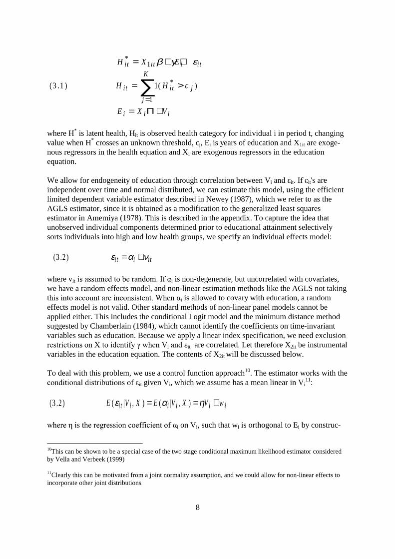
8

(3 .1 )

H X E

H H c

E X V

it it i it

it it j

j

K

i i i

*

*( )

= + +

= >

= +=

∑1

1

1

β γ ε

Π

where H* is latent health, Hit is observed health category for individual i in period t, changingvalue when H* crosses an unknown threshold, cj, Ei is years of education and X1it are exoge-nous regressors in the health equation and Xi are exogenous regressors in the educationequation.

We allow for endogeneity of education through correlation between Vi�DQG�0it��,I�0it's areindependent over time and normal distributed, we can estimate this model, using the efficientlimited dependent variable estimator described in Newey (1987), which we refer to as theAGLS estimator, since it is obtained as a modification to the generalized least squaresestimator in Amemiya (1978). This is described in the appendix. To capture the idea thatunobserved individual components determined prior to educational attainment selectivelysorts individuals into high and low health groups, we specify an individual effects model:

(3 .2 ) ε α νit i it= +

where vit�LV�DVVXPHG�WR�EH�UDQGRP��,I�.i is non-degenerate, but uncorrelated with covariates,we have a random effects model, and non-linear estimation methods like the AGLS not takingWKLV�LQWR�DFFRXQW�DUH�LQFRQVLVWHQW��:KHQ�.i is allowed to covary with education, a randomeffects model is not valid. Other standard methods of non-linear panel models cannot beapplied either. This includes the conditional Logit model and the minimum distance methodsuggested by Chamberlain (1984), which cannot identify the coefficients on time-invariantvariables such as education. Because we apply a linear index specification, we need exclusionUHVWULFWLRQV�RQ�;�WR�LGHQWLI\���ZKHQ�9i�DQG�0it are correlated. Let therefore X2it be instrumentalvariables in the education equation. The contents of X2it will be discussed below.

To deal with this problem, we use a control function approach10. The estimator works with theFRQGLWLRQDO�GLVWULEXWLRQV�RI�0it given Vi, which we assume has a mean linear in Vi

11:

(3 .2 ) E V X E V X V wit i i i i i( | , ) ( | , )ε α η= = +

ZKHUH���LV�WKH�UHJUHVVLRQ�FRHIILFLHQW�RI�.i on Vi, such that wi is orthogonal to Ei by construc-

10This can be shown to be a special case of the two stage conditional maximum likelihood estimator consideredby Vella and Verbeek (1999)

11Clearly this can be motivated from a joint normality assumption, and we could allow for non-linear effects toincorporate other joint distributions

9

tion. Substituting this into the model we get:

(3 .2 ) H X E V wit it i i i i t* = + + + +1 β γ η ν

VXFK�WKDW���FDQ�EH�HVWLPDWHG�FRQVLVWHQWO\�E\�UDQGRP�HIIHFWV��ZKHQ�9i is replaced by aconsistent estimate. We call this estimator the random effects two stage conditional maximumlikelihood estimator, abbreviated 2SMLR. Without the random effects, this is the two stageconditional maximum likelihood estimator (2SCML) considered for the Probit model byRivers and Vuong (1988). Note that under the time preference hypothesis, and if educationability is positively correlated health endowment also under the endowment hypothesis, weH[SHFW���WR�EH�RI�WKH�VDPH�VLJQ�DV���

We accentuate three attractive properties of this model. First, it provides an easy accessibletest for exogeneity of E, namely the t�WHVW�WKDW���LV�]HUR��VHH�5LYHUV�DQG�9XRQJ���������6HFRQG�

testing exclusion restrictions that identify the education coefficient, is easily done in the spiritof tests suggested by Hausman (1978) in a linear model, see e.g. Bollen et al. (1995). Thevalidity of excluding variable X2k can be tested with a t-test that the coefficient correspondingto X2k is zero in the second stage estimation, where X2k is included and the residual Vi isestimated using the other excluded X2 variables. Finally, the specification allows the use ofinstrumental variables generated from X1it as suggested by Hausman and Taylor (1981). Wenote that corrections of standard errors for the first-stage regression are needed for results tobe asymptotically correct, but we have not done that. It therefore might be worth mentioningthat Bollen et al. (1995) mention findings from Monte Carlo investigations, showing no gainin correcting for first-stage estimates for the similar cross-sectional estimator considered byRivers and Vuong (1988).

4 School Reform as Instrumental Variable

In the last section we mentioned that "mechanical" Hausman Taylor instruments can beapplied in the panel model we suggested. These instruments rely on assumptions on thecovariance structure between error terms and regressors, as well as exclusion restrictions ofindividual means over time of exogenous regressors in the health equation. In this section wediscuss the use of other instrumental variables, using information on two school reforms thattook place in Denmark in 1958 and 1975. We use information from yearbooks from theDanish Parliament (Folketingets Årbog, 1903-4, 1957-58 and 1974-75) and Bryld et al.(1990).

In 1904 the middle school (Danish: mellemskolen), classes from grade 6 to 9, was introducedaimed at preparing pupils for gymnasium. Pupils had to pass a test after 5th grade, and thosewho did not pass would continue education for two more years only. The major changeinitiated by the 1958 reform, was that the partition into preschool and middleschool wasabolished. From this year everybody received the same first 7 years of schooling, and formaltests to continue into grades 8-10, preparing for gymnasium, were replaced by teachersrecommendations. In addition, the village school (Danish: landsbyskole) gained the same rightas the city schools (Danish: Købstadsskole), to form classes for grade 8-10, which increasedthe proximity of schools necessary for further education at the countryside. The reform in1975 raised the minimum school-leaving-age, increasing the compulsory years of education

10

from 7 to 9 years. The extent to which this had an impact on mean education is however verydubious, since most children continued into grade 9 voluntarily already. Moreover, manyfactors contributed to the increasing demand for further education in the post-war decades,many of which long before the reforms. For a viewpoint that the 1958-reform was animportant contributor to this development see e.g. Hansen (1982).

We generate two dummy instrumental variables from the 1958 and the 1975 reforms, one forindividuals aged below 34 in 1995 and one for individuals aged between 33 and 51 in 1995.Individuals in the first group were less than 14, i.e. in 7th grade or below, in 1975 and weretherefore affected by the 1975 reform. Individuals in the second group were 14 or above in1975 and less than 14 in 1958, i.e. they were affected by the 1958 reform, but not by the 1975reform. The comparison group is those not affected by any of the reforms.

When are the dummies for whether or not individuals were affected by a school reform validinstruments? The identification scheme used, is known as a regression discontinuity design12.The literature distinguishes between a "sharp" and a "fuzzy" regression discontinuity design,see e.g. Hahn et al. (2001). In the former, the instrumented variable as a function of theinstrument has mechanically determined discontinuity points, in the latter the conditionalprobability distribution of the instrumented variable given the instrument has discontinuitypoints. In an ideal world these breaks generate natural experiments, creating exogenouschanges in endogenous variables. In our case, the 1975 school reform ensures that the lengthof education is at least 9 years, such that those who wanted to stop after seven years are forcedinto education, thus resembles a sharp design. If anything, the 1958 reform is a fuzzy design,in that it lowers barriers for further educational beyond grade 7. Below we check the fuzzydesign by calculating the share with given educational attainment at given ages in our sample.

There are other concerns related to the use of discontinuity designs. First, as all instruments, itmust be uncorrelated with the unobservables determining the main outcome variable.Therefore we need to take account of upward drifts over time in health, which are automati-cally positively correlated with the increases in education implied by the instruments. To dothis we have to assume that other events, driving the upward drifts, can be captured bypreferably linear cohort effects, to diminish the multicollinearity between school reformdummies and the drifts.

There are several other points that must be considered when using IV estimation. It has beenshown that when instruments and endogenous explanatory variables are only weakly correla-ted, inconsistency of IV-estimates relative to OLS may blow up, see e.g. Bound et al. (1995).The relative inconsistency is inversely proportional to the partial R-squared of the instrumentsin the first stage estimation. A second problem is that IV estimates are biased towards OLS infinite samples, a bias which can be substantial even in very large samples. The bias has beenshown to be inversely proportional to the F-statistic on instruments in the first stage. It istherefore informative to report the partial F-statistic and R-squared on the instruments fromthe first stage estimation. Finally, a linear IV-estimator identifies a weighted average of the

12A well-known example in economics is Maimonides' rule, applied as an instrument for class size effect ontest-scores, see e.g. Angrist and Krueger (1999). An example of use of school reforms is given in Harmon andWalker (1995), estimating the returns to schooling on wages.

11

effects in the sub-populations affected by the school-reform, see e.g. Card (1999) p.1821. Inour specific case, if education effects are heterogeneous, the estimated effect will be aweighted mean of effects for those individuals affected by the reform (a local averagetreatment, or LATE, effect). These are most likely to be individuals from families from thecountryside and individuals who were least likely to have been sorted in to the middleschool.Because these individuals are likely to have low health, we argue that even withheterogeneous education effects, the estimates are of considerable interest.

5 Data

We use a two-period data set of Danish workers interviewed in 1990 and 1995 (The DanishNational Work Environment Cohort Study (WECS)). Since we will use the panel structure ofthe data, we only use observations with valid data in both 1990 and 1995. The data setincludes self-reported health, graded as poor, fair, good, very good and excellent, which willbe our main health outcome, as well as socio-economic information on education, occupation,work type-and time, and a large array of work environment variables. Because the educationvariables differ in the two surveys, we choose to use the 1995 question, combined withinformation on primary schooling if no education is undertaken. A more detailed descriptionof the data and our specific sample, education, occupation, industry and regional variables, aswell as the construction of the hourly wage, is found in the appendix. We end up with 2023men and 1732 women who are observed in both 1990 and 1995. As our sample does not differmuch with respect to age, education and occupational distribution, from the unbalancedsample, see Borg and Burr (1997), we preserve a reasonable representative national sample ofindividual workers employed within the last two months who have finished their education.

Finally a word on the SRH variable. SRH it is generally believed to be a useful summarymeasure of health, since it allows to measure health at the individual level, and is believed tocapture important intervening mechanisms leading to increased risk of functional disabilityand mortality, see e.g. Idler (1994). Furthermore, the common inclusion of SRH in health andsocioeconomic surveys makes it easy to compare results with other findings. However, a largedebate on possible measurement error in SRH exist, see e.g. Butler et al. (1987) or Benítez-Silva et al. (1999), but since we instrument education, measurement error in SRH that isrelated to education is likely to be of minor importance13.

For robustness, we also apply the following alternative measures of health: self-reportedweight and height to form the body mass index14, self-reports of whether never been smoking,years of smoking and whether a doctor has informed the interviewed that he or she has highblood pressure (HBP).

13Given that our instruments are unrelated to the measurement error.

14Weight in kg, divided by height in meters squared.

6 Results

12

6.1 Descriptive Statistics

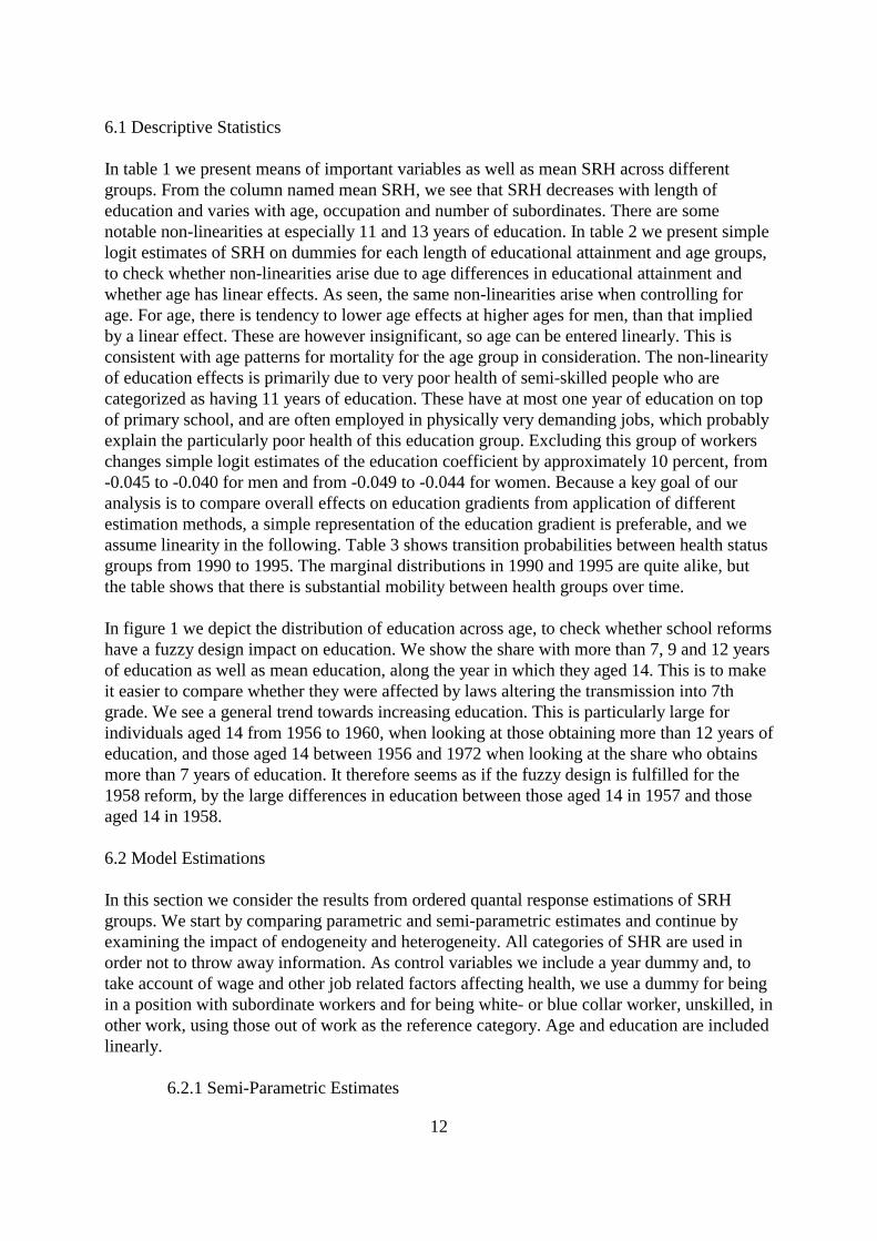
In table 1 we present means of important variables as well as mean SRH across differentgroups. From the column named mean SRH, we see that SRH decreases with length ofeducation and varies with age, occupation and number of subordinates. There are somenotable non-linearities at especially 11 and 13 years of education. In table 2 we present simplelogit estimates of SRH on dummies for each length of educational attainment and age groups,to check whether non-linearities arise due to age differences in educational attainment andwhether age has linear effects. As seen, the same non-linearities arise when controlling forage. For age, there is tendency to lower age effects at higher ages for men, than that impliedby a linear effect. These are however insignificant, so age can be entered linearly. This isconsistent with age patterns for mortality for the age group in consideration. The non-linearityof education effects is primarily due to very poor health of semi-skilled people who arecategorized as having 11 years of education. These have at most one year of education on topof primary school, and are often employed in physically very demanding jobs, which probablyexplain the particularly poor health of this education group. Excluding this group of workerschanges simple logit estimates of the education coefficient by approximately 10 percent, from-0.045 to -0.040 for men and from -0.049 to -0.044 for women. Because a key goal of ouranalysis is to compare overall effects on education gradients from application of differentestimation methods, a simple representation of the education gradient is preferable, and weassume linearity in the following. Table 3 shows transition probabilities between health statusgroups from 1990 to 1995. The marginal distributions in 1990 and 1995 are quite alike, butthe table shows that there is substantial mobility between health groups over time.

In figure 1 we depict the distribution of education across age, to check whether school reformshave a fuzzy design impact on education. We show the share with more than 7, 9 and 12 yearsof education as well as mean education, along the year in which they aged 14. This is to makeit easier to compare whether they were affected by laws altering the transmission into 7thgrade. We see a general trend towards increasing education. This is particularly large forindividuals aged 14 from 1956 to 1960, when looking at those obtaining more than 12 years ofeducation, and those aged 14 between 1956 and 1972 when looking at the share who obtainsmore than 7 years of education. It therefore seems as if the fuzzy design is fulfilled for the1958 reform, by the large differences in education between those aged 14 in 1957 and thoseaged 14 in 1958.

6.2 Model Estimations

In this section we consider the results from ordered quantal response estimations of SRHgroups. We start by comparing parametric and semi-parametric estimates and continue byexamining the impact of endogeneity and heterogeneity. All categories of SHR are used inorder not to throw away information. As control variables we include a year dummy and, totake account of wage and other job related factors affecting health, we use a dummy for beingin a position with subordinate workers and for being white- or blue collar worker, unskilled, inother work, using those out of work as the reference category. Age and education are includedlinearly.

6.2.1 Semi-Parametric Estimates

13

As a starting point, we consider robustness issues assuming all regressors are exogenous.Results from an ordered probit model are presented in column (1) in table 4 for men, and incolumn (4) for women. One alternative estimator for our model, is the semiparametricmonotone rank (MR) estimator suggested by Cavanagh and Sherman (1998). This estimatormakes no distributional assumptions, is very general in functional form and is consistentunder certain types of heteroscedasticity. It is described in the appendix. To compare probitestimates with semiparametric estimates, we have normalized all coefficients setting the agecoefficient to one15. The standard errors of the probit estimates are calculated using the deltamethod16. The MR estimates are presented in column (3) and (6) of table 4. Logits areincluded in columns (2) and (5) for completeness. The semiparametric estimates differ fromthe parametric estimates. A priori the conditions are fulfilled for conducting a Hausmanmisspecification test, since both the MR and MLE estimators are root-n asymptotic normalunder the null, that the conditions for the MLE are fulfilled. In practice, when covariancematrices are estimated, the difference in covariance matrices between the MLE and MR isindefinite17, so the Hausman test cannot be carried out. We note though that MR-educationcoefficients are of the same sign as ML-coefficients and they are significant. The MRestimates for the education coefficient is 26 percent higher for men and 10 percent lower forwomen than the logit estimate. The key assumption driving consistency of the MR estimatorLV�WKDW�WKH�PHDQ�RI�WKH�GHSHQGHQGHQW�YDULDEOH�LV�PRQRWRQLF�LQ�WKH�HVWLPDWHG�LQGH[�;���7KLV�LV

required for ordered logit and probit models as well. We check this by non-parametricUHJUHVVLRQ�RI�65+�RQ�WKH�HVWLPDWHG�LQGH[�;���XVLQJ�WKH�05�HVWLPDWHV�RI����VHH�WKH�DSSHQGL[

15The MR estimator is estimated with GAUSSTM, ver. 3.2.4, using a Fortran minimization procedure fromNumerical Recipes (www.nr.com) and is written in GAUSS by Bo E. Honoré. We thank him for making the codeavailable to us, which we of course use on our own responsibility. The variance estimates are obtained using theformulas in Cavanagh and Sherman (1998), and conditional means and densities in these formulas are estimatedby kernel estimation. We use gaussian kernels and Silvermans rule of thumb bandwidth.

162EWDLQHG DV IROORZV� ZKHUH �a LV WKH DJH FRHIILFLHQW DQG � DUH DOO RWKHU FRHIILFLHQWV�

cov ( ) ( ) cov ( , ) ( ),

( ) [/

,/

] [ , ]

ββ

ββ

β β ββ

ββ

∂β β∂β

∂β β∂β β

ββ

a aa

a

a

a a

a a a

= ∇ ∇

∇ = = −

w h ere

12

17It has both positive and negative eigenvalues.

14

for details. The results are shown with 95 percent pointwise confidence bands in figure 2 forwomen and in figure 3 for men. The plots are very smooth and although there are smallregions of nonmonotonicity, they are insignificant. The consistency of the MR estimator issupported by the finding that results are not affected by excluding the fifth of individuals withlow index values, which seems to be the region with largest possibility of non-monotinicities.

6.2.2 Logit Estimations

In this section we present results from estimations based on parametric estimators includingthe 2SMLR estimator discussed earlier. We have seen in the last section that parametricestimations are fairly robust to functional and ditributional form. Since it does not seem tomatter whether to use a probit or a logit specification, we choose the logit.

Table 5a and 5b contain the results applying different versions of the ordered logit model,namely the simple ordered logit, the ordered logit with random effects, the AGLS and the2SCML, both with no random effects but endogenous education, and finally the 2SMLRestimator. Recall that our health measure is 1 for excellent health and 5 for poor health,implying that a negative coefficient shows that the corresponding variable varies positivelywith better health.

Starting with the results for men, in table 5a column (1), the simple ordered logit is presented.Both education and occupation variables are significant, education with a coefficient of-0.041, such that more educated have better health, white collar workers are more healthy thanblue collar and unskilled workers, but of similar health as those in other types of work. It isalso observed that having any subordinate workers indicates better health also in this multi-variate framework. In column (2) we take account of unobserved heterogeneity, allowing forindividual random effects being correlated over time for each individual. We use a discretefactor approximation to estimate the distribution of individual effects, see for instance Mrozand Guilkey (1995), i.e. we do not make any distributional assumptions18. The location andmasspoints of these points are estimated freely. For the 2SMLR estimator presented in column(6), a discrete distribution with three points of support is found to fit the data better than twoand equally good as four. We use three points of support in other random effects estimationsas well. We see from column (2), that when random effects are included, the educationcoefficient increases in magnitude and remains significant.

The presence of random effects is tested, comparing estimations in (1) and (2) by means of alikelihood ratio test. Minus two times the log likelihood ratio is presented in the first rowbelow parameter estimates. This is chi-squared distributed with five degrees of freedom, thenumber of parameters in the random effects distribution19. As the critical value in thisdistribution at a five percent level is 11.07, and the observed test statistic is 219.3, we rejectthe null of no heterogeneity.

18Estimations are conducted using StataTM ver. 6.0, using the program GLLAMM ver. 6, see Rabe-Hesketh et al.(2001).

19Three mass points and two probabilities that vary freely.

15

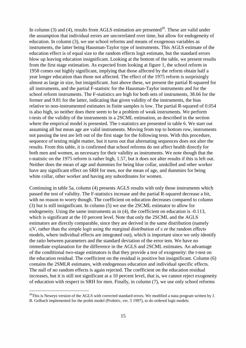
In column (3) and (4), results from AGLS estimation are presented20. These are valid underthe assumption that individual errors are uncorrelated over time, but allow for endogeneity ofeducation. In column (3), we use school reforms and means of exogenous variables asinstruments, the latter being Hausman-Taylor type of instruments. This AGLS estimate of theeducation effect is of equal size to the random effects logit estimate, but the standard errorsblow up leaving education insignificant. Looking at the bottom of the table, we present resultsfrom the first stage estimation. As expected from looking at figure 1, the school reform in1958 comes out highly significant, implying that those affected by the reform obtain half ayear longer education than those not affected. The effect of the 1975 reform is surprisinglyalmost as large in size, but insignificant. Just above these, we present the partial R-squared forall instruments, and the partial F-statistic for the Hausman-Taylor instruments and for theschool reform instruments. The F-statistics are high for both sets of instruments, 38.66 for theformer and 9.81 for the latter, indicating that given validity of the instruments, the biasrelative to non-instrumented estimates in finite samples is low. The partial R-squared of 0.054is also high, so neither does there seem to be a problem of weak instruments. We performt-tests of the validity of the instruments in a 2SCML estimation, as described in the sectionwhere the empirical model is presented. The t-statistics are presented in table 6. We start outassuming all but mean age are valid instruments. Moving from top to bottom row, instrumentsnot passing the test are left out of the first stage for the following tests. With this procedure,sequence of testing might matter, but it turns out that alternating sequences does not alter theresults. From this table, it is confirmed that school reforms do not affect health directly forboth men and women, as necessary for their validity as instruments. We note though that thet-statistic on the 1975 reform is rather high, 1.57, but it does not alter results if this is left out.Neither does the mean of age and dummies for being blue collar, unskilled and other workerhave any significant effect on SRH for men, nor the mean of age, and dummies for beingwhite collar, other worker and having any subordinates for women.

Continuing in table 5a, column (4) presents AGLS results with only those instruments whichpassed the test of validity. The F-statistics increase and the partial R-squared decrease a bit,with no reason to worry though. The coefficient on education decreases compared to column(3) but is still insignificant. In column (5) we use the 2SCML estimator to allow forendogeneity. Using the same instruments as in (4), the coefficient on education is -0.113,which is significant at the 10 percent level. Note that only the 2SCML and the AGLSestimators are directly comparable, since they are derived in the same distribution (namely0_9��UDWKHU�WKDQ�WKH�VLPSOH�ORJLW�XVLQJ�WKH�PDUJLQDO�GLVWULEXWLRQ�RI�0�RU�WKH�UDQGRP�HIIHFWV

models, where individual effects are integrated out), which is important since we only identifythe ratio between parameters and the standard deviation of the error tem. We have noimmediate explanation for the difference in the AGLS and 2SCML estimates. An advantageof the conditional two-stage estimators is that they provide a test of exogeneity: the t-test onthe education residual. The coefficient on the residual is positive but insignificant. Column (6)contains the 2SMLR estimates, with endogenous education and individual specific effects.The null of no random effects is again rejected. The coefficient on the education residualincreases, but it is still not significant at a 10 percent level, that is, we cannot reject exogeneityof education with respect to SRH for men. Finally, in column (7), we use only school reforms

20This is Neweys version of the AGLS with corrected standard errors. We modified a stata program written by J.B. Gelbach implemented for the probit model (Probitiv, ver. 5 1997), to do ordered logit models.

16

as instruments in the first stage estimation. As seen from the bottom of the table, while theF-statistic hardly changes, this dramatically reduces the partial R-squared, indicating aproblem of weak instruments. We note that a partial R-squared of 0.005 is about 50 timeshigher than the famous quarter of birth instruments used by Card and Krueger, see Bound etal. (1995). However, this does not alter that most of the identification in the previousestimations came from the assumptions justifying use of Hausman-Taylor instruments. Botheducation and residuals are now insignificant.

Moving forward to table 5b, we look at results for women. The estimators with no randomeffects are again rejected, where a better fit is obtained using three rather than two points ofsupport for the random effect, and no gain is obtained using four points. From the first stageestimations, we see that the F-statistic on school reform instruments is a bit lower than wasthe case for men, 3.78, although still being above the 95 percent quantile. Overall, with theexception of column (7), there is no evidence of substantial finite sample bias nor of weakinstruments. The AGLS estimate in column (3) with all means of exogenous variables asinstruments, is now very large in magnitude and significant. When excluding instrumentswhich did not pass the validation test, see table 6 again, the AGLS estimate of the educationcoefficient is however similar to the random effects estimate, but insignificant. In the firststage estimation, the effect of the 1975 school reform on education is small and insignificant,and the 1958 reform increases length of education now only by a quarter of a year, which issignificant at a 10 percent level. The 2SMCL estimate of the education coefficient is -0.188and significant. The coefficient on the education residual is positive, but now, as opposed tothe case for men, highly significant. Moving to column (6), taking account of heterogeneity,the education residual and the education effect increases further in magnitude, both still beingsignificant. In column (7) we only use school reforms as instruments, and although theresidual and education effects increase further in magnitude, they become insignificant.

6.2.3 Alternative Health Measures

Because health has many dimensions, more robust results are obtained by using several healthmeasures. We therefore repeat estimations from the last section using the BMI, HBP andsmoking variables mentioned earlier. One might argue that these variables reflects "riskfactors" that are more closely related to health inputs rather than health outcomes, and for thisreason we also estimate a model using SRH as outcome, including these health three othervariables as explanatory variables. This can be interpreted as an estimate of a productionfunction of health, and can be used to assess the size of the education gradient given healhinputs, thus to distinguish between productive and allocative efficiency. We do not at thisstage account for endogeneity of health inputs21. When the dependent variable is an input tohealth production, education effects reflect allocative efficiency, but may be biased for theexact same reasons as they are in estimations with health outcomes.

In table 7 means and standard deviations of these other health measure are presented, as wellas their correlation with education and SRH. We have included indicators of being fat andobese, defined as BMI above 25 and 30 respectively, as these are commonly applied healthmeasures in the medical literature. Although there is no general agreement on optimal BMI for

21See Gilleskie and Harrison (1998) for a thorough investigation of this type.

17

good health, obesity in particular is seen as a large health threat, which besides implyingpossible physical restrictions, stigmas and psychological pains, increases the risk of e.g.cardiovascular diseases and diabetes, see e.g. the report edited by Thomas (1995). From table7, we see that men have larger BMI; the mean of BMI is higher and the shares of fat and obesemen are higher for men than for women. In our sample, 44 percent of the men, whereas only19 percent of the women, are classified as being fat. Moreover, men smoke more and aroundseven percent of both men and women have been diagnosed having high blood pressure. Asseen in the third column of the table, all, except high blood pressure, these alternative healthmeasures have quite high correlations with education. The fourth column shows that all thealternative health measures are correlated with SRH, including high blood pressure.

Results for BMI and the indicator of never been smoking (NS) are presented in table 8. Thesame estimations were conducted for HBP, but are left out, since only age showed upsignificant and education effects were small in size as well as insignificant. Three estimationsare presented for each health measure. One with exogenous regressors and no individualeffects, one with random effects and one with random effects and endogenous education (the2SMLR estimator). Because most occupation dummies were insignificant, we conducted2SMLR estimations with only the one occupation group, that deviated most from the others.Tests of validity of instruments are presented in table 9. We use linear regression model forBMI and a logit model for NS. The null hypothesis of no random effects is rejected in allmodels. Education is significant at a five percent level in all estimations, except for the2SMLR estimation of womens BMI. However, the null hypothesis of exogeneity of educationis rejected for both BMI and NS for men but cannot be rejected for women, that is, theopposite to that found using SRH. Moreover, while education has the expected sign; moreeducated have less BMI and a higher share have never smoked, education residuals work inthe opposite direction, as found for SRH.

Table 10 contains estimations of a health production function using simple ordered logit.From these results we note that for both men and women, the education coefficients remainsignificant, although reduced by 31 percent for men, and 16 percent for women whencompared to the model without health inputs. All three risk factors have the expected sign,and have larger effects on men than women on SRH. Although the interpretation of thisestimation as a production function estimate may be dubious, the results show that SRH ishighly related to other common measures of (threats to) health conditions. Moreover, it alsoshows that SRH has a social gradient on top of these standard risk factors, and as suchconfirms our initial hypothesis that something else than healthy behavior explains thegradient. However, the result may arise because of reporting error in SRH, when this error isrelated to social status. A suggestive test for how this additional dimension of SRH relates tocognitive aspects influencing feelings of well being, was conducted by Grossman (1973). Heincluded an indicator of job satisfaction, on the grounds that if (less) better educated onaverage are more (dis-) satisfied with their lives, they may tend to (under-) over report SRH.Even when life satisfaction is not related to health, we would therefore observe a educationgradient in SRH. If life satisfaction is captured by job satisfaction, education gradients shouldvanish when this is included as control. As seen in column (2) and (4) job satisfaction alsocomes out highly significant in magnitude and in statistical terms, but more importantly, thesocial gradient in SRH does not diminish, supporting hypothesis that SRH captures conditionsimportant to health on top of risk factors.

18

7 Discussion and Conclusion

It has been documented extensively that educational differences in health exist. Far lessinvestigations have considered whether the observed relationship has a causal componentfrom e.g. education to health. Can the education related differences in health we observe beinterpreted as partly reflecting a return to education? The answer to this question is oftremendous importance to our understanding of how health is determined, and how it may beaffected.

We have tried to investigate to what extent heterogeneity in health and endogeneity ofeducation explained the education gradient in health, using SRH, BMI and indicators for highblood pressure (HBP) and never been smoking (NS). With one exception the results of ouranalysis do not invalidate hypotheses about direct educational effects on SRH, BMI and NSvariables. Although e.g. Berger and Leigh (1989) did find an educational gradient in bloodpressure, we did not. This might because our HBP variable is not very precise, indicatingwhether the individual has ever been diagnosed as having blood pressure. For the three othermeasures education gradients are present, even when accounting for occupational differencesusing the semiparametric MR estimator, which is consistent under far more general functionalforms than standard parametric models. Moreover, with our particular data set and assumingonly exogenous regressors, simple ordered probit and logit estimators of SRH did pretty wellcompared to this estimator. For simplicity we have focused on the logit parameters rather thanmarginal effects. To illustrate the magnitude of the estimated differences, we have calculatedodds ratios of having excellent health using predicted probabilities at mean of other regressorsthan education. For the simple logit model (column (1) in table 5), comparing with those withonly seven years of education, odds ratios of having excellent health is 1.5 and 2.1 for menand 1.55 and 2.25 for women with thirteen and eighteen years of education respectively. Wealso showed that we could not reject the presence of heterogeneity in health, accounted for byrandom individual effects in parametric models, in all our models for both men and women.

The evidence on endogeneity of education is more mixed, and we discuss this at some lengthin this section. Using SRH we reject that education is exogenous for women, but not for men.However, using BMI and NS we found the opposite. Education effects are hardly altered whentaking account of endogeneity with the AGLS estimator, which however, in spite ofasymptotic efficiency had a very low small sample precision in our application. When usingthe 2SCML or 2SMLR estimators, education effects are significant. We tried to captureexogenous variation in education by means of school reforms as instruments for education.We showed that education did jump to another level in the years following the 1958 reform,implying that those men affected by this reform have almost half a year longer education,while women have a third of a year more, than those not affected by the reform, on top of acommon age trend. Moreover, no clear indication on small sample bias is found, althoughsome indication of weak instruments when using only school reforms was present. Taking the2SMLR estimators at face value, for all health measures where education is endogenous, thecoefficient on education residuals have the opposite sign as that on education. Since thecoefficient on the education residual estimates the regression coefficient of unobserved healthcomponents on unobserved education components, the latter result is inconsistent with anhypothesis that education and health are determined by a common unobserved factor like timepreferences. Moreover, the result would indicate that individuals with higher school ability

19

have lower health endowments, or put in another way, that if high school ability individualsdid not receive high education, they would have had worse health. Indeed, although logit and2SMLR estimates are not directly comparable (because they are derived in a marginal and aconditional distribution) there is a tendency for education effects to magnify when accountingfor endogeneity. In fact, using the 2SCML estimates to calculate odds ratios of excellenthealth, the large simple logit differences increase to 3.5 and 9.9 for men and 7.4 and 38.8 forwomen. In terms of a local average treatment effects interpretation, see section 4, it means thatthose high ability children who received more education due to the school reforms, gainedsubstantially in health from the increased education. This interpretation, although worthnoting, is perhaps too strong. First of all, we only follow individuals over five years, which isperhaps too low a time span, if the aim is to capture individual persistence in health possiblydating back to childhood. Second, the large coefficients on education and education residualsmay stem from a multicollinearity problem, especially when few instruments are used. Moreknowledge on the behavior of the 2SCML estimator in small samples is needed to judge aboutthis. For comparison we estimate simple linear probability models for SRH. An advantage oflinear probability models is that individual effects can be differenced out, 2SLS techniquescan be used, which more applied researchers are familiar with and finally, the conditionalmaximum likelihood estimator, which we call the control function estimator in the linearversion, is algebraically identical to 2SLS. Results are presented in table 11. Comparing theOLS and the 2SLS estimates, we see that instrumenting education, education effects increases,in particular for women. For women, education effects are in fact significant at a ten percentlevel when only using school reforms as instruments, although this is far from the case formen. Adding fixed effects to the 2SLS estimation, using a Hausman-Taylor estimator,increases education effects further. This is also the case for the control function estimates inthe last column. These results support the findings from the 2SCML and 2SCMLR estimates,that education effects are substantial and larger when accounting for endogeneity of educationand heterogeneity in health.

Another issue is that because the instruments we generate from the school reforms, essentiallycompare individuals of very different age, numerous sources may cause health to differbetween the comparison groups, even when accounting for trends in age. Therefore weconduct 2SMLR estimations for SRH in the sample of individuals aged 47 to 54 in 1995, thatis, for individuals entering 7'th grade in one of the four years just before the 1958 reform andindividuals who entered in the four years just after. For this group of individuals there are 854men and 890 women. This does in fact change the results, since the effect of the educationresidual become significant at a 10 percent level for men, whereas it becomes insignificant forwomen. For both however, the education coefficient is substantial and significant, for menthough at a ten percent level.

We make a further note on the intepretation of education effects. Since we were not able tocontrol for wages or income in the panel analysis, education effects may reflect wage orincome effects. We argue that this is likely to be part of, but not the entire story. First of all,we did control for occupational groups and having subordinate workers, which to some extentcapture wage differences. Second, existing evidence suggest that whereas education effectsare quite strong at most education levels, income effects are not as strongly graded, but areconfined to a higher extent among low income levels, showing evidence of education effectsseparate of wage or income effects. We confirmed this in another study, using the same data,Arendt (2001b), where we used wage information in the data set used here, for the 1995

20

period only, and on US data in Arendt (2001a).

Finally we showed that education is related to SRH when controlling for the three other healthmeasures, which can be interpreted as inputs in health production. As such it confirmsGrossman's efficiency hypothesis. It also supports hypotheses of other non-behavioralhypothesis of social gradients in health, e.g. relying on psychosocial factors as described forinstance by Adler et al. (1994).

Although, as summarized above, there are a number of issues regarding both methods anddata that can be improved, we have added to the existing literature, applying identificationtechniques not previously used in this literature and showed that an overall conclusion, whichis supportive of a direct effect, through both allocation (health behavior) and efficiency, ofeducation, is fairly robust.

21

8 Appendix

8.1 Definition of Variables and Sample Selection

The WECS was collected by the Danish National Institute of Occupational Health (AMI) andthe National Institute of Social Research (SFI) as a representative survey of Danish citizensaged 18-59 in 1990 with a follow-up survey in 1995, added with persons to make it represen-tative as well. The sampling method and representativeness of the data is described in detail inNord-Larsen et al. (1992) and Borg and Burr (1997). The total sample of individuals selectedfor interviews in 1990 and 1995 consists of 11084 individuals, each with an individualidentifier. The response rate was 89.7 percent in 1990 and 80.2 percent in 1995.

We create our sample in the following way. We drop 911 observations with missing educationinformation in both 1990 and 1995. Then we drop 702 of the remaining individuals who areunder education in 1990, since we are interested in the effect of completed education. 38 areexcluded because they have missing, no or untold education in 1995, in addition to missing oruntold schooling in 1995 and untold education in 1990. 2946 observations are deleted becauseindividuals were not interviewed in both years. For 10 individuals, their age (defined as yearminus year of birth) is reported as more than 6 or less than 4 years in 1995 from the reportingin 1990, i.e. erroneously, so we delete these. Among the now 6477 remaining observations,we only keep the 3755 with non-missing SHR in both 1990 and 1995, consisting of 2023 menand 1732 women who are observed in both 1990 and 1995. The large numbers of missingobservations are present because this question were only asked to people who were employedwithin the last two months of the interview. Among the 3755, 3673 are in work in 1990 and3675 in 1995.

The education variables differ in 1990 and 1995, because of a finer distinction betweenvocational educations in 1995, and because short advanced degree is not referred to asadvanced (videregaaende) in 1990. We therefore chose to use the 1995 classification in 1990as well to get a consistent time-invariant measure of education. When both educationvariables are missing, we use the schooling variable in 1995. Years of education are definedas follows: 7 years: 7th Grade, 9 years: 9th Grade, 10 years: 10th Grade, 11 years: one yearEFG or semi-skilled (specialarbejdere), 12 years: Gymnasium or Other Short Educ, 13 years:Apprenticeship/EFG, 14 years: Short Advanced, 16 years: Medium Advanced, 18 years: LongAdvanced.

Occupational categories also differ between 1990 and 1995. In 1995 there is only one group ofwhite collar workers (funktionære), but in 1990, there are two (funktionær med mindst et aa rsuddannelse og en underordnet, samt underordnede funktionære), which therefore are collap-sed. Blue collar and unskilled workers (faglærte, ufaglærte) are defined in both years, andused. Finally we define a dummies for people in other types of work (arbejde iøvrigt) and arest category.

In Borg and Burr (1997), it is documented that the sample of interviewed employed persons isrepresentative to reasonable degree with respect to distribution of age, education and occupa-tion. Comparing our sample with the original sample, see Borg and Burr (1997) table 2.5-2.7,people with advanced education and white collar workers are slightly overrepresented,

22

whereas younger and those with only primary school are underrepresented in our sample. Onereason could be that we exclude those under education, who are included in the tables in Borgand Burr (1997) if they have been employed within two months. Overall, we think the sampleis reasonable representative of people who have finished their education and employed withintwo months.

8.2 The AGLS Estimator

1HZH\V�YHUVLRQ�RI�WKH�$*/6�HVWLPDWRU�LV�EDVHG�RQ�WKH�FRQGLWLRQDO�GLVWULEXWLRQ�RI�0�JLYHQ�9

(as opposed to Amemiyas estimator (1978) which was obtained in the marginal distribution of0��LQ��������XVLQJ�WKH�UHGXFHG�IRUP�RI�WKH�+ -equation:

H X X V uit it it i i t* = + + +1 1 2 2α α λ

ZKHUH�� �����DQG�WKH�.V�DUH�UHODWHG�WR�WKH�VWUXFWXUDO�SDUDPHWHUV������DQG���E\�

α β γ α γ1 1 1 2= + =Π Π,

ZKHUH���LV�VSOLW�LQWR��1 DQG��2 according to the variables X1 and X2. From the latter equations,��DQG���FDQ�EH�IRXQG�E\�PLQLPXP�GLVWDQFH��XVLQJ�HVWLPDWHG�.V�DQG��V�

8.3 Cavanagh and Shermans Semiparametric Estimator

The semiparametric estimator suggested by Cavanagh and Sherman (1998) is used as analternative estimator. The estimator is applicable to models of the form:

y D F X= ( ( , ))β ε

ZKHUH�0�LV�D�UDQGRP�HUURU�WHUP��'�LV�D�QRQ�FRQVWDQW�DQG�PRQRWRQH�IXQFWLRQ�DQG�)�LV�D�VWULFWO\

monotonic function. This specification is very general and includes e.g. linear regression,censored regression, transformation, duration and ordered quantal response models, see Han��������&DYDQDJK�DQG�6KHUPDQ�VXJJHVW�WR�HVWLPDWH���E\�WKH�PRQRWRQH�UDQN��05��HVWLPDWRU

defined by:

� arg m ax ( ) ( )β ββ= ∑ M y R Xi ii

where M is an increasing function and R is the rank function, i.e. the number of observationswith index less than or equal to the index of the i'th observation. It is assumed that E(M(y)|X)GHSHQGV�RQO\�RQ�;�WKURXJK�;��DQG�WKDW�LW�LV�LQFUHDVLQJ�LQ�;���&DYDQDJK�DQG�6KHUPDQ�SURYH

that the estimator is root-n consistent when M is deterministic or equal to R. We apply theversion of the estimator with M(y)=y. The estimator is developed for exogenous regressorsand we are therefore relegated to study the biases of functional form misspecificationseparately from that of endogeneity and heterogeneity biases. The semiparametric MR isasymptotic normal and consistent under suitable regularity conditions far more general than

23

those needed for the MLE.

:KHQ�FKHFNLQJ�WKH�DVVXPSWLRQ�WKDW�(�\_;���LV�PRQRWRQLF��ZH�XVH�WKH�ORFDO�OLQHDU�VPRRWKHU�

see below, with a qubic weight function, and a bandwidth, which we weight with densityestimates to get a variable bandwidth. The density is estimated using Silvermans ru-le-of-thumb bandwidth: 0.9*min(stdev(x), interquartile range(x)/1.34). The confidence bandsare calculated, ignoring the bias, using expressions of the asymptotic variance, see below.

8.4 The local linear smoother

The local linear smoother estimate of the conditional mean of y given x is given as pointwiseweighted least square estimations:

E y x a b x

a b y x Kx x

hw

i x x

x x ii

i

i

n

( | )

( , ) a rg m in ( ( )) ( )( , )

= +

= − + −

=∑

, w h ere :

α β α β 2

1

where K is a kernel function (typically a distribution function), h is a bandwidth (a windowthat determines over what range of x's the smoothing is done) and w is a population weight22.If the nearest neighbour method is used instead of a fixed bandwidth, the Lowess estimator byCleveland (1979) is obtained. According to Fan (1992) the estimator is asymptotic normal,with asymptotic variance given by:

Vx

f x nhK u du= ∫σ2

2( )

( )( )

ZKHUH�1 2(x)=V(y|x) is the conditional variance of y given x, f(x) the density of x and n is the

VDPSOH�VL]H��1 2(x) can be estimated by nonparametric regression methods as well. We use the

.HUQHO�HVWLPDWRU�WR�HVWLPDWH�ERWK�1 2(x) and f(x). The kernel regression and density estimators

are given as:

� ( | )( )

� ( ), � ( ) ( )E y x

Kx x

hy

f xf x

n hK

x x

h

ii

i

ni

i

n

=

−

= −

= =∑ ∑

1 1

1

22The local linear smoother estimator has been shown to possess good properties compared to othernon-parametric smoothing methods. Compared to the Nadaraya-Watson kernel estimator, the asymptotic bias issmaller, the asymptotic variance the same, it is not more biased near the boundary points of the support ofregressors and the small sample behavior is better, see Fan (1992).

24

9 References

Acheson, D. 1998. Independent Inquiry into Inequalities in Health Report, The StationaryOffice. (Web: http: //www.official-documents.co.uk/document/doh/ih/contents.htm).

Adler, N., Boyce, T., Chesney, M., Choen, S., Folkman, S., Kahn, R. and Syme, S. (1994).Socioeconomic Status and Health, the Challenge of the Gradient. American Psychologist 49(1):15-24.

Amemiya, T. (1978). The Estimation of a Simultaneous Equation Generalized Probit Model,Econometrica 46 (5), 1193-1205.

Angrist, J. D. and A. B. Krueger (1999). Empirical Strategies in Labor Economics, in:Ashenfelter and Card (Eds.), Handbook of Labor Economics 3A, Elsevier Science,Amsterdam, 1277-1398.

Arendt, J. N. (2001a). Education vs. Income Gradients in Health; Gender and Life CourseSpecific Differences, mimeo, Institute of Economics, University of Copenhagen.

Arendt, J. N. (2001b). Education and Wage Gradients in Self-Reported Health in Denmark,mimeo, Institute of Economics, University of Copenhagen.

Becker, G. and C. Mulligan (1997). The Endogenous Determination of Time Preference.Quarterly Journal of Economics, 112 (3), 729-758.

Behrman, J. and B. Wolfe (1989). Does More education Make Women Better Nourished andHealthier? Journal of Human Resources 24 (1), 644-663.

Berger, M. and J. Leigh (1989). Education, Self-Selection and Health, Journal of HumanResources 24 (1), 433-455

Bollen, K. A., Guilkey, D. K. and T. A. Mroz (1995). Binary Outcomes and EndogenousExplanatory Variables: Tests and Solutions with and Application to the Demand forContraceptive Use in Tunisia, Demography 32 (1), 111-131.

Borg, V. and H. Burr (1997). Danske Lønmodtageres Arbejdsmiljø og Helbred 1990-95,København, Arbejdsmiljø instituttet.

Bound, J., Jaeger, D. A. and R. M. Baker (1995). Problems with Instrumental EstimationWhen the Correlation Between the Instruments and the Endogenous Explanatory Variable isWeak, Journal of the American Statistical Association 90 (430), 443-450.

Bryld, C., Haue, H., Andersen, K. H. and I. Svane (1990). GL 100. Skole, Stand, Forening,Gyldendal.

Butler, J. S., Burkhauser, R. V., Mithcell, J. M. and Pincus , T. P. (1987). Measurement Errorin Self-Reported Health Variables. The Review of Economics and Statistics, 644-650.

25

Card, D. (1999). Causal Effects of Education on Earnings, in: Ashenfelter and Card (Eds.),Handbook of Labor Economics 3A, Elsevier Science, Amsterdam, 1801-1863.

Cavanagh, C. and R. P. Sherman (1998). Rank Estimators for Monotonic Index Models,Journal of Econometrics, 84 (2), 351-381.

Chamberlain, G. (1980). Analysis of Covariance with Qualitative Data, Review of EconomicStudies, 47 (1), 225-238.

Chamberlain, G. (1984). Panel Data, in Griliches, Z. and Intriligator, M. (Eds.): Handbook ofEconometrics 2, Elsevier Science, Amsterdam, 1247-1318.

Cleveland, W. (1979). Robust Locally Weighted Regression and Smoothing Scatterplots.Journal of the American Statistical Association 74 (368):829-36.

Fan, J. (1992). Design-Adaptive Nonparametric Regressions. Journal of the AmericanStatistical Association 87 (420), Theory and Methods:998-1004.

Folketingets Årbog, 1903-04, 1936-37, 1957-58, 1974-75.

Fuchs, V. (1982). Time Preference and Health: An Exploratory Study. In Fuchs, V. (Ed.),1982, Economic Aspects of Health, Second NBER Conference on Health in Stanford,University of Chicago Press.

Garen, J. (1984). The Returns to Schooling: A Selectivity Bias Approach With a ContinuousChoice Variable, Econometrica 52 (5), 1199-1218.

Gilleskie, D. B. and A. L. Harrison (1998). The Effect of Endogenous Health Inputs on theRelationship between Health and Education, Economics of Education Review 17 (3), 279-297.

Grossman, M. (1972). On the Concept of Health Capital and the Demand for Health. Journalof Political Economy 80 (2), 223-255.

Grossman, M. (1973). The Correlation between Health and education. NBER Working Paper,No. 22.

Grossman, M. (2000). The Human Capital Model of the Demand for Health, in Culyer, A. J.and J. P. Newhouse (Eds.), Handbook of Health Economics 1A, Elsevier Science,Amsterdam, 347-408.

Grossman, M. and R. Kaestner (1997). Effects of Education on Health, in Behrman, J. and N.Stancey (Eds.): The Social Benefits of Education, Ann Arbor, The University of MichiganPress.

Hahn, J., Todd, P. and W. Van Der Klaauw (2001). Identification and Estimation of

26

Treatment Effects with a Regression-Discontinuity Design, Econometrica, vol. 69 (1), 201-209.

Han, A. K. (1987). Non-parametric Analysis of a Generalized Regression Model: TheMaximum Rank Correlation Estimator, Journal of Econometrics 35(2/3), 303-16.

Hansen, E. J. (1982). Who Breaks the Social Inheritance? Socialforskningsinsituttet,publikation 112.

Hansen, E. J. (1999). Social Arv og Uddannelse, Socialforskningsinstituttet, Working Paper22 om Social Arv.

Harmon, C. and I. Walker (1995). Estimates of the Economic Return to Schooling for theUnited Kingdom. American Economic Review, vol. 85(5), 1278-86.

Hausman, J. A. (1978). Specification Tests in Econometrics, Econometrica, vol. 46 (6), 1251-1271.

Hausman, J. A. and W. E. Taylor (1981). Panel Data and Unobservable Individual Effects,Econometrica, vol. 49 (6), 343-414.

Heinesen, E. (1999). Den Sociale Arvs Betydning for Unges Valg og Resultater iUddannelsessystemet. Socialforskningsinstituttet, Working Paper 2 om Social Arv.

Idler, E. (1994). Self-Ratings of health: Mortality, Morbidity, and Meaning, in: Schlechter, S.(Ed.), Proceedings of the 1993 NCHS Conference on the Cognitive Aspects of Self-ReportedHealth Status, NCHS working paper series no.10, 36-59.

Kenkel, D. (1991). Health Behavior, Health Knowledge, and education. Journal of PoliticalEconomy 99 (2), 287-305.

Macintyre, S. (1997). The Black Report and Beyond, What are the Issues? Social Scienceand Medicine 44 (6), 723-745.

Marmot, M. (1994). Social Differences in Health Within and Between Populations. Daedalus123(4), 197-216.

Mroz, T. A. and D. K. Guilkey (1995). Discrete Factor Approximations for Use inSimultaneous Models with Both Continuous and Discrete Endogenous Variables, DiscussionPaper 95-02, University of North Carolina at Chapel Hill.

Mulligan, C. (1999). Galton versus the Human Capital Approach to Inheritance, Journal ofPolitical Economy 107 (6), S184-S223.

Newey, W. K. (1987). Efficient Estimation of Limited Dependent Variable Models withEndogenous Explanatory Variables, Journal of Econometrics 36, 231-250.

27

Nord-Larsen, M., Ørhede, E., Nielsen, J. and H. Burr (1992). Lønmodtagernes Arbejdsmiljø1990 - bind 1. Sammenhænge mellem Arbejdsmiljø og Helbred, København, Arbejdsmiljøfondet.

Rabe-Hesketh, S., Pickles, A. and A. Skrondal (2001). GLLAMM Manual, Technical Report2001/01, Department of Biostatistics and Computing, Institute of Psychiatry, King'sCOllegew, University of London.

Rivers, D. and Vuong, Q. H. (1988). Limited Information Estimators and Exogeneity Testsfor Simultaneous Probit Models, Journal of Econometrics 39, 347-366.

Sickles, R. and Taubman, P. (1997). Mortality and Morbidity among Adults and the Elderly,in: Rosenzweig, M. and Stark O. (Eds.), Handbook of Population and Family Economics,Elsevier Science, Amsterdam, 559-643.

Sundhedsministeriet (1999). Regeringens Folkesundhedsprogram 1999-2008, TL Offset,København.

Thomas, P. R. (Ed.) (1995). Committee to Develop Criteria for Evaluating the Outcomes ofApproaches to Prevent and Treat Obesity (1995). Weighing the Options: Criteria forEvaluating Weight-Management Programs, Institute of Medicine, Washington D.C., NationalAcademic Press.

Vella, F. and M. Verbeek (1999). Two-Step Estimation of Panel Data Models with CensoredEndogenous Variables and Selection Bias, Journal of Econometrics 90 (2), 239-263.

28

10 Figures and Tables

10.1 Figures

Figure 1. Distribution of Educational Attainment given by year when Individualsare 14 of age.

smy1

Educ > 7 YearsYear when Aged 14

50 55 60 65 70 75 80 85

.85

.9

.95

1

smy2

Educ > 9 YearsYear when Aged 14

50 55 60 65 70 75 80 85

.8

.9

1

smy3

Educ > 12 YearsYear when Aged 14

50 55 60 65 70 75 80 85

.65

.7

.75

.8

smy4

Mean Years of EducYear when Aged 14

50 55 60 65 70 75 80 85

12.5

13

13.5

29

Figure 2. Expected SRH given Monotone Rank Estimated Index, Men

1

1,2

1,4

1,6

1,8

2

2,2

-60 -50 -40 -30 -20 -10 0 10 20

Xb-index

SRH

Upper Conf. Band

SRH

Lower Conf. Band

Figure 3. Expected SRH given Monotone Rank Estimated Index, Women

1,1

1,3

1,5

1,7

1,9

2,1

-30 -20 -10 0 10 20 30 40 50 60

Xb-index

SRH

Upper conf. band

SRH

Lower conf. band

30

10.2 Tables

TABLE 1. SUMMARY STATISTICS

Variable Share Mean SHR Share PH Share Mean SHR Share PH

Years of Education7 0,040 1,794 0,181 0,057 1,903 0,2259 0,041 1,643 0,113 0,046 1,838 0,225

10 0,032 1,585 0,108 0,047 1,593 0,10511 0,056 1,832 0,156 0,053 1,777 0,17712 0,046 1,521 0,099 0,106 1,623 0,13513 0,495 1,600 0,112 0,323 1,549 0,09314 0,070 1,521 0,081 0,146 1,640 0,11916 0,122 1,537 0,100 0,183 1,541 0,08818 0,098 1,471 0,050 0,039 1,508 0,090

OccupationWhite Collar 0,590 1,535 0,090 0,790 1,572 0,098

Blue Collar 0,180 1,640 0,128 0,027 1,777 0,160Unskilled 0,204 1,693 0,138 0,154 1,774 0,190

Other Work 0,014 1,518 0,052 0,016 1,571 0,107No Work 0,010 1,942 0,262 0,012 1,932 0,318

Age18-24 0,067 1,407 0,041 0,048 1,464 0,05425-34 0,293 1,498 0,075 0,249 1,521 0,08435-44 0,313 1,600 0,108 0,351 1,600 0,11645-54 0,246 1,687 0,157 0,280 1,693 0,14055-65 0,082 1,767 0,148 0,072 1,843 0,197Total

Number of Subordinates0 0,643 1,644 0,123 0,775 1,636 0,123

1-10 0,230 1,505 0,090 0,175 1,550 0,10211-50 0,100 1,523 0,087 0,043 1,553 0,087

50+ 0,028 1,351 0,026 0,007 1,380 0,041

1+ 0,357 1,500 0,084 0,225 1,540 0,098

All No. Obs Mean SH Share PH No. Obs Mean SH Share PH

4046 1,5922 0,1092 3464 1,6159 0,1177

Notes : Calculated for pooled data. "Share" is the share of observations in the given group. Mean SHR is mean self-reported health

status, with value 1 corresponding to very excellent health and 5 to very poor. PH is poor health, which corresponds to the three

worst outcomes.

Men Women

31

TABLE 2. SIMPLE LOGITS, CONTROLLING LINEARITY OF EDUCATION AND AGE.

Variable Estimate Std.Err Estimate Std.Err

25<age<30 -0,19 0,12 -0,23 0,1529<age<40 0,07 0,08 -0,17 0,0939<age<50 0,24 0,09 0,09 0,0949<age<60 0,56 0,10 0,44 0,11age>59 0,46 0,28 0,61 0,409 Years -0,13 0,21 0,02 0,2110 Years -0,29 0,23 -0,57 0,2111 Years 0,22 0,20 -0,18 0,2012 Years -0,60 0,21 -0,54 0,1713 Years -0,36 0,16 -0,74 0,1514 Years -0,56 0,19 -0,46 0,1616 Years -0,59 0,18 -0,73 0,1618 Years -0,75 0,18 -0,85 0,22

LR chi2 (9) 99,25 105,52Log-Likelihood -3926 -3441N 4046 3464

Notes : Results are from ordered logit estimations of SRH.

TABLE 3. TRANSITION PROBABILITIES OF CHANGES IN SRH, 1990-95Men 1990\1995 1 2 3 4 5 Row Total Marginal

1 0,610 0,322 0,056 0,012 0,000 947 0,5472 0,396 0,469 0,105 0,023 0,007 608 0,3513 0,163 0,361 0,440 0,030 0,000 166 0,0964 0,125 0,375 0,375 0,125 0,000 8 0,0055 0,000 0,250 0,750 0,000 0,000 4 0,002

Column Total 847 654 196 31 4 1732Marginal 0,489 0,378 0,113 0,018 0,002

Women1990\1995 1 2 3 4 5 Row Total Marginal

1 0,641 0,299 0,053 0,007 0,000 1115 0,5522 0,381 0,487 0,123 0,007 0,001 713 0,3533 0,178 0,406 0,378 0,033 0,006 180 0,0894 0,000 0,333 0,400 0,200 0,067 15 0,0075 0,000 0,000 0,000 1,000 0,000 1 0,000

ColumnTotal 1019 758 221 23 3 2021Marginal 0,504 0,375 0,109 0,011 0,001

Notes : Transition Probabilities between SRH states. 1 is excellent, 5 is very poor.

Men Women

32

TABLE 4. COMPARISON OF PROBIT, LOGIT AND MONOTONE RANK ESTIMATES

(1) (2) (3) (4) (5) (6)Education -1,269 -1,290 -1,638 -1,789 -1,803 -1,631

(0,464) (0,472) (0,489) (0,667) (0,666) (0,732)White Coll -34,704 -34,811 -38,309 -30,087 -31,036 -22,686

(6,812) (7,081) (14,564) (8,513) (8,307) (7,742)Blue Coll -25,950 -25,964 -29,180 -9,16 -8,935 10,326

(6,774) (7,040) (14,677) (10,919) (10,499) (10,337)Unskilled -25,253 -24,873 -30,097 -16,807 -17,740 -13,806

(6,756) (7,004) (14,712) (8,512) (8,232) (8,236)Other Work -36,517 -35,203 -36,399 -27,927 -28,055 -10,845

(11,382) (11,441) (17,682) (13,213) (12,771) (10,852)Subord.>0 -9,621 -9,842 -9,878 -4,099 -4,453 -3,990

(2,269) (2,336) (2,384) (3,256) (3,275) (4,171)Year 1,261 1,192 0,969 5,095 4,613 4,940

(1,979) (2,025) (1,999) (3,002) (2,935) (3,188)

Notes : All coefficients are normalized by the age coefficient. (1) and (4) are Probit, (2) and (5) are Logit and (3) and

(6) are Monotone Rank Estimations. Standard errors in parentheses.

Men Women

33

TABLE 5a. ORDERED LOGITS OF SRH, MENEstimator Logit RE-Logit AGLS AGLS 2SCML 2SMLR 2SMLR

(1) (2) (3) (4) (5) (6) (7)Education -0,041 -0,065 -0,078 -0,046 -0,113 -0,175 0,032

(0,014) (0,022) (0,062) (0,095) (0,061) (0,075) (0.320)Age 0,032 0,044 0,187 0,085 0,032 0,043 0,044

(0,003) (0,005) (0,124) (,109) (0,003) (0,005) (0.005)White Coll -1,100 -1,177 -1,121 -1,117 -0,983 -0,959 -1,351

(0,240) (0,306) (0,245) (0,269) (0,262) (0,339) (0.649)Blue Coll -0,826 -0,858 -0,958 -0,779 -0,771 -0,741 -0,934

(0,244) (0,313) (0,260) (0,290) (0,248) (0,323) (0.402)Unskilled -0,790 -0,806 -0,623 -0,719 -0,885 -0,878 -0,684

(0,242) (0,308) (0,250) (0,245) (0,253) (0,312) (0.504)Other Work -1,119 -1,399 -1,124 -1,219 -1,047 -1,269 -1.508

(0,349) (0,452) (0,345) (0,373) (0,355) (0,461) (0.576)Subord.>0 -0,311 -0,361 -0,298 -0,343 -0,290 -0,320 -0,393

(0,070) (0,097) (0,073) (0,078) (0,072) (0,101) (0.143)Educ. Residual 0,076 0,121 -0,098

(0,063) (0,079) (0.321)

Tests for RE: 219,3 243,8 242,5

First Stage EstimationF-value, HT-Instruments 38,66 52,58 52,58 52,58F-value, Reform-Instruments 9,81 10,96 10,96 10,96 9,900Partial R-squared, All instruments 0,059 0,054 0,054 0,054 0,005Number of IV 8 6 6 6 2Reform 1958 0,480 0,502 0,502 0,502 0,451

(0,138) (0,138) (0,138) (0,138) (0,148)Reform 1975 0,402 0,411 0,411 0,411 0,044

(0,232) (0,233) (0,233) (0,233) (0,241)

Notes : All estimations are from ordered logits. In (1) all regressors are exogenous. In (2) random effects are added. (3) and (4) are

estimated by AGLS, instrumenting education with means of all exogenous variables and School Reforms in (3) and

including only those which pass the test of validity (see table 6) in (4). (5) is 2SCML with the same instruments as in (4) and no

random effects. (6) is equal to (5) with random effects. (7) is with shcool reforms and age only in 1.stage. Distributions of random

effects are estimated freely as a discrete three point distribution. LR tests of RE in row below estimates; -2 times log Likelihood

Ratio between model with and without RE is presented, which is Chi2(5)-distributed. Standard Errors in Parenthesis.

AGLS standard errors are Newey-Corrected.

34

TABLE 5b. ORDERED LOGITS OF SRH, WOMENEstimator Logit RE-Logit AGLS AGLS 2SCML 2SMLR 2SMLR

(1) (2) (3) (4) (5) (6) (7)Education -0,0463 -0,0632 -0,430 -0,062 -0,188 -0,227 -0,362

(0,015) (0,023) (0,141) (0,057) (0,054) (0,069) (0.365)Age 0,0256 0,0359 0,805 0,112 0,023 0,032 0,027

(0,003) (0,005) (0,254) (0,078) (0,004) (0,006) (0.011)White Coll -0,794 -1,039 -0,692 -0,808 -0,588 -0,883 -0,578

(0,213) (0,284) (0,221) (0,221) (0,228) (0,290) (0.631)Blue Coll -0,2283 -0,528 -0,767 -0,324 -0,093 -0,397 -0,291

(0,284) (0,373) (0,330) (0,292) (0,287) (0,376) (0.473)Unskilled -0,4543 -0,684 -0,252 -0,424 -0,670 -0,948 -1,109

(0,224) (0,297) (0,230) (0,229) (0,236) (0,314) (0.600)Other Work -0,7180 -0,856 -0,477 -0,702 -0,613 -0,808 -0,644

(0,334) (0,432) (0,359) (0,342) (0,336) (0,434) (0.503)Subord.>0 -0,1146 -0,156 -0,074 0,132 0,032 -0,018 0,145

(0,083) (0,115) (0,087) (0,281) (0,099) (0,127) (0.384)Educ. Residual 0,154 0,186 0,302

(0,057) (0,073) (0,368)

Tests for RE: 190,1 189,2 189,7

First Stage EstimationF-value, HT-Instruments 51,18 66,27 66,27 66,27F-value, Reform-Instruments 4,29 3,78 3,78 3,78 7,070Partial R-squared, All instruments 0,085 0,075 0,075 0,075 0,004Number of IV 8 6 6 6 2Reform 1958 0,267 0,259 0,259 0,259 0,611

(0,140) (0,141) (0,141) (0,141) (0,153)Reform 1975 0,117 0,125 0,125 0,125 0,231

(0,243) (0,244) (0,244) (0,244) (0,258)

Notes : See notes to table 5a.

35

TABLE 6. t-TESTS OF VALIDITY OF INSTRUMENTSVariable Men WomenReform 1958 -0,907 -0,353Reform 1975 -1,573 0,461

Means of:Age 0,861 0,415White Coll -3,617 -1,066Blue Coll 1,774 2,702Unskilled 0,934 2,311Other Work 1,239 -0,936Subord.>0 -3,118 0,435

Chi2(6), All Means 28,64 13,55P-value 0,000 0,0351

Notes : T-values corresponding to each instrument included in separate

second stage 2SCML estimation of SRH, conditional on other instruments

not previously rejected.

TABLE 7. SUMMARY STATISTICS OF OTHER HEALTH MEASURESMen Correlation Correlation Variable Mean Std. with Educ. with SRH.

BMI 24,849 3,059 -0,167 0,114Fat 0,422 0,494 -0,138 0,089Obese 0,064 0,245 -0,115 0,093High BP 0,065 0,025 0,018 0,111Never Smoked 0,325 0,468 0,102 -0,104Years Smoked 12,99 12,506 -0,089 0,152

Women Correlation Correlation Variable Mean Std. with Educ. with SRH.

BMI 22,706 3,335 -0,166 0,112Fat 0,196 0,397 -0,126 0,069Obese 0,044 0,205 -0,097 0,069High BP 0,070 0,255 -0,025 0,075Never Smoked 0,403 0,491 0,098 -0,021Years Smoked 10,21 11,339 -0,014 0,076

Notes : BMI is defined as weight in kg. divided by height in meters squared. Fat is

defined as BMI > 25 and Obese is BMI > 30. High BP indicates self-reports that a

doctor has diagnozed high blood pressure.

36

TABLE 8a. EDUCATION GRADIENTS IN BMI AND NEVER SMOKED, MEN

(1) (2) (3) (4) (5) (6)Education -0,207 -0,232 -0,355 0,077 0,721 1,444

(0,022) (0,025) (0,059) (0,017) (0,105) (0,364)Age 0,056 0,055 0,058 -0,047 -0,237 -0,231

(0,005) (0,006) (0,006) (0,004) (0,205) (0,028)White Coll 0,178 0,095 0,575 1,011 0,130

(0,363) (0,208) (0,279) (1,065) (0,524)Blue Coll 0,266 0,075 0,502 0,601

(0,370) (0,214) (0,283) (1,043)Unskilled 0,427 -0,027 -0,225 0,049 -0,387

(0,368) (0,207) (0,113) (0,284) (1,003)Other Work 0,032 -0,027 0,224 -0,618

(0,523) (0,282) (0,392) (1,237)Subord.>0 0,037 -0,010 -0,006 -0,211

(0,104) (0,070) (0,076) (0,296)Educ. Residual 0,155 -1,012

(0,049) (0,417)Tests for RE: 1403,8 1407,4 1620 1688First Stage EstimationF-value, HT-Instruments 96,25 60,14F-value, Reform-Instruments 10,84 8,88Partial R-squared, All instruments 0,05 0,033Number of IV 4 4Reform 1958 0,530* 0,457*Reform 1975 0,382 0,380

Notes : BMI equations are estimated using linear regression. Indicator for Never Smoked is estimated with logit models.

(1) and (4) are with exogenous regressors and no individual effects. (2)and (5) are with random effects and in (3) and (6),

we leave out insignificant variables and only use instruments passing the test of validation, see table 9, using the 2SMLR

estimator, see text. Distributions of random effects are estimated as discrete with three points of support. Presence of random

effects is tested using a Breusch-Pagan LM test for BMI and -2log likelihood ratio test for Never Smoked. Both are asymptotic

Chi2(5)-distributed. A * indicates that school reforms are significant at 5 percent.

Never Smoked Body Mass Index

37

TABLE 8B. EDUCATION GRADIENTS IN BMI AND NEVER SMOKED, WOMEN

(1) (2) (3) (4) (5) (6)Education -0,173 -0,188 -0,224 0,057 0,085 0,803

(0,025) (0,031) (0,443) (0,016) (0,026) (0,395)Age 0,060 0,059 0,057 -0,002 -0,002 -0,007

(0,006) (0,008) (0,018) (0,004) (0,006) (0,030)White Coll -0,115 -0,463 -0,013 0,181 0,287 0,615

(0,354) (0,182) (1,128) (0,228) (0,319) (0,473)Blue Coll 0,390 -0,644 -0,081 0,024

(0,481) (0,251) (0,311) (0,437)Unskilled 0,318 -0,404 -0,039 -0,006

(0,375) (0,191) (0,242) (0,339)Other Work 0,858 -0,311 -0,142 -0,076

(0,558) (0,287) (0,360) (0,502)Subord.>0 0,114 -0,141 -0,104 -0,136

(0,137) (0,088) (0,086) (0,129)Educ. Residual 0,031 -0,581

(0,445) (0,569)Tests for RE: 1222,7 1229,4 752 1570First Stage Estimation 139 169,8F-value, HT-Instruments 106,14 106,14F-value, Reform-Instruments 4,34 4,34Partial R-squared, All instruments 0,062 0,062Number of IV 4 4Reform 1958 0,369* 0,315*Reform 1975 0,130 0,158

Notes : See table 8a.

Body Mass Index Never Smoked

Table 9. T-Tests of validity of Instruments

Variable BMI Not Smok. High BP BMI Not Smok. High BPReform 1958 0,49 -0,271 1,447 -0,261 -0,809 -0,459Reform 1975 -0,523 0,831 2,041 -0,357 0,985 -0,934

Means of:Age -0,045 -0,019 0,056 0,110 -0,029 0,084White Coll 1,610 -2,207 1,220 -2,471Unskilled 1,869

Notes: See table 6.

Men Women

38

Table 11. Linear Probability Models of SRHMenEstimator OLS 2SLS 2SLS FE 2SLSFE CF CFREEducation -0,015 -0,032 -0,017 -0,027 -0,048 -0,032 -0,041

(0,005) (0,022) (0,069) (0,005) (0,010) (0,022) (0,020)Educ. Residual 0,018 0,026

(0,022) (0,020)WomenEducation -0,018 -0,073 -0,173 -0,033 -0,084 -0,073 -0,071

(0,006) (0,021) (0,116) (0,011) (0,011) (0,021) (0,019)Educ. Residual 0,061 0,058

(0,022) (0,020)IV no all valid reform no all valid all valid all valid

Notes : Linear regressions where occupation, subordinates, age and year are also included. FE is the Hausman-Taylor

estimator where education is estimated on within transformed residuals of SRH. 2SLSFE is the Hausman-Taylor estimator

applying 2SLS in the second stage. CF is the control function estimator, including education residuals, from a first stage

estimation, and CFRE adds random individual effects. Valid instruments are school reforms and Hausman-Taylor

instruments passing tests in table 6.

Table 10. Ordered Logit of SRHS, including Health Inputs.

(1) (2) (3) (4)Education -0,028 -0,033 -0,039 -0,043

(0,015) (0,015) (0,015) (0,015)Age 0,026 0,029 0,022 0,024

(0,003) (0,003) (0,004) (0,004)High BP 0,657 0,629 0,345 0,333

(0,124) (0,125) (0,130) (0,130)BMI 0,041 0,044 0,036 0,040

(0,011) (0,011) (0,010) (0,010)Never Smoked -0,301 -0,291 -0,074 -0,082

(0,069) (0,069) (0,069) (0,068)Satisfied w/ Job -0,664 -0,500

(0,067) (0,071)

Notes: Simple ordered logits of SRH. Other covariates include occupation dummies, a dummy for subordinates a

WomenMen