Correcting for Endogeneity in

Strategic Management Research

Barton H. Hamilton*

John M. Olin School of Business Washington University in the St. Louis

hamiltonb@olin.wustl.edu

Jack A. Nickerson John M. Olin School of Business

Washington University in the St. Louis nickerson@olin.wustl.edu

*An outline of this paper was presented at the BPS Doctoral Consortium at the 2001 Academy of Management meetings in Washington D.C. We acknowledge and thank Chih-Mao Hsieh for research assistance. We also thank Joel Baum, Janet Bercovitz, Kurt Dirks, Hideo Owan, Will Mitchell, Patrick Moreton, Ed Zajack, and two anonymous referees for their comments.

Correcting for Endogeneity in

Strategic Management Research

The field of strategic management is predicated fundamentally on the idea that

managements’ decisions are endogenous to their expected performance implications. Yet, based

on a review of more than a decade of empirical research in the SMJ, we find that few papers

econometrically correct for such endogeneity. In response, we now describe the endogeneity

problem for cross-sectional and panel data, referring specifically to management’s choice among

discrete strategies with continuous performance outcomes. We then present readily

implementable econometric methods to correct for endogeneity and, when feasible, provide

STATA code to ease implementation. We also discuss extensions and nuances of these models

that are sometimes difficult to decipher in more standard treatments. These extensions are not

typically discussed in the strategy literature, but they are, in fact, highly pertinent to empirical

strategic management research.

Introduction

The underlying presumption of the field of strategic management is that managers can make

choices to generate sustainable competitive advantage, thereby achieving superior performance

outcomes for their organizations. Thus, strategic management researchers are frequently

interested in understanding those decisions that influence performance. For instance, we

generally think that managers’ desire to achieve high levels of performance influences their

decisions about whether to make or buy, to acquire or invest, to join a network or not, to choose

an alliance or a joint venture, to centralize or decentralize, etc. If this presumption is correct,

then managers make strategic organizational decisions not randomly, but based on expectations

of how their choices affect future performance. Put more precisely, the field of strategic

management is fundamentally predicated on the idea that management’s decisions are

endogenous to their expected performance outcomes—if not, managerial decision-making is not

strategic; it is superfluous.

Endogeneity has important implications for the statistical analysis of such decisions. As we

more fully illuminate below, statistical analysis that does not take into account management’s

expectation of performance outcomes with respect to the strategy chosen can suffer from biased

coefficient estimates. These biases result from omitted variables that affect both strategy choice

and performance. Thus, estimating unbiased coefficients for these problems requires

econometric methods that account for omitted variables. Such methods statistically correct for

management’s self-selection of a particular strategy. Failure to account for endogeneity can have

important consequences. For instance, Masten (1996), who works out of the logic of transaction

1

cost economics, describes the endogeneity problem as a choice between estimating the cost of

making a component in ship construction as opposed to buying it. He shows that for a typical

component, the estimated costs of internal organization using a standard OLS estimator are

approximately 30 percent lower for the typical make component and almost 50 percent lower for

the typical buy component compared to estimates for which endogeneity has been corrected for

econometrically. Shaver (1998) undertakes a similar exercise by empirically examining how

mode of entry—foreign direct investment or greenfield—influences survival. In econometric

specifications that do not account for self-selection, he finds that greenfield entries have survival

advantages over acquisitions, which confirms previous findings. However, the significance of

the effect disappears when the estimate is corrected for endogeneity. In general, failure to

statistically correct for endogeneity can lead not only to biased coefficient estimates but, more

importantly, to faulty conclusions about theoretical propositions.1 Endogeneity problems are

particularly vexing to researchers because both the direction and the size of bias are difficult to

predict ex ante.

Econometric techniques to correct for endogeneity when both strategy choice and performance

are continuous long have been available; instrumental variable and two and three stage methods

are both well known and readily implemented. This is not the case, however, for strategy

choices that are discrete yet yield performance outcomes that are continuous. Since 1974,

1 Such erroneous results can greatly contaminate the empirical progress in a field. Consider Masten’s discussion (1996, 52) of Capon et al’s (1990) review of 320 financial performance studies. Capon et al. reported that “vertical integration was found to have positive influence on performance in 69 studies and a negative influence in 35; horizontal integration or diversification a positive effect in 107 studies and a negative effect in 174; and owner (as opposed to manager) control a positive effect in 65 and negative impact in 56. Viewed collectively, these studies cannot sustain generalization about the direction, much less the magnitude, of the effects of organizational form.” Masten concludes that the “the sorry state of this research is at least partly the result of serious specification problems” in which endogeneity is not considered.

2

econometric techniques to correct for endogeneity arising from discrete strategy choices have

been available (Heckman 1974, Lee 1978) and growing in number as new advances are made.

Many of these econometric estimators were developed in the context of labor economics.

Nonetheless, the econometric problems in that field are structurally similar to problems of

strategic management. For instance, the classic illustration in labor economics (Roy 1951)

concerns the problem of individuals selecting between two professions—hunting and fishing.

Heckman and Lee’s technique for econometrically analyzing this choice is based on the

assumption that individuals will self-select into the profession that provides a better match with

their abilities and hence a greater return. But without modeling this self-selection, a regression

of income on profession choice may lead to erroneous estimates for the returns to each

profession. For instance, a regression analysis that does not correct for self-selection might

imply that income is independent of profession choice, whether hunting or fishing. Yet a more

appropriate econometric analysis, one that incorporates the possibility of self-selection, might

instead find that those individuals who chose the hunting profession earned a substantially higher

income than if they had instead chosen to fish and vice-versa.

An individual choosing between these two professions is the structural equivalent of a manager

choosing between two alternative strategies. For instance, an analysis that regresses profitability

on make versus buy will likely lead to biased coefficient estimates of the impact of this strategic

choice on performance unless we control for self-selection. The fundamental question for

assessing the impact of choosing to buy (or to fish, in Roy’s context) is this: What profit would

the manager’s organization earn if he had chosen to make (or to hunt) instead? We are not likely

to provide an accurate answer this question by comparing the profits of firms choosing to make

3

with the profits of those choosing to buy, since the observed outcomes may not correspond to the

counterfactual performance levels of interest. For example, firms choosing to make may have

particular production capabilities that make this a highly profitable choice. On the other hand,

firms choosing to buy may not have these production capabilities. Consequently, had the “buy”

firms instead chosen to make, they would have been much less profitable than those firms who

actually chose to make. As a result, a regression of performance on the make versus buy choice

that does not allow for endogeneity of the choice may not answer the strategy effect question of

interest.

Although the presumption that managers make decisions with respect to expected performance

benefits is a foundation of strategic management, it is surprising how few empirical papers

consider and econometrically correct for such endogeneity. For example, consider empirical

papers published in the Strategic Management Journal (SMJ). Whether or not SMJ represents

strategy research in general, SMJ is nonetheless the core journal and a key source of knowledge

for the strategy field and thus is an appropriate journal to scrutinize. Of the 426 empirical papers

published in the SMJ (out of 601) between January, 1990, and December, 2001, we identify only

27 papers that explicitly econometrically correct for potential endogeneity concerns. Of course,

not all research involves such endogeneity concerns—an econometric model in which potential

omitted variables are uncorrelated with right hand side covariates may not suffer from

endogeneity bias. However, at a minimum, empirical strategy research that investigates some

type of performance outcome should carefully consider correcting for endogeneity.2

2 A conservative estimate of the number of papers that should have considered correcting for endogeneity might be all those empirical studies that directly study performance (e.g., profits, mortality, satisfaction, etc.). A total of 169 of the 196 performance-related papers (86%) do not control for endogeneity. Thus, while a variety of econometric

4

We believe that the low number of papers in SMJ that account for endogeneity may indicate a

failure of empirical research in strategic management. An empirical analysis that models

performance as a function of right-hand-side decision variables without correcting for the

presumption that managers make decisions to achieve some level of expected performance is

implicitly assuming that these decision variables are exogenous to performance and thus ignores

the endogeneity of these decisions. Yet, ignoring endogeneity is perilous; as the Masten (1996)

and Shaver (1998) papers attest, the resulting parameter estimates are likely to be biased and may

therefore yield erroneous results and incorrect conclusions about the veracity of theory.

Our paper provides value to strategic management researchers in four ways. First, we assess the

diffusion of econometric methods used in empirical research published in the SMJ over the past

decade. In doing so, we find a sea change over the past decade in the type of econometric

techniques used to test hypotheses in the field of strategic management. Second, we identify the

methodological issues associated with endogeneity specifically for strategic management

phenomena for both cross-sectional and panel data. Third, we review econometrics methods for

dealing with these issues and explain when different types of models are appropriately used.

Unlike standard econometric treatments, our presentation and discussions are developed

specifically for application to strategic management phenomena. We also discuss extensions and

nuances of these models that are sometimes difficult to decipher or not readily accessible in more

methods to correct for endogeneity have been introduced since the 1970s, it was not until this past decade that the early methods began to diffuse into strategic management research. This lag suggests that while strategic management research is beginning to more directly focus empirical work on correcting for endogeneity, research may not be benefiting from more recent econometric advances.

5

standard treatments and describe additional information provided by theses models about relative

and absolute comparative advantages that, ironically, are typically ignored in strategic

management applications. Fourth, we focus on methods that are readily implementable using

standard software packages that require little in the way of programming.3 To highlight this, we

provide relevant STATA code, when feasible, in an Appendix to make it easier for researchers to

implement these techniques not only in STATA but also other statistical software packages. We

believe that the information provided herein goes far in bridging the gap between the state of the

art in econometric theory (which is sometimes difficult to access) and empirical strategic

management research practice (which presents challenges when coding econometric software

packages to estimate models).

Background

Trends in the use of econometric methods in strategic management

We believe that strategic management research is in the midst of a sea change toward a greater

and richer use of econometric methods. Consider empirical research published in SMJ. Table 1

reports a summary of the empirical methods used to test hypotheses in SMJ papers published

between 1990 and 2001.4 The unit of analysis in this summary is the method-paper; in other

words, we identify and summarize by year the methods used to test hypotheses in each paper,

which means that each paper may be using more than one method. To classify methods and ease

interpretation of results, we used 26 categories of methods and grouped these into five broad

3 In particular, we focus on “two-step” approaches rather than full information maximum likelihood methods. Maximum likelihood routines for the more complex models described in this paper, such models for polychotomous strategy choice, are not available in standard software packages and must be programmed by the researcher. Surveys such as Maddala (1983) and Vella (1998) describe the full range of two-step and maximum likelihood approaches to many self-selection problems. 4 Research notes and editors’ notes are excluded from our analysis.

6

classes. (See Table 1 for a listing of categories.) The class named Simple Statistical Descriptors

includes differences in means, correlation analysis, MANOVA, ANOVA, variance components,

and cross tabulations. The class named Multivariate Methods encompasses clustering analysis,

multidimensional scaling, multi-discriminant analysis, factor analysis, principal component

analysis, structural equation modeling and path analysis, meta analysis, and other methods not

falling into any other category, but it excludes multivariate regression. The next three classes are

what we term econometric methods. Classical Regression, which principally involves

continuous dependent variables, includes ordinary least squares (OLS), maximum likelihood

estimation (ML), weighted least squares (WLS), hierarchical regression, moderated regression,

seemingly unrelated regress (SUR), and generalized least squares (GLS). The class of Limited

Dependent Variables includes Poisson regression, Tobit regression, negative binomial, binomial

Poisson, logit and Probit, and event history analysis. Our final class, which Accounts for

Omitted Variables, includes instrumental variable techniques (IV), fixed-effects methods (FE),

and maximum likelihood and two-stage (or more) endogenous self-selection models. The

summary of these SMJ research methods allows for several interesting observations.

A decade ago, almost three-quarters of the empirical methods could be classified as largely non-

econometric (either simple statistical descriptors or multivariate analysis).5 In contrast, by 2001

the scales nearly reversed: almost two thirds of the empirical methods utilized are based on

econometric techniques (classical regression, limited dependent variables, and methods that

5 The use of the term non-econometric is not meant to be pejorative. Rather, Frish (1933) (in Greene 1997, 1) asserts that econometrics is the unification of statistics, economic theory, and mathematics. We use the term non-econometric to indicate methods for which at least one of these three constitutive elements is not present. For instance, exploratory data analysis such as principal component analysis or clustering analysis is not based on economic theory and thus represents non-econometric methods.

7

account for omitted variables). Thus, econometric methods appear to be displacing other

approaches, notably simple statistical descriptors, which have declined over the past decade from

55% to below 20% of the approaches used each year to examine hypotheses. Figure 1

graphically displays the changing composition the methods used in SMJ.

Of course, this change in percentage need not indicate a sea change if the number of empirical

papers or the number of methods per paper were increasing. If so, econometric analysis likely

would be complementing and adding to simple statistical descriptors, not displacing it.

However, data indicate this is not the case. As Table 1 shows, the number of methods per paper

has been in flux (around 1.9 methods per paper) but with no clear trend. Moreover, the absolute

number of simple statistical descriptors has declined from 27 in 1990 to 14 in 2001, even though

the number of empirical papers has increased in both percentage terms and absolute numbers.

For instance, only 26 (or 59%) of the 44 papers published in 1990 are empirical, whereas 41 (or

85%) of the 48 papers published in 2001 are empirical. Another related indicator is the diversity

of methods used each year. Diversity generally has increased with, for example, 10 methods

used in 1990 growing to 17 methods in 2001, with most of the growth in diversity of methods

coming from the increasing variety and use of econometric methods.

Trends in accounting for endogeneity

Much of the growth in econometric methods has been in Classical Regression methods, which

grew from about 18% of the methods used in 1990 to around 35% in 2001. The use of Limited

Dependent Variables also doubled from nearly 8% to 17% over the same time frame. With this

sea change toward the use of econometric techniques, we think that the limited use of methods to

8

account for omitted variable bias and endogeneity is surprising. Of course, the percentage

increase in the use of methods to account for endogeneity is infinite because no papers early in

the decade account for endogeneity. Nonetheless, the number of applications is relatively small

and recent.

What accounts for these trends?

Several factors may explain these trends. The change may be due to advancements in

econometric techniques; however, the most advanced techniques used in strategy research are

typically more than a decade old. Or, it may be due to an increase in the number of economists

doing research and strategic management, which also may have affected the standards for using

econometric methods. Economists, however, always have been active in strategic management

and have been involved in (although not the only source for) establishing research standards,

especially for empirical work, in the field. Alternatively, recent entrants to the field may be

receiving better empirical training as econometric methods diffuse, although some might argue

that the econometric methods used in strategy still lag behind other fields, like labor economics.

Yet another explanation could be that the questions being asked have changed or the type of

papers that are accepted may have changed. Strategic management questions being researched

may have changed over the decade (e.g., fewer studies on strategic groups and more studies on

alliances), which may have led to a corresponding shift in methods. Relatedly, the strategic

management field may have shifted during the past decade toward consideration of discrete

instead of continuous strategic choices. Econometric modeling of discrete choices and their

corresponding performance outcome requires a different method than the two-stage instrumental

variable techniques for classical regression. Even if these shifts occurred, we note that the

9

percentage of empirical papers that employ performance as a dependent variable each year—

approximately 32%—has remained relatively unchanged over the decade, which is one

indication that strategic management’s focus on performance has been consistent even though

the specific questions or appropriate empirical methodologies have changed. This consistency

also suggests that econometric techniques accounting for omitted variable bias should have been

in widespread use over the entire decade, whether continuous or discrete strategic choices were

involved.

These rationales notwithstanding, perhaps the most important reason for the increase in

econometric sophistication may be the availability of easy-to-use econometric software

packages. Packages such as e-Views, Gauss, SPSS, STATA, and TSP (to name a few) provide

not only ease-of-use but also a wealth of statistical methods. These methods represent a

multigenerational advance over packages like SAS, which were the standard bearers in the

1980s. Of course, advances in computing power also lowered the time and cost of econometric

analysis, but this is true for non-econometric methods as well. Along with the increased ease of

use and the variety of econometric techniques in these software packages has come an increased

concern about the underlying assumptions of various econometric models—lower cost

implementation of econometric models makes it easier to try out different models and

specifications without fully appreciating their underlying assumptions. This concern causes us,

in the following sections, to pay particular attention to the underlying (and sometimes hidden)

assumptions of the models we discuss.

10

If this explanation of the sea change has currency, it also may explain why accounting for

endogeneity is limited and recent: most econometrics packages do not have preprogrammed

functions to account for endogeneity, especially for cross-sectional models. Programming

specific econometric packages to account for endogeneity can be difficult and may seem

daunting since few technical expositions of such models use language that is tailored for strategic

management research (most models come out of labor economics). This is why we focus our

attention on those methods that are readily implementable using standard econometrics packages

with relatively minimal programming.6

Discrete strategies and continuous performance outcomes

For the sake of completeness and to tailor our discussion for research in strategic management,

we introduce and discuss the basic endogeneity problem. However, we go beyond prior

treatments in several respects. We provide a more general setup of the problem for strategy

research and discuss in more depth estimation issues and interpretation of estimated parameters.

For instance, few SMJ papers published between 1990 and 2001 evaluate the information

provided by estimated covariance terms even though these terms provide important and useful

information about comparative advantage. Moreover, we go beyond the basic binary strategy

choice model and extant empirical work in strategic management research by discussing

generalizations for both ordered and unordered strategies when the number of strategies is

greater than two. We also discuss endogeneity problems in the context of panel data. While our

6 Because of our desire to present readily implementable methods using standard econometrics software packages, we do not discuss full information maximum likelihood approaches that generally require more extensive computer programming.

11

discussion of econometric models ultimately assumes managers are making decisions, we

develop these models without reference to a specific unit of analysis.

The Basic Treatment (Endogeneity) Problem

Consider the case where a manager has a choice between only two strategies. For instance, a

manager may choose between organizational alternatives such as between make and buy,

acquisition and greenfield foreign direct investment, joining a network and not, an alliance and

joint venture, centralization and decentralization, etc. We represent a binary strategy set (i.e., the

alternative organizational forms from which an actor can choose) as {S0, S1} and the

performance outcome as π. By convention, we define those actors who chose S1 as the “treated,”

that is, the actor took the course of action defined by S1. The performance outcome need not be

defined strictly in terms of profits. For instance, π could represent costs, revenues, growth,

satisfaction, etc., depending on the empirical context. The strategy set leads to two potential

performance outcomes: π0 if S0 is chosen and π1 if S1 is chosen. From a strategic management

perspective, we are interested in the performance of the chosen strategy versus the counterfactual

(i.e., π1-π0)—what would performance have been had the alternative strategy been chosen. This

difference is called the treatment effect (Rubin 1974, 1978), or, in our case, the strategy or

organizational effect. (From this point onward we will refer to this effect as a strategy effect.)

Of course, for any particular actor we observe only one of these two performance outcomes,

raising the question of how to estimate the treatment effect when only one performance outcome

is observed. Suppose that a group of firms are observed to follow strategy S1, implying that their

performance outcomes π1 also are observed. For these firms, we must then find an estimate of

12

what their performance might have been had they chosen strategy S0 instead. We denote this

expected counterfactual outcome as E(π0 | S1). Similarly, for the subgroup of firms that chose S0

(meaning that π0 is observed for these observations), the unobserved counterfactual expected

outcome necessary to construct the treatment effect is E(π1 | S0). The estimation approach

depends on whether or not unobservable variables that affect performance outcomes are also

correlated with the choice of strategy.

The simplest estimation approach compares the mean outcomes of firms choosing strategy S1

with those choosing S0, implying that the strategy effect is given by E(π1 | S1) - E(π0 | S0). This

estimation approach makes the strong assumption that the expected value of the performance

outcome for S0 for firms that actually chose S1 is given by the observed outcomes of firms that

chose S0, meaning that E(π0 | S1) = E(π0 | S0). Similarly, for firms choosing S0, E(π1 | S0) = E(π1

| S1). In other words, this empirical approach assumes that strategy choice is exogenous, and that

the average effect of strategy choice can be estimated by a simple univariate regression using the

model πi = αSi + εi. This empirical approach is common in experiments when strategy can be

exogenously chosen and assigned randomly to participants, but otherwise is not generally an

appropriate model for strategic management research, since managers rarely make decisions

randomly. In such a regression, the impact of strategy choice on performance is given by α and

observed counterparts give estimates of the expected counterfactual outcomes. Note also that the

strategy effect is assumed to be homogeneous across firms and equal to α.

The researcher usually has access to control variables X, such as firm age and size, industry, etc.

If these variables affect both performance and strategy choice, then the simple approach outlined

13

above may not generate an unbiased estimate of the treatment effect, since the presence of these

X variables often implies E(π1 | S1) ≠ E(π1 | S0). For example, suppose Si indicates the choice of

make vs. buy, and large firms are more likely to make than small firms. If large firms are also

better performers, then the α estimated from the univariate regression above will reflect both the

direct effect of make on performance, as well as the fact that large firms tend to be better

performers. However, suppose we assume that X includes all variables that jointly influence

performance and strategy choice (such as firm size in our example), and that no relevant

variables are omitted. In this case, E(π1 | S1, X) = E(π1 | S0, X) (similarly, E(π0 | S0) ≠ E(π0 | S1)

but E(π0 | S0, X) = E(π0 | S1, X), which is sometimes called “(strategy) selection on observables.”

In other words, including the control variables X in the regression of performance on strategy

choice yields:

πi = αSi + Xiβ + εi. (1)

The coefficient α provides an unbiased estimate of the average strategy effect. If, in the example

above, firm size is the only omitted factor influencing both the make vs. buy choice and

performance, then by including firm size as a covariate in Xi, equation (1) yields an unbiased

estimate of the strategy effect.

The specification in equation (1) assumes that the effect of the strategy is homogeneous across

firms. However, the effect of the strategy may vary across firms with different values of the

observed characteristics Xi. For example, the impact of make on performance may be larger for

large firms. To allow for a heterogeneous treatment effect of this type, let performance for each

alternative strategy be given by:

π1i = Xiβ1 + ε1i (2)

14

π0i = Xiβ0 + ε0i. (3)

Equations (2) and (3) can be estimated separately by OLS using the subsamples of firms

choosing strategies S1 and S0, respectively. However, the average strategy effect for firms with

characteristics Xi would then be given by Xi(β1 - β0). In this case, it is clear that the strategy

effect may vary for different values of the observed characteristics, Xi.

Unfortunately, estimating equations (2) and (3) by OLS to recover the heterogeneous strategy

effect is generally appropriate only when all factors that affect both performance and strategy

choice are observable and included in the regressions. This is rarely the case in strategy

research. It is likely that some of these factors are not observed by the researcher, which leads to

a potential endogeneity problem when estimating equations (2) and (3). Consider the expected

value of equation (2) for firms choosing strategy S1, given by:

E(π1 | S1,X) = E(Xiβ1 + ε1i | S1) = Xiβ1 + E(ε1i | S1). (4)

If cov(Si, ε1i) ≠ 0, as would be the case if there are unobserved factors that affect both the choice

of strategy and performance, then E(ε1i| S1) ≠ 0 and OLS estimation of equation (2) yields a

biased estimate of β1. Similarly, cov(Si, ε0i) ≠ 0 implies E(ε0i| S0) ≠ 0 and OLS estimation of

equation (3) will yield a biased estimate of β0.7 Returning to the make (S1) vs. buy (S0) example,

it may be that firms choosing to make tend to have superior production capabilities that are not

observed by the researcher. If these unobserved production capabilities also enhance

performance, then it might be the case that E(ε1i| S1) > 0 and E(ε0i| S0) < 0. Consequently, when

strategy choice and performance outcomes jointly depend on factors that are unobserved by the

7 In equation (1), if cov(Si, εi) ≠ 0 then the OLS estimate of the average treatment effect α in equation (1) will suffer from omitted variable bias.

15

researcher, E(π1 | S1,X) ≠ E(π1 | S0,X) and E(π0 | S0,X) ≠ E(π0 | S1,X), and approaches that do not

account for this relationship are likely to yield biased estimates of strategy on performance.

Heckman (1974, 1979) and Lee (1978) introduced a method to account for this bias that relies on

two key assumptions. First, the strategy choice is modeled as a continuous latent variable, Si*,

implying that S1 is chosen if Si* passes a threshold, while S0 is chosen if it does not. Suppose

that strategy choice is a function of three factors: (1) the expected net benefit of S1 versus S0;

(2) covariates Zi representing a factors that affect strategy choice but that do not affect outcome

performance (more on this later); (3) υi, which represents unobserved (to the researcher) factors

influencing the choice. Therefore,

Si* = γ(π1i – π0i) + Ziδ + υi, where Si = 1 if Si

* > 0; Si = 0 if Si* ≤ 0. (5)

The parameter γ measures the extent to which the effect of strategy on profit directly influences

strategy choice. Of course, the problem in estimating equation (5) is that π1i and π0i are not both

observed for each firm. Consequently, we must substitute (2) and (3) into (5) to arrive at a

reduced form model of strategy choice, which leads to Si* = γ( Xiβ1 – Xiβ0) + Ziδ + γ(ε1i - ε0i) +

υi or

Si* = Xiβ + Ziδ + ui, (6)

where ui = γ(ε1i - ε0i) + υi and β = γ(β1 –β0).

Second, Heckman and Lee assumed that ε1i, ε0i, and ui are jointly normally distributed so that

expressions for E(ε1i | S1) and E(ε0i | S0) are tractable. Examining the covariance among error

terms (see equation (7)) in this structure (equations (2), (3), and (5)) makes the source of

endogeneity and assumptions about the errors clear. Endogeneity arises if σu1 ≠ 0 or σu0 ≠ 0.

16

σσσσσ

=εε

00

1011

0u1u

0i1ii

1),,u(Cov (7)

Also, the model assumes that σ10 = 0, which implies that unobservables for π1i are uncorrelated

with unobservables for π0i, because π1i and π0i cannot be simultaneously observed for firm i in

cross-sectional data. Exogenous treatment arises if σu1 = σu0 = 0.

Under these assumptions, Heckman and Lee showed that the expected value of the error term in

(2), conditional on choosing strategy S1, may be written as:

E(ε1i | S1) = E(ε1i | S* > 0 ) = -σu1 φ[Xiβ + Ziδ]/Φ[Xiβ + Ziδ] = -σu1λ1i, (8)

where φ[.] is the normal density and Φ[.] is the cumulative normal distribution. The term λ =

φ[.]/Φ[.] is referred to in the literature as the inverse Mills ratio. Similarly, the expected value of

the error term in (3), conditional on choosing strategy S0, is:

E(ε0i | S0) = E(ε0i | S* ≤ 0 ) = σu0 φ[Xiβ + Ziδ]/(1-Φ[Xiβ + Ziδ]) = σu0λ0i. (9)

Clearly, if strategy choice is exogenous, so that σu1 = σu0 = 0, then the expected values of the

error terms shown in equations (8) and (9) are zero, and bias is not an issue in estimating the

treatment effect. If strategy choice is endogenous, we must construct the inverse Mills ratios in

(8) and (9), which is problematic because β and δ are unknown. Fortunately, we can recover

estimates of β and δ by estimating the reduced-form strategy choice equation (6) via a probit

regression. Estimates of these values then can be substituted into equations (8) and (9) to

construct an unbiased estimate of the inverse Mills ratio. With these estimates in hand, sample

selection-corrected performance equations can be estimated using OLS:

π1i = Xiβ1 - σu1 φ[Xi β̂ + Zi δ̂ ]/Φ[Xi β̂ + Zi δ̂ ] + e1i (10)

17

π0i = Xiβ0 + σu0 φ[Xi β̂ + Zi δ̂ ]/(1-Φ[Xi β̂ + Zi δ̂ ]) + e0i (11)

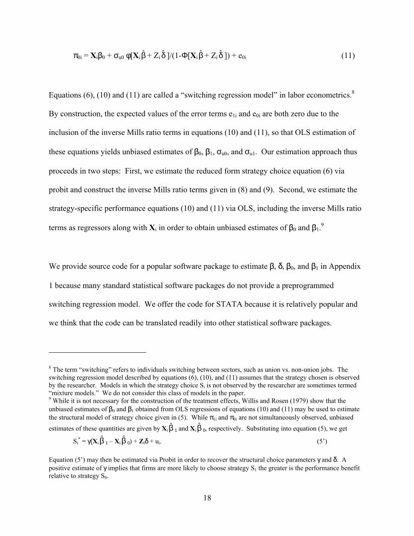
Equations (6), (10) and (11) are called a “switching regression model” in labor econometrics.8

By construction, the expected values of the error terms e1i and e0i are both zero due to the

inclusion of the inverse Mills ratio terms in equations (10) and (11), so that OLS estimation of

these equations yields unbiased estimates of β0, β1, σu0, and σu1. Our estimation approach thus

proceeds in two steps: First, we estimate the reduced form strategy choice equation (6) via

probit and construct the inverse Mills ratio terms given in (8) and (9). Second, we estimate the

strategy-specific performance equations (10) and (11) via OLS, including the inverse Mills ratio

terms as regressors along with Xi in order to obtain unbiased estimates of β0 and β1.9

We provide source code for a popular software package to estimate β, δ, β0, and β1 in Appendix

1 because many standard statistical software packages do not provide a preprogrammed

switching regression model. We offer the code for STATA because it is relatively popular and

we think that the code can be translated readily into other statistical software packages.

8 The term “switching” refers to individuals switching between sectors, such as union vs. non-union jobs. The switching regression model described by equations (6), (10), and (11) assumes that the strategy chosen is observed by the researcher. Models in which the strategy choice Si is not observed by the researcher are sometimes termed “mixture models.” We do not consider this class of models in the paper. 9 While it is not necessary for the construction of the treatment effects, Willis and Rosen (1979) show that the unbiased estimates of β0 and β1 obtained from OLS regressions of equations (10) and (11) may be used to estimate the structural model of strategy choice given in (5). While π1i and π0i are not simultaneously observed, unbiased estimates of these quantities are given by Xi 1 and Xiβ 0, respectively. Substituting into equation (5), we get β̂ ˆ

Si* = γ(Xi 1 – Xiβ 0) + Ziδ + ui. (5’) β̂ ˆ

Equation (5’) may then be estimated via Probit in order to recover the structural choice parameters γ and δ. A positive estimate of γ implies that firms are more likely to choose strategy S1 the greater is the performance benefit relative to strategy S0.

18

The implications of the estimated covariance terms σu1 and σu0 are often ignored in strategy

research, yet they can provide important insights into the types of firms that choose strategy S1 or

strategy S0. Consider, for example, the case when σu1 < 0. Recall that the expected performance

for those firms observed to choose strategy S1 is E(π1i| S1) = Xiβ1 - σu1 φ[Xi β̂ +i δ̂ ]/Φ[Xi β̂ +

Zi δ̂ ]. Because the inverse Mills ratio is always positive in the binary strategy choice case (it is a

density function divided by a distribution function), σu1 < 0 means that E(π1i| S1) > Xiβ1. This

inequality implies positive selection into strategy S1. If all firms in the sample were forced to

adopt S1, the average performance (for firms with characteristics Xi) would be given by Xiβ1.

However, when σu1 < 0, firms actually choosing S1 have above average performance using this

strategy. If firms that chose S0 had in fact chosen S1, their performance would have been worse

than that of firms actually choosing S1, i.e., E(π1i| S1, Xi) > E(π1i| S0, Xi). Conversely, when σu1

> 0, there is negative selection into strategy S1. In this case, firms actually choosing S1 have

below average performance. If the firms choosing S0 had chosen S1 instead, their performance

would have exceeded that of the observed S1 firms.

In the case where σu0 > 0, note that E(π0i |S0) = Xiβ0 + σu0 φ[Xi β̂ + Zi δ̂ ]/(1-Φ[Xi β̂ + Zi δ̂ ]), so

that E(π0i| S0) > Xiβ0 and we have positive selection into strategy S0. In this case, if S1 firms had

instead chosen S0, their performance would have been worse than that of firms actually choosing

S0. In other words, E(π0i| S0, Xi) > E(π0i| S1, Xi). If σu0 < 0, there is negative selection into

strategy S0 and E(π0i| S0, Xi) < E(π0i| S1, Xi).

19

Considering the two covariance terms together, we can construct a taxonomy of strategy choice

and performance. If σu1 < 0 and σu0 > 0, we have what may be termed a situation of comparative

advantage (Maddala 1983): firms that choose strategy S1 have above average performance using

this strategy, and firms choosing strategy S0 also have above average performance using their

chosen strategy. Firms therefore choose the strategy that provides them with a relative

advantage. For example, firms choosing to make (S1) may have production capabilities that

increase their performance only if they choose to make, while the unobserved production

capabilities of firms choosing to buy (S0) may be valuable only if they buy.

If σu1 < 0 and σu0 < 0, firms that actually choose S1 would have above average performance

regardless of whether they adopt strategy S1 or S0, since there is positive selection into strategy

S1 and negative selection into strategy S0. The S1 firms thus possess an absolute advantage:

Firms choosing S0 have below average performance regardless of the strategy chosen.

Continuing our example, suppose unobserved production capabilities enhance performance

regardless of whether the firm makes or buys, and firms choosing to make have higher levels of

this capability. These firms would have absolute advantage, since they would be higher

performers regardless of whether they chose to make or buy. If σu1 > 0 and σu0 > 0, the S0 firms

possess the absolute advantage so that E(π0i| S0, Xi) > E(π0i| S1, Xi) and E(π1i| S0, Xi) > E(π1i| S1,

Xi). Finally, the situation in which σu1 > 0 and σu0 < 0 suggests that firms choose the strategy in

which they have a comparative disadvantage. This situation should rarely occur in practice,

since all firms would be choosing a strategy that yields poorer performance than the alternative.

Such results may indicate model mis-specification, or perhaps regulatory or other factors that

force firms to choose a less profitable strategy. When σu1 = σu0 = 0, firms have no unobservable

20

advantage or disadvantage and thus endogeneity bias is not a concern. Put differently,

endogeneity bias is a concern only when firms have some unobservable (to the researcher)

advantage or disadvantage that influences the strategy they choose.

Treatment effects with endogenous treatment (Strategy effects with endogenous choice of

strategy). The estimated parameters from equations (10) and (11) may be used to construct a

variety of treatment effects. The average treatment effect (Rubin 1974, 1978; Heckman and

Robb 1985) for a firm with characteristics Xi is given by

E(π1 - π0| Xi) = Xi(β1 - β0) (12)

This treatment effect answers the question: What is the effect on performance of strategy S1 vs.

S0 for a randomly selected firm from the population of firms with characteristics Xi? This is the

treatment effect typically estimated in the strategy literature.

While informative, there may be other questions of interest regarding strategy and performance

that cannot be answered by the average treatment effect. For example, one might ask the

question: What gain in performance did S1 firms achieve by following this strategy rather than

S0? This question may be answered by constructing what the literature calls the treatment effect

for the treated (Rubin 1974, 1978; Heckman and Robb 1985), which is the performance benefit

realized for those firms that chose S1 and is constructed conditional upon the choice of strategy:

E(π1 - π0| S1, Xi) = Xi(β1 - β0) + (-σu1 + σu0)φ[Xi β̂ + Zi δ̂ ]/Φ[Xi β̂ + Zi δ̂ ] (13)

The first term on the right-hand side of (13) is the average treatment effect. The second term on

the right-hand side accounts for the fact that we are conditioning on strategy choice, in this case

S1. The second term thus incorporates the information that firms self-select into strategy S1, and

21

so may differ from a randomly selected firm in the population. Note that if there is a situation of

comparative advantage, the second term is positive, implying that the treatment effect for the

treated for firms choosing S1 is greater than the average treatment effect. Consequently, the

average treatment effect will understate the performance gain from strategy S1 among firms

adopting S1. Conversely, if the environment is characterized by absolute advantage, the average

treatment effect may be greater or less than the treatment effect for the treated, depending on the

relative magnitudes of σu1 and σu0. If there is no selection bias, so that σu1 = σu0 = 0, then

equations (12) and (13) show that the average treatment effect and the treatment effect for the

treated coincide.

An expression similar to (13) can be constructed to estimate the treatment effect for the treated

for firms choosing strategy S0 (that is, the performance benefit realized for those firms that chose

S0):

E(π1 - π0| S0, Xi) = Xi(β1 - β0) + (σu1 - σu0)φ[Xi β̂ + Zi δ̂ ]/(1 - Φ[Xi β̂ + Zi δ̂ ]) (14)

Again, the second term on the right hand side of (14) accounts for the possibility that the subset

of firms choosing strategy S0 may differ in some unobserved (by the researcher) way from other

firms in the market. Equation (14) may be used to answer the question: Could firms that chose

strategy S0 have improved their performance by choosing strategy S1?

Estimation Issues. Two major issues arise when estimating the endogenous switching regression

model defined by equations (6), (10), and (11). The first concerns the assumption that the error

terms in these equations are jointly normally distributed, while the second concerns the

identification of the model parameters. The model may be sensitive to departures from

22

normality so that the estimates are fragile and potentially biased (Little 1985). Evaluating

normality requires appealing to a number of alternative approaches that have been suggested to

deal with this problem. The researcher may transform the dependent variable (e.g., use the

natural logarithm) in order to make the performance variables look more “normal”. The research

may also adopt an alternative distributional assumption, such as the multivariate-t, for the error

terms. Heckman and MaCurdy (1986) provide formulae for the inverse Mills ratio functions for

many alternative distributions. Chib and Hamilton (2000) show that in many cases, multivariate-

t or a mixture of normal distributions provide a robust specification. Finally, there are non-

parametric alternatives, such as including squares and higher order powers of the inverse Mills

ratios in equations (10) and (11) to account for potential non-normality (see Lee 1982; Newey

1988). Unfortunately, these more robust specifications often come at the cost of a more difficult

interpretation of the parameters.

Perhaps the more important issue in the estimation of the endogenous switching regression

model concerns identification. Our specification of the reduced form strategy choice in equation

(6) suggests that the researcher has one or more instrumental variables Zi that affect strategy

choice but do not directly impact performance (i.e., they do not directly enter the performance

equations (10) and (11)). In the absence of such instrumental variables, the inverse Mills ratio

terms in (10) and (11) are simply non-linear functions of Xi, so that the parameters σu1 and σu0

are only identified by the normality functional form assumption. It is well known that

identification by functional form alone in this model often leads to very unstable and unreliable

estimates of the parameters (Little 1985). Note also that if strategy choice is a function of

23

expected performance (as it is likely to be), all the variables that affect performance should be

included in the strategy choice probit model.

Unfortunately, it is difficult in many strategy data sets to find instrumental variables that affect

strategy choice but not performance. In some cases, one might look for variables associated with

government policies that change over time or differ across localities that impact the cost of

adopting particular strategies. For instance, deregulation of the airline and trucking industries or

state level regulations that vary by state offer potential instruments if they affect strategic choices

of interest but are unlikely to directly affect performance. Alternatively, but less satisfactorily,

are firm-specific covariates that have high adjustments costs (i.e., are more inert and slow

changing) compared to the focal management decisions and that affect strategy choice but not

performance. In the absence of these instruments, it is difficult to account for endogenous

strategy choice. The best the researcher may be able to do is to account for as much of the

observable differences between firms adopting strategies S1 and S0 as possible by estimating the

exogenous treatment model given by equations (2) and (3) with a sufficiently rich specification

of the observable characteristics vector Xi (e.g., include polynomial transformations and

interactions between variables). Of course, the researcher should acknowledge the potential for

bias induced by unobserved factors.

A similar approach is to match the S1 and S0 by the firms’ predicted probability of adopting

strategy S1, generated from the probit model in (6). For matched S1 and S0 observations (i.e.,

those observations with the same or similar predicted probabilities of adopting S1), one can then

calculate the difference in performance outcomes π1 - π0 to construct a measure of the treatment

24

effect. This “propensity score matching” approach has been used in biostatistics and more

recently in economics to account for as much of the observable (by the researcher) differences

across firms that adopt different strategy choices as possible (see Rosenbaum and Rubin (1983)

for more details). It should be emphasized that these approaches do not account for unobserved

factors that affect both strategy choice and performance, and so they are still subject to selection

bias. However, they may provide a second-best estimation approach when appropriate

instruments are not available.

Multiple strategies and continuous performance

The estimation approach outlined in the endogenous switching regression model above can be

extended to situations in which more than two strategies or organizational choices are available.

We consider first the situation in which strategies may be ordered.10 For example, firms may

have the choice to produce internally (“make”), procure through an alliance (“ally”), and

outsource by using the market (“buy”). The firm’s strategy choice consists of buy, ally, and

make defined as strategies S0, S1, and S2, with associated performance levels π0, π1, and π2,

respectively. Using our example, the treatment effects of interest consist of various binary

comparisons, such as the performance implications of make vs. buy (π2 - π0), ally vs. make (π1 -

π0), and buy vs. ally (π2 - π1). The estimation approach is very similar to that described above:

we first estimate the reduced form strategy choice equation, which is now an ordered probit

rather than a simple probit model. In this case, firms adopt strategy S0 if Si* < c0, adopt S1 if c0 <

Si* < c1, and adopt S2 if Si

* > c1. Estimates for the first-stage ordered Probit are used to construct

10 Idson and Feaster (1990) apply this type of model to analyze selection-corrected wage differentials between small, medium, and large firms.

25

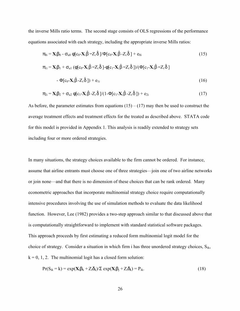
the inverse Mills ratio terms. The second stage consists of OLS regressions of the performance

equations associated with each strategy, including the appropriate inverse Mills ratios:

π0i = Xiβ0 - σu0 φ[c0-Xi β̂ −Zi δ̂ ]/Φ[c0-Xi β̂ -Zi δ̂ ] + e0i (15)

π1i = Xiβ1 + σu1 (φ[c0-Xi β̂ −Zi δ̂ ]-φ[c1-Xi β̂ −Zi δ̂ ])/(Φ[c1-Xi β̂ −Zi δ̂ ]

- Φ[c0-Xi β̂ -Zi δ̂ ]) + e1i (16)

π2i = Xiβ2 + σu2 φ[c1-Xi β̂ -Zi δ̂ ]/(1-Φ[c1-Xi β̂ -Zi δ̂ ]) + e2i (17)

As before, the parameter estimates from equations (15) – (17) may then be used to construct the

average treatment effects and treatment effects for the treated as described above. STATA code

for this model is provided in Appendix 1. This analysis is readily extended to strategy sets

including four or more ordered strategies.

In many situations, the strategy choices available to the firm cannot be ordered. For instance,

assume that airline entrants must choose one of three strategies—join one of two airline networks

or join none—and that there is no dimension of these choices that can be rank ordered. Many

econometric approaches that incorporate multinomial strategy choice require computationally

intensive procedures involving the use of simulation methods to evaluate the data likelihood

function. However, Lee (1982) provides a two-step approach similar to that discussed above that

is computationally straightforward to implement with standard statistical software packages.

This approach proceeds by first estimating a reduced form multinomial logit model for the

choice of strategy. Consider a situation in which firm i has three unordered strategy choices, Sik,

k = 0, 1, 2. The multinomial logit has a closed form solution:

Pr(Sik = k) = exp(Xiβk + Ziδk)/Σ exp(Xiβj + Ziδk) = Pik. (18)

26

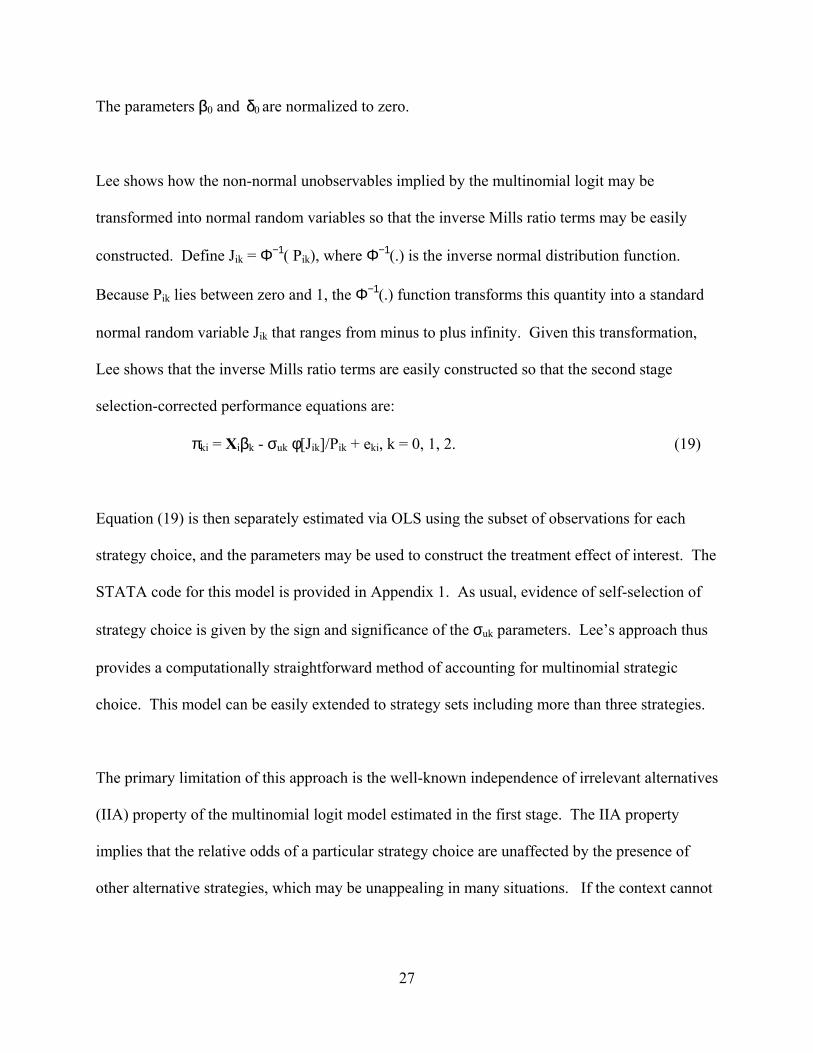
The parameters β0 and δ0 are normalized to zero.

Lee shows how the non-normal unobservables implied by the multinomial logit may be

transformed into normal random variables so that the inverse Mills ratio terms may be easily

constructed. Define Jik = Φ−1( Pik), where Φ−1(.) is the inverse normal distribution function.

Because Pik lies between zero and 1, the Φ−1(.) function transforms this quantity into a standard

normal random variable Jik that ranges from minus to plus infinity. Given this transformation,

Lee shows that the inverse Mills ratio terms are easily constructed so that the second stage

selection-corrected performance equations are:

πki = Xiβk - σuk φ[Jik]/Pik + eki, k = 0, 1, 2. (19)

Equation (19) is then separately estimated via OLS using the subset of observations for each

strategy choice, and the parameters may be used to construct the treatment effect of interest. The

STATA code for this model is provided in Appendix 1. As usual, evidence of self-selection of

strategy choice is given by the sign and significance of the σuk parameters. Lee’s approach thus

provides a computationally straightforward method of accounting for multinomial strategic

choice. This model can be easily extended to strategy sets including more than three strategies.

The primary limitation of this approach is the well-known independence of irrelevant alternatives

(IIA) property of the multinomial logit model estimated in the first stage. The IIA property

implies that the relative odds of a particular strategy choice are unaffected by the presence of

other alternative strategies, which may be unappealing in many situations. If the context cannot

27

support the IIA property then one must implement more complicated simulation methods.11 For

instance, Geweke, Keane, and Runkle (1994) describe simulation approaches for estimating the

multinomial probit model, which does not impose the IIA property. Unfortunately, these

methods are not readily implemented in standard econometric software packages and thus are

beyond the scope of our presentation.

As a final comment to this section we note that all of the models developed so far account for

endogeneity in the context of a set of discrete strategy or organizational choices. In some

instances, the strategy set may be continuous, which calls for instrumental variable techniques

like two- and three- stage least squares. Since these methods are now standard they are not

reviewed here.

Panel data

The availability of longitudinal data on strategy choices and performance may allow the

researcher to recover treatment effects of interest under less stringent assumptions than those

described above. For instance, panel data may omit the need for an instrumental variable or may

give better information about how a firm performs under different strategy regimes.

Nonetheless, as we discuss below, simple panel data models of the type generally found in the

literature have implicit assumptions of their own that may not hold for many questions of interest

11 Another complication also is possible. The researcher could be interested in analyzing different sets of strategic choices. For instance the firm may be choosing whether to make or buy, and whether to join a network. In this case, the firm has two separate strategic decisions to make. If choices are uncorrelated, then one can estimate two separate probit regressions for the two decisions and then construct the inverse Mills ratio terms in the usual way. Because there are four possible combinations of strategies, the second step consists of estimating the four performance regressions corresponding to each strategy combination (e.g., make and join a network) including the appropriate inverse Mills ratios. If the strategic decisions are correlated, however, more complicated models are necessary since the first step requires the estimation of a multivariate probit model, and the inverse Mills ratios for the second stage are much more complicated functions (see Maddala (1983) for further details).

28

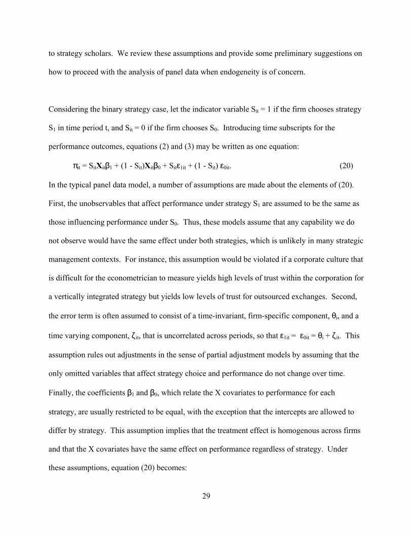
to strategy scholars. We review these assumptions and provide some preliminary suggestions on

how to proceed with the analysis of panel data when endogeneity is of concern.

Considering the binary strategy case, let the indicator variable Sit = 1 if the firm chooses strategy

S1 in time period t, and Sit = 0 if the firm chooses S0. Introducing time subscripts for the

performance outcomes, equations (2) and (3) may be written as one equation:

πit = SitXitβ1 + (1 - Sit)Xitβ0 + Sitε1it + (1 - Sit) ε0it. (20)

In the typical panel data model, a number of assumptions are made about the elements of (20).

First, the unobservables that affect performance under strategy S1 are assumed to be the same as

those influencing performance under S0. Thus, these models assume that any capability we do

not observe would have the same effect under both strategies, which is unlikely in many strategic

management contexts. For instance, this assumption would be violated if a corporate culture that

is difficult for the econometrician to measure yields high levels of trust within the corporation for

a vertically integrated strategy but yields low levels of trust for outsourced exchanges. Second,

the error term is often assumed to consist of a time-invariant, firm-specific component, θi, and a

time varying component, ζ it, that is uncorrelated across periods, so that ε1it = ε0it = θi + ζ it. This

assumption rules out adjustments in the sense of partial adjustment models by assuming that the

only omitted variables that affect strategy choice and performance do not change over time.

Finally, the coefficients β1 and β0, which relate the X covariates to performance for each

strategy, are usually restricted to be equal, with the exception that the intercepts are allowed to

differ by strategy. This assumption implies that the treatment effect is homogenous across firms

and that the X covariates have the same effect on performance regardless of strategy. Under

these assumptions, equation (20) becomes:

29

πit = γSit + Xitβ + θi + ζ it. (21)

In practice, the time-invariant error term θi is generally treated as a firm-specific random effect

or fixed effect. One difficulty with the random effect specification is the assumption that the

firm-specific effect θi is uncorrelated with the observed covariates, Sit and Xit. This

specification rules out the existence of time-invariant unobserved factors that effect both strategy

choice and performance, which is precisely the endogeneity of strategy choice for which we are

trying to account. Conversely, the fixed effect specification allows θi to be correlated with Sit

and Xit. Firm fixed effects are incorporated into the model by either including a set of firm

indicator variables into the regression, or differencing (21) in order to eliminate the time-

invariant components. For instance, the first difference of equation (21) is given by:

πit - πit-1 = γ(Sit - Sit-1) + (Xit - Xit-1)β + (ζ it - ζ it-1) (22)

Under the assumptions outlined below, estimating (22) via OLS yields a consistent estimate of

the treatment effect γ, since θi is eliminated from the regression.

Specification (22) provides a convenient method of estimating the impact of strategy on

performance, accounting for unobserved firm characteristics that may be correlated with strategy

choice. However, this specification also involves a number of implicit assumptions that may not

be appropriate for some strategic management research. First, equation (22) assumes that the

effect of strategy on performance is homogeneous across firms, so that γ measures the average

treatment effect, which is assumed to be equal to the treatment effect for the treated. Second,

equation (22) assumes that the unobservables have the same impact on performance under both

S1 and S0, which would not be the case in our prior illustration of the effect of corporate culture

30

on performance for two different organizational strategies. Third, γ is identified by within-firm

changes in strategy over time. If each firm’s strategy choice does not vary over the course of the

panel, γ cannot be estimated from (22) (in fact, only the impact of the time-varying components

of Xit can be estimated). More importantly, (22) implies that changes in strategy choice are

exogenous (Jakubson 1991). However, this raises the question of why the firm changed its

strategy choice during the panel data period. It seems reasonable to expect in many cases that

changes in unobserved (by the researcher) factors lead the firm to change its strategy and also

directly affect performance. The estimated value of γ may be biased if this is true.

When unobservables affecting strategy choice and performance change over time, or have

different impacts on performance depending on the strategy adopted, the researcher may

consider longitudinal versions of the switching regression model described by equations (6), (10)

and (11). Suppose that the error terms in equation (20) consist of a time-invariant, sector specific

random component and an independent period-specific disturbance, so that they may be written

as ε0it = θ0i + ζ0it and ε1it = θ1i + ζ1it. If one assumes that there are no time-invariant effects in

either sector, so that θ0i = θ1i = 0, then one can treat the longitudinal data on the same firm as

independent observations, and simply estimate a pooled version of the model given by equations

(6), (10), and (11). However, such an independence assumption seems extremely restrictive,

since unobserved firm-level factors are likely to evolve slowly over time. To account for such

time-invariant, unobserved firm-level factors using the two-step approach, one must develop

expressions for the E(θ0i + ζ0it| Sit = 0) and E(θ1i + ζ1it| Sit = 1) selection correction terms.

Unfortunately, without strong assumptions, these expectation terms cannot be written as simple

closed form expressions similar to the inverse Mills ratio terms in (8) and (9), and thus cannot

31

easily be implemented using standard software packages. Studies such as Wooldridge (1995,

2002), Vella and Verbeek (1998), and Dustmann and Rochina-Barrachina (2000) describe how

to construct selection-correction terms for the panel data selection model, while studies such as

Chib and Hamilton (2000, 2001) describe simulation-based econometric approaches. We refer

the reader to these papers for further discussion of how alternative panel data models may be

estimated for this problem.

Conclusion

Endogeneity should be a central concern to empirical researchers in the field of strategic

management. Indeed, it can be argued that endogenous self-selection, which equates to the view

that managers choose strategies and organizational forms with the expectation that they will

yield high performance, is the underpinning of our field. All strategic management studies

investigating the performance implications of choosing alternative strategies, whether these

strategies are discrete and finite in number or continuous and infinite in number, need to be

concerned with potential biases in coefficient estimates due to endogeneity. However, despite

the fact that basic empirical techniques accounting for omitted variables and endogenous self-

selection have been available for almost two decades, and even though the past decade has seen a

sea change in empirical methods toward the use of econometric techniques, only recently have

some of these empirical techniques begun to make their way into papers published SMJ. This

paper attempted to overcome two factors that may contribute to delays in applying these

techniques for discrete strategy choices more widely in strategic management research:

opaqueness in prior technical presentations and the lack of pre-programmed methods in

econometrics packages. The techniques described in this paper are no longer difficult to

32

implement in standard econometric packages, yet the payoff from using them is likely to be

great. More widespread use of corrections for endogeneity may yield both more accurate

estimates of the costs and benefits of alternative strategic choices (e.g., Masten 1996) as well as

reconcile mixed empirical findings in the literature (e.g., Capon et al. 1990, Shaver 1998)

concerning the performance outcomes of strategic decision-making. We hope that our

presentation helps to hasten the application of these techniques to strategic management

research, which we believe, may fundamentally advance and possibly redirect the field.

33

Bibliography

Capon, N., Farley, J.U. and Hoenig, S. (1990) ‘Determinants of Financial Performance: A Meta-Analysis’, Management Science 36 (October): 1143-2259.

Chib, S. and Hamilton, B. H. (2000) ‘Bayesian Analysis of Cross-Section and Clustered Data Treatment Models’, Journal of Econometrics 97(1): 25-50

__________ (2001) ‘Semiparametric Bayes Analysis of Longitudinal Data Treatment Models’, mimeo, John M. Olin School of Business.

Dustmann, C. and Rochina-Barrachina, M. (2000) ‘Selection Correction in Panel Data Models: An Application to Labour Supply and Wages’, IZA Discussion Paper 162.

Geweke, J., M. Keane, and Runkle, D. (1994) ‘Alternative Computational Approaches to Inference in the Multinomial Probit Model’, Review of Economics and Statistics 76: 609-632.

Greene, W. (1981) ‘Sample Selection bias as a Specification Error: Comment’, Econometrica 49: 795-798.

Heckman, J. (1974) ‘Shadow Prices, Market Wages, and Labor Supply’, Econometrica 42: 679-694.

__________ (1979) ‘Sample Selection Bias as a Specification Error’, Econometrica 47: 153-161.

Heckman, J. and MaCurdy, T. (1986) ‘Labor Econometrics’, in Z. Grilliches and M. Intrilligator (eds) Handbook of Econometrics, New York: North-Holland Publishing.

Heckman, J. J. and Robb Jr., R. (1985) ‘Alternative Methods for Evaluating the Impact of Interventions: An Overview’, Journal of Econometrics 30(n1-2): 239-67.

Idson, T. and Feaster, D. (1990) ‘A Selectivity Model of Employer-Size Wage Differentials’, Journal of Labor Economics 8: 99-122.

Jakubson, G. (1991) ‘Estimation and Testing of Union Wage Effects Using Panel Data’, Review of Economic Studies 58: 971-991.

Lee, L.F. (1978) ‘Unionism and Wage Rates: A Simultaneous Equation Model with Qualitative and Limited (Censored) Dependent Variables’, International Economic Review 19: 415-433.

__________ (1982) ‘Some Approaches to the Correction of Selectivity Bias’, Review of

Economic Studies 49: 355-72.

34

Little, R. (1985) ‘A Note About Models for Selectivity Bias’, Econometrica 53: 1469-1474.

Maddala, G.S. (1983) Limited-Dependent and Qualitative Variables in Econometrics. Cambridge: Cambridge University Press.

Masten, S. E. (1993). ‘Transaction Costs, Mistakes, and Performance: Assessing the Importance of Governance’, Managerial and Decision Economics 14: 119-129.

Murphy, K. and Topel, R. (1985) ‘Estimation and Inference in Two-Step Econometric Models,’ Journal of Business and Economic Statistics 3: 370-379.

Masten, S. E. (1996) ‘Empirical Research and Transaction Cost Economics: Challenges, Progress, Directions’, in J. Grownewegen (ed) Transaction Cost Economics and Beyond, pp. 43-64. Boston MA: Kluwer Academic Publishers.

Newey, W. (1988) ‘Two Step Series Estimation of Sample Selection Models’, mimeo, Princeton University.

Roy, A. D. (1951) ‘Some Thoughts on the Distribution of Earnings’, Oxford Economic Papers 3: 135-46.

Rosenbaum, P. R. and Rubin, D. B. (1983) ‘The Central Role of the Propensity Score in Observational Studies for Causal Effects’, Biometrika 70: 41-55.

Rubin, D. (1974) ‘Estimating Causal Effects of Treatments in Randomized and Nonrandomized Studies’, Journal of Educational Psychology 66: 688-701.

__________ (1978) ‘Bayesian Inference for Causal Effects’, The Annals of Statistics 6: 34-58.

Shaver, J. M. (1998) ‘Accounting for Endogeneity When Assessing Strategy Performance: Does Entry Mode Choice Affect FDI Survival?’ Management Science 44(4): 571-585.

Vella, F. (1998) ‘Estimating Models with Sample Selection Bias: A Survey’, Journal of Human Resources XXXIII: 127-169.

Vella, F. and Verbeek, M. (1998) ‘Whose Wages Do Unions Raise? A Dynamic Model of Unionism and Wage Rate Determination for Young Men’, Journal of Applied Econometrics 13: 163-183.

Wooldridge, J. (1995) ‘Selection Corrections for Panel Data Models Under Conditional Mean Independence Assumptions’, Journal of Econometrics 68: 115-132.

_______. (2002) Econometric Analysis of Cross Section and Panel Data. Cambridge MA: MIT Press.

Willis, R. and Rosen, S. (1979) ‘Education and Self-Selection’, Journal of Political Economy, 87 (Supplement): S7-S36.

35

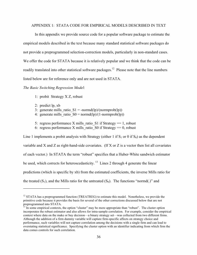
APPENDIX 1: STATA CODE FOR EMPIRICAL MODELS DESCRIBED IN TEXT

In this appendix we provide source code for a popular software package to estimate the

empirical models described in the text because many standard statistical software packages do

not provide a preprogrammed selection-correction models, particularly in non-standard cases.

We offer the code for STATA because it is relatively popular and we think that the code can be

readily translated into other statistical software packages.12 Please note that the line numbers

listed below are for reference only and are not used in STATA.

The Basic Switching Regression Model:

1: probit Strategy X Z, robust 2: predict lp, xb 3: generate mills_ratio_S1 = -normd(lp)/(normprob(lp)) 4: generate mills_ratio_S0 = normd(lp)/(1-normprob(lp)) 5: regress performance X mills_ratio_S1 if Strategy == 1, robust 6: regress performance X mills_ratio_S0 if Strategy == 0, robust

Line 1 implements a probit analysis with Strategy (either 1 if S1 or 0 if S0) as the dependent

variable and X and Z as right-hand-side covariates. (If X or Z is a vector then list all covariates

of each vector.) In STATA the term “robust” specifies that a Huber-White sandwich estimator

be used, which corrects for heteroscedasticity. 13 Lines 2 through 4 generate the linear

predictions (which is specific by xb) from the estimated coefficients, the inverse Mills ratio for

the treated (S1), and the Mills ratio for the untreated (S0). The functions “normd(.)” and

12 STATA has a preprogrammed function (TREATREG) to estimate this model. Nonetheless, we provide the primitive code because it provides the basis for several of the other corrections discussed below that are not preprogrammed into STATA. 13 In some empirical contexts, the option “cluster” may be more appropriate than “robust”. The cluster option incorporates the robust estimator and also allows for intra-sample correlation. For example, consider the empirical context where data on the make or buy decision—a binary strategy set—was collected from two different firms. Although the addition of a firm dummy variable will capture firm-specific affects on strategy choice and performance, such variables will not capture correlation among the decisions with a single firm and can lead to overstating statistical significance. Specifying the cluster option with an identifier indicating from which firm the data comes controls for such correlation.

36

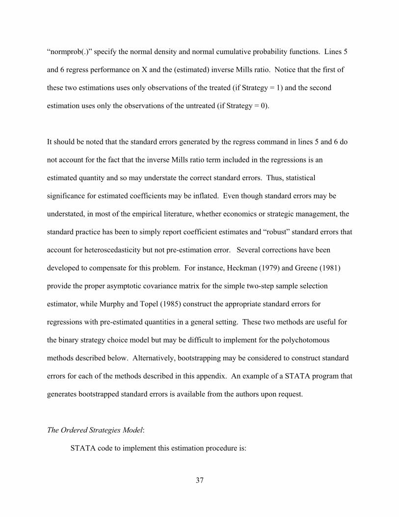
“normprob(.)” specify the normal density and normal cumulative probability functions. Lines 5

and 6 regress performance on X and the (estimated) inverse Mills ratio. Notice that the first of

these two estimations uses only observations of the treated (if Strategy = 1) and the second

estimation uses only the observations of the untreated (if Strategy = 0).

It should be noted that the standard errors generated by the regress command in lines 5 and 6 do

not account for the fact that the inverse Mills ratio term included in the regressions is an

estimated quantity and so may understate the correct standard errors. Thus, statistical

significance for estimated coefficients may be inflated. Even though standard errors may be

understated, in most of the empirical literature, whether economics or strategic management, the

standard practice has been to simply report coefficient estimates and “robust” standard errors that

account for heteroscedasticity but not pre-estimation error. Several corrections have been

developed to compensate for this problem. For instance, Heckman (1979) and Greene (1981)

provide the proper asymptotic covariance matrix for the simple two-step sample selection

estimator, while Murphy and Topel (1985) construct the appropriate standard errors for

regressions with pre-estimated quantities in a general setting. These two methods are useful for

the binary strategy choice model but may be difficult to implement for the polychotomous

methods described below. Alternatively, bootstrapping may be considered to construct standard

errors for each of the methods described in this appendix. An example of a STATA program that

generates bootstrapped standard errors is available from the authors upon request.

The Ordered Strategies Model:

STATA code to implement this estimation procedure is:

37

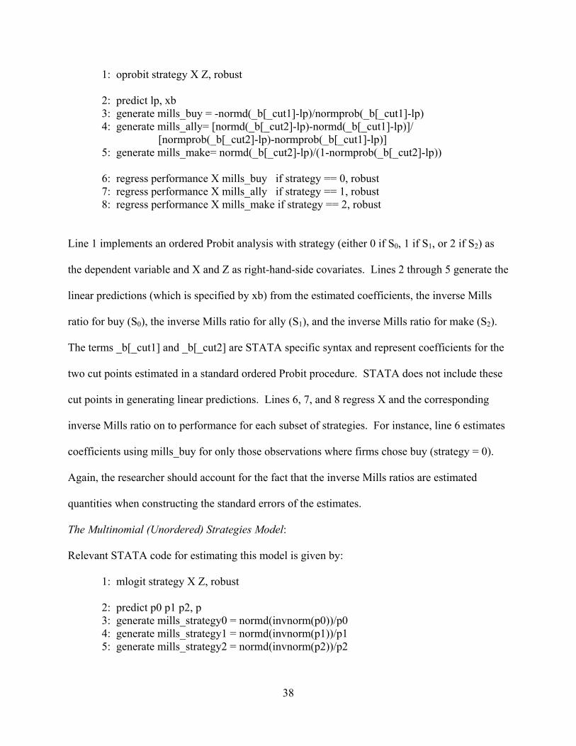
1: oprobit strategy X Z, robust 2: predict lp, xb 3: generate mills_buy = -normd(_b[_cut1]-lp)/normprob(_b[_cut1]-lp) 4: generate mills_ally= [normd(_b[_cut2]-lp)-normd(_b[_cut1]-lp)]/

[normprob(_b[_cut2]-lp)-normprob(_b[_cut1]-lp)] 5: generate mills_make= normd(_b[_cut2]-lp)/(1-normprob(_b[_cut2]-lp))

6: regress performance X mills_buy if strategy == 0, robust 7: regress performance X mills_ally if strategy == 1, robust 8: regress performance X mills_make if strategy == 2, robust

Line 1 implements an ordered Probit analysis with strategy (either 0 if S0, 1 if S1, or 2 if S2) as

the dependent variable and X and Z as right-hand-side covariates. Lines 2 through 5 generate the

linear predictions (which is specified by xb) from the estimated coefficients, the inverse Mills

ratio for buy (S0), the inverse Mills ratio for ally (S1), and the inverse Mills ratio for make (S2).

The terms _b[_cut1] and _b[_cut2] are STATA specific syntax and represent coefficients for the

two cut points estimated in a standard ordered Probit procedure. STATA does not include these

cut points in generating linear predictions. Lines 6, 7, and 8 regress X and the corresponding

inverse Mills ratio on to performance for each subset of strategies. For instance, line 6 estimates

coefficients using mills_buy for only those observations where firms chose buy (strategy = 0).

Again, the researcher should account for the fact that the inverse Mills ratios are estimated

quantities when constructing the standard errors of the estimates.

The Multinomial (Unordered) Strategies Model: Relevant STATA code for estimating this model is given by:

1: mlogit strategy X Z, robust 2: predict p0 p1 p2, p 3: generate mills_strategy0 = normd(invnorm(p0))/p0 4: generate mills_strategy1 = normd(invnorm(p1))/p1 5: generate mills_strategy2 = normd(invnorm(p2))/p2

38

6: regress performance X mills_strategy0 if strategy == 0, robust 7: regress performance X mills_strategy1 if strategy == 1, robust 8: regress performance X mills_strategy2 if strategy == 2, robust

As with the prior listing, line 1 implements the choice model of strategy (either 0 if S0, 1 if S1, or

2 if S2), in this case a multinomial logit, and X and Z as right-hand-side covariates. Line 2

generates the linear predictions; however, in this case the probability of each choice is assigned

to different variables (i.e., p0, p1, and p2). Lines 3, 4, and 5 implement Lee’s transformation to

generate the Mills ratio for each strategy. Lines 6, 7, and 8 regress X and the corresponding

inverse Mills ratio on to performance for each subset of strategies.

39

Table 1: Summary of empirical methods found in the SMJ: 1990 – 2001 1990 1991 1992 1993 1994 1995 1996 1997 1998 1999 2000 2001 count % count % count % count % count % count % count % count % count % count % count % count %

Simple Statistical Descriptors Difference in means 9 18 6 10 7 12 4 6 2 4 7 13 6 9 6 6 1 1 3 5 2 2 1 1 Correlation analysis 6 12 9 16 4 7 9 13 4 7 7 13 3 5 6 6 2 3 1 2 3 4 2 2 MANOVA 2 4 3 5 2 3 3 4 1 2 2 4 2 3 1 1 2 3 1 2 1 1 2 2 ANOVA 6 12 10 17 5 8 7 10 10 18 4 7 3 5 9 10 8 11 1 2 7 9 6 7 Variance components 1 2 1 2 0 0 2 3 0 0 0 0 2 3 2 2 1 1 1 2 0 0 2 2 Crosstab 3 6 2 3 2 3 1 1 0 0 1 2 1 2 2 2 2 3 0 0 2 2 1 1Multivariate Analysis Clustering 3 6 1 2 2 3 5 7 4 7 2 4 4 6 3 3 2 3 0 0 2 2 4 5 MDS/MDA 0 0 1 2 0 0 0 0 0 0 1 2 0 0 0 0 0 0 0 0 0 0 0 0 Factor/PCA 4 8 1 2 3 5 5 7 3 5 3 5 1 2 5 5 6 8 4 6 3 4 6 7 SEM 1 2 1 2 2 3 2 3 2 4 0 0 0 0 2 2 1 1 6 9 2 2 3 4 Meta analysis/Other 1 2 2 3 4 7 6 8 6 11 2 4 12 19 5 5 6 8 12 19 9 11 5 6Classical Regression OLS/ML 7 14 10 17 11 19 14 20 12 22 10 18 15 23 21 22 19 26 17 27 25 31 21 26 WLS 1 2 0 0 0 0 0 0 0 0 0 0 1 2 1 1 0 0 1 2 2 2 0 0 Hier. Regress 1 2 4 7 3 5 2 3 2 4 3 5 2 3 3 3 4 6 2 3 0 0 4 5 Moderated regression 0 0 1 2 1 2 2 3 1 2 3 5 0 0 1 1 2 3 3 5 0 0 0 0 SUR 0 0 0 0 0 0 0 0 0 0 0 0 0 0 0 0 0 0 0 0 0 0 0 0 GLS 0 0 2 3 0 0 2 3 1 2 2 4 0 0 2 2 1 1 2 3 2 2 3 4Limited Dep. Vars. Poisson 0 0 0 0 1 2 1 1 1 2 1 2 0 0 0 0 0 0 2 3 3 4 3 4 Tobit 0 0 0 0 0 0 0 0 0 0 0 0 0 0 1 1 2 3 0 0 0 0 0 0 Negative binomial 0 0 0 0 0 0 0 0 1 2 0 0 0 0 0 0 1 1 1 2 2 2 1 1 Logistic Binomial/ Poisson 1 2 1 2 1 2 2 3 1 2 4 7 4 6 6 6 4 6 2 3 4 5 1 1 Logit/Probit 1 2 2 3 3 5 0 0 3 5 2 4 2 3 4 4 3 4 1 2 3 4 5 6 Event history 2 4 1 2 3 5 4 6 0 0 2 4 5 8 9 10 4 6 1 2 5 6 4 5Accounts for Omitted Variables IV 0 0 0 0 1 2 0 0 0 0 0 0 1 2 0 0 0 0 0 0 1 1 0 0 FE 0 0 0 0 1 2 0 0 0 0 0 0 0 0 2 2 1 1 1 2 2 2 4 5 Endogeneity Models 0 0 0 0 3 5 0 0 1 2 0 0 0 0 3 3 0 0 2 3 1 1 3 4Total 49 100 58 100 59 100 71 100 55 100 56 100 64 100 94 100 72 100 64 100 81 100 81 100Number of papers 44 50 51 51 49 42 54 53 55 49 55 48 Number of empirical papers 26 59% 29 58% 30 59% 32 63% 31 63% 27 64% 38 70% 46 87% 41 75% 42 86% 43 78% 41 85%Methods per paper 1.9 2.0 2.0 2.2 1.8 2.1 1.7 2.0 1.8 1.5 1.9 2.0 Diversity of Methods 10 11 15 16 11 15 13 18 15 12 18 17

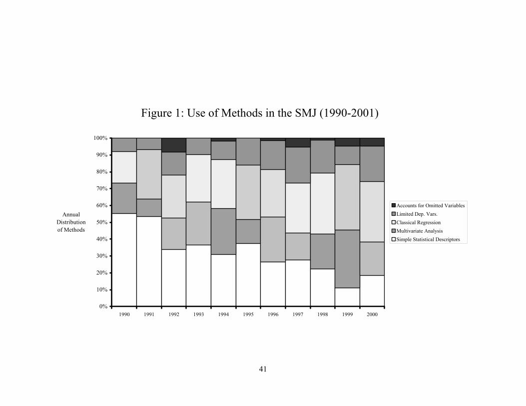
Figure 1: Use of Methods in the SMJ (1990-2001)

0%

10%

20%

30%

40%

50%

60%

70%

80%

90%

100%

1990 1991 1992 1993 1994 1995 1996 1997 1998 1999 2000

Annual Distribution of Methods

Accounts for Omitted VariablesLimited Dep. Vars.

Simple Statistical Descriptors

Classical RegressionMultivariate Analysis

41