Information Aggregation,Equilibrium Multiplicityand Market Volatility:

Morris-Shin Meets Grossman-Stiglitz

George-Marios AngeletosMIT and NBER

angelet@mit.edu

Iván WerningMIT, NBER and UTDT

iwerning@mit.edu

First draft: January 2004. This version: October 2004

Abstract

This paper argues that adding endogenous information aggregation to situationswhere coordination is important — such as currency crises, bank runs and riots — yieldsnovel insights into equilibrium multiplicity and market volatility. Morris and Shin(1998) have shown that with exogenous information multiplicity collapses when in-dividuals observe fundamentals with small enough idiosyncratic noise. In the spiritof Grossman and Stiglitz (1976), we endogenize public information by allowing indi-viduals to observe financial prices or other noisy indicators of aggregate activity. Weshow that endogenous information typically reverses the limit result: multiplicity isensured when individuals observe fundamentals with small enough idiosyncratic noise.Moreover, multiplicity may emerge with respect to assets prices in addition to regimeoutcomes. Finally, even when the equilibrium is unique, market volatilty may rise asthe exogenous noise in information is reduced.

JEL Codes: D8, E5, F3, G1.

Keywords: Multiple equilibria, coordination, self-fulfilling expectations, speculative at-tacks, currency crises, bank runs, financial crashes, rational-expectations, global games.

1

1 Introduction

It’s a love-hate relationship, economists are at once fascinated and uncomfortable with mul-

tiple equilibria. On the one hand, a variety of phenomena seem characterized by large

and abrupt changes in outcomes not obviously triggered by commensurate changes in fun-

damentals. Commentators often attribute these changes to arbitrary changes in ‘market

sentiments’ or ‘animal spirits’. Models with multiple equilibria may formally capture these

ideas. Prominent examples include self-fulfilling bank runs, currency attacks, debt crises,

financial crashes, riots and political regime changes.1 In these models multiplicity arises due

to a coordination problem: for intermediate values of the fundamentals attacking a ‘regime’

— such as a currency peg — is beneficial if and only if enough agents are also expected to

attack.

On the other hand, models with multiple equilibria are sometimes viewed as incomplete

theories that should ultimately be extended in some dimension to resolve the indeterminacy.

Recently, Morris and Shin (1998, 2000)2 have contributed to this perspective by enriching

the information structure away from common knowledge and showing that a unique equi-

librium survives when individuals observe the underlying fundamentals with small enough

idiosyncratic noise.

Their main result can be illustrated using Figure 1, where σx and σz denote the standard

deviations of the noise in private and public information regarding the fundamental.3 In

the coordination environments they consider there is multiplicity of equilibria when there is

common-knowledge of fundamentals so that either σx = 0 or σz = 0. However, for positive

levels of noise as σx becomes smaller, holding fixed σz, a unique equilibrium survives. Indeed,

in the limit as σx → 0 we approach the common-knowledge case where agents are perfectly

informed yet there is a unique equilibrium. One intuition for this uniqueness result is that

as idiosyncratic private noise decreases agents condition their actions more and more heavily

on their own private information making it harder for agents to coordinate on multiple

courses of action. The dispersion of useful information is crucial: small positive amounts of

idiosyncratic noise make agents differentially informed and imply that this information is

valuable and thus used.

The contribution of Morris-Shin is particularly attractive because it can be viewed as a

small perturbation around the original common-knowledge model and therefore as a selection

1For example, Diamond and Dybvig (1983), Obstfeld (1986, 1996), Velasco (1996), Calvo (1988), Cooperand John (1988), Cole and Kehoe (1996).

2Morris and Shin (1998) build on Carlson and van Damme (1993) who developed the Global Gamesapproach for two-player two-action games. See also Morris and Shin (1999, 2001, 2003, 2004).

3Section 2 reviews the setup that leads to this figure.

2

uniqueness

multiplicity

σz

σx

Figure 1: The Morris-Shin benchmark. σx and σz measure the noise in private and publicinformation (both exogenous). Uniqueness is ensured if σx is sufficiently small.

criterion for the latter: a unique equilibrium survives if one introduces small idiosyncratic

noise in the observation of the fundamentals. More generally, Morris-Shin provides a useful

framework for studying how the information structure affects the determinacy and charac-

terization of equilibria. As discussed above, the dispersion of valuable information regarding

fundamentals plays a critical role for the uniqueness result. An earlier literature dealt with

the transmission and aggregation of disperse information in rational-expectations equilibria.

In particular, Green (1973) and Grossman (1981) highlight that prices may be excellent ag-

gregators of dispersed information by showing that in some cases they can be fully revealing,

yielding common knowledge of economic fundamentals.

Morris-Shin abstracts from the role of financial prices and other indicators as endoge-

nous aggregators of information. Taking the information structure as exogenous is a useful

first step and helps isolate the critical role played by disperse information. However, when

financial prices convey information about the underlying fundamentals the dispersion of in-

formation is determined endogenously in equilibrium. Information aggregation can thus play

an important role in determining whether multiple equilibria arise. Indeed, Atkeson (2000)

notes that multiple equilibria may survive in the extreme case that financial prices are fully

revealing and restore common knowledge.

For many applications of these models it seems most natural to allow for public sources of

3

information that may aggregate private information, such as financial prices or other indica-

tors of economic activity. Indeed, in situations where coordination is important individuals

would find such information particularly valuable and might be expected to avidly seek them.

Also, in many economic crisis the role played by information aggregators seems to have fea-

tured prominently. For example, the Argentine crisis in late 2002 involved the abandonment

of a currency peg, sovereign-debt default, and the suspension of bank payments. Indeed,

bank deposits and the peso-forward rate deteriorated steadily throughout that year. These

variables where prominently reported in media and investor reports and it is hard to imagine

that they did not play a role in the decision economic agents were making. Similarly, during

riots and social unrest the level of others participation is surely observed to some extent and

frequently reported in the public media.

This paper investigates the implications of endogenous information aggregation in coor-

dination economies. In all cases, we avoid perfect revelation of fundamentals by allowing

enough ‘noise’ in the aggregation process, as in Grossman and Stiglitz (1976, 1980). Thus,

none of our results are driven by restoring perfect information, the main theme in Atkeson’s

comments. On the contrary, given the informational noise in the price or other indicator

of aggregate activity, a reasonable conjecture might be that uniqueness survives again when

private information is sufficiently precise. This conjecture turns out to be wrong, however,

because it ignores the endogeneity of the information structure.

When the agents’ private information regarding fundamentals becomes more precise, their

actions become more sensitive to their information. Aggregation implies that the public

indicator of others’ actions or the financial price becomes more sensitive to variations in the

underlying fundamentals. As a result, the precision of the endogenous public information is

increasing in the precision of the exogenous private information.

For the issue of multiplicity or uniqueness of equilibria a horse-race between private and

public information emerges. An increase in the precision of private information directly in-

creases the dispersion of information and therefore makes coordination harder ceteris paribus.

However, the indirect increase in the precision of public information makes coordination

easier. We show that typically the latter effect dominates the former so that endogenous

information reverses the Morris-Shin limiting result: multiplicity is ensured when individu-

als observe fundamentals with small enough idiosyncratic noise. Indeed, in this environment

uniqueness cannot be viewed as a small perturbation around common knowledge.

To illustrate our results, let σx and σz measure again the noise in private and pub-

lic information of fundamentals and let σε measure the exogenous noise introduced in the

aggregation process. The essential difference from the Morris-Shin case is that σz is now

endogenous and depends on the exogenous parameters σx and σε. Indeed, σz increases with

4

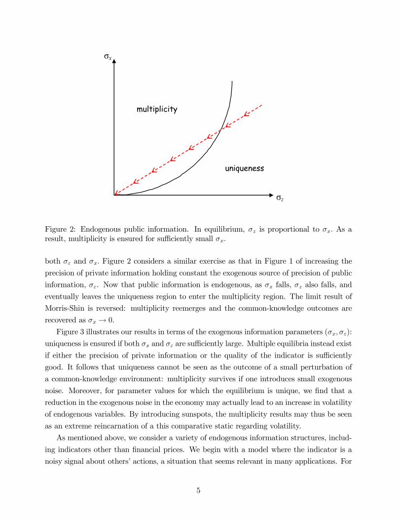
uniqueness

multiplicity

σz

σx

Figure 2: Endogenous public information. In equilibrium, σz is proportional to σx. As aresult, multiplicity is ensured for sufficiently small σx.

both σε and σx. Figure 2 considers a similar exercise as that in Figure 1 of increasing the

precision of private information holding constant the exogenous source of precision of public

information, σε. Now that public information is endogenous, as σx falls, σz also falls, and

eventually leaves the uniqueness region to enter the multiplicity region. The limit result of

Morris-Shin is reversed: multiplicity reemerges and the common-knowledge outcomes are

recovered as σx → 0.

Figure 3 illustrates our results in terms of the exogenous information parameters (σx, σε):

uniqueness is ensured if both σx and σε are sufficiently large. Multiple equilibria instead exist

if either the precision of private information or the quality of the indicator is sufficiently

good. It follows that uniqueness cannot be seen as the outcome of a small perturbation of

a common-knowledge environment: multiplicity survives if one introduces small exogenous

noise. Moreover, for parameter values for which the equilibrium is unique, we find that a

reduction in the exogenous noise in the economy may actually lead to an increase in volatility

of endogenous variables. By introducing sunspots, the multiplicity results may thus be seen

as an extreme reincarnation of a this comparative static regarding volatility.

As mentioned above, we consider a variety of endogenous information structures, includ-

ing indicators other than financial prices. We begin with a model where the indicator is a

noisy signal about others’ actions, a situation that seems relevant in many applications. For

5

uniqueness

multiplicity

σε

σx

Figure 3: Endogenous public information. σx measures the exogenous noise in private infor-mation and σε the exogenous noise in the macroeconomic indicator. Multiplicity is ensuredif either type of noise is small.

instance, during riots or bank runs, an important part of the story is that people are actively

watching what others are doing — ignoring this aspect may be missing an important piece of

the puzzle. Second, this model parsimoniously highlights aspects of the problem that recur

when financial prices are the instruments for aggregating information.

We next study environments where individuals cannot observe directly a signal about

others’ actions but instead can trade a financial asset. The asset market opens after agents

have received their private information but prior to choosing whether to attack the regime.

The rational-expectations equilibrium in the asset market generates imperfect public infor-

mation that agents can use, in addition to their private information, when deciding whether

or not to attack. This framework opens up new modeling choices regarding the specification

of the asset’s payoff and the agents’ preferences over risky returns and we consider four dif-

ferent specifications that can be solved in closed form. In all the cases considered the quality

of the public information generated by the price increases with the quality of the private

information available to the agents. This parallels the case where the public indicator was a

direct signal of others actions. Studying the asset-market environments, however, provides

novel insights.

First, we qualify our multiplicity results by presenting a case where uniqueness still

obtains in the limit as private information becomes infinitely precise. Thus, the winner

6

in the horse-race between private and public information may depend on the details of

the aggregation process. In particular, we show the importance of the sensitivity of asset

demands with respect to expected returns and the whether the asset’s dividends depends

only on exogenous fundamentals or also on endogenous variables of the coordination game.

Second, we find that multiplicity may emerge not only with respect to the probability of

regime change, but also with respect to the asset’s demand and/or price function. This occurs

only when the dividend is allowed to depend on endogenous variables of the coordination

stage and is thus a reflection of the coordination problem. Interestingly, individual’s decisions

to attack or not are then uniquely pinned down as a function of the asset price and their

private information. Thus, in these cases, the financial-market multiplicity is at the center

stage of the equilibrium multiplicity.

Finally, we consider some interesting implications for asset price volatility when the equi-

librium is unique. When the dividend depends only on economic fundamentals the volatility

of the price necessarily decreases with a reduction in either source of noise, as in Grossman-

Stiglitz. But when the dividend depends on endogenous variables from the coordination

stage a reduction in noise may increase the endogenous volatility of the coordination out-

come. This increases the volatility of the dividend and may consequently increase price

volatility. Indeed, price multiplicity may be viewed as a more extreme version of this phe-

nomena.

Related Literature

We have already discussed the relation of our work with that of Morris-Shin. Despite the

difference in results, we view our paper as underscoring the general theme emphasized by

Morris-Shin, that multiplicity or uniqueness may depend on details of the information struc-

ture and that these are worth exploring. In this respect, we stand on similar methodological

grounds as Angeletos, Pavan and Hellwig (2003, 2004), which also endogenize the informa-

tion structure, but in very different ways than the present paper — the one by considering

policy interventions and the other by considering the dynamics of coordination.

Closely related to our paper is also Mukherji, Tsyvinski and Hellwig (2004), who consider

a currency-crises game in which financial prices directly affect the central bank’s decision to

devalue in addition to aggregating information. Altough their results regarding information

aggregation alone mirror and complement our analysis in Section 4, their main contribution

is to examine how multiplicity depends on whether devaluation is triggered by large reserve

losses or high interest rates. Also, related is Tarashev (2003), who endogenizes interest

rates in the currency-crises model of Morris and Shin (1998) but does not investigate the

implications for equilibrium multiplicity.

7

The rest of the paper is organized as follows. Section 2 introduces the basic model and

reviews the Morris-Shin benchmark with exogenous public information. Section 3 introduces

endogenous public information with a signal on aggregate actions. Section 4 studies the role

of financial prices as endogenous aggregators of information. Section 5 recaps on the previous

models and focuses on their implications for market volatility.

2 The Basic Model

We present an abstract general formulation of the basic model and then briefly discuss the

various interpretations available in the literature.

Actions, Outcomes and Payoffs. There are two possible regimes, the status quo andan alternative. There is a measure-one continuum of agents, indexed by i ∈ [0, 1]. Each agentcan choose between an action that is favorable to the alternative regime and an action is

favorable to the status quo. We call these actions, respectively, “attack” and “not attack”.

All agents move simultaneously.

We denote the regime outcome with R ∈ {0, 1}, where R = 0 represents survival of the

status quo and R = 1 represents collapse. We similarly denote the action of an agent with

ai ∈ {0, 1}, where ai = 0 represents “not attack” and ai = 1 represents “attack”.

The payoff from not attacking is normalized to zero. The payoff from attacking is b > 0

if the status quo is abandoned and −c < 0 otherwise. Hence, the utility of agent i is

U(ai, R) = ai(bR − c).

Finally, the status quo is abandoned (R = 1) if and only if

A ≥ θ,

where A ≡ R aidi ∈ [0, 1] denotes the mass of agents attacking and θ ∈ R parameterizes theexogenous strength of the status quo (or the quality of the economic fundamentals).

Note that the actions of the agents are strategic complements, since it pays for an indi-

vidual to attack if and only if the status quo collapses and, in turn, the status quo collapses

if and only if a sufficiently large fraction of the agents attacks. This coordination problem

is the heart of the model.

To see the role of coordination most clearly, suppose for a moment that θ were commonly

known by all agents and let θ ≡ 0 and θ ≡ 1. For θ ≤ θ, the regime is doomed with certainty

and the unique equilibrium is every agent attacking. For θ > θ, the regime can survive an

attack of any size and the unique equilibrium is every agent not attacking. For θ ∈ (θ, θ],

8

however, the regime is sound but vulnerable to a sufficiently large attack and therefore

there are multiple equilibria sustained by self-fulfilling expectations. In one equilibrium,

individuals expect everyone else to attack, they then find it individually optimal to attack,

the status quo is abandoned, and expectations are vindicated. In another, individuals expect

no one else to attack, they then find it individually optimal not to attack, the status quo

is spared, and expectations are again fulfilled. The interval (θ, θ] thus represents the set of

“critical fundamentals” for which agents can coordinate on multiple courses of action under

common knowledge.

Interpretations. This simple model can capture the role of coordination and mul-

tiplicity of equilibria in a variety of interesting applications.4 For instance, in models of

self-fulfilling currency crises (Obstfeld, 1986, 1996; Morris and Shin, 1998), there is a cen-

tral bank interested in maintaining a currency peg and a large number of speculators, with

finite wealth, deciding whether to attack the currency or not. In this context, a “regime

change” occurs when a sufficiently large mass of speculators attacks the currency, forcing

the central bank to abandon the peg. In models of self-fulling bank runs, on the other hand,

a “regime change” occurs once a sufficiently large number of depositors decide to withdraw

their deposits, relative to liquid resources available to the system, forcing the bank to sus-

pend its payments. Other related interpretations include debt crises and financial crashes

(Calvo, 1988; Cole and Kehoe, 1996; Morris and Shin, 2003, 2004). Finally, Atkeson (2000)

interprets the model as describing riots: the potential rioters may or may not overwhelm the

police force in charge of containing social unrest depending on the number of the rioters and

the strength of the police force.

Information. When θ is common knowledge, individuals can perfectly forecast each

other actions in equilibrium and can therefore perfectly coordinate on multiple courses of

action. Following Morris and Shin (1998), we assume that θ is never common knowledge and

that individuals instead have noisy private information about θ. Private information serves

as an anchor for individual’s actions that limits the ability to forecast each others’ actions

and may therefore brake the possibility of coordinating on multiple equilibria.

Initially, nature draws θ from a distribution which constitutes the agents’ common prior

about θ. For simplicity, we let this prior be a (degenerate) uniform over the entire real line.5

4For a discussion of the defining properties and applications of regime-change games, see Angeletos,Hellwig and Pavan (2003, 2004).

5This assumption is without any serious loss of generality. At the cost of more notation and more algebra,we could easily extend the model to the case of a Normal prior. In fact, by letting the prior be uninformative,we have biased our results against multiplicity.

9

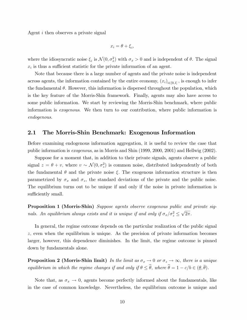
Agent i then observes a private signal

xi = θ + ξi,

where the idiosyncratic noise ξi is N (0, σ2x) with σx > 0 and is independent of θ. The signal

xi is thus a sufficient statistic for the private information of an agent.

Note that because there is a large number of agents and the private noise is independent

across agents, the information contained by the entire economy, (xi)i∈[0,1] , is enough to infer

the fundamental θ. However, this information is dispersed throughout the population, which

is the key feature of the Morris-Shin framework. Finally, agents may also have access to

some public information. We start by reviewing the Morris-Shin benchmark, where public

information is exogenous. We then turn to our contribution, where public information is

endogenous.

2.1 The Morris-Shin Benchmark: Exogenous Information

Before examining endogenous information aggregation, it is useful to review the case that

public information is exogenous, as in Morris and Shin (1999, 2000, 2001) and Hellwig (2002).

Suppose for a moment that, in addition to their private signals, agents observe a public

signal z = θ + v, where v ∼ N (0, σ2z) is common noise, distributed independently of boththe fundamental θ and the private noise ξ. The exogenous information structure is then

parametrized by σx and σz, the standard deviations of the private and the public noise.

The equilibrium turns out to be unique if and only if the noise in private information is

sufficiently small.

Proposition 1 (Morris-Shin) Suppose agents observe exogenous public and private sig-nals. An equilibrium always exists and it is unique if and only if σx/σ2z ≤

√2π.

In general, the regime outcome depends on the particular realization of the public signal

z, even when the equilibrium is unique. As the precision of private information becomes

larger, however, this dependence diminishes. In the limit, the regime outcome is pinned

down by fundamentals alone.

Proposition 2 (Morris-Shin limit) In the limit as σx → 0 or σz →∞, there is a unique

equilibrium in which the regime changes if and only if θ ≤ bθ, where bθ = 1− c/b ∈ (θ, θ).

Note that, as σx → 0, agents become perfectly informed about the fundamentals, like

in the case of common knowledge. Nevertheless, the equilibrium outcome is unique and

10

determined only by the fundamentals. This result, to which we refer to as the Morris-Shin

limit result, is very attractive, because it suggests that a small perturbation around common

knowledge obtains a unique equilibrium.

3 Endogenous Information I: Observable Actions

We now study the case where public information is endogenous. Agents no longer receive the

public signal z as assumed in section 2.1. Instead, individuals are able to observe a public

noisy signal of the aggregate activity of other agents.

We study two versions of such a model. In the first version, contemporaneous actions

are observed with noise. Thus, our equilibrium concept is novel and unavoidably at the

crossroads of rational-expectations and game theory.

The second version, in Section 3.4, has non-simultaneous moves by dividing the popu-

lation into two groups, ‘early’ and ‘late’ movers. Individuals in the early group make their

decisions to attack or not based solely on their private information. Individuals in the late

group move and are able to observe a noisy signal of the early group’s aggregate action. This

non-simultaneous version only requires standard game-theoretic equilibrium concepts. We

show that the equilibria of this second version converge to that of the first as the size of the

early movers vanishes.

3.1 Set up and equilibrium definition

We assume that, in addition to their private information, agents can condition their behavior

on a noisy indicator of the aggregate attack:

y = s(A, ε)

where s : [0, 1]×R→ R and ε is noise N (0, σ2ε), distributed independently of the fundamen-tals θ and the idiosyncratic noise ξ. The information structure is then parameterized by the

pair of standard deviations (σx, σε).

In any symmetric equilibrium agents are distinguished solely by their information, sum-

marized by their observation of the private signal xi and the public signal y. Let a(xi, y)

denote the action chosen by such an agent. The equilibrium concept is a hybrid of a perfect

Bayesian equilibrium and a rational-expectations equilibrium:

A symmetric rational-expectations equilibrium consists of an endogenous signal y =

11

Y (θ, ε), an individual attack strategy a(x, y), and an aggregate attack A(θ, y), that satisfy:

a(x, y) = arg maxa∈[0,1]

E [ U(a,R(θ, y)) | x, y ] (1)

A(θ, y) =

Zx

a(x, y)dΦ

µx− θ

σx

¶(2)

y = s(A(θ, y), ε) (3)

for all (θ, ε, x, y) ∈ R4, where R(θ, y) = 1 if A(θ, y) ≥ θ and R(θ, y) = 0 otherwise.

Condition (1) means that a(x, y) is the optimal strategy for the agent given that regime

change occurs if and only if A(θ, y) ≥ θ, whereas condition (2) means that A(θ, y) is simply

the aggregate across agents. Of course, the aggregate public signal y must be consistent with

individual actions which gives condition (3). This is the rational-expectations feature in our

equilibrium concept.6

For reasons of tractability, we specify the signal function s as

s(A, ε) = Φ−1(A) + ε.

As we will see, this specification allows the equilibrium to preserve normality of the infor-

mation structure, which in turn permits closed-form solutions. This convenient specification

was introduced by Dasgupta (2001) in a different setup. Finally, we focus on symmetric

equilibria where the information structure is normally distributed and the strategy of the

agents is monotone in private information.7 We refer to such equilibria simply as monotone

equilibria.

3.2 Equilibrium Analysis

We now study the equilibrium conditions (1)-(3). In monotone equilibria, for any realization

of y, there exist thresholds x∗(y) and θ∗(y) such that an agent attacks if and only if x ≤ x∗(y)

and the regime changes if and only if θ ≤ θ∗(y). A monotone equilibrium is thus identified

with the triplet of mappings x∗, θ∗ and Y .

We construct the set of monotone equilibria in four steps. In Step 1, we start with an

arbitrary x∗ used by the agents and use conditions (2) and (3) to characterize the implied

6In Section 3.4, we show that our results survive in a variant of the model which avoids the simultaneityin the signal and allows for a standard game-theoretic equilibrium concept.

7As we shall see 3.4, normality of the information structure is an implication when the signal is non-simultaneous.

12

aggregate attack A, the resulting θ∗ and the possible public signals Y . In Step 2, we take

θ∗ and Y as given and use condition (1) to compute the threshold x∗∗ that is individually

optimal. In Step 3, we study the fixed point x∗ = x∗∗. Finally, in Step 4, we consider the

determinacy of Y .

Step 1. In a monotone equilibrium, a(x, y) = 1 if and only if x ≤ x∗(y), for some

function x∗. The aggregate attack is then

A(θ, y) = Φ (√αx(x

∗(y)− θ)) , (4)

where αx = σ−2x . Note that A(θ, y) is decreasing in θ so there exists a function θ∗(y) such

that A(θ, y) ≥ θ if and only if θ ≤ θ∗(y). The threshold θ∗(y) solves A(θ∗(y), y) = θ∗(y), or

equivalently

x∗(y) = θ∗(y) +1√αx

Φ−1(θ∗(y)). (5)

Equilibrium condition (3) implies that the signal must satisfy,

y =√αx [x

∗(y)− θ] + ε,

or equivalently

x∗(y)− σxy = θ − σxε. (6)

For any (θ, ε) ∈ R2, let z = eZ(θ, ε) ≡ θ − σxε and note that (6) is a relation between y and

z. Define the correspondence

Y(z) = { y ∈ R | x∗(y)− σxy = z } . (7)

In Step 4, we show that Y(z) is non-empty and examine when it is single- or multi-valued.Now take any function Y (z) that is a selection from this correspondence, i.e., such that

Y (z) ∈ Y(z) for all z, and let the signal be Y (θ, ε) = Y ( eZ(θ, ε)) = Y (θ − σxε). As we shall

see any such selection preserves normality of the information structure.

Step 2. We now map θ∗ and Y to x∗∗. Given that regime change occurs if and only if

θ ≤ θ∗(y), the expected payoff for the agent is given by

E [ U(a,R(θ, ε)) | x, y ] = a {bPr [ θ ≤ θ∗(y) | x, y ]− c} .

We thus need to consider the determination of the posterior probability Pr [ θ ≤ θ∗(y) | x, y ] .

13

The observation of y = Y (θ, ε) = Y (z) is equivalent to the observation of

Z(y) ≡ x∗(y)− σxy = θ − σxε = z

That is, it is as if the agents observe a public signal z about θ, with noise N (0, σ2xσ2ε). Recallthat each agent also observes a private signal about θ, with idiosyncratic noise N (0, σ2x). Letαx ≡ σ−2x , αε ≡ σ−2ε , and αz ≡ αxαε ≡ (σxσε)−2. Combining the two sources of informationwe conclude that the posterior of an agent is

θ | x, y ∼ N ¡δx+ (1− δ)Z(y) , α−1

¢,

where α = αx+αz is the total precision of information and δ = αx/(αx+αz) is the precision

of x relative to the total.

It follows that

Pr [θ ≤ θ∗(y) | x, y] = 1− Φ¡√

α (δx+ (1− δ)Z(y)− θ∗(y))¢.

Note that the above is monotonic in x so the agent attacks if and only if x ≤ x∗∗(y), where

x∗∗(y) solves

bPr [ θ ≤ θ∗(y) | x∗∗(y), y ] = c.

Combining the above two conditions and substituting Z(y) = x∗(y) − y/√αx, we find that

x∗∗(y) must solve

Φ

µ√α

µδx∗∗(y) + (1− δ)

µx∗(y)− 1√

αxy

¶− θ∗(y)

¶¶=

b− c

b. (8)

Step 3. In equilibrium, x∗∗ = x∗ and (8) reduces to

Φ

µ√α

µx∗(y)− θ∗(y)− 1− δ√

αx

y

¶¶=

b− c

b.

Combining the above with (5), using δ = αx/(αx + αz) and α = αx + αz, and rearranging,

we obtain:

θ∗(y) = Φ

µαz

αx + αzy +

rαx

αx + αzΦ−1

µb− c

b

¶¶, (9)

x∗(y) = θ∗(y) +1√αx

Φ−1 (θ∗(y)) , (10)

14

where αz = αxαε. Hence, for all σx and σε, the equilibrium x∗ and θ∗ are determined uniquely

and irrespectively of the selected equilibrium signal Y . Moreover, both θ∗(y) and x∗(y) are

increasing in y. Finally, θ∗(y) does not depend on σx, θ∗(y) → 1 − c/b as σε → ∞ and

θ∗(y)→ Φ(y) as σε → 0.

Step 4. We finally need to consider the equilibrium correspondence Y(z). Recall thatthis is given by the set of solutions to

x∗(y)− 1√αx

y = z.

Using (9) and (10), the above reduces to

F (y) ≡ Φ

µαz

αx + αz

y + Λ

¶+

1√αx

µ− αx

αx + αz

y + Λ

¶= z, (11)

where Λ ≡pαx/ (αx + αz)Φ−1(1− c/b). Equilibrium existence and uniqueness thus reduces

to existence and uniqueness of solution to (11).

Note that F (y) is continuous in y, and F (y) → −∞ as y → +∞, and F (y) → +∞ as

y → −∞. Thus, the correspondence Y(z) is non-empty and an equilibrium always exist. Toexamine uniqueness, we ask whether Y(z) is single-valued for all z, which is true if and onlyif F is monotonic in y. Differentiating F we obtain

F 0(y) = −√αx

αx + αz

µ1− αz√

αxφ

µαz

αx + αzy + Λ

¶¶.

It follows that the determinacy of equilibrium hinges on the ratio αz/√αx, like in the Morris-

Shin benchmark. Since maxw∈R φ(w) = 1/√2π, we have that F is decreasing in y, and

therefore Y(z) is single-valued for all z, if and only if αz/√αx ≤

√2π. If instead αz/

√αx >√

2π, there are thresholds z and z such that Y(z) takes one value for z /∈ (z, z) but threevalues for z ∈ (z, z). These thresholds are given by z = F (y) and z = F (y), where y and

y are, respectively, the lowest and highest solution with F 0(y) = 0. Unlike the Morris-Shin

benchmark, however, the ratio αz/√αx is endogenous. Using αz = αεαx, we conclude that

the equilibrium is unique if and only if αε√αx ≤

√2π.

The following proposition summarizes these results.

Proposition 3 (Morris-Shin meet Grossman-Stiglitz) A monotone equilibrium is

characterized by a triplet of mappings (Y, x∗, θ∗) such that the endogenous signal satisfies

y = Y (θ, ε), a agent attacks if and only if x ≤ x∗(y), and regime change occurs if and only

if θ ≤ θ∗(y).

15

A monotone equilibrium exists for all (σx, σε) and is unique if and only if σ2εσx ≥ 1/√2π.

If σ2εσx < 1/√2π, the equilibrium signal function Y is indeterminate, but the equilibrium

threshold functions x∗ and θ∗ remain unique and independent of the selected Y .

We conclude that the equilibrium is unique only if there is enough noise in both sources

of information, the exogenous information of the agents and the endogenous signal about

aggregate activity. Multiple equilibria survive as long as either source of information is

sufficiently precise.

Interestingly, when multiplicity arises, it is with respect to aggregate outcomes but

not with respect to individual behavior. To understand this result, consider the common-

knowledge limit (σx = σε = 0), in which case x = θ and y = Φ−1(A), so that the agent learns

θ perfectly by observing x and learns A by observing y. The agent then finds it optimal

to attack if and only if A ≥ θ, or equivalently x ≤ Φ(y). Here, the equilibrium strategy

a(x, y) for the agent is uniquely determined with x∗(y) = Φ(y). However, the equilibrium

values of A and y are not uniquely determined. Instead, for every θ ∈ (θ, θ], both A = 0

and A = 1 can be sustained in equilibrium.8 When σx and σε are non-zero, the same nature

of indeterminacy remains. The equilibrium behavior of the agent is uniquely determined for

any given observation x and y, but there can be multiple equilibrium values of A and y for

any given realization of θ and ε.

Finally, since our endogenous-information economy is different from the exogenous in-

formation economy of Morris-Shin, it is interesting that the determinacy of equilibrium in

both cases hinges on exactly the same ratio αz/√αx. However, note that, in equilibrium, the

information generated by y is equivalent to the information generated by z = Z(y) = θ−σxε.Our endogenous-information economy is thus related to an exogenous-information economy

with precision of public information given by αz = αy = αεαx. Indeed, substituting this

expression into the criterion for multiplicity from proposition, ?? that σx/σ2z >√2π, yields

the criterion for multiplicity in proposition 3, that σ2εσx < 1/√2π. As the precision of private

information becomes infinite so does the precision of public information.

3.3 Information Limits

Proposition 3 establishes that, for any given level of noise in the agents’ private information,

multiple equilibria exist if and only if the noise in the macroeconomic indicator is sufficiently

8If A = 0, then y = −∞ and x∗(y) = Φ−1(−∞) = θ, in which case all agents attack whenever θ ≤ θ andno agent attacks whenever θ > θ. If instead A = 1, then y = +∞ and x∗(y) = Φ−1(+∞) = θ, in which caseall agents attack whenever θ ≤ θ and no agent attacks whenever θ > θ. In the former case, a regime changeis triggered if and only if θ ≤ θ; in the latter, if and only if θ ≤ θ.

16

small. Intuitively, an increase in σε reduces the public information generated by the obser-

vation of y and thus reduces the ability of the market to coordinate on multiple courses of

action.

Proposition 4 (Limit σε →∞) Fix σx and let σy →∞. In the limit, the regime changes

if and only if θ ≤ bθ, where bθ ≡ 1− c/b ∈ (θ, θ).

The Morris-Shin outcome is obtained as the noise in the observation of aggregate activity

becomes arbitrarily large. This is intuitive, for in this case no information is generated by

the observation of y and the endogeneity of public information is of no importance.

Consider next the limit of the precision of agents’ private information, for given level

of noise in y. Proposition 3 establishes that, for given σε, multiple equilibria exist if and

only if σx is sufficiently small. The interval (z, z) represents the region of multiplicity and a

reduction in σx reduces z and increases z making larger the multiplicity region. Indeed, as

σx → 0 we can show that any outcome is possible for all θ ∈ (θ, θ).

Proposition 5 (Limit σx → 0) Fix σε and let σx → 0. For every θ ∈ (θ, θ), there existsan equilibrium in which the probability of regime change converges to zero, as well as an

equilibrium in which the probability of regime change converges to one.

This result stands in stark contrast to the Morris-Shin limit result in Proposition 2.

With exogenous public information a unique equilibrium survives as the noise in private

information vanishes. With endogenous public information as modeled here the multiplicity

present with common knowledge obtains as the noise in private information vanishes. The

reason is once again the endogeneity of public information: As the precision of private

information increases, the precision of public information also increases, and indeed at the

same rate, so that common knowledge is recovered in the limit.

3.4 Non-Simultaneous Signal

The analysis so far has assumed that agents can condition their decision to attack on a noisy

indicator of contemporaneous aggregate behavior. Our rational-expectations equilibrium

thus required that agents choose optimally given the observed signal and that this signal be

generated by the aggregation of individual choices. We now show that our results are robust

to a perturbation that breaks the simultaneity in the signal by introducing some simple

dynamics and therefore allows for a standard game-theoretic equilibrium concept.

The population is divided into two groups, ‘early’ and ‘late’ agents. Early agents move

first, on the basis of their private information alone. Late agents move second, on the basis

17

of their private information as well as a noisy public signal about the aggregate activity

of early agents. Neither group can observe contemporaneous activity, but late agents can

condition their behavior on the activity of early agents.

Let µ ∈ (0, 1) denote the fraction of early agents, A1 the aggregate activity of earlyagents, and A2 the aggregate activity of late agents. The regime changes if and only if

µA1+(1−µ)A2 ≥ θ. The signal generated by early agents and observed only by late agents

is given by

y1 = Φ−1(A1) + ε, (12)

where ε ∼ N (0, σ2ε) is independent of θ and ξ.

Early agents can condition their actions only on their private information, whereas late

agents can condition their actions also on y1. An equilibrium is thus characterized by a

threshold x∗1 and a pair of threshold functions x∗2(y1) and θ∗(y1) such that: an early agent

attacks if and only if x ≤ x∗1; a late agent attacks if and only if x ≤ x∗2(y1); and the regime

is abandoned if and only if θ ≤ θ∗(y1). Like in the case that the signal was simultaneous,

the aggregate size of the attack and the regime outcome depend on the particular realization

of the signal, but there is no more a fixed-point relation between the signal and the size

of the attack. As a result, only standard game-theoretic concepts are need to define the

equilibrium.

Most importantly, the main insight of the previous analysis survives: As the precision of

the private information of (early) agents increases, the precision of the public information

available to late agents also increases, indeed at the same rate. As a result, multiplicity is

once again bound to obtain for sufficiently small private noise.

Unfortunately, characterizing the equilibria of the game with non-simultaneous signal

is complicated by the fact that early agents face a double forecast problem, as they are

uncertain about both the fundamental θ and the signal y1 upon which late agents will

condition their behavior. Nevertheless, as µ → 0, the impact of early agents on the size

of the attack vanishes. In the Appendix we actually show that any equilibrium of the

benchmark simultaneous-signal game can be approximated by an equilibrium of the non-

simultaneous-signal game as µ→ 0. We conclude that our multiplicity results are robust to

non-simultaneity of the signal.

18

4 Endogenous Information II: Financial Prices

The analysis so far has assumed that agents can condition their decision to attack on a direct

indicator of aggregate activity. Instead, we now allow agents to observe a financial price,

which in equilibrium serves as an indirect indicator of the fundamentals or the aggregate

activity.

4.1 Model Set-up

We modify the environment as follows. There are two stages and we refer to stage 1 as

the ‘asset market’ and stage 2 as the ‘coordination game’. Individuals begin with given

endowments of wealth wi and exogenous private signals xi = θ + ξi, where the distribution

of wi is arbitrarty and the noise ξi is as before. In stage 1, agents trade a financial asset

whose dividend depends on the underlying fundamentals. In stage 2, agents decide whether

to attack the regime or not as in the basic model. The dividend of the asset and the regime

outcome are realized at the end of stage 2. In deciding whether to attack in stage 2, agents

can no longer condition their choice on a direct signal of the aggregate attack, but they can

now use the information revealed by the price that cleared the asset market in stage 1.

This framework opens up new modeling choices regarding the specification of the financial

asset’s dividend and the preferences over risky payoffs. We guide our choices with an eye

towards tractability: to isolate the effects of information aggregation from any direct payoff

linkages between the two stages, we assume that preferences are separable between the first-

stage portfolio choice and the second-stage attacking decision;9 and to preserve normality

of the information structure, we model stage 1 along the lines of CARA-normal framework

introduced by Grossman and Stiglitz (1976, 1980) and Hellwig (1980).

In stage 1, agents can invest their wealth either in a risk-less asset or a risky asset. The

riskless asset is in infinitely elastic supply, it costs 1 in the first stage, and it delivers 1 in the

second stage. The risky asset, on the other hand, costs p in the first stage and delivers f in

the second. The agent enjoys utility from final-stage consumption and has constant absolute

risk aversion (CARA). The payoff from the portfolio choice is thus V (c) = − exp(−γc)/γ,where c = w − pk + fk is consumption, k denotes investment in the risky asset, and γ > 0

is the coefficient of absolute risk aversion. The net supply of the risky asset is given by an

unobserved random variable ε ∼ N (0, σ2ε), which is independent of both the fundamentalsand the private noise.10 As in Grossman and Stiglitz (1976, 1980), the unobserved supply

9In one case, however, we allow the payoff of the asset to be depend on the actions taken in stage 2; seebelow.10As long as the supply is exogenous, the normalization of its mean level to zero is of course without any

19

can be interpreted as the demand of ‘noise’ traders and its role is to introduce noise in the

information revealed by financial prices about fundamentals. Finally, stage 2 is as before:

agents chose whether to attack or not, the payoff from attacking is U(a,R) = a (R− c) , and

the status quo is abandoned if and only if A > θ.

What remains to close the model is the specification of the dividend f.We are interested

in two alternatives: the case that f is determined merely by the underlying economic fun-

damentals θ; and the case f is a function of the endogenous activity A of the coordination

stage. What we wish to capture with the latter case is environments where the coordination

game is some short of an investment game: agents have the option to invest in a new sector

(or adopt a new technology), the new sector is profitable only if enough agents invest, and

the financial asset is an asset whose dividend depends on the profitability of this sector and

therefore on the aggregate investment made in this sector.

Since the information available to an agent in either stage is summarized by (x, p) ,

individual actions are contingent in (x, p) . Ssince there is a continuum of agents and the

distribution of x is centered around θ, aggregates can thus be expressed as functions of (θ, p) .

The equilibrium price, on the other hand, is a function of the exogenous state, namely (θ, ε).

We thus define

Definition 1 A rational-expectations equilibrium is a price function p = P (θ, ε), individual

strategies k(x, p) and a(x, p) for investment and attacking, and corresponding aggregates

K(θ, p) and A(θ, p), such that, in the first stage:

k(x, p) = argmaxk∈R

E [ V (k, f(θ, A), p) | x, p ] (13)

K(θ, p) =

Zx

k(x, p)dΦ

µx− θ

σx

¶(14)

K (θ, P (θ, ε)) = ε (15)

and in the second stage:

a(x, p) = arg maxa∈[0,1]

E [ U(a,R) | x, p ] , (16)

A(θ, p) =

Zx

a(x, p)dΦ

µx− θ

σx

¶, (17)

where R = 1 if A(θ, p) ≥ θ and R = 0 otherwise.

The interpretation of these conditions is straightforward. Condition (13) and (17) requires

that an agent’s investment take into account the information contained in their private

loss of generality.

20

information and prices, whereas condition (15) imposes market clearing in the asset market.

Note that (13)-(15) define a standard rational-expectations equilibrium for stage 1, whereas

(16)-(17) define a standard Perfect Bayesian equilibrium in stage 2. The equilibrium concept

for the coordination game is thus free of the fixed-point feature we had in the benchmark

model.

4.2 Exogenous Dividend

We start by considering the case that the dividend of the asset is a function of the exogenous

economic fundamentals: f = f (θ) . Since, for tractability, we need f to be Normal, we let

f (θ) = θ.

By aggregating information about the dividend in stage 1, the price generates an endoge-

nous public signal about θ. The coordination game in stage 2 is ohterwise isomorphic to

the static Morris-Shin. It follows that the coordination game admits multiple equilibria if

and only if the precision of the information conveyed by the price is sufficiently higher than

the precision of the private information of the agents. The important difference is that the

noise in the price is itself an increasing function of the noise in the private information of

the agents and the noise in the supply of the asset. When either noise is low enough, the

precision of the information conveyed by the price is sufficiently high that multiple equilibria

emerge.

Proposition 6 Suppose f = θ. There are multiple equilibrium thresholds x∗(p) and θ∗(p) if

and only if σ2εσ3x < γ2(2π)−1/2, but the equilibrium price function P (θ, ε) is always uniquely

determined.

Proof. First, consider stage 1 (the financial market). By the FOC, the optimal demand

for the asset is

k(x, p) =E[ θ | x, p ]− p

γ Var[ θ | x, p ] .

We propose that the posterior of θ conditional on x, p has mean δx+ (1− δ)p and precision

α, for some δ ∈ (0, 1) and α > 0. It follows that k(x, p) = (δα/γ) (x − p) and therefore

K(θ, p) = (δα/γ) (θ − p). In equilibrium, K(θ, p) = ε, which gives the equilibrium price as

p = P (θ, ε) = θ − γ

δαε. (18)

By implication, the observation of p is equivalent to the observation of a Normal signal about

θ with precision αp = (δα/γ)2αε. Moreover, x and p are independent and therefore δ = αx/α

and α = αx+αp. Solving for α, δ, and αp, we get α = αx(1+αxαε/γ2), δ = 1/(1+αxαε/γ

2),

21

and

αp =αεα

2x

γ2. (19)

Next, note that stage 2 is isomorphic to the Morris-Shin static game, except for the fact

that the precision of the public signal is given by (19). It follows that there are multiple

equilibrium thresholds x∗(p) and θ∗(p) if and only if αp/√αx >

√2π, or equivalently σ2εσ

3x <

γ2(2π)−1/2, which completes the proof. QED

As in our benchmark model, multiple equilibria survive as long as either noise is small

enough. In fact, whereas in the benchmark model the precision of public information in-

creased proportionally with the precision of private information, here it increases more than

proportionally, which only serves to reinforce our conclusions regarding the comparative

static and limit exercises for σx.

Unlike the benchmark model, however, the indeterminacy arises with respect to individual

strategies. The price function is always uniquely determined because the dividend is a

function of the exogenous fundamentals; and as the noise vanishes, the price converges to

the underlying dividend of the asset.

Corollary 1 As σx → 0, P (θ, ε)→ θ for all (θ, ε), in every equilibrium.

4.3 Endogenous Dividend

We now consider the case that the payoff of the asset is determined by the coordination

game: f = f(A). To retain Normality, we now let f (A) = −Φ−1(A). Hence, the asset paysmore the lower the size of the attack, which we could interpret as a situation where “attack”

means refraining form investment.

In the previous example, the price played the role of a signal for the exogenous funda-

mental θ, in which case indeterminacy emerged for individual strategies and not for the price

function. Here, the price plays the role of an anticipatory signal of the size of the attack, in

which case the strategies of the agents are uniquely determined, but the equilibrium price

function may not be.

Proposition 7 Suppose f = −Φ−1(A). There are multiple equilibrium price functions

P (θ, ε) if and only if σ2εσ3x < γ2/

√2π, but the equilibrium thresholds x∗(p) and θ∗(p) are

always uniquely determined.

The information structure and the nature of multiplicity are similar to the ones in our

benchmark model. There are, however, two differences. First, whereas in the benchmark

model the signal is simultaneous with the attack and reveals the realized attack, in the present

22

model the signal preceeds the attack and reveals the agents’ expectations about the future

attack. Second, the result that aggregates are ideterminate while individual strategies are

unique now obtains more flesh and blood: it manifests itself in the form of price multiplicity.

This is most evident in the limit as noise vanishes.

Corollary 2 There is an equilibrium in which, for all θ ∈ (θ, θ) and all ε, P (θ, ε) → −∞as σx → 0. There is also an equilibrium in which, for all θ ∈ (θ, θ) and all ε, P (θ, ε)→ +∞as σx → 0.

5 Volatility

The results on equilibrium multiplicity translate directly to results on market volatility if we

add sunspots. Indeed, the possibility that agents can condition their behavior on random

variables unrelated to the fundamentals introduces “spurious” volatility.

In the exogenous-information context of Morris-Shin, multiplicity disappears when agents

observe the fundamentals with small idiosyncratic noise. By implication, there can be no such

spurious volatility for small σx. Indeed, as σx → 0, the regime outcome becomes independent

of the aggregate noise and volatility therefore vanishes.

With endogenous information aggregation, however, the impact of noise on volatility

can be quite different. A reduction in either σx or σε may perversely increase volatility by

ensuring multiplicity and therefore introducing more spurious volatility. Indeed, for any θ

in the critical region, as either σx → 0 or σε → 0, the regime can either collapse or survive,

purely as a function of the sunspot. In this sense, volatility is maximized when the noise

vanishes.

Interestingly, the property that less noise may increase volatility does not rely the exis-

tence of multiple equilibria. In the next, we show that, even when the equilibrium is unique,

a reduction in noise may increase the sensitivity of the regime outcome to the noise and may

therefore lead to more rather than less market volatility.

5.1 Regime Volatility

Consider the model of Section 3, where agents observe a noisy signal about the aggregate

size of the attack. The equilibrium thresholds (x∗, θ∗) and the signal y satisfy the following

23

set of equations:

θ∗ = Φ

µαz

αx + αzy +

rαx

αx + αzΦ−1

µb− c

b

¶¶, (20)

x∗ = θ∗ +1√αx

Φ−1 (θ∗) , (21)

y = Φ−1 (A) =√αx (x

∗ − θ) , (22)

where αz = αxαε. Solving these three equations gives the endogenous variables (x∗, θ∗, y) as

functions of the exogenous variables (θ, ε). The solution for θ∗, in particular, satisfies11

1

αε

Φ−1 (θ∗)−√αxθ∗ = −√αxθ + ε+

√1 + αε

αε

Φ−1 (1− c/b) (23)

When the equilibrium is unique, the left-hand side is monotonic in θ∗, so that the above

defines θ∗ as a unique function of the fundamentals θ, the supply shock ε, and the parameters

(αx, αε, c, b).

To examine the comparative statics of the volatility of the regime outcome with respect

the noise structure, it is useful to normalize the supply shock. The normalized shock is

defined by eε ≡ √αεε, so that eε ∼ N (0, 1). Condition (23) then becomes1√αε

Φ−1 (θ∗)−√αεαxθ∗ = −√αεαxθ + eε+ √1 + αε

αεΦ−1 (1− c/b) . (24)

We can then identify an increase in the volatility of the regime outcome with an increase in

the sensitivity of the regime threshold θ∗ with respect to the normalized shock eε.By (24), the slope of θ∗ with respect to eε is given by the reciprocal of the following:

∂θ∗

∂eε =·1√αε

1

φ (Φ−1 (θ∗))−√αεαx

¸−1> 0

It is then immediate that, keeping θ∗ constant, an increase in either αε or αx (that is, a

reduction in either σε or σx) necessarily increases the slope ∂θ∗/∂eε. As a result, less noise

may lead to more volatility in the regime outcome.12

11To see this, substitute x∗ from (21) into (22), substitute the resulting expression for y into (20), useαz = αxαε, and rearrange.12Of course, θ∗ does not stay constant as αε or αx change. In particular, θ∗ satisfies single-crossing, it

decreases for low values of eε and increases for high values of eε. Given θ, let eε0 be the unique value of eε forwhich θ∗ stays constant with a change in αε or αx. For any eε1 and eε2 such that eε1 < eε0 < eε2, we still havethat |θ∗(eε2) − θ∗(eε2)| increases with either αε or αx. In this sense, volatility increases with a reduction innoise.It remains true, however, that, at least for intermediate values of eε,

24

5.2 Price Volatility

We next examine the comparative statics of the volatility of prices. To economize, we consider

only the CARA-normal examples of Section 4; the analysis of the risk-neutral examples is

similar. To emphasize the implications for volatility that do not derive from multiplicity, we

first focus on case that the equilibrium is unique or that there are no sunspots.

When the dividend is exogenous, we have f = θ,

p = θ − 1√αpeε,

and αp = αεα2x/γ

2. When instead the dividend is endogenous, we have f = Φ−1 (A) =√αx(θ − x∗),

p =√αx(ep− x∗) =

√αx(θ − x∗)−

rαx

αpeε,

and αp = αεα3x/γ

2. In either case, we can write the equilibrium price as the sum of the

dividend and the supply shock appropriately weighted:

p = f − ¡γσεσ2x¢eεIt is immediate then that, keeping the volatility of f constant, the volatility of the price

decreases with a reduction in either σε or σx. But what about the volatility of the dividend?

When the dividend is exogenous, the volatility of f is simply the volatility of exogenous

fundamental and is thus indeed independent of either σε or σx. Like in Grossman-Stiglitz, the

impact of noise on price volatility is thus the natural one: More noise implies more volatility.

When instead the dividend is endogenous, the volatility of f depends, not only on the

exogenous volatility of the fundamentals, but also on the endogenous volatility of the regime

outcome, namely the volatility of x∗. The latter, as we discussed before, may well increase

with a reduction in either σε or σx. As a result, the overall impact of noise on price volatility

is now ambiguous: A reduction in noise reduces the volatility of the price for any given

volatility in the dividend, but it also increases the volatility of the dividend itself. In some

cases, indeed, the second effect dominates, so that price volatility increases with a reduction

in noise.

We conclude:

Proposition 8 When the dividend is exogenous, the volatility of the price necessarily de-creases with a reduction in either σε or σx. But when the dividend depends on the coordination

outcome, a reduction in either noise may increase price volatility.

25

Our earlier results regarding the multiplicity of prices can thus be viewed as an extreme

reincarnation of the above result. When the noise is sufficiently small, volatility can be high,

not only because the dividend (and therefore the price) is very sensitive to the exogenous

noise, but also because the dividend (and therefore the price) can depend on arbitrary

sunspots.

6 Final Remarks

Building on Morris and Shin (1998) this paper introduced instruments that endogenized

the sources of public information in models where coordination is important. We modeled

public information by either: (i) a noisy signal of aggregate activity; or (ii) a financial asset’s

price that reveals information in equilibrium. An important feature of the equilibrium in all

cases is that the precision of public information is endogenous and rises with the precision

of private information.

We showed that in all but one of the six models considered this effect is strong enough

to reverse the limiting uniqueness result obtained with exogenous public information. Thus,

typically, with endogenous public information multiplicity is ensured when individuals ob-

serve fundamentals with small enough idiosyncratic noise. Conversely, uniqueness is ensured

if idiosyncratic noise is large enough.

We view the main theme in Morris-Shin as emphasizing the importance of the details

of the information structures for the multiplicity or uniqueness of equilibria. This paper

contributes to this same theme by studying the importance of endogenous information ag-

gregation.

References

[1] Angeletos, George-Marios, Christian Hellwig, and Alessandro Pavan (2003) “Coordina-

tion and Policy Traps,” MIT/UCLA/Northwestern working paper.

[2] Angeletos, George-Marios, Christian Hellwig, and Alessandro Pavan (2004) “On the Dy-

namics of Information, Coordination, and Regime Change,” MIT/UCLA/Northwestern

working paper.

[3] Atkeson, Andrew (2000), “Discussion on Morris and Shin,” NBER Macro Annual.

26

[4] Calvo, G. (1988), “Servicing the Public Debt: the Role of Expectations.” American

Economic Review, 78(4), 647-661.

[5] Carlsson, Hans, and Eric van Damme (1993), “Global Games and Equilibrium Selec-

tion,” Econometrica 61, 5, 989-1018.

[6] Cole, Harold, and Timothy Kehoe (1996), “Self-fulfilling Debt Crises,” Federal Reserve

Bank of Minneapolis staff report 211.

[7] Dasgupta, Amil (2002), “Coordination, Learning and Delay,” LSE working paper.

[8] Diamond, Douglas, and Philip Dybvig (1983), “Bank Runs, Deposit Insurance, and

Liquidity,” Journal of Political Economy 91, 401-19.

[9] Green, Jerry “Information, Efficiency and Equilibrium,” Harvard Institute of Economic

Research Discussion Paper No. 284, Harvard University.

[10] Grossman, Sanford (1977), “The Existence of Futures Markets, Noisy Rational Expec-

tations and Informational Externalities,” Review of Economic Studies 44, 431-449.

[11] Grossman, Sanford (1981) “An Introduction to the Theory of Rational Expectations

under Asymmetric Information,” Review of Economic Studies, 48, 541-559.

[12] Grossman, Sanford, and Joseph Stiglitz (1980), “On the Impossibility of Informationally

Efficient Markets,” American Economic Review 70, 393-408.

[13] Grossman, Sanford, and Joseph Stiglitz (1976), “Information and Competitive Price

Systems,” American Economic Review 66, 246-253.

[14] Hellwig, Martin (1980) “On the Aggregation of Information in Competitive Markets”

Journal of Economic Theory, 22, 477-498.

[15] Hellwig, Christian (2002), “Public Information, Private Information, and the Multiplic-

ity of Equilibria in Coordination Games,” Journal of Economic Theory, 107, 191-222.

[16] Morris, Stephen, and Hyun Song Shin (1998), “Unique Equilibrium in a Model of Self-

Fulfilling Currency Attacks”, American Economic Review, 88, 3, 587-597.

[17] Morris, Stephen, and Hyun Song Shin (1999), “Private versus Public Information in

Coordination Problems”, Yale/Oxford mimeo.

[18] Morris, Stephen, and Hyun Song Shin (2000), “Rethinking Multiple Equilibria in Macro-

economics,” NBER Macro Annual.

27

[19] Morris, Stephen, and Hyun Song Shin (2001), “Global Games - Theory and Applica-

tions,” in Advances in Economics and Econometrics, 8th World Congress of the Econo-

metric Society (M. Dewatripont, L. Hansen, and S. Turnovsky, eds.), Cambridge Uni-

versity Press, Cambridge, UK.

[20] Morris, Stephen, and Hyun Song Shin (2003), “Coordination Risk and the Price of

Debt,” forthcoming in European Economic Review.

[21] Morris, Stephen, and Hyun Song Shin (2004), “Liquidity Black Holes,” forthcoming in

Review of Finance.

[22] Obstfeld, Maurice (1986), “Rational and Self-Fulfilling Balance-of-Payments Crises”,

American Economic Review 76, 1, 72-81.

[23] Obstfeld, Maurice (1996), “Models of Currency Crises with Self-Fulfilling Features,”

European Economic Review 40, 3-5, 1037-47.

[24] Velasco, Andres (1996), “Fixed Exchange Rates: Credibility, Flexibility and Multiplic-

ity,” European Economic Review 40, 3-5, 1023-36.

7 Appendix

Proof of Proposition 1. In a monotone equilibrium, for any realization of z, there is

a threshold x∗(z) such that an agent attacks if and only if x ≤ x∗(z). By implication, the

aggregate size of the attack is decreasing in θ, so that there is also a threshold θ∗(z) such

that the status quo is abandoned if and only if θ ≤ θ∗(z). A monotone equilibrium is thus

identified with a pair x∗ (z) and θ∗ (z). In step 1, below, we characterize the equilibrium

θ∗ for given x∗. In step 2, we characterize the equilibrium x∗ for given θ∗. In step 3, we

characterize both conditions and examine equilibrium existence and uniqueness.

Step 1. For given realizations of θ and z, the aggregate size of the attack is given by the

mass of agents who receive signals x ≤ x∗(z). That is,

A(θ, z) = Φ (√αx(x

∗(z)− θ)) ,

where αx = σ−2x is the precision of private information. Note that A(θ, z) is decreasing in θ,

so that regime change occurs if and only if θ ≤ θ∗(z), where θ∗(z) is the unique solution to

A(θ∗(z), z) = θ∗(z).

28

Rearranging we obtain:

x∗(z) = θ∗(z) +1√αx

Φ−1(θ∗(z)). (25)

Step 2. Given that regime change occurs if and only if θ ≤ θ∗(z), the payoff of an agent

is

E [U(a,R(θ, ε))|x, z] = a(bPr [θ ≤ θ∗(z) | x, z]− c).

Let αx = σ−2x and αz = σ−2z denote, respectively, the precision of private and public infor-

mation. The posterior of the agent is

θ | x, z ∼ N ¡δx+ (1− δ)z , α−1

¢,

where δ ≡ αx/(αx + αz) is the relative precision of private information and α ≡ αx + αz is

the overall precision of information. Hence, the posterior probability of regime change is

Pr [ θ ≤ θ∗(z) | x, z ] = 1− Φ¡√

α(δx+ (1− δ)z − θ∗(z))¢,

which is monotonic in x. It follows that the agent attacks if and only if x ≤ x∗(z), where

x∗(z) solves the indifference condition

bPr [ θ ≤ θ∗(z) | x∗(z), z ] = c.

Substituting the expression for the posterior and the definition of δ and α, we obtain:

Φ

µ√αx + αz

µαx

αx + αzx∗(z) +

αz

αx + αzz − θ∗(z)

¶¶=

b− c

b. (26)

Step 3. Combining (25) and (26), we conclude that θ∗(z) can be sustained in equilibrium

if and only if it solves

G (θ∗(z), z) = g, (27)

where g =p1 + αz/αxΦ

−1 (1− c/b) and

G(θ, z) ≡ αz√αx(z − θ) + Φ−1 (θ) .

With θ∗(z) given by (27), x∗(z) is then given by (25). We are now in a position to establish

existence and determinacy of the equilibrium by considering the properties of the function G.

Note that, for every z ∈ R, G(θ, z) is continuous in θ, with G(θ, z) = −∞ and G(θ, z) =∞,

which implies that there necessarily exists a solution and any solution satisfies θ∗(z) ∈ (θ, θ).

29

This establishes existence; we now turn to uniqueness. Note that

∂G(θ, z)

∂θ=

1

φ(Φ−1 (θ))− αz√

αx

Since maxw∈R φ(w) = 1/√2π then if αz/

√αx ≤

√2π we have that G is strictly increasing

in θ, which implies a unique solution to (27). If instead αz/√αx >

√2π, then G is non-

monotonic in θ and there is an interval (z, z) such that (25) admits multiple solutions θ∗(z)

whenever z ∈ (z, z) and a unique solution otherwise. We conclude that monotone equilibriumis unique if and only if αz/

√αx ≤

√2π. QED

Proof of Proposition 2. Consider the limits as σx → 0 for given σz, or σz →∞ for given

σx. In either case, αz/√αx → 0 and

p(αx + αz) /αx → 1. Condition (27) then implies that

θ∗(z)→ bθ = 1− c/b for all z, so that the regime-change threshold is unique and independent

of z. Similarly, condition (25) gives x∗(z)→ bx, where bx = bθ if we consider the limit σx → 0,

and bx = bθ + σxΦ−1(bθ) if we instead consider the limit σz →∞. QED.

Proof of Proposition 4. From conditions (9) and (10) we have that, for every y, θ∗(y)→1 − c/b = bθ and x∗(y) → bθ + σxΦ

−1(bθ) = bx as σε → ∞. Condition (6) then impliesθ − σxε = x∗(y) − σxy → bx − σxy and therefore the unique signal function in the limit is

Y (θ, ε)→ (bx− θ)/σx + ε.

Proof of Proposition 5. First, note that y → −∞ and y → +∞ as σx → 0. Next, note

that both |σ2εσx−φ(y)| and |σ2εσx−φ(y)| vanish. Since limy→−∞ φ(y)y = limy→+∞ φ(y)y = 0,

the latter implies σxy → 0 and σxy → 0. Hence, z → Φ(−∞) = θ and z → Φ(+∞) = θ as

σx → 0. Moreover, for every θ and ε, θ − σxε→ θ as σx → 0. It follows that

Pr£θ − σxε ∈ (z, z) | θ ∈ (θ, θ)

¤→ 1 as σx → 0.

Next, let Y (θ, ε) ≡ minY(θ − σxε) and Y (θ, ε) ≡ maxY(θ − σxε) and consider (θ, ε) such

that θ − σxε ∈ (z, z). Note that Y (θ, ε) < y < y < Y (θ, ε) and therefore

Y (θ, ε)→ −∞ and Y (θ, ε)→ +∞ as σx → 0.

From (9), θ∗(y) is independent of σx, θ∗(y) → Φ(−∞) = θ as y → −∞, and θ∗(y) →Φ(+∞) = θ as y → +∞. It follows that, as long as θ ∈ (θ, θ),

Pr [ θ ≤ θ∗ (Y (θ, ε)) ]→ 0 and Pr£θ ≤ θ∗

¡Y (θ, ε)

¢ ¤→ 1 as σx → 0,

which establishes the result. QED

30

Part of proof of CARA-exogenous. To verify this, consider stage 2. A monotone

(continuation) equilibrium is characterized by thresholds x∗(p) and θ∗(p) such that an agent

attacks if and only if x ≤ x∗(p) and the regime changes if and only if θ ≤ θ∗(p). The threshold

x∗(p) solves bPr [θ ≤ θ∗(p)|x, p] = c, or equivalently

Φ¡√

α [ δx∗(p) + (1− δ)Z(p)− θ∗(p) ]¢=

b− c

b. (28)

The threshold θ∗(p), on the other hand, solves A(θ∗(p), p) = θ∗(p), or equivalently

x∗(p) = θ∗(p) +1√αx

Φ−1(θ∗(p)). (29)

Combining the above two conditions and using Z(p) = p, we have that θ∗(p) can be sustained

in equilibrium if and only if it solves

αp√αx(p− θ∗(p)) + Φ−1(θ∗(p)) =

rαx + αp

αxΦ−1 (1− c/b) . (30)

Similar arguments as those used for Proposition 1 imply that there are multiple θ∗(p) if and

only if αp/√αx >

√2π, where αp is given by (19). On the other hand, the price function is

given by (18) and is uniquely determined.

Proof of Proposition 7. In equilibrium, A = Φ¡√

αx[x∗ (p)− θ]

¢. It follows that

f =√αx[θ − x∗ (p)] and therefore

k =

√αxE[ θ | x, p ]−√αxx

∗(p)− p

γαxVar[ θ | x, p ] .

Let ep = 1√αx

p+ x∗(p), (31)

and note that, for every p, the above defines a unique ep. We can then rewrite the optimaldemand as

k =E[ θ | x, p ]− epeγVar[ θ | x, p ] ,

where eγ = γ√αx. The rest is then as in the previous example, provided we replace γ witheγ. In particular, we have ep = θ − eγ

δαε, (32)

so that Z(p) = ep, v = −(δα/eγ)ε, and αp = αεα2x/eγ2. Using eγ = γ

√αx, we conclude that the

31

precision of the information revealed by the price is now given by

αp = Q(αε, αx) =αεα

3x

γ2. (33)

Once again, the precision of public information increases more than proportionally with the

precision of private information, which only reinforces our results.

Indeed, consider stage 2. As in the previous example, the thresholds x∗(p) and θ∗(p)

solve (28) and (29). The difference is that now the endogenous signal is given by Z(p) =ep = 1√αxp+ x∗(p). Hence, (??) is now replaced by

θ∗(p) = Φ

µ √αx√

αx + αpΦ−1 (1− c/b)− αp

αx + αpp

¶, (34)

where αp is given by (33). On the other hand,

x∗(p) = θ∗(p) +1√αx

Φ−1(θ∗(p)). (35)

It follows that the threshold θ∗(p) and x∗(p) are uniquely determined. Next,.using (31), (32),

and (34), we have that p must solve

F (p) ≡ Φ

µ− αp

αx + αp

p + Λ

¶+

1√αx

·αx

αx + αp

p + Λ

¸= z (36)

where Λ = Φ−1¡b−cb

¢√αx/√αx + αp and z = θ − (δα/eγ)ε. This equation is analogous to

equation (11) in the benchmark model. Note that F (p) is continuous in p, and F (p)→ −∞as p → −∞, and F (p) → +∞ as p → +∞, which implies that a solution always exists.

Moreover,

F 0(p) =αp

αx + αp

µ√αx

αp− φ

µ− αp

αx + αpp+ Λ

¶¶,

so the solution is unique for all z if αp/√αx <

√2π. If instead αp/

√αx >

√2π, there are

thresholds z and z such that there exist multiple equilibrium prices whenever z ∈ (z, z).QED

Alternative specifications for the financial market. We now assume that the agent

is risk neutral and, to ensure bounded demands, we also assume that there is a quadratic

liquidity or transaction cost for investing in the risky asset. The indirect utility from the

portfolio choice is thus given by

V (k, f, p) = w − pk − κ

2k2 + fk (37)

32

where the scalar κ parametrizes the liquidity/transaction cost. We can then show:

Proposition 9 (i) Suppose V is given by (37) and f = θ. The equilibrium price function

P is always uniquely determined. There are multiple equilibrium thresholds x∗(p) and θ∗(p)

if and only if σx is either sufficiently small or sufficiently high relative to σε.

(ii) Suppose V is given by (37) but f = −Φ−1(A). The equilibrium thresholds x∗(p) and

θ∗(p) are always uniquely determined. There are multiple equilibrium price functions P (θ, ε)

if and only if σx and/or σε are sufficiently small.

In this example, the increase in the precision of public information generated by an

increase in the precision of private information is not always strong enough to offset the

direct effect of the private information when the payoff of the asset is exogenous. This is

because the slope of invididual demand on the expected dividend is independent of the risk

in the dividend, which implies that the precision of public information increase less with

private information than when the slope itself increases with more precise information (less

risk). For σx small enough, the direct effect of private information now dominates, thus

ensuring uniqueness.

When, however, the dividend of the asset depends on the size of the attack, the fact

that the sensitivity of the dividend itself to the fundamental increases with the precision of

private information compensates for the fact that the sensitivity of individual demand to

the expected dividend does not increase fast enough with private information. As a result,

coordination becomes easier as private information becomes more precise, and multiplicity

reemerges for small enough noise.

Proof of Proposition 9. Part (i). Consider an agent who receives a private signal x and

observes a price p. His optimal investment k solves

u01(w − k) = E [ (f − p)u02 ((f − p)k) | x, p ] . (38)

We assume that u1(c) is quadratic and u2(c) is linear, in which case (38) reduces to a simple

linear relation, ki = κ {E [f |x, p]− p} + λ, for some constants κ > 0, λ ∈ R. With out anyloss of generality, we normalize λ = 0. Finally, we let f = f(θ) = θ. That is, the return of

the asset depends only on the exogenous fundamental.

The analysis here is similar to that in the first example. The optimal individual demand

for the asset is

k = κ {E [ f | x, p ]− p} = κ {E [ θ | x, p ]− p} .

We conjecture

E [ θ | x, p ] = δx+ (1− δ)p

33

for some δ ∈ (0, 1) to be determined. It follows that k = k(x, p) = κδ(x − p) and therefore

K(θ, p) = κδ (θ − p) . In equilibrium, K = ε. Hence, the equilibrium price is

p = P (θ, ε) = θ − 1

κδε.

By implication, p is a public signal about θ with precision κ2δ2αε. That is, in this example

Z(p) = p and v = − 1κδε. It remains to pin down δ and the function Q.

Note that αp is bounded above by κ2αε and therefore we immediately have that unique-

ness is ensured for αx high enough. To complete the analysis, note that

δ =αx

αx + αp=

αx

αx + αεδ2κ2

.

The above uniquely determines δ ∈ (0, 1) as an increasing function of αu and a decreasing

function of αε. To see this, let α = αx/ (αεκ2) and rewrite the above as α = δ3/(1 − δ).

Obviously, this gives a monotonic relation between α and δ, with δ → 0 as α→ 0 and δ → 1

as α→∞. Using these results, we find

αp√αx

=κ2δ2αε√

αx

= (κ√αε)

δ2√αx

= (κ√αε)

pδ (1− δ).

The fact that δ (1− δ) → 0 as either αx → 0 or αx → ∞ then implies that, given αε,

we have that αp/√αx <

√2π and therefore the equilibrium in unique if and only if αx

is either sufficiently small or sufficiently high. On the other hand, for given αx, we have

δ (1− δ) ≤ 1/4 necessarily and therefore αε < 8π/κ2 is sufficient for uniqueness, whereas αε

sufficiently high is sufficient for multiplicity. QEDPart (ii). Let x∗(p) denote the threshold agents use in stage 2 in deciding whether to

attack. In equilibrium,

A = A(θ, p) = Φ−1µx∗(p)− θ

σx

¶,

so that the asset return is f =√αx[θ − x∗ (p)]. The demand for the asset is thus

k = κ {E [ f | x, p ]− p} = κ {√αxE [ θ | x, p ]− p−√αxx∗(p)} .

Let ep = 1√αx

p + x∗(p) (39)

34

and note that, for every p, the above defines a unique ep. We can thus write the demand ask = eκ {E [ θ | x, p ]− ep}

where eκ = κ√αx. We now conjecture

E [ θ | x, p ] = δx+ (1− δ)ep.It follows that K = eκδ(θ − ep) and therefore

ep = θ − 1eκδε. (40)

Hence, the observation of p is equivalent to the observation of ep, which is a public signal forθ with precision αp = eκ2δ2αε. It follows that

E [ θ | x, p ] = E [ θ | x, ep ] = δx+ (1− δ)ep,where

δ =αx

αx + αp

=αx

αx + αεδ2eκ2 .

This is the same as in the previous example, with eκ replacing κ. Using eκ = κ√αx, we infer

δ =1

1 + αεδ2κ2

,

so that δ is decreasing in αε but independent of αx. This means that αp is proportional to

αx, like in the benchmark model. Indeed, the critical ratio is now given by

αp√αx

=eκ2δ2αε√

αx

=¡κ2δ2αε

¢√αx, (41)

and is increasing in both αε and αx.

The rest of the analysis is similar to the second example. In particular, the thresholds

θ∗(p) and x∗(p) are uniquely determined and are given by

θ∗(p) = Φ

µ √αx√

αx + αpΦ−1 (1− c/b)− αp

αx + αpp

¶,

x∗(p) = θ∗(p) +1√αx

Φ−1(θ∗(p)),

35

with αp as in (41). Next, combining (39) and (40), we infer that the equilibrium price solves

p =√αxθ − 1

κδε−√αxx

∗(p).

If αp/√αx < 2π, the above has a unique solution. If instead αp/

√αx > 2π, the above has

multiple solutions. QED

Non-simulataneous signal. Let E(µ) denote the economy with the non-simultaneoussignal introduced above and E the economy with the simultaneous signal analyzed in theprevious sections.

Consider any monotone equilibrium of E(µ). An early agent attacks if and only if x ≤ x∗1,

for some threshold x∗1. The aggregate attack of early agents is thus

A1 (θ) = Φ (√αx [θ − x∗1]) . (42)

Hence, in equilibrium

y1 = Φ−1 (A1 (θ)) + ε =√αx [x

∗1 − θ] + ε.

The observation of y is thus equivalent to the observation of a public signal z, which is

defined by

z = x∗1 −1√αx

y = θ − σxε.

The strategy of a late agent is contingent on his private signal x and the public signal y.

Since y and z has the same informational content, we can equivalently express the strategy

of a late agent as a function of x and z. Hence, in a monotone equilibrium, a late agent

attacks if and only if x ≤ x∗2(z), for some threshold function x∗2. It follows that the aggregate

attack of late agents is

A2 (θ, z) = Φ (√αx [θ − x∗2(z)]) . (43)

Combining (42) and (43), we obtain the overall size of attack:

A (θ, z) = µΦ (√αx [θ − x∗1]) + (1− µ)Φ (

√αx [θ − x∗2(z)]) .

It follows that the regime changes if and only if θ ≤ θ∗(z), where θ∗(z) solves A (θ∗(z), z) =

θ∗(z), or equivalently

µΦ (√αx [θ

∗(z)− x∗1]) + (1− µ)Φ (√αx [θ

∗(z)− x∗2(z)]) = θ∗(z). (44)

36

Next, consider the optimal behavior of the agents. Note that the realization of z is

known to the late agents but unknown to the early agents. The threshold x∗2(z) thus solves

bPr [θ ≤ θ∗(z)|x∗2(z), z] = c, or equivalently

Φ¡√

α (δx∗2(z) + (1− δ) z − θ∗(z))¢=

b− c

b, (45)

where δ = αx/(αx + αz) and α = αx + αz. The threshold x∗1, on the other hand, solves

bPr [θ ≤ θ∗(y)|x∗1] = c, or equivalentlyZΦ (√αx [θ

∗(z)− x∗1])√α1φ (

√α1 [z − x]) dz =

b− c

b, (46)

where we used the fact that, conditional on x, z is distributed normal with precision α1 =

αxαε/(1 + αε).13

Solving (44) for x∗2(z) gives

x∗2(z) = θ∗(z)−√αxΦ−1µθ∗(z) +

µ

1− µ[θ∗(z)− Φ (

√αx [θ

∗(z)− x∗1])]¶.

Substituting the above into (45) and using δ = αx/(αx + αz) and α = αx + αz, we obtain:

Γ(θ∗(z), z, x∗1, µ) = g, (47)

where g =p1 + αz/αxΦ

−1 (1− c/b) and

Γ(θ, z, x1, µ) =αz√αx

(z − θ) + Φ−1µθ +

µ

1− µ[θ − Φ (

√αx [θ − x1])]

¶.

For any x∗1 ∈ R and any z ∈ R, we have that Γ(θ, z, x∗1, µ) is continuous in θ, with

Γ(θ, z, x∗1, µ) = −∞ and Γ(θ, z, x∗1, µ) = ∞. Hence, for any given threshold x∗1 ∈ R, con-dition (47) determines a function θ∗ : R→ [θ, θ]. On the other hand, for any given function

θ∗ : R → [θ, θ], condition (46) determines a threshold x∗1 ∈ R. An equilibrium is any joint

solution to (46) and (47).

Consider now the limit as µ→ 0. Note that, for all (θ, z, x∗1) ∈ R2, µ→ 0 implies

Γ(θ, z, x∗1, µ)→ G(θ, z) =αz√αx(z − θ) + Φ−1 (θ) .

Note that G is independent of x∗1 and is the same as in the Morris-Shin benchmark. Consider

13To see this, note that z = θ − σxε = x− ξ − σxε, so that z|x ∼ N¡0, σ2x + σ2xσ

2ε

¢.

37

now a function θ∗ : R→ [θ, θ] such that, for all z,

G(θ∗(z), z) = g. (48)

As shown earlier, θ∗ is unique if and only if αz/√αx ≤

√2π. If instead αz/

√αx >

√2π,

there are multiple θ∗ solving (48). Moreover, for any such θ∗, (46) admits a unique solution

x∗1 ∈ R. We conclude that, for µ small enough, there are multiple solutions to (46) and (47)whenever αz/

√αx >

√2π. But αz = αεαx, so that multiple equilibria again emerge as long

as αε√αx >

√2π.

The equilibria of E(µ) approximate the equilibria of E also in the following sense. Let E(µ)denote the “dynamic” economy of this section and E the “static” economy of the previoussection. Let x∗ and θ∗ denote the equilibrium thresholds for E , Y the correspondence definedin (7), and eY a function selected from this correspondence. For any ω > 0, we can find

µ small enough such that¯θ∗(µ)(z)− θ∗(eY (z))¯ < ω and

¯x∗2(µ)(z)− x∗(eY (z))¯ < ω for all z,

where x∗2(µ) and θ∗(µ) are the thresholds associated with an equilibrium of E(µ). To see this,note that θ∗ and eY are part of an equilibrium for E if and only if the composite θ∗ ◦ eY is a

solution to (48).

Finally, let us introduce a random variable y2 defined by

y2 = Φ−1 (A2) + ε,

where ε is the same realization as the one in (12). y2 is a noisy indicator about the activity

of late agents. If y2 is unobservable, late agents continue to attack if and only if x ≤ x∗2(z).

Hence, in equilibrium, Φ−1 (A2) + ε =√αx [x

∗2(z)− z] and y2 is a function of z alone:

y2(z) =√αx (x

∗2(z)− z) .

Since y2 conveys no more information than z and thus no more information than y1, nothing

changes if we allow late agents to condition their behavior on y2 in addition to y1. That is,

the equilibria of the economy where late agents observe both y1 and y2 coincide with the

equilibria of the economy where late agents observe only y1.

Now consider again the limit as µ → 0. Since x∗2(µ)(z) → x∗(eY (z)), we have y2(µ)(z) →√αx

hx∗(eY (z))− z

i. By definition of eY (z), we have eY (z) = √αx

hx∗(eY (z))− z

i. Hence,

y2(µ)(z) → eY (z). That is, in the limit as µ → 0, the random variable y2(µ) that is part of

an equilibrium in economy E(µ) solves the fixed-point condition y = Φ−1 (A (θ, y)) + ε for

economy E . Conversely, any eY (z) that is part of an equilibrium for E can be approximatedby a random variable y2(µ) of economy E(µ). This indeed provides a justification for the

38

equilibrium selection we made in Section 3.1. Any equilibrium of the “static” economy in

which the signal y is not a function of z alone, if it exists, can not be approximated by an

equilibrium of a “dynamic” economy.

39