Embed Size (px)
Citation preview

International Journal of Modern Communication Technologies & Research (IJMCTR)
ISSN: 2321-0850, Volume-3, Issue-6, June 2015
7 www.erpublication.org
Abstract— A scale invariant model of statistical mechanics is
applied to derive invariant forms of conservation equations. A
modified form of Cauchy stress tensor for fluid is presented that
leads to modified Stokes assumption thus a finite coefficient of
bulk viscosity. The phenomenon of Brownian motion is
described as the state of equilibrium between suspended
particles and molecular clusters that themselves possess
Brownian motion. Physical space or Casimir vacuum is
identified as a tachyonic fluid that is “stochastic ether” of Dirac
or “hidden thermostat” of de Broglie, and is compressible in
accordance with Planck’s compressible ether. The stochastic
definitions of Planck h and Boltzmann k constants are shown to
respectively relate to the spatial and the temporal aspects of
vacuum fluctuations. Hence, a modified definition of
thermodynamic temperature is introduced that leads to
predicted velocity of sound in agreement with observations.
Also, a modified value of Joule-Mayer mechanical equivalent of
heat is identified as the universal gas constant and is called De
Pretto number 8338 which occurred in his mass-energy
equivalence equation. Applying Boltzmann’s combinatoric
methods, invariant forms of Boltzmann, Planck, and
Maxwell-Boltzmann distribution functions for equilibrium
statistical fields including that of isotropic stationary turbulence
are derived. The latter is shown to lead to the definitions of
(electron, photon, neutrino) as the most-probable equilibrium
sizes of (photon, neutrino, tachyon) clusters, respectively. The
physical basis for the coincidence of normalized spacing between
zeros of Riemann zeta function and the normalized
Maxwell-Boltzmann distribution and its connections to Riemann
Hypothesis are examined. The zeros of Riemann zeta function
are related to the zeros of particle velocities or “stationary
states” through Euler’s golden key thus providing a physical
explanation for the location of the critical line. It is argued that
because the energy spectrum of Casimir vacuum will be
governed by Schrödinger equation of quantum mechanics, in
view of Heisenberg matrix mechanics physical space should be
described by noncommutative spectral geometry of Connes.
Invariant forms of transport coefficients suggesting finite values
of gravitational viscosity as well as hierarchies of vacua and
absolute zero temperatures are described. Some of the
implications of the results to the problem of thermodynamic
irreversibility and Poincaré recurrence theorem are addressed.
Invariant modified form of the first law of thermodynamics is
derived and a modified definition of entropy is introduced that
closes the gap between radiation and gas theory. Finally, new
paradigms for hydrodynamic foundations of both Schrödinger
as well as Dirac wave equations and transitions between Bohr
stationary states in quantum mechanics are discussed.
Index Terms— Kinetic theory of ideal gas; Thermodynamics;
Statistical mechanics; Riemann hypothesis; TOE.
Manuscript received June 22, 2015.
Siavash H. Sohrab, Department of Mechanical Engineering, Robert
McCormick School of Engineering and Applied Science, Northwestern
University, Evanston, Illinois 60208-3111 ([email protected]).
I. INTRODUCTION
It is well known that the methods of statistical mechanics
can be applied to describe physical phenomena over a broad
range of scales of space and time from the exceedingly large
scale of cosmology to the minute scale of quantum optics as
schematically shown in Fig. 1. All that is needed is that the
system should contain a large number of weakly coupled
particles. The similarities between stochastic quantum fields
[1-17] and classical hydrodynamic fields [18-29] resulted in
recent introduction of a scale-invariant model of statistical
mechanics [30] and its application to thermodynamics [31,
32], fluid mechanics [33], and quantum mechanics [34].
LHD (J + 7/2)
LPD (J + 9/2)
LGD (J + 11/2)
GALAXY
GALACTIC CLUSTER
LCD (J + 1/2)
LMD (J - 1/2)
LSD (J - 5/2)
LED (J + 3/2)
LFD (J + 5/2)
LAD (J - 3/2)
LKD (J - 7/2)
LTD (J - 9/2)
EDDY
FLUID ELEMENT
HYDRO-SYSTEM
PLANET
MOLECULE
CLUSTER
ATOM
SUB-PARTICLE
PHOTON
EDDY
FLUID ELEMENT
HYDRO-SYSTEM
PLANET
GALAXY
GALACTIC CLUSTER
MOLECULE
CLUSTER
ATOM
SUB-PARTICLE
PHOTON
TACHYON
ECD (J)
EMD (J -1)
EAD (J -2)
ESD (J -3)
EKD (J-4 )
ETD (J -5)
EED (J+1)
EFD (J +2)
EHD (J +3)
EPD (J+4 )
EGD (J +5)
Lt
Lt
Lk
Lk
Ls
Ls
La
La
Lm
Lm
Lc
Lc
Le
Le
Lf
Lf
Lh
Lh
Lp
Lp
Lg
UNIVERSE
Fig. 1 Scale-invariant model of statistical mechanics.
Equilibrium--Dynamics on the left-hand-side and
non-equilibrium Laminar--Dynamics on the
right-hand-side for scales = g, p, h, f, e, c, m, a, s, k, and
t as defined in Section 2. Characteristic lengths of (system,
element, “atom”) are (L β ) and is the
mean-free-path [32].
In the present study [35] the invariant model of statistical
mechanics and its implications to the physical foundations of
thermodynamics, kinetic theory of ideal gas [36-42], and
quantum mechanics are further examined. Whereas the
outline of the main ideas are described in this introduction,
On a Scale Invariant Model of Statistical Mechanics,
Kinetic Theory of Ideal Gas, and Riemann Hypothesis
Siavash H. Sohrab

On a Scale Invariant Model of Statistical Mechanics, Kinetic Theory of Ideal Gas, and Riemann Hypothesis
8 www.erpublication.org
references to most of the specific literature will be presented
in the corresponding Sections.
After a brief introduction of a scale invariant model of
statistical mechanics the invariant definitions of density,
―atomic‖, element and system velocities are presented in Sec.
2. The invariant forms of conservation equations for mass,
energy, linear and angular momentum based on linearization
of Boltzmann equation and in harmony with Enskog [43]
methods are described in Sec. 3. Because by definition fluids
can only support normal stresses, following Cauchy a
modified form of the stress tensor for fluids is introduced that
leads to modified Stokes assumption thus a finite value of
bulk viscosity such that in the limit of vanishing interatomic
spacing all tangential stresses in the fluid vanish in
accordance with the perceptions of Cauchy and Poisson. In
addition, the concept of absolute enthalpy and iso-spin are
introduced and incorporated in the derivation of scale
invariant forms of energy and angular momentum
conservation equations following the classical method of
summational invariants [33]. The nature of the equation of
motion for (a) equilibrium flow in absence of iso-spin (b)
laminar potential flow (c) viscous flow in presence of spin are
identified.
In Sec. 4 hierarchies of embedded statistical fields from
Planck to cosmic scales are described. It is shown that the
scale factor of 17
10
appears to separate the equilibrium
statistical fields of chromodynamics (Planck scale),
electrodynamics, hydrodynamics, planetary-dynamics
(astrophysics), and galactic-dynamics (cosmology). The
phenomenon of Brownian motion is described in terms of the
statistical field of equilibrium cluster-dynamics ECD. The
stochasticity of cascade of statistical fields is found to
continue to Casimir vacuum that is identified as a tachyonic
fluid that is Dirac stochastic ether or de Broglie hidden
thermostat and is considered to be compressible in
accordance with compressible ether of Planck. Stochastic
definitions of Planck h and Boltzmann k constants are
presented and shown to be respectively associated with the
spatial and the temporal aspects of vacuum fluctuations and
lead to finite gravitational mass of photon. Atomic mass unit
is then identified as the total energy of photon thus suggesting
that all baryonic matter is composed of light. It is shown that
when thermodynamic temperature is modified by a factor of
1/2 based on the energy kT/2 per degree of freedom in
accordance with Boltzmann equipartition principle, one
resolves the classical Newton problem and obtains the
velocity of sound in close agreement with observations [32].
The factor of 1/2 in the definition of temperature also results
in modified Joule-Mayer mechanical equivalent of heat that
is identified as the modified universal gas constant and is
called De Pretto number 8338 (J/kcal) that appeared in the
mass-energy equivalence equation of De Pretto [88].
In Sec. 5 invariant Boltzmann distribution function is
derived by application of Boltzmann combinatoric method.
The invariant Planck energy distribution is then derived
directly from the invariant Boltzmann distribution in Sec. 6.
The universality of invariant Planck energy distribution law
from cosmic to photonic scales is described. Parallel to Wien
displacement law for wavelength, a frequency displacement
law is introduced and the connection between the speed of
light and the root-mean-square speed of ideal photon gas is
revealed. The important role of Boltzmann combinatoric
method to the foundation of quantum mechanics is discussed.
It is suggested that at a given temperature the
Maxwell-Boltzmann distribution function could be viewed as
spectrum of stochastically stationary sizes of particle clusters.
Since according to the scale invariant model of statistical
mechanics the ―atom‖ of statistical field at scale is
identified as the most-probable cluster size of the lower scale
(Fig. 13), the definitions of (electron, photon, neutrino)
are introduced as the most-probable equilibrium sizes of
(photon, neutrino, tachyon) clusters. Also, definitions of both
dark energy (electromagnetic mass) and dark matter
(gravitational mass) are introduced.
Next Maxwell-Boltzmann speed distribution is directly
derived from invariant Planck energy distribution in Sec. 7.
Hence, at thermodynamic equilibrium particles of statistical
fields of all scales (Fig. 1) will have Gaussian velocity
distribution, Planck energy distribution, and
Maxwell-Boltzmann speed distribution.
Montgomery-Odlyzko law of correspondence between
distribution of normalized spacing of zeros of Riemann zeta
function and those of eigenvalues of Gaussian unitary
ensemble (GUE) is shown to extend to normalized
Maxwell-Boltzmann distribution function in Sec. 8. Thus, a
connection is established between analytic number theory on
the one hand and the kinetic theory of ideal gas on the other
hand. The spacing between energy levels are then related to
frequency spacing through Planck formula for quantum of
energy = h. Next, the frequencies of Heisenberg-Kramers
virtual oscillators are taken as powers of prime numbers and
expressed in terms of Gauss’s clock calculators or Hensel’s
p-adic numbers. Finally, the spacing between zeros of
particle velocities are related to zeros of Riemann zeta
function through Euler’s golden key. In addition, it is argued
that since physical space or Casimir vacuum is identified as a
tachyonic quantum fluid with energy spectra given by
Schrödinger equation and hence Heisenberg matrix
mechanics, it should be described by noncommutative
spectral geometry of Connes.
The implication of invariant model of statistical
mechanics to transport phenomena is addressed in Sec. 9.
Following Maxwell, invariant definition of kinematic
viscosity is presented that gives Boussinesq eddy viscosity for
isotropic turbulence at the scale of equilibrium
eddy-dynamics. The scale invariance of the model suggests
possible dissipative effects at the much smaller scales of
electrodynamics and chromodynamics. Hierarchies of
―absolute zero‖ thermodynamic temperatures and associated
vacua in harmony with inflationary models of cosmology are
described. Also, the impact of Poincaré [44] recurrence
theory on the problem of irreversibility in thermodynamics is
discussed.
The derivation of invariant form of the first law of
thermodynamics and modified definition of entropy per
photon are presented in Sec. 10. It is shown that space
quantization leads to a modified expression for the number of
photons in a given volume resulting in exact correspondence
between photon gas and the classical monatomic ideal gas
thus closing the gap between radiation and gas theory.
The derivation of invariant Schrödinger equation from
invariant Bernoulli equation for potential incompressible
flow is discussed in Sec. 11. A new paradigm of physical
foundation of quantum mechanics is presented according to

International Journal of Modern Communication Technologies & Research (IJMCTR)
ISSN: 2321-0850, Volume-3, Issue-6, June 2015
9 www.erpublication.org
which Bohr stationary states correspond to statistically
stationary sizes of particle clusters, de Broglie wave packets,
which are governed by Maxwell-Boltzmann distribution
function. Finally, invariant Dirac relativistic wave equation
and its derivation from invariant equation of motion in the
presence of viscous effects hence iso-spin is described.
II. A SCALE INVARIANT MODEL OF STATISTICAL MECHANICS
The scale-invariant model of statistical mechanics for
equilibrium galactic-, planetary-, hydro-system-,
fluid-element-, eddy-, cluster-, molecular-, atomic-,
subatomic-, kromo-, and tachyon-dynamics corresponding to
the scaleg, p, h, f, e, c, m, a, s, k, and t is schematically
shown in Fig. 1 [32]. Each statistical field is identified as the
"system" and is composed of a spectrum of "elements". Each
element is composed of an ensemble of small particles called
the "atoms" of the field that are governed by distribution
functioni i i
( , , t )f
x u and viewed as point-mass. The most
probable element (system) velocity of the smaller scale j
becomes the velocity of the atom (element) of the larger scale
j+1 [34]. Since invariant Schrödinger equation was recently
derived from invariant Bernoulli equation [34], the entire
hierarchy of statistical fields shown in Fig. 1 is governed by
quantum mechanics. There are no physical or mathematical
reasons for the hierarchy shown in Fig. 1 not to continue to
larger and smaller scales ad infinitum. Hence, according to
Fig. 1 contrary to the often quoted statement by Einstein that
God does not play dice; the Almighty appears to be playing
with infinite hierarchies of embedded dice.
Following the classical methods [43, 45-49] the invariant
definitions of density and velocity of ―atom” u, element
v, and system w at the scale are given as [33]
mp 1n m m f du , ρ
u v
(1)
1
mp 1m f d , ρ
v u u w v (2)
Similarly, the invariant definition of the peculiar and
diffusion velocities are introduced as
, V u v V v w
(3)
such that
1 V V
(4)
For each statistical field, one defines particles that form the
background fluid and are viewed as point-mass or "atom" of
the field. Next, the elements of the field are defined as
finite-sized composite entities each composed of an ensemble
of "atoms" as shown in Fig. 1. According to equations (1)-(2)
the atomic and system velocities of scale ( , )
u w are the
most-probable speeds of the lower and upper adjacent scales
mp 1 mp 1( , )
v v as shown in Fig. 13. Finally, the ensemble of a
large number of "elements" is defined as the statistical
"system" at that particular scale.
III. SCALE INVARIANT FORMS OF CONSERVATION
EQUATIONS
Following the classical methods [43, 45-49] the
scale-invariant forms of mass, thermal energy, linear and
angular momentum conservation equations at scale are given
as [33, 50]
iβ
iβ iβ iβ
β
ρρ
t
v (5)
iβ
iβ iβ
β
εε 0
t
v (6)
iβ
iβ jβ ijβ
βt
pp v P (7)
iβ
iβ iβ iβ β iβ
βt
v v
(8)
that involve the volumetric density of thermal
energyi i i i i
h h , linear momentum
i i i vp ,
i i i , and vorticity
i i v . Also,
iβ is the
chemical reaction rate, i
h
is the absolute enthalpy [33]
T
iβ piβ β0
h c dT (9)
and ij
P is the stress tensor [45]
ijβ β iβ iβ jβ jβ β βm ( )( ) duf P u v u v (10)
Derivation of Eq. (7) is based on the definition of the peculiar
velocity in Eq. (3) along with the identity
i j i i i j j i j i j( )( )
V V u v u v u u v v (11)
The definition of absolute enthalpy in Eq. (9) results in the
definition of standard heat of formation o
ifβh
for chemical specie
i [33]
oTo
fiβ piβ β0
h c dT (12)
where To is the standard temperature. The definition in Eq. (12)
helps to avoid the conventional practice of arbitrarily setting the
standard heat of formation of naturally occurring species equal
to zero. Furthermore, following Nernst-Planck statement of the
third law of thermodynamics one has β
0h in the limit
βT 0 as expected.
The classical definition of vorticity involves the curl of
linear velocity
v thus giving rotational velocity of
particle a secondary status in that it depends on its
translational velocity v. However, it is known that particle‘s

On a Scale Invariant Model of Statistical Mechanics, Kinetic Theory of Ideal Gas, and Riemann Hypothesis
10 www.erpublication.org
rotation about its center of mass is independent of the
translational motion of its center of mass. In other words,
translational, rotational, and vibrational (pulsational) motions
of particle are independent degrees of freedom that should not
be necessarily coupled. To resolve this paradox, the iso-spin
of particle at scale is defined as the curl of the velocity at the
next lower scale of
1 1 v u (13)
such that the rotational velocity, while having a connection to
some type of translational motion at internal scale
retains its independent degree of freedom at the external scale
as desired. A schematic description of iso-spin and vorticity
fields is shown in Fig. 2. The nature of galactic vortices in
cosmology and the associated dissipation have been
discussed [25, 52].
Fig. 2 Description of internal (iso-spin) versus external
vorticity fields in cosmology [51].
The local velocity v in equations (5)-(8) is expressed in
terms of the convective w and the diffusive
V velocities
[33]
g w v V , g ln( )D V (14a)
tg w v V tg ln( ) V (14b)
hg w v V hg ln( ) V p (14c)
rhg w v V rhg ln( ) V π (14d)
whereβ
D is mass diffusivity, β β β
/ is kinematic
viscosity, β
is dynamic viscosity, tβ β β p
/ ck and β
k are
thermal diffusivity and conductivity, and
t h rh( , , , )
g g g g V V V V are respectively the diffusive, the
thermo-diffusive, the translational and rotational
hydro-diffusive velocities.
Because by definition fluids can only support compressive
normal forces, following Cauchy the stress tensor for fluids is
first expressed as [33]
ij ii ij ij iβ iβ iβ ij
2p ( )
3 3=
P v (15)
and the classical Stokes assumption [53] of zero bulk viscosity
b = 0 is modified such that the two Lame constants
β β( , ) lead to finite bulk viscosity [33]
β β β
2
3 3b
(16)
that by Eq. (15) result in the total stress tensor [33]
ij ij ij t h ijp (p p )
3
P v
(17)
involving thermodynamic pt and hydrodynamic ph pressures.
The expression for hydrodynamic pressure in Eq. (17)
could also be arrived at directly by first noting that classically
hydrodynamic pressure is defined as the mean normal stress
h xx yy zzp ( ) / 3
(18)
since shear stresses in fluids vanish by definition. Next, normal
stresses are expressed as diffusional flux of the corresponding
momenta by Eq. (14c) as
i i iii i h v vV (19)
Substituting from Eq. (19) into Eq. (18) results in
h xx yy zzp ( )
3 3
v (20)
that is in accordance with Eq. (17). The occurrence of a single
rather than two Lame constants in Eq. (16) is in accordance
with the perceptions of Cauchy and Poisson who both assumed
the limit of zero for the expression [54]
β β
4
0( )
RLim R f R
(21)
It is because of Eq. (21) that the Stokes assumption in Eq. (16)
is equal to 3 rather than zero and as the intermolecular
spacing vanishes 0R by Eq. (21) all stresses become
normal in accordance with Eqs. (17)-(20). Because in the limit
given in equation (21) as was noted by Darrigol [54]
“Then the medium loses its rigidity since the transverse pressures
disappear.”
one may identify the medium in the limit in Eq. (21) as fluid
requiring only a single Lame coefficient as anticipated by
Navier [54].
Following the classical methods [43, 45-47] by substituting
from equations (14)-(17) into (5)-(8) and neglecting
cross-diffusion terms and assuming constant transport
coefficients the invariant forms of conservation equations are
written as [33]
i 2
i i i i
ρρ ρ
tD
+ w
(22)
i 2
i i i i i pi
TT T / (ρ c )
th
+ w (23)

International Journal of Modern Communication Technologies & Research (IJMCTR)
ISSN: 2321-0850, Volume-3, Issue-6, June 2015
11 www.erpublication.org
i
i i2
i i i i
i
( )3
p
t
v
v+ w v v
i i
iρ
v (24)
i i i2
i i i i
it
ω ω+ w ω ω ω v (25)
The modified form of the equation of motion in (24) is to be
compared with the Navier-Stokes equation of motion
2 p
( )t
1
3
v+ v v v v
(26)
An important difference between equations (24) and (26) is
the occurrence of the convective velocity w versus the local
velocity v in the second term of the former similar to Carrier
equation [33, 56]. One notes that in the absence of
convection Eq. (24) reduces to nonhomogeneous diffusion
equation similar to Eqs. (22) and (23). However, the absence
of convention results in vanishing of almost the entire
classical equation of motion (26). Similarly, an important
difference between the modified (25) and the classical forms
of Helmholtz vorticity equation is the occurrence of
convective velocity w as opposed to local velocity v in
the second term of Eq. (25) [33, 56]. Because local vorticity
in (25) is itself related to the curl of local velocity it
cannot be convected by this same velocity. On the other hand,
the advection of local vorticity by convective velocity w is
possible. Moreover, in absence of convection Eq. (25)
reduces to the diffusion equation similar to that in (21)-(24)
for mass, heat, and momentum, transport [33, 56]. The
solution of Eq. (24) for the problem of turbulent flow over a
flat plate [56, 57] at LED, LCD, LMD, and LAD scales are
given in Figs. 3a-3c.
(a)
(b)
(c)
Fig. 3 Comparison between the predicted velocity profiles
(a) LED-LCD, (b) LCD-LMD, (c) LMD-LAD with
experimental data in the literature over 108 range of
spatial scales [34].
The central question concerning Cauchy equation of
motion Eq. (7) say at = m is how many ―molecules‖ are
included in the definition of the mean molecular
velocity
mj mj cj v u u . One can identify three
distinguishable cases:
(a) When m cv u is itself random then all three velocities
m m m( , , )u v V in Eq. (3) are random in a stochastically
stationary field made of ensembles of clusters and molecules
with Brownian motions and hence Gaussian velocity
distribution, Planck energy distribution, and
Maxwell-Boltzmann speed distribution. If in addition both the
vorticity m m
0 v as well as the
iso-spinmm
0 u are zero then for an incompressible
flow the continuity Eq. (5) and Cauchy equation of motion (7)
lead to Bernoulli equation. In Sec. 11 it will be shown that
under the above mentioned conditions Schrödinger equation
(206) can be directly derived [34] from Bernoulli equation
(202) such that the energy spectrum of the equilibrium field
will be governed by quantum mechanics and hence by Planck
law.
(b) When m cv u is not random but the vorticity
vanishes m
0 the flow is irrotational and ideal, inviscid
m= 0, and once again one obtains Bernoulli equation from
equations (5) and (7) with the solution given by the classical
potential flow.
(c) When m cv u is not random and vorticity does not
vanishm
0 v the rotational non-ideal viscous m
0
flow will be governed by the equation of motion (24) with the
convection velocity β β+1w v obtained from the solution of
potential flow at the next larger scale of . In Sec. 11 it will
be shown that the viscous equation of motion Eq. (24) is
associated with Dirac relativistic wave equation. In the
sequel, amongst the three cases of flow conditions discussed
in Ref. 34 only cases (a) and (b) will be examined.
IV. HIERARCHIES OF EMBEDDED STATISTICAL FIELDS
The invariant model of statistical mechanics shown in Fig.
1 and described by equations (1)-(4) suggests that all
statistical fields are turbulent fields and governed by
equations (5)-(8) [33, 34]. First, let us start with the field of

On a Scale Invariant Model of Statistical Mechanics, Kinetic Theory of Ideal Gas, and Riemann Hypothesis
12 www.erpublication.org
laminar molecular dynamics LMD when molecules, clusters
of molecules (cluster), and cluster of clusters of molecules
(eddy) form the “atom”, the “element”, and the “system” with
the velocities m m m( , , )u v w . Similarly, the fields of laminar
cluster-dynamics LCD and eddy-dynamics LED will have the
velocities c c c( , , )u v w and e e e
( , , )u v w in accordance with
equations (1)-(2). For the fields of EED, ECD, and EMD
typical characteristic “atom”, element, and system lengths are
[50]
EED 5 3 1
e e e( , , L ) (10 , 10 , 10 ) m
(27a)
ECD 7 5 3
c c c( , , L ) (10 , 10 , 10 ) m
(27b)
EMD 9 7 5
m m m( , , L ) (10 , 10 , 10 ) m
(27c)
If one applies the same (atom, element, system) =
( , , L ) relative sizes in Eq. (27) to the entire spatial
scale of Fig. 1 and considers the relation between scales as
1 2 L=
then the resulting cascades or hierarchy of
overlapping statistical fields will appear as schematically
shown in Fig. 4. According to Fig. 4, starting from the
hydrodynamic scale 3 1 1 3
(10 10 10 10, , , )
after seven
generations of statistical fields one reaches the
electro-dynamic scale with the element size17
10
and exactly
after seven more generations one reaches Planck length
scale353 1/2
( G / c 10) m
, where G is the gravitational
constant. Similarly, seven generations of statistical fields
separate the hydrodynamic scale 3 1 1 3
(10 10 10 10, , , )
from the
scale of planetary dynamics (astrophysics) 17
10 and the latter
from galactic-dynamics (cosmology) 35
10 m. There are no
physical or mathematical reasons for the hierarchy shown in
Fig. 4 not to continue to larger and smaller scales ad
infinitum. Hence, according to Fig. 4 contrary to the often
quoted statement by Einstein that God does not play dice; the
Almighty appears to be playing with infinite hierarchies of
embedded dices.
10-1
10-3
10-5
10-5
10-7
10-9
10-7
10-9
10-11
10-9
10-11
10-13
10-11
10-13
10-15
10-15
10-17
10-19
10-19
10-21
10-23
10-21
10-23
10-25
10-23
10-25
10-27
10-25
10-27
10-29
10-27
10-29
10-31
10-29
10-31
10-33
10-31
10-33
10-35
1035
1033
1031
1033
1031
1029
1031
1029
1027
1029
1027
1025
1027
1025
1023
1025
1023
1021
1019
1017
1015
1015
1013
1011
1011
109
107
109
107
105
107
105
103
1023
1021
1019
103
101
10-1
10-3
105
103
101
10-3
10-5
10-7
100
1013
1011
109
10-13
10-15
10-17
1017
1015
1013
COSM IC
SCALE
PLANCK
SCALE
ASTROPHYSICS
ELECTRODYNAMICS
Fig. 4 Hierarchy of statistical fields with ( , , L )
from cosmic to Planck scales [34].
The left hand side of Fig. 1 corresponds to equilibrium
statistical fields when the velocities of elements of the field
are random since at thermodynamic equilibrium particles i.e.
oscillators of such statistical fields will have normal or
Gaussian velocity distribution. For example, for stationary
homogeneous isotropic turbulence at EED scale the
experimental data of Townsend [58] confirms Gaussian
velocity distribution of eddies as shown in Fig. 5.
Fig. 5 Measured velocity distribution in isotropic
turbulent flow [58].
According to Fig. 1, the statistical fields of equilibrium
eddy-dynamics and molecular-dynamics are separated by the
equilibrium field of cluster-dynamics at an intermediate scale.
The evidence for the existence of the statistical field of
equilibrium cluster-dynamics ECD (Fig. 1) is the phenomena
of Brownian motions [25, 59-69]. Modern theory of
Brownian motion starts with Langevin equation [25]
p
p
d(t)
dt
uu A
(28)
where up is the particle velocity. The drastic nature of the
assumptions inherent in the division of forces in Eq. (28) was
emphasized by Chandrasekhar [25].
To account for the stationary nature of Brownian motions
fluid fluctuations at scales much larger than molecular scales
are needed as noted by Gouy [59]. Observations have shown
that as the size of the particles decrease their movement
become faster [59]. According to classical arguments
Brownian motions are induced by multiple collisions of a
large number of molecules with individual suspended
particle. However, since the typical size of particle is about
100 times larger than that of individual molecules, such
collisions preferentially from one side of the particle could
not occur in view of the assumed Maxwell-Boltzmann
distribution of molecular motions. On the other hand, if one
assumes that Brownian motions are induced by collisions of
particles with groups, i.e. clusters, of molecules then in view
of the stationary nature of Brownian motions, the motions of
such clusters themselves must also be governed by
Maxwell-Boltzmann distribution. But this would mean the
existence of the statistical field of equilibrium cluster
dynamics.
The description of Brownian motions as equilibrium
between suspended particles and a spectrum of molecular
clusters that themselves possess Brownian motions resolves
the paradox associated with the absence of dissipation and

International Journal of Modern Communication Technologies & Research (IJMCTR)
ISSN: 2321-0850, Volume-3, Issue-6, June 2015
13 www.erpublication.org
hence violation of the Carnot principle or Maxwell’s demon
paradox emphasized by Poincaré [70]
“M. Gouy had the idea of looking a little more closely, and
thought he saw that this explanation was untenable; that
the motion becomes more active as the particle become
smaller, but that they are uninfluenced by the manner of
lighting. If, then, these motions do not cease, or, rather, if
they come into existence incessantly, without borrowing
from any external source of energy, what must we think?
We must surely not abandon on this account the
conservation of energy; but we see before our eyes motion
transformed into heat by friction and conversely heat
changing into motion, and all without any sort of loss,
since the motion continues forever. It is the contradiction
of Carnot’s principle. If such is the case, we need no
longer the infinitely keen eye of Maxwell’s demon in
order to see the world move backward; our microscope
suffices.”
Therefore, as was anticipated by Poincaré [70] the revolution
caused by violation of the second law of thermodynamics due
to Brownian motions namely Maxwell’s demon paradox is
just as great as that due to his Principle of Relativity [70].
The dynamic theory of relativity of Poincaré -Lorentz that is
causal since it is induced by compressibility of tachyonic
fluid that constitutes the physical space (ether) as opposed to
the kinematic theory of relativity of Einstein were described
in a recent study [34].
Clearly, the concept of spectrum of molecular clusters
undergoing Brownian motions in ECD (Fig. 1) is in harmony
with the perceptions of Sutherland [62] regarding ―ionic
aggregates‖ or large ―molecular masses‖. The central
importance of the work of Sutherland [62] on Brownian
motion and its impact on the subsequent work of Einstein is
evidenced by the correspondence between Einstein and his
friend Michele Besso in 1903 described in the excellent study
on history and modern developments of the theories of
Brownian motion by Duplantier [71]
“In 1903, Einstein and his friend Michele Besso discussed
a theory of dissociation that required the assumption of
molecular aggregates in combination with water, the
“hypothesis of ionic aggregates”, as Besso called it. This
assumption opens the way to a simple calculation of the
sizes of ions in solution, based on hydrodynamical
considerations. In 1902, Sutherland had considered in
Ionization, Ionic Velocities, and Atomic Sizes38
a
calculation of the sizes of ions on the basis of Stokes’ law,
but criticized it as in disagreement with experimental
data39
. The very same idea of determining sizes of ions by
means of classical hydrodynamics occurred to Einstein in
his letter of 17 March 1903 to Besso40
, where he reported
what appears to be just the calculation that Sutherland
had performed,”
The importance of Sutherland’s earlier 1902 work [62] on
ionic sizes have also been emphasized [71]
“However, upon reading these letters of 1903, one cannot
refrain from wondering whether Besso and Einstein were
not also acquainted with and discussing Sutherland’s
1902 paper on ionic sizes. In that case, Sutherland
suggestion to use hydrodynamic Stokes’ law to determine
the size of molecules would have been a direct inspiration
to Einstein’s dissertation and subsequent work on
Brownian motion!”
Because of Sutherland‘s pioneering contributions to the
understanding of Brownian motion the dual name
Sutherland-Einstein is to be associated with the expression
for diffusion coefficient [62, 64]
o
o
a
R T 1
N 6 rD
(29a)
as discussed by Duplantier [71]
“In this year 2005, it is definitely time, I think, for the
physics community to finally recognize Sutherland’s
achievements, and following Pais’ suggestion, to
re-baptize the famous relation (2) with a double name!”
In equation (29a) ra is ―atomic‖ radius, Ro is the universal gas
constant, and No is the Avogadro-Loschmidt number.
According to the ultra-simplified model of ideal gas [49] the
diffusion coefficient becomes identical to the molecular
kinematic viscosity = D given by Maxwell relation
x x/ 3u
from Eq. (146) of Sec. 9. It is therefore
interesting to examine if the equality D is also satisfied by
Sutherland-Einstein relation in Eq. (29a). Although equation
(29a) at first appears to suggest that D and are inversely
related, the equality of mass and momentum diffusivity
becomes evident when Eq. (29a) is expressed as
o o 2 o
a a a
RT 1 p p
N 6 r 6 r N 6 r ND
2 o 2 o 2 2 o
a a a
p p p
6 r N 6 r N 6 r N
2 2 o 2 o
mx mx a mx a
2
mx
p p
16 ( u ) r N r N ( u )
3 3
2 o 2 o
ax a ax a
2
m
p p
1r N ( u ) r N p
3 3 3
o o3 o
a
4 ˆN (amu)Nr N
3
v
(29b)
In Eq. (29b) substitutions have been made for the kinematic
viscositym mx mx
/ 3u
, the Avogadro-Loschmidt number
No from Eq. (38), and
2 2
mx mxu 2u
. Also, when the atomic
On a Scale Invariant Model of Statistical Mechanics, Kinetic Theory of Ideal Gas, and Riemann Hypothesis
14 www.erpublication.org
mean free path is taken as atomic diametermx ax a
2r ,
atomic volume 3
aˆ 4 r / 3v results in v = amu that is the
atomic mass unit defined in Eq. (40). Because at thermodynamic equilibrium the mean velocity
of each particle or Heisenberg-Kramers [72] virtual oscillator
vanishes <u> = 0, the translational kinetic energy of particle
oscillating in two directions (x+, x) is expressed as
2 2 2
x x xm u / 2 m u / 2 m u
2 1/2 2 1/2 p
(30)
where 2 1/2
xm u< p
is the root-mean-square
momentum of particle and <u2x> =<u
2x> by Boltzmann
equipartition principle. At any scale the result in Eq. (30)
can be expressed in terms of either frequency or wavelength
2 2 1/2 2 1/2
m u hp
(31a)
2 2 1/2 2 1/2 m u kp
(31b)
when the definition of stochastic Planck and Boltzmann
factors are introduced as [34]
2 1/2
h p
(32a)
2 1/2 k p
(32b)
At the important scale of EKD (Fig. 1) corresponding to
Casimir [73] vacuum composed of photon gas, the universal
constants of Planck [74, 75] and Boltzmann [31] are
identified from equations (31)-(32) as
2 1/2 34
k k kJ/sh h m c 6.626 10
(33a)
2 1/2 23
k k kJ/Kk k m c 1.381 10
(33b)
Next, following de Broglie hypothesis for the wavelength of
matter waves [2]
h / p
(34)
the frequency of matter waves is defined as [31]
k / p
(35)
For matter and radiation in the state of thermodynamic
equilibrium equations (32) and (33) can be expressed as
kh h h
, kk k k
(36)
The definitions in equations (34)-(35) result in the
gravitational mass of photon [31]
3 1/2 41
km (hk / c ) 1.84278 10 kg
(37)
that is much larger than the reported [76] value of 51
4 10
kg.
The finite gravitational mass of photons was anticipated by
Newton [77] and is in accordance with Einstein-de Broglie
[78-82] theory of light. Avogardo-Loschmidt number was
predicted as [31]
o 2 23
kN 1/(m c ) 6.0376 10 (38)
leading to the modified value of the universal gas constant
o oR N k 8.338 J/(kmol-k) (39)
Also, the atomic mass unit is obtained from equations
(37)-(38) as
2 1/2 27
kkg/kmolamu m c (hkc) 1.6563 10
(40)
Since all baryonic matter is known to be composed of atoms,
the results in equations (38) and (40) suggest that all matter in
the universe is composed of light [83]. From equations
(32)-(33) the wavelength and frequency of photon in vacuum 2 1/2 2 1/2
k kc are
2 1/2 o
k k 1/ R 0.119935 m ,
2 1/2 9
k k 2.49969 10 Hz (41)
The classical definition of thermodynamic temperature
based on two degrees of freedom
2 2
x x3kT 2mv m v
(42)
was recently modified to a new definition based on a single
degree of freedom [32, 83]
2
x3kT m v (43)
such that
T 2T , p 2p (44)
The factor 2 in Eq. (44) results in the predicted speed of sound
in air [32, 83]
rmsxv p / (2ρ)a
3kT / (2m) 3kT / m 357 m/s (45)
in close agreement with observations. Also, Eq. (45) leads to
calculated root-mean-square molecular speeds (1346, 336,
360, 300, 952, 287) m/s that are in reasonable agreement with
the observed velocities of sound (1286, 332, 337, 308, 972,
268) m/s in gases: (H2, O
2, N
2, Ar, He, CO
2) [84].

International Journal of Modern Communication Technologies & Research (IJMCTR)
ISSN: 2321-0850, Volume-3, Issue-6, June 2015
15 www.erpublication.org
The square root of 2 in Eq. (45) resolves the classical
problem of Newton concerning his prediction of velocity of
sound as
p / ρa (46)
discussed by Chandrasekhar [85]
“Newton must have been baffled, not to say
disappointed. Search as he might, he could find no flaw
in his theoretical framework—neither could Euler,
Lagrange, and Laplace; nor, indeed, anyone down to the
present”
Indeed, predictions based on the expressions introduced by
Euler2
p v / 3ρ , Lagrange 4/3
p ρ as well as Laplace‘s
assumption of isentropic relation p
, where is a
constant andp v
c / c , that leads to the conventional
expression for the speed of sound in ideal gas
RTa (47)
are all found to deviate from the experimental data [32, 39].
The factor of 2 in Eq. (44) also leads to the modified value
of Joule-Mayer mechanical equivalent of heat J introduced in
[32, 83]
c J/kcalJ 2J 2 4.169 8338 (48)
where the value cJ 4.169 4.17 [kJ/kcal] is the average
of the two values Jc = (4.15, 4.19) reported by Pauli [86]. The
number in Eq. (48) is thus identified as the universal gas
constant in Eq. (39) when expressed in appropriate MKS
system of units [32]
o oJ/(kmol.K)R kN J 8338
(49)
The modified value of the universal gas constant in Eq. (49)
was recently identified [87] as De Pretto number 8338 that
appeared in the mass–energy equivalence equation of De
Pretto [88]
2 2Joules E mc = mc / 8338 kcal (50)
Unfortunately, the name of Olinto De Pretto in the history
of evolution of mass energy equivalence is little known.
Ironically, Einstein’s best friend Michele Besso was a relative
and close friend of Olinto De Pretto’ s brother Augusto De
Pretto. The relativistic form of Eq. (50) was first introduced
in 1900 by Poincaré [89]
2
rE m c (51)
where2 2
r om m / 1 v / c is the Lorentz relativistic mass
[83]. Since the expression (50) is the only equation in the
paper by De Pretto [88], the exact method by which he
arrived at the number 8338 is not known even though one
possible method was recently suggested [87]. The important
contributions by Hasenöhrl [90] and Einstein [91] as well as
the principle of equivalence of the rest or gravitational mass
and the inertial mass were discussed in a recent study [83].
V. INVARIANT BOLTZMANN DISTRIBUTION FUNCTION
The kinetic theory of gas as introduced by Maxwell [36]
and generalized by Boltzmann [37-38] is based on the nature
of the molecular velocity distribution function that satisfies
certain conditions of space isotropy and homogeneity and
being stationary in time. However, in his work on
generalization of Maxwell’s result Boltzmann introduced the
important concept of ―complexions‖ and the associated
combinatoric [41] that was subsequently used by Planck in
his derivation of the equilibrium radiation spectrum [74, 75].
In the following the invariant model of statistical mechanics
and Boltzmann‗s combinatoric will be employed to arrive at
Boltzmann distribution function.
To better reveal the generality of the concepts, rather than
the usual scale of molecular-dynamics, we consider the
statistical field of equilibrium eddy-dynamics EED at the
scale = e. According to Fig. 1, the homogenous isotropic
turbulent field of EED is a hydrodynamic system h
h
composed of an ensemble of fluid elements
EED k
k
System Hydro System h f (52)
Next, each fluid element k
f is an ensemble of a spectrum of
eddies
EED k jk
j
Element Fluid Element = f e (53)
Finally, an eddy or the ―atom‖ of EED field is by definition in
Eq. (1) the most probable size of an ensemble of molecular
clusters (Fig. 1)
EED j ij
i
Atom Eddy e c (54)
At the lower scale of ECD each eddy of type j will correspond
to the energy level j and is composed of ensemble of clusters
or quantum states cij within the energy level j. Cluster of type
cij does not refer to different cluster ―specie‖ but rather to its
different energy. The above procedure could then be
extended to higher and lower scales within the hierarchy
shown in Fig. 1
1System Element Elements
(55)
1Element Atom Atom
(56)
It is noted again that by Eq. (27) typical system size of (EED,
ECD, EMD) scales are 1 3 5
e c m(L , L , L ) (10 , 10 , 10 ) m
.
Following Boltzmann [37, 38] and Planck [74] the
number of complexions for distributing Nj indistinguishable
eddies among gj distinguishable cells or ―quantum states‖ or
eddy-clusters of ECD scale is [32]

On a Scale Invariant Model of Statistical Mechanics, Kinetic Theory of Ideal Gas, and Riemann Hypothesis
16 www.erpublication.org
j j
j
j j
(N g 1)!W
N ! (g 1)!
(57)
The total number of complexions for system of independent
energy levels Wj is obtained from Eq. (57) as
j j
j j j
(N g 1)!W
N ! (g 1)!
(58)
As was discussed above, the hydrodynamic system is
composed of gj distinguishable fluid elements that are
identified as energy levels of EED system. Each fluid
element is considered to be composed of eddy clusters made
of indistinguishable eddies. However, the smallest cluster
contains only a single eddy and is therefore considered to be
full since no other eddy can be added to this smallest cluster.
Because an empty cluster has no physical significance, the
total number of available cells or quantum states will
bej
(g 1) . Therefore, Planck-Boltzmann formula (57) is the
exact probability of distribution of j
N indistinguishable
oscillators (eddies) amongst j
(g 1) distinguishable
available eddy clusters. The invariant model of statistical
mechanics (Fig. 1) provides new perspectives on the
probabilistic nature of Eq. (57) and the problem of
distinguishability discussed by Darrigol [41].
Under the realistic assumptions
j jg N
, jN 1
(59)
it is known that the number of complexions for Bose-Einstein
statistics in Eq. (57) simplifies such that all three types namely
―corrected‖ Boltzmann, Bose-Einstein, and Fermi-Dirac
statistics will have [92]
j
j
N
j jW g / N !
(60)
The most probable distribution is obtained by maximization
of Eq. (60) that by Sterling’s formula results in
j j j j j jln W N ln g N ln N N
(61)
and hence
j j j jd(ln W ) dN ln(g / N ) 0
(62)
In the sequel it will be argued that at thermodynamic
equilibrium because of the equipartition principle of
Boltzmann the energy of all levels j
U should be the same and
equal to the most probable energy that defines the
thermodynamic temperature such that
j j j j jd dN N d 0U
(63)
or
j j
j j j j
j
N dd dN dN
dNU
j j
j j j
j
d(N )dN dN
dN
j
j j j
j S,V
ddN dN
dN
U
j j j jˆdN dN (64)
where Gibbs chemical potential is defined as
i j
j
j j j j
j S, V, N
ˆ ˆ / NN
Ug G
(65)
Introducing the Lagrange multipliers and one obtains
from equations (62) and (64)
j j j j jˆdN {ln(g / N ) ( )} 0
(66)
that leads to Boltzmann distribution
j j j jˆ ˆ( ) ( )/kT
j j jN g e g e
(67)
It is emphasized that as opposed to the common practice in
the above derivation the constant Lagrange multiplier is
separate and distinct from the chemical potential j
that is a
variable as required. Hence, for photons k
ˆ 0 one can
have k
ˆ 0 without having to require = 0 corresponding
to non-conservation of the number of photons. Following the
classical methods [92-94] the first Lagrange multiplier
becomes 1 / kT . In Sec. 10 it is shown that the second
Lagrange multiplier is = 1.
VI. INVARIANT PLANCK ENERGY DISTRIBUTION FUNCTION
In this section, the invariant Planck energy distribution
law will be derived from the invariant Boltzmann statistics
introduced in the previous section. To obtain a
correspondence between photon gas at EKD scale and the
kinetic theory of ideal gas in statistical fields of other scales,
by equations (29)-(30) particles with the energy 2
h ν hν m v are viewed as virtual oscillator [72]
that act as composite bosons [95] and hence follow
Bose-Einstein statistics. It is well known that the
maximization of the thermodynamic probability given by
Planck-Boltzmann formula Eq. (57) leads directly to
Bose-Einstein distribution [92-94]
j
j
j /kT
gN
e 1
(68)
However, since Boltzmann distribution in Eq. (67) was
derived by maximization of Eq. (57) as discussed in the
previous section, it should also be possible to arrive at Eq.
(68) directly from Eq. (67).

International Journal of Modern Communication Technologies & Research (IJMCTR)
ISSN: 2321-0850, Volume-3, Issue-6, June 2015
17 www.erpublication.org
The analysis is first illustrated for the two consecutive
equilibrium statistical fields of EED scale = e when
(―atom‖, cluster, system) are (eddy, fluid element,
hydrodynamic system) identified by (e, f, h) with indices (j, k,
h) and ECD at scale = c when (―atom‖, element, system) are
(molecule, cluster, eddy) identified by (m, c, e) with indices
(m, i, j).
The statistical field of EED is a hydrodynamic system
composed of a spectrum of fluid elements (energy levels) that
are eddy clusters of various sizes as shown in Fig. 1. For an
ideal gas at constant equilibrium temperature internal energy
fU will be constant and by Eq. (65) one sets
fˆ 0 and the
number of fluid element of type f (energy level f) in the
hydrodynamic system from Eq. (67) becomes
f /kT
fh fhN g e
(69)
Assuming that the degeneracy of all levels f is identical to a
constant average valuefh fh
g g , the average number of fluid
elements in the hydrodynamic system h from Eq. (69)
becomes
f f/kT /kTfh fh fh
f f
N g e g e
j
j j jN
N /kT /kT
fh fh
j j
g e g e
j
fh
/kT
g
1 e
(70)
In the derivation of Eq. (70) the relation
f jf j jf j
j
N U (71)
for the internal energy of the fluid element f has been
employed that is based on the assumption that all eddies of
energy level f are at equilibrium and therefore stochastically
stationary indistinguishable eddies with stationary size and
energy. At the next lower scale of ECD, the system is a fluid
element composed of a spectrum of eddies that are energy
levels of ECD field. Eddies themselves are composed of a
spectrum of molecular clusters i.e. cluster of
molecular-clusters hence super-cluster. Again, following the
classical methods of Boltzmann [92-94], for an ideal gas at
constant temperature hence j
U by Eq. (65) j
ˆ 0 and from
Eq. (67) the number of eddies in the energy level j within the
fluid element f becomes
j /kT
jf jfN g e
(72)
The result in Eq. (72) is based on the fact that all eddies of
element jf are considered to be indistinguishable with
identical energy
j ij i ij i
i
N U (73)
that is in harmony with Eq. (71).
It is now possible to determine the distribution of eddies
as Planck oscillators (Heisenberg-Kramers virtual
oscillators) among various energy levels (fluid elements)
with degeneracy under the constraint of a constant energy of
all levels in Eq. (63). From equations (70)-(72), the average
number of eddies in the energy level f of hydrodynamic
system can be expressed as
j
jjh fh jfj /kT
gN N N N
e 1
(74)
that is Bose-Einstein distribution in Eq. (68) when the total
degeneracy is defined asj jh jf fh
g g g g .
In the sequel it will be shown that the relevant degeneracy
ge for ideal gas at equilibrium is similar to the classical
Rayleigh-Jeans [96-97]
expression for degeneracy of
equilibrium radiation here expressed as
2
j j j3
j
8dg d
u
V (75)
At thermal equilibrium Eq. (75) denotes the number of eddies
(oscillators) at constant mean ―atomic‖ velocity uj in a
hydrodynamic system with volume V within the frequency
interval j to j + dj. The results in equations (74) and (75)
lead to Planck [34, 74] energy distribution function for
isotropic turbulence at EED scale
j
3
j j j
jh /kT3
j
dN 8 hd
u e 1
V (76)
when the energy of each eddy isj j
h . The calculated
energy distribution from Eq. (76) at T = 300 K is shown in
Fig. 6.
2 1013 4 1013 6 1013 8 10130
1. 10 19
2. 10 19
3. 10 19
4. 10 19
Fig. 6 Planck energy distribution law governing the
energy spectrum of eddies at the temperature T = 300 K.

On a Scale Invariant Model of Statistical Mechanics, Kinetic Theory of Ideal Gas, and Riemann Hypothesis
18 www.erpublication.org
The three-dimensional energy spectrum E(k) for isotropic
turbulence measured by Van Atta and Chen [98-99] and
shown in Fig. 7 is in qualitative agreement with Planck
energy spectrum shown in Fig. 6 [34].
Fig. 7 Normalized three-dimensional energy spectra for
isotropic turbulence [98].
In fact, it is expected that to maintain stationary isotropic
turbulence both energy supply as well as energy dissipation
spectrum should follow Planck law in Eq. (76). The
experimental data [100] obtained for one dimensional
dissipation spectrum along with Planck energy distribution as
well as this same distribution shifted by a constant amount of
energy are shown in Fig. 8.
Fig. 8 One-dimensional dissipation spectrum [100]
compared with (1) Planck energy distribution (2) Planck
energy distribution with constant displacement.
Similar comparison with Planck energy distribution as
shown in Fig. 8 is obtained with the experimental data for
one-dimensional dissipation spectrum of isotropic turbulence
shown in Fig. 9 from the study of Saddoughi and Veeravalli
[101]
Fig. 9 One-dimensional dissipation spectra (a)
u1-spectrum (b) u2-spectrum (c) u3-spectrum [101].
In a more recent experimental investigation the energy
spectrum of turbulent flow within the boundary layer in close
vicinity of rigid wall was measured by Marusic et al. [102]
and the reported energy spectrum shown in Fig. 10 appear to
have profiles quite similar to Planck distribution law.
Fig. 10 Reynolds number evolution of the pre-multiplied
energy spectra of stream wise velocity at the inner-peak
location (z+ = 15) for the true measurements (A) and the
prediction based on the filtered u signal measured in the
log region (B) [102].
Also, the normalized three-dimensional energy spectrum for
homogeneous isotropic turbulent field was obtained from the
transformation of one-dimensional energy spectrum of Lin
[103] by Ling and Huang [104] as
2
2
( ) exp(- )3
E K K K
(77)
with the distribution comparable with Fig. 6.
A most important aspect of Planck law is that at a given
fixed temperature the energy spectrum of equilibrium field is

International Journal of Modern Communication Technologies & Research (IJMCTR)
ISSN: 2321-0850, Volume-3, Issue-6, June 2015
19 www.erpublication.org
time invariant. Since one may view Planck distribution as
energy spectrum of eddy cluster sizes this means that cluster
sizes are stationary. Therefore, even though the number of
eddies jf
N and their energy jf in different fluid elements
(energy levels) are different their product that is the total
energy of all energy levels is the same
j j j j j 1 mpj
j
N ...U U U U
(78)
in accordance with Eq. (63). Thus Boltzmann’s equipartition
principle is satisfied in order to maintain time independent
spectrum (Fig. 6) and avoid Maxwell’s demon paradox [35].
Therefore, in stationary isotropic turbulence, energy flux
occurs between fluid elements by transition of eddies of
diverse sizes while leaving the fluid elements stochastically
stationary in time. A schematic diagram of energy flux across
hierarchies of eddies from large to small size is shown in Fig.
11 from the study by Lumley et al. [105].
Fig. 11 A realistic view of spectral energy flux [105].
In Sec. 11, it will be suggested that the exchange of eddies
between various size fluid elements (energy levels) is
governed by quantum mechanics through an invariant
Schrödinger equation (206). Therefore, transition of an eddy
from a small rapidly oscillating fluid element to a large slowly
oscillating fluid element results in energy emission by
―subatomic particle‖ that for EED will be a molecular cluster
cji as schematically shown in Fig. 12.
fluid
element-j
eddy
fluid
element-i
f j
f i
eji
cluster
cji
Fig. 12 Transition of eddy eij from fluid element-j to fluid
element-i leading to emission of cluster cij.
Hence, the stochastically stationary states of fluid elements
are due to energy exchange through transitions of eddies
according to
ji j i j ih( )
(79)
parallel to Bohr’s stationary states in atomic theory [72] to be
further discussed in Sec. 11.
The above procedures in equations (68)-(76) could be
applied to other pairs of adjacent statistical fields
(ECD-EMD), (EMD-EAD), (EAD-ESD), (ESD-EKD),
(EKD-ETD), … shown in Fig. 1 leading to Planck energy
distribution function for the energy spectrum of respectively
molecular-clusters, molecules, atoms, sub-particles
(electrons), photons, tachyons, . . . at thermodynamic
equilibrium. Therefore, Eq. (76) is the invariant Planck
energy distribution law and can be written in invariant form
for any scale as [34]
3
h /kT3
dN 8 hd
u e 1V
(80)
with the spectrum shown in Fig. 6.
The invariant Planck energy distribution in Eq. (80) is a
universal law giving energy spectra of all equilibrium
statistical fields from cosmic to sub-photonic scales shown in
Fig. 1. Such universality is evidenced by the fact that the
measured deviation of Penzias-Wilson cosmic background
radiation temperature of about 2.73 K from Planck law is
about 5
10
K. In view of the finite gravitational mass of
photon in Eq. (37), it is expected that as the temperature of the
radiation field is sufficiently lowered photon condensation
should occur parallel to superconductivity, BEC, and
superfluidity at the scales of electro-dynamics,
atomic-dynamics, and molecular-dynamics [51]. Such
phenomena have indeed been observed in a recent study
[106] reporting on light condensation and formation of
photon droplets. Furthermore, one expects a hierarchy of
condensation phenomena to continue to tachyonic [107], or
sub-tachyonic fields … ad infinitum.
The important scales ESD = s and EKD = k are
respectively associated with the fields of stochastic
electrodynamics SED and stochastic chromo-dynamics SCD
[1-17]. For EKD scale of photon gas = k, also identified as
Casimir [73] vacuum or the physical space with the most
probable thermal speed of photon in vacuum uk = vmpt = c
[83], the result in Eq. (80) corresponds to a spectrum of
photon clusters with energy distribution given by the classical
Planck energy distribution law [74]
3
3 h /kT
dN 8 hd
c e 1V
(81)
The notion of ―molecules of light‖ as clusters of photons is in
accordance with the perceptions of de Broglie [41, 108, 109].
It is emphasized that the velocity of light is therefore a
function of the temperature of Casimir [73] vacuum, i.e. the
tachyonic fluid [83] that is Dirac [110] stochastic ether or de
Broglie [3] hidden thermostat. However since such vacuum
temperature changes by expansion of the cosmos through
eons [35], one may assume that c is nearly a constant for the
time durations relevant to human civilization.
The historical evolution of Planck law of equilibrium
radiation, his spectral energy distribution function (81), and
the central role of energy quanta = h are all intimately
related to the statistical mechanics of Boltzmann discussed in

On a Scale Invariant Model of Statistical Mechanics, Kinetic Theory of Ideal Gas, and Riemann Hypothesis
20 www.erpublication.org
the previous section. This is most evident from the following
quotation taken from the important 1872 paper of Boltzmann
[37, 39]
“We wish to replace the continuous variable x by a series
of discrete values , 2, 3 … p. Hence we must assume
that our molecules are not able to take up a continuous
series of kinetic energy values, but rather only values that
are multiples of a certain quantity . Otherwise we shall
treat exactly the same problem as before. We have many
gas molecules in a space R. They are able to have only the
following kinetic energies:
, 2, 3, 4, . . . p.
No molecule may have an intermediate or greater energy.
When two molecules collide, they can change their kinetic
energies in many different ways. However, after the
collision the kinetic energy of each molecule must always
be a multiple of . I certainly do not need to remark that
for the moment we are not concerned with a real physical
problem. It would be difficult to imagine an apparatus
that could regulate the collisions of two bodies in such a
way that their kinetic energies after a collision are always
multiples of . That is not a question here. ”
The quotation given above and the introduction of the
statistical mechanics of complexions discussed in the
previous section are testimony to the significant role played
by Boltzmann in the development of the foundation of
quantum mechanics as was also emphasized by Planck in his
Nobel lecture [61, 111].
Similarly, Boltzmann gas theory had a strong influence on
Einstein in the development of the theory of Brownian
motion even though Boltzmann himself made only a brief
passing remark about the phenomena [61]
“. . . likewise, it is observed that very small particles in a
gas execute motions which result from the fact that the
pressure on the surface of the particles may fluctuate.”
Although Einstein did not mention the importance of
Boltzmann’s gas theory in his autobiographical sketch [61]
“Not acquainted with the earlier investigations of
Boltzmann and Gibbs which appeared earlier and which
actually exhausted the subject, I developed the statistical
mechanics and the molecular kinetic theory of
thermodynamics which was based on the former. My
major aim in this was to find facts which would guarantee
as much as possible the existence of atoms of definite
finite size. In the midst of this I discovered that,
according to atomic theory, there would have to be a
movement of suspended microscopic particles open to
observation, without knowing that observations
concerning Brownian motion were long familiar”
much earlier in September of 1900 Einstein did praise
Boltzmann’s work in a letter to Mileva [61, 112]
“The Boltzmann is magnificent. I have almost finished it.
He is a masterly expounder. I am firmly convinced that
the principles of the theory are right, which means that I
am convinced that in the case of gases we are really
dealing with discrete mass points of definite size, which
are moving according to certain conditions. Boltzmann
very correctly emphasizes that the hypothetical forces
between the molecules are not an essential component of
the theory, as the whole energy is of the kinetic kind. This
is a step forward in the dynamical explanation of physical
phenomena”
Similar high praise of Boltzmann’s theory appeared in April
1901 letter of Einstein to Mileva [112]
“I am presently studying Boltzmann’s gas theory again.
It is all very good, but not enough emphasis is placed on a
comparison with reality. But I think that there is enough
empirical material for our investigation in the O. E.
Meyer. You can check it the next time you are in the
library. But this can wait until I get back from
Switzerland. In general, I think this book deserves to be
studied more carefully.”
The central role of Boltzmann in Einstein’s work on statistical
mechanics has also been recently emphasized by Renn [113]
“In this work I argue that statistical mechanics, at least in
the version published by Einstein in 1902 (Einstein
1902b), was the result of a reinterpretation of already
existing results by Boltzmann.”
In order to better reveal the nature of particles versus the
background fields at (ESD-EKD) and (EKD-ETD) scales, we
examine the normalized Maxwell-Boltzmann speed
distribution in Eq. (119) from Sec. 8 shown in Fig. 13.
Fig. 13 Maxwell-Boltzmann speed distribution for ESD,
EKD, and ETD fields.
According to Fig. 13, in ETD field one starts with tachyon
[107] ―atom‖ to form a spectrum of tachyon clusters. Next,
photon or de Broglie ―atom of light‖ [108] is defined as the
most probable size tachyon cluster of the stationary ETD field
(Fig. 13). Moving to the next larger scale of EKD, one forms

International Journal of Modern Communication Technologies & Research (IJMCTR)
ISSN: 2321-0850, Volume-3, Issue-6, June 2015
21 www.erpublication.org
a spectrum of photon clusters representing ideal photon gas of
equilibrium radiation field. Finally, one identifies the
―electron‖ as the most probable size photon cluster (Fig. 13)
of stationary EKD field. From ratio of the masses of electron
and photon in Eq. (37) the number of photons in an electron is
estimated as
31
10
41ke
9.1086 10N 4.9428 10 Photons
1.84278 10
(82)
The above definition of electron suggests that not all
electrons may be exactly identical since by Eq. (82) a change
of few hundred photons may not be experimentally detectable
due to small photon mass.
With electron defined as the ―atom‖ of electrodynamics,
one constructs a spectrum of electron clusters to form the
statistical field of equilibrium sub-particle dynamics ESD
(SED) as ideal electron gas in harmony with the perceptions
of Lorentz [114]
“Now, if within an electron there is ether, there can also
be an electromagnetic field, and all we have got to do is to
establish a system of equations that may be applied as
well to the parts of the ether where there is an electric
charge, i.e. to the electrons, as to those where there is
none.”
The most probable electron cluster of ESD field is next
identified as the ―atom‖ of EAD field. As shown in Fig. 13,
the most probable element of scale becomes the ―atom‖ of
the higher scale and the ―system‖ of lower scale
mp 1 2w v u (83)
in accordance with equations (1)-(2).
At EKD scale Planck law (81) gives energy spectrum of
photon conglomerates, Sackur’s ―clusters‖, or Planck’s
“quantum sphere of action‖ as described by Darrigol [41]
with sizes given by Maxwell-Boltzmann distribution (Fig. 13)
in harmony with the perceptions of de Broglie [109]
“Existence of conglomerations of atoms of light whose
movements are not independent but coherent”
Thus photon is identified as the most probable size tachyon
cluster (Fig. 13) of stationary ETD field. From ratio of the
masses of photon in Eq. (37) and tachyon 69
t gm m 3.08 10
kg [83, 115] the number of tachyons
in a photon is estimated as
41
27
tk 69
1.84278 10N 5.983 10 Tachyons
3.08 10
(84)
Comparison of equations (82) and (84) suggests that there
may be another particle (perhaps Pauli’s neutrino) with the
approximate mass of 55
10m
kg between photon and
tachyon scales. Also, as stated earlier, the ―atoms‖ of all
statistical fields shown in Figs. 1, 4, and 13 are considered to
be ―composite bosons‖ [95] made of ―Cooper pairs‖ of the
most probable size cluster of the statistical field of the
adjacent lower scale (Fig. 13). Indeed, according to de
Broglie as emphasized by Lochak [109],
“Photon cannot be an elementary particle and must be
composed of a pair of particles with small mass, maybe
“neutrinos”.”
Therefore, one expects another statistical field called
equilibrium neutrino-dynamics END to separate EKD and
ETD fields shown in Figs. 1 and 13.
The invariant Planck law in Eq. (80) leads to the invariant
Wien [93] displacement law
w 2T 0.2014c
(85)
For = k by equations (29) and (30) the second radiation
constant c2 is identified as the inverse square of the universal
gas constant in Eq. (39)
2 4
k2 2 2 2 o2 o2
m chc hkc 1 1c
k k k k N R (86)
such that one may also express Eq. (85) as
m o2
0.2014T 0.002897 m-deg
R (87)
It is also possible to express Eq. (87) in terms of the root mean
square wavelength of photons in vacuum
2k k k2 k
k k k
m cc chcc
k m c
(88)
from Eq. (41)
k m0.119933 (89)
By the definition of Boltzmann constant in equations (31b),
(33), and (36) the absolute thermodynamic temperature
becomes the root mean square wavelength of the most
probable state
2 1/2
w mpT
(90)
Therefore, by equations (87) and (89) Wien displacement law
in Eq. (85) may be also expressed as
2 2
wk mp,k kT 0.2014
(91)
relating the most probable and the root mean square
wavelengths of photons in radiation field at thermodynamic
equilibrium.

On a Scale Invariant Model of Statistical Mechanics, Kinetic Theory of Ideal Gas, and Riemann Hypothesis
22 www.erpublication.org
It is possible to introduce a displacement law for most
probable frequency parallel to Wien’s displacement law for
most probable wavelength in Eq. (85). By setting the
derivative of Planck energy density to zero one arrives at the
transcendental equation for maximum frequency as
2 wc /kcT 2 wc
e 1 03kcT
(92)
From the numerical solution of Eq. (92) one obtains the
frequency displacement law
2
w
cT h0.354428 0.354428
c k
(93)
or
5
w5.8807375 10 T
(94)
From Eq. (94) one obtains the frequency at the maxima of
Planck energy distribution at temperature T such as 13
w1.764 10 Hz at T = 300K in accordance with Fig. 6 and
14
w3.5284 10 Hz at T = 6000K in agreement with Fig. 6.1
of Baierlein [94].
From division of Wien displacement laws for wavelength
in Eq. (85) and frequency in Eq. (93) one obtains
wk wk0.5682 c
(95)
Because by Eq. (41) the speed of light in vacuum is
k k c (96)
one can express Eq. (95) as
mp,kmk mk mk
k k r.m.s,k
v v0.57
v c
(97)
The result in Eq. (97) may be compared with the ratio of the
most probable speed mp
v kT / m and the root mean
square speed r.m.s
v 3kT / m that is
mp r.m.sv / v 1/ 3 0.577 (98)
The reason for the difference between equations (97) and (98)
requires further future examination.
At thermodynamic equilibrium each system of Fig. 13 will
be stationary at a given constant temperature. The total
energy of such equilibrium field will be the sum of the
potential and internal energy expressed by the modified form
of the first law of thermodynamics [31] to be further
discussed in Sec. 10
p VQ H U
(99)
In a recent investigation [83] it was shown that for monatomic
ideal gas with o
vc 3R and
o
pc 4R one may express Eq.
(99) as [32]
3 1
4 4PVQ U H H H
de dmE E (100)
Therefore, the total energy (mass) of the atom of scale is the
sum of the internal energy (dark energy1
DE
) and potential
energy (dark matter1
DM
) at the lower scale [32, 83]
1 1 1 1 1 1pE V DMU + DE +
(101)
To better reveal the origin of the potential energy 1 1
p V
in Eq. (101) one notes that by Eq. (30) the dimensionless
particle energy in Maxwell-Boltzmann distribution in Eq.
(111) could be expressed as
2 2
j j j j
2
mp mp mp
h
h
mv mv
kT mv
(102)
that by j j j
v gives
1
j mp j mpvv / ( / ) (103)
Therefore Maxwell-Boltzmann distribution in Eq. (111) may
be expressed as a function of inverse of dimensionless
wavelength by Eq. (103) thus revealing the relative (atomic,
element, and system) lengths β β
( , , L) (0,1, ) of the
adjacent scales and as shown in Fig. 14.
Fig. 14 Maxwell-Boltzmann speed distribution as a
function of oscillator wavelengths (j/mp)1
.
According to Fig. 14, the interval (0, 1) of scale becomes
(1, )
of scale. However, the interval (0, 1)
is only

International Journal of Modern Communication Technologies & Research (IJMCTR)
ISSN: 2321-0850, Volume-3, Issue-6, June 2015
23 www.erpublication.org
revealed at scale and is unobservable at the larger scale
(Figs. 14, 18). Therefore, in three dimensions such coordinate
extensions results in volume generation leading to release of
potential energy as schematically shown in Fig. 15.
Fig. 15 Effects of internal versus external potential
energy as the system volume is increased.
Hence by equations (102)-(103) as one decompactifies the
atom of scale , ¾ of the total mass (energy) of the atom
―evaporates” into energy due to internal translational,
rotational, and vibrational (pulsational) motions and is
therefore none-baryonic and defined as dark energy
(electromagnetic mass) [83]. The remaining ¼ of the total
mass that appears as potential energy (dark matter), [83] in
part ―evaporates‖ as new volume generation (Figs. 15, 18)
and in part forms the gravitational mass (dark matter) of the
next lower scale [32, 83]
1 2 2 2DM E DMDE +
(104)
The concepts of internal versus external potential energy are
further discussed in the following section.
As an example, to determine the total energy of a photon
one starts from the thermodynamic relation for an ideal
photon gas
h u pv (105)
with specific molar enthalpy, internal energy and volume
(h, , ) (H, , ) / Nu v U V that can also be expressed as
o
p vc c R (106)
whereo
N N / N , and o
NW m is the molecular weight.
Since Poisson coefficient of photon gas
isp v
c c 4 / 3/ , one arrives at o
pc 4R and
o
vc 3R
such that by Eq. (105) the total energy of the photon could be
expressed as
de dm
2 2
k kE (3 / 4)m c (1/ 4)m c E E (107)
From Eq. (107) one concludes that of the total energy
constituting a photon, ¾ is associated with the
electromagnetic field (dark energy Ede) and ¼ with the
gravitational field (dark matter Edm) [32, 83]. Hence, as one
decompactifies atoms of smaller and smaller scales by Eqs.
(38), (40), and (100)-(107) ultimately all matter will be
composed of dark energy or electromagnetic mass as was
anticipated by both Lorentz [116] and Poincaré [117-119].
It is known that exactly ¾ and ¼ of the total energy of
Planck black body equilibrium radiation falls on > w and
< w sides of w given by the Wien displacement law in Eq.
(85). Indeed, the first part of Eq. (107) confirms the apparent
mass = 4E/3c2 that was measured for the black body
radiation pressure in the pioneering experiments by
Hasenöhrl [90] in 1905. According to Eq. (107), the finite
gravitational mass of the photon in Eq. (37) that is associated
with Poincaré [117-119] stress accounts for the remaining ¼
of the total mass as dark matter. This longitudinal component
would be absent if photon gravitational mass were zero in
harmony with the perceptions of Higgs [120]. The result in
Eq. (107) is also consistent with the general theory of
relativity of Einstein [121] according to which of the total
energy constituting matter ¾ is to be ascribed to the
electromagnetic field and ¼ to the gravitational field.
VII. INVARIANT MAXWELL-BOLTZMANN SPEED
DISTRIBUTION FUNCTION
Because of its definition, the energy spectrum of particles
in an equilibrium statistical field is expected to be closely
connected to the spectrum of speeds of particles. Indeed, it is
possible to obtain the invariant Maxwell-Boltzmann
distribution function directly from the invariant Planck
distribution function in Eq. (80) that in view of equations (34)
and (37) can be written as
2 3 2 2
/kT /kT3 3 3 3
d 8 m d8dN
u u me 1 e 1
VV
/kT3 2
/kT3
8 m u du e
h 1 e
V
(108)
Substituting for the partition function
cj/ kT / kT
mc mcZ N g e g / (1 e )
from Eq. (70), and the
degeneracy for speed sβ mcβ
g g
2 3/2
sg 2 [(2 m kT) / h ] V (109)
obtained from the normalization condition
v0
dN / N 1
(110)
into Eq. (108) results in the invariant Maxwell-Boltzmann
speed distribution function
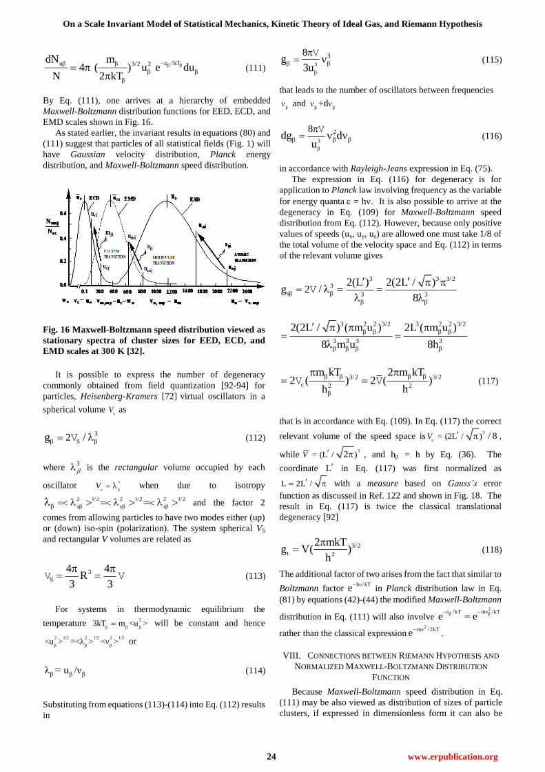
On a Scale Invariant Model of Statistical Mechanics, Kinetic Theory of Ideal Gas, and Riemann Hypothesis
24 www.erpublication.org
/kTu 3/2 2dN m
4 ( ) u e duN 2 kT
(111)
By Eq. (111), one arrives at a hierarchy of embedded
Maxwell-Boltzmann distribution functions for EED, ECD, and
EMD scales shown in Fig. 16.
As stated earlier, the invariant results in equations (80) and
(111) suggest that particles of all statistical fields (Fig. 1) will
have Gaussian velocity distribution, Planck energy
distribution, and Maxwell-Boltzmann speed distribution.
Fig. 16 Maxwell-Boltzmann speed distribution viewed as
stationary spectra of cluster sizes for EED, ECD, and
EMD scales at 300 K [32].
It is possible to express the number of degeneracy
commonly obtained from field quantization [92-94] for
particles, Heisenberg-Kramers [72] virtual oscillators in a
spherical volume S
V as
3
S2g / V (112)
where 3
is the rectangular volume occupied by each
oscillator 3
oV
when due to isotropy
2 1/2 2 1/2 2 1/2
x y z and the factor 2
comes from allowing particles to have two modes either (up)
or (down) iso-spin (polarization). The system spherical VS
and rectangular V volumes are related as
3
S
4 4R
3 3
V V (113)
For systems in thermodynamic equilibrium the
temperature 2
β β β3kT m <u > will be constant and hence
2 1/2 2 1/2 2 1/2
β β β<u > <λ > <ν >= or
β β βλ u /ν= (114)
Substituting from equations (113)-(114) into Eq. (112) results
in
3
38g
3u
V (115)
that leads to the number of oscillators between frequencies
βν and
β βν ν+d
3
28dg d
u
V (116)
in accordance with Rayleigh-Jeans expression in Eq. (75).
The expression in Eq. (116) for degeneracy is for
application to Planck law involving frequency as the variable
for energy quanta = h. It is also possible to arrive at the
degeneracy in Eq. (109) for Maxwell-Boltzmann speed
distribution from Eq. (112). However, because only positive
values of speeds (ux, uy, uz) are allowed one must take 1/8 of
the total volume of the velocity space and Eq. (112) in terms
of the relevant volume gives
3 3 3/2
3
s 3 32
2(L ) 2(2L / )g /
8
V
3 2 2 3/2 3 2 2 3/2
3 3 3 3
2(2L / ) ( m u ) 2L ( m u )
8 m u 8h
3/2 3/2
c 2 2
m kT 2 m kT2 ( ) 2 ( )
h h
V V (117)
that is in accordance with Eq. (109). In Eq. (117) the correct
relevant volume of the speed space is3
c= (2L / ) / 8V ,
while3
= (L / )2V , and h = h by Eq. (36). The
coordinate L in Eq. (117) was first normalized as
L 2L / with a measure based on Gauss’s error
function as discussed in Ref. 122 and shown in Fig. 18. The
result in Eq. (117) is twice the classical translational
degeneracy [92]
3/2
t 2
2 mkTg V( )
h
(118)
The additional factor of two arises from the fact that similar to
Boltzmann factor h /kT
e
in Planck distribution law in Eq.
(81) by equations (42)-(44) the modified Maxwell-Boltzmann
distribution in Eq. (111) will also involve 2
/kT mv /kTe e
rather than the classical expression2
mv /2kTe
.
VIII. CONNECTIONS BETWEEN RIEMANN HYPOTHESIS AND
NORMALIZED MAXWELL-BOLTZMANN DISTRIBUTION
FUNCTION
Because Maxwell-Boltzmann speed distribution in Eq.
(111) may be also viewed as distribution of sizes of particle
clusters, if expressed in dimensionless form it can also be
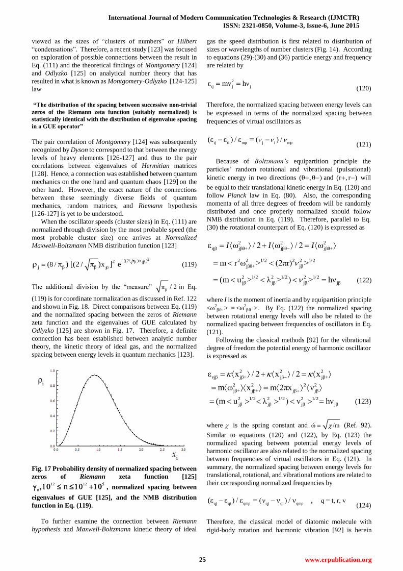
International Journal of Modern Communication Technologies & Research (IJMCTR)
ISSN: 2321-0850, Volume-3, Issue-6, June 2015
25 www.erpublication.org
viewed as the sizes of ―clusters of numbers‖ or Hilbert
―condensations‖. Therefore, a recent study [123] was focused
on exploration of possible connections between the result in
Eq. (111) and the theoretical findings of Montgomery [124]
and Odlyzko [125] on analytical number theory that has
resulted in what is known as Montgomery-Odlyzko [124-125]
law
“The distribution of the spacing between successive non-trivial
zeros of the Riemann zeta function (suitably normalized) is
statistically identical with the distribution of eigenvalue spacing
in a GUE operator”
The pair correlation of Montgomery [124] was subsequently
recognized by Dyson to correspond to that between the energy
levels of heavy elements [126-127] and thus to the pair
correlations between eigenvalues of Hermitian matrices
[128]. Hence, a connection was established between quantum
mechanics on the one hand and quantum chaos [129] on the
other hand. However, the exact nature of the connections
between these seemingly diverse fields of quantum
mechanics, random matrices, and Riemann hypothesis
[126-127] is yet to be understood.
When the oscillator speeds (cluster sizes) in Eq. (111) are
normalized through division by the most probable speed (the
most probable cluster size) one arrives at Normalized
Maxwell-Boltzmann NMB distribution function [123]
j
2[(2/ ) ]j2
j
x8 / x( ) (2 / ) e[ ]
(119)
The additional division by the ―measure‖ β
π 2/ in Eq.
(119) is for coordinate normalization as discussed in Ref. 122
and shown in Fig. 18. Direct comparisons between Eq. (119)
and the normalized spacing between the zeros of Riemann
zeta function and the eigenvalues of GUE calculated by
Odlyzko [125] are shown in Fig. 17. Therefore, a definite
connection has been established between analytic number
theory, the kinetic theory of ideal gas, and the normalized
spacing between energy levels in quantum mechanics [123].
Fig. 17 Probability density of normalized spacing between
zeros of Riemann zeta function [125] 12 12
nn
, normalized spacing between
eigenvalues of GUE [125], and the NMB distribution
function in Eq. (119).
To further examine the connection between Riemann
hypothesis and Maxwell-Boltzmann kinetic theory of ideal
gas the speed distribution is first related to distribution of
sizes or wavelengths of number clusters (Fig. 14). According
to equations (29)-(30) and (36) particle energy and frequency
are related by
2
tj j jνε mv h
(120)
Therefore, the normalized spacing between energy levels can
be expressed in terms of the normalized spacing between
frequencies of virtual oscillators as
tj ti mp j i mp(ε ε ) / ε = ( ) /
(121)
Because of Boltzmann’s equipartition principle the
particles‘ random rotational and vibrational (pulsational)
kinetic energy in two directions (θ ,θ ) and (r , r ) will
be equal to their translational kinetic energy in Eq. (120) and
follow Planck law in Eq. (80). Also, the corresponding
momenta of all three degrees of freedom will be randomly
distributed and once properly normalized should follow
NMB distribution in Eq. (119). Therefore, parallel to Eq.
(30) the rotational counterpart of Eq. (120) is expressed as
2 2 2
rjβ jβθ+ jβθ jβθ+ε ω / 2 ω / 2 ωI I I
2 2 1/2 2 2 1/2
jβθ+ jβm r ω > (2πr) >
2 1/2 2 1/2 2 1/2
jβ jβ jβ jβ(m u > λ > ) > hν (122)
where I is the moment of inertia and by equipartition principle
<2> =<
2>. By Eq. (122) the normalized spacing
between rotational energy levels will also be related to the
normalized spacing between frequencies of oscillators in Eq.
(121).
Following the classical methods [92] for the vibrational
degree of freedom the potential energy of harmonic oscillator
is expressed as
2 2 2
vjβ jβ+ jβ jβ+ε x / 2 x / 2 x
2 2 2 2
jβ+ jβ+ jβ jβm ω x m 2πx ν
2 1/2 2 1/2 2 1/2
jβ jβ jβ jβ(m u λ ) ν hν (123)
where is the spring constant and ω /m (Ref. 92).
Similar to equations (120) and (122), by Eq. (123) the
normalized spacing between potential energy levels of
harmonic oscillator are also related to the normalized spacing
between frequencies of virtual oscillators in Eq. (121). In
summary, the normalized spacing between energy levels for
translational, rotational, and vibrational motions are related to
their corresponding normalized frequencies by
qj qi qmp qj qi qmpν q = t, r, v(ε ε ) / ε = ( ν ) / ν ,
(124)
Therefore, the classical model of diatomic molecule with
rigid-body rotation and harmonic vibration [92] is herein

On a Scale Invariant Model of Statistical Mechanics, Kinetic Theory of Ideal Gas, and Riemann Hypothesis
26 www.erpublication.org
considered to also possess an internal translational harmonic
motion. The internal translational degree of freedom is
associated with thermodynamic pressure and may therefore
be called internal potential energy. In addition to this internal
harmonic translation there will be an external harmonic
motion due to the peculiar translational velocity in Eq. (3) and
a corresponding external potential energy (Fig. 15). In Sec.
11, it will be shown that the external potential energy appears
in Schrödinger equation (206) and acts as Poincaré stress
[117-119] that is responsible for ―particle‖ stability. The
particle trajectory under all four degrees of freedom namely
the three internal translational, rotational and vibrational
motions and the external peculiar motion will be quite
complicated. Clearly, addition of radial oscillations about the
center of mass to the rigid rotator will result in particle motion
on a radial wave, de Broglie wave, along the circumference of
the otherwise circular particle trajectory.
Now that the normalized spacing between energy levels
have been related to the normalized spacing between
oscillator frequencies j in Eq. (124), the latter should be
connected to the zeros of Riemann zeta function. The zeros
of Riemann zeta function are related to prime numbers
through Euler‘s Golden Key [126]
j
s 1
js
1ζ(s) (1 )
n p
pn
(125)
where s = a +ib is a complex number. Clearly, the zeros of
zeta function in Eq. (125) will coincide with the zeros of the
powers of primes
s a ib
j j0p p
(126)
It is most interesting that according to his Nachlass [127]
Riemann was working on the problem of Riemann
Hypothesis and the hydrodynamic problem of stability of
rotating liquid droplets simultaneously. In view of Eq. (119)
and the connections between normalized energy and
frequency spacing shown in Fig. 17, it is natural to consider
the situation when particle frequencies are given by integral
powers of prime numbers as
j
1 2 3
j j j j j, , ...
N
pp p p p
(127)
in harmony with Gauss’s clock calculator [127] and Hensel’s
pj-adic numbers j
p (Ref. 126).
Now, since the atomic energy of particles must be
quantized according to Planck formula ε h by Eq. (127)
one writes
j
2
j j jmv = h h h
N
pp
(128)
that by equations (30)-(31) and (36) suggest that the particle
velocity may be expressed as
N/2+iNblnN/2 1/2+ ib
j j j
iθh/m h/m h/mj
j
p
pp e p
v
(129)
where the angle j
Nb lnθ p corresponds to the direction of
velocity vector. Therefore, by Eq. (129) the particle energy
consistent with Eq. (128) becomes
j
* N
j j j jε = m( . ) h h
pp v v
(130)
Also, the dependence of particle speed on j
pwill be
obtained from equations (128) and (129) as
j
N/2 1/2
j jv h/m h/m
pp
(131)
that by the relation j j j
v = λ gives particle wavelength
j
1/2
jλ h/m
p
(132)
In the following it is shown that with the value a = ½ as the
position of the critical line in accordance with Riemann
Hypothesis [126, 127] the zeros of particle velocities from
Eq. (129) will coincide with the zeros of Riemann zeta
function in Eq. (126). One also expects the zeros of particle
velocity from Eq. (129) to coincide with the zeros of particle
speed in Eq. (131), and those of particle energy and hence
frequency in Eq. (128). Thus, at thermodynamic equilibrium
all points of the normalized Maxwell-Boltzmann distribution
in Fig. 17 correspond to stochastically stationary states of
clusters of particles undergoing random translational,
rotational, vibrational motions while satisfying the principle
of detailed balance of quantum mechanics through
continuous transitions between clusters (energy levels)
further discussed in Sec. 11.
At thermodynamic equilibrium Maxwell-Boltzmann
speed distribution in Eq. (119) corresponds to translational,
rotational, and vibrational particle velocities that must follow
Gaussian distribution like Fig. 5. Also, space isotropy
requires that the translational, rotational, and vibrational
momenta of particles in two directions+
( , )x x
, +
(θ θ, )
,
+(r r, )
be equal in magnitude and opposite in direction such
that by Eq. (129) at the zeros of particle velocity
b
jln ( )1/2
j
1/N 2N
j h/mi p
p e
v
1/2 b b
j j j
2N [cos(ln ) sin(ln )] 0h/mp p i p (133a)
the corresponding particle momenta become identically zero.
Therefore, one expects ―stationary states‖ at mean
translational position ( 0)x , mean angular
position (θ 0) , and mean radial position ( r 0) at which
particle velocities t θ v
(v , v , v ) and hence energies
t θ v(ε , ε , ε ) vanish. Hence, another argument for the position
of the critical line being at a = ½ could be based on symmetry
requirements for passage across stationary states and the
Gaussian velocity distribution (Fig. 5) at equilibrium.
Because by Eq. (124) all three forms of energy could be
expressed as products of Planck constant and frequency, one
identifies the zeros of velocities in Eq. (129) as the

International Journal of Modern Communication Technologies & Research (IJMCTR)
ISSN: 2321-0850, Volume-3, Issue-6, June 2015
27 www.erpublication.org
―stationary states‖ of particle‘s translational, rotational, and
vibrational momenta. The connection between the kinetic
theory of ideal gas and Montgomery-Odlyzko law shown in
Fig. 17 involves spacing between particle speeds in Eq. (131)
whereas the zeros of Riemann zeta function are related to
stationary states or the zeros of particle velocities in Eq.
(129). However, the zeroes of particle speeds must coincide
with the zeros of particle velocities that from Eq. (133a) are
given by
1/2 ib
j0p
(133b)
Comparison between the zeros of particle velocity at
stationary states in Eq. (133b) and the zeros of Riemann zeta
function in Eq. (126) shows that they will coincide if a = ½
namely on the critical line in accordance with Riemann
hypothesis.
It is interesting to examine the connection between
analytical number theory and Riemann hypothesis in terms of
particle wavelengths in Eq. (132) hence quantized spatial
coordinates rather than particle speeds in Eq. (131). In a
recent study [122] a logarithmic system of coordinates was
introduced as
Ax ln N (134)
whereby the spatial distance of each statistical field (Fig. 1) is
measured on the basis of the number of ―atoms‖ of that
particular statistical field NA. With definition in Eq. (134)
the counting of numbers must begin with the number zero
naturally since it corresponds to a single atom. The number of
atoms in the system is expressed as [122]
ESN
AS AEN N
(135)
where AS ES AE
(N , N N ),
respectively refer to the number of
atoms in the system, number of elements in the system, and
number of atoms in the element. The hierarchy of the resulting
normalized coordinates is shown below [122]
. . .
L _________________1 ______ 0
1L ___ 11 10
. . . (136)
The exact connections between spatial coordinates of
hierarchies of statistical fields (Fig. 1) will involve the
important concept of re-normalization [130,131].
Normalization in Eq. (136) is based on the concept of
―dimensionless‖ or ―measureless‖ numbers [122]
ESx x / N (137)
where the ―measure‖ is defined by Gauss’s error function
as
21 1
1
x
1 10
e dx / 2
(138)
In view of equations (137)-(138), the range ( 1 ,1 )
of the
outer coordinate x will correspond to the range 1 1
( , )
of the inner coordinate 1x leading to the coordinate
hierarchy schematically shown in Fig. 18.
+ 1 1 + 1 0 + 1 1 +1
0 1 1
+1
= 2
= 2
Fig. 18 Hierarchy of normalized coordinates associated
with embedded statistical fields [122].
As discussed above and in [123] one naturally considers
the prime numbers p1 = 2, p2 = 3, p3 = 5, …, to be the
―atoms‖ of the statistical field at scale that may also be
viewed as different atomic ―species‖. However in view of
equations (127) and (132) space quantization will be based on
the inverse power of pj-adic numbers such that by Eq. (135)
ESj ESjN /2 N /21/2
ASj AEj jN N p
(139)
that parallel to Eq. (132) is expressed as
ESjN /2 1/2
j j m jh / m h / m
pp
(140)
The reason for the choice of primes is that they represent
indivisible ―atoms‖ of arithmetic out of which all natural
numbers at any scale could be constructed. The quantized
wavelengths in Eq. (140) like Eq. (132) will correspond to
quantized frequencies in Eq. (127), energies in Eq. (130), and
speeds in Eq. (131) all involving pj-adic numbers jβ
pthat
were employed in the construction of Adele space of
noncommutative spectral geometry of Connes [126, 127,
132].
The wavelength in Eq. (140) is next normalized with
respect to the most probable cluster size
N/2 1/2
mj j m jh / m h / m
pp
(141)
and since at thermodynamic equilibrium the entire
distribution function (Fig. 17) is stochastically stationary at

On a Scale Invariant Model of Statistical Mechanics, Kinetic Theory of Ideal Gas, and Riemann Hypothesis
28 www.erpublication.org
all particle speeds j j j
v cons tan t
equations (102),
(103), (140), and (141) give
j
mp j j
j j jm
1/2N /2
pj1
j 1/2N/2
mpj
vx
v
p
p
(142)
With pj-adic numbers jβ
pincorporated into the quantized
wavelengths in Eq. (142) one arrives at dimensionless speeds
in Eq. (131) and hence the Normalized Maxwell-Boltzmann
(NMB) distribution in Eq. (119) for the prime ―specie‖ pj.
To summarize, first the normalized spacing between
energy levels were related to the normalized spacing between
oscillator frequencies in Eq. (124). Next, oscillator
frequencies were taken as pj-adic numbers in Eq. (127) and
the spacing between frequencies and zeros of energy levels in
Eq. (128) were related to the spacing between ―stationary
states‖ or zeros of particle velocity in Eq. (129), that were in
turn related to the zeros of Riemann zeta function by Eq.
(126) through Euler’s golden key in Eq. (125). The model
therefore provides a physical explanation of
Montgomery-Odlyzko [126, 127]
law as well as
Hilbert-Polya [126] conjecture that spacing between the
zeros of Riemann zeta function are related to spacing between
eigenvalues of Hermitiam matrices. The close agreement
shown in Fig. 17 is because at equilibrium by Eq. (124) the
distribution of normalized particle energy in Eq. (130) and
speed in Eq. (131) are related by Maxwell-Boltzmann
distribution in Eq. (119). Moreover, because particle energy
vanishes at the stationary states given by Eq. (133b) the
energy spectrum will correspond to absorption spectrum in
accordance with the prediction of noncommutative spectral
geometry of Connes [132]. For complete resolution of
Riemann Hypothesis one must now identify the appropriate
normalization method to relate the zeros of Riemann zeta
function by Eq. (125) hence Eq. (126) to the zeros of particle
velocity in Eq. (129) hence Eq. (133b) that is simpler than the
Riemann-Siegel formula [126].
Since each partial density in Eq. (119) corresponds to
single ―prime‖ specie, one next constructs a mixture density
by summing all the partial probability densities of all ―prime‖
species
j
j
ρ ρ (143)
to arrive at
2[(2/ ) ]2 x8 / x( ) (2 / ) eρ [ ]
(144)
where
22
jj2 2
j j2 2
m m
j
j2
m
m vvx v
v mv
1Y
v
.
2
2
2
m
vx
v
(145)
because the mean energy of all species are identical at
thermodynamic equilibrium2 2
mj mij im v m v kT . The
grand ensemble of NMB pj-adic statistical fields in Eq. (144)
will have a corresponding GUE that could be identified as
Connes [124-127, 132] Adele space Aat a particular
scale. Therefore, the normalized Adele space Aat any
particular scale is constructed from superposition of
infinite NMB distribution functions like Fig. 17
corresponding to atomic specie pj and cluster sizes in the
form of pj-adic numbers.
With prime numbers pj as atomic species the spacing
between wavelengths of number clusters or Hilbert
condensations [126] are related to the spacing between
particle speeds by Eq. (142) that are in turn related to the
normalized spacing between energy levels by Eq. (124). The
connection to quantum mechanics is further evidenced by
direct derivation of Maxwell-Boltzmann speed distribution in
Eq. (111) from Planck distribution in Eq. (80) discussed in
Sec. 7. Also, because the GUE associated with Eq. (144) is
based on pj-adic type numbers, the normalized spacing
between its eigenvalues should be related to the normalized
spacing between the zeros of Riemann zeta function
according to the theory of noncommutative geometry of
Connes [132]. Although the exact connection between
noncommutative geometry and Riemann hypothesis is yet to
be understood according to Connes [127]
“The process of verification can be very painful: one’s
terribly afraid of being wrong…it involves the most
anxiety, for one never knows if one’s intuition is right- a
bit as in dreams, where intuition very often proves
mistaken”
the model suggested above may help in the clarification of the
physical foundation of such a mathematical theory.
The scale invariance of the model, possible
electromagnetic nature of all matter discussed in Sec. VI, as
well as the connection between analytic number theory and
the kinetic theory of ideal gas (Fig. 17) all appear to confirm
the perceptions of Sommerfeld [133]
"Our spectral series, dominated as they are by integral
quantum numbers, correspond, in a sense, to the ancient
triad of the lyre, from which the Pythagoreans 2500 years
ago inferred the harmony of the natural phenomena; and
our quanta remind us of the role which the Pythagorean
doctrine seems to have ascribed to the integers, not merely
as attributes, but as the real essence of physical
phenomena."
as well as those of Weyl [134].
Since the physical space or Casimir [73] vacuum itself is
identified as a fluid and described by a statistical field [34,
83], it will have a spectrum of energy levels given by
Schrödinger equation (206) that in view of Heisenberg [135,
34, 83] matrix mechanics will be described by
noncommutative spectral geometry of Connes [132]. Hence,
the above results in harmony with the perceptions of
Pythagoras and Plato suggest that pure ―numbers‖ maybe the
basis of all that is physically ―real‖ [34, 136].

International Journal of Modern Communication Technologies & Research (IJMCTR)
ISSN: 2321-0850, Volume-3, Issue-6, June 2015
29 www.erpublication.org
IX. INVARIANT TRANSPORT COEFFICIENTS AND
HIERARCHIES OF ABSOLUTE ZERO TEMPERATURES AND
VACUA
Following Maxwell [36, 39] the scale invariant definition
of kinematic viscosity β β β
/ may be expressed as
β β β β 1 β 1
1 1u v
3 3λ
(146)
At the scale of = e corresponding to equilibrium eddy
dynamics EED (Fig. 1) equation (146) gives Boussinesq eddy
diffusivity [137]
e e e c c
1 1u v
3 3λ
(147)
On the other hand, the kinematic viscosity at LCD scale
involves the ―atomic‖ length cor the molecular mean free
path m that appears in Maxwell’s formula for kinematic
viscosity [30]
c c c m m
1 1u λ v
3 3 (148)
associated with viscous dissipation in fluid mechanics. It is
important to note that the model predicts a finite kinematic
viscosity for the scale = s i.e. electrodynamics scale when
energy can be dissipated to Casimir [73] vacuum at the lower
chromodynamics scale
k k ks s s k k
k
λ v m1 1 1u λ v
3 3(2π) 3(2π) m
k
k k
h1
3(2π) m 3m (149)
in exact agreement with the result of de Broglie [3] provided
that the equality of particle mean free path and
wavelengthk k
λλ holds. Therefore, Ohmic dissipation could
occur by transfer of energy from electrons into photon gas
constituting Casimir [73] vacuum. In view of Fig. 1, it is
natural to expect that energy of photon field at
chromodynamics scale could be dissipated into a
sub-photonic tachyon field that constitutes a new vacuum
called vacuum-vacuum. According to the model
electromagnetic waves propagate as viscous flow due to
―viscosity‖ of radiation [41] or gravitational viscosity [138]
in harmony with the well-known concept of ―tired light‖.
In view of the definition of Boltzmann constant in
equations (30b), (33) and (36), Kelvin absolute temperature is
related to the most probable wavelength of oscillations by Eq.
(90) and hence becomes a length scale. Therefore, Kelvin
absolute temperature approaches zero through an infinite
hierarchy of limits as suggested by Eq. (136) and Fig. 18. In
other words, one arrives at a hierarchy of ―absolute zero‖
temperatures defined as
. . .
β β β 1 β 1
T 0 T 1
β-1 β-1 β-2 β-2T 0 T 1
. . . (150)
As discussed in Sec.VI, physical space could be identified
as a tachyonic fluid [139] that is the stochastic ether of Dirac
[111] or "hidden thermostat" of de Broglie [3]. The
importance of Aristotle’s ether to the theory of electrons was
emphasized by Lorentz [140-141]
"I cannot but regard the ether, which is the seat of an
electromagnetic field with its energy and its vibrations,
as endowed with certain degree of substantiality,
however different it may be from all ordinary matter"
Also, in Sec. 6 photons were suggested to be composed of a
large number of much smaller particles [139], like neutrinos
that themselves are composed of large numbers of tachyons
[107]. Therefore, following Casimir [73] and in harmony with
Eq. (150) one expects a hierarchy of vacua
β β-1(vacuum-vacuum) ( acuum)v
(151)
as one attempts to resolve the granular structure of physical
space and time at ever smaller scales described by the
coordinates in Eq. (136).
The hierarchies of coordinates in Eq. (136) and vacua in
Eq. (151) will have an impact on the important recurrence
theory of Poincaré [44] and its implication to Boltzmann’s
expression of thermodynamic entropy
k lnS W (152)
In particular, the conflict between Poincaré recurrence theory
and thermodynamic irreversibility emphasized by Zermelo
[142] should be reexamined. As was emphasized by
Boltzmann [143] Poincaré [44] recurrence theory cannot be
applied to thermodynamic systems because such systems
cannot be truly isolated. That is, the unattainable nature of
absolute vacuum-vacuum in Eq. (151) makes isolation of all
physical systems impossible. The same limitation will apply
to the entire universe when our universe is considered to be
just one universe as an open system among others according
to Everett’s many universe theory described by DeWitt [144].
The hierarchy of vacua in Eq. (151) is in harmony with the
inflationary theories of cosmology [145-148] and the finite
pressure of Casimir [73] vacuum given by the modified van
der Waals law of corresponding states [149]
r
r c2
c r r
T1 9 3p Z
Z v 1/ 3 8v 8
(153)
where Zc is the critical compressibility factor.
Clearly, the nature of thermodynamic irreversibility will
be impacted by both the hierarchical definition of time
discussed in [34] as well as the cascade of embedded

On a Scale Invariant Model of Statistical Mechanics, Kinetic Theory of Ideal Gas, and Riemann Hypothesis
30 www.erpublication.org
statistical fields shown in Fig. 1. For example, let us consider
at EED scale a hydrodynamic system composed of 2
10 fluid
elements each of which composed of 2
10 clusters of eddies.
Next, let eddy, defined as the most probable size ensemble of
molecular-clusters at ECD scale, be composed of 2
10 mean
molecular-clusters each containing 8
10 molecules. Let us
next assume that only the cluster i of the eddy j of the fluid
element f contains molecules of type B and that all other
clusters of all other eddies are composed of molecules of type
A. The system is then allowed to fully mix at the molecular
level. The thermodynamic reversibility will now require that 8
10 type B molecules to first become unmixed at
hydrodynamic scale by leaving (2
10 -1) fluid elements and
collecting in the fluid element f. Next, all 8
10 type B
molecules must leave (2
10 -1) eddies and collect in the eddy
ejf. Finally 8
10 type B molecules must leave (2
10 -1) clusters
of eddy j and collect in the cluster cijf. Clearly the probability
of such preferential motions to lead to immixing against all
possible random motions will be exceedingly small. When
the above hierarchy of mixing process is extended to yet
smaller scales of molecular-dynamics, electrodynamics, and
chromo-dynamics, the probability for reversibility becomes
almost zero bordering impossibility in harmony with
perceptions of Boltzmann [38]. The broader implications of
the hierarchy of coordinate limits in Eq. (136) to the internal
set theory of Nelson [150] and the recurrence theory of
Poincaré [44] require further future investigations.
X. INVARIANT FORMS OF THE FIRST LAW OF
THERMODYNAMICS AND DEFINITION OF ENTROPY
In this section, Boltzmann statistical mechanics for ideal
monatomic gas discussed in Sec. 7 will be applied to arrive at
invariant forms of Boltzmann equation for entropy and the
first law of thermodynamics. The results also suggest a new
perspective of the nature of entropy by relating it to more
fundamental microscopic parameters of the thermodynamic
system.
As stated in Sec. 3, when the three velocities m m m
( , , )Vu v
in Eq. (3) are all random the system is composed of an
ensemble of molecular clusters and single molecules under
equilibrium state and one obtains from Eq. (3)
2 2 2
x x xm m m
u v V
t tke pe tkeˆ ˆ ˆ ˆ ˆpv
(154)
as the sum of the internal translational kinetic and ―external‖
potential energies sincex x
2 0
v V . One next allows the
monatomic particles to also possess both rotational rke
and
vibrational (pulsational) vke kinetic energy [31] and invokes
Boltzmann‘s principle of equipartition of energy such that
2
t x tke rke vke peˆ ˆ ˆ ˆm
v
(155)
With the results in Eqs. (154)-(155) the total energy of the
particle could be expressed as [32]
ˆ ˆ ˆh pu v (156)
where h
is the enthalpy, vis the volume and
tke rke ke tkeˆ ˆ ˆ ˆˆ 3u
(157)
is the internal energy per molecule such that by Eq. (156)
pH U V
(158)
where N ˆV v , N hH
, and N ˆU u
are
respectively volume, enthalpy, and internal energy.
In accordance with the perceptions of Helmholtz, one may
view Eq. (158) as the first law of thermodynamics
Q U W
(159)
when reversible heat and work are defined as [31]
TQ H S
(160)
and
pW V
(161)
and S is the entropy. For an ideal gas equations (159) and
(160) lead to
T p HQ S U =V
3N kT N kT 4N kT+ =
(162)
When photons are considered as monatomic ideal gas
integration of Eq. (81) and maximization of Eq. (58) are
known to lead to internal energy and entropy [92-94]
4 5 4 3
3 3
8 kT) 32 k T
) )
( ,
15(hc 45(hc
V VU S
(163)
Since Poisson coefficient of photon is p v
ˆ ˆc c 4 / 3/ the
result in Eq. (162) leads to
T4
3S U
(164)
in accordance with Eq. (163). Also, since for an ideal gas
equations (157) and (159) give
tke3 3p 3N kTU V
(165)
by Eq. (162) entropy per photon k
ˆ / Ns S becomes [32]

International Journal of Modern Communication Technologies & Research (IJMCTR)
ISSN: 2321-0850, Volume-3, Issue-6, June 2015
31 www.erpublication.org
kˆ 4ks
(166)
as compared to
kˆ 3.6ks
(167)
based on the classical model [94].
The discrepancy between equations (166) and (167) is due
to the classical formulation [94] for the number of photons in
a given volumeV. It is possible to express the total potential
energy from the integration of mean energy and number
density of oscillators over for spherical number density space
as
N N
0 0dN kTdN NkT
2N N
2 xx h /kT0 0
h (8 N )n (4 N )dN dN
e 1
2N
h /kT0
h (8 N / 3)dN
e 1
(168)
One next considers the relation between the number of
quantized oscillators in a cube of size L = Lx = Ly = Lz as
xN L / L / c
(169)
and the isotropy condition
2 2 2 2 2
x y z xN N N N 3N
(170)
Because de Broglie [2]
―matter wave packets‖ or
Heisenberg-Kramers [72]
virtual oscillators are now
considered to represent actual particles of ideal gas according
to Eq. (169) one requires integral numbers N of the full
wavelength , as opposed to the conventional half
wavelength 2 to fit within the cavity of length L.
Substituting from equations (169)-(170) into Eq. (168) gives
2 2
h /kT0
8 h (L / c)NkT (L / c)d
3 e 1
=
3 3
3 h /kT0
8 hLd
3c e 1
4 3
3 x0
kT)
)
8 ( xdx
3 (hc e 1
V
5 4
3
kT)
)
8 (
45 (hc
V (171)
Hence, the number of photons in volume V is given by Eq.
(171) as
35
kT8N
45 hc
V
(172)
as compared to the classical result [94]
3
kTN 8 2.404
hcV (173)
Also, from equations (172) and (162) one obtains the internal
energy [32]
3NkTU (174)
that leads to the expected specific heat at constant volume
o
vc 3R (175)
that is in accordance with Eq. (106)
The result in Eq. (174) only approximately agrees with the
classical expression for the internal energy [93-94]
4
NkT
30 (3)U
(176)
that leads to
2.701NkTU (177)
According to Eq. (171) the expression in Eq. (176) should
involve zeta function of 4 rather than 3 such that
4
NkT3NkT
30 (4)U
(178)
that agrees with Eq. (174) and by Eq. (162) leads to the ideal
gas law [32]
p NkTV
(179)
instead of the classical result [93]
p 0.900NkTV (180)
for equilibrium radiation.
Concerning the results in equations (177) and (180) it
was stated by Yourgrau et al. [93]
“The reader will not fail to recognize the close
resemblance between relations and their counterparts
pertaining to a classical ideal gas”
With the modified results in equations (174) and (179) the
correspondence between photon gas and classical ideal gas
becomes exact thus closing the gap between radiation and gas
theory discussed by Darrigol [151] and Stachel [152]. The
important relation between radiation pressure and internal
energy [92-94]

On a Scale Invariant Model of Statistical Mechanics, Kinetic Theory of Ideal Gas, and Riemann Hypothesis
32 www.erpublication.org
ˆ ˆp / 3 / 3 / 3U V u v u (181)
is exactly satisfied by equations (174) and (179) and closely
but only approximately satisfied by equations (173) and
(180).
Since Kelvin absolute temperature scale is identified as a
length scale by Eq. (90), thermodynamic temperature relates
to spatial and hence temporal ―measures‖ of the physical
space [34] or Casimir [73] vacuum. Therefore, the hierarchy
of limiting zero temperatures in Eq. (150) will be related to
hierarchy of ―measures‖ that are employed to renormalize
[130, 131] ―numbers‖ by equations (137)-(138) and arrive at
―dimensionless‖ coordinates (Fig. 18) as discussed earlier
[122]. For an ideal monatomic gas one has the o
pc 4R and
o
vc 3R such that Eq. (162) reduces to the identity
4 3 1
(182)
Therefore, the mathematical relation (182) always holds for
statistical fields of any scale (Fig. 1) as the thermodynamic
temperature in Eq. (150) approaches the ―absolute zero‖
0T (
1 11T
) associated with coordinates of that
particular scale in Eq. (136).
The result in Eq. (162) could be also obtained from the
Gibbs equation
j j
j
ˆT d p dNdS U dV
(183)
, Gibbs-Duhem equation
j j
j
ˆdT dp N dS V (184)
and the equality of molar Gibbs free energy and chemical
potential j j
ˆ ˆg of j specie. Addition of equations (183) and
(184) leads to Euler equation
j j
j
ˆd(T ) d d(p ) d NS U V g
d d(p ) dU V G (185)
At the state of thermodynamic equilibrium dG = 0 equation
(185) leads to Eq. (162) upon integration and application of
Nernst-Planck third law of thermodynamics requiring
βh 0 in the limit β
T 0 (Ref. 31).
Next, the invariant Boltzmann equation (152) for entropy
is introduced as
j jk ln WS
(186)
Hence
jβ j j
j j j
k ln W k ln WS
(187)
or
β k ln WS (188)
Substituting in Eq. (186) from Eq. (60) and applying
Stirling’s formula gives
jN
j j j jk ln W k ln(g / N !)S
j j j j jk[N ln g N ln N N )
j j jkN [ln(g / N ) 1] (189)
Also, substituting for Boltzmann distribution from Eq. (67)
into Eq. (189) leads to
j j j jˆkN [ / kT / kT 1]S
(190)
or
j j j j j jˆT N N kT NS
j j j j j j
ˆp NU V g H G (191)
Since Gibbs free energy is by definition
j j jTG H S
(192)
one obtains from equations (191) and (185)
1 (193)
The results in equations (191) and (193) lead to Euler
equation
j j j jT pS U V G
(194)
Summation of Eq. (194) over all energy levels results in
T pS U V G
(195)
Since the principle of equipartition of energy of
Boltzmann by equations (155) and (162) leads to [32]
j j j j j j jtkeT 4N k T 4NH Q S
(196)
in view of Eq. (30b) the definition of entropy is introduced as
Boltzmann factor 2 1/2 2 1/2
j j j j ˆ 4k 4m us (197)
that by Eq. (36) when multiplied by ―temperature‖ 2 1/ 2
jjT
gives the ―atomic‖ enthalpy of the energy level j
at equilibrium [32]
j j j j j j jˆ ˆ ˆh 4k T 4kT T Ts s
(198)
At EKD scale = k, the results in equations (196)-(198) are
in accordance with Eq. (166) for photon gas. Also, Eq. (198)

International Journal of Modern Communication Technologies & Research (IJMCTR)
ISSN: 2321-0850, Volume-3, Issue-6, June 2015
33 www.erpublication.org
is parallel to the way the universal Boltzmann constant k
times equilibrium temperature T relates to the most probable
atomic internal energy
2
mp mpˆ 3kT m uu
(199)
At thermodynamic equilibrium the temperatures of all energy
levels are identical j
T T such that both Planck energy
spectrum (Fig. 6) and Maxwell-Boltzmann speed spectrum
(Fig. 16) correspond to an isothermal statistical field at a
given thermodynamic temperature T. Hence, in Eq. (199)
the most probable atomic internal energy is given as the
product of temperature and the universal Boltzmann constant
k from Eq. (36). In Eq. (198) the atomic enthalpy is given as
product of temperature and atomic entropy defined in Eq.
(197) for the energy level j.
The invariant first law of thermodynamics in Eq. (162)
when expressed per molecule, per unit mole, and per unit
mass appears as [32]
ˆ ˆˆ ˆ ˆ ˆh u RT u kT u p v (200a)
oh u RT u R T u p v (200b)
j j j j j j jh u R T u R T u p v
(200c)
Thus one may express the universal gas constant per
molecule, per mole, and per unit mass j
ˆ(R, R, R ) as
o oR R / N k (201a)
o oR = R = kN (201b)
o o o
j j j jR R R/ W / (N m ) k / m (201c)
XI. INVARIANT SCHRODINGER AND DIRAC WAVE
EQUATIONS
The fact that the energy spectrum of equilibrium isotropic
turbulence is given by Planck distribution (Figs. 6-10) is a
strong evidence for quantum mechanical foundation of
turbulence, [33, 34]. This is further supported by derivation
of invariant Schrödinger equation from invariant Bernoulli
equation in [34]. Hydrodynamic foundation of Schrödinger
equation suggests that Bohr stationary states in quantum
mechanics are connected to stationary sizes of clusters, de
Broglie wave packets, in equilibrium fields. When both
vorticity and iso-spin defined in Eq. (13) are zero one has a
Hamiltonian non-dissipative system and for non-reactive
incompressible fluid the flow field will be potential with
v and the continuity Eq. (5) and Cauchy equation
of motion (7) lead to invariant Bernoulli equation [34]
2
( ) [ ( )]p cons tan t 0
t 2
(202)
The constant in Eq. (202) is set to zero since pressure acts as a
potential that is only defined to within an additive constant.
Comparison of Eq. (202) with Hamilton-Jacobi equation of
classical mechanics [2] written in invariant form
2
S ( S )U 0
t 2m
(203)
resulted in the introduction of the invariant action [34, 153]
S ( , t)
x
(204)
The gradient of the action in Eq. (203) gives volumetric
momentum density in harmony with the classical results [3]
S ( , t)
x v p
(205)
In a recent study [34] it was shown that one can directly
derive from the invariant Bernoulli equation (202) the
invariant time-independent Schrödinger equation [34, 154,
155]
2
2
2
8 m(E U ) 0
h
(206)
as well as the invariant time-dependent Schrödinger equation
2
2
oi U 0t 2m
(207)
that governs the dynamics of particles from cosmic to
tachyonic [34, 155] scales (Fig. 1). Since E T U (Ref.
34) Schrödinger equation (206) gives the stationary states of
particles that are trapped within de Broglie wave packet under
the potential acting as Poincaré stress. In view of the fact that
pressure U p n U [34] plays the role of potential in
Eq. (206), anticipation of an external pressure or stress as
being the cause of particle stability by Poincaré [117-119] is
a testimony to the true genius of this great mathematician,
physicist, and philosopher.
One may now introduce a new paradigm of the physical
foundation of quantum mechanics according to which Bohr
[72] stationary states will correspond to the statistically
stationary sizes of atoms, de Broglie atomic wave packets,
which will be governed by Maxwell-Boltzmann distribution
function in Eq. (111) as shown in Fig. 13. Different energy
levels of quantum mechanics are identified as different size
atoms (elements). For example, in ESD field one views the
transfer of a sub-particle (electron) from a small rapidly
oscillating atom j to a large slowly oscillating atom i as
transition from the high energy level j to the low energy level
i, see Fig. 16, as schematically shown in Fig. 19.

On a Scale Invariant Model of Statistical Mechanics, Kinetic Theory of Ideal Gas, and Riemann Hypothesis
34 www.erpublication.org
atom-j
atom-i
subparticle
aj
ai
s j i
photon
kj i
Fig. 19 Transition of electron eij from atom-j to atom-i
leading to emission of photon kij [51].
Such a transition will be accompanied with emission of a
―photon‖ that will carry away the excess energy [32, 34]
ji j i j ih( )
(208)
in harmony with Bohr [72] theory of atomic spectra.
Therefore, the reason for the quantum nature of ―atomic‖
energy spectra in equilibrium isotropic electrodynamics field
is that transitions can only occur between atoms with energy
levels that must satisfy the criterion of stationarity imposed
by Maxwell-Boltzmann distribution function, [34, 139].
The results in equations (80) and (111) as well as Figs. 12,
16, and 19 suggest a generalized scale invariant description of
transitions between energy levels of a statistical field at
arbitrary scale schematically shown in Fig. 20.
j
i
ji2 ji
element-j
element-i
atom-jisubatom-ji
Fig. 20 Transition of “atom” aij from element-j to
element-i leading to emission of sub-atomic particle sij.
According to Fig. 20, transition from high energy level j to
low energy level i of ―atomic‖ particle will lead to emission of
a ―sub-particle‖ at scale. If such emissions are induced or
stimulated rather than spontaneous then one obtains coherent
tachyon rays, neutrino rays, photon rays (laser), sub-particles
rays (electron rays), atomic rays, molecular rays, . . . as
discussed in Ref. 51.
For non-stationary relativistic fields, it was recently shown
that by relating Schrödinger and Dirac wave functions as
β β Dβ( ) ( ),
j jz x t with
2
β β-1 β-1 jexp[( m w / ) ]i z
(209)
,Dβ
exp( exp( w / )t / ) m j jm
E i xi
, and the total
energy defined as2
β-1 β-1 β-12m wE , one can derive from the
equation of motion (24) the scale invariant relativistic wave
equation [34]
Dβ Dβ
j m β-1 β-1
β-1 j
Dβ0
1( ) ( m w )w t
ix
(210)
At the scale below Casimir [73]
vacuum (ETD in Fig. 1) when
β-1 t kw v u c
is the speed of light, equation (210)
becomes Dirac relativistic wave equation for electron [156,
34]
Dβ Dβ
j m Dβ
j
01
( ) ( mc)t
ic x
(211)
Therefore, the theory further described in [34] also provides a
hydrodynamic foundation of Dirac relativistic wave equation
for massive particles in the presence of spin.
XII. CONCLUDING REMARKS
A scale invariant model of statistical mechanics and its
implications to the physical foundations of thermodynamics
and kinetic theory of ideal gas were examined. Boltzmann’s
combinatoric method was employed to derive invariant forms
of Planck energy and Maxwell-Boltzmann speed distribution
functions. The impact of Poincaré recurrence theory on the
problem of irreversibility in thermodynamics was discussed.
The coincidence of normalized spacing between zeros of
Riemann zeta function and normalized Maxwell-Boltzmann
distribution and its connection to Riemann hypothesis were
examined. Finally, hydrodynamic foundations of the
invariant forms of both Schrödinger as well as Dirac wave
equations were described. The universal nature of turbulence
across broad range of spatio-temporal scales is in harmony
with occurrence of fractals in physical science emphasized by
Takayasu [157].
ACKNOWLEDGMENT
This research was in part supported by NASA grant No.
NAG3-1863.
REFERENCES
[1] L. de Broglie, ―Interference and Corpuscular Light,‖ Nature 118,
2969, 1926, pp. 441-442; ― Sur la Possibilité de Relier les
Phénomènes d'Interférence et de Diffraction à la Théorie des
Quanta de Lumière,‖ C.R. Acad. Sci. Paris, 183, 1927, pp.
447-448; ―La Structure Atomique de la Matière et du
Rayonnement et la Mécanique Ondulatoire,‖ 184, 1927, pp.
273-274; ―Sur le Rôle des Ondes Continues en Mécanique
Ondulatoire,‖ 185, 1927, pp. 380-382
[2] L. de Broglie, Non-Linear Wave Mechanics: A Causal
Interpretation, Elsevier, New York, 1960
[3] L. de Broglie, ―The Reinterpretation of Wave Mechanics,‖ Found.
Phys. 1, 5, 1970, pp. 5-15.
[4] E. Madelung, ―Quantentheorie in Hydrodynamischer Form,‖ Z.
Physik. 40, 1926, pp. 332-326.
[5] E. Schrödinger, ―Über die Umkehrung der Naturgesetze,‖ Sitzber
Preuss Akad Wiss Phys-Math Kl, 1931, p. 144-153.
[6] R. Fürth, ―Über Einige Beziehungen zwischen klassischer Staristik
und Quantenmechanik,‖ . Phys. 81, 1933, pp. 143-162.
[7] D. Bohm, ―A Suggested Interpretation of the Quantum Theory in
Terms of ―Hidden‖ Variables. I,‖ Phys. Rev. 85, 2, 1952,
pp.166-179.

International Journal of Modern Communication Technologies & Research (IJMCTR)
ISSN: 2321-0850, Volume-3, Issue-6, June 2015
35 www.erpublication.org
[8] T. Takabayasi, On the Foundation of Quantum Mechanics
Associated with Classical Pictures, Prog. Theor. Phys. 8, 2, 1952,
pp. 143-182.
[9] D. Bohm, and J. P. Vigier, ―Model of the Causal Interpretation of
Quantum Theory in Terms of a Fluid with Irregular Fluctuations,‖
Phys. Rev. 96, 1, 1954, pp. 208-217.
[10] E. Nelson, ―Derivation of the Schrödinger Equation from
Newtonian Mechanics,‖ Phys. Rev. 150, 4, 1966, pp. 1079-1085.
[11] E. Nelson, Quantum Fluctuations, Princeton University Press,
Princeton, New Jersey, 1985.
[12] L. de la Peña, ―New Foundation of Stochastic Theory of Quantum
Mechanics,‖ J. Math. Phys. 10, 9, 1969, pp. 1620-1630.
[13] L. de la Peña, and A. M. Cetto, ―Does Qantum Mechanics Accept a
Stochastic Support?‖ Found. Phys. 12, 10, 1982, pp. 1017-1037.
[14] A. O. Barut, ―Schrödinger‘s Interpretation of as a Continuous
Charge Distribution,‖ Ann. der Phys. 7, 4-5, 1988, pp. 31-36.
[15] A. O. Barut, and A. J. Bracken, ―Zitterbewegung and the Internal
Geometry of the Electron,‖ Phys. Rev. D 23, 10, 1981, pp.
2454-2463.
[16] J. P. Vigier, ―De Broglie Waves on Dirac Aether: A Testable
Experimental Assumption,‖ Lett. Nuvo Cim. 29, 14, 1980, pp.
467-475; Ph. Gueret, and J. P. Vigier, ―De Broglie‘s Wave Particle
Duality in the Stochastic Interpretation of Quantum Mechanics: A
Testable Physical Assumption,‖ Found. Phys. 12, 11, 1982, pp.
1057-1083; C. Cufaro Petroni, and J. P. Vigier, ―Dirac‘s Aether in
Relativistic Quantum Mechanics,‖ Found. Phys. 13, 2, 1983, pp.
253-286; Vigier, J. P., ―Derivation of Inertia Forces from the
Einstein-de Broglie-Bohm (E.d.B.B) Causal Stochastic
Interpretation of Quantum Mechanics,‖ Found. Phys. 25, 10, 1995,
pp. 1461-1494.
[17] F. T. Arecchi, and R. G. Harrison, Instabilities and Chaos in
Quantum Optics, Springer-Verlag, Berlin, 1987.
[18] O. Reynolds, ―On the Dynamical Theory of Incompressible Viscous
Fluid and the Determination of the Criterion,‖ Phil. Trans. Roy.
Soc. A 186, 1, 1895, pp. 23-164.
[19] G. I. Taylor, ―Statistical Theory of Turbulence-Parts I-IV,‖ Proc.
Roy. Soc. A 151, 873, 1935, pp. 421-478.
[20] T. Kármán, and L. Howarth, ―On the Statistical Theory of Isotropic
Turbulence,‖ Proc. Roy. Soc. A 164, 917. 1938, pp. 192-215.
[21] H. P. Robertson, ―The Invariant Theory of Isotropic Turbulence,‖
Proc. Camb. Phil. Soc. 36, 1940, pp. 209-223.
[22] A. N. Kolmogoroff, ―Local Structure on Turbulence in
Incompressible Fluid,‖ C.R. Acad. Sci. U.R.S.S. 30, 1941, pp.
301-305; ―Dissipation of Energy in Locally Isotropic Turbulence,‖
C. R. Acad. Sci. U.R.S.S. 32, 1942, p. 19-21; ―A Refinement of
Previous Hypothesis Concerning the Local Structure of Turbulence
in a Viscous Incompressible Fluid at High Reynolds Number,‖ J.
Fluid Mech. 13, 1962, pp. 82-85.
[23] A. M. Obukhov, ―On the Distribution of Energy in the Spectrum of
Turbulent Flow,‖ C.R. Acad. Sci. U.R.S.S. 32, 1941, pp. 19-22;
―Some Specific Features of Atmospheric Turbulence,‖ J. Fluid
Mech. 13, 1962, pp. 77-81.
[24] S. Chandrasekhar, ―Stochastic Problems in Physics and
Astronomy,‖ Rev. Mod. Phys. 15, 1, 1943, pp. 1-89.
[25] S. Chandrasekhar, Stochastic, Statistical, and Hydrodynamic
Problems in Physics and Astronomy, Selected Papers, vol.3,
University of Chicago Press, Chicago, 1989, pp. 199-206.
[26] W. Heisenberg, ―On the Theory of Statistical and Isotropic
Turbulence,‖ Proc. Roy. Soc. A 195, 1948, pp. 402-406; ―Zur
Statistischen Theorie der Turbulenz,― Z. Phys. 124, 7-12, 1948, p.
628-657.
[27] G. K. Batchelor, The Theory of Homogeneous Turbulence,
Cambridge University Press, Cambridge, 1953.
[28] L. D. Landau, and E. M. Lifshitz, Fluid Dynamics, Pergamon Press,
New York, 1959.
[29] H. Tennekes, and J. L. Lumley, A First Course In Turbulence, MIT
Press, 1972.
[30] S. H. Sohrab, ―Transport Phenomena and Conservation Equations
in Multicomponent Chemically-Reactive Ideal Gas Mixtures,‖
Proceeding of the 31st ASME National Heat Transfer Conference,
HTD-Vol. 328, 1996, pp. 37-60.
[31] S. H. Sohrab, ―A Scale Invariant Model of Statistical Mechanics
and Modified Forms of the First and the Second Laws of
Thermodynamics,‖ Rev. Gén. Therm. 38, 1999, pp. 845-853.
[32] S. H. Sohrab, Some Implications of a Scale Invariant Model of
Statistical Mechanics to Classical and Relativistic
Thermodynamics, Int. J. Thermo.17, 233-248, 2014.
[33] S. H. Sohrab, On a scale invariant model of statistical mechanics
and derivation of invariant forms of conservation equations, WSEAS
Transaction on Heat and Mass Transfer 9, 2014, pp. 169-194.
[34] S. H. Sohrab, Quantum Theory of Fields from Planck to Cosmic
Scales, WSEAS Transactions on Mathematics 9, 8, 2010, pp.
734-756.
[35] S. H. Sohrab, ―On a Scale Invariant Model of Statistical Mechanics,
Kinetic Theory of Ideal Gas, and Riemann Hypothesis,‖ in AIAA
50th Aerospace Meeting including the New Horizons Forum and
Aerospace Exposition 09-12 January, 2012, Nashville, Tennessee..
[36] J. C. Maxwell, ―On the Dynamic Theory of Gases,‖ Phil. Trans.
Roy. Soc. London 157, 1867, pp. 49-88.
[37] L. Boltzmann, ―Weitere Studien uber das Warmegleichgewicht
unter Gasmoleculen,‖ Sitzungsberichte Akad.Wiss., Vienna, Part
II, 66, 1872¸ pp. 275-370. English translation in Ref. 39, pp.
88-175.
[38] L. Boltzmann, Lectures on Gas Theory, Dover, New York, 1964.
[39] G. S. Brush, Kinetic Theory, Vol.1-3, Pergamon Press, New York,
1965.
[40] W. E. Garber, ―Clausius and Maxwell‘s Kinetic Theory of Gas,‖
Historical Studies in Physical Sciences, 2, 1970, pp. 299-319.
[41] O. Darrigol, ―Statistics and Combinatorics in Early Quantum
Theory,‖ Historical Studies in the Physical and Biological
Sciences, 19, 1, 1988, pp. 17-80; ―Statistics and Combinatorics in
Early Quantum Theory, II: Early Symptoms of Indistinguishability
and Holism,‖ 21, 2, 1991, pp. 237-298.
[42] H. A. Kox, ―H. A. Lorentz‘s Contribution to Kinetic Gas Theory,‖
Annals of Science 47, 6, 1990, pp. 591-606.
[43] D. Enskog, ―Kinetische Theorie der Vorgange in Massig
Verdunnten Gasen,‖ by Almqvist and Wiksells Boktryckeri-A.B.,
Uppsala, 1917. English translation in Ref. 39, pp. 125-225.
[44] H. Poincaré, ―Sur le Problème des Trois Corps et les Equations de
Dynamique,‖ Acta Mathematica 13, 1890, pp. 1-270. English
translation of exerts in Ref.39, pp. 194-202.
[45] R. S. de Groot, and P. Mazur, Nonequilibrium Thermodynamics,
North-Holland, 1962.
[46] H. Schlichting, Boundary-Layer Theory, McGraw Hill, New York,
1968.
[47] F. A. Williams, Combustion Theory, Addison Wesley, New York,
1985.
[48] S. Chapman, and T. G. Cowling, The Mathematical Theory of
Non-uniform Gases, Cambridge University Press, Cambridge,
1953.
[49] J. O. Hirschfelder, C. F. Curtiss, and R. B. Bird, Molecular Theory
of Gases and Liquids, Wiley, New York, 1954.
[50] S. H. Sohrab, ―A Modified Scale Invariant Statistical Theory of
Turbulence,‖ In: New Aspects of Fluid Mechanics and
Aerodynamics, S. H. Sohrab, H. J. Catrakis, N. Kobasko, N.,
Necasova, and N. Markatos (eds.) WSEAS press, 2008, ISBN:
978-960-6766-98-5, pp. 165-173.
[51] S. H. Sohrab, ―Some Implications of a Scale Invariant Model of
Statistical Mechanics to Transport Phenomena,‖ In: Recent
Advances in Systems, N. Mastorakis, V. Mladenov, Z. Bojkovic, S.
Kartalopoulos, A. Varonides, and M. Jha (Eds.), WSEAS Press,
2009, ISBN: 978-960-474-097-0, pp. 557-568.
[52] H. J. Lugt, Vortex Flow in Nature and Technology, Wiley, New
York, 1983.
[53] A. B. Bahatia, and R. N. Singh, Mechanics of Deformable Media,
IOP publication, Boston, 1986, p. 153.
[54] O. Darrigol, ―Between Hydrodynamics and Elasticity Theory: The
First Five Births of the Navier-Stokes Equation,‖ Arch. Hist. Exact
Sci. 56, 2002, pp. 95-150.
[55] G. Carrier, ―On Slow Viscous Flow,‖ Nonr-653-00-1, 1953.
[56] S. H. Sohrab, Invariant Forms of Conservation Equations and Some
Examples of Their Exact Solutions, J. Energy Resources
Technology 136, 1-9 , 2014.
[57] S. H. Sohrab, ―A modified theory of turbulent flow over a flat
plate,‖ in Fluid Mechanics and Aerodynamics, S. H. Sohrab, H.
Catrakis, and N. Kobasko, and S. Necasova (Eds), pp: 71-79,
WSEAS Press, 2007, ISBN: 978-960-6766-99-7.
[58] A. A. Townsend, ―The Measurement of Double and Triple
Correlation Derivatives in Isotropic Turbulence,‖ Proc. Camb. Phil.
Soc. 43, 560, 1947, pp. 560-570.
[59] M. Gouy, ―Note Sur le Mouvement Brownien,‖ J. de Phys. 7, 1888,
pp. 561-564; ―Sur le Mouvement Brownien,‖ C. R. Acad. Sci.,

On a Scale Invariant Model of Statistical Mechanics, Kinetic Theory of Ideal Gas, and Riemann Hypothesis
36 www.erpublication.org
Paris, 109,1889, pp. 102-105; ―Le Mouvement Brownien et les
Mouvement Moléculaires,‖ Rev. Gén. Sci. 1, 6, 1895. pp. 1-7.
[60] L. Bachelier, ―Théorie Mathématique du Jeux,‖ Ann. Sci. Ecole
Normale Supérieure, 1900, pp. 21-86.
[61] C. Cercignani, Ludwig Boltzmann, The Man Who Trusted Atoms,
Oxford University Press, Oxford, 1998.
[62] W. A. Sutherland, ―Causes of Osmotic Pressure and of the
Simplicity of the Laws of Dilute Solutions,‖ Philos. Mag. S.5, 44,
1897, pp. 52-55; ―Ionization, Ionic Velocities, and Atomic Sizes,‖
Philos. Mag. 4, 1902, pp. 625-645; ―A Dynamic Theory for
Non-Electrolytes and the Molecular Mass of Albumin,‖ Philos.
Mag. 9, 1905, pp. 781-785.
[63] M. Smoluchowski, Polish Men of Science, R. S. Ingarden, (Ed.),
Polish Science Publishers, Warszawa, 1986.
[64] A. Einstein, Investigations on the Theory of Brownian Movement,
R. Fürth (Ed.), Dover Publications, New York, 1956.
[65] J. M. Perrin, Brownian Movement and Molecular Reality, Taylor
and Francis, London, 1910.
[66] G. E. Uhlenbeck, and L. S. Ornstein, ―On the Theory of the
Brownian Motion,‖ Phys. Rev. 36, 1930, pp. 823-841.
[67] W. M. Chen, and G. E. Uhlenbeck, ―On the Theory of the Brownian
Motion II,‖ Rev. Mod. Phys. 17, 2-3, 1945, pp. 323-342.
[68] N. A. Füchs, The Mechanics of Aerosols, Dover, New York, 1964.
[69] E. Nelson, Dynamical Theory of Brownian Motion, Princeton
University Press, Princeton, 1967.
[70] H. Poincaré, ―The Present and the Future of Mathematical Physics,‖
Address delivered before the Section of Applied Mathematics of the
International Congress of Arts and Science, St. Louis, September
24, 1904; Bull. Amer. Math. Soc. 37, 1, 2000, pp. 25-38.
[71] B. Duplantier, ―Brownian Motions, Diverse and Undulating,‖ In:
Einstein 1905-2005, Poincaré Seminar 2005. T. Damour, O.
Darrigol, B. Duplantier, and V. Rivasseau, (Eds.), Birkhäuser,
2006, pp. 201-293.
[72] B. L. van der Waerden, ―Towards Quantum Mechanics,‖ Sources of
Quantum Mechanics, B. L. van der Waerden (Ed.), Dover, New
York, 1967, pp. 1-59.
[73] H. B. G. Casimir, ―On the Attraction between Two Perfectly
Conducting Plates,‖ Proc. K. Ned. Akad. Wet. 51, 1948, pp.
793-795.
[74] M. Planck, The Theory of Heat Radiation, Dover, New York, 1991.
[75] M. Planck, ―On the Law of the Energy Distribution in the Normal
Spectrum,‖ Ann. der Phys. 4, 1901, pp. 553-558.
[76] J. D. Jackson, Classical Electrodynamics, Wiley, New York, 1975.
[77] I. Newton, Optics, Dover, New York, 1952.
[78] L. de Broglie, Le Mécanique Ondulatoire du Photon 1, Paris:
Herman et Cie, 1940.
[79] L. Bass, and E. Schrödinger, ―Must the Photon Mass be Zero?‖
Proc. Roy. Soc. A 232, 1-6, 1955, pp. 654-661.
[80] J. P. Vigier, ―Possible Test of the Reality of Superluminal Phase
Waves and Particle Phase Space Motions in the
Einstein-de-Broglie-Bohm Causal Stochastic Interpretation of
Quantum Mechanics,‖ Found. Phys. 24, 1, 1994, pp. 61-83.
[81] O. C. de Beauregard, ―The Great Vail, Reality, and Louis de
Broglie: Personal Memories,‖ In: Waves and Particles in Light and
Matter. A. van der Merwe, and A. Garuccio (Eds.), Plenum Press,
New York, 1994, pp. 1-7.
[82] M. W. Evans, ―On Longitudinal Free Spacetime Electric and
Magnetic Fields in the Einstein-de Broglie Theory of Light,‖ In:
Waves and Particles in Light and Matter. Alwyn van der Merwe
and Augusto Garuccio (Eds.), Plenum Press, New York, 1994, pp.
259-294.
[83] S. H. Sohrab, ‖The Nature of Mass, Dark Matter, and Dark Energy
in Cosmology and the Foundation of Relativistic
Thermodynamics,‖ In: New Aspects of Heat Transfer, Thermal
Engineering, and Environment, S. H. Sohrab, H. J. Catrakis, N.
Kobasko, (Eds.), WSEAS Press, 2008, ISBN: 978-960-6766-97-8,
pp. 434-442.
[84] S. H. Sohrab, ―Scale-Invariant Form of the Planck Law of Energy
Distribution and its Connection to the Maxwell-Boltzmann
Distribution,‖ Bull. Amer. Phys. Soc. 49, 1, 2004, p. 255.
[85] S. Chandrasekhar, Newton’s Principia for the Common Reader,
Oxford University Press, New York, 1995, pp. 579-593.
[86] W. Pauli, Pauli Lectures on Physics, Vol.3, MIT Press, 1973, p. 14.
[87] L. C. Long, and S. H. Sohrab, ―The Power of Two, Speed of Light,
Force and Energy and the Universal Gas Constant,‖ In : Recent
Advances on Applied Mathematics, C. A. Long, S. H. Sohrab, G.
Bognar, and L. Perlovsky, (Eds.), WSEAS Press, 2008, pp. 434-442
[88] O. De Pretto, ―Ipotesi dell‘Etere Nella Vita dell‘Universo,‖ Reale,
Inst. Veneto di Scienze, Lettere en Arti 63, 2, 1904, pp. 439-500.
[89] H. Poincaré, ―La Théorie de Lorentz et le Principe de Réaction,‖ Arch.
Neerland. 5, 2, 1900, pp.252-278;
http://www.physicsinsights.org/poincare-1900.pdf .
[90] F. Hasenöhrl, ―Zur Theorie der Strahlung in bewegten Körpern,‖ Ann.
der Physik 15, 1904, pp. 344-370; ―Zur Theorie der Strahlung in
bewegten Körpern,‖ Ann. der Phys. 16, 1905, pp. 589-592.
[91] A. Einstein, ―Ist die Trägheit eines Körpers von seinem
Energieinhalt abhängig?‖ Ann. der Phys. (Leipzig) 18, 1905, pp.
639-641.
[92] R. E. Sonntag, G. E. Van Wylen, Fundamentals of Statistical
Thermodynamics, Wiley, New York, 1966.
[93] W. Yourgrau, A. van der Merwe, and G. Raw, Treatise on
Irreversible and Statistical Thermodynamics, Dover, New York,
1982.
[94] R. Baierlein, Thermal Physics, Cambridge University press, 1999.
[95] F. Laloë, and J. H. Freed, ―The Effects of Spin in Gases,‖ Sci.
American 258, 4, 1988, pp. 94-101.
[96] Lord Rayleigh, ―The Law of Partition of Kinetic Energy,‖ Phil.
Mag. 49, 1900, pp. 98-118.
[97] A. Einstein, ―Zur Elecrodynamik bewegter Körper,‖Ann. der Phys.
(Leipzig) 17, 132, 1905, pp. 891-921.
[98] C. W. Van Atta, and W. Y. Chen, ―Measurements of Spectral
Energy Transfer in Grid Turbulence,‖ J. Fluid Mech. 38, 1969, pp.
743-763.
[99] M. T. Landahl, and E. Mollo-Christensen, Turbulence and Random
Processes in Fluid Mechanics, Cambridge University Press,
Cambridge, 1992, p. 62.
[100] W. D. McComb, and V. Shanmugasundaram, ―Numerical
Calculation of Decaying Isotropic Turbulence Using the LET
Theory,‖ J. Fluid Mech. 143, 1984, pp. 95-123.
[101] G. S. Saddoughi, and V. S. Veeravalli, ―Local Isotropy in Turbulent
Boundary Layers at High Reynolds Number,‖ J. Fluid Mech. 268,
1994, pp. 333-372.
[102] L. Marusic, R. Mathis, and N. Hutchins, ―Predictive Model for
Wall-Bounded Turbulent Flow‖ Science 329, July 2010, pp.
193-196.
[103] C. C. Lin, Turbulent Flows and Heat Transfer, Princeton
University Press, Princeton, 1959.
[104] S. C. Ling, and T. T. Huang, ―Decay of Weak Turbulence,‖ J.
Phys. Fluids. 13, 12, 1970, pp. 2912-2924.
[105] L. J. Lumley, G. Berkooz, J. Elezgaray, P. Holmes, A. Poje, and C.
Volte, ―Fundamental Aspects of Incompressible and Compressible
Turbulent Flows,‖ In: Simulation and Modeling of Turbulent
Flows. Gatski, B. T., Hussaini, M. Y., Lumley, L. J. (Eds.), Oxford
University Press 1996, pp. 5-78.
[106] D. Novoa. H. Michinel, and D. Tommasini, ―Fermionic Light in
Common Optical Media‖ Phys. Rev. Lett. 105, 203904 , 2010, pp.
1-4.
[107] E. Recami, ―Classical Tachyons and Possible Applications,‖ Riv.
Nuovo Cim. 9, 6, 1986, pp. 1-178; Tachyons, Monopoles and
Related Topics, North-Holland, Amsterdam, 1978.
[108] L. de Broglie, Matter and Light-The New Physics, Dover, New
York, 1937.
[109] G. Lochak, ―The Evolution of the Ideas od Louis de Broglie on the
Interpretation of Wave Mechanics,‖ In: Quantum, Space and
Time-The Quest Continues, Asim O. Barut, Alwyn van der Merwe,
and Jean-Pierre Vigier (Eds.), Cambridge University Press, 1984,
pp. 11-33.
[110] A. M. P. Dirac, ―Is There an Aether?‖ Nature 168, 24, 1951, pp.
906-907.
[111] M. Planck, Die Entstehung und bisherige Entwicklung der
Quantentheorie, Nobel-Vortrag, Stockholm, 1920.
[112] J. Renn, and R. Schulmann, Albert Einstein Mileva Maric, The
Love Letters, Princeton University Press, Princeton, 1992, p.32, p.
47.
[113] J. Renn, ―Einstein‘s Controversy with Drude and the Origin of
Statistical Mechanics: A New Glimpse from the ―Love Letters―,‖ In:
Einstein, The Formative Years, 1879-1909, Don Howard and John
Stachel (Eds.), Birkhäuser, 2000, pp. 107-157.
[114] H. A. Lorentz, The Theory of Electrons, 2nd Ed. Dover, 1915, p. 11.
[115] S. S. Gershtein, A. A. Logunov, and M. A. Mestvirishvili, ―Upper
Limit on the Graviton Mass‖ arXiv:hep-th/9711147 v1 19 Nov
1997, pp. 1-6.

International Journal of Modern Communication Technologies & Research (IJMCTR)
ISSN: 2321-0850, Volume-3, Issue-6, June 2015
37 www.erpublication.org
[116] H. A. Lorentz, ―Electromagnetic Phenomena in a System Moving
with any Velocity Less than that of Light,‖ Proc. Acad. Sci. Amst. 6,
1904, pp. 809-831.
[117] H. Poincaré, ―Sur la Dynamique de l’Electron,‖ C. R. Acad. Sci.
Paris 140, 1905, pp. 1504-1508.
[118] H. Poincaré, ―Sur la Dynamique de l’Electron,‖ Rend. Circ. Mat.
Palermo 21, 12, 1906, pp. 9-175.
[119] A. A. Logunov, On the Articles by Henri Poincaré, “On the
Dynamics of the Electron”, Dubna: JINR, 2001.
[110] W. P. Higgs, ―Broken Symmetry and the20asses of Gauge Bosons,‖
Phys. Rev. Lett. 13,16, 1964, pp. 508-509.
[121] A. Einstein, ―Do Gravitational Fields Play an Essential Part in the
Structure of the Elementary Particles of Matter,‖ In: The Principles
of Relativity, Dover, 1952, pp. 191-198.
[122] S. H. Sohrab, ―Implications of a Scale Invariant Model of Statistical
Mechanics to Nonstandard Analysis and the Wave Equation,‖
WSEAS Transactions on Mathematics 5, 3, 2008, pp. 95-103.
[123] S. H. Sohrab, ―Normalized Spacings between Zeros of Riemann
Zeta Function Given by Normalized Maxwell-Boltzmann
Distribution,‖ In: Recent Advances in Applied Mathematics,
Stephen Lagakos, Leonid Perlovsky, Manoj Jha, Brindusa Covaci,
Azami Zaharim, and Nikos Mastorakis, (Eds.), WSEAS Press,
2010, ISBN: 978-960-474-150-2, pp. 255-265.
[124] H. L. Montgomery, ―The Pair Correlation of Zeros of the Zeta
Function,‖ Analytic Number Theory, Proceedings of the
Symposium on Pure Mathematics, (Am. Math. Soc., Providence,
RI). 24, 1973, pp. 181-193.
[125] A. M. Odlyzko, ―On the Distribution of Spacings between Zeros of
the Zeta Function,‖ Math. Comp. 48, 1987, pp. 273-308;
―Dynamical, Spectral, and Arithmetic Zeta Functions,― M. van
Frankenhuysen and M. L. Lapidus, (Eds.), Amer. Math. Soc.,
Contemporary Mathematics Series, no. 290, 2001, pp. 139-144.
[126] J. Derbyshire, Prime Obsession, Joseph Henry press, Washington
D. C., 2003.
[127] S. du Marcus, The Music of Primes, Harper Collins, New York,
2003.
[128] M. L. Mehra, Random Matrices 3rd ed., Elsevier, Amsterdam, 2004.
[129] M. V. Berry, ―Quantum Chaology,‖ Proc. Roy. Soc. London 413,
1990, pp. 183-198.
[130] K. G. Wilson, ―Renormalization Group and Critical Phenomena. I.
Renormalization Group and the Kadanoff Scaling Picture,‖ Phys.
Rev B 4, 9, 1971, pp. 3174-3183; ―Renormalization Group and
Critical Phenomena. II. Phase-Space Cell Analysis of Critical
Behavior,‖ Phys. Rev B 4, 9, 1971, pp. 3184-3205.
[131] G. ‗t Hooft, ―A Confrontation with Infinity,‖ Rev. Mod. Phys. 72, 2,
1999, pp. 359-370.
[132] A. Connes, ―Geometry from the Spectral Point of View,‖ Lett. Math.
Phys. 34, 3, 1995, pp. 203-238; ―Trace Formula in
Noncommutative Geometry and Zeros of the Riemann Zeta
Function,‖ Vienna, Preprint ESI 620, 1998, pp. 1-88
[133] H. Sommerfeld, Die Bedeutung der Röntgenstrahlen für die heutige
Physik, Munich, 1925, p. 11. Cited in Weyl, H. Philosophy of
Mathematics and Natural Science, Princeton, 1949.
[134] H. Weyl, ―Gravitation and Electricity,‖ In: The Principles of
Relativity, Dover, New York, 1956, pp. 201-216.
[135] W. Heisenberg, The Physical Principles of Quantum Theory,
Dover, New York, 1949.
[136] L. J. Bell, The Continuous and the Infinitesimal in Mathematics and
Philosophy, Polimetrica, Milano, Italy, 2006.
[137] O. Darrigol, Worlds of Flow, Oxford University Press, New York,
2005, p. 297.
[138] G. ‗t Hooft, ―Quantum Gravity as a Dissipative Deterministic
System,‖ Class. Quantum Grav. 16, 1999, pp. 3263-3279.
[139] S. H. Sohrab, ―Some Thermodynamic Considerations on the
Physical and Quantum Nature of Space and Time,‖ WSEAS
Transactions on Mathematics 3, 4, 2004, pp. 764-772.
[140] H. A. Lorentz, ―Aether Theories and Aether Models,‖ In: Selected
Works of L.H. Lorentz, vol.5, Nersessian, N. J., and Cohen, H. F.,
(Eds.), Palm Publications, Nieuwerkerk, 1987, pp. 7-12.
[141] A. J. Kox, ―Hendrik Antoon Lorentz, the Ether, and the General
Theory of Relativity‖ In: Einstein and the History of General
Relativity, Howard, D., and Stachel, J. (Eds.), Birkhäuser, Boston,
1989, pp. 201-212.
[142] E. Zermelo, ―On a Theorem of Dynamics and the Mechanical
Theory of Heat,‖ Ann. der Phys. 59, 1896, pp. 793-801. English
translation in Ref. 39, pp. 208-217.
[143] L. Boltzmann, ―Reply to Zermelo‘s Remarks on the Theory of
Heat,‖ Ann. der Phys. 57, 1896, pp. 773-784. English translation
in Ref. 39, pp. 218-228.
[144] S. B. DeWitt, ―Quantum Theory of Gravity. I. The Canonical
Theory,‖ Phys. Rev. 160, 5, 1967, pp. 1113-1148.
[145] H. A. Guth, and S.-H. H. Tye, ―Phase Transitions and Magnetic
Monopole Production in the Very Early Universe,‖ Phys. Rev. Lett.
44, 10, 1980, pp. 631-634.
[146] H. A. Guth, ―Inflationary Universe: A Possible Solution to the
Horizon and Flatness Problems,‖ Phys. Rev. D 23, 2, 1981, pp.
347-356.
[147] A. Albrecht, and J. P. Steinhardt, ―Cosmology for Grand Unified
Theories with Radiatively Induced Symmetry Breaking,‖ Phys.
Rev. Lett. 48, 17, 1982, pp. 1220-1223.
[148] A. D. E. Linde, ―A New Inflationary Universe Scenario: A Possible
Solution of the Horizon, Flatness, Homogeneity, Isotropy and
Primordial Monopole Problems,‖ Phys. Lett. B 108, 6, 1982, pp.
389-393.
[149] S. H. Sohrab, ―Modified van der Waals Equation of State,‖ WSEAS
Transactions on Biology and Biomedicine 1, 4, 2004, pp. 422-424.
[150] E. Nelson, ―Internal Set Theory: A New Approach to Nonstandard
Analysis,‖ Bull. Amer. Math. Soc. 83, 6, 1977, pp. 1165-1197.
[151] O. Darrigol, ―Continuities and Discontinuities in Planck‘s Akt der
Verzweiflung,‖ Ann. Phys. (Leipzig) 9, 11-12, 2000, pp. 951-960.
[152] J. Stachel, ―Einstein‘s Light-Quantum Hypothesis, or Why Didn‘t
Einstein Propose a Quantum Gas a Decade-and-a-Half Earlier?,‖ In:
Einstein, The Formative Years, 1879-1909, Don Howard and John
Stachel (Eds.) Birkhäuser, 2000, pp. 231-251.
[153] S. H. Sohrab, ―Physical Foundation of a Grand Unified Statistical
Theory of Fields and the Scale-Invariant Schrödinger Equation,‖
Bull. Amer. Phys. Soc. 43, 1, 1998, p. 781.
[154] E. Schrödinger, ―Quantization as a Problem of Proper values, Part
I,‖ Ann. der Phys. 79, 4, 1926, pp. 361-376, ―Quantization as a
Problem of Proper values, Part II,‖ Ann. der Phys. 79, 4, 1926, pp.
489-527; ―Quantisierung als Eigenwertproblem, Part III,‖ Ann. der
Phys. 81, 1926, pp. 109-139.
[155] S. H. Sohrab, ―The Physical Foundation of a Grand Unified
Statistical Theory of Fields and the Invariant Schrödinger
Equation,‖ WSEAS Transactions on Circuits and Systems 3, 4,
2004, pp. 1017-1025.
[156] A. M. P. Dirac, Directions in Physics, Wiley, New York, 1978.
[157] H. Takayasu, Fractals in Physical Science, Wiley, New York,
1990.
Siavash H. Sohrab received his PhD in Engineering Physics in 1981
from University of California, San Diego, his MS degree in Mechanical
Engineering from San Jose State University in 1975, and his BS degree in
Mechanical Engineering from the University of California, Davis in 1973.
From 1975-1978 he worked at National Aeronautics and Space
Administration (NASA) in Moffett Field, California. He joined
Northwestern University in 1982 and since 1990 he is Associate Professor of
Mechanical Engineering at Northwestern University.