Economics of Small Business

Seventh Week

1. Capital Market Constraints

a. Liquidity Constraint

Access to Capital

• Most small businesses rely on loans, rather than equity issues, for investment capital.

• As we have seen, there are a number of reasons for this.

• However, it is often claimed that many small businesses cannot borrow the capital they need for efficient operation.

Collateral

• Why would a business be unable to borrow?• The idea of a “market rate of interest” is a bit of an

abstraction. • In general, in order to borrow the borrower will

have to put up some collateral. • If the borrower cannot put up satisfactory

collateral, the banker may require much higher interest rates or may “ration capital,” refusing to lend at all beyond some modest limit.

Is Wine Liquid

• Assets other than money can be “liquid” enough to serve as collateral.

• According to the New York Times, some wine collectors use wine a collateral for loans.

• Wine can be fairly easily valued, and the markets are active enough that the value can be realized quickly and with little risk.

• That makes an asset “liquid.”

• http://www.nytimes.com/2015/07/26/business/a-cellar-full-of-collateral-by-the-bottle-or-the-case.html?_r=0

Lack of Collateral

• A successful small business is likely to have a substantial value on the market that could be offered as collateral. However 1. this value is likely to be very illiquid, and for

that reason a bank may be reluctant to accept it as collateral, and

2. the businessperson may reasonably be unwilling to take the risk of losing the business entirely by putting it up as collateral.

Human Capital

• This will be especially likely if a large proportion of the business’ capital is specific human capital such as “good will” or the result of learning-by-doing.

• We call it “liquidity constraint” because the assets are not liquid, and this constrains the business from borrowing.

A Model, and a Little More Detail

• As usual, we economists would like to flesh out those ideas with a “model” of the lending and borrowing process.

• A key term for this purpose is “liquidity constraint.”

• The businessman who is unable to borrow because he cannot offer collateral is said to be “liquidity constrained.”

• For the model we need to recall some concepts of probability.

Probability and Expected Value 1

• The probability of an event, recall, is a measure of the likelihood of the event by a number between 0 and 1.

• If we have a list of events, E1, E2, … En, and we know that exactly one of those events will occur, then the probabilities, p1, p2, … pn, must add up to one.

• These events might be the outcome of a trial that can be repeated again and again – or they might not.

Probability and Expected Value 2

• We can often identify the probability of an event with the limiting frequency of that event, when the trial can be repeated again and again.

• For example, we can look at the frequency of white Christmases over the past decades and use that information to estimate the probability of a white Christmas next year.

• The records show that about 20% of Christmases in the Philadelphia area have been white Christmases.

• Thus, a good estimate of the probability of a white Christmas is 20%.

Probability and Expected Value 3

• If we cannot compute a relative frequency, we rely on subjective probabilities, based on whatever we do know.

• Suppose then that we can assign a numerical value (profits, for example) to our several events E1, E2, … En.

• Call the values V1, V2, … Vn.

• Then the expected value of the trial is

p1V1+p2V2+ … +pnVn

• The expected value is a weighted average of all the possible payoffs, where the weights are the probabilities of those payoffs.

Probability and Expected Value 4

• If a decision-maker is risk-neutral, she will always choose the option with the greater expected value.

• (If she is risk-neutral, she might choose a smaller but less risky expected value.)

• For simplicity, we will assume our small businessperson is risk-neutral.

A Startup

• For our example, we have two interested parties: a small businessperson and a banker.

• The small businessperson has an opportunity to invest in a new startup business.

• In order to get started, the businessperson will have to invest one million dollars, $1,000,000.

Risky

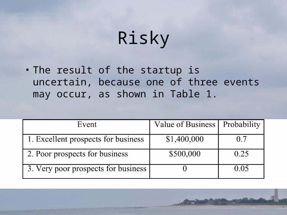
• The result of the startup is uncertain, because one of three events may occur, as shown in Table 1.

Expected Value

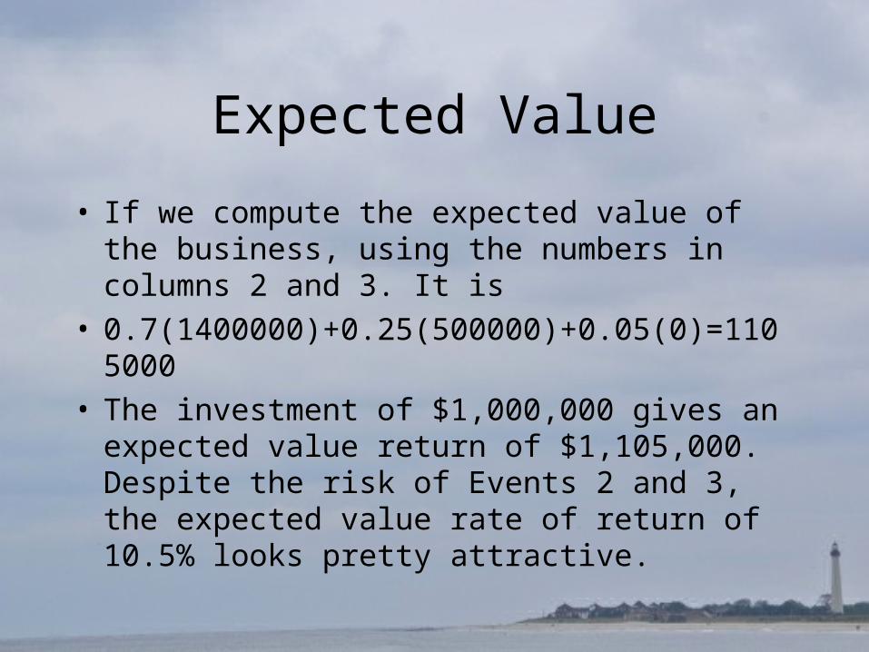
• If we compute the expected value of the business, using the numbers in columns 2 and 3. It is

• 0.7(1400000)+0.25(500000)+0.05(0)=1105000 • The investment of $1,000,000 gives an expected

value return of $1,105,000. Despite the risk of Events 2 and 3, the expected value rate of return of 10.5% looks pretty attractive.

Lender’s Risk 1.

• In order to make the $1,000,000 investment the businessperson will have to borrow some money from the banker.

• But the banker will in turn face some risk that the businessperson will become bankrupt.

Lender’s Risk 2.

• In Event 3, the businessperson certainly will be bankrupt and the bank will lose its entire loan.

• In Event 2, if the bank has leant more than $463,415, the businessperson will be bankrupt and the bank will lose some part of its loan.

Lender’s Risk 3.

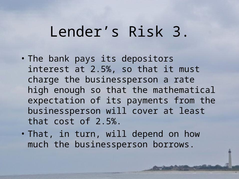
• The bank pays its depositors interest at 2.5%, so that it must charge the businessperson a rate high enough so that the mathematical expectation of its payments from the businessperson will cover at least that cost of 2.5%.

• That, in turn, will depend on how much the businessperson borrows.

Risk Premium

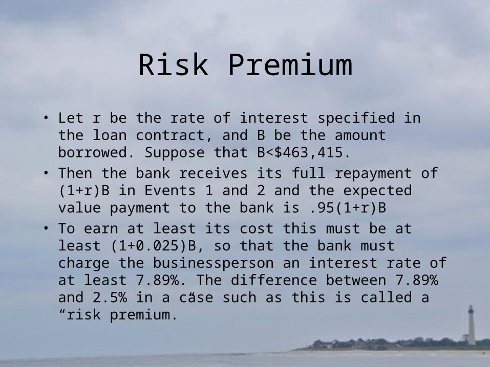
• Let r be the rate of interest specified in the loan contract, and B be the amount borrowed. Suppose that B<$463,415.

• Then the bank receives its full repayment of (1+r)B in Events 1 and 2 and the expected value payment to the bank is .95(1+r)B

• To earn at least its cost this must be at least (1+0.025)B, so that the bank must charge the businessperson an interest rate of at least 7.89%. The difference between 7.89% and 2.5% in a case such as this is called a “risk premium.”

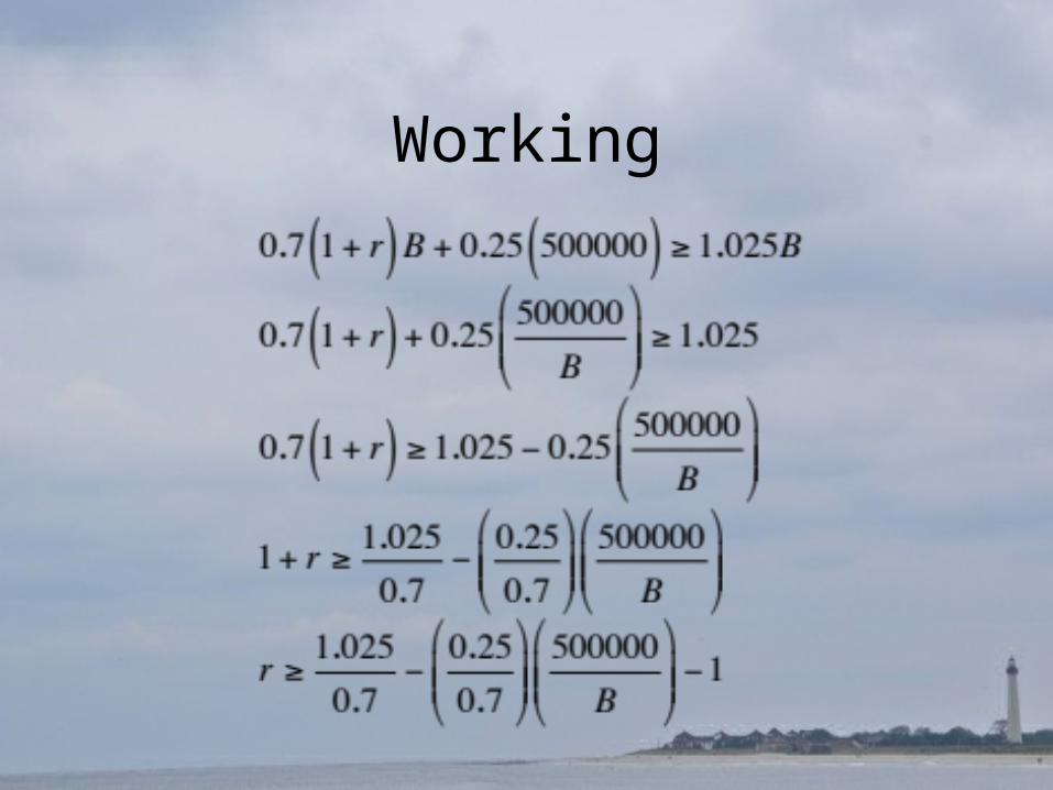
Working

• This is computed as follows:

Larger Loans 1

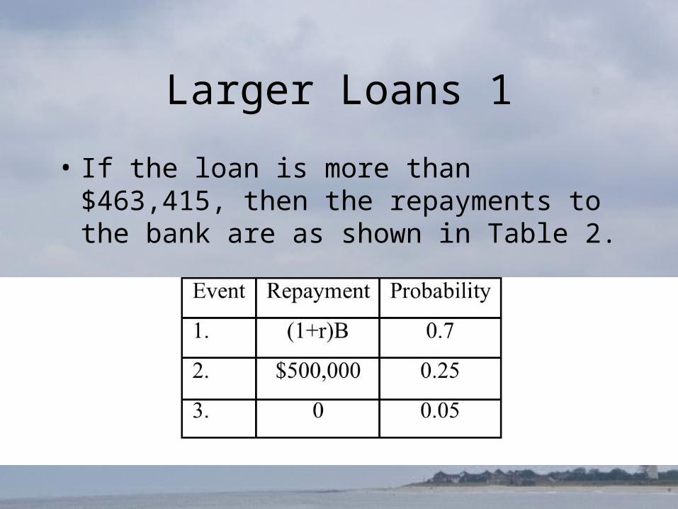
• If the loan is more than $463,415, then the repayments to the bank are as shown in Table 2.

Larger Loans 2

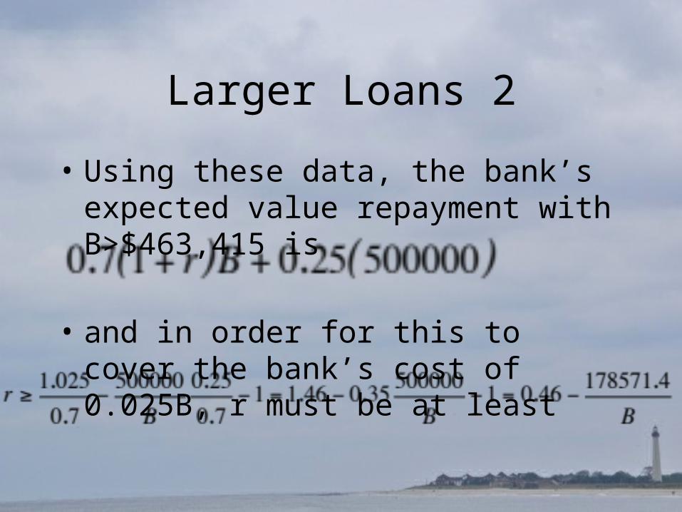
• Using these data, the bank’s expected value repayment with B>$463,415 is

• and in order for this to cover the bank’s cost of 0.025B, r must be at least

Working

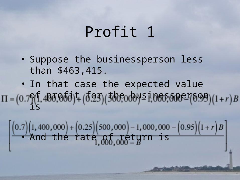
Profit 1

• Suppose the businessperson less than $463,415. • In that case the expected value of profit for the

businessperson is

• And the rate of return is

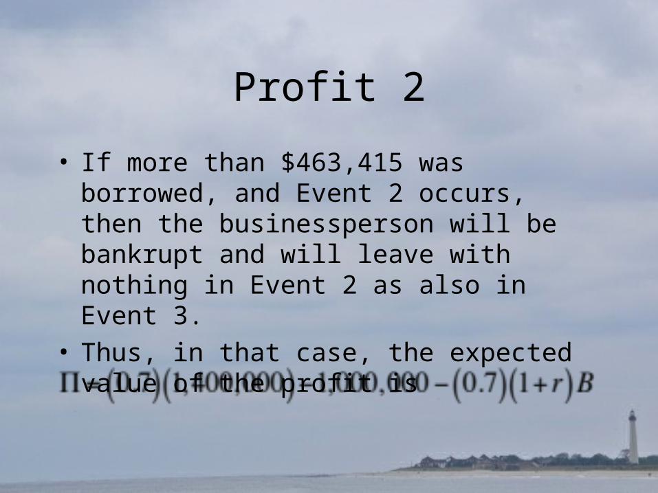
Profit 2

• If more than $463,415 was borrowed, and Event 2 occurs, then the businessperson will be bankrupt and will leave with nothing in Event 2 as also in Event 3.

• Thus, in that case, the expected value of the profit is

Profit 3

• The entrepreneur’s rate of return is

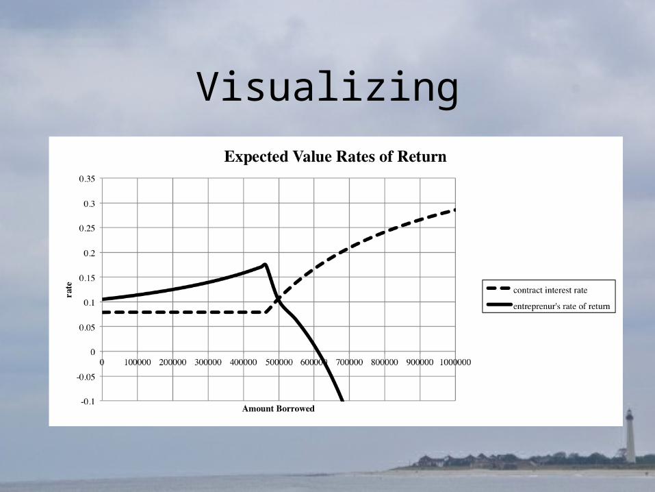
Visualizing

Discussion

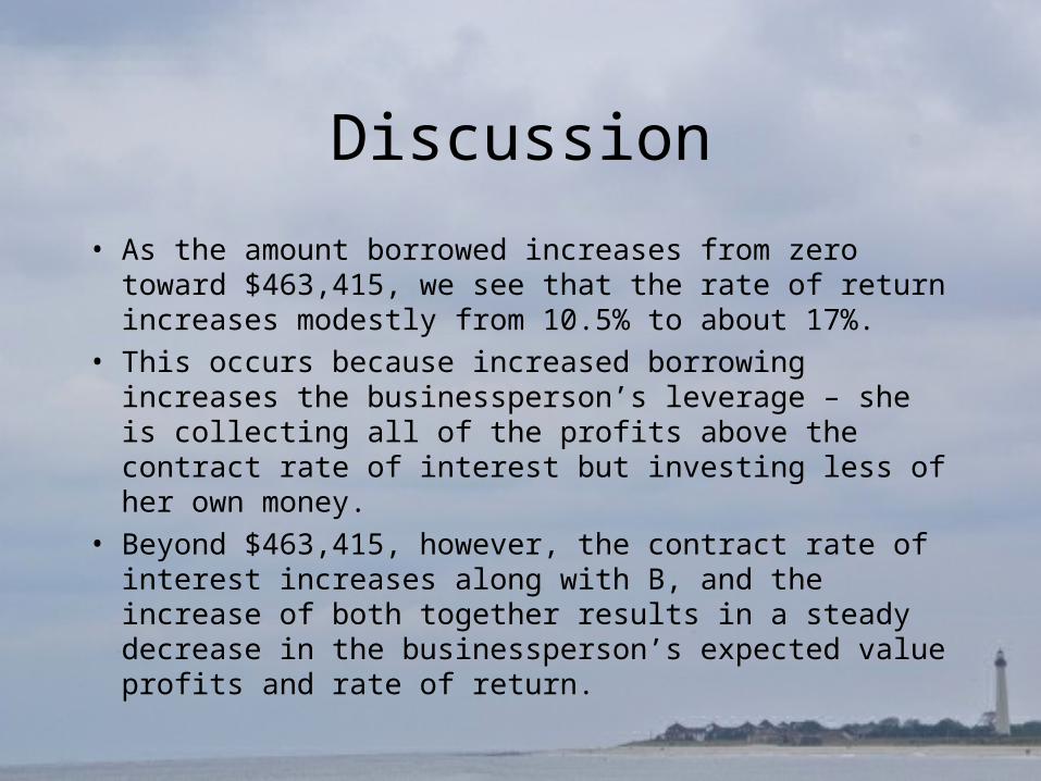
• As the amount borrowed increases from zero toward $463,415, we see that the rate of return increases modestly from 10.5% to about 17%.

• This occurs because increased borrowing increases the businessperson’s leverage – she is collecting all of the profits above the contract rate of interest but investing less of her own money.

• Beyond $463,415, however, the contract rate of interest increases along with B, and the increase of both together results in a steady decrease in the businessperson’s expected value profits and rate of return.

Liquidity Constraint 1

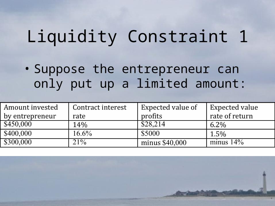
• Suppose the entrepreneur can only put up a limited amount:

Liquidity Constraint 2

• In the first case she is unable to borrow for maximum profits, and in the other two cases unable to borrow profitably at all, because she does not have enough liquid assets to invest in the project.

• A person in that situation is said to be liquidity constrained – constrained or limited by the lack of sufficient liquid assets.

Policy Conclusion?

• There is reason to think that liquidity constraint is common among small businesses, and that efficiency would be improved if small businesses as a category had more access to capital markets.

• This is debateable – my tentative opinion is that it is correct – but it is the rationale for some policies of the Small Business Administration.

2. Franchising

Franchising

• “Franchising is a system of marketing that enables firms to increase their turnover without increasing their assets.

• “Franchising involves two parties, the franchiser and the franchisee.

• “The franchiser owns a trademark or brand, which he (or she) agrees to allow the franchisee to use for a fee (often an original purchase price plus a percentage of sales).”

Ongoing

• “The franchiser provides the franchisee with assistance (financial, choice of site, and so on) in setting up their operation, and then maintains continuing control over various aspects of the franchisee’s business; for example, via the supply of products, discussion of their marketing plans and/or centralised staff training.”

Advantages

• “The franchisee buys into a proven business plan and considerable expertise. Other advantages to the franchisee include cost savings from the bulk buying capacity of a large operation, and the marketing benefits of central advertising and promotion of the business.”

Dangers

• “Some franchisers have antagonised their franchisees by selling new franchises for sites close to existing operations.”

• The franchiser might fail to maintain the brand or even go into bankruptcy.

• Franchises may have a limited term and not be renewed, or even taken over by some opportunistic employees (in a case known to me.)

Economies of Scale

• I suggest that franchising can be a way of adapting to economies of scale.

• Many businesses will require two or more business processes to be carried out in parallel.– Service provision versus national promotion, e.g.

• Franchising provides a way to have them carried out by different organizations at different scales.

Bargaining

• A franchise is a cooperative arrangement between (usually) a small and large business.

• A successful cooperative arrangement generates a surplus over what the participants could realize separately.

• This raises the question: how will the surplus be distributed among the parties?

• This is a matter of bargaining.

Economics of Bargaining 1

• Economists have been working on bargaining for about 80 years.

• Unfortunately there is no consensus theory.

• Here are a few ideas from the most widely used theory, which traces back to the Nobel Laureate game theorist John Nash.

Economics of Bargaining 2

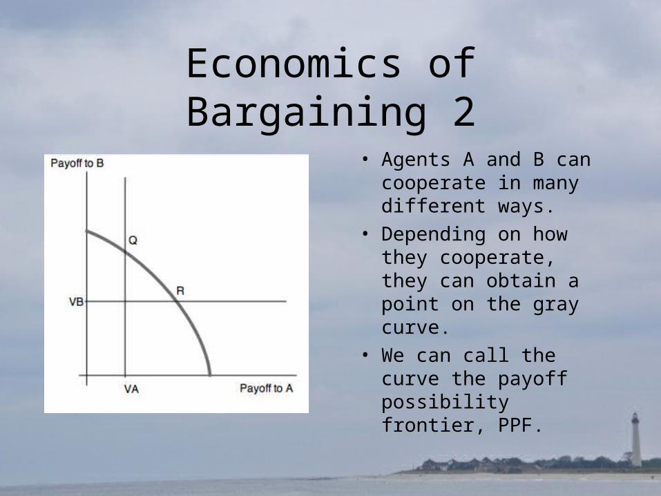
• Agents A and B can cooperate in many different ways.

• Depending on how they cooperate, they can obtain a point on the gray curve.

• We can call the curve the payoff possibility frontier, PPF.

Economics of Bargaining 3

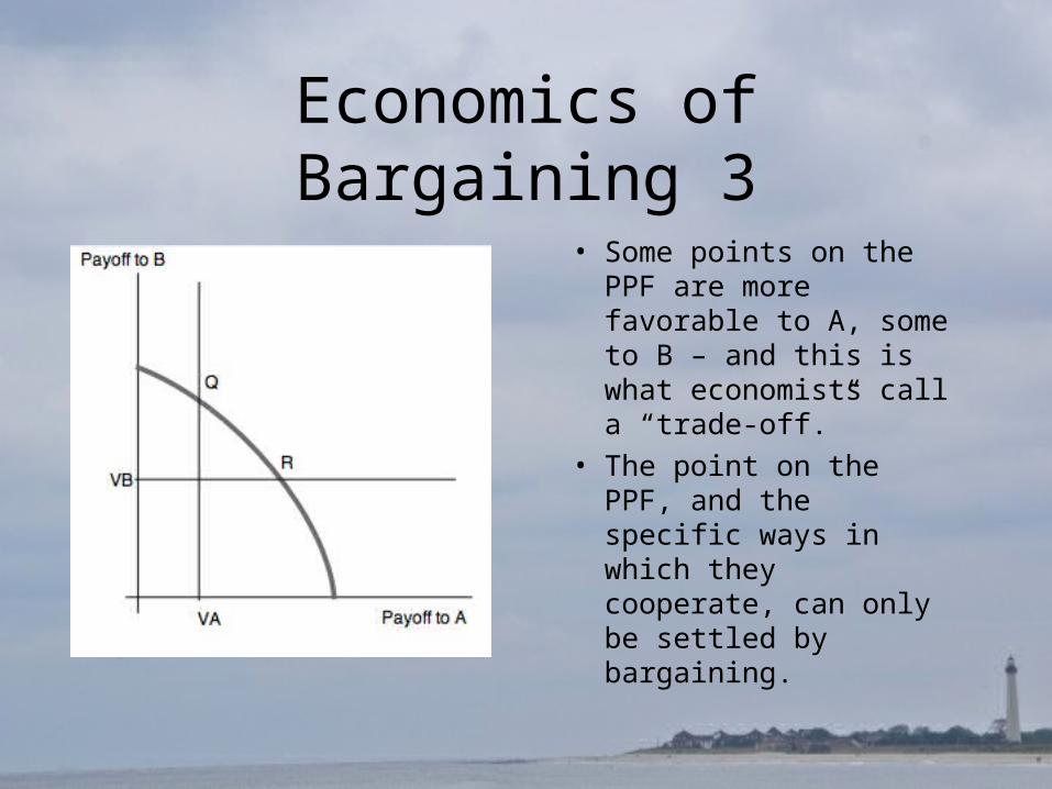
• Some points on the PPF are more favorable to A, some to B – and this is what economists call a “trade-off.”

• The point on the PPF, and the specific ways in which they cooperate, can only be settled by bargaining.

Economics of Bargaining 4

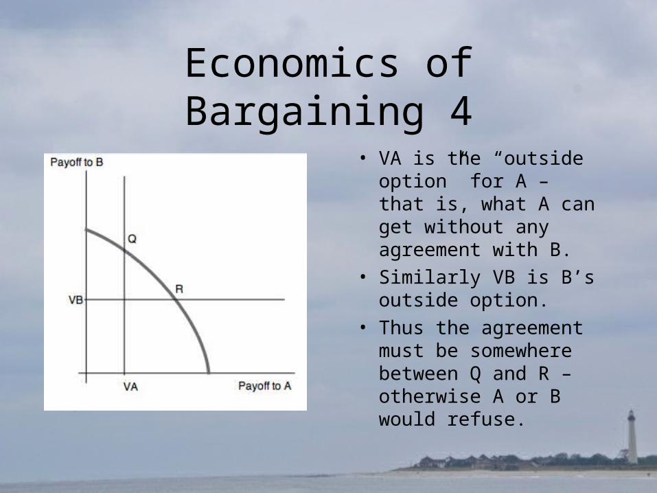
• VA is the “outside option” for A – that is, what A can get without any agreement with B.

• Similarly VB is B’s outside option.

• Thus the agreement must be somewhere between Q and R – otherwise A or B would refuse.

Bargaining Power 1

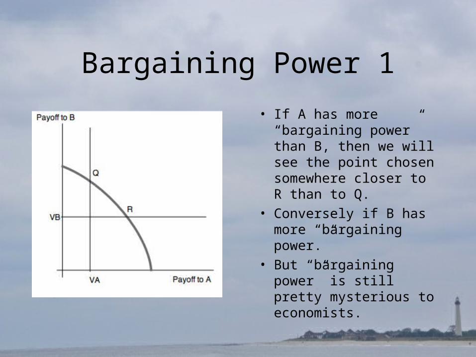
• If A has more “bargaining power” than B, then we will see the point chosen somewhere closer to R than to Q.

• Conversely if B has more “bargaining power.”

• But “bargaining power” is still pretty mysterious to economists.

Bargaining Power 2

• Here is my version:1. Bargaining power comes from threats.

2. If the bargaining is successful, the threats are not carried out, so we do not usually observe them.

3. One kind of threat – the most important kind and the only kind most theories take into account – is a threat to pull out of the agreement.

4. That would send the bargainers back to VA and VB.

5. This is the kind of threat the reading has in mind.

Reading

• The reading “Investments to create bargaining power” starts from that fact.

• It argues that some common characteristics of franchising systems reflect the attempts of the franchisors to enhance their bargaining power.

• It relies on the economics of organization approach, also known as the transaction cost approach.

Transaction Cost Approach

• Recall, this approach assumes that contracts are often incomplete (because it would be very costly to make them complete.

• Therefore 1. Opportunistic behavior may occur.

2. Conflicts over the details of the contract may occur.

3. A conflict may be resolved by renewed bargaining over the specific issue.

4. If not, a lawsuit may occur.

Opportunisms

• Opportunism may occur on either side. • The franchisor may

1. Reduce promotion and/or quality

2. Sell competing nearby franchises

3. Profit from tied sales of franchise-branded merchandise.

• The franchisee may Reduce quality and rely on customers who are

motivated by the reputation of the national brand.

How To Increase Bargaining Power 1

• According to the reading, the franchisor may increase her bargaining power by two strategies:1. “Tapered integration,” that is, owning some outlets.

2. Choosing franchisees without experience in the industry and training them.

• “Tapered integration” means the firm is partly, but not fully, vertically integrated.

• Both of these could contribute to the surplus as well as shifting bargaining power.

How To Increase Bargaining Power 2

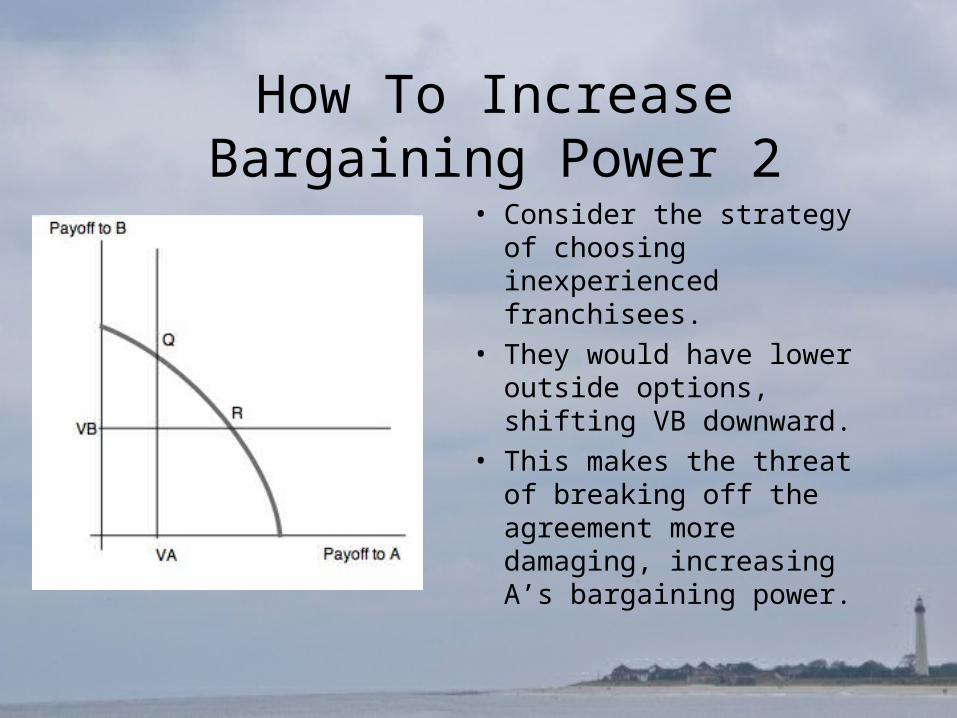
• Consider the strategy of choosing inexperienced franchisees.

• They would have lower outside options, shifting VB downward.

• This makes the threat of breaking off the agreement more damaging, increasing A’s bargaining power.

How to Increase Bargaining Power 3

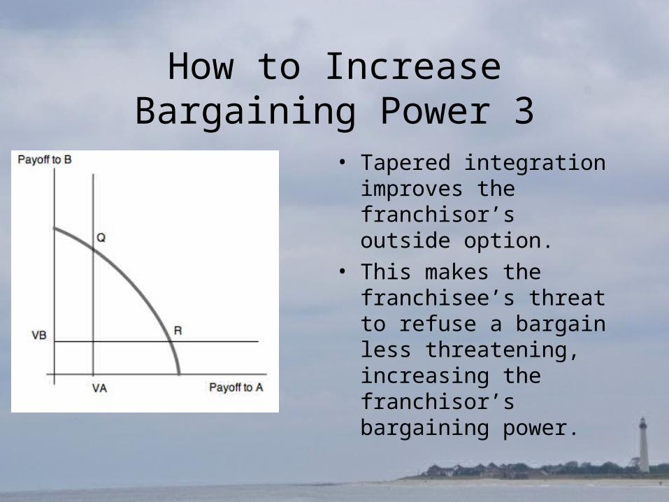
• Tapered integration improves the franchisor’s outside option.

• This makes the franchisee’s threat to refuse a bargain less threatening, increasing the franchisor’s bargaining power.

Tapered Integration

• As we see, tapered integration increases the options available to the franchisor and so increases franchisor bargaining power.

• It would also contribute to the franchisor’s experience at the retail level, enabling the franchisor to improve its service to the franchisees.

• (The reading does not point out that possibility.)

Training

• If the franchisor chooses franchisees without experience in the field, and training them, the franchisees have fewer alternatives, and thus less bargaining power.

• But training, which is the quantity used to represent this policy, will enhance franchisee productivity as well.

• (Again, the reading does not use that idea.)

How Many Lawsuits?

• The reading assumes that greater franchisor bargaining power will result in fewer lawsuits, probably because it seems that most lawsuits are filed by franchisors as a way of cancelling the franchise.

• I believe that the increased surplus that would result from the productivity effects of tapered integration and training would also lead to fewer lawsuits.

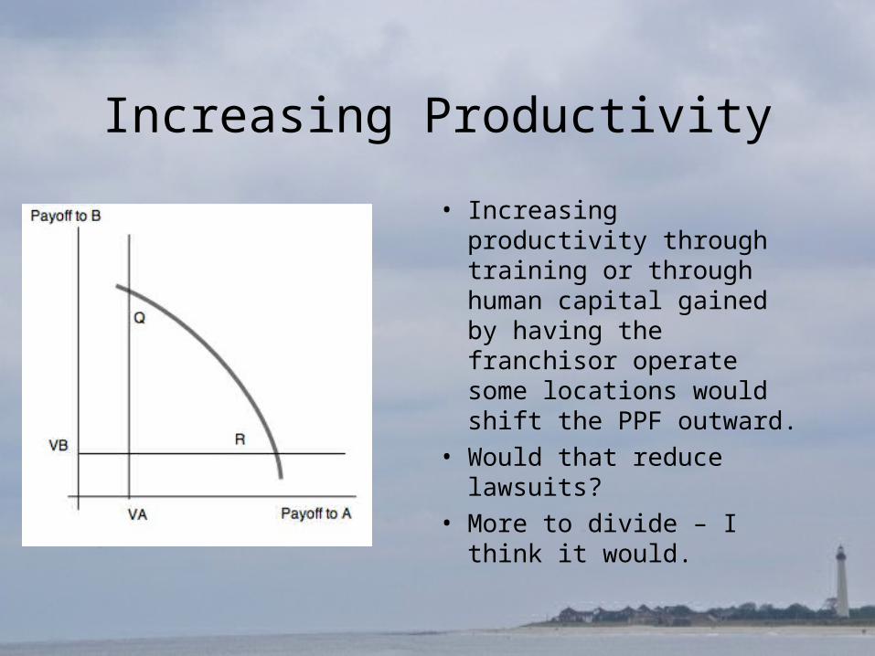
Increasing Productivity

• Increasing productivity through training or through human capital gained by having the franchisor operate some locations would shift the PPF outward.

• Would that reduce lawsuits?

• More to divide – I think it would.

Statistics 1

• Anyway, the reading uses data on the number of lawsuits over a three year period and shows that tapered integration, training, experienced franchisees, tied sales and exclusive territories have the expected influences on the number of lawsuits.

• Experienced franchisees are a key item of evidence, since they increase lawsuits but probably also increase the surplus – unlike the first two.

Statistics 2

• This study uses the negative binomial approach to the estimate, estimating the probability that there are zero, one, two, … lawsuits.

• We have seen it used before. • In this case they also estimate the dispersion – that

is, the imprecision – of the influence on the probabilities, and it seems that some are more precise than others.

Interim Conclusion

• The data are consistent with the bargaining power interpretation.

• With the exception of franchisee experience, they probably also reflect the impact of tapered integration and training on productivity.

• In any case, this study illustrates some key aspects of franchising and their consequences.

One Further Note

• Another common aspect of franchising contracts is that the fee to the franchisor often is a proportion of sales revenue, rather than a flat fee.

• Like a tax, this creates an incentive for inefficiency (another instance of opportunism.)

• Other research indicates that this will make sense only to the extent that the franchisee is liquidity-constrained.

• Conversely, franchising may open more opportunities to liquidity constrained small businesses.

Overall Conclusion• Liquidity constraint seems to be a common condition of

small businesses.

• One result of liquidity constraint is a limit to the capital scale of the enterprise.

• Thus, it is not surprising that liquidity constraint and franchising often coexist.

• Franchising permits a combination of large and small scales of operation as appropriate – with some predictable consequences.

Appendix

• The following slides are coordinated with the more advanced discussion of liquidity constraint in the optional readings “Preferences in Economic Theory” and “Borrowing for a Personal Business”

1. Capital Market Constraints

a. Review: The Indifference curve approach to saving theory

i. Review of Indifference Curves

Preference

• Recall, indifference curves are a way of expressing preference rankings.

• (They can also be derived from a utility function.)• So we begin with the concept of preference. • Preferences rank different lists or vectors of

quantities of goods, some as more desirable than others.

• Here is an example based on wings and fries.

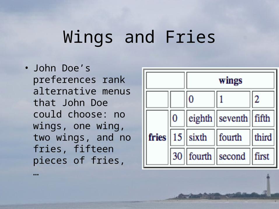
Wings and Fries

• John Doe’s preferences rank alternative menus that John Doe could choose: no wings, one wing, two wings, and no fries, fifteen pieces of fries, …

About Preferences

• This ranking illustrates some ideas from the preference approach.– First, preference is an order-ranking, not a number.

– Second, preferences are applied to combinations of the two goods.

– Third, given the amount of one good, more of the other good is preferred to less.

– When two alternatives are ranked the same, we say that the two alternatives are "indifferent choices" or "indifferent alternatives."

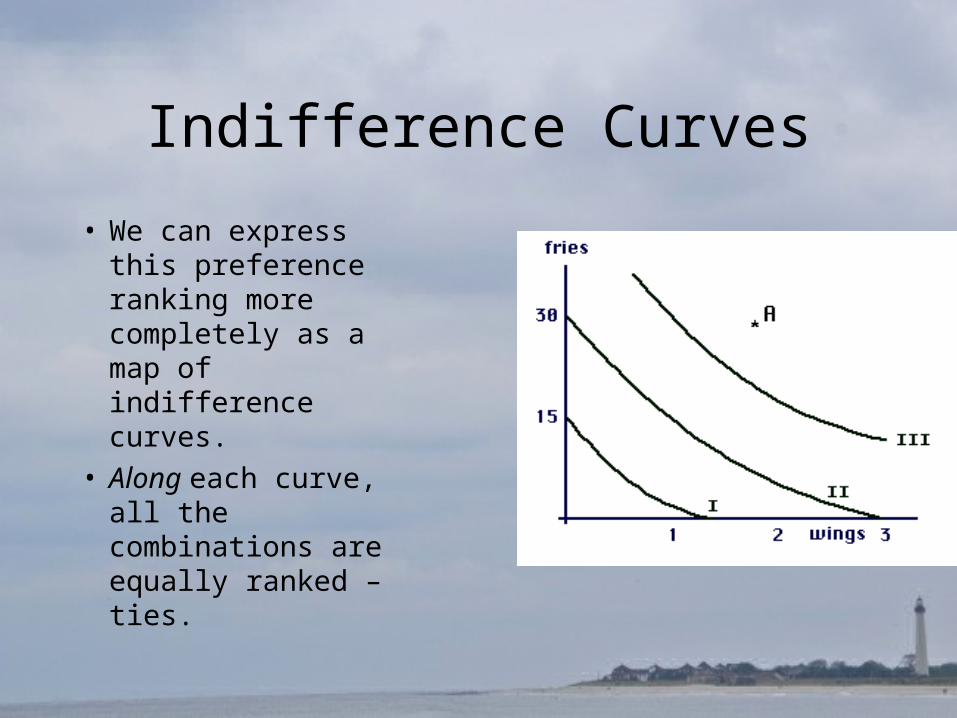
Indifference Curves

• We can express this preference ranking more completely as a map of indifference curves.

• Along each curve, all the combinations are equally ranked – ties.

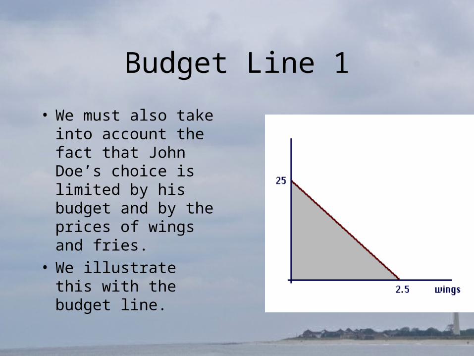
Budget Line 1

• We must also take into account the fact that John Doe’s choice is limited by his budget and by the prices of wings and fries.

• We illustrate this with the budget line.

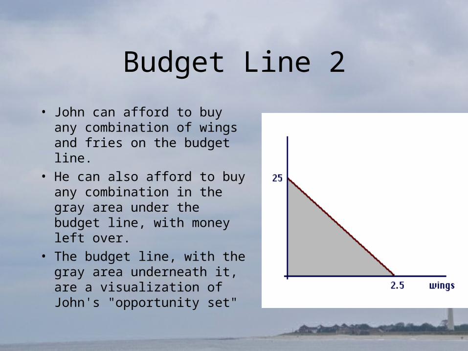
Budget Line 2

• John can afford to buy any combination of wings and fries on the budget line.

• He can also afford to buy any combination in the gray area under the budget line, with money left over.

• The budget line, with the gray area underneath it, are a visualization of John's "opportunity set"

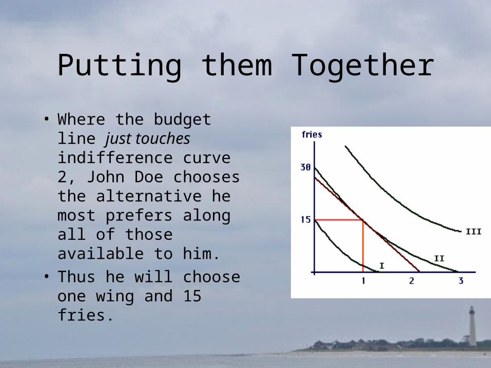
Putting them Together

• Where the budget line just touches indifference curve 2, John Doe chooses the alternative he most prefers along all of those available to him.

• Thus he will choose one wing and 15 fries.

Conclusions 1

• Here are some key conclusions from this analysis:– Since the budget line and the indifference curve are just

touching at 15 fries and 1 wing, they have the same slope, as we can see.

– The slope of the indifference curve is the marginal rate of substitution, which tells us how many fries the person is willing to give up to get one more wing.

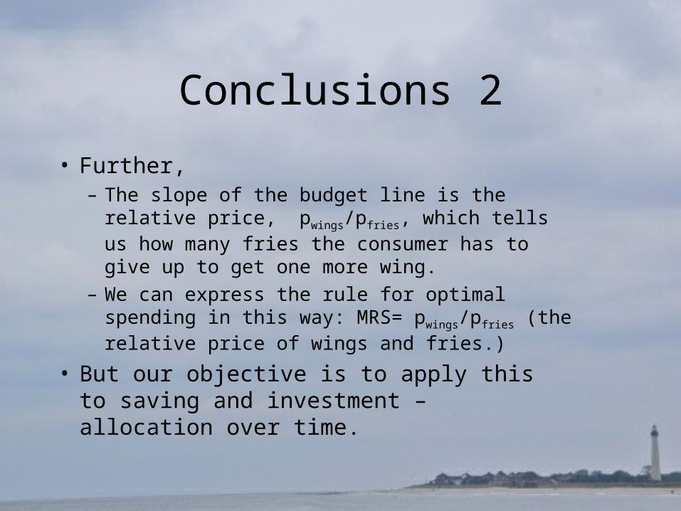
Conclusions 2

• Further, – The slope of the budget line is the relative price,

pwings/pfries, which tells us how many fries the consumer has to give up to get one more wing.

– We can express the rule for optimal spending in this way: MRS= pwings/pfries (the relative price of wings and fries.)

• But our objective is to apply this to saving and investment – allocation over time.

1. Capital Market Constraints

b. Review: The Indifference curve approach to saving theory

ii. Allocation over time

Borrowing

• Common experience tells us that small businesses often rely a great deal on borrowing, probably to a greater extent than larger businesses.

• This discussion will introduce a model of borrowing for a personal business (or for some other purposes) at the level of intermediate microeconomics.

• For this example, the individual will be trading off two goods: consumption in the current period and income in the next period.

Endowment

• Suppose the person has a certain amount of financial assets in the first period. – Call this amount M.

– Call income in the next period Y.

– Call consumption in the first period C.

Trade-offs

• There are at least two ways the person can trade off a reduction of his or her consumption in the first year to increase his or her income in the second year. – Save and make investments in financial

instruments– Save and invest in the proprietor’s own

business.

Financial Investment 1

• Suppose the rate of return on financial assets is r.

• Then every dollar set aside as financial assets in the current period will yield 1+r dollars of assets to use for consumption or other purposes in period 2.

• We can represent that aspect of the person's choice by the budget line shown in Figure 1.

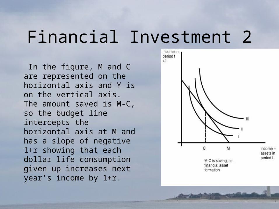
Financial Investment 2

In the figure, M and C are represented on the horizontal axis and Y is on the vertical axis. The amount saved is M-C, so the budget line intercepts the horizontal axis at M and has a slope of negative 1+r showing that each dollar life consumption given up increases next year's income by 1+r.

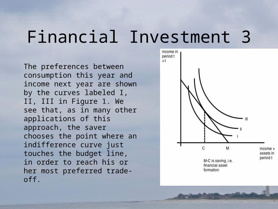
Financial Investment 3

The preferences between consumption this year and income next year are shown by the curves labeled I, II, III in Figure 1. We see that, as in many other applications of this approach, the saver chooses the point where an indifference curve just touches the budget line, in order to reach his or her most preferred trade-off.

Investment in the Business 1

• By using his or her financial assets to maintain and increase the capital stock of his or her own business, he or she may earn a better rate of return than he or she could obtain in the financial markets.

• However, this is likely to be subject to some decreasing returns.

• We have a pretty standard way of representing this in economics: a production function.

Investment in the Business 2

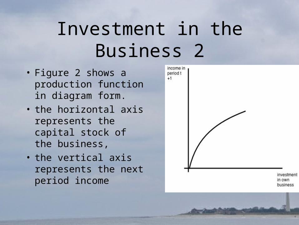
• Figure 2 shows a production function in diagram form.

• the horizontal axis represents the capital stock of the business,

• the vertical axis represents the next period income

Opportunity Set

• In Figure 3, the production function is turned around backward, intercepting the horizontal axis at consumption of M (reflecting zero investment in the business) and with income in the next period increasing step by step (with diminishing returns) as the businessperson shifts funds from first period consumption to investment.

• This shows his opportunities for consumption in this period and income in the next.

Preferences

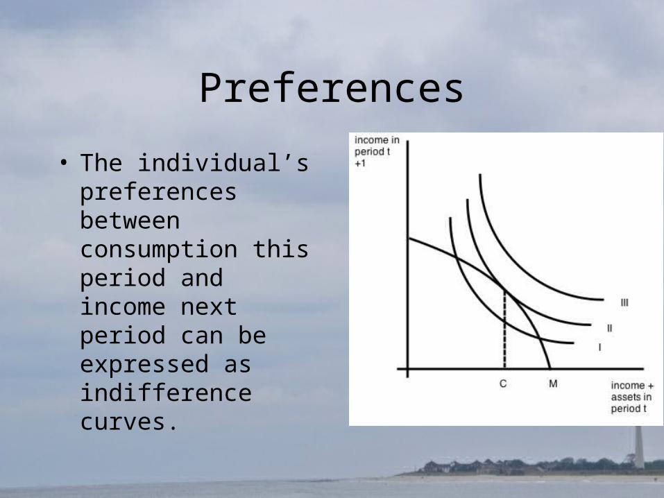
• The individual’s preferences between consumption this period and income next period can be expressed as indifference curves.

Still too Simple

• Assuming that he or she will neither borrow nor lend or invest in financial assets – for some reason he or she is isolated from financial markets – the most preferred rate of investment is the one where an indifference curve is just tangent to the possibility frontier.

• But the businessperson may also have some opportunity to participate in financial markets.

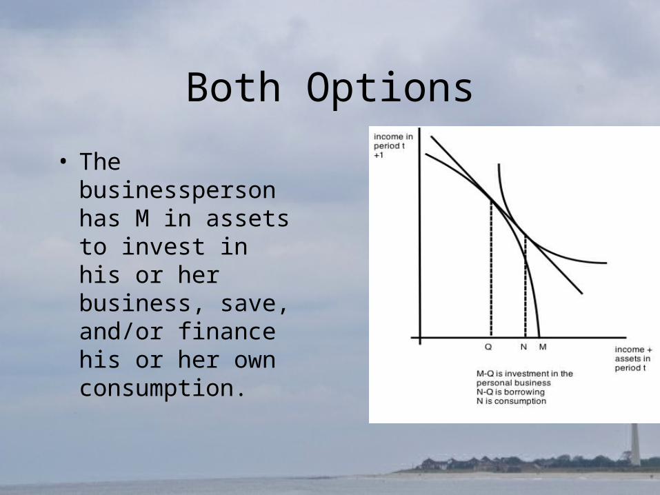
Both Options

• The businessperson has M in assets to invest in his or her business, save, and/or finance his or her own consumption.

Borrowing

• By investing in his or her own business he or she moves up the production possibility frontier to the point where the slope of the production possibility frontier is just 1+r, that is, where the marginal productivity of investment in his or her business is the same as the market rate of return.

• This is investment of M-Q. • our businessperson can now participate in capital

markets, either saving for a market rate of 1+r, or borrowing at that rate.

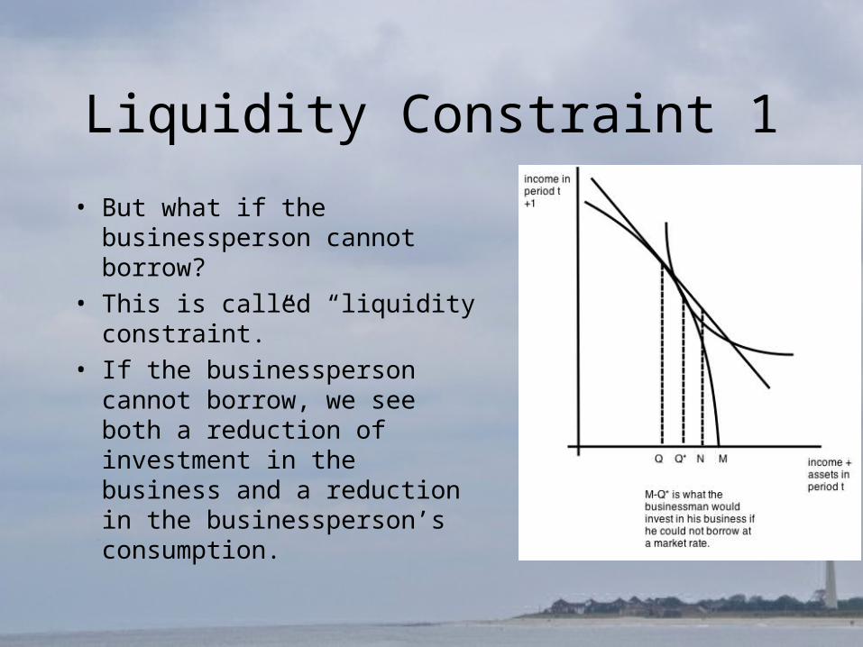
Liquidity Constraint 1

• But what if the businessperson cannot borrow?

• This is called “liquidity constraint.”

• If the businessperson cannot borrow, we see both a reduction of investment in the business and a reduction in the businessperson’s consumption.

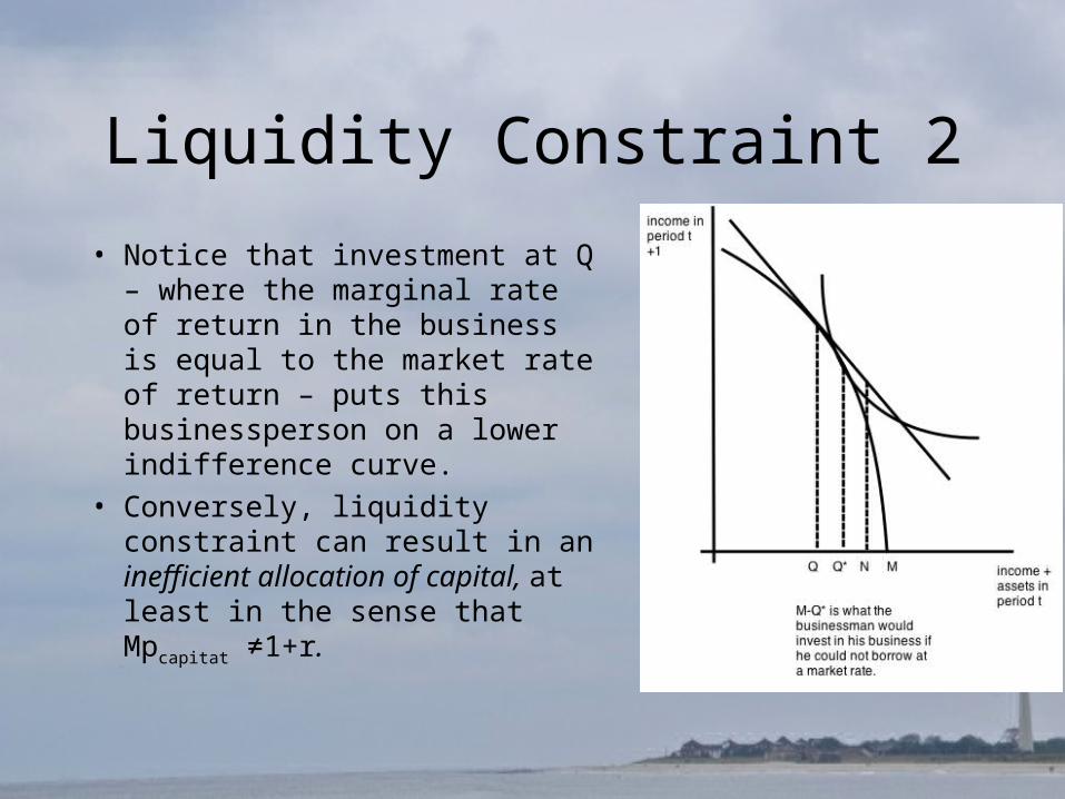
Liquidity Constraint 2

• Notice that investment at Q – where the marginal rate of return in the business is equal to the market rate of return – puts this businessperson on a lower indifference curve.

• Conversely, liquidity constraint can result in an inefficient allocation of capital, at least in the sense that Mpcapitat ≠1+r.