Embed Size (px)
Citation preview
Constraint Propagation:
The Heart of Constraint Programming
Zeynep KIZILTANDepartment of Computer Science
University of Bologna
Email: [email protected]: http://zeynep.web.cs.unibo.it/
What is it about?
4-6 hour lectures about constraint programming ingeneral and constraint propagation in specific.
– Part I: Overview of constraint programming– Part II: Constraint propagation– Part III: Some useful pointers
Aim:– Teach the basics of constraint programming.– Emphasize the importance of constraint propagation.– Point out the advanced topics.– Inform about the literature.
Warning
We will see how constraint programmingworks.
No programming examples.
PART I: Overviewof Constraint Programming
Outline
Constraint Satisfaction Problems (CSPs)
Constraint Programming (CP)– Modelling
– Backtracking Tree Search
– Local Consistency and Constraint Propagation
Constraints are everywhere!
No meetings before 9am. No registration of marks
before April 2. The lecture rooms have a
capacity. Two lectures of a student
cannot overlap. No two trains on the same
track at the same time. Salary > 45k Euros …
Constraint Satisfaction Problems
A constraint is a restriction.
There are many real-life problems that require to give adecision in the presence of constraints:
– flight / train scheduling;
– scheduling of events in an operating system;
– staff rostering at a company;
– course time tabling at a university …
Such problems are called Constraint SatisfactionProblems (CSPs).
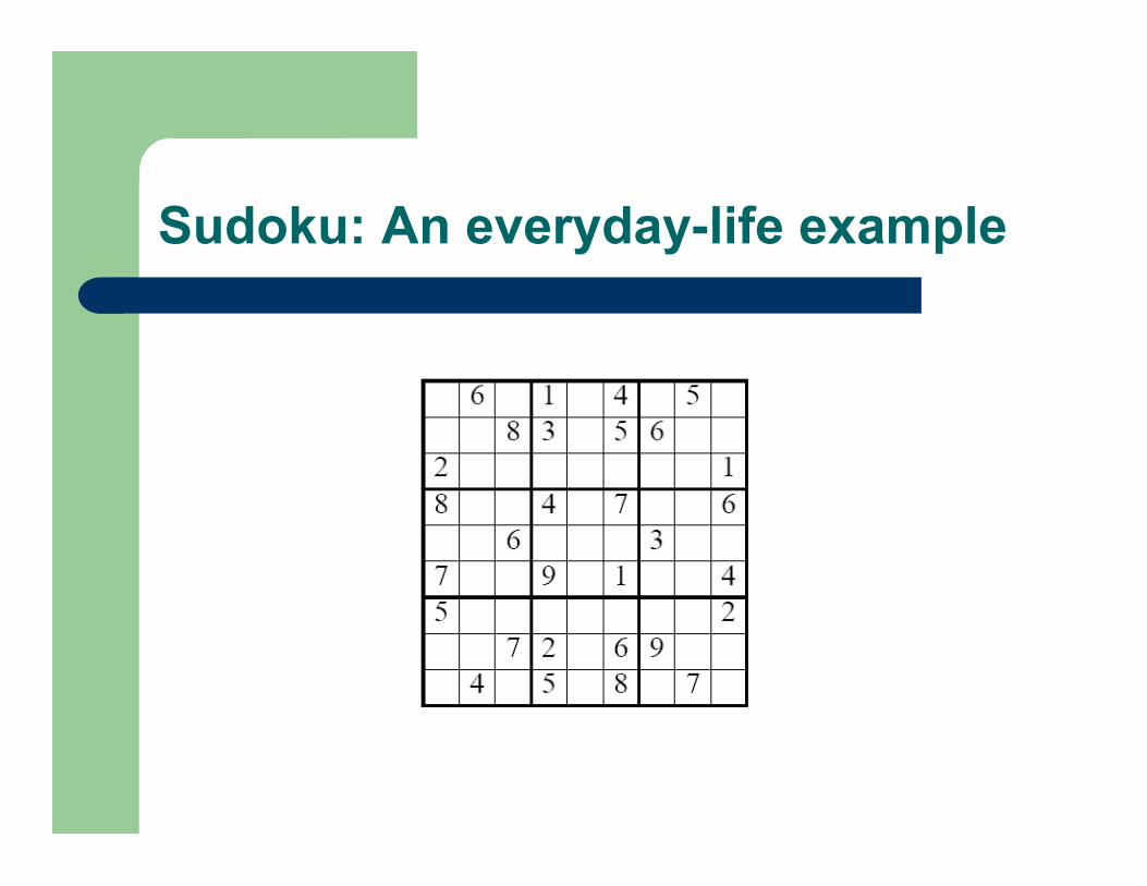
Sudoku: An everyday-life example
CSPs: More formally
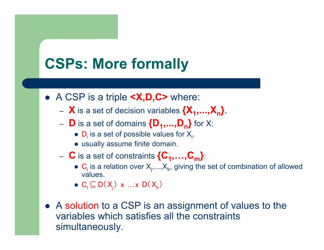
A CSP is a triple <X,D,C> where:– X is a set of decision variables {X1,...,Xn}.– D is a set of domains {D1,...,Dn} for X:
Di is a set of possible values for Xi. usually assume finite domain.
– C is a set of constraints {C1,…,Cm}: Ci is a relation over Xj,...,Xk, giving the set of combination of allowed
values. Ci ⊆ D(Xj) x . . .x D(Xk)
A solution to a CSP is an assignment of values to thevariables which satisfies all the constraintssimultaneously.
CSPs: A simple example
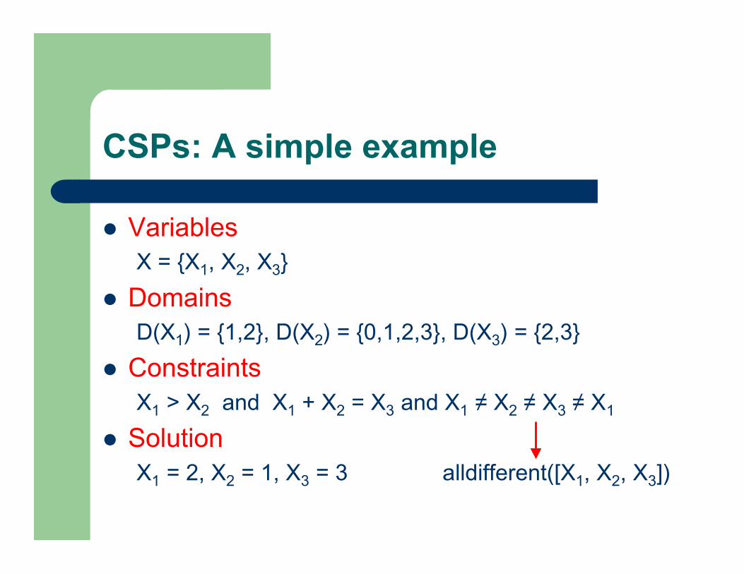
VariablesX = {X1, X2, X3}
DomainsD(X1) = {1,2}, D(X2) = {0,1,2,3}, D(X3) = {2,3}
ConstraintsX1 > X2 and X1 + X2 = X3 and X1 ≠ X2 ≠ X3 ≠ X1
SolutionX1 = 2, X2 = 1, X3 = 3 alldifferent([X1, X2, X3])
Sudoku: An everyday-life example
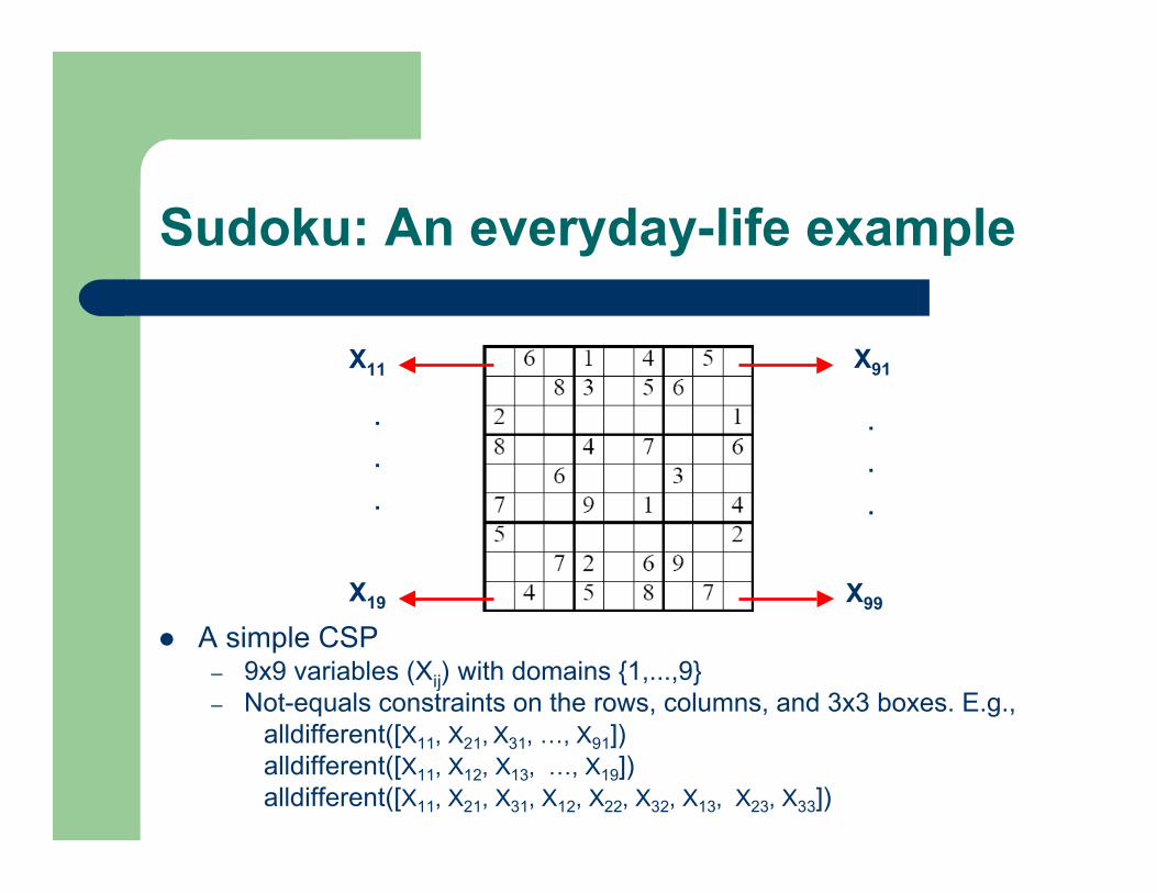
A simple CSP– 9x9 variables (Xij) with domains {1,...,9}– Not-equals constraints on the rows, columns, and 3x3 boxes. E.g.,
alldifferent([X11, X21, X31, …, X91])alldifferent([X11, X12, X13, …, X19])alldifferent([X11, X21, X31, X12, X22, X32, X13, X23, X33])
X11
.
.
.
X19 X99
.
.
.
X91
Job-Shop Scheduling: A real-life example
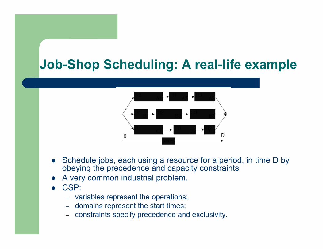
Schedule jobs, each using a resource for a period, in time D byobeying the precedence and capacity constraints
A very common industrial problem. CSP:
– variables represent the operations;– domains represent the start times;– constraints specify precedence and exclusivity.
CSPs
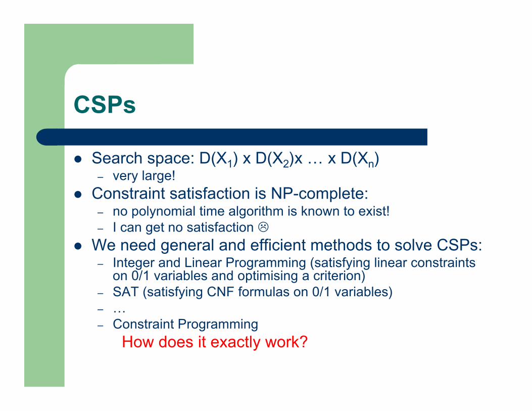
Search space: D(X1) x D(X2)x … x D(Xn)– very large!
Constraint satisfaction is NP-complete:– no polynomial time algorithm is known to exist!– I can get no satisfaction
We need general and efficient methods to solve CSPs:– Integer and Linear Programming (satisfying linear constraints
on 0/1 variables and optimising a criterion)– SAT (satisfying CNF formulas on 0/1 variables)– …– Constraint Programming
How does it exactly work?
Core of CP
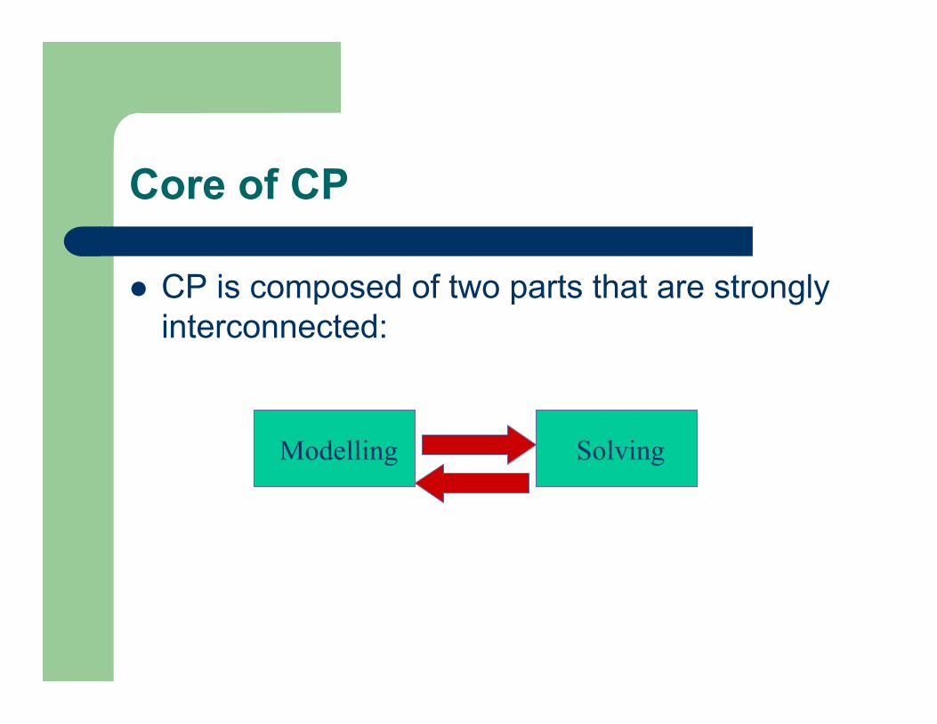
Solving Modelling
CP is composed of two parts that are stronglyinterconnected:
Core of CP-Modelling
The CP user models the problem as a CSP:– define the variables and their domains;
– specify solutions by posting constraints on thevariables: off-the-shelf constraints or user-defined constraints.
– a constraint can be thought of a reusable componentwith a propagation algorithm.
WAIT TO UNDERSTAND WHAT I MEAN
Modelling
Modelling is a critical aspect. Given the human understanding of a problem, we need
to answer questions like:– which variables shall I choose?– which constraints shall I enforce?– shall I use off-the-self constraints or define and integrate my
own?– are some constraints redundant, therefore can be avoided?– are there any implied constraints?– among alternative models, which one shall I prefer?
A problem with a simple model
X11
.
.
.
X19 X99
.
.
.
X91
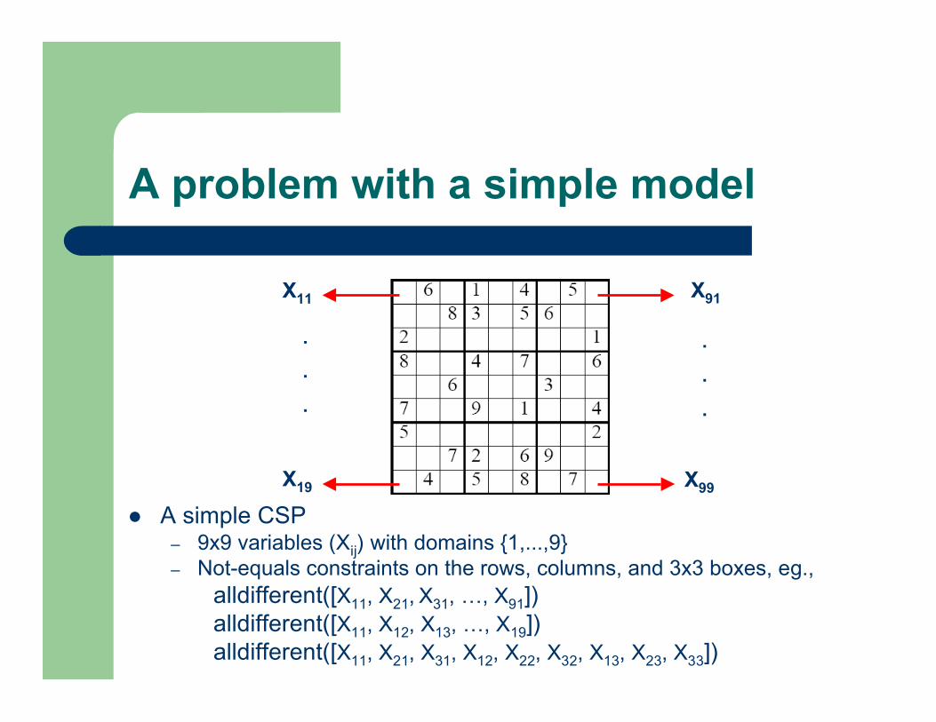
A simple CSP– 9x9 variables (Xij) with domains {1,...,9}– Not-equals constraints on the rows, columns, and 3x3 boxes, eg.,
alldifferent([X11, X21, X31, …, X91])alldifferent([X11, X12, X13, …, X19])alldifferent([X11, X21, X31, X12, X22, X32, X13, X23, X33])
A problem with a complex model
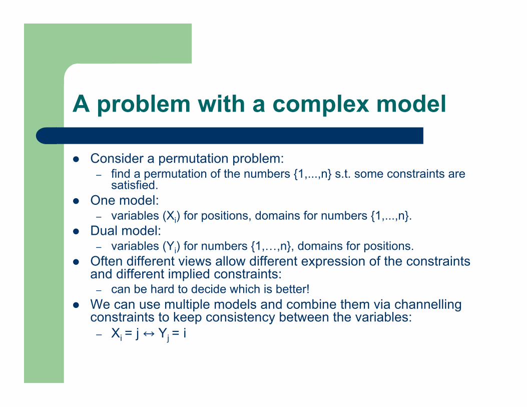
Consider a permutation problem:– find a permutation of the numbers {1,...,n} s.t. some constraints are
satisfied. One model:
– variables (Xi) for positions, domains for numbers {1,...,n}. Dual model:
– variables (Yi) for numbers {1,…,n}, domains for positions. Often different views allow different expression of the constraints
and different implied constraints:– can be hard to decide which is better!
We can use multiple models and combine them via channellingconstraints to keep consistency between the variables:
– Xi = j ↔ Yj = i
Core of CP-Solving
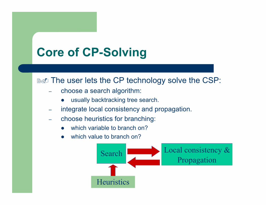
The user lets the CP technology solve the CSP:– choose a search algorithm:
usually backtracking tree search.
– integrate local consistency and propagation.
– choose heuristics for branching: which variable to branch on?
which value to branch on?
Search Local consistency & Propagation
Heuristics
Backtracking Tree Search
A possible efficient and simple method. Variables are instantiated sequentially. Whenever all the variables of a constraint is instantiated,
the validity of the constraint is checked. If a partial instantiation violates a constraint, backtracking
is performed to the most recently instantiated variablethat still has alternative values.
Backtracking eliminates a subspace from the cartesianproduct of all variable domains.
Essentially performs a depth-first search.
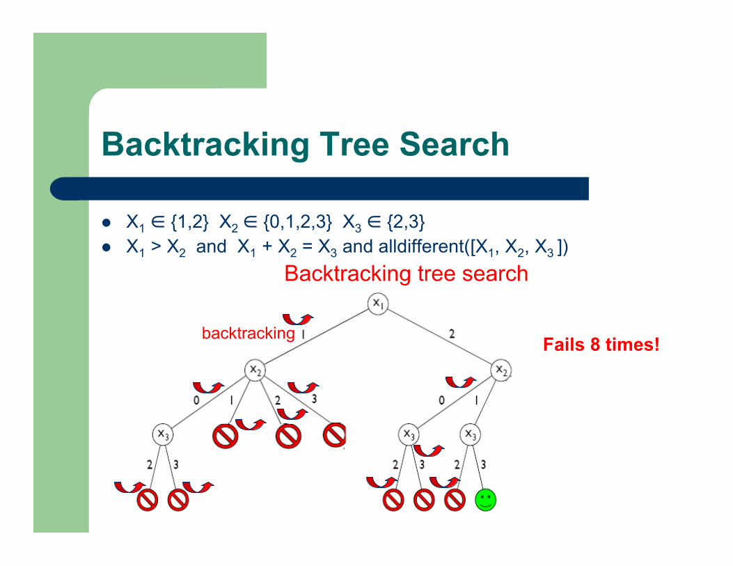
Backtracking Tree Search
X1 ∈ {1,2} X2 ∈ {0,1,2,3} X3 ∈ {2,3} X1 > X2 and X1 + X2 = X3 and alldifferent([X1, X2, X3 ])
Backtracking tree search
Fails 8 times!backtracking
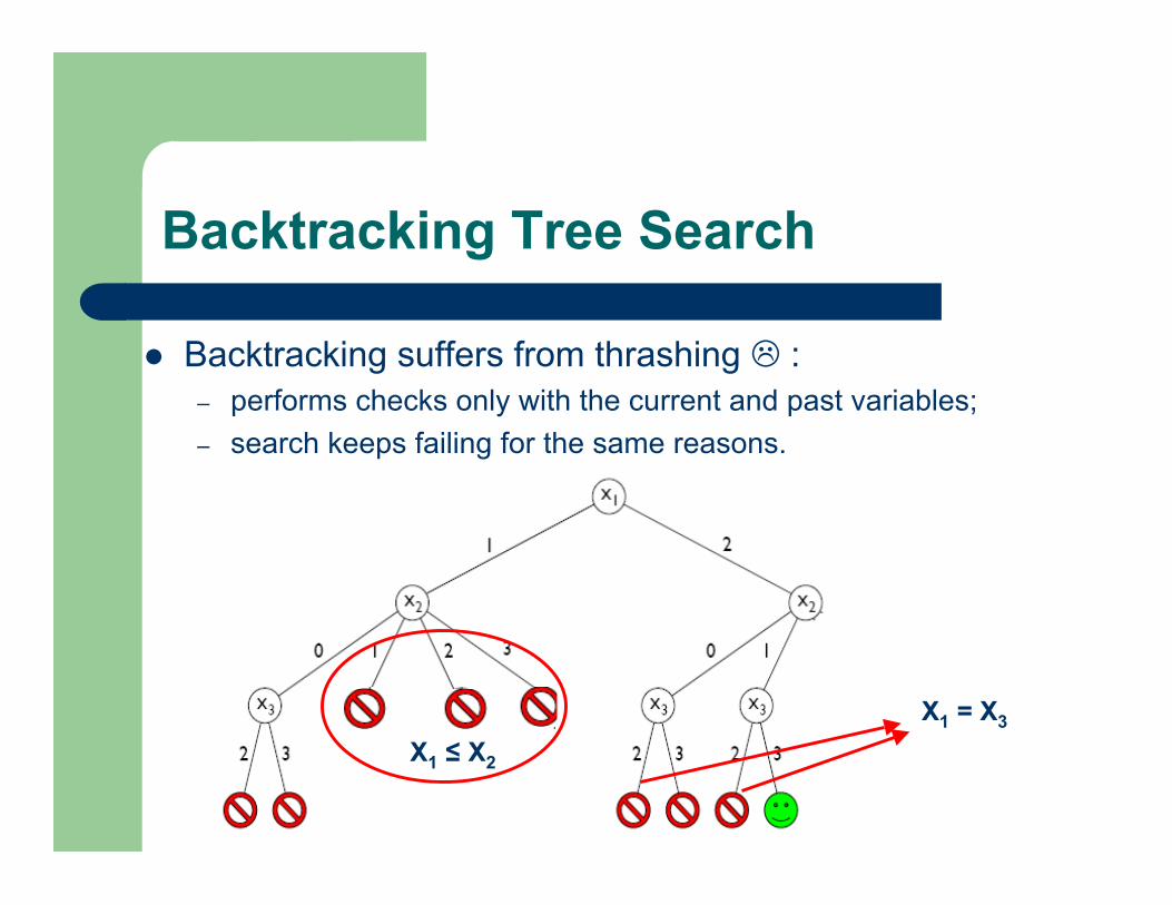
Backtracking Tree Search
Backtracking suffers from thrashing :– performs checks only with the current and past variables;
– search keeps failing for the same reasons.
X1 = X3
X1 ≤ X2
Constraint Programming
Integrates local consistency and constraintpropagation into the backtracking search.Consequently:
– we can reason about the properties of constraints and theireffect on their variables;
– some values can be filtered from some domains, reducingthe backtracking search space significantly!

Constraint Programming
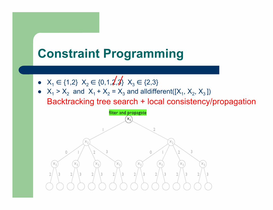
X1 ∈ {1,2} X2 ∈ {0,1,2,3} X3 ∈ {2,3} X1 > X2 and X1 + X2 = X3 and alldifferent([X1, X2, X3 ])
Backtracking tree search + local consistency/propagation
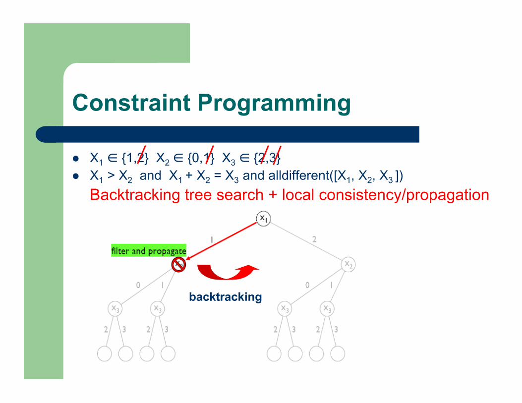
Constraint Programming
X1 ∈ {1,2} X2 ∈ {0,1} X3 ∈ {2,3} X1 > X2 and X1 + X2 = X3 and alldifferent([X1, X2, X3 ])
Backtracking tree search + local consistency/propagation
backtracking
Constraint Programming
X1 ∈ {1,2} X2 ∈ {0,1,2,3} X3 ∈ {2,3} X1 > X2 and X1 + X2 = X3 and alldifferent([X1, X2, X3 ])
Backtracking tree search + local consistency/propagation
Constraint Programming
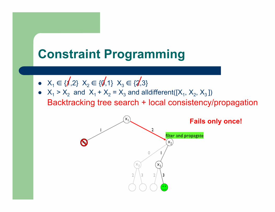
X1 ∈ {1,2} X2 ∈ {0,1} X3 ∈ {2,3} X1 > X2 and X1 + X2 = X3 and alldifferent([X1, X2, X3 ])
Backtracking tree search + local consistency/propagation
Fails only once!
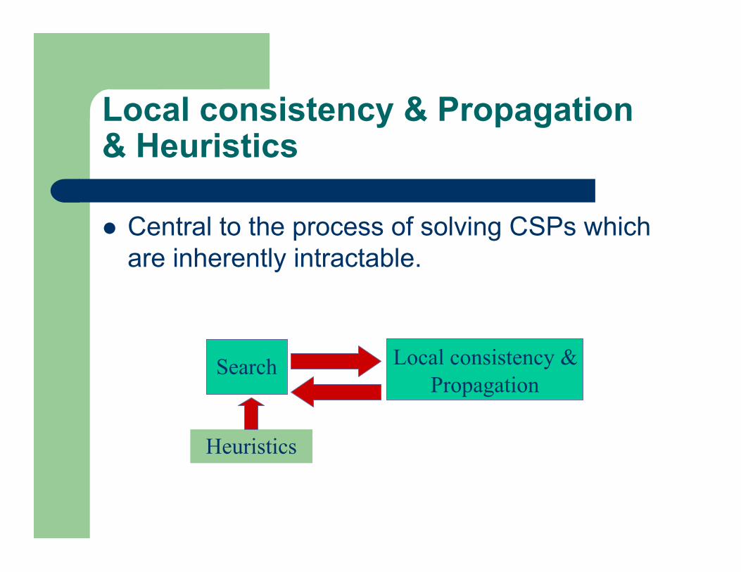
Local consistency & Propagation& Heuristics
Central to the process of solving CSPs whichare inherently intractable.
Search Local consistency & Propagation
Heuristics
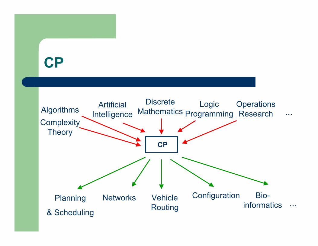
CP
Programming, in the sense of mathematicalprogramming:
– the user states declaratively the constraints on a set of decisionvariables.
– an underlying solver solves the constraints and returns asolution.
Programming, in the sense of computer programming:– the user needs to program a strategy to search for a solution.
– otherwise, solving process can be inefficient.
CP
CP
ArtificialIntelligence
DiscreteMathematics
LogicProgramming
OperationsResearchAlgorithms …
Networks VehicleRouting
Configuration Bio-informatics
Planning
& Scheduling…
ComplexityTheory

CP
Solve SUDOKU using CP!
http://www.cs.cornell.edu/gomes/SUDOKU/Sudoku.html– very easy, not worth spending minutes
– you can decide which newspaper provides the toughest Sudokuinstances
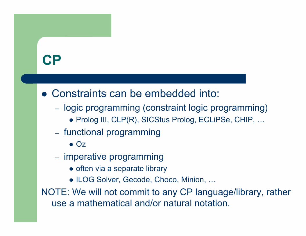
CP
Constraints can be embedded into:– logic programming (constraint logic programming)
Prolog III, CLP(R), SICStus Prolog, ECLiPSe, CHIP, …
– functional programming Oz
– imperative programming often via a separate library
ILOG Solver, Gecode, Choco, Minion, …
NOTE: We will not commit to any CP language/library, ratheruse a mathematical and/or natural notation.

PART II: Constraint Propagation
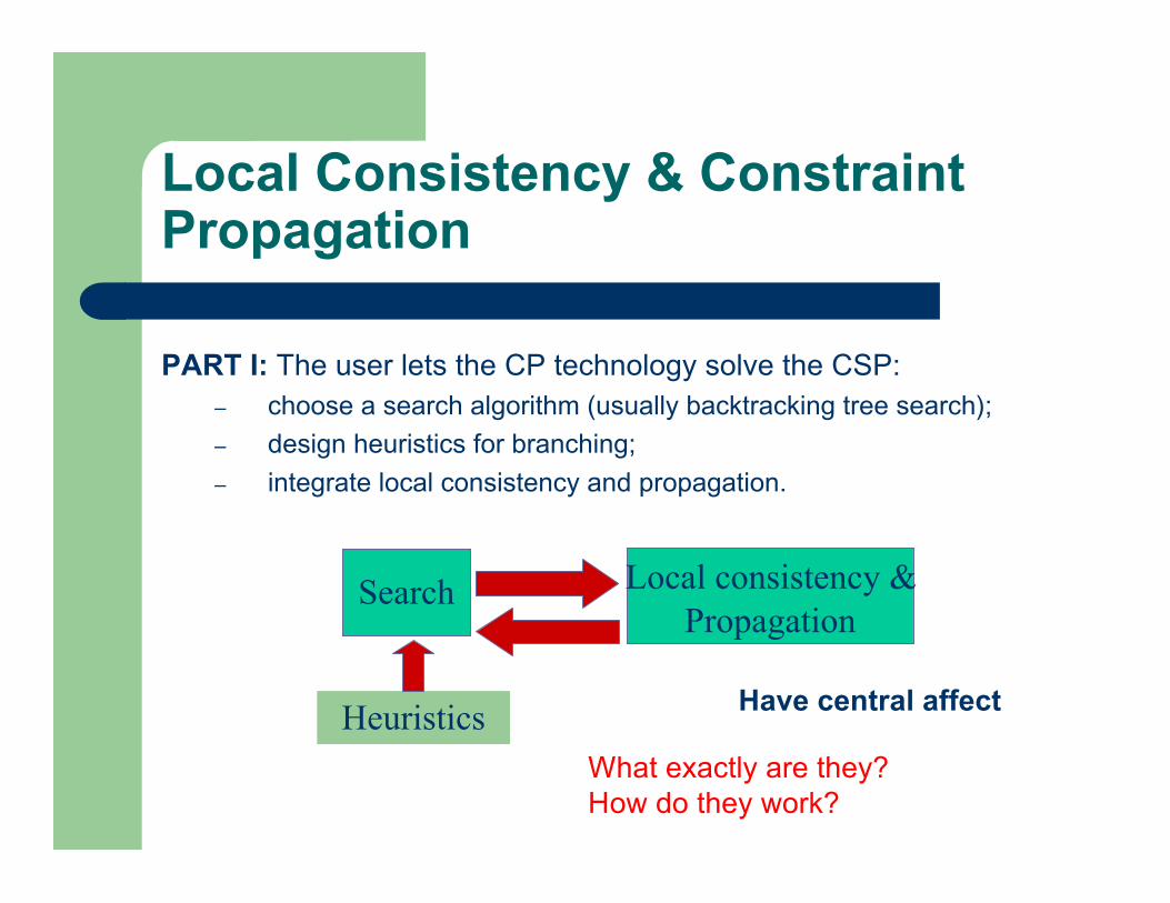
Local Consistency & ConstraintPropagation
What exactly are they?How do they work?
PART I: The user lets the CP technology solve the CSP:– choose a search algorithm (usually backtracking tree search);
– design heuristics for branching;
– integrate local consistency and propagation.
Search Local consistency & Propagation
Heuristics Have central affect
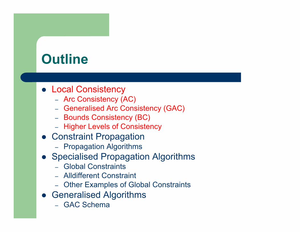
Outline
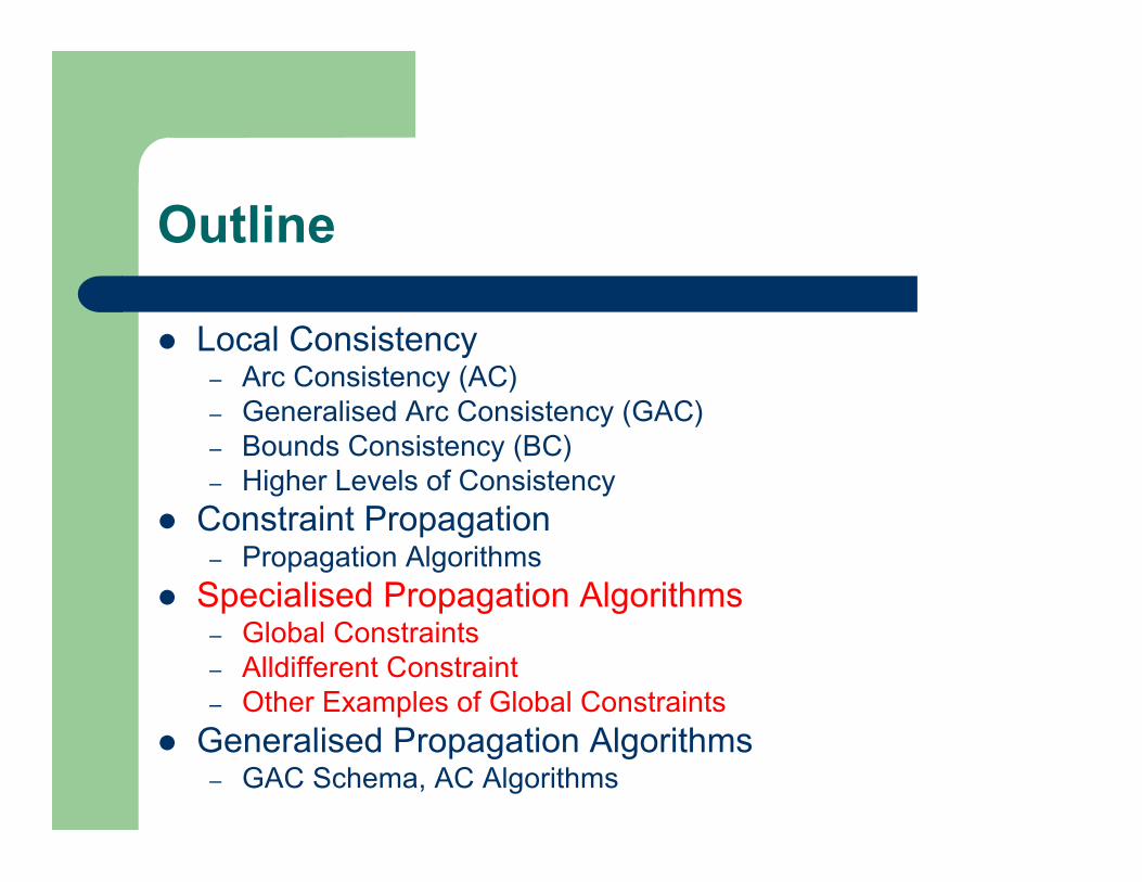
Local Consistency– Arc Consistency (AC)– Generalised Arc Consistency (GAC)– Bounds Consistency (BC)– Higher Levels of Consistency
Constraint Propagation– Propagation Algorithms
Specialised Propagation Algorithms– Global Constraints– Alldifferent Constraint– Other Examples of Global Constraints
Generalised Algorithms– GAC Schema
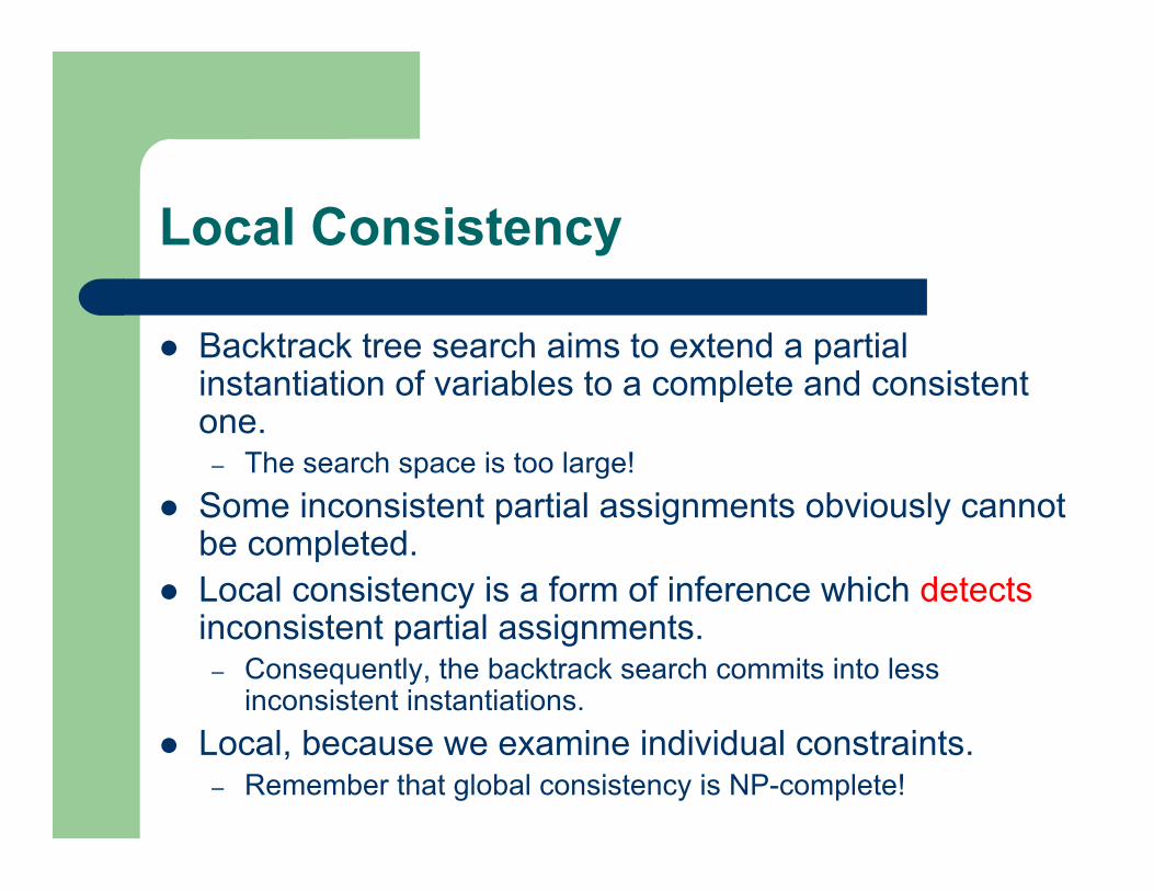
Local Consistency
Backtrack tree search aims to extend a partialinstantiation of variables to a complete and consistentone.
– The search space is too large!
Some inconsistent partial assignments obviously cannotbe completed.
Local consistency is a form of inference which detectsinconsistent partial assignments.
– Consequently, the backtrack search commits into lessinconsistent instantiations.
Local, because we examine individual constraints.– Remember that global consistency is NP-complete!
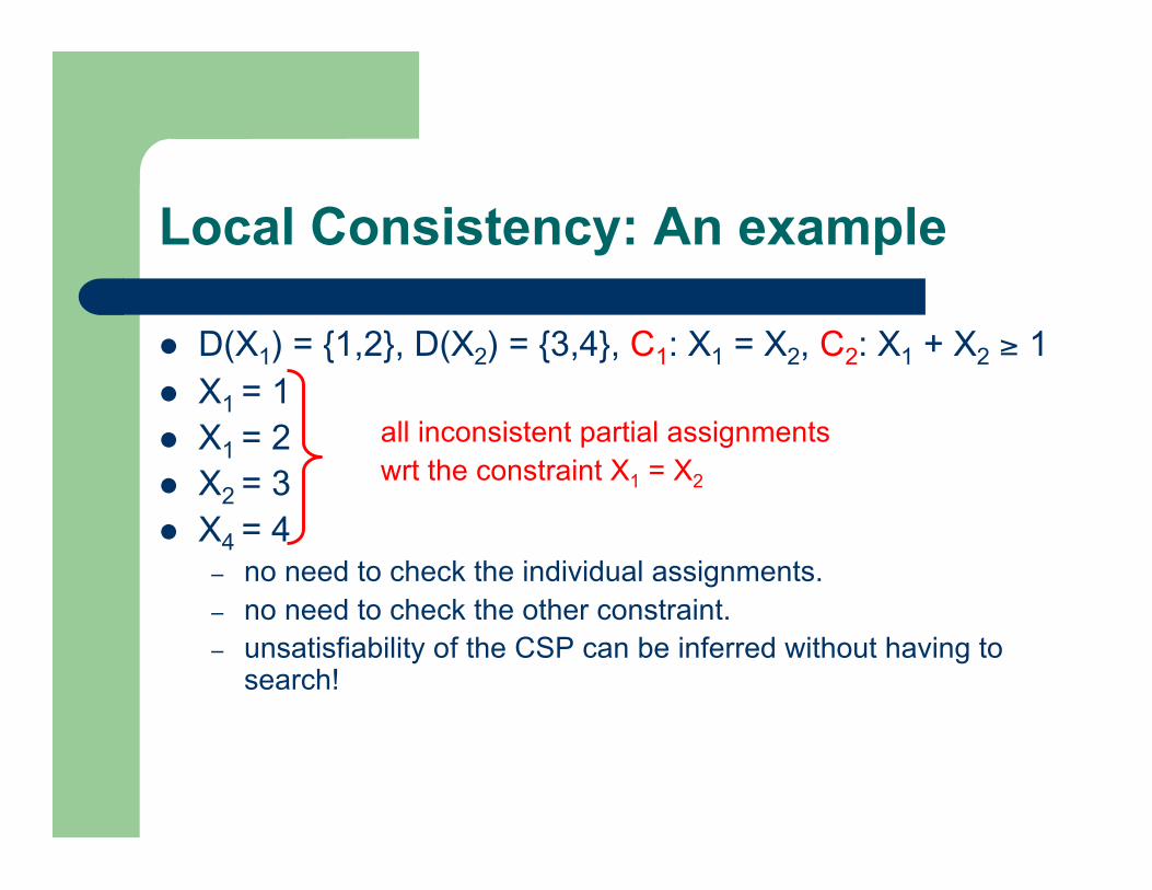
Local Consistency: An example
D(X1) = {1,2}, D(X2) = {3,4}, C1: X1 = X2, C2: X1 + X2 ≥ 1 X1 = 1 X1 = 2 X2 = 3 X4 = 4
– no need to check the individual assignments.– no need to check the other constraint.– unsatisfiability of the CSP can be inferred without having to
search!
all inconsistent partial assignmentswrt the constraint X1 = X2
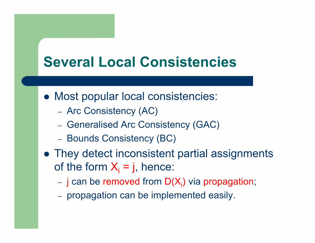
Several Local Consistencies
Most popular local consistencies:– Arc Consistency (AC)
– Generalised Arc Consistency (GAC)
– Bounds Consistency (BC)
They detect inconsistent partial assignmentsof the form Xi = j, hence:– j can be removed from D(Xi) via propagation;
– propagation can be implemented easily.
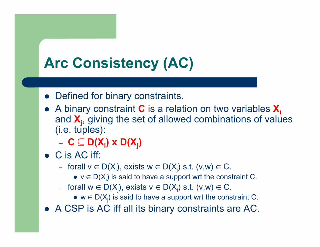
Arc Consistency (AC)
Defined for binary constraints. A binary constraint C is a relation on two variables Xi
and Xj, giving the set of allowed combinations of values(i.e. tuples): – C ⊆ D(Xi) x D(Xj)
C is AC iff:– forall v ∈ D(Xi), exists w ∈ D(Xj) s.t. (v,w) ∈ C.
v ∈ D(Xi) is said to have a support wrt the constraint C.
– forall w ∈ D(Xj), exists v ∈ D(Xi) s.t. (v,w) ∈ C. w ∈ D(Xj) is said to have a support wrt the constraint C.
A CSP is AC iff all its binary constraints are AC.
AC: An example
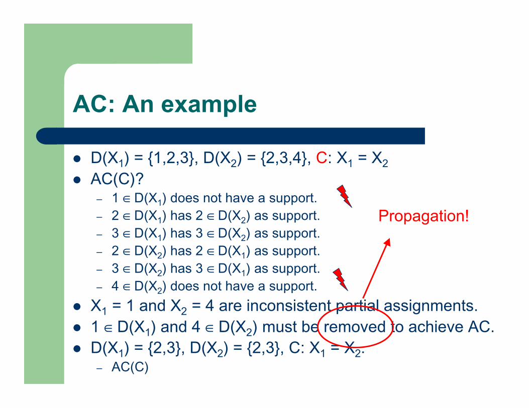
D(X1) = {1,2,3}, D(X2) = {2,3,4}, C: X1 = X2
AC(C)?– 1 ∈ D(X1) does not have a support.– 2 ∈ D(X1) has 2 ∈ D(X2) as support.– 3 ∈ D(X1) has 3 ∈ D(X2) as support.– 2 ∈ D(X2) has 2 ∈ D(X1) as support.– 3 ∈ D(X2) has 3 ∈ D(X1) as support.– 4 ∈ D(X2) does not have a support.
X1 = 1 and X2 = 4 are inconsistent partial assignments. 1 ∈ D(X1) and 4 ∈ D(X2) must be removed to achieve AC. D(X1) = {2,3}, D(X2) = {2,3}, C: X1 = X2.
– AC(C)
Propagation!
Generalised Arc Consistency
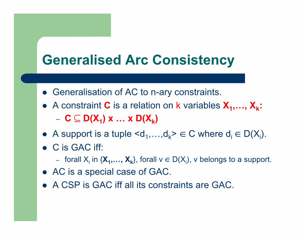
Generalisation of AC to n-ary constraints.
A constraint C is a relation on k variables X1,…, Xk:– C ⊆ D(X1) x … x D(Xk)
A support is a tuple <d1,…,dk> ∈ C where di ∈ D(Xi).
C is GAC iff:– forall Xi in {X1,…, Xk}, forall v ∈ D(Xi), v belongs to a support.
AC is a special case of GAC.
A CSP is GAC iff all its constraints are GAC.
GAC: An example
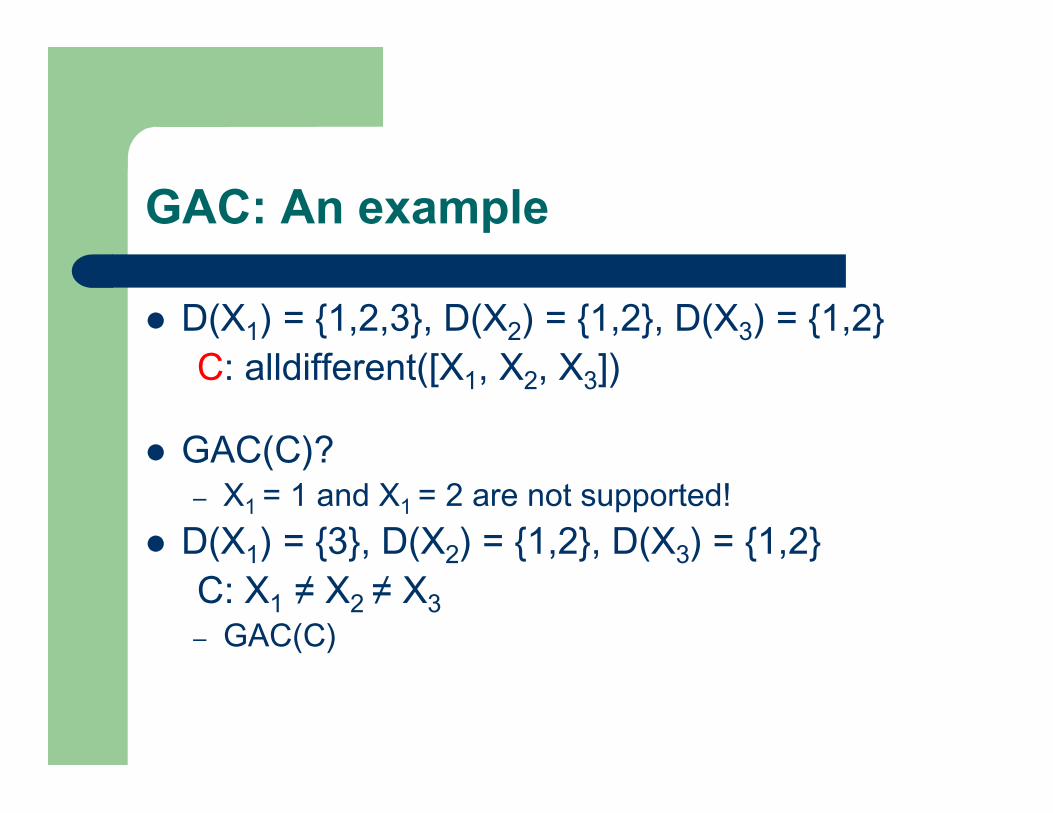
D(X1) = {1,2,3}, D(X2) = {1,2}, D(X3) = {1,2} C: alldifferent([X1, X2, X3])
GAC(C)?– X1 = 1 and X1 = 2 are not supported!
D(X1) = {3}, D(X2) = {1,2}, D(X3) = {1,2} C: X1 ≠ X2 ≠ X3
– GAC(C)
Bounds Consistency (BC)
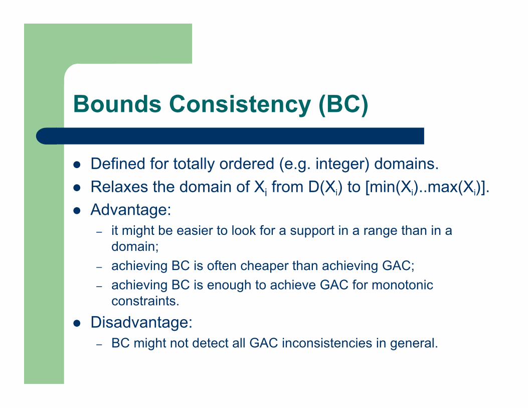
Defined for totally ordered (e.g. integer) domains.
Relaxes the domain of Xi from D(Xi) to [min(Xi)..max(Xi)].
Advantage:– it might be easier to look for a support in a range than in a
domain;
– achieving BC is often cheaper than achieving GAC;
– achieving BC is enough to achieve GAC for monotonicconstraints.
Disadvantage:– BC might not detect all GAC inconsistencies in general.
Bounds Consistency (BC)
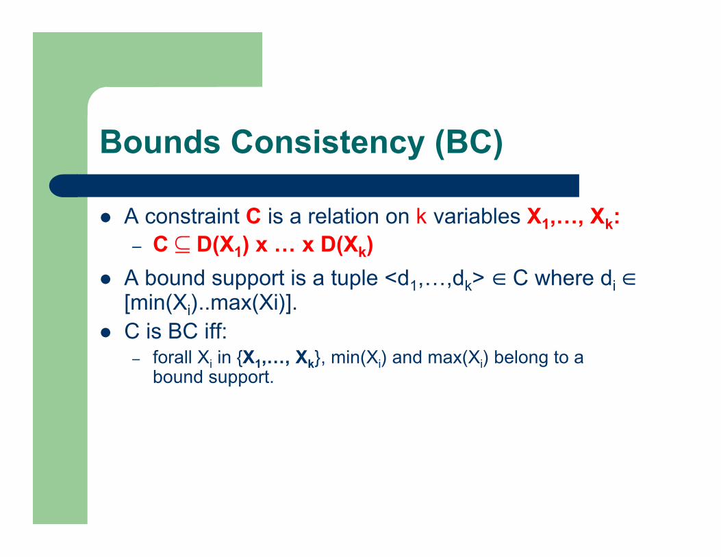
A constraint C is a relation on k variables X1,…, Xk:– C ⊆ D(X1) x … x D(Xk)
A bound support is a tuple <d1,…,dk> ∈ C where di ∈[min(Xi)..max(Xi)].
C is BC iff:– forall Xi in {X1,…, Xk}, min(Xi) and max(Xi) belong to a
bound support.
GAC > BC: An example
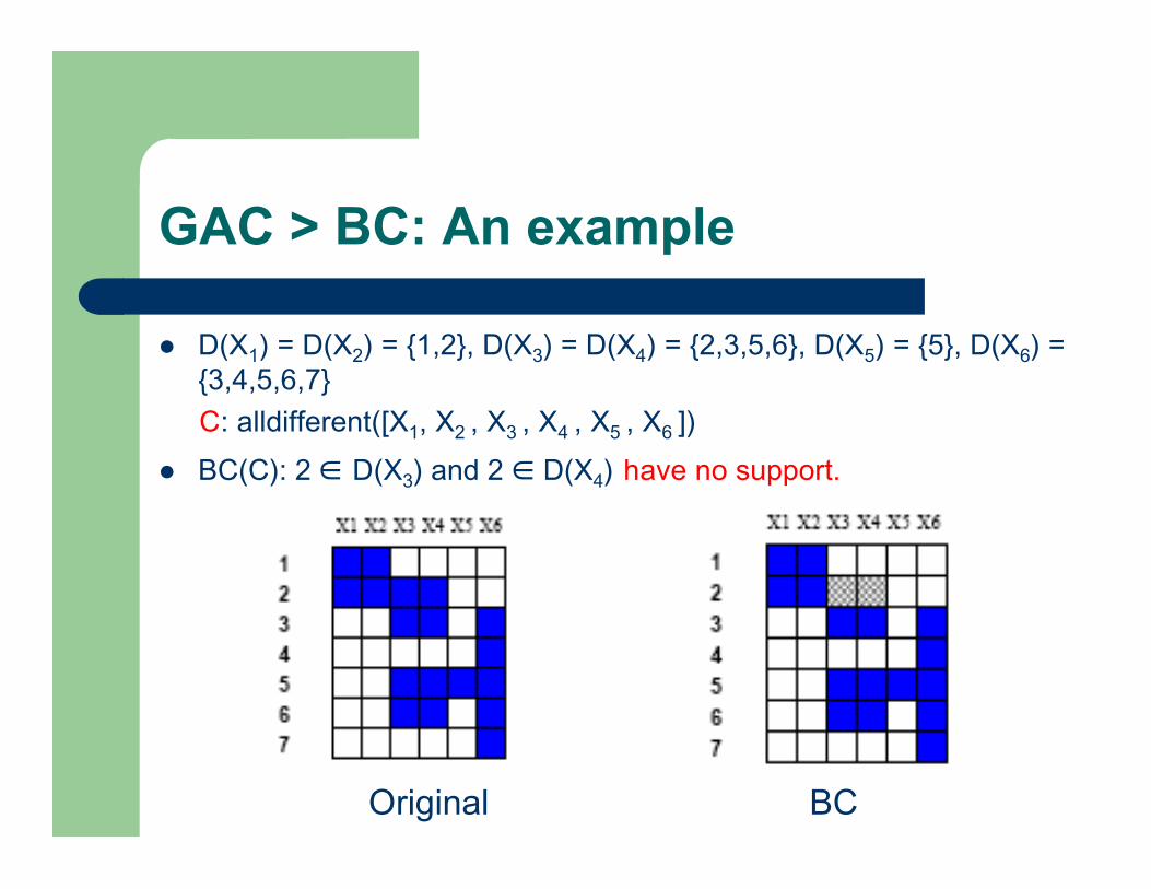
D(X1) = D(X2) = {1,2}, D(X3) = D(X4) = {2,3,5,6}, D(X5) = {5}, D(X6) ={3,4,5,6,7}
C: alldifferent([X1, X2 , X3 , X4 , X5 , X6 ])
BC(C): 2 ∈ D(X3) and 2 ∈ D(X4) have no support.
Original BC
GAC > BC: An example
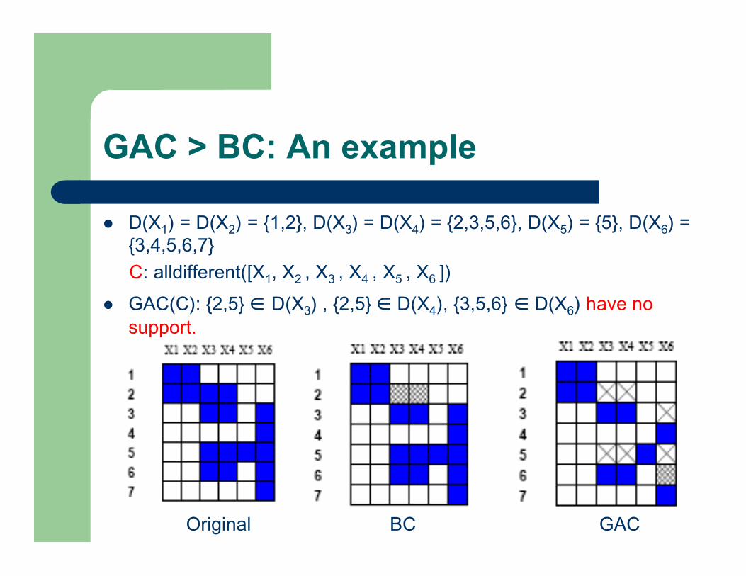
D(X1) = D(X2) = {1,2}, D(X3) = D(X4) = {2,3,5,6}, D(X5) = {5}, D(X6) ={3,4,5,6,7}
C: alldifferent([X1, X2 , X3 , X4 , X5 , X6 ])
GAC(C): {2,5} ∈ D(X3) , {2,5} ∈ D(X4), {3,5,6} ∈ D(X6) have nosupport.
Original BC GAC
GAC = BC: An example
D(X1) = {1,2,3}, D(X2) = {1,2,3}, C: X1 < X2
BC(C):– D(X1) = {1,2}, D(X2) = {2,3}
BC(C) = GAC(C):– a support for min(X2) supports all the values in D(X2).
– a support for max(X1) supports all the values in D(X1).
Higher Levels of Consistencies
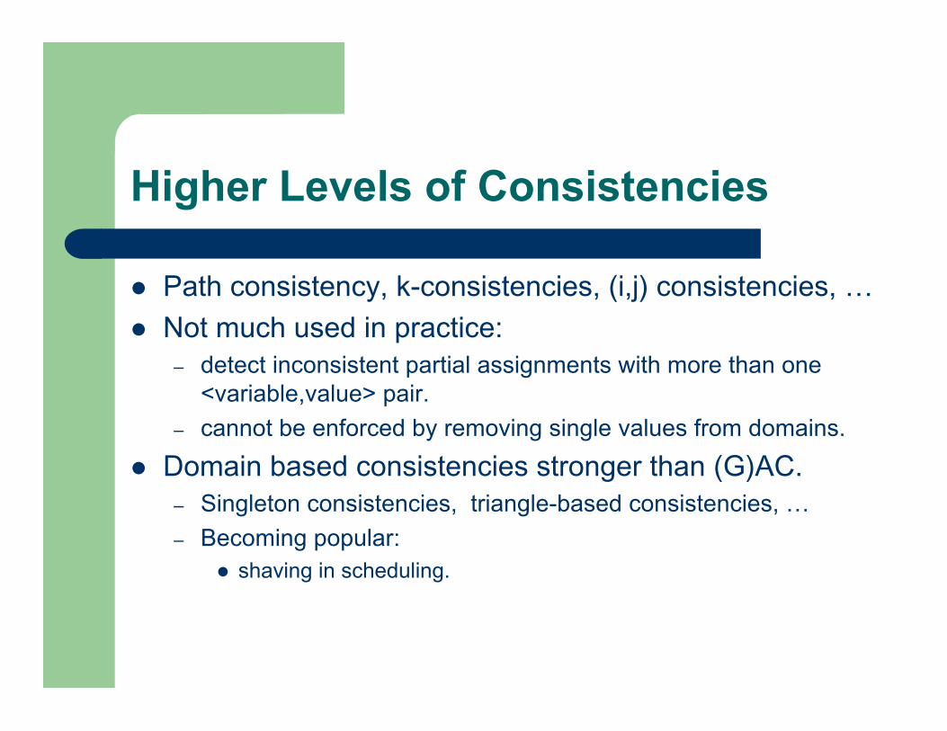
Path consistency, k-consistencies, (i,j) consistencies, …
Not much used in practice:– detect inconsistent partial assignments with more than one
<variable,value> pair.
– cannot be enforced by removing single values from domains.
Domain based consistencies stronger than (G)AC.– Singleton consistencies, triangle-based consistencies, …
– Becoming popular: shaving in scheduling.
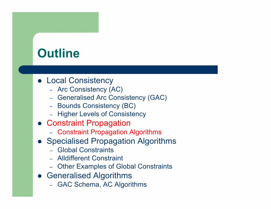
Outline
Local Consistency– Arc Consistency (AC)– Generalised Arc Consistency (GAC)– Bounds Consistency (BC)– Higher Levels of Consistency
Constraint Propagation– Constraint Propagation Algorithms
Specialised Propagation Algorithms– Global Constraints– Alldifferent Constraint– Other Examples of Global Constraints
Generalised Algorithms– GAC Schema, AC Algorithms
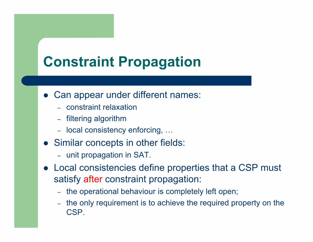
Constraint Propagation
Can appear under different names:– constraint relaxation
– filtering algorithm
– local consistency enforcing, …
Similar concepts in other fields:– unit propagation in SAT.
Local consistencies define properties that a CSP mustsatisfy after constraint propagation:
– the operational behaviour is completely left open;
– the only requirement is to achieve the required property on theCSP.
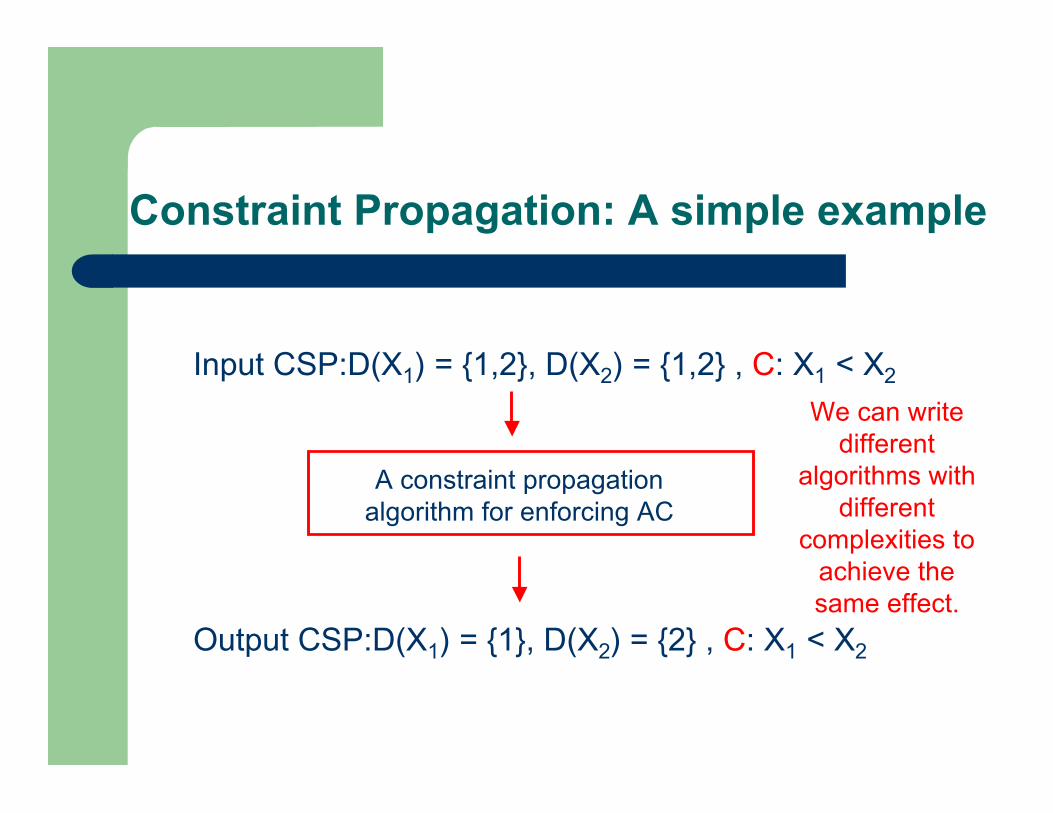
Constraint Propagation: A simple example
Input CSP:D(X1) = {1,2}, D(X2) = {1,2} , C: X1 < X2
Output CSP:D(X1) = {1}, D(X2) = {2} , C: X1 < X2
A constraint propagationalgorithm for enforcing AC
We can writedifferent
algorithms withdifferent
complexities toachieve thesame effect.
Constraint Propagation Algorithms
A constraint propagation algorithm propagates aconstraint C.– It removes the inconsistent values from the domains of
the variables of C.
– It makes C locally consistent.
– The level of consistency depends on C: GAC might be NP-complete, BC might not be possible, …
Constraint Propagation Algorithms
When solving a CSP with multiple constraints:– propagation algorithms interact;
– a propagation algorithm can wake up an alreadypropagated constraint to be propagated again!
– in the end, propagation reaches a fixed-point and allconstraints reach a level of consistency;
– the whole process is referred as constraintpropagation.
Constraint Propagation: An example
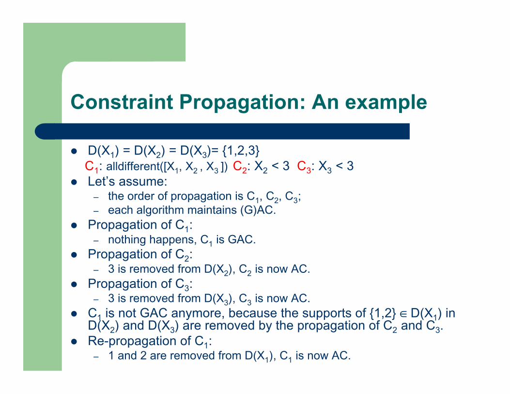
D(X1) = D(X2) = D(X3)= {1,2,3} C1: alldifferent([X1, X2 , X3 ]) C2: X2 < 3 C3: X3 < 3 Let’s assume:
– the order of propagation is C1, C2, C3;– each algorithm maintains (G)AC.
Propagation of C1:– nothing happens, C1 is GAC.
Propagation of C2:– 3 is removed from D(X2), C2 is now AC.
Propagation of C3:– 3 is removed from D(X3), C3 is now AC.
C1 is not GAC anymore, because the supports of {1,2} ∈ D(X1) inD(X2) and D(X3) are removed by the propagation of C2 and C3.
Re-propagation of C1:– 1 and 2 are removed from D(X1), C1 is now AC.
Properties of Constraint Propagation Algorithms
It is not enough to remove inconsistent values fromdomains.
A constraint propagation algorithm must wake up whennecessary, otherwise may not achieve the desired localconsistency property.
Events that trigger a constraint propagation:– when the domain of a variable changes;
– when one variable is assigned a value;
– when the minimum or the maximum values of a domain changes.
Outline
Local Consistency– Arc Consistency (AC)– Generalised Arc Consistency (GAC)– Bounds Consistency (BC)– Higher Levels of Consistency
Constraint Propagation– Propagation Algorithms
Specialised Propagation Algorithms– Global Constraints– Alldifferent Constraint– Other Examples of Global Constraints
Generalised Propagation Algorithms– GAC Schema, AC Algorithms
Specialised Propagation Algorithms
A constraint propagation algorithm can be general orspecialised:
– general, if it is applicable to any constraint;
– specialised, if it is specific to a constraint, exploiting the constraintsemantics.
Many real-life constraints are complex and non-binary.
A global constraint is a complex and non-binaryconstraint which encapsulates a specialised propagationalgorithm.
Benefits of Global Constraints
Modelling benefits– Reduce the gap between the problem statement and the
model.
– Capture recurring modelling patterns.
– May allow the expression of constraints that are otherwisenot possible to state using primitive constraints (semantic).
Solving benefits– More inference in propagation (operational).
– More efficient propagation (algorithmic).
Alldifferent Constraint
Alldifferent constraint– useful in a variety of assignment problems
e.g. permutation, timetabling, production problems, …
– alldifferent ([X1, X2, …, Xn]) holds iff
Xi ≠ Xj forall i < j ∈ {1,…,n}
Alldifferent Constraint
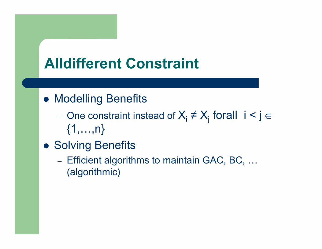
Modelling Benefits
– One constraint instead of Xi ≠ Xj forall i < j ∈{1,…,n}
Solving Benefits– Efficient algorithms to maintain GAC, BC, …
(algorithmic)
Alldifferent Constraint
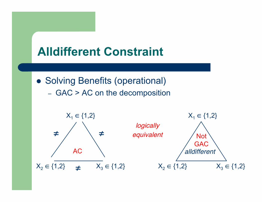
logicallyequivalent≠ ≠
≠ alldifferent
Solving Benefits (operational)– GAC > AC on the decomposition
AC
NotGAC
X1 ∈ {1,2}
X2 ∈ {1,2} X3 ∈ {1,2}
X1 ∈ {1,2}
X2 ∈ {1,2} X3 ∈ {1,2}
Alldifferent Constraint
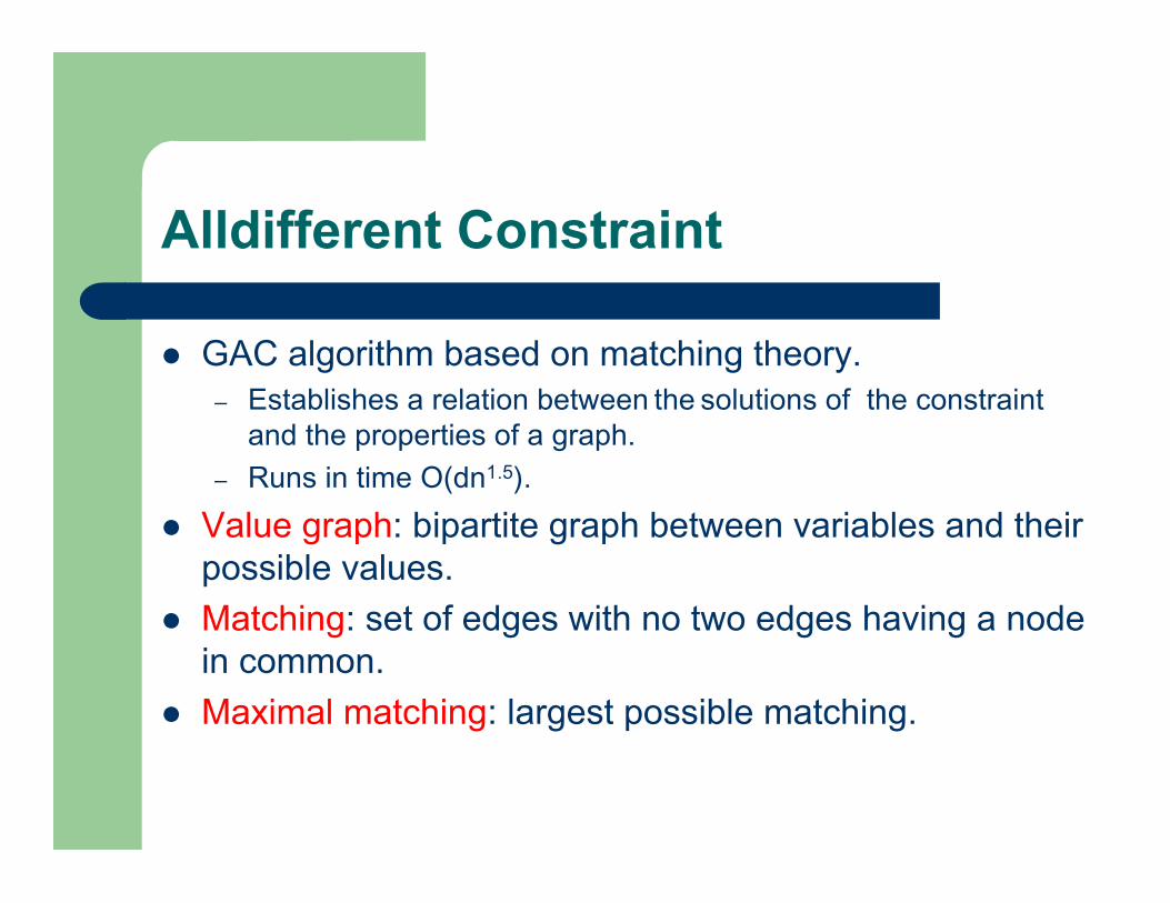
GAC algorithm based on matching theory.– Establishes a relation between the solutions of the constraint
and the properties of a graph.
– Runs in time O(dn1.5).
Value graph: bipartite graph between variables and theirpossible values.
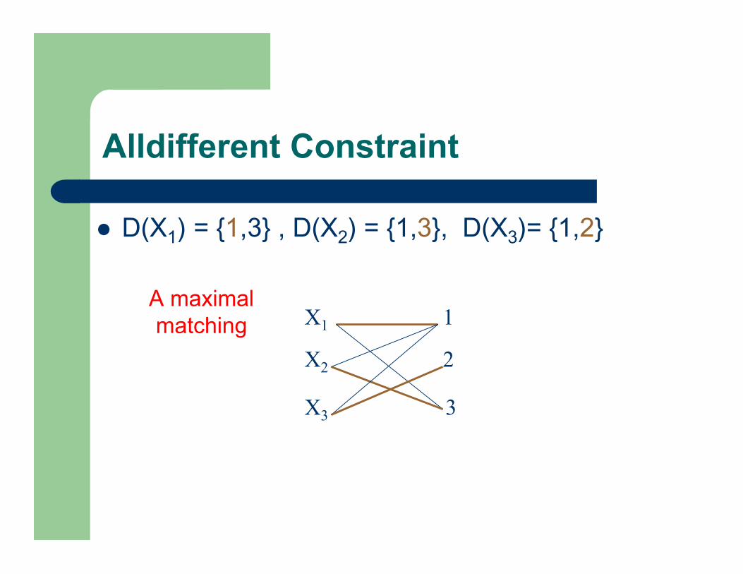
Matching: set of edges with no two edges having a nodein common.
Maximal matching: largest possible matching.
Alldifferent Constraint
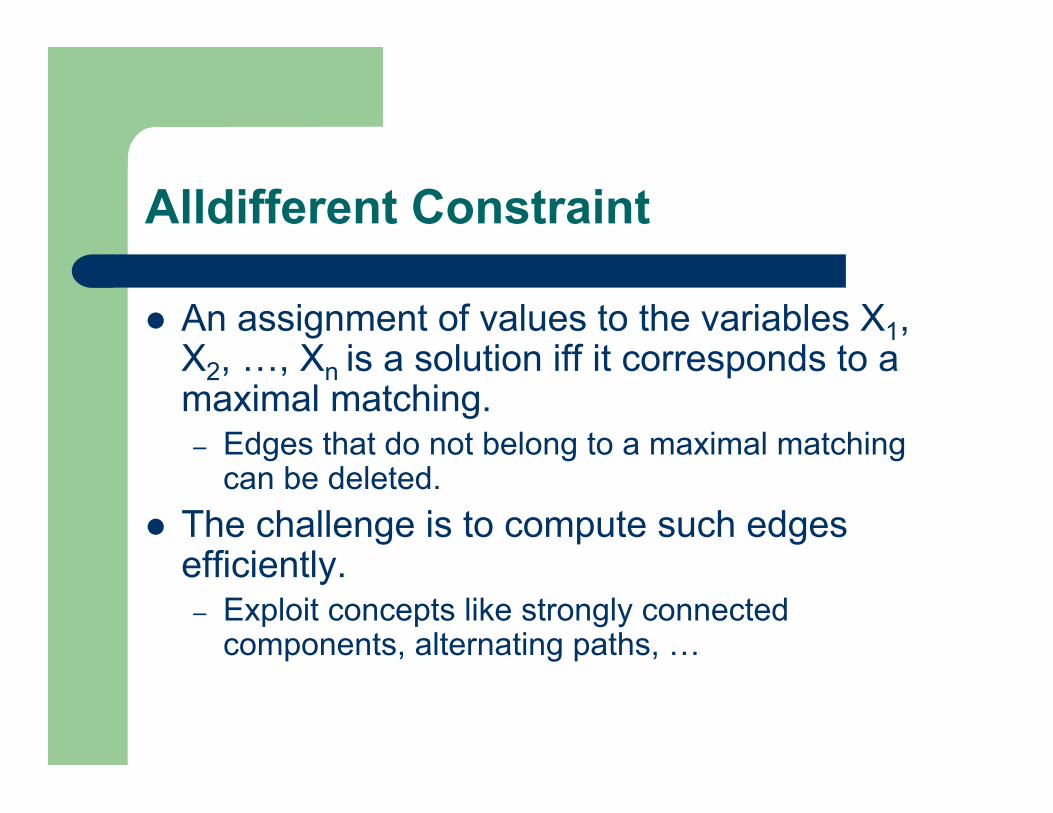
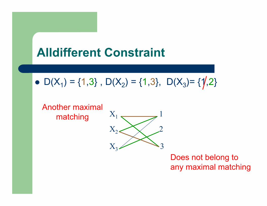
An assignment of values to the variables X1,X2, …, Xn is a solution iff it corresponds to amaximal matching.– Edges that do not belong to a maximal matching
can be deleted.
The challenge is to compute such edgesefficiently.– Exploit concepts like strongly connected
components, alternating paths, …
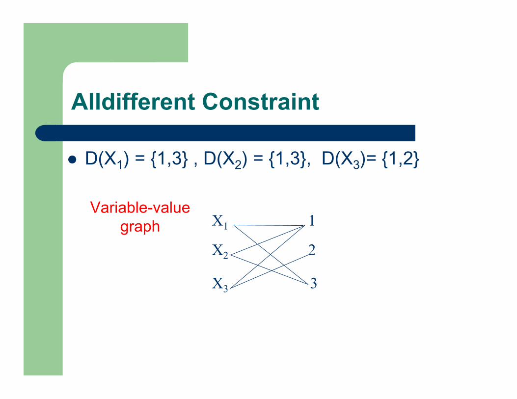
Alldifferent Constraint
D(X1) = {1,3} , D(X2) = {1,3}, D(X3)= {1,2}
X1
X2
X3
1
2
3
Variable-valuegraph
Alldifferent Constraint
D(X1) = {1,3} , D(X2) = {1,3}, D(X3)= {1,2}
X1
X2
X3
1
2
3
A maximalmatching
Alldifferent Constraint
D(X1) = {1,3} , D(X2) = {1,3}, D(X3)= {1,2}
X1
X2
X3
1
2
3
Another maximalmatching
Does not belong toany maximal matching
Other Examples of Global Constraints
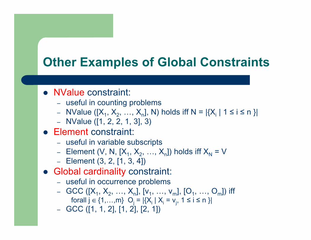
NValue constraint:– useful in counting problems– NValue ([X1, X2, …, Xn], N) holds iff N = |{Xi | 1 ≤ i ≤ n }|– NValue ([1, 2, 2, 1, 3], 3)
Element constraint:– useful in variable subscripts– Element (V, N, [X1, X2, …, Xn]) holds iff XN = V– Element (3, 2, [1, 3, 4])
Global cardinality constraint:– useful in occurrence problems– GCC ([X1, X2, …, Xn], [v1, …, vm], [O1, …, Om]) iff
forall j ∈ {1,…,m} Oj = |{Xi | Xi = vj, 1 ≤ i ≤ n }|– GCC ([1, 1, 2], [1, 2], [2, 1])
Other Examples of Global Constraints
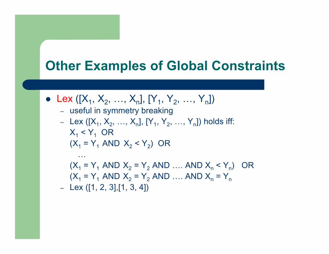
Lex ([X1, X2, …, Xn], [Y1, Y2, …, Yn])– useful in symmetry breaking– Lex ([X1, X2, …, Xn], [Y1, Y2, …, Yn]) holds iff: X1 < Y1 OR (X1 = Y1 AND X2 < Y2) OR
… (X1 = Y1 AND X2 = Y2 AND …. AND Xn < Yn) OR (X1 = Y1 AND X2 = Y2 AND …. AND Xn = Yn
– Lex ([1, 2, 3],[1, 3, 4])
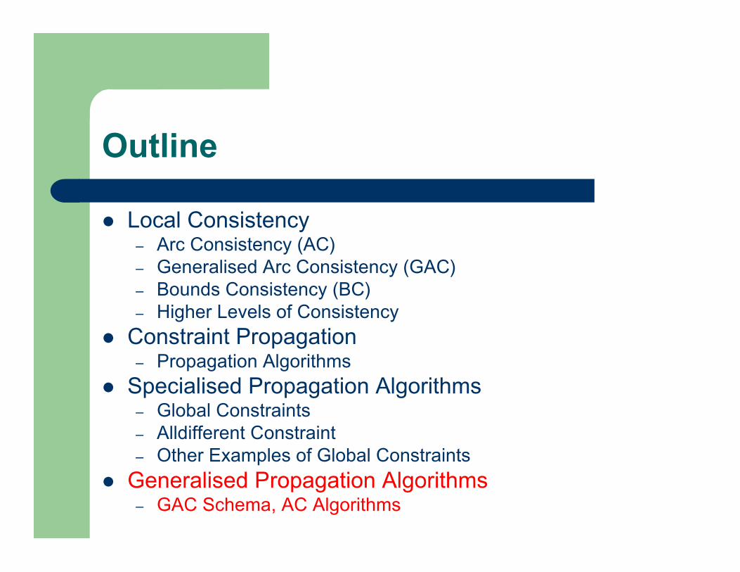
Outline
Local Consistency– Arc Consistency (AC)– Generalised Arc Consistency (GAC)– Bounds Consistency (BC)– Higher Levels of Consistency
Constraint Propagation– Propagation Algorithms
Specialised Propagation Algorithms– Global Constraints– Alldifferent Constraint– Other Examples of Global Constraints
Generalised Propagation Algorithms– GAC Schema, AC Algorithms
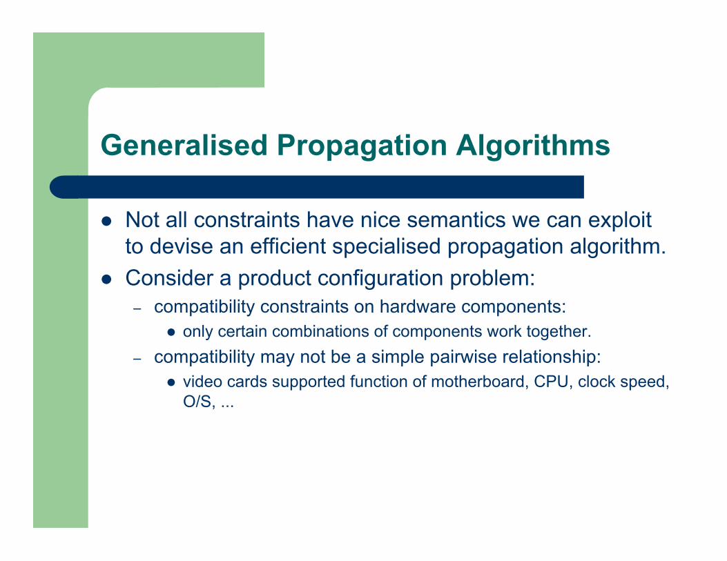
Generalised Propagation Algorithms
Not all constraints have nice semantics we can exploitto devise an efficient specialised propagation algorithm.
Consider a product configuration problem:– compatibility constraints on hardware components:
only certain combinations of components work together.
– compatibility may not be a simple pairwise relationship: video cards supported function of motherboard, CPU, clock speed,
O/S, ...

Production Configuration Problem
5-ary constraint:– Compatible (motherboard345, intelCPU,
2GHz, 1GBRam, 80GBdrive).)– Compatible (motherboard346, intelCPU,
3GHz, 2GBRam, 100GBdrive).– Compatible (motherboard346, amdCPU,
2GHz, 2GBRam, 100GBdrive).– …
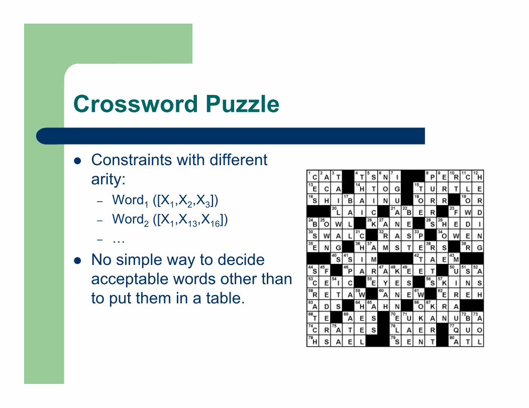
Crossword Puzzle
Constraints with differentarity:
– Word1 ([X1,X2,X3])
– Word2 ([X1,X13,X16])
– …
No simple way to decideacceptable words other thanto put them in a table.
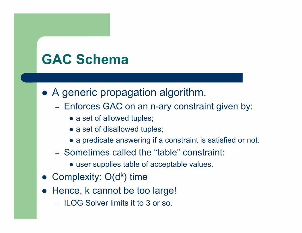
GAC Schema
A generic propagation algorithm.– Enforces GAC on an n-ary constraint given by:
a set of allowed tuples;
a set of disallowed tuples;
a predicate answering if a constraint is satisfied or not.
– Sometimes called the “table” constraint: user supplies table of acceptable values.
Complexity: O(dk) time
Hence, k cannot be too large!– ILOG Solver limits it to 3 or so.
Arc Consistency Algorithms
Generic AC algorithms with differentcomplexities and advantages:
– AC3
– AC4
– AC6
– AC2001
– …

PART III: Some Useful Pointersabout CP
(Incomplete) List of Advanced Topics
Modelling Global constraints,
propagation algorithms Search algorithms Heuristics Symmetry breaking Optimisation Local search Soft constraints, preferences Temporal constraints Quantified constraints Continuous constraints
Planning and scheduling SAT Complexity and tractability Uncertainty Robustness Structured domains Randomisation Hybrid systems Applications Constraint systems No good learning Explanations Visualisation
Literature
Books– My PhD dissertation
– Handbook of Constraint ProgrammingF. Rossi, P. van Beek, T. Walsh (eds), Elsevier Science, 2006.
Some online chapters:
Chapter 1 - Introduction
Chapter 3 - Constraint Propagation
Chapter 6 - Global Constraints
Chapter 10 - Symmetry in CP
Chapter 11 - Modelling
Literature
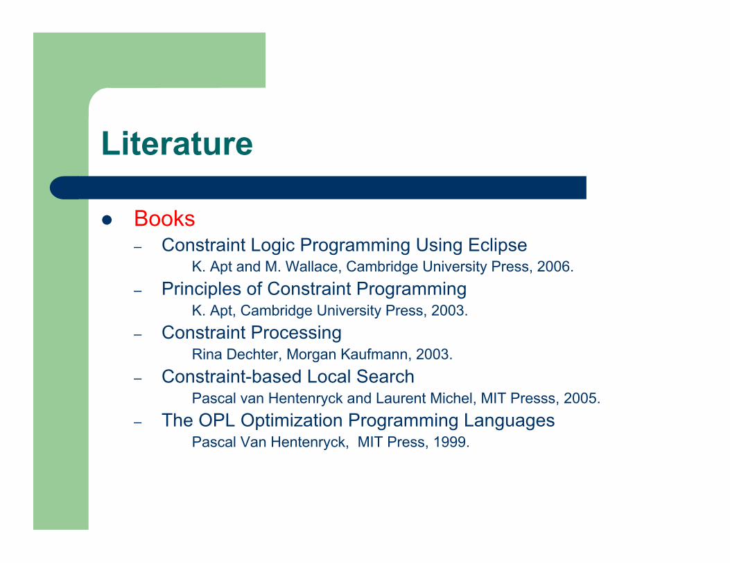
Books– Constraint Logic Programming Using Eclipse
K. Apt and M. Wallace, Cambridge University Press, 2006.
– Principles of Constraint ProgrammingK. Apt, Cambridge University Press, 2003.
– Constraint ProcessingRina Dechter, Morgan Kaufmann, 2003.
– Constraint-based Local SearchPascal van Hentenryck and Laurent Michel, MIT Presss, 2005.
– The OPL Optimization Programming LanguagesPascal Van Hentenryck, MIT Press, 1999.
Literature
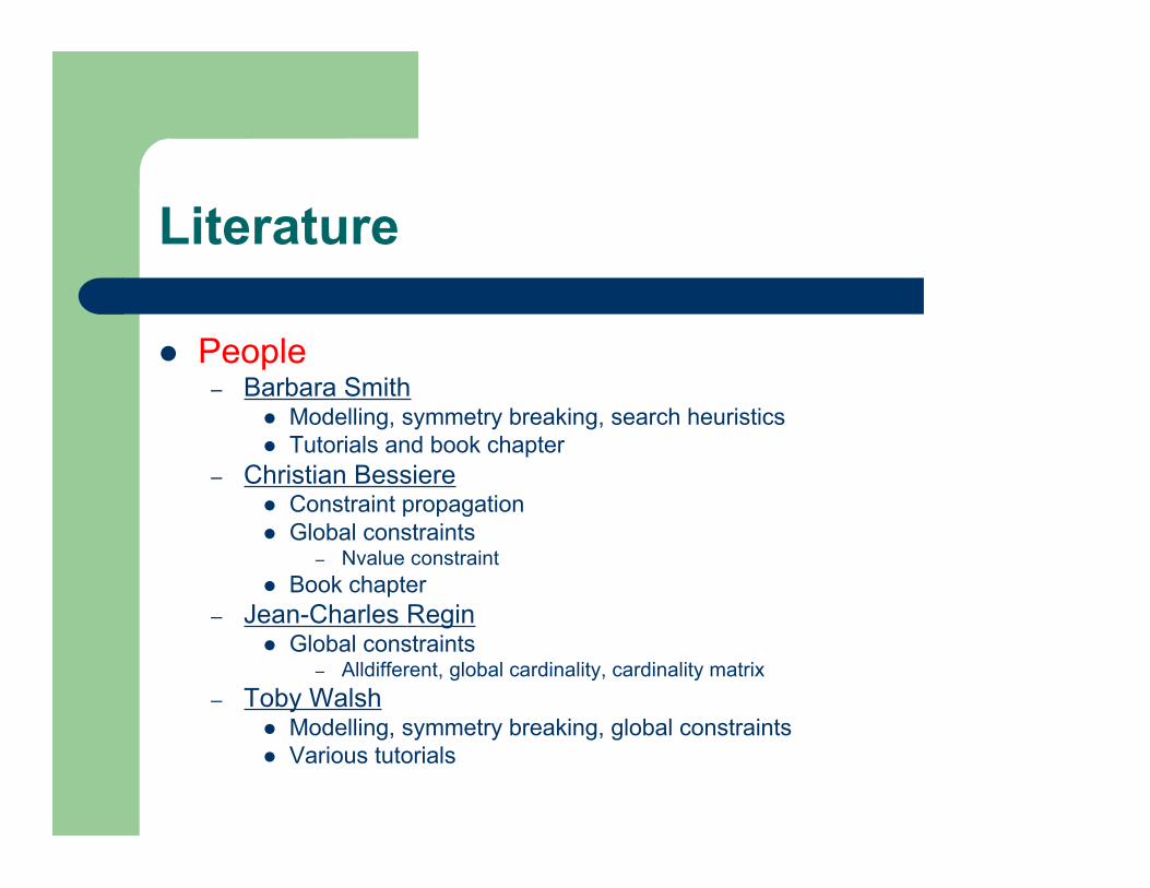
People– Barbara Smith
Modelling, symmetry breaking, search heuristics Tutorials and book chapter
– Christian Bessiere Constraint propagation Global constraints
– Nvalue constraint Book chapter
– Jean-Charles Regin Global constraints
– Alldifferent, global cardinality, cardinality matrix
– Toby Walsh Modelling, symmetry breaking, global constraints Various tutorials
Literature
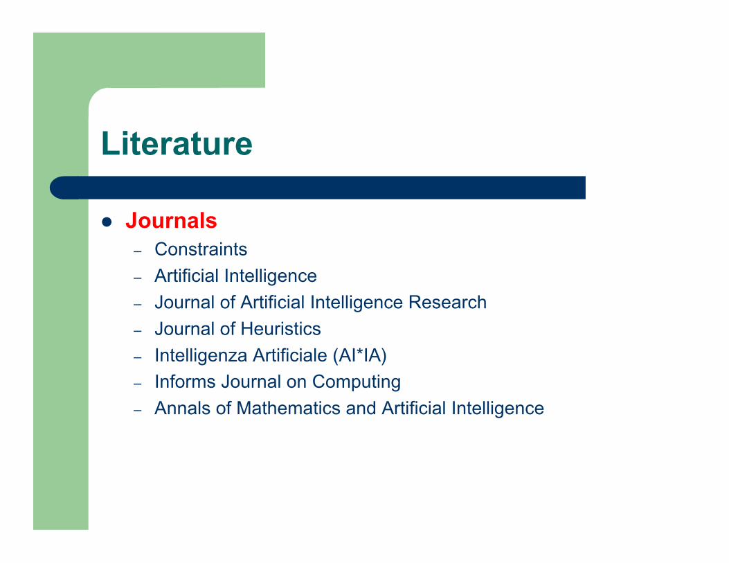
Journals– Constraints
– Artificial Intelligence
– Journal of Artificial Intelligence Research
– Journal of Heuristics
– Intelligenza Artificiale (AI*IA)
– Informs Journal on Computing
– Annals of Mathematics and Artificial Intelligence
Literature
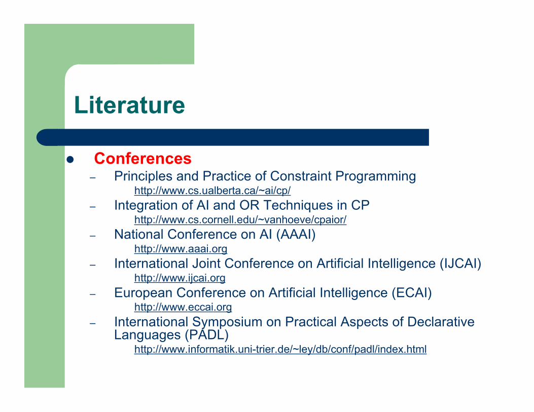
Conferences– Principles and Practice of Constraint Programming
http://www.cs.ualberta.ca/~ai/cp/
– Integration of AI and OR Techniques in CPhttp://www.cs.cornell.edu/~vanhoeve/cpaior/
– National Conference on AI (AAAI)http://www.aaai.org
– International Joint Conference on Artificial Intelligence (IJCAI)http://www.ijcai.org
– European Conference on Artificial Intelligence (ECAI)http://www.eccai.org
– International Symposium on Practical Aspects of DeclarativeLanguages (PADL)
http://www.informatik.uni-trier.de/~ley/db/conf/padl/index.html
Literature
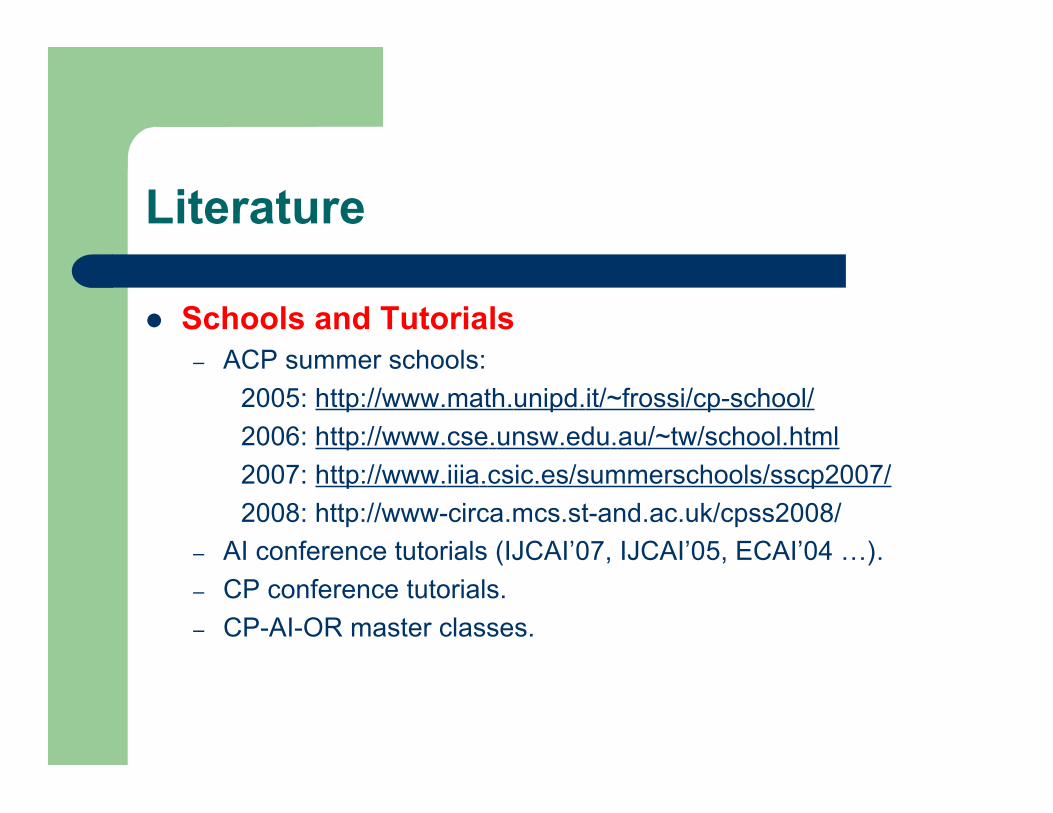
Schools and Tutorials– ACP summer schools:
2005: http://www.math.unipd.it/~frossi/cp-school/
2006: http://www.cse.unsw.edu.au/~tw/school.html
2007: http://www.iiia.csic.es/summerschools/sscp2007/
2008: http://www-circa.mcs.st-and.ac.uk/cpss2008/
– AI conference tutorials (IJCAI’07, IJCAI’05, ECAI’04 …).
– CP conference tutorials.
– CP-AI-OR master classes.
Literature
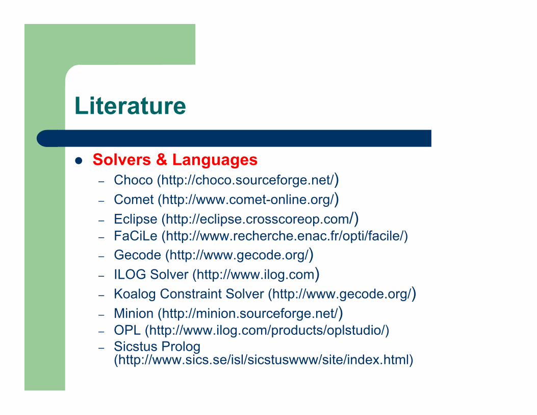
Solvers & Languages– Choco (http://choco.sourceforge.net/)– Comet (http://www.comet-online.org/)– Eclipse (http://eclipse.crosscoreop.com/)– FaCiLe (http://www.recherche.enac.fr/opti/facile/)
– Gecode (http://www.gecode.org/)– ILOG Solver (http://www.ilog.com)– Koalog Constraint Solver (http://www.gecode.org/)– Minion (http://minion.sourceforge.net/)– OPL (http://www.ilog.com/products/oplstudio/)– Sicstus Prolog
(http://www.sics.se/isl/sicstuswww/site/index.html)