Mathematical Preliminaries - faculty.missouri.edufaculty.missouri.edu/~hedlunda/teaching/2013b/3 - mathprelims.pdf · Mathematical Preliminaries Economics 3307 - Intermediate Macroeconomics

Mathematical Preliminaries

Economics 3307 - Intermediate Macroeconomics

Aaron Hedlund

Baylor University

Fall 2013

Econ 3307 (Baylor University) Mathematical Preliminaries Fall 2013 1 / 25

Outline

I: Sequences and Series

II: Continuity and Differentiation

III: Optimization and Comparative Statics

IV: Basic Probability and Statistics


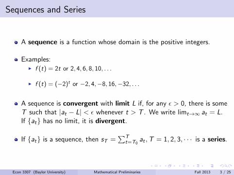
Sequences and Series

A sequence is a function whose domain is the positive integers.

Examples:I f (t) = 2t or 2, 4, 6, 8, 10, . . .

I f (t) = (−2)t or −2, 4,−8, 16,−32, . . .

A sequence is convergent with limit L if, for any ε > 0, there is someT such that |at − L| < ε whenever t > T . We write limt→∞ at = L.If at has no limit, it is divergent.

If at is a sequence, then sT =∑T

t=T0at ,T = 1, 2, 3, · · · is a series.



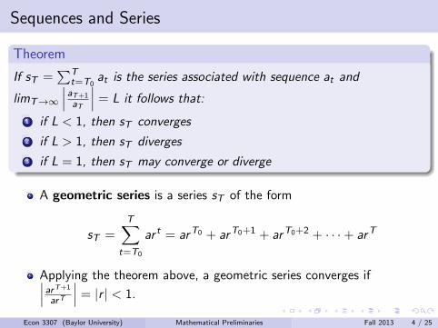
Theorem

If sT =∑T

t=T0at is the series associated with sequence at and

limT→∞

∣∣∣aT+1

aT

∣∣∣ = L it follows that:

1 if L < 1, then sT converges

2 if L > 1, then sT diverges

3 if L = 1, then sT may converge or diverge

A geometric series is a series sT of the form

sT =T∑

t=T0

ar t = arT0 + arT0+1 + arT0+2 + · · ·+ arT

Applying the theorem above, a geometric series converges if∣∣∣arT+1

arT

∣∣∣ = |r | < 1.



The partial sum of a geometric series can be written explicitly as

T∑t=T0

ar t =arT0(1− rT−T0+1)

1− r

Taking the limit when r < 1, we get

limT→∞

T∑t=T0

ar t =arT0

1− r

The present value PV of a stream of payments πtTt=1, discountedat rate r , is given by

PV =T∑t=1

πt(1 + r)t−1


Continuity and Differentiation

A function f : (a, b)→ R is continuous at x0 ∈ (a, b) if, for anyε > 0, there exists δ > 0 such that |f (x)− f (x0)| < ε whenever|x − x0| < δ.

We say that f (x) is differentiable at x ∈ (a, b) if the limit

f ′(x) = lim∆x→0

f (x + ∆x)− f (x)

∆x

exists and is finite. The derivative of y = f (x) can also be written asdydx or df

dx .

A function is continuously differentiable on a set S if it isdifferentiable and its derivative is continuous on S .


Differentiation Rules

1 f (x) = c ⇒ f ′(x) = 0.

2 f (x) = xn ⇒ f ′(x) = nxn−1.

3 g(x) = cf (x)⇒ g ′(x) = cf ′(x).

4 h(x) = f (x)± g(x)⇒ h′(x) = f ′(x)± g ′(x).

5 h(x) = f (x)g(x)⇒ h′(x) = f ′(x)g(x) + f (x)g ′(x).

6 h(x) = f (x)g(x) ⇒ h′(x) = g(x)f ′(x)−f (x)g ′(x)

[g(x)]2 .

7 h(x) = f (g(x))⇒ h′(x) = f ′(g(x))g ′(x), or dhdx = df

dx |g(x)dgdx .

8 h(x) = f −1(x)⇒ h′(x) = 1f ′(f −1(x))

, or dhdx = 1

dfdx|f−1(x)

.


Partial Differentiation

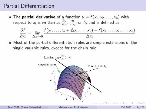
The partial derivative of a function y = f (x1, x2, . . . , xn) withrespect to xi is written as ∂y

∂xi, ∂f∂xi

, or fi , and is defined as

∂f

∂xi= lim

∆xi→0

f (x1, . . . , xi + ∆xi , . . . , xn)− f (x1, . . . , xi , . . . , xn)

∆xi

Most of the partial differentiation rules are simple extensions of thesingle variable rules, except for the chain rule.


Multivariable Chain Rule and Total Differentiation

Chain rule: Let y = f (u1, u2, . . . , um) and ui = gi (x1, x2, . . . , xn) forall i = 1, 2, ...,m. Denote x = (x1, . . . , xn) and defineh(x) = f (g1(x), . . . , gm(x)). Then

∂h

∂xj=

∂f

∂u1

∂g1

∂xj+∂f

∂u2

∂g2

∂xj+· · ·+ ∂f

∂um

∂gm∂xj

=m∑i=1

∂f

∂ui

∣∣∣∣ui=gi (x)

∂gi∂xj

, i.e.

∂y

∂xj=

∂y

∂u1

∂u1

∂xj+∂y

∂u2

∂u2

∂xj+ · · ·+ ∂y

∂um

∂um∂xj

=m∑i=1

∂y

∂ui

∣∣∣∣ui=gi (x)

∂ui∂xj

The total differential of a function f (x) is

df =n∑

i=1

∂f

∂xidxi


Second-Order Partial Derivatives

The second-order partial derivative of f (x) with respect to xi andthen xj is

fij =∂fi (x)

∂xj

Theorem (Young’s Theorem)

If f (x) has continuous first-order and second-order partial derivatives, theorder of differentiation in computing the cross-partial is irrelevant, i.e.fij = fji .


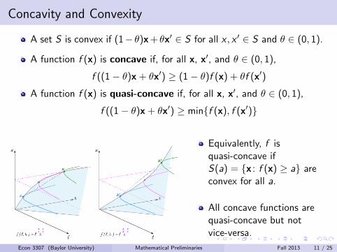
Concavity and Convexity

A set S is convex if (1− θ)x + θx′ ∈ S for all x , x ′ ∈ S and θ ∈ (0, 1).

A function f (x) is concave if, for all x, x′, and θ ∈ (0, 1),

f ((1− θ)x + θx′) ≥ (1− θ)f (x) + θf (x′)

A function f (x) is quasi-concave if, for all x, x′, and θ ∈ (0, 1),

f ((1− θ)x + θx′) ≥ minf (x), f (x′)

Equivalently, f isquasi-concave ifS(a) = x : f (x) ≥ a areconvex for all a.

All concave functions arequasi-concave but notvice-versa.


Concavity and Differentiability

Univariate functions: Let f (x) be twice continuously differentiable.I If f is concave, then f

′′ ≤ 0.

Bivariate functions: Let f (x1, x2) be twice continuously differentiable.I If f is concave, then f11 ≤ 0 and f11f22 − (f12)2 ≥ 0.

I If f (x1, x2) is quasi-concave, then f11f2

2 − 2f1f2f12 + f22f2

1 < 0.


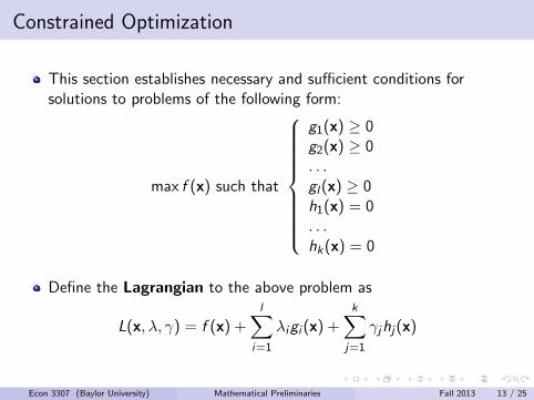
Constrained Optimization

This section establishes necessary and sufficient conditions forsolutions to problems of the following form:

max f (x) such that

g1(x) ≥ 0g2(x) ≥ 0. . .gl(x) ≥ 0h1(x) = 0. . .hk(x) = 0

Define the Lagrangian to the above problem as

L(x, λ, γ) = f (x) +l∑

i=1

λigi (x) +k∑

j=1

γjhj(x)


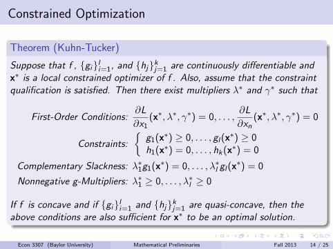
Constrained Optimization

Theorem (Kuhn-Tucker)

Suppose that f , gili=1, and hjkj=1 are continuously differentiable andx∗ is a local constrained optimizer of f . Also, assume that the constraintqualification is satisfied. Then there exist multipliers λ∗ and γ∗ such that

First-Order Conditions:∂L

∂x1(x∗, λ∗, γ∗) = 0, . . . ,

∂L

∂xn(x∗, λ∗, γ∗) = 0

Constraints:

g1(x∗) ≥ 0, . . . , gl(x∗) ≥ 0h1(x∗) = 0, . . . , hk(x∗) = 0

Complementary Slackness: λ∗1g1(x∗) = 0, . . . , λ∗l gl(x∗) = 0

Nonnegative g-Multipliers: λ∗1 ≥ 0, . . . , λ∗l ≥ 0

If f is concave and if gili=1 and hjkj=1 are quasi-concave, then theabove conditions are also sufficient for x∗ to be an optimal solution.


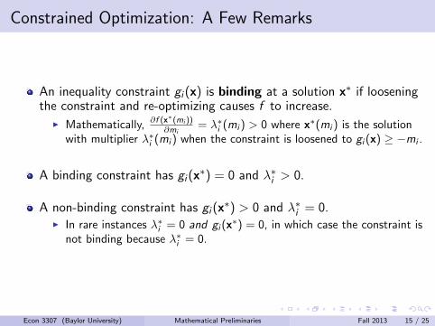
Constrained Optimization: A Few Remarks

An inequality constraint gi (x) is binding at a solution x∗ if looseningthe constraint and re-optimizing causes f to increase.

I Mathematically, ∂f (x∗(mi ))∂mi

= λ∗i (mi ) > 0 where x∗(mi ) is the solutionwith multiplier λ∗i (mi ) when the constraint is loosened to gi (x) ≥ −mi .

A binding constraint has gi (x∗) = 0 and λ∗i > 0.

A non-binding constraint has gi (x∗) > 0 and λ∗i = 0.I In rare instances λ∗i = 0 and gi (x∗) = 0, in which case the constraint is

not binding because λ∗i = 0.


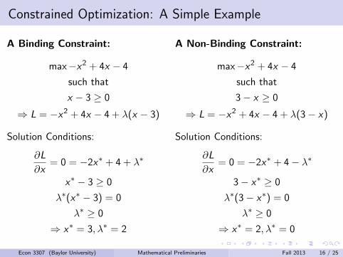
Constrained Optimization: A Simple Example

A Binding Constraint:

max−x2 + 4x − 4

such that

x − 3 ≥ 0

⇒ L = −x2 + 4x − 4 + λ(x − 3)

Solution Conditions:

∂L

∂x= 0 = −2x∗ + 4 + λ∗

x∗ − 3 ≥ 0

λ∗(x∗ − 3) = 0

λ∗ ≥ 0

⇒ x∗ = 3, λ∗ = 2

A Non-Binding Constraint:

max−x2 + 4x − 4

such that

3− x ≥ 0

⇒ L = −x2 + 4x − 4 + λ(3− x)

Solution Conditions:

∂L

∂x= 0 = −2x∗ + 4− λ∗

3− x∗ ≥ 0

λ∗(3− x∗) = 0

λ∗ ≥ 0

⇒ x∗ = 2, λ∗ = 0


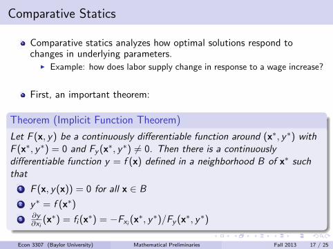
Comparative Statics

Comparative statics analyzes how optimal solutions respond tochanges in underlying parameters.

I Example: how does labor supply change in response to a wage increase?

First, an important theorem:

Theorem (Implicit Function Theorem)

Let F (x, y) be a continuously differentiable function around (x∗, y∗) withF (x∗, y∗) = 0 and Fy (x∗, y∗) 6= 0. Then there is a continuouslydifferentiable function y = f (x) defined in a neighborhood B of x∗ suchthat

1 F (x, y(x)) = 0 for all x ∈ B

2 y∗ = f (x∗)

3∂y∂xi

(x∗) = fi (x∗) = −Fxi (x∗, y∗)/Fy (x∗, y∗)


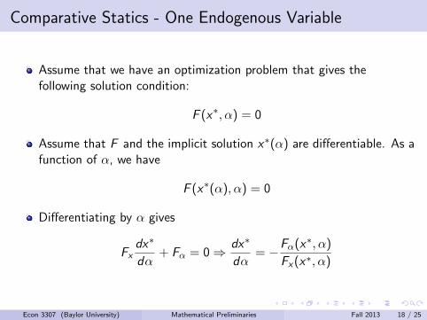
Comparative Statics - One Endogenous Variable

Assume that we have an optimization problem that gives thefollowing solution condition:

F (x∗, α) = 0

Assume that F and the implicit solution x∗(α) are differentiable. As afunction of α, we have

F (x∗(α), α) = 0

Differentiating by α gives

Fxdx∗

dα+ Fα = 0⇒ dx∗

dα= −Fα(x∗, α)

Fx(x∗, α)


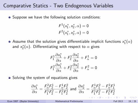
Comparative Statics - Two Endogenous Variables

Suppose we have the following solution conditions:

F 1(x∗1 , x∗2 , α) = 0

F 2(x∗1 , x∗2 , α) = 0

Assume that the solution gives differentiable implicit functions x∗1 (α)and x∗2 (α). Differentiating with respect to α gives

F 11

∂x∗1∂α

+ F 12

∂x∗2∂α

+ F 1α = 0

F 21

∂x∗1∂α

+ F 22

∂x∗2∂α

+ F 2α = 0

Solving the system of equations gives

∂x∗1∂α

=F 2αF

12 − F 1

αF22

F 11 F

22 − F 2

1 F12

and∂x∗2∂α

=F 1αF

21 − F 2

αF11

F 11 F

22 − F 2

1 F12


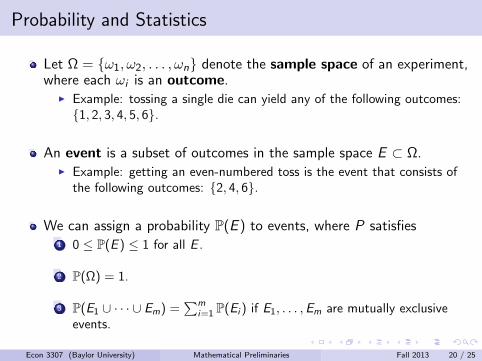
Probability and Statistics

Let Ω = ω1, ω2, . . . , ωn denote the sample space of an experiment,where each ωi is an outcome.

I Example: tossing a single die can yield any of the following outcomes:1, 2, 3, 4, 5, 6.

An event is a subset of outcomes in the sample space E ⊂ Ω.I Example: getting an even-numbered toss is the event that consists of

the following outcomes: 2, 4, 6.

We can assign a probability P(E ) to events, where P satisfies1 0 ≤ P(E ) ≤ 1 for all E .

2 P(Ω) = 1.

3 P(E1 ∪ · · · ∪ Em) =∑m

i=1 P(Ei ) if E1, . . . ,Em are mutually exclusiveevents.


Conditional Probability and Independence

The conditional probability of E2 given E1 is the probability that E2

will occur given that E1 has occurred. It is represented by

P(E2|E1) =P(E1 ∩ E2)

P(E1)

Events E1 and E2 are independent if P(E2|E1) = P(E2), orequivalently, if P(E1 ∩ E2) = P(E1)P(E2).

In applications it is useful to know Bayes’ rule:

P(E |F ) =P(E ∩ F )

P(F )=

P(F |E )P(E )

P(F |E )P(E ) + P(F |E c)P(E c)


Random Variables and Expectations

A random variable X is a function defined on a sample space,X : Ω→ R.

I Example: Ω = Heads, Tails, X (Heads) = 0, X (Tails) = 1.

The expected value or mean of a random variable X is

E(X ) =n∑

i=1

xiP(ω : X (ω) = xi )

where X takes on values x1, . . . , xn. Let P(xi ) = P(ω : X (ω) = xi ).I Above example: E(X ) = 0 · 0.5 + 1 · 0.5 = 0.5.

We often write µX instead of E(X ).


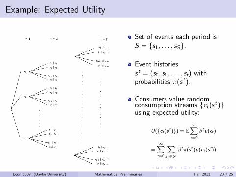
Example: Expected Utility

Set of events each period isS = s1, . . . , sS.

Event historiesst = (s0, s1, . . . , st) withprobabilities π(st).

Consumers value randomconsumption streams ct(st)using expected utility:

U(ct(st)) = E∞∑t=0

βtu(ct)

=∞∑t=0

∑st∈St

βtπ(st)u(ct(st))


Variance, Covariance, and Correlation

The variance of a random variable is

Var(X ) = E[(X − µX )2] =n∑

i=1

(xi − µX )2P(xi )

The covariance of two random variables X and Y is

Cov(X ,Y ) = E[(X−µX )(Y −µY )] =n∑

i=1

(xi − µX )(yi − µY )P(xi , yi )

The correlation between X and Y is Corr(X ,Y ) = Cov(X ,Y )SD(X )SD(Y ) ,

where SD(X ) =√Var(X ) is the standard deviation of X .


Sample Statistics

When confronting actual data, the underlying probabilities are notreadily observable, forcing us to compute sample statistics.

Suppose we have data (x1, y1), (x2, y2), . . . , (xn, yn).

The sample mean and variance of X are X = 1n

∑ni=1 xi and

Var(X ) = 1n−1

∑ni=1 (xi − X )2.

The sample covariance between X and Y isCov(X ,Y ) = 1

n−1

∑ni=1 (xi − X )(yi − Y ).


Documents

Mathematical Preliminaries - faculty.missouri.edufaculty.missouri.edu/~hedlunda/teaching/2013b/3 - mathprelims.pdf · Mathematical Preliminaries Economics 3307 - Intermediate Macroeconomics