Economics 310

Lecture 24Univariate Time Series

Concepts to be Discussed Time Series Stationarity Spurious regression Trends

Plot of Economic Levels Data

PPI, M1, Employment

0.000

20.000

40.000

60.000

80.000

100.000

120.000

140.000

160.000

1980

1980

1981

1982

1982

1983

1984

1984

1985

1986

1986

1987

1988

1988

1989

1990

1990

1991

1992

1992

1993

1994

1994

1995

1996

1996

1997

1998

1998

1999

2000

Date

employ*

M1*

PPIACO

Plot of Rate DataExchange Rate & Interest Rate

-30

-20

-10

0

10

20

30

40

50

1976

1976

1977

1978

1979

1980

1981

1981

1982

1983

1984

1985

1986

1986

1987

1988

1989

1990

1991

1991

1992

1993

1994

1995

1996

1996

1997

1998

1999

2000

Date

Pe

rce

nt

TWEXMMTH

BA6M

Stationary Stochastic Process Stochastic Random Process Realization A Stochastic process is said to be stationary if

its mean and variance are constant over time and the value of covariance between two time periods depends only on the distance or lag between the two time periods and not on the actual time at which the covariance is computed.

A time series is not stationary in the sense just define if conditions are violated. It is called a nonstationary time series.

Stationary Stochastic Process

ktallforYYEianceCo

tallforYEYiance

tallforYEMean

tystationariforConditions

kttk

tt

t

&)])([(:var

)()var(:var

)(:22

Test for Stationarity: Correlogram

mcorrelogra

sample theisation autocorrel sample theofplot

ˆ

ˆˆ

ˆ

ˆ

function.ation autocorrel sample thecomputecan We

mcorrelogra polulation thegives thisofGraph

var

var

(ACF)Function ation Autocorrel

0k

2

0

k

0k

The

n

YY

n

YYYY

iance

klagatianceCo

k

t

ktt

k

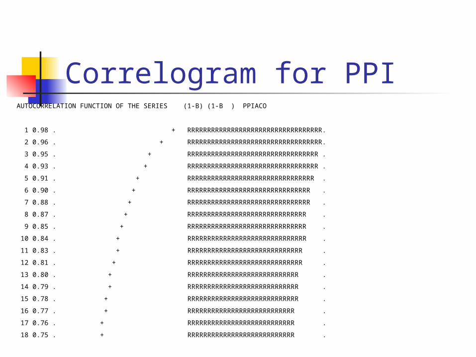
Correlogram for PPIAUTOCORRELATION FUNCTION OF THE SERIES (1-B) (1-B ) PPIACO

1 0.98 . + RRRRRRRRRRRRRRRRRRRRRRRRRRRRRRRRRR.

2 0.96 . + RRRRRRRRRRRRRRRRRRRRRRRRRRRRRRRRRR.

3 0.95 . + RRRRRRRRRRRRRRRRRRRRRRRRRRRRRRRRR .

4 0.93 . + RRRRRRRRRRRRRRRRRRRRRRRRRRRRRRRRR .

5 0.91 . + RRRRRRRRRRRRRRRRRRRRRRRRRRRRRRRR .

6 0.90 . + RRRRRRRRRRRRRRRRRRRRRRRRRRRRRRR .

7 0.88 . + RRRRRRRRRRRRRRRRRRRRRRRRRRRRRRR .

8 0.87 . + RRRRRRRRRRRRRRRRRRRRRRRRRRRRRR .

9 0.85 . + RRRRRRRRRRRRRRRRRRRRRRRRRRRRRR .

10 0.84 . + RRRRRRRRRRRRRRRRRRRRRRRRRRRRRR .

11 0.83 . + RRRRRRRRRRRRRRRRRRRRRRRRRRRRR .

12 0.81 . + RRRRRRRRRRRRRRRRRRRRRRRRRRRRR .

13 0.80 . + RRRRRRRRRRRRRRRRRRRRRRRRRRRR .

14 0.79 . + RRRRRRRRRRRRRRRRRRRRRRRRRRRR .

15 0.78 . + RRRRRRRRRRRRRRRRRRRRRRRRRRRR .

16 0.77 . + RRRRRRRRRRRRRRRRRRRRRRRRRRR .

17 0.76 . + RRRRRRRRRRRRRRRRRRRRRRRRRRR .

18 0.75 . + RRRRRRRRRRRRRRRRRRRRRRRRRRR .

Correlogram M1AUTOCORRELATION FUNCTION OF THE SERIES (1-B) (1-B ) M1

1 0.99 . + RRRRRRRRRRRRRRRRRRRRRRRRRRRRRRRRRRR

2 0.98 . + RRRRRRRRRRRRRRRRRRRRRRRRRRRRRRRRRR.

3 0.97 . + RRRRRRRRRRRRRRRRRRRRRRRRRRRRRRRRRR.

4 0.96 . + RRRRRRRRRRRRRRRRRRRRRRRRRRRRRRRRRR.

5 0.95 . + RRRRRRRRRRRRRRRRRRRRRRRRRRRRRRRRR .

6 0.94 . + RRRRRRRRRRRRRRRRRRRRRRRRRRRRRRRRR .

7 0.93 . + RRRRRRRRRRRRRRRRRRRRRRRRRRRRRRRRR .

8 0.92 . + RRRRRRRRRRRRRRRRRRRRRRRRRRRRRRRR .

9 0.91 . + RRRRRRRRRRRRRRRRRRRRRRRRRRRRRRRR .

10 0.90 . + RRRRRRRRRRRRRRRRRRRRRRRRRRRRRRRR .

11 0.89 . + RRRRRRRRRRRRRRRRRRRRRRRRRRRRRRR .

12 0.88 . + RRRRRRRRRRRRRRRRRRRRRRRRRRRRRRR .

13 0.87 . + RRRRRRRRRRRRRRRRRRRRRRRRRRRRRRR .

14 0.86 . + RRRRRRRRRRRRRRRRRRRRRRRRRRRRRR .

15 0.85 . + RRRRRRRRRRRRRRRRRRRRRRRRRRRRRR .

16 0.84 . + RRRRRRRRRRRRRRRRRRRRRRRRRRRRR .

17 0.83 . + RRRRRRRRRRRRRRRRRRRRRRRRRRRRR .

18 0.81 . + RRRRRRRRRRRRRRRRRRRRRRRRRRRRR .

Testing autocorrelation coefficients If data is white noise, the sample

autocorrelation coefficient is normally distributed with mean zero and variance ~ 1/n

For our levels data sd=0.064, and 5% test cut off is 0.126

For our rate data, sd=0.059, and 5% test cut off is 0.115

Testing Autocorrelation coefficients

2m

1k

2k

2m

1k

2k

~ˆ

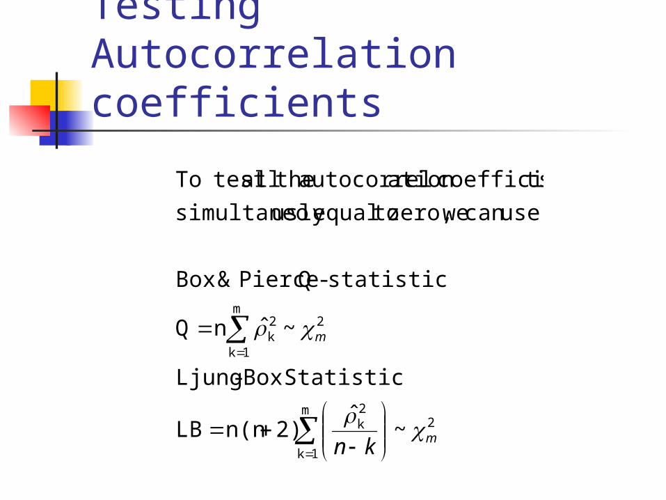
2)n(nLB

StatisticBox -Ljung

~ˆnQ

statistic-Q Pierce &Box

usecan wezero, toequalusly simultaneo

tscoefficienation autocorrel theall test To

m

m

kn

Ljung-Box test for PPISERIES (1-B) (1-B ) PPIACO

NET NUMBER OF OBSERVATIONS = 242

MEAN= 112.01 VARIANCE= 129.36 STANDARD DEV.= 11.374

LAGS AUTOCORRELATIONS STD ERR

1 -12 0.98 0.96 0.95 0.93 0.91 0.90 0.88 0.87 0.85 0.84 0.83 0.81 0.06

13 -18 0.80 0.79 0.78 0.77 0.76 0.75 0.29

MODIFIED BOX-PIERCE (LJUNG-BOX-PIERCE) STATISTICS (CHI-SQUARE)

LAG Q DF P-VALUE LAG Q DF P-VALUE

1 236.25 1 .000 10 2060.22 10 .000

2 465.31 2 .000 11 2234.89 11 .000

3 687.34 3 .000 12 2405.13 12 .000

4 902.18 4 .000 13 2571.38 13 .000

5 1110.17 5 .000 14 2733.79 14 .000

6 1311.32 6 .000 15 2892.87 15 .000

7 1506.47 7 .000 16 3048.83 16 .000

8 1696.30 8 .000 17 3201.65 17 .000

9 1880.78 9 .000 18 3351.37 18 .000

Unit Root Test for Stationarity

.0

)1(

mod,

..

,1

Y ,regression run the weIf

situation.arity nonstationA problem.root unit

thehave we1, is Y oft coefficien fact thein

mod

11

1t

1-t

1

testWe

YYY

eltheestimatesoneFrequently

walkrandomaisseriesTheproblemrootunit

ahavewefromdifferenttestnotdoesand

Y

If

noisewhiteis

YY

eltheConsider

ttttt

tt

t

ttt

Results of our test If a time series is differenced once

and the differenced series is stationary, we say that the original (random walk) is integrated of order 1, and is denoted I(1).

If the original series has to be differenced twice before it is stationary, we say it is integrated of order 2, I(2).

Testing for unit root In testing for a unit root, we can

not use the traditional t values for the test.

We used revised critical values provided by Dickey and Fuller.

We call the test the Dickey-Fuller test for unit roots.

Dickey-Fuller Test

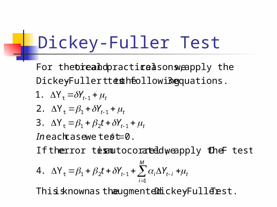
Test.Fuller -Dickey augmented theasknown is This

Y.4

test toF-D apply the weated,autocorrel is error term theIf

0. test wecaseeach

Y.3

Y.2

Y.1

equations. 3 following thet toFuller tes-Dickey

apply the wereasons, practical and ticalFor theore

1121t

121t

11t

1t

t

M

iitit

tt

tt

tt

YYt

In

Yt

Y

Y

Dickey-Fuller Test for our level data-PPI

|_coint ppiaco m1 employ ...NOTE..SAMPLE RANGE SET TO: 1, 242 ...NOTE..TEST LAG ORDER AUTOMATICALLY SET TOTAL NUMBER OF OBSERVATIONS = 242 VARIABLE : PPIACO DICKEY-FULLER TESTS - NO.LAGS = 14 NO.OBS = 227 NULL TEST ASY. CRITICAL HYPOTHESIS STATISTIC VALUE 10% --------------------------------------------------------------------------- CONSTANT, NO TREND A(1)=0 T-TEST -0.46372 -2.57 A(0)=A(1)=0 2.5444 3.78 AIC = -1.298 SC = -1.057 --------------------------------------------------------------------------- CONSTANT, TREND A(1)=0 T-TEST -2.7258 -3.13 A(0)=A(1)=A(2)=0 4.1554 4.03 A(1)=A(2)=0 3.7243 5.34 AIC = -1.323 SC = -1.067 ---------------------------------------------------------------------------

Dickey-Fuller Test for our level data-M1

VARIABLE : M1 DICKEY-FULLER TESTS - NO.LAGS = 12 NO.OBS = 229 NULL TEST ASY. CRITICAL HYPOTHESIS STATISTIC VALUE 10% --------------------------------------------------------------------------- CONSTANT, NO TREND A(1)=0 T-TEST -1.5324 -2.57 A(0)=A(1)=0 1.8752 3.78 AIC = 2.678 SC = 2.888 --------------------------------------------------------------------------- CONSTANT, TREND A(1)=0 T-TEST -1.9984 -3.13 A(0)=A(1)=A(2)=0 2.2216 4.03 A(1)=A(2)=0 2.6252 5.34 AIC = 2.673 SC = 2.898 ---------------------------------------------------------------------------

Dickey-Fuller on First Difference-PPI

VARIABLE : DIFFPPI DICKEY-FULLER TESTS - NO.LAGS = 14 NO.OBS = 226 NULL TEST ASY. CRITICAL HYPOTHESIS STATISTIC VALUE 10% --------------------------------------------------------------------------- CONSTANT, NO TREND A(1)=0 T-TEST -4.2399 -2.57 A(0)=A(1)=0 8.9971 3.78 AIC = -1.299 SC = -1.057 --------------------------------------------------------------------------- CONSTANT, TREND A(1)=0 T-TEST -4.0255 -3.13 A(0)=A(1)=A(2)=0 5.9875 4.03 A(1)=A(2)=0 8.9725 5.34 AIC = -1.291 SC = -1.033 ---------------------------------------------------------------------------

Trend Stationary vs Difference Stationary

0. ifdrift positiveroot with unit a has model This

Y

modelby generated is data if stationary difference is series dataA

noise. whitebemust )(ˆ

:Process Stationary Trend a be tomodelFor

.stochasticnot and ticdeterminis is variable trendis model if

onlylegit is This regress. the toy variableexplanatoran ast

add frequently wedata,in trendof problem remove To

1t

10t

tt

t

Y

tY

Spurious Regression

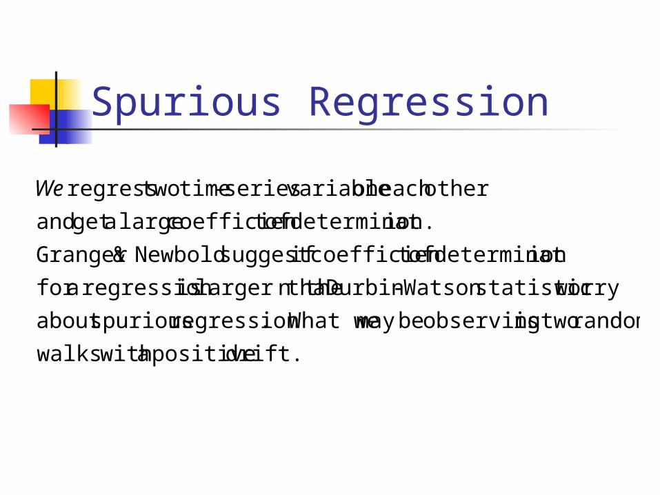
drift. positive a with walks

random twois observing bemay What we.regression spuriousabout

worrystatisticWatson -Durbin n thelarger tha is regression afor

iondeterminat oft coefficien ifsuggest Newbold &Granger

ion.determinat oft coefficien large aget and

othereach on variableseries- time tworegress We

Relate Price level to Money Supply

Coefficients Standard Error t StatIntercept 78.34396361 0.809216059 96.81464M1 0.041353791 0.000947232 43.65753

Note: For this regression R-square=0.888162964

And DW = 0.028682

We have to fear a Spurious regression.

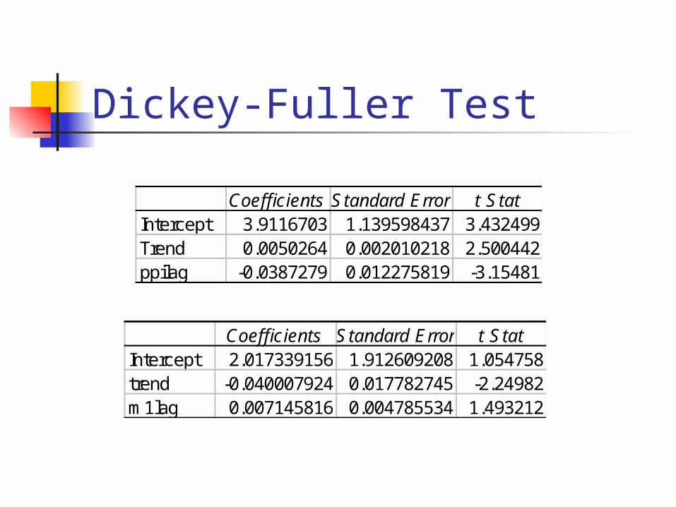
Dickey-Fuller Test

Coefficients Standard Error t StatIntercept 3.9116703 1.139598437 3.432499Trend 0.0050264 0.002010218 2.500442ppilag -0.0387279 0.012275819 -3.15481

Coefficients Standard Error t StatIntercept 2.017339156 1.912609208 1.054758trend -0.040007924 0.017782745 -2.24982m1lag 0.007145816 0.004785534 1.493212

Cointegration We can have two variables trending

upward in a stochastic fashion, they seem to be trending together. The movement resembles two dancing partners, each following a random walk, whose random walks seem to be unison.

Synchrony is intuitively the idea behind cointegrated time series.

Cointegration

ed.cointegrat are X and Y variablesthe

say then wenoise, whiteI(0), is if

ly,specifical More .stationary bemay variables twothe

ofn combinatiolinear a thisDespite . variables)I(1

are both which X, and Y , variables twohavemay We

21t tt XY

Cointegration We need to check the residuals from

our regression to see if they are I(0). If the residuals are I(0) or stationary,

the traditional regression methodology (including t and f tests) that we have learned so far is applicable to data involving time series.

Test for Cointegration

root.unit have errors that hypothesis nullreject

notcan We0.029. DW was theexample,money on ppiour For

tests.10% and 5% 1%,for 0.322 and 0.386 0.511, are

valuesCutoff test.-DW standardfor 2d versus0dbut test

,regressionour for statisticDW get the weCRDW test In the

Watson-Durbin Regression ingCointegrat 2.

residuals. thet toFuller tes-Dickey apply thecan We.1

Cointegrating regression: PPI and M1

OINTEGRATING REGRESSION - CONSTANT, NO TREND NO.OBS = 242 REGRESSAND : PPIACO R-SQUARE = 0.8882 DURBIN-WATSON = 0.2868E-01 DICKEY-FULLER TESTS ON RESIDUALS - NO.LAGS = 14 M = 2 TEST ASY. CRITICAL STATISTIC VALUE 10% --------------------------------------------------------------------------- NO CONSTANT, NO TREND T-TEST -2.4007 -3.04 AIC = -1.200 SC = -0.974 ---------------------------------------------------------------------------

Error Correction Model

tttt

ttt

XYX

X

)(

ˆY

m.equilibriurun

long toadjustmentrun short get to tomodel correctionerror use We

. variablesebetween th iprelationshrun long aexist

e then ther,regression ingcointegrat a have weIf

1211210

1210t

Error Correction model: exchange rate & interest Rate

Coefficients Standard Error t StatIntercept 84.4016519 1.934688878 43.62544BA6M 1.82542313 0.24291891 7.514537

Regression of exchange rate on interest rate

Error Correction Model

Coefficients Standard Error t StatIntercept -0.0369947 0.095387016 -0.38784diffintr 0.7803093 0.153370941 5.087726Residuals -0.0153463 0.007787867 -1.97054