1

Economic Reforms and Gender-based Wage Inequality in the Presence of Factor Market

Distortions♣♣♣♣

Sarbajit Chaudhuri, Dept. of Economics, University of Calcutta, India

and

Somasree Roychowdhury, Dept. of Economics, Lady Brabourne College, Kolkata, India

Address for communication: Sarbajit Chaudhuri, 384/1, M.B. Road, Nimta, Belgharia, Kolkata

700049, India. Tel: 91-9830530963 (M), 91-33-2557-5082 (C.U.). Fax: 91-33-2844-1490 (P). E-

mail: sarbajitch@yahoo.com

(This version: May 14, 2014)

Abstract: A simple three-sector general equilibrium model has been developed with both male

and female labour and factor market distortions. The effects of different liberalized economic

policies have been examined on the gender-based wage inequality. The analysis finds that credit

market reform and tariff reform produce favourable effects on the wage inequality while the

liberalized investment policy becomes counterproductive. These results have important policy

implications for a small open developing economy.

Keywords: Male labour, female labour, gender wage inequality, labour market distortion, credit

market distortion, economic reforms, general equilibrium.

JEL classifications: D50, J16, F21.

♣♣♣♣ The authors are thankful to Prof. Ishita Mukhopadhyay for her helpful comments on an earlier version

of the paper. The usual disclaimer, however, applies.

2

Economic Reforms and Gender-based Wage Inequality in the Presence of Factor Market

Distortions

1. Introduction

Gender empowerment impacts the quality and efficiency of decision making and resource

allocation, which is relevant for social and economic development. Gender inequality, in terms

of access to education, health facilities and credit is a predominant feature of most developing

countries. Women also face gender discrimination in the labour market and financial market,

limiting the economic progress of countries. The discrimination in the labour market between

men and women can be observed in all countries, although it is much more pronounced in the

developing countries.

While the manifestations of gender discrimination are multi-dimensional and intertwined, an

overreaching phenomenon is gender wage inequality. Gender wage discrimination not only, by

itself, represents an inequality, but also is a reason of many other types of gender inequalities.

Low wages for women leads to economic dependence and thereby their lower social status and

decision making position in society. The reason(s) for gender wage gap is a very contentious

issue and various schools of thought have endeavored to ascribe reasons for the same. The neo-

classical view is that free markets, through the competition process, ensure that wage

differentials are eliminated. The cultural historians are of the view that gender wage differentials

are because of cultural/societal stereotyping of women’s work for low-end, less remunerated

jobs. Such culture-driven occupational segregation persists even under competitive conditions.

Burnette (2008) has, however, through her studies on gender work and wages in the Industrial

Revolution of Britain, concluded that occupational segregation was not the cause of wage gap

but a way to shelter women from “the full force of their lower productivity” caused by their less

physical strength and child care responsibilities. Another school of thought, championed by

Humphries (2009), propounded that powerful elements in society manipulate the various factors

of production to further their wealth and status, which manifests in inequalities, including gender

wage inequality.

3

The size of the gender wage gap varies across countries as well as within the country. In many

countries of Asia, Middle East and North Africa, the gap is upwards of 40% in some sectors

(Corley, Perardel and Popova 2005). In Latin America and the Caribbean, most women earn on

an average 69% of men’s income. In the context of India, gender wage gap at the national level,

on an average, for female labour is 70% of that of daily male wage rate in the agricultural sector

in India (National Sample Survey, 2004). Klaveren et al. (2010) found for 2004-05 a very large

gender pay gap of 57% in the formal (organised) sector. Comparisons with the unorganised

sector showed that wages rates here were 20-30% of those in the organised sector, though wage

rates varied widely across states and activities. Among casual workers, gender pay gaps showed

up of 35-37%. Kornick (2005) has demonstrated in his study that women labour is

predominantly employed in the unorganized sector. The 68th Round of National Sample Survey

(2011-12) has found that women are mainly engaged in rural areas as cultivators and agricultural

labourers and in urban areas, fourth-fifth of the working women are involved in unorganized

sectors such as household industries, petty trade and services, building and construction. Women

make up just a fifth of the organized sector workforce. Since the proportion of women working

in unorganized sector is high, the overall average daily wage rate of women labour gets

depressed.

The developing countries have chosen free trade as their development strategy and been

vigorously implementing various liberalized economic policies over the last three decades. The

ongoing process of globalization must have produced a significant impact on the gender-based

wage inequality. These policies change the relative factor prices and lead to reallocation of

factors of production among sectors that use them with different intensities and thereby change

their employment and wages. Therefore liberalization policies affect the choice of employment

between men and women workers and their respective remunerations (UNCTAD 1999).

Several empirical studies have tried to find out the impact of trade openness to gender wage

inequality although their findings of the consequences on the inequality have been mixed in

nature. For example, Berik (2000), Fontana and Wood (2000), Oosetendorp (2009), Dell (2005),

Artecona and Cunningham (2002), Garcia-Cuellar (2001) have shown that increased volume of

4

trade due to openness has caused the expansion of female levels of participation and decreased

the gender wage inequality. On the contrary, there are several other studies like Artecona and

Cunningham (2002), Dutta Gupta (2002), Fontana (2002), Berik, Rodgers,and Zveglich (2004)

which show that trade openness has increased the gender wage inequality.

Studies like Menon and Rodger (2009), Chamarbagwala (2006), Bhattacharya and Rahaman

(1999) have concentrated on the impact of different liberalization policies, such as tariff

reduction, deregulation of licensing, etc in developing countries like India, Pakistan Bangladesh

and South Asian economies. These studies concluded that trade liberalization widened the

gender pay gap. It was found that women are generally more constrained than men from reaping

the benefits from the expansion of trade in agriculture.

Most of the work done on gender wage gap and economic liberalization are empirical in nature.

However, there should be a theoretical literature that can be useful in analyzing the consequences

of different liberalized economic and other policies on the gender wage inequality in a simple

general equilibrium structure and be useful in prescribing policy measures based on the

theoretical findings that can be useful for mitigating the gravity of the problem. The theoretical

literature in this area has not emerged as yet. However, mention should be made of a paper by

Mukhopadhyay and Chaudhuri (2013) (MC (2013) hereafter) which has examined the

consequences of trade reform and inflow of foreign capital on gender wage inequality and

welfare of the economy in a developing economy in terms of a three-sector general equilibrium

model. In this paper we have also made an attempt in analyzing the outcomes of different

liberalized economic policies e.g. trade reform, credit market reform and investment reform on

the gender-based wage inequality by using a three-sector full-employment general equilibrium

model with both male and female labour.

The present work is, however, different from that of MC (2013) in a number of ways. First, in

MC (2013) any convincing explanation as to why the gender wage gap arises has not been

provided. Here we have tried to offer quite a few of such explanations in terms of differences in

5

calorie intakes, spending patterns and physiological factors1 between men and women. Second,

while MC (2013) considered a competitive male labour market we have considered a formal-

informal segmentation of the male labour market which is closer to reality especially in the

context of a developing economy.2 Third, we allow capital mobility between the female labour

oriented export sector (sector 2) and the formal import-competing sector (sector 3) whereas in

MC (2013) capital mobility is allowed only between the two informal sectors. Actually, sector 1

is agriculture that uses a special type of capital: land, while capital is used in the other two

sectors is basically ‘working capital’. So, specificity of land to agriculture and free mobility of

working capital between the other two sectors, as in our case, is more realistic relative to MC

(2013). Fourth, the present work considers the role of the capital market imperfection, which is a

salient feature of the developing countries like India in explaining the gender wage differential

which is not dealt in MC (2013). Finally, our results are more distinct and involve less

parametric restrictions that lead to stronger policy implications relative to their work.

2. The Model

We develop a simple three-sector, full-employment general equilibrium model for a small open

developing economy with four inputs.3 The four inputs of production are male labour ( M ),

female labour ( F ), land ( N ) and capital ( K ). Here capital means working capital.

1 According to Gustafsson and Lindenfors (2004) most males are stronger than females. See also

http://en.wikipedia.org/wiki/Sex_differences_in_humans in this context.

2 The female labour market in a developing country is also segmented. However, we have excluded

female labour in the formal manufacturing sector (sector 3) of the economy owing to the empirical fact

that only a very small proportion of the aggregate female labour force is employed in that sector and that

on an average the female share in trade union membership and decision-making is low (Klaveren et al.

2010). See also footnote 5 in this context.

3 Unemployment of either type of labour is a disconcerting problem in a developing economy. However,

we do not consider unemployment in our model because our only objective here is to examine the

possible consequences of economic reforms on the gender-based wage inequality. This point has been

elaborated further in the concluding section.

6

Sector 1 is an informal sector that produces an exportable agricultural commodity, 1X (say food),

using male labour, female labour and land. Sector 2 is a female labour-oriented informal sector

that produces also an export good, 2X by means of female labour and capital. A classic example

of such a sector, in the developing countries, would be the booming garment industry in

Bangladesh, which is both female worker and export oriented (Kornick 2005). A few other such

industries in the developing economies are: tea, tobacco and food-processing.4 Sector 3 is

organized formal sector that produces a manufacturing good, 3X , (e.g. machinery and equipment,

transport equipment, basic metals, fabricated metal products etc.) with the help of male labour

and capital. This is the tariff-protected import-competing sector of the economy. We exclude

female labour in the production of commodity 3 primarily because the percentage of female

labour used in the production activities mentioned above is insignificant (see Chaudhuri and

Panigrahi (2013), Table 2).5, 6

Male workers in the agricultural sector (sector 1) earn the competitive wage, M

W , while the male

wage rate in the manufacturing sector (sector 3) is *

MW , which is institutionally determined, and

*

M MW W> . The male labour allocation mechanism is as follows. Male workers first compete for

getting jobs in sector 3 where the wage rate is high due to institutional reasons. But those who

cannot get employment in that sector are automatically absorbed in sector 1 providing the

4 See Mukhopadhyay and Chaudhuri (2013), footnote 9 in this context.

5 See also Selected Socio-Economic Statistics (SSES), India 2011 in this context.

6 It is extremely important to mention that even if female labour were included in the manufacturing

sector and their participation in trade union activities were the same as their male counterparts, the

average female wage would have been much lower than the average male wage. This is due to the fact

that the proportion of aggregate female workforce employed in the formal sector is very low vis-à-vis the

male workforce and that there exists a substantial gender wage gap in the informal sector including

agriculture. Besides, empirical studies e.g. SSES, India (2011) and Klaveren et al. (2010) show that the

percentage of female workforce employed in the formal sector is significantly low and that on average the

female share in labour union membership and decision-making is low. Hence, there is no harm if the use

of female labour is assumed away in sector 3 for analytical simplicity. Furthermore, it may intuitively be

checked that the qualitative results of the model get through even if one includes female labour in sector

3.

7

competitive and low wage. So we have distortions in the male labour market. The female labour

market is, however, perfect.7 Land is specific to sector 1.

Capital flows freely between sector 2 and sector 3 although the former sector faces a higher cost

of capital vis-à-vis the latter due to capital market imperfections. Owing to the assumption of a

small open economy, commodity prices are internationally given. The endowments of the four

primary inputs in the economy are , ,M F K and N which are given exogenously. All the factors of

production are fully employed. Production functions in all the sectors exhibit constant returns to

scale with diminishing marginal productivity to each factor.

2.1 A few explanations for the existence of gender wage gap

We now provide a few explanations why the gender wage gap exists even in the competitive

labour markets. The ICMR (2010, Table 4.1) report has pointed out that the minimum calorie

requirement of a male worker to maintain the same level of productivity or efficiency is higher

than that of a female worker. Furthermore, the spending patterns of the male and female workers

are significantly different. Women are more likely than men to spend a significantly higher

proportion of their income on purchases of goods and services that promote the nutrition, health

and general well being of their families (Duncan 1997; Quisumbing et al. 1998; Kurz and Welch

2000). Men tend to spend most of their income on non-food items and their personal luxury

articles like alcohol and cigarettes or reinvest it in their work or businesses (Guyer 1988;

Hoddinott and Haddad 1995; Anderson and Baland 2002).

The physical efficiency of male labour is greater than that of female labour.8 This difference may

arise due to biological difference or the difference in calorie intakes and the resulting nutritional

7 See footnotes 2 and 6 in this context.

8 This is analogous to the productivity difference between adult labour and child labour. In the literature

on child labour the productivity of adult labour has been considered to be significantly greater than that of

child labour simply because of the biological reason although in different informal sectors these two types

of labour are substitutes. The difference in labour productivities results in their wage differential. See for

8

difference between the two types of labour. Indian women are traditionally more concerned

about the well-being and nutritional status of their husbands and children relative to those of

their own. This may be one of the main reasons why malnutrition is much pronounced among

women, especially in the rural areas of the developing economies including India.

If we keep all these in mind it is not unreasonable to assume that in a largely male-dominated

working household the male and female workers consume exactly those amounts of food

(commodity 1 in the present model) just sufficient enough to maintain their existing physical

productivities.9 The family income in excess of that amount is spent on non-food items and

luxury goods of the male worker and on children’s welfare that do not contribute to their

productivities directly.

In mathematical terms, the efficiency of a male worker, denotedm

h , is given by

(c )m m

h h= with (.) 0, (.) 0h h′ ′′> < (1)

where m

c = (minimum) amount of calorie intake by a male labour.

Similarly, the efficiency of a female labour, F

h , is

( )f fh h c= with (.) 0, (.) 0h h′ ′′> < (2)

wherefc = (minimum) amount of calorie intake by a female labour.

Clearly, m fh h> as

mc >

fc . As commodity prices are internationally given by the small open

economy assumption, the amounts of expenditures required for m

c and fc calorie intakes are

example, Basu and Van (1998), Chaudhuri and Dwibedi (2006, 2007, 2010) etc. It may, however, be

mentioned that an extra-economic factor that a child worker usually has a very little power over his labour

supply decision is also a reason behind the existence of this wage differential.

9 This may not be the case of male workers employed in sector 3 where they receive a high unionized

wage which is greater than the competitive male wage in sector 1. If male workers in sector 3 consume

more calories than,m

c , level the productivity of each of them is likely to be higher than their counterparts

in sector 1. However, for simplifying matters and keeping our analysis focused on the gender wage

inequality the possibility of such a productivity differential is assumed away.

9

also given. This can possibly be an economic explanation for the wage disparities between male

wage and female wage. These arguments seem to be more convincing if the physiological

difference between the two types of labour as highlighted by Gustafsson and Lindenfors (2004)

is also taken into consideration. So, we can write

MW >

FW where

MW and

FW stand for the

competitive male and female wages, respectively. It is important to mention here that although

the gender wage gap exists the absolute wages of the two types of labour in the informal sectors

and the magnitude of the wage gap in our model are determined by competitive forces.10

2.2 The General Equilibrium framework

The general equilibrium structure of the model is represented by the following set of equations.

1 1 1 1M M F F N

W a W a Ra+ + = (3)

2 1 2 2F F KW a r a P+ = (4)

* *

3 2 3 3 3(1 )M M KW a r a P t P+ = + = (5)

Equations (3) – (5) are the three competitive industry equilibrium i.e. zero-profit conditions.

Here, jia is the amount of the j th factor required to produce 1 unit of output of the i th sector

with , , ,j M F L K= and 1, 2,3i = ; i

P = the internationally given price of the i th commodity with

2,3i = . t is the ad-valorem rate of tariff on sector 3. The other symbols have already been

defined. Finally, commodity 1 is taken to be the numeraire.

10 Due to existence of imperfections in the market for male labour in the organized sector (sector 3) the

male workers receive the unionized wage which is institutionally determined while their counterparts in

the agricultural sector (sector 1) receive a low competitive wage. For a theory of determination of the

unionized wage in the formal sector one may go through Chaudhuri (2003) and Chaudhuri and

Mukhopadhyay (2009) among others.

10

At this point, it should be pointed out that male labour and female labour are used in different

sectors of the economy as separate inputs. They are substitutes to each other but not perfect

substitutes. If they were perfect substitutes the competitive female wage, F

W , would have been

equal to (f

M

m

hW

h) and instead of separate male and female labour markets there would have been

only one labour market.11

This is analogous to the degree of substitutability between adult

labour and child labour in the literature on child labour. In Basu (1999), in order to explain the

possibility of multiple equilibria in the in the simplest possible manner it has been assumed that

adult labour and child labour are perfect substitutes. In other words, children can do whatever

adults do. However, this is an oversimplification of reality. In Chaudhuri and Dwibedi (2006,

2007, 2010) adult labour and child labour have been considered to be substitutes but not perfect

substitutes.

We have assumed capital market imperfection in the economy.12

The cost of capital in sector 2 is

higher than that in sector 3. The relationship between the two interest rates is given as follows.

1 2r rβ= (6)

Here, β is a parameter which is determined by institutional characteristics of the credit market

and 1β > implies capital market imperfections.13

It is easily seen that 1 2r r> if 1β > .

11 Government of India (2010) has reported that in some of the activities within agriculture like tractor

driving, women are not used and in many other cases the gender wage gap cannot strictly be explained by

productivity difference rather than by competitive forces.

12 The informal sector firms being unregistered in nature have very little access to the organized credit

market. They are bound to borrow a lion’s share of their working capital from the informal sector lenders.

On the other hand, these exploitative lenders due to their easy access to the formal capital market add on,

largely, unregulated margins for re-lending to the informal sector borrowers. This raises the cost of

financing of the unorganized sector. These characteristics of the informal credit market have been

adequately described and analyzed in Bhaduri (1977), Rudra (1982), Basu (1998), Basu and Bell (1991),

Mishra (1994), Chaudhuri (2003) and Chaudhuri and Mukhopadhyay (2009). For a theory of

determination of the informal interest rate in a general equilibrium structure, beginning from the

microeconomic behaviour of the informal sector lender in an imperfectly competitive credit market, one

may go through Chaudhuri and Gupta (2014).

11

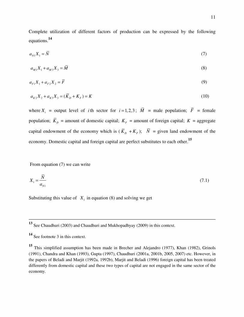
Complete utilization of different factors of production can be expressed by the following

equations.14

1 1Na X N= (7)

1 1 3 3M Ma X a X M+ = (8)

1 1 2 2F Fa X a X F+ = (9)

2 2 3 3 ( )K K D Fa X a X K K K+ = + = (10)

wherei

X = output level of i th sector for 1, 2,3i = ; M = male population; F = female

population; DK = amount of domestic capital;

FK = amount of foreign capital; K = aggregate

capital endowment of the economy which is (DK +

FK ); N = given land endowment of the

economy. Domestic capital and foreign capital are perfect substitutes to each other.15

From equation (7) we can write

1

1N

NX

a= (7.1)

Substituting this value of 1X in equation (8) and solving we get

13 See Chaudhuri (2003) and Chaudhuri and Mukhopadhyay (2009) in this context.

14 See footnote 3 in this context.

15 This simplified assumption has been made in Brecher and Alejandro (1977), Khan (1982), Grinols

(1991), Chandra and Khan (1993), Gupta (1997), Chaudhuri (2001a, 2001b, 2005, 2007) etc. However, in

the papers of Beladi and Marjit (1992a, 1992b), Marjit and Beladi (1996) foreign capital has been treated

differently from domestic capital and these two types of capital are not engaged in the same sector of the

economy.

12

13

3 1

1( )( )M

M N

aX M N

a a= − (8.1)

Similarly substituting the value of 1

X in equation (9) and solving we get

12

2 1

1( )( )F

F N

aX F N

a a= − (9.1)

Then, using equations (8.1), (9.1) and (10) we can find

32 1 1

2 1 3 1

( )( ) ( )( )KK F M

F N M N

aa a aF N M N K

a a a a− + − = (10.1)

There are eight endogenous variables in the system: M

W , F

W , R , 1r ,

2r ,

1X ,

2X ,and

3X and

exactly the same number of independent equations, (3) – (10). This is an indecomposable

production structure. Some of the factor prices depend on both commodity prices and factor

endowments. Therefore, any changes in the factor endowments will affect some of the factor

prices, which in turn affect the factor-coefficients. The policy parameters of the system are β , t

and K .

The endogenous variables are determined as follows. 2

r is determined from equation (5) as *

MW is

exogenously given. Once 2

r is obtained 1r is solved from equation (6). Then

FW is determined

from equation (4). So, these three depend only on commodity prices. M

W and R are obtained by

solving equation (3) and equation (10.1) simultaneously. Once factor prices are determined,

factor coefficients are also obtained as these are functions of factor prices. From equation (7) we

can determine the value of1

X . Finally, from equations (8.1) and (9.1), 3

X and 2

X are

determined, respectively.

13

The male workers in this model work either in sector 1 or in sector 3 earning M

W and *

MW wages,

respectively. The average male wage is denoted by a

MW where

a

MW = *

1 3M M M MW Wλ λ+ (11)

Here 1M

λ and3M

λ denote the proportions of male labour employed in sector 1 and sector 3,

respectively and 1 3

( ) 1M M

λ λ+ = .

So, *

3 ( )a

M M M M MW W W Wλ= + − (11.1)

The absolute gender wage gap is ( )a

M FW W− implying that the average male wage rate is greater

than the female wage rate. The relative gender wage inequality, denoted I , is given by

ˆ ˆ( )a

M FI W W= −

(12)

Here ‘ ∧ ’ implies proportional change e.g. ˆ ( )FF

F

dWW

W= .

The relative gender wage inequality worsens (improves) due to any policy changes if

( )ˆ ˆ ( ) 0a

M FW W− > <

i.e. if ( ) 0I > < .

3. Comparative statics

In this section of the paper we attempt to examine the effects of different liberalized economic

policies like credit market reform, trade reform, and an inflow of foreign capital on the gender

wage inequality in the existing set-up. A credit market reform is captured through a reduction

in β . A trade reform can be encapsulated through a reduction in the ad-valorem tariff rate, t .

Finally, a policy of investment liberalization in this model means an increase in the endowment

of the foreign capital in the economy i.e.F

K .

14

Differentiating equation (5) we obtain

2

3

ˆˆ

K

Ttr

θ=

(13)

where,

( /1 ) 0T t t= + >

Then totally differentiating equation (6) and using (13) one finds

1

3

ˆˆˆ

K

Ttr β

θ= +

(14)

Differentiating equation (4), using (14) and simplifying we obtain

2

2 3

ˆˆˆ ( )( )K

F

F K

TtW

θβ

θ θ= − −

(15)

Totally differentiating equation (11.1) we find

312 3*

ˆ ˆ ˆˆ[( ) (1 )(S )]a M M MM M MKa

M M

W WW W r X

W W

λ= + − +

(16)

Using equations (15), (16) from (12) we finally find that

312 3*

ˆ ˆ ˆˆ( ) (1 )(S )}[{ ]M M MM MK Fa

M M

W WI W r X W

W W

λ= + − + −

(17)

Here jiθ and jiλ

respectively denote the distributive and allocative shares of the jth input in

theith sector for

, , ,j M F N K= and

1, 2,3i =.

i

jkS = the degree of substitution between factors

j and k in the i th sector, , , , ,j k N M F K= ; and, i = 1,2,3.€16

Using equations (15) – (17) the following propositions can easily be established.17, 18

16 See the Appendix for detailed definition.

15

Proposition 1: A policy of credit market reform is quite likely to improve the gender wage

inequality.

Proposition 2: Trade reform in the form of a reduction in the rate of import tariff lowers the

gender-based wage inequality under reasonable conditions.

Let us now explain these results in economic terms. A policy of credit market reform, captured

through a reduction in the degree of credit market imperfection ( β ) lowers the power of the

exploitative informal sector lenders and hence their ability to mark up interest rate over the

competitive rate (2

r ). So, the informal interest rate (1r ) falls (equation 6) although

2r does not

change. Then from the zero-profit condition for sector 2 (equation 4) it follows that the female

wage (F

W ), rises. Sector 2 expands as the effective price of its product net of capital cost has

increased.19

However, producers in this sector would substitute female labour by capital as the

latter input has become relatively cheaper. The expanding sector 2 requires more capital which

must come from sector 3 (note that all factors are fully utilized). Sector 3 contracts both in terms

of output and employment of male labour for want of capital. Male workers who have lost their

jobs in the formal sector that pays a higher unionized wage ( *

MW ) now move to sector 1

depressing the competitive male wage (M

W ). As sector 1 now absorbs more male labour than

before, the proportion of male employment to total male endowment i.e. 1M

λ rises

and3M

λ decreases. Quite naturally the average male wage ( a

MW ) falls (equation 16). As the

female wage (F

W ) has already risen the male-female wage inequality improves (equation 17).

17 See the Appendix in this context.

18 These require a sufficient condition. See the Appendix.

19 This happens under a sufficient condition involving parameters of the system. See the Appendix for

details.

16

On the other hand, a policy of trade reform lowers the ad-valorem rate of tariff ( t ) on the import

of commodity 3 that lowers the domestic price of that commodity i.e.3(1 )P t+ . The competitive

return to capital (2

r ) falls as the unionized male wage ( *

MW ) is given (equation 5). This lowers

the interest rate in sector 2 (see equation 6). This leads to an increase in the female wage rate

(F

W ) (equation 4). As3(1 )P t+ has decreased sector 3 contracts both in terms of output and

employment of male labour; thereby, releasing capital to sector 2 and male labour to sector 1.20

This depresses the competitive male wage in sector 1 (M

W ). More male labour are now

employed in the lower wage-paying sector (note that *

M MW W> ) . This means that1M

λ rises and

hence3M

λ falls. Quite naturally, the average male wage ( a

MW ) plummets (equation 16). The

gender wage inequality improves as the female wage (F

W ) has already increased (equation 17).

Finally, we would like to analyze the consequence of the liberalized investment policy on the

gender-based wage inequality. The liberalized investment policy in the present context implies

an inflow of foreign capital inflow. If there occurs an inflow of foreign capital, the foreign

capital stock of the economy (F

K ) goes up. Both sector 2 and sector 3 expand as they use

capital. Sector 3 now demands more male labour which comes from sector 1 while the demand

for female labour rises in sector 2 which is met by release of female labour by sector 1.

Consequently, the competitive male wage (M

W ) increases because its demand in the economy

has increased and M

W depends on both factor endowments and commodity prices. Although the

demand for female labour has also increased the female wage (F

W ) cannot rise as it is

determined from the zero-profit condition of sector 2 (equation 4). Note that 2 1,r r and

FW are

determined from equations (5), (6) and (4), respectively. So, we find that the competitive male

20 This happens subject to a sufficient condition which is stated in the Appendix. It is to be noted that the

cost on capital has also fallen in sector 3 that leads the producers to substitute male labour by capital

which results in an increase in 3K

a . So, the expansion of sector 2 depends on whether the contracting

sector 3 actually demands less capital than before. However, sector 3 releases capital and sector 2 in fact

expands subject to a sufficient condition as mentioned above.

17

wage (M

W ) and the proportion of male labour employed in the higher wage-paying sector have

increased leading to an increase in the average male wage in the economy ( a

MW ). The gender-

based inequality unambiguously deteriorates (rises). This leads to the final proposition of the

model.

Proposition 3: The liberalized investment policy in the form of inflows of foreign capital

unambiguously worsens the male-female wage inequality.

4. Concluding remarks and policy implications

The gender-based wage inequality in the labour market is a persistent problem across countries,

especially the developing ones. The developing economies have been vigorously implementing

the liberalized economic policies over the last three decades which must have important

consequences on the problem. We have developed a simple three-sector general equilibrium

model with both male and female labour and factor and commodity market distortions with a

view to examine the impacts of liberalization drives by the developing nations on the gender

wage inequality. We have found that policies of credit market reform and tariff reform produce

favourable effects on the inequality while the liberalized investment policy becomes

counterproductive. The policy recommendations that readily follow from the results are to go for

credit market and trade reforms vigorously. But, the policymakers should be careful in

implementing the investment reform as it is likely to backfire unless the policy is accompanied

by credit market reformatory policies like curbing the power of the exploitative informal lenders

by allowing small firms in the informal sector to borrow their working capital from the organized

credit market at the competitive rate. This would help these firms to grow and their demand for

female labour to pick up significantly. Consequently, the female wage rises that lowers the

gender wage inequality. If these supplementary policies are undertaken the liberalized

investment policy would not only lead to a balanced growth of the economy but also definitely

improve the gravity of the inequality problem.

18

Finally, it should be mentioned that in the present work we have analyzed the possible outcomes

of different liberalized economic policies on the male-female wage inequality in the simplest

possible manner. Some of the assumptions like exclusion of female labour in the formal sector of

the economy and classification of both types of labour according to their skills and absence of

non-traded goods are restrictive. Furthermore, the determination of the supply of each type of

labour from the maximizing behaviour of a working household could be an interesting exercise.

Our future research should address these aspects.

References:

Anderson, S. and Baland, J. M. (2002): ‘The economics of Roscas and intra-household resource

allocation’, The Quarterly Journal of Economics 117(3), 963-995.

Artecona, R. and Cunningham,W. (2002): ‘Effects of trade liberalization on the gender wage gap

in Mexico’, Gender and Development working paper series 21 The World Bank Development

Group.

Basu, K. (1999): ‘Child Labour: Cause, Consequence, and Cure, with Remarks on International

Labour Standards’, Journal of Economic Literature, 37(3), 1083-1119.

Basu, K. (1998): Analytical Development Economics – The Less Developed Economy Revisited,

Oxford University Press, Delhi.

Basu, K. and Van, P. H. (1998): ‘The economics of child labour’, American Economic Review,

88(3), 412-427.

Basu, K. and Bell, C. (1991): ‘Fragmented duopoly: theory and applications to backward

agriculture’, Journal of Development Economics 36, 259-81.

Beladi, H. and Marjit, S. (1992a): ‘Foreign Capital and Protectionism’, Canadian Journal of

Economics, 25, 233-238.

Beladi, H. and Marjit, S. (1992b): ‘Foreign Capital, Unemployment and National Welfare’,

Japan and the World Economy, 4, 311-317.

Berik, G., Rodgers, Y. and Zveglich, J. (2004): ‘International trade and gender wage

discrimination: evidence from East Asia’, Review of Development Economics, 8(2), 237-254.

Berik, G. (2000): ‘Mature export-led growth and gender wage inequality in Taiwan’. Feminist

Economics 6(3), 1–26.

19

Bhaduri, A. (1977): ‘On the formation of usurious interest rates in backward agriculture’,

Cambridge Journal of Economics1 4, 341-352.

Bhattacharya, D. and Rahaman, M. (1999): ‘Female employment under export propelled

industrialization: Prospects for internalizing global opportunities in the apparel sector in

Bangladesh’, Occasional Paper no. 10, (UNRISD), Geneva.

Brecher, R. A. and Diaz Alejandro, C. F. (1977): ‘Tariffs, Foreign Capital and Immiserizing

Growth’, Journal of International Economics 7, 317–322.

Burnette .J. (2008): Gender, Work and Wages in Industrial Revolution Britain’. Cambridge

University Press, Cambridge.

Chamarbagwala, R. (2006): ‘Economic liberalization and wage inequality in India’, World

Development 34(12), 1997–2015.

Chandra, V. and Khan, M. A. (1993): ‘Foreign Investment in the Presence of an Informal

Sector’, Economica, 60, 79-103.

Chaudhuri, S. (2003): ‘How and how far to liberalize a developing country with informal sector

and factor market distortions’, Journal of International Trade and Economic Development 12(4),

403-428.

Chaudhuri, S. and Mukhopadhyay, U. (2009): Revisiting the Informal Sector: A General

Equilibrium Approach. Springer, New York.

Chaudhuri, S. and Gupta, M. R. (2014): ‘International factor mobility, informal interest rate and

capital market imperfection: a general equilibrium analysis’, Economic Modelling 37(C), 184-

182.

Chaudhuri, S. and Dwibedi, J. K. (2007): ‘Foreign capital inflow, fiscal policies and the

incidence of child labour in a developing economy’, The Manchester School 75(1), 17- 46.

Chaudhuri,S and Dwibedi, J. K. (2006): ‘Trade liberalization in agriculture in developed nations

and incidence of child labour in a developing economy’, Bulletin of Economic Research 58(2),

129-150.

Chaudhuri, S. (2001a): ‘Foreign capital Inflow, technology transfer, and national income’, The

Pakistan Development Review, 40 (1), 49-56.

Chaudhuri, S. (2001b): ‘Foreign capital inflow, non-traded intermediary, urban unemployment,

and welfare in a small open economy: A theoretical analysis’, The Pakistan Development

Review, 40 (3), 225-235.

20

Chaudhuri, S. (2005): ‘Labour market distortion, technology transfer and gainful effects of

foreign capital’, The Manchester School, 73(2), 214-227.

Chaudhuri, S. (2007): ‘Foreign capital, welfare and unemployment in the presence of agricultural

dualism’, Japan and the World Economy, 19(2), 149-165.

Chaudhuri, B. and Panigrahi.A. K. (2013): ‘Gender bias in Indian industry’; The Journal of

Industrial Statistics 2(1) 108-127.

Corley, M., Perardel, Y. and Popova, K. (2005): ‘Wage inequality by gender and occupation: a

cross-country analysis’, Employment Strategy Papers No. 20, International Labour Office.

Datta Gupta, N. (2002): ‘Gender, pay and development: a cross-country analysis,’ MPRA

Paper 15311, University Library of Munich, Germany.

Dell, M. (2005): ‘Widening the border: The impact of NAFTA on female labor force

participation in Mexico’, Oxford University, UK.

Duncan, T. (1997): ‘Incomes, expenditures and health outcomes: Evidence on intrahousehold

resource allocation’, in Haddad, L., Hoddinott, J. and Alderman, H. (eds.), Intrahousehold

Resource Allocation in Developing Countries: Models, Methods and Policy, Baltimore and

London. The Johns Hopkins University Press.

Dwibedi, J. K. and Chaudhuri, S. (2010): ‘Foreign capital, return to education and child labour’,

International Review of Economics and Finance 19(2), 278-286.

Fontana, M. (2002): ‘Modelling the effect of trade on women at work and at home: A

comparative perspective’. Paper presented at SIAP Workshop, 7–8 November, in Brussels,

Belgium. http://www.cepii.fr/anglaisgraph/communications/pdf/2002/siap1102/fontana.pdf

Fontana, M., and A. Wood (2000): ‘Modelling the effects of trade on women, at work and at

home’, World Development 28(7), 1173–90.

Garcia-Cuellar, R (2001): ‘Essays on the effects of trade and location on the gender gap: A study

of the Mexican labor market’, Harvard University, Economics Department, Doctoral Dissertation

working Paper.

Grinols, E. L. (1991): ‘Unemployment and foreign capital: The relative opportunity cost of

domestic labour and welfare’, Economica, 57, 107-121.

Gupta, M. R. (1997): ‘Foreign capital and informal sector: Comments on Chandra and Khan’,

Economica, 64, 353-363.

21

Gustafsson A and Lindenfors P (2004): ‘Human size evolution: No allometric relationship

between male and female stature’; Journal of Human Evolution 47 (4), 253–

266. doi:10.1016/j.jhevol.2004.07.004. PMID 15454336.

Guyer, J. (1988): ‘Dynamic approaches to domestic budgeting: Cases and methods from Africa’,

in Dwyer, D. and Bruce, J. (eds.), A Home Divided: Women and Income in the Third World,

Stanford.

Hoddinott, J., and Haddad, L. (1995): ‘Does female income share influence household

expenditure? Evidence from Cote d’Ivoire’, Oxford Bulletin of Economics and Statistics LVII,

77–97.

Humphries, J. (2009): ‘The gender gap in wages: Productivity or prejudice or market power in

pursuit of profits’, Social Science History 33(4), 481-488.

Government of India (2010): ‘Wage rates in Rural India (2008–2009). Ministry of Labour and

Employment, labour Bureau, Shimla/Chandigarh.

Government of India (2000): Report of the Second National Commission on Labour, NSSO.

ICMR (2010): ‘Nutrient Requirements and Recommended Dietary Allowances for Indians: A

Report of the Expert Group of the Indian Council of Medical Research’, Indian Council of

Medical Research, Hyderabad, India.

Khan, M. A. (1982): ‘Tariffs, foreign capital and immiserizing growth with urban unemployment

and specific factors of production’, Journal of Development Economics, 10, 245–256.

Klaveren, M. V., Tijdens, K., Williams, M. H., Martin, N. R. (2010): ‘India - An Overview of

Women's Work, Minimum Wages and Employment’. Decisions for Life MDG3 Project Country

Report No. 13.

http://www.wageindicator.org/main/Wageindicatorfoundation/wageindicatorcountries/country-

report-india

Korinek (2005): ‘Trade and Gender: Issues and Interactions’ in the OEDC Working Paper.

Kurz, K. M. and Welch, C. J. (2000): ‘Enhancing nutrition results: The case for a women’s

resources approach’, Washington, DC: International Center for Research on Women.

Marjit, S. and Beladi, H. (1996): ‘Protection and gainful effects of foreign capital’, Economics

Letters, 53, 311-326.

Menon, N. and Rodgers, Y. ( 2009): ‘International trade and the gender wage gap: New evidence

from India’s manufacturing sector’, World Development 37(5), 965–81.

22

Mishra, A. (1994): ‘Clientelization and fragmentation in backward agriculture: forward induction

and entry deterrence’, Journal of Development Economics, 45, 271-85.

Mukhopadhyay, U. and Chaudhuri, S. (2013): ‘Economic liberalization, gender wage inequality

and welfare’, Journal of International Trade and Economic Development 22(8), 1214-1239.

National Sample Survey (2011-12): Government of India.

National Sample Survey (2004): ‘Informal Sector and Conditions of Employment in India’,

Government of India.

Oostendorp, R. (2009): ‘Globalization and the gender wage gap’; World Bank Economic Review

23(1), 141–61.

Quisumbing, A. R., Haddad, L., Meinzen-Dick, R. and Brown, L. R. (1998): ‘Gender issues for

food security in developing countries: Implications for project design and implementation’,

Canadian Journal of Development Studies, XIX (Special Issue), 185-208.

Rudra, A (1982): Indian Agricultural Economics: Myths and Realities. Allied Publishers, New

Delhi.

Selected Socio-Economic Statistics (2011): Government of India.

UNCTAD (1999): World Investment Report. New York, United Nations.

Appendix

Totally differentiating equations (3), (4), (5) and (6) one, respectively gets:

1 2ˆ ˆ ˆ ˆˆ ˆ

M FAW ER K Br CW Dr+ = − − − (A.1)

1 1 1ˆ ˆ ˆ

M M N F FW R Wθ θ θ+ = − (A.2)

where: 1 1 1 13 12 1

2 3

[( )( ) ( )( )]K MK FNM FM NM MM

F M

A S S S Sλ λλ λ

λ λ= − + −

2 2 2 2 1 12 12 2

2

[ ( )] 0; [ ( ) ( )( )] 0;K FK KK FK K KF FF NF FF

F

B S S C S S S Sλ λ

λ λλ

= − < = − + − > (A.3)

3 3 1 1 1 13 1 2 13

3 2

( ) 0; [( )( ) ( )( )] 0K M K FK KK MK NN MN NN FN

M F

D S S E S S S Sλ λ λ λ

λλ λ

= − < = − + − <

23

Here, i

jkS = the degree of substitution between factors j and k in the i th sector,

, , , ,j k N M F K= ; and, i = 1,2,3. For example,

1

1 1( / )( / ),MF F M M F

S W a a W≡ ∂ ∂ 1

1 1( / )( / )MM M M M M

S W a a W≡ ∂ ∂ etc. 0i

jkS > for ij ≠ ; and, 0;i

jjS <

It should be noted that as the production functions are homogeneous of degree one, the factor

coefficients, jia s are homogeneous of degree zero in the factor prices. Hence the sum of

elasticities of any factor coefficient (ji

a ) in any sector with respect to factor prices must be equal

to zero. For example, in sector 1, with respect to male labour coefficient, we have

1 1 1( ) 0MM MF MNS S S+ + = while with respect to female labour coefficient, 1 1 1( ) 0FM FN FFS S S+ + = .

Using equations (13) – (15) and simplifying equations (A.1) and (A.2) can be rewritten as

follows.

ˆˆ ˆ ˆ ˆM

AW ER K M Ntβ+ = − − (A.4)

1 1ˆˆ ˆ ˆ

M M NW R Y Ztθ θ β+ = +

(A.5)

where: 2 2

2 3 2

[ ] 0; ( )[ ] 0;K K

F K F

TM B C N B C D

θ θ

θ θ θ= − < = − − <

1 2 1 2

2 2 3

( ) 0; ( ) 0F K F K

F F K

TY Z

θ θ θ θ

θ θ θ= > = > (A.6)

The sign of M is found by using (A.3) while that of N is obtained subject to the following

sufficient condition.

1 1 1 1 1 1( ) ( ) ( )NM MF NF NM NF FM

S S S S S S+ ≤ + ≥ + (A.7)

This condition actually puts some restrictions on the substitution parameters i

jkS s. If the

production functions are of the Cobb-Douglas type, i

jkS s are constants.

24

It may be noted that (A.7) leads to fulfillment of a host of other sufficient conditions

like 1 1

NM FMS S≥ ; 1 1

NF MFS S≥ .

Solving (A.4) and (A.5) one obtains

1 1 1

1 ˆˆ ˆ ˆ( )[ ( ) ( ) ]

( ) (-) (-) (-) (-)( )

M N N NW K M EY N EZ tθ θ β θ= − + − +∆

+ +

1 1 1

1 ˆˆ ˆ ˆ( )[ ( ) ( ) ]

( ) (-) ( )( ) ( )( )( )

M M MR K M AY N AZ tθ θ β θ= − + + + +∆

+ + + − + +

(A.8)

where: 1 1

( ) 0

( ) (-)

N MA Eθ θ∆ = − >

+

It may be noted that

(i) 1

( ) 0M

M AYθ + > ; and, (A.9)

(ii) 1

( ) 0M

N AZθ + >

subject to the fulfillment of the sufficient condition as given by (A.7).

From equations (13) – (15), (A.8) and (A.9) we find that

When ˆ 0K > , (i) 1 2ˆˆ ˆ, , 0Fr r W = ; (ii) ˆ 0MW > ; and, (iii) ˆ 0R < ;

When ˆ 0β < , (i) 1̂ 0r < ; (ii) 2̂ 0r = ; (iii) ˆ 0FW > ; (iv) ˆ 0MW < ; and, (v) ˆ 0R < ; and, (A.10)

When ˆ 0t < , (i) 1̂ 0r < ; (ii) 2̂ 0r < ; (iii) ˆ 0FW > ; (iv) ˆ 0MW < ; and, (v) ˆ 0R < .

25

Totally differentiating equations (7.1), (8.1) and (9.1) we obtain the following three expressions,

respectively.

1 1 1

1 1ˆ ˆ ˆ ˆˆ ( )

(+) (+) (-)

N NM M NF F NNX a S W S W S R= − = − + +

(A.11)

3 1 1 1 1 1 113 2

3

ˆ ˆ ˆ ˆˆ ( )[( ) ( ) ( ) ]

(-) (+)

MMK MM NM M MF NF F MN NN

M

X S r S S W S S W S S Rλ

λ= − − − + − − −

(A.12)

2 2 1 1 1 11 12

3 2 2

ˆˆˆ ˆ ˆ( ) [ ( )( )] ( )( )

(-) (-)

F FFK FF FF NF F FM NM M

K F F

TtX S S S S W S S W

λ λβ

θ λ λ= − + − + − − −

1 11

2

ˆ( )( )

(+)

FFN NN

F

S S Rλ

λ− −

(A.13)

Using (A.10), using (A.7) – (A.9) and simplifying from equations (A.11) – (A.13) we can obtain

the following results.

When ˆ 0K > , (i) 1ˆ 0X < ; (ii) 2

ˆ 0X > ; and, (iii) 3ˆ 0X > ;

When ˆ 0β < , (i) 1ˆ 0X > ; (ii) 2

ˆ 0X > ; and, (iii) 3ˆ 0X < ; and, (A.14)

When ˆ 0t < , (i) 1ˆ 0X < ; (ii) 2

ˆ 0X > ; and, (iii) 3ˆ 0X < .