Embed Size (px)
Citation preview

ECONOMIC GROWTH CENTER YALE UNIVERSITY
P.O. Box 208269 New Haven, CT 06520-8269
http://www.econ.yale.edu/~egcenter
Economic Growth Center Discussion Paper No. 1032
Economics Department Working Paper No. 124
Escaping Famine Through Seasonal Migration
Gharad Bryan London School of Economics
Shyamal Chowdhury
University of Sydney
Ahmed Mushfiq Mubarak* Yale University, School of Management
June 2013
Notes: Center discussion papers are preliminary materials circulated to stimulate discussion and critical comments. *Bryan: London School of Economics, [email protected]. Chowdhury: University of Sydney, [email protected]. Mobarak: Yale School of Management, [email protected]. We are grateful to AusAID, the International Growth Centre and the U.S. Department of Labor for financial support. We thank, without implicating, Tim Besley, Abhijit Banerjee, Judy Chevalier, Esther Duflo, Ted Miguel, Rohini Pande, Ben Polak, Chris Woodruff, John Gibson, Chris Udry, Dean Yang, Michael Clemens, Francisco Rodriguez, Chung Wing Tse, Angelino Viceisza, David Atkin, Peter Schott, Jonathan Feinstein, Mark Rosenzweig, Jean-Marc Robin, four anonymous referees, conference participants at the 20th BREAD conference, 2010 ASSA conference, Federal Reserve Bank of Atlanta, 2011 NEUDC Conference, 2nd IGC Growth Week 2010, 2013 World Bank ABCDE Conference, and seminar participants at Yale University, UCBerkeley,MIT/Harvard, Stanford University, London School of Economics, University of Toulouse, Columbia University, Johns Hopkins University, Inter-American Development Bank, UC-Santa Barbara, World Bank, U.S. Department of Labor, IFPRI, Sacred Heart University and Brown University for comments. Julia Brown, Laura Feeney, Alamgir Kabir, Daniel Tello, Talya Wyzanski, Tetyana Zelenska provided excellent research assistance. This paper can be downloaded without charge from the Social Science Research Network Electronic Paper Collection: http://ssrn.com/abstract=2348362.

Escaping Famine through Seasonal Migration
Gharad Bryan, Shyamal Chowdhury and
Ahmed Mushfiq Mobarak*
June 2013
Abstract Hunger during pre-harvest lean seasons is widespread in the agrarian areas of Asia and Sub-Saharan Africa. We randomly assign an $8.50 incentive to households in rural Bangladesh to out-migrate during the lean season. The incentive induces 22% of households to send a seasonal migrant, their consumption at the origin increases significantly, and treated households are 8-10 percentage points more likely to re-migrate 1 and 3 years after the incentive is removed. These facts can be explained qualitatively by a model in which migration is risky, mitigating risk requires individual-specific learning, and some migrants are sufficiently close to subsistence such that failed migration is very costly. We document evidence consistent with this model using heterogeneity analysis and additional experimental variation, but calibrations with forward-looking households that can save up to migrate suggest that it is difficult for the model to quantitatively match the data. We conclude with extensions to the model that could provide a better quantitative accounting of the behavior.
Keywords: Seasonal Migration, Bangladesh, Risk JEL Codes: O1, O15, J61, R23
*Bryan: London School of Economics, [email protected]. Chowdhury: University of Sydney, [email protected]. Mobarak: Yale School of Management, [email protected]. We are grateful to AusAID, the International Growth Centre and the U.S. Department of Labor for financial support. We thank, without implicating, Tim Besley, Abhijit Banerjee, Judy Chevalier, Esther Duflo, Ted Miguel, Rohini Pande, Ben Polak, Chris Woodruff, John Gibson, Chris Udry, Dean Yang, Michael Clemens, Francisco Rodriguez, Chung Wing Tse, Angelino Viceisza, David Atkin, Peter Schott, Jonathan Feinstein, Mark Rosenzweig, Jean-Marc Robin, four anonymous referees, conference participants at the 20th BREAD conference, 2010 ASSA conference, Federal Reserve Bank of Atlanta, 2011 NEUDC Conference, 2nd IGC Growth Week 2010, 2013 World Bank ABCDE Conference, and seminar participants at Yale University, UC-Berkeley, MIT/Harvard, Stanford University, London School of Economics, University of Toulouse, Columbia University, Johns Hopkins University, Inter-American Development Bank, UC-Santa Barbara, World Bank, U.S. Department of Labor, IFPRI, Sacred Heart University and Brown University for comments. Julia Brown, Laura Feeney, Alamgir Kabir, Daniel Tello, Talya Wyzanski, Tetyana Zelenska provided excellent research assistance.
1 Introduction
This paper studies the causes and consequences of internal seasonal migration in
northwestern Bangladesh, a region where over 5 million people live below the
poverty line, and must cope with a regular pre-harvest seasonal famine (The Daily
Star, 2011). This seasonal famine – known locally as monga – is emblematic of the
widespread lean or “hungry” seasons experienced throughout South Asia and
Sub-Saharan Africa, in which households are forced into extreme poverty for part
of the year.1 The proximate causes of the famine season are easily understood –
work opportunities are scarce between planting and harvest in agrarian areas, and
grain prices rise during this period (Khandker & Mahmud, 2012). Understanding
how a famine can occur every year despite the existence of potential mitigation
strategies is, however, more challenging. We explore one obvious mitigation
option – temporary migration to nearby urban areas that offer better employment
opportunities. We randomly assigned a cash or credit incentive (of $8.50, which
covers the round-trip travel cost) conditional on a household member migrating
during the 2008 monga season. We document very large economic returns to
migration. To explore why people who were induced to migrate by our program
were not already migrating despite these high returns, we build a model with risk
aversion, credit constraints and savings.
The random assignment of incentives allows us to generate among the first
experimental estimates of the effects of migration. Estimating the returns to
migration is the subject of a very large literature, but one that has been hampered
1 Seasonal poverty has been documented in Ethiopia (Dercon & Krishnan, 2000), where poverty and malnourishment increase 27% during the lean season, Mozambique and Malawi (Brune et al., 2011) – where people refer to a “hungry season”, Madagascar, where (Dostie et al., 2002) estimate that 1 million people fall into poverty before the rice harvest, Kenya, where (Swift, 1989) distinguishes between years that people died and years of less severe shortage, Francophone Africa (the soudure phenomenon), Indonesia (Basu & Wong, 2012) (‘musim paceklik’ or ‘famine season’ and ‘lapar biasa’ or ‘ordinary hunger period), Thailand (Paxson, 1993), India (Chaudhuri & Paxson, 2002) and inland China (Jalan & Ravallion, 2001).
1
by difficult selection issues (Akee, 2010; Grogger & Hanson, 2011).2 Most closely
related to our work is a small number of experimental and quasi-experimental
studies of the effects of migration, many of which are cited in McKenzie and Yang
(2010) and McKenzie (2012). These studies often exploit exogenous variation in
immigration policies to study the effects of permanent international migration.3
Migration induced by our intervention increases food and non-food
expenditures of migrants’ family members remaining at the origin by 30-35%, and
improves their caloric intake by 550-700 calories per person per day. Most
strikingly, households in the treatment areas continue to migrate at a higher rate in
subsequent seasons, even after the incentive is removed. The migration rate is 10
percentage points higher in treatment areas a year later, and this figure drops only
slightly to 8 percentage points 3 years later.
These large effects on migration rates, consumption and re-migration raise
an important question: why didn’t our subjects already engage in such highly
profitable behavior? This puzzle is not limited to our sample: according to
nationally representative HIES 2005 data only 5 percent of households in monga-
prone districts receive domestic remittances, while 22 percent of all Bangladeshi
households do. Remittances under-predict out-migration rates, but the size and
direction of this gap is puzzling. The behavior also mirrors broader trends in
international migration. The poorest Europeans from the poorest regions were the
ones who chose not to migrate during a period in which 60 million Europeans left
for the New World, even though their returns from doing so were likely the
highest (Hatton & Williamson, 1998). Ardington et al (2009) provide similar
evidence of constraints preventing profitable out-migration in rural South Africa.
2 Prior attempts use controls for observables (Adams, 1998), selection correction methods (Barham & Boucher, 1998), matching (Gibson & McKenzie, 2010), instrumental variables (Brown & Leeves, 2007; McKenzie & Rapoport, 2007; Yang, 2008; Macours & Vakis, 2010), panel data techniques (Beegle et al., 2011) , and natural policy experiments (Clemens, 2010; Gibson et al., 2013) to estimate the causal impact of migration.
3 A related literature studies the effects of exogenous changes in destination conditions on remittances, savings and welfare at the origin (Martinez,Claudia A.,Yang,Dean, 2005; Aycinena et al., 2010; Chin et al., 2010; Ashraf et al., forthcoming).
2
To interpret our experimental findings, the second part of our paper
provides a simple benchmark model in which experimenting with a new activity is
risky, and rational households choose not migrate in the face of uncertainty about
their prospects at the destination. Given a potential downside to migration (which
we show exists in our data), households may fear an unlikely but disastrous
outcome in which they pay the cost of moving, but return hungry after not finding
employment during a period in which their family is already under the threat of
famine. Inducing the inaugural migration by insuring against this devastating
outcome (which our grant or loan with implied limited liability managed to do)
can lead to long-run benefits where households either learn how well their skills
fare at the destination, or improve future prospects by allowing employers to learn
about them. Such frictions may be part of what keeps workers in agriculture
despite the persistent productivity gap between rural agriculture and urban non-
agriculture sectors (Gollin et al., 2002; Caselli, 2005; Restuccia et al., 2008; Vollrath,
2009; Gollin et al., 2011; McMillan & Rodrik, 2011).
Experimentation is deterred by two key elements: (a) individual-specific
risk, and (b) the fact that individuals are close to subsistence, making migration
failure very costly. The model is related to the “poverty as vulnerability” view
(Banerjee, 2004) – that the poor cannot take advantage of profitable opportunities
because they are vulnerable and afraid of losses (Kanbur, 1979; Kihlstrom &
Laffont, 1979; Banerjee & Newman, 1991). A model with these elements may also
shed light on a number of other important puzzles in growth and development.
Green revolution technologies led to dramatic increases in agricultural
productivity in South Asia (Evenson & Gollin, 2003), but adoption and diffusion of
the new technologies was surprisingly slow, partly due to low levels of
experimentation and the resultant slow learning (Munshi, 2004). Smallholder
farmers reliant on the grain output for subsistence may not experiment with a new
technology with uncertain returns (given the farmer’s own soil quality, rainfall and
3
farming techniques), even if they believe the technology is likely to be profitable.
This is especially true in South Asia where the median farm is less than an acre,
and therefore not easily divisible into experimental plots (Foster & Rosenzweig,
2011).4 Similarly, to counter the surprisingly low adoption rates of effective health
products (Kremer et al., 2009; Meredith et al., 2011; Miller & Mobarak, 2013), we
may need to give households the opportunity to experiment with the new
technology (Dupas, 2010), perhaps with free trial periods and other insurance
schemes. Aversion to experimentation can also hinder entrepreneurship and
business start-ups and growth (Hausmann & Rodrik, 2003; Fischer, 2013).
In the third part of the paper, we return to our data to assess whether
empirical relationships are consistent with some of the qualitative predictions of
the model. Much of the evidence supports our structure. We show that
households that are close to subsistence – on whom experimenting with a new
activity imposes the biggest risk – start with lower migration rates, but are the
most responsive to our intervention. The households induced to migrate by our
incentive are less likely to have pre-existing network connections at the
destination, and exhibit learning about migration opportunities and destinations in
their subsequent choices on whether and where to re-migrate.
We also conduct a new round of experiments in 2011 to test some further
predictions of the model. We show that migration is more responsive to incentives
(e.g. credit conditional on migration) than to unconditional credit, because the latter
also improves the returns to staying at home.5 We also implement another new
treatment providing insurance for migration, and this offer induces just as many
4 The inability to experiment due to uninsured risk has been linked to biases towards low risk low-return technologies that stunt long-run growth (Yesuf et al., 2009), and to reduced investments in agricultural inputs and technologies such as new high-yield variety seeds and fertilizer (Rosenzweig & Wolpin, 1993; Dercon & Christiaensen, 2011).
5 One might think that this is a simple rationality requirement, but it is not implied by a model in which households fail to migrate because they are liquidity constrained.
4
households to migrate. Further, they respond to the insurance program design as
if the environment is risky, and they are risk averse.
Results of these tests notwithstanding, it is still somewhat puzzling that the
households we induced were not experimenting with migration in years in which
their income realization was high, or that they did not save up to experiment. To
explore, the fourth part of this paper calibrates the model allowing for buffer stock
savings, and show that quantitatively, our model does not offer a fully satisfying
explanation for the migration phenomena. Once agents in our model are allowed
to save up to migrate, the level of risk aversion required to quantitatively account
for our data appears to be implausibly high. This leads us to consider departures
from full information and rationality and other market imperfections (such as
savings constraints). We conclude that our experiment demonstrates that the
ingredients of subsistence, risk aversion and learning that we outline in our model
are important parts of any story, but some other extension to this basic setup is
required to fully account for the experimental results. We therefore advocate care
in interpreting our model: because we show that the model is not a complete
description, any additional element that is needed to match the data may change
or even reverse conclusions from our baseline model.
The next two sections describe the context and the design of our
interventions. We present results on program take-up and the effects of migration
in Section 4. These findings motivate the risky experimentation model in Section 5.
We use the model to frame further discussion of the data in Section 6, calibrate the
model and discuss its ability to rationalize the experimental results in Section 7,
discuss some extensions to the baseline model in Section 8 and offer conclusions
and some tentative policy implications in Section 9.
5
2 The Context: Rangpur and the Monga Famine
Our experiments were conducted in 100 villages in two districts (Kurigram and
Lalmonirhat) in the seasonal-famine prone Rangpur region of north-western
Bangladesh. The Rangpur region is home to roughly 7% of the country’s
population, or 9.6 million people. 57% of the region’s population (or 5.3 million
people) live below the poverty line.6 In addition to the higher level of poverty
compared to the rest of Bangladesh, the Rangpur region experiences more
pronounced seasonality in income and consumption, with incomes decreasing by
50-60% and total household expenditures dropping by 10-25% during the post-
planting and pre-harvest season (September-November) for the main Aman rice
crop (Khandker & Mahmud, 2012). As Figure 1 indicates, the price of rice also
spikes during this season, particularly in Rangpur, and thus actual rice
consumption drops 22% even as households shift monetary expenditures towards
food while waiting for the Aman rice harvest.
The lack of job opportunities and low wages during the pre-harvest season
and the coincident increase in grain prices combines to create a situation of
seasonal deprivation and famine (Sen, 1981; Khandker & Mahmud, 2012).7 The
famine occurs with disturbing regularity and thus has a name: monga. It has been
described as a routine crisis (Rahman, 1995), and its effects on hunger and
starvation are widely chronicled in the local media. The drastic drop in purchasing
power between planting and harvest threatens to take consumption below
subsistence for Rangpur households, where agricultural wages are already the
lowest in the country (Bangladesh Bureau of Statistics, 2011).
6 Extreme poverty rates (defined as individuals who cannot meet the 2100 calorie per day food intake) were 25 percent nationwide, but 43 percent in the Rangpur districts. Poverty figures are based on Bangladesh Bureau of Statistics (BBS) Household Income and expenditure survey 2005 (HIES 2005), and population figures are based on projections from the 2001 Census data.
7 Amartya Sen (1981) notes these price spikes and wage plunges as important causes of the 1974 famine in Bangladesh, and that the greater Rangpur districts were among the most severely affected by this famine.
6
Several puzzling stylized facts about institutional characteristics and coping
strategies motivate the design of our migration experiments. First, seasonal out-
migration from the monga-prone districts appears to be low despite the absence of
local non-farm employment opportunities. According to the nationally
representative HIES 2005 data, it is more common for agricultural laborers from
other regions of Bangladesh to migrate in search of higher wages and employment
opportunities. Seasonal migration is known to be one primary mechanism by
which households diversify income sources in India (Banerjee & Duflo, 2007).
Second, inter-regional variation in income and poverty between Rangpur
and the rest of the Bangladesh have been shown to be much larger than the inter-
seasonal variation within Rangpur (Khandker, 2012). This suggests smoothing
strategies that take advantage of inter-regional arbitrage opportunities (i.e.
migration) rather than inter-seasonal variation (e.g. savings, credit) may hold
greater promise. Moreover, an in-depth case-study of monga (Zug, 2006) notes that
there are off-farm employment opportunities in rickshaw-pulling and construction
in nearby urban areas during the monga season. To be sure, Zug (2006) points out
that this is a risky proposition for many, as labor demand and wages drop all over
rice-growing Bangladesh during that season. However, this seasonality is less
pronounced than that observed in Rangpur (Khandker, 2012).
Finally, both government and large NGO monga-mitigation efforts have
concentrated on direct subsidy programs like free or highly-subsidized grain
distribution (e.g. “Vulnerable Group Feeding,”), or food-for-work and targeted
microcredit programs. These programs are expensive, and the stringent micro-
credit repayment schedule may itself keep households from engaging in profitable
migration (Shonchoy, 2010). There are structural reasons associated with rice
production seasonality for the seasonal unemployment in Rangpur, and thus
encouraging seasonal migration towards where there are jobs appears to be a
sensible complementary policy to experiment with.
7
3 The Experiment and the Data Collected
The two districts where the project was conducted (Lalmonirhat and Kurigram)
represent the agro-ecological zones that regularly witness the monga famine. We
randomly selected 100 villages in these two districts and first conducted a village
census in each location in June 2008. Next we randomly selected 19 households in
each village from the set of households that reported (a) that they owned less than
50 decimals of land, and (b) that a household member was forced to miss meals
during the prior (2007) monga season.8 In August 2008 we randomly allocated the
100 villages into four groups: Cash, Credit, Information and Control. These
treatments were subsequently implemented on the 19 households in each village in
collaboration with PKSF through their partner NGOs with substantial field
presence in the two districts.9 The partner NGOs were already implementing
micro-credit programs in each of the 100 sample villages.
The NGOs implemented the interventions in late August 2008 for the
monga season starting in September. 16 of the 100 study villages (consisting of 304
sample households) were randomly assigned to form a control group. A further 16
villages (consisting of another 304 sample households) were placed in a job
information only treatment. These households were given information on types of
jobs available in four pre-selected destinations, the likelihood of getting such a job
and approximate wages associated with each type of job and destination (see
Appendix 1 for details). 703 households in 37 randomly selected villages were
offered cash of 600 Taka (~US$8.50) at the origin conditional on migration, and an
additional bonus of 200 Taka (~US$3) if the migrant reported to us at the
destination during a specified time period. We also provided exactly the same
8 71% of the census households owned less than 50 decimals of land, and 63% responded affirmatively to the question about missing meals. Overall, 56% satisfied both criteria, and our sample is therefore representative of the poorer 56% of the rural population in the two districts.
9 PKSF (Palli Karma Sahayak Foundation) is an apex micro-credit funding and capacity building organizations in Bangladesh. It is a not-for-profit set up by the Government of Bangladesh in 1990.
8
information about jobs and wages to this group as in the information-only
treatment. 600 Taka covers a little more than the average round-trip cost of safe
travel from the two origin districts to the four nearby towns for which we
provided job information. We monitored migration behavior carefully and strictly
imposed the migration conditionality, so that the 600 Taka intervention was
practically equivalent to providing a bus ticket.10
The 589 households in the final set of 31 villages were offered the same
information and the same Tk 600 + Tk 200 incentive to migrate, but in the form of a
zero-interest loan to be paid back at the end of the monga season. The loan was
offered by our partner micro-credit NGOs that have a history of lending money in
these villages. There is an implicit understanding of limited liability on these loans
since we are lending to the extremely poor during a period of financial hardship.
As discussed below, ultimately 80% of households were able to repay the loan.
In the 68 villages where we provided monetary incentives for people to
seasonally out-migrate (37 cash + 31 credit villages), we sometimes randomly
assigned additional conditionalities to subsets of households within the village. A
trial profile in Figure 2 provides details. Some households were required to
migrate in groups, and some were required to migrate to a specific destination.
These conditionalities created random within-village variation, which we will use
as instrumental variables to study spillover effects from one person to another.
3.1 Data
We conducted a baseline survey of the 1900 sample households in July 2008, just
before the onset of the 2008 Monga. We collected follow-up data in December
10 The strict imposition of the migration conditionality implied that some households had to return the 600 Taka if they did not migrate after accepting the cash. We could not provide an actual bus ticket (rather than cash to buy it) for practical reasons: if that specific bus crashed, then that would have reflected poorly on the NGOs. Our data show that households found cheaper ways to travel to the destination: the average roundtrip travel cost was reported to be 450 Taka. The 150 Taka saving can cover about 5 days of food expenditure for one person at the origin.
9
2008, at the end of the 2008 Monga season. These two rounds involved detailed
consumption modules in addition to data on income, assets, credit and savings.
The follow-up also asked detailed questions about migration experiences over the
previous four months. We learnt that many migrants had not returned by
December 2008, and therefore conducted a short follow-up survey in May 2009 to
get more complete information about households’ migration experiences. To
study the longer-run effects of migration, and re-migration behavior during the
next Monga season, we conducted another follow-up survey in December 2009.
This survey only included the consumption module and a migration module. We
conducted a new round of experiments to test our theories in 2011, and therefore
collected an additional round of follow-up data on the re-migration behavior of
this sample in July 2011. In summary, detailed consumption data was collected
over 3 rounds: in July 2008 (baseline), December 2008 and December 2009.
Migration behavior was collected in December 2008, May 2009, December 2009 and
July 2011, which jointly cover three seasons in 2008, 2009 and 2011.
Table 1 shows that there was pre-treatment balance across the randomly
assigned groups in terms of the variables that we will use as outcomes in the
analysis to follow. A Bonferroni multiple comparison correction for 27
independent tests requires a significance threshold of α=0.0019 for each test to
recover an overall significance level of α=0.05. Using this criterion, no differences
at baseline are statistically meaningful.
4 Program Take-up and the Effects of Seasonal Migration
In this section we describe the main results of our initial (2008) experiment.
Section 4.1 provides results on migration behavior. We first document the impact
of the incentive on migration during the 2008 monga season (the season for which
the incentive was in place). We then document the ongoing impact of the incentive
10
on migration in 2009 and 2011 (one and 3 years, respectively, after the incentive
was removed). In Section 4.2 we look at the effect of the treatment on consumption
at the origin (both in the short-run: 2008 and the long-run: 2009). We first provide
both intent-to-treat and LATE estimates for consumption in December 2008 and
then also look at the ongoing impact of the incentives on consumption in 2009. In
Section 4.3 we look at migration income and savings at the destination.
4.1 Migration and Re-migration
Table 2 reports the take-up of the program across the four groups labeled cash,
credit, information and control. We have 2008 migration data from two follow-up
surveys, one conducted immediately after the monga ended (in December 2008),
and another in May 2009. The second follow-up was helpful for cross-checking the
first migration report,11 and for capturing the migration experiences of those who
left and/or returned later. The two sets of reports were quite consistent with each
other, and Table 2 shows the more complete migration rates obtained in May 2009.
In Table 2 we define a household as having a seasonal migrant if at least one
household member migrated away in search of work between September 2008 and
April 2009. This extended definition of the migration window accounts for the
possibility that our incentive merely moved forward migration that would have
taken place anyway. This window captures all migration during the Aman
cropping season and, as a consequence, all the migration associated with Monga.
About a third (36.0%) of households in control villages sent a seasonal
migrant.12 Providing information about wages and job opportunities at the
11 Since an incentive was involved, we verified migration reports closely using the substantial field presence of our partner NGOs, by cross-checking migration dates in the two surveys conducted six months apart, by cross-checking responses across households who reported migrating together in a group, and finally, by independently asking neighbors. The analysis (available on request) shows a high degree of accuracy in the cross reports and, importantly, that the accuracy of the cross reporting was not different in incentivized villages.
12 In a large survey of 482,000 households in the Rangpur region, 36.0% of people report using “out-migration” as a coping mechanism for the Monga (Khandker et al., 2011). Our result appears very consistent
11

destination had no effect on the migration rate (the point estimate of the difference
is 0.0% and is tightly estimated). Either households already had the information
that we made available to them, or the information we made available was not
useful or credible. With the $8.50 (+$3) cash or credit treatments, the seasonal
migration rate jumps to 59.0% and 56.8% respectively. In other words, incentives
induced about 22% of the sample households to send a migrant. The migration
response to the cash and credit incentives are statistically significant relative to
control or information, but there is no statistical difference between providing cash
and providing credit – a fact that our model will later account for. Since
households appear to react very similarly to either incentive, we combine the
impact of these two treatments for expositional simplicity (and call it “incentive”)
for much of our analysis, and compare it against the combined information and
control groups (labeled “non-incentive”).
The lower panel of Table 2 compares re-migration rates in subsequent years
across the incentive and non-incentive groups. We conducted follow-up surveys
in December 2009 and in July 2011 and asked about migration behavior in the
preceding lean seasons, but we did not repeat any of the treatments in the villages
used for the comparisons in the top half of Table 2. Strikingly, the migration rate
in 2009 was 10 percentage points higher in treatment villages, and this is after the
incentives were removed. Section 6.3.1 will show that this is almost entirely due to
(a subset of) migrants who were induced in 2008 re-migrating. In other words,
migration appears to be an “experience good”. The July 2011 survey measured
migration during the other (lesser) lean season that coincides with the pre-harvest
period for the second (lesser) rice harvest. Even two and a half years later, without
any further incentive, the migration rate remains 8% higher in the villages
with the large-sample finding. Interestingly, survey respondents who qualified for government safety-net benefits were no more likely to migrate than households that did not.
12

randomly assigned to the cash or credit treatment in 2008.13 The re-migration rates
in 2009 and 2011 were significantly higher (relative to control) in the cash and
credit groups separately.
We learn two important things from this re-migration behavior. First, the
propensity to re-migrate absent further inducements serves as a revealed
preference indication that the net benefits from migration were positive for many,
and/or that migrants developed some asset during the initial experience that
makes future migration a positive expected return activity.14 Second, the
persistence of re-migration from 2009 to 2011 (without much further decay after
the four potential migration seasons in between) suggests that households learnt
something valuable or grew some real asset from the initial migration experience.
This persistence makes it unlikely that some households simply got lucky one year,
and then it took them several tries to determine (again) that they are actually better
off not migrating. It also reduces the likelihood that our results are driven by a
particularly good migration year in 2008.
This strong repeat migration also suggests that migration is an absorbing
state, at least for some portion of the population. As we discuss further in Sections
6 and 8 this makes it hard to understand how our initial incentive was successful in
inducing so much migration.
4.2 Effects of Migration on Consumption at the Origin
We now study the effects of migration on consumption expenditures amongst
remaining household members during the monga season. Consumption is a broad
13 Overall in our sample, 953 out of 1871 sample households sent a migrant in 2008 (and 723 of them traveled before our December 2008 follow-up survey), and 800 households sent a seasonal migrant during the 2009 monga season. The overall migration rate in 2011 was 40.8%.
14 All socio-economic outcomes we measure using our surveys will necessarily be incomplete, since it is not possible to combine the social, psychological and economic effects of migration in one comprehensive welfare measure. The revealed re-migration preference is therefore a useful complement to other economic outcomes that we use in the analysis below.
13
and useful measure of the benefits of migration, aggregating as it does the impact
of migrating on the whole family (Deaton, 1997), and takes into account the
monetary costs of investing (although it neglects non-pecuniary costs).
Consumption can be comparably measured for migrant and non-migrant families
alike, and it overcomes the problems associated with measuring the full costs and
benefits of technology adoption highlighted in Foster and Rosenzweig (2010). Our
consumption data are detailed and comprehensive: we collect expenditures on 318
different food (255) and non-food (63) items (mostly over a week recall, and some
less-frequently-purchased items over bi-weekly or monthly recall), and aggregate
up to create measures of food and non-food consumption and caloric intake.
We first present pure experimental (intent-to-treat) estimates in Table 3 with
consumption measures regressed on the randomly assigned treatments: cash,
credit and information for migration. Our regressions take the form
𝑌𝑖𝑣𝑗 = 𝛼 + 𝛽1𝐶𝑎𝑠ℎ𝑖𝑣𝑗 + 𝛽2𝐶𝑟𝑒𝑑𝑖𝑡𝑖𝑣𝑗 + 𝛽3𝐼𝑛𝑓𝑜𝑟𝑚𝑎𝑡𝑖𝑜𝑛𝑖𝑣𝑗 + 𝜑𝑗 + 𝜐𝑖𝑣𝑗
whereYivj is per capita consumption (money spent on food, non-food, total calories,
protein, meat, education, etc in turn) for household i in village v in sub-district j in
2008, and , φj are fixed effects for sub-districts. Standard errors are clustered by
village, which was the unit of randomization (and this will be true for all our
analysis). The first three columns in Table 3 show �̂�1, �̂�2 and �̂�3 – the coefficients on
cash, credit and information – and each row represents a different regression on a
different dependent variable. The dependent variables are household averages
using the set of people reported to be living in the household for at least 7 days at
the time of the survey as the denominator. We discuss the appropriate choice of
denominator in more detail below.
Both the cash and credit treatments – which induced 21-24% more migration
– result in statistically significant increases in food and non-food consumption.
Consumption of food and non-food items increased by about 97 Taka per
14

household member per month in the ‘cash’ villages, which represents about a 10%
increase over consumption in the control group. The increase in credit villages
was 8%. The information treatment, which did not induce any additional
migration, does not result in any significant increases in consumption. Calories per
person per day increase by 106 under the ‘cash’ treatment, and consumption of
protein increases significantly, especially from meat and fish. For the Bangladesh
context, this reflects a shift towards a higher quality diet, as meat and fish are
considered more attractive, “tasty” sources of protein. Educational expenditures
on children also increase significantly.
Since both cash and credit treatments led to greater migration (Table 2),
column 4 reports the intent-to-treat estimates for these two incentive treatments
jointly. Average monthly household consumption increases by 68 Taka in these
incentive villages (7% over control group), and this results in 142 extra calories per
person per day. Column 5 indicates that these effects are generally robust to
adding some controls for baseline characteristics.
Next we show the local average treatment effect (LATE), the consumption
effect of migration for those households that were induced to migrate by our
intervention. This is a well-defined and policy relevant parameter in our setting:
programs providing credit for migration and even incentivizing migration seem to
be of direct policy interest, and we think it unlikely that any households were
dissuaded from migrating by our incentive. We calculate this effect by estimating:
𝑌𝑖𝑣𝑗 = 𝛼 + 𝛽 𝑀𝑖𝑔𝑟𝑎𝑛𝑡𝑖𝑣𝑗 + 𝜃 𝑋𝑖𝑣𝑗 + 𝜑𝑗 + 𝜐𝑖𝑣𝑗
where Migrantivj is a binary variable equal to 1 if at least one member of household
migrated during Monga in 2008 and 0 otherwise, and Xivj is a vector of household
characteristics at baseline that we sometime control for. The endogenous choice to
migrate is instrumented with whether or not a household was randomly placed in
the incentive group:
15

𝑀𝑖𝑔𝑟𝑎𝑛𝑡𝑖𝑣𝑗 = 𝜆 + 𝜌 𝑍𝑣 + 𝛾 𝑋𝑖𝑣𝑗 + 𝜑𝑗 + 𝜀𝑖𝑣𝑗
where the set of instruments Zv includes indicators for the random assignment at
the village level into one of the treatment (cash or credit) or control groups. First
stage results in Appendix Table 1 verify that the random assignments to cash or
credit treatments are powerful predictors of the decision to migrate.
The intervention may have changed not only households’ propensity to
migrate on the extensive margin, but also who within the household migrates, how
long they travel, the number of migration episodes on the intensive margin. Such
changes may affect the interpretation of the IV estimates. Appendix Table 2 shows
that the treatment does not significantly alter whether the household sends a male
or female migrant, or the number of trips per migrant, or the number of migrants
or trips per household (on the intensive margin, conditional on someone in the
household migrating once). The effects are concentrated on the extensive margin,
inducing migration among households who were previously not migrating at all.15
However, the treatment does make it more likely that older, heads of households
become more likely to migrate.
IV estimates using treatment assignment are always larger than OLS
estimates. This likely reflects the fact that rich households at the upper end of our
sample income distribution are not very likely to migrate (income has a negative
coefficient in the first stage regression in Appendix Table 1). In the IV
specification, per capita food, non-food expenditures, and caloric intake among
induced migrant households increase by 30% to 35% relative to non-migrant
households. This is very similar to the 36% consumption gains from migration
estimated by Beegle et al (2011) for Tanzania. Finally, none of the results discussed
above are sensitive to changes in baseline control variables.
15 The migrant is almost always male (97%), and often the household head (84% in treatment villages and 76% in control), who is often the only migrant from that household (93%). Migrants make 1.73 trips on average during the season, which implies that migrants often travel multiple times within the season. The first trip lasts 42 (56) days for treatment (control) group migrants. They return home with remittance and to rest, and travel again for 40 (40) days or less on any subsequent trips.
16
In terms of magnitude of effects, monthly consumption among migrant
families increase by about $5 per person, or $20 per household due to induced
migration. Our survey only asked about expenditures during the second month
of monga, and the modal migrant in our sample had not yet returned home (which
includes cases where they may have returned once, but left again). We therefore
expect the effects to persist for at least another month, and the total expenditure
increase therefore easily exceeds the amount of the treatment ($8.50). Furthermore,
if households engage in consumption smoothing, then some benefits may persist
even further in the future. In any case, the $8.50 is spent two months prior to the
consumption survey on transportation costs.
It is not straightforward to evaluate the returns to migration based on these
estimates, and the precise value will depend on assumptions about the period over
which the consumption gains are realized, and how to treat the cost that some
migrants choose to incur to return home and take a second trip. Under a
reasonable assumption that the consumption gains are realized over the 2 months
of the monga period, households consume an extra Tk. 2840 (Tk. 355 per capita per
month estimated in Table 3 * 4 household members * 2 months) during the monga
by incurring a migration costs of Tk. 1038 (Tk.600/trip*1.73 trips). This implies a
gross return of 273%, ignoring any disutility from separation.
Since the act of migration increases both the independent variable of interest
and possibly reduces the denominator of the dependent variable (household size at
the time of interview), any measurement error in the date that migrants report
returning can bias the coefficient on migration upwards. We address this problem
directly by studying the effects of migration in 2008 on consumption in 2009
(where household size is computed using a totally different survey conducted over
a year later). Table 4 shows that 2009 effects are about 60-75% as large as the
consumption effects in 2008 across both ITT and LATE specifications, but still
statistically significant. Migration is associated with a 28% increase in total
17
household consumption which is still substantial. The LATE specification for 2009
is more difficult to interpret: many of those induced to migrate in 2008 were
induced to re-migrate a year later, but they could have also re-invested their 2008
earnings in other ways that leads to long-run consumption gains.
Since the migration decision is serially correlated, measurement error in
2009 migration dates can also bias our estimates. We therefore conduct a number
of other sensitivity checks on the consumption results by varying the definition of
household size (the denominator). These results are shown in Appendix Table 3.
We conservatively assume that household members present in the house on the
day of the interview were present for the entire prior month to consume the
reported expenditures, since this variable is least likely to suffer from
measurement error and coding problems. We compute this household size based
on different questions in the survey (“who currently lives in the household” as
opposed to “who is present on the interview date”). Both ITT and IV results
remain statistically significant, but slightly smaller (e.g. 130 or 125 calories rather
than 142) in some specifications. Finally, even with the very conservative
assumption that migrants never left, migration is estimated to increase
consumption by 1169 calories per household (or 292 calories per person) per day in
the IV or 194 calories per household per day in the ITT. However, this last result,
shown in panel E, is no longer statistically significant.
4.3 Income and Savings at the Destination
Next we examine the data on migrants’ earnings and savings at the destination to
see whether the magnitude of consumption gains we observe at the origin are in
line with the amount migrants earn, save and remit. Information on earnings and
savings at the destination were only collected from migrants (non-migrants
skipped over this section of the survey), and these are not experimental estimates;
they merely help to calibrate the consumption results. Table 5 shows that migrants
18
in the treatment group earn about $105 (7451 Taka) on average and save about half
of that. The average savings plus remittance is about a dollar a day. Remitting
money is difficult and migrants carry money back in person, which is partly why
we observe multiple migration episodes during the same lean season. Therefore,
joint savings plus remittances is the best available indicator of money that becomes
available for consumption at the origin. The destination data suggest that this
amount is about $66 (4600 Taka) for the season. The “regular” migrants in the
control group earn more per episode, save and remit more per day relative to
migrants in the treatment group. This is understandable, since the migrants we
induce are new and relatively inexperienced in this activity.
We can compute experimental (ITT) estimates on total income (and
savings), by aggregating across all income sources at the origin and the
destination. Income is notoriously difficult to measure in these settings, with
income realized from various sources – agricultural wages, crop income, livestock
income, enterprise profits – parts of which are derived from self-employment or
family employment where a financial transaction may not have occurred.
Appendix Table 4 shows ITT and IV estimates. Households in the treatment group
have 585 extra Taka in earnings, and hold 592 extra Taka in savings. In the IV
specification, migration is associated with 3300 extra Taka in earnings and savings.
We also examine effects on an anthropometric measure we collected – each child’s
middle-upper-arm-circumference (MUAC). The IV specifications suggest that
migrants’ children’s MUAC grew an extra 5-11 mm, but the result is not
statistically significant. MUAC was measured in December 2008, soon after the
initial inducement to migrate.
Table 6 is a purely descriptive table that breaks down the number of
migration episodes and average earnings by sector and by destination. Dhaka (the
largest urban area) is the most popular migration destination, and a large fraction
of migrants to Dhaka work in the transport sector (i.e. rickshaw pulling). Many
19
others work for a daily wage, often as unskilled labor at construction sites. At or
around other smaller towns that are nearer to Rangpur, many migrants work in
agriculture, especially in potato-growing areas that follow a different seasonal crop
cycle than in rice-growing Rangpur. Migrants earn the most in Dhaka and at other
“non-agricultural destinations”: about 5100 Taka or $71 per migration episode,
which translates to $121 per household on average given multiple trips. Those
working for daily wages in the non-agricultural sector (e.g. construction sites, brick
kilns) earn the most.
It is difficult to infer the income these migrants would have received had they
not migrated. Observed average migrant earnings at the destination (100 Taka per
day) do compare favorably to the earnings of the sub-sample of non-migrants with
salaried employment at the origin (65 Taka per day) and to the profits of
entrepreneurs at the origin (61 Taka per day). There is heterogeneity around that
average, which introduces some risk, and we will discuss this in Section 6.
5 Theory
In this section we develop a simple model that is inspired by the three key facts we
documented above: (1) A large number of households were motivated to migrate
in response to the 600 Taka incentive, (2) There were positive returns to the
induced migration on average, indicating that households were not migrating
despite a positive expected profit, and (3) A large portion of the households that
were incentivized to migrate continued to send a seasonal migrant in subsequent
years. Given the first two facts, our model incorporates both risk aversion and a
credit constraint. Furthermore, any attempt to identify the frictions that prevent
households from engaging in an apparently beneficial activity will have to
confront the possibility that households could save up to migrate. We therefore
allow for savings, both for migration and to buffer against income shocks.
20
We first use the model to frame a deeper discussion of the data in Section 6.
We will show several patterns in the data are qualitatively consistent with our
simple framework. Second, Section 7 will ask whether the model can make sense
of the data, quantitatively. To do this, we calibrate the model and then ask how
risk averse a potential migrant would have to be for our model to generate our
experimental results.
5.1 Baseline Model
We consider the migration and consumption choices of an infinitely lived
household in discrete time. In each time period, a state of the world 𝑠 ∈ 𝑆 is drawn
according to the distribution μ and the household receives income ys.16 We refer to
this as background income and assume the process is iid.17 A household that enters
the period with assets A and receives background income y has cash on hand x =
A+y. We assume that the household can save at a gross interest rate R, but cannot
borrow for consumption purposes.18 Therefore, consumption is less than cash on
hand (𝑐 ≤ 𝑥) in any period.
The household is uncertain about whether it will be good at migrating. With
probability 𝜋𝐺 the household is type G – good at migrating – and receives a
16 We assume that all households face the same distribution of background income. This is a strong simplifying assumption. In practice there are likely to be poorer and wealthier households. Our model suggests that those that are very poor will not migrate because it is too risky. Those that are very rich will likely not migrate because they do not need to supplement income and those that are in the middle migrate because they can afford to and benefit from doing so. This is consistent with a slightly altered version of the model presented here in which migration truncates the distribution of earning from below. We have explored this alternative model, but find that it leads to similar quantitative results. We do not pursue this approach in the main text as the model is more complicated – because cash on hand is not a sufficient state variable it is also more computationally expensive to use for simulations.
17 See Deaton (1991) for a discussion of the impact of relaxing this assumption. We think it is a reasonable assumption in our setting and maintain it throughout.
18 Households have access to microfinance from a range of sources, however, we believe limitations on microfinance borrowing imply that we should think of these households as credit constrained. First, most lending is specifically for women and specifically for entrepreneurial activity. To the extent these requirement are binding, microfinance is not useful for consumption smoothing or migration. Second, typical credit contracts require borrowing on a set loan schedule and require immediate repayment. Again, this means microfinance is very hard to use for smoothing or migration.
21

positive (net) return to migrating of m. With probability (1 − 𝜋𝐺) the household is
type B – bad at migrating – and receives no return to migrating, but faces a cost F if
it does choose to migrate. We think of type as being a household specific
parameter, and not something that can be easily learned or transferred over from
other households in the village. We further assume that this uncertainty resolves
after one period of experimentation with migration. Migration is, therefore, to be
thought of as an experience good.19 This assumption is motivated by reports that
migrants need to find a potential employer at the destination and convince that
employer to trust them. Once this link is established it is permanent, but some
migrants will not be able to form such a link. A leading example from our data is
convincing the owner of a rickshaw that you can be trusted with his valuable asset.
Below, we discuss further reasons for modeling risk in this way.
A household that knows it is bad at migrating will never migrate and is
essentially a Deaton (1991) buffer stock saver. With cash on hand x, such a
household solves
𝐵(𝑥) = max𝑐≤𝑥
�𝑢(𝑐) + 𝛿 � 𝐵�𝑦𝑆 + 𝑅(𝑥 − 𝑐)�𝑑𝜇(𝑠)𝑆
� ,
where u is a standard strictly increasing, strictly concave utility function and δ is
the household's discount factor. A household that knows it is good at migrating
will always migrate and solves a similar problem, but with a higher income. With
cash on hand x a household that is a good migrator has value
𝐺(𝑥) = max𝑐≤𝑥+𝑚
�𝑢(𝑐) + 𝛿 � 𝐺�𝑦𝑆 + 𝑅(𝑥 + 𝑚 − 𝑐)�𝑑𝜇(𝑠)𝑆
� .
With this formulation we are assuming that the household can migrate before it
19 We thank an anonymous referee for clarification on this point and also the term experience good.
22

makes its consumption decision, this means that a households that knows that it is
a good migrator can always migrate regardless of credit constraints.
We are interested in the behavior of a household that has never migrated
before. In each period, such a household chooses both whether to migrate and
consumption/savings. If it migrates it discovers that it is a good migrator with
probability 𝜋𝐺 and has value G(x). If, however, the household migrates and
discovers that it is a bad migrator, then it has paid a cost F and receives value B(x-
F). We think of 𝜋𝐺 as the probability of finding a connection at the destination
within a reasonable search time. We think of the cost F as being the cost of
transport and lost income while the migrator searches for work. The household
will choose to migrate if the expected utility of migration is greater than that of not
migrating. Therefore, a household that has never migrated before, and has cash on
hand x, solves
𝑉(𝑥) = 𝑚𝑎𝑥 �𝑚𝑎𝑥𝑐≤𝑥
�𝑢(𝑐) + 𝛿 � 𝑉�𝑦𝑠 + 𝑅(𝑥 − 𝑐)�𝑑𝜇(𝑠)𝑆
� ,𝜋𝐺𝐺(𝑥)
+ (1 − 𝜋𝐺)𝐵(𝑥 − 𝐹)� .
Migration is risky in this model. A household that turns out to be a bad migrator
pays a cost F but receives no benefit. This has two implications. First, the
household is credit constrained and will have to forego consumption in the current
period. Second, the household may face a bad shock in the next period, but will
have no buffer stock saving to smooth consumption. Hence, the model has a role
for background risk which, given the assumptions we make about the utility
function, implies that the riskier the background income process, the less likely is
migration for any particular level of cash on hand.20
20 See Eeckhoudt et al. (1996) and the literature cited there for a discussion of when background risk leads to a reduction in risk taking.
23
Throughout our discussion we assume that the household faces a
subsistence constraint. We model this by assuming that 𝑢(𝑐) = 𝑢�(𝑐 − 𝑠) with
lim𝑥→0 𝑢�′(𝑥) = ∞, lim𝑥→0 𝑢�(𝑥) = −∞, and lim𝑥→0𝑢�′′(𝑥)𝑢�′(𝑥) = ∞. That is, there is a level
of consumption s at which the household is unwilling to consider decreasing
consumption for any reason, and the household becomes infinitely risk averse. We
think of s as a point at which survival requires the household to spend all its
current resources on food, with the implication that household members face a
threat of serious illness or death if they do not consume at least s. The possibility
that consumption is close to this point in our data is highlighted by the fact that the
monga famine regularly claims lives. We also show below that many households’
expenditure seems to fall below what would be required for a minimal subsistence
diet. We believe it reasonable to assume that a household that has such a low
consumption level would not be willing to take on any risk. For our simulations
we use a fairly standard utility function that incorporates a subsistence point:
𝑢(𝑐) = (𝑐−𝑠)1−𝜎
1−𝜎.
The model is related to Deaton's buffer stock model, several models from
the poverty trap literature (e.g. Banerjee, 2004), and the entrepreneurship literature
(e.g. Buera, 2009; Vereshchagina & Hopenhayn, 2009). We now describe the
behavior of agents in this model using the value functions, policy functions and
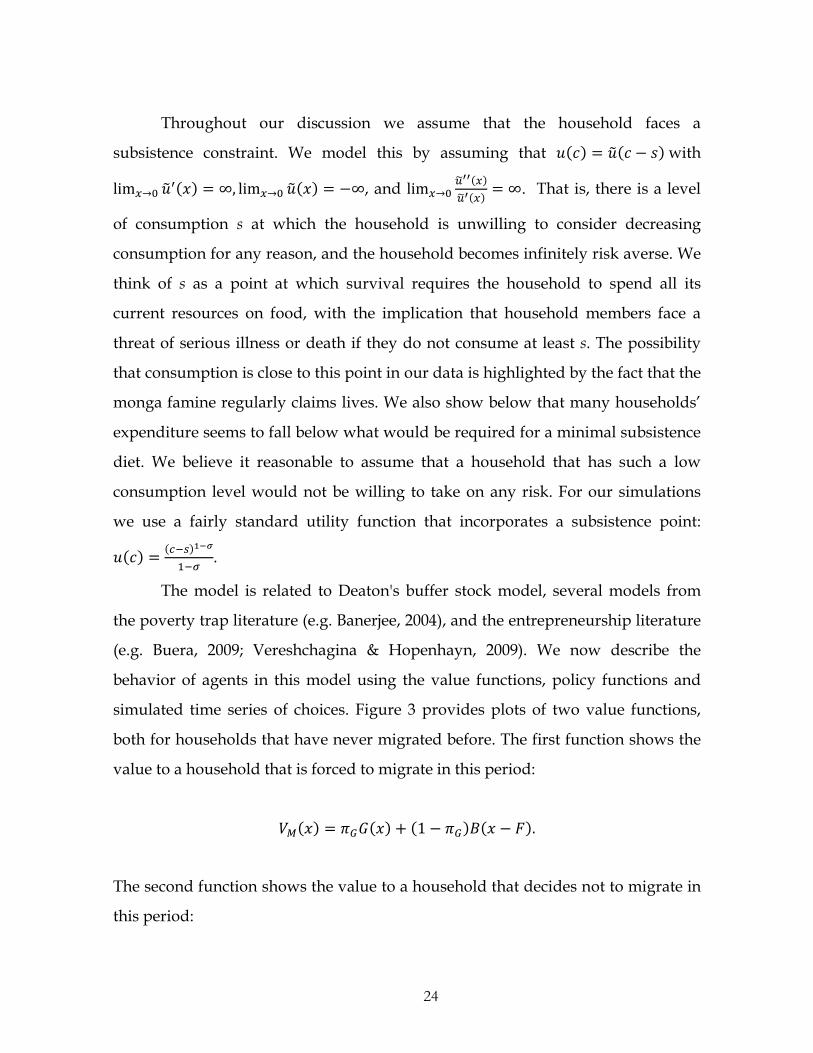
simulated time series of choices. Figure 3 provides plots of two value functions,
both for households that have never migrated before. The first function shows the
value to a household that is forced to migrate in this period:
𝑉𝑀(𝑥) = 𝜋𝐺𝐺(𝑥) + (1 − 𝜋𝐺)𝐵(𝑥 − 𝐹).
The second function shows the value to a household that decides not to migrate in
this period:
24
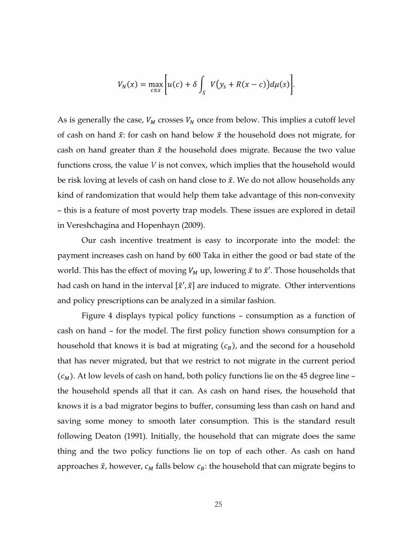
𝑉𝑁(𝑥) = max𝑐≤𝑥
�𝑢(𝑐) + 𝛿 � 𝑉�𝑦𝑠 + 𝑅(𝑥 − 𝑐)�𝑑𝜇(𝑠)𝑆
�.
As is generally the case, 𝑉𝑀 crosses 𝑉𝑁 once from below. This implies a cutoff level
of cash on hand 𝑥�: for cash on hand below 𝑥� the household does not migrate, for
cash on hand greater than 𝑥� the household does migrate. Because the two value
functions cross, the value V is not convex, which implies that the household would
be risk loving at levels of cash on hand close to 𝑥�. We do not allow households any
kind of randomization that would help them take advantage of this non-convexity
– this is a feature of most poverty trap models. These issues are explored in detail
in Vereshchagina and Hopenhayn (2009).
Our cash incentive treatment is easy to incorporate into the model: the
payment increases cash on hand by 600 Taka in either the good or bad state of the
world. This has the effect of moving 𝑉𝑀 up, lowering 𝑥� to 𝑥�′. Those households that
had cash on hand in the interval [𝑥�′, 𝑥�] are induced to migrate. Other interventions
and policy prescriptions can be analyzed in a similar fashion.
Figure 4 displays typical policy functions – consumption as a function of
cash on hand – for the model. The first policy function shows consumption for a
household that knows it is bad at migrating (𝑐𝐵), and the second for a household
that has never migrated, but that we restrict to not migrate in the current period
(𝑐𝑀). At low levels of cash on hand, both policy functions lie on the 45 degree line –
the household spends all that it can. As cash on hand rises, the household that
knows it is a bad migrator begins to buffer, consuming less than cash on hand and
saving some money to smooth later consumption. This is the standard result
following Deaton (1991). Initially, the household that can migrate does the same
thing and the two policy functions lie on top of each other. As cash on hand
approaches 𝑥�, however, 𝑐𝑀 falls below 𝑐𝐵: the household that can migrate begins to
25
save up for migration. Thus, the saving of a potential migrator can be divided into
two parts: buffering, and saving up for migration. The figure shows that, for some
parameter values, consumption is not a monotone function of cash on hand, a
result that is consistent with the findings of Buera (2009). As cash on hand rises
past 𝑥�, 𝑐𝑀 continues to lie below 𝑐𝐵: we have constrained the household not to
migrate in this period so it continues to save in the hope of migrating next period.
Finally, there is a level of cash on hand past which 𝑐𝑀 > 𝑐𝐵 – the household that
has never migrated knows that it can migrate next period and it is consequently
richer (in expectation) than the household that knows it is bad at migrating.
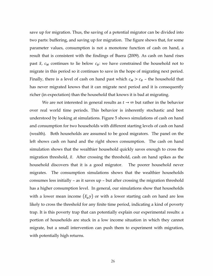
We are not interested in general results as 𝑡 → ∞ but rather in the behavior
over real world time periods. This behavior is inherently stochastic and best
understood by looking at simulations. Figure 5 shows simulations of cash on hand
and consumption for two households with different starting levels of cash on hand
(wealth). Both households are assumed to be good migrators. The panel on the
left shows cash on hand and the right shows consumption. The cash on hand
simulation shows that the wealthier household quickly saves enough to cross the
migration threshold, 𝑥�. After crossing the threshold, cash on hand spikes as the
household discovers that it is a good migrator. The poorer household never
migrates. The consumption simulations shows that the wealthier households
consumes less initially – as it saves up – but after crossing the migration threshold
has a higher consumption level. In general, our simulations show that households
with a lower mean income �𝐸𝜇𝑦� or with a lower starting cash on hand are less
likely to cross the threshold for any finite time period, indicating a kind of poverty
trap. It is this poverty trap that can potentially explain our experimental results: a
portion of households are stuck in a low income situation in which they cannot
migrate, but a small intervention can push them to experiment with migration,
with potentially high returns.
26

We can also use the model to consider other comparative statics. Risk
aversion appears intuitively linked to aversion to experimentation, but the model
suggests that the relationship is more complicated. Simulations show that an
increase in risk aversion has three effects. First, increasing risk aversion increases
the cost of experimenting with migration and tends to increase 𝑥� and thus reduce
the propensity to migrate. Second, as risk aversion increases, the return to
migration increases because migration can be seen as a risk mitigation strategy.
Third, for many utility functions (including the one we use for simulations),
absolute prudence increases with risk aversion.21 As a consequence, as risk
aversion increases the household engages in more buffer stock saving, implying
that the household is more likely to cross any given threshold level of cash on
hand. We have not sought a general characterization of which effect dominates,
but do observe all three effects in our simulations. Similar effects apply to an
increase in the riskiness of income. On the one hand a riskier income means more
background risk and, therefore (for specific utility functions) effectively an increase
in risk aversion. On the other hand, more risk means more buffer stock savings.
6 Qualitative Evaluation of the Model’s Assumptions and Central Implications
In this section we provide some descriptive and some experimental evidence in
favor of the main assumptions and implications of the model.
6.1 Descriptive Evidence on Income Variability and Buffering
A key assumption of the model is that the income process is stochastic. To verify
whether this describes our setting, we study the inter-temporal variability in the
21 The coefficient of absolute prudence is defined as 𝑢′′′(𝑥)𝑢′′(𝑥) . See Kimball (1990) for a definition of prudence
and the relationship to precautionary savings and concepts of risk aversion including decreasing absolute risk aversion.
27

three rounds of consumption data collected at baseline (July 2008), December 2008
and December 2009. We conservatively use consumption data rather than income
data because income is measured with more error in these settings (Deaton, 1997)
and this would artificially inflate variability, and because income is more variable
due to seasonality and consumption smoothing.
Even with the conservative measure, we see that average variability in per-
capita consumption is high. Mean absolute deviation in weekly consumption in
our sample is 307 Taka between rounds one and two and 368 Taka between rounds
two and three. The standard deviation of the absolute deviation in income is 635
and 508 Taka respectively. By way of comparison, average per-capita consumption
levels in the control group were 1067, 954 and 1227 Taka in the three surveys. In
Appendix Figure 1 we plot histograms of second round consumption separately
for each of the 10 deciles of first round household consumption. Visual inspection
suggests that there is no real permanence in the income distribution - those that
were in the lowest decile in the first round do not appear to have a significantly
different draw in the second period from those that were in the middle decile. We
verify this by regressing consumption in later rounds on in earlier rounds
consumption in Appendix Table 5. Every extra dollar of consumption measured in
July 2008 is associated with only 10.2 cents extra consumption in December 2008,
and 6.7 cents in December 2009. One dollar extra in December 2008 is associated
with 45 cents more consumption in December 2009. The R-squared in these
regressions are between 0.02-0.13: current consumption does not predict future
consumption well. Although measurement error is probably very important in
explaining these results, we think it is reasonable to conclude that background
income is also very variable.
The reported yearly variation in income and consumption dwarfs the size of
our 600 Taka incentive, and thereby poses a significant challenge to the model’s
ability to rationalize the data. Our model suggests a cutoff point of cash on hand
28
that would trigger migration. Our incentive presumably works, in part, by
increasing cash on hand. But, the data suggests that income (and, therefore, cash
on hand) will be higher by the size of the incentive regularly, just by pure chance.
This fact is primarily why we do not think that a pure liquidity constraint – the
complete inability to raise the bus fare – provides a good description of the setting.
We return to this issue below.
Background risk also has important implications for behavior. If
households are prudent (i.e. 𝑢′′′ > 0) and impatient (𝛿 > 𝑅), both of which seem
likely in our setting,22 then high income-variability should lead to buffer stock
savings. Appendix Table 6 describes savings behavior in our sample. Although
our households are poor, they have a reasonably high level of savings. Conditional
on being a saver, the mean holding in cash is 1400 Taka, which is about 35% of
monthly expenditure for the household. This is a relatively high
savings/expenditure ratio, even compared to the United States. For the full
sample (not conditioning on people with positive savings), average cash savings is
745 Taka, and average value of cash plus other liquid assets (e.g. jewelry and
financial assets) held by all households is 1085 Taka. This level of savings is not
inconsistent with the observation that households in our sample are often close to
subsistence. Buffering implies that in each period some households will have zero
savings and be consuming hand to mouth, but those same households will have
high savings in other periods. Indeed, the data bears this out quite well. 53% of
households held cash savings at baseline, and this fraction varies a lot across
rounds (57% in December 2008 and 34% in June 2011). The share of households
holding liquid assets varies from 42% to 59% to 81%. The standard deviation of
savings is also about two times mean savings which is consistent with savings
being variable, as it would be in a buffer stock model.
22 The existence of savings constraints in developing countries (Dupas & Robinson, 2013a) makes 𝛿 > 𝑅 reasonable. There are by now many theoretical and empirical arguments suggesting that prudence is a reasonable assumption for the utility function.
29
6.2 Descriptive and Experimental Evidence on Migration Risk
Our model assumes both that migration is risky, and that risk takes a particular
form: risk is assumed to be idiosyncratic. We begin by discussing evidence on
migration risk, and will turn to the specific form of the risk in Sections 6.3 and 6.4.
Figure 6 provides a clear depiction of the migration risk. We take the
monthly consumption per household member in December 2008, and subtract the
value of the incentive from households that chose to take it. This gives a measure
of the possible outcome if the cost of migration had to be born within one month
by the household, not subsidized by our incentive program. In panel A, we
subtract the histogram for distribution of consumption in the control (non-
incentive) villages from this histogram for the distribution of consumption in the
treatment (incentive) villages, less the value of the migration incentive paid out.
The results show significant amounts of risk: while the treatment moved many
poor households from extreme poverty (consuming 500-900 Taka per month) to a
less poor (1300 Taka per month) category, many other households would shift to
100-300 Taka per month (which, as discussed below, corresponds to caloric intake
at or below subsistence) without the payment to migrate. Panel B shows that the
risk disappears when we account for the program’s migration incentive payment
for those who took the money. This suggests that households at greatest risk were
the ones induced to migrate by our incentive, a result we will explore more
precisely below by creating a measure of subsistence.
6.2.1 Experiments on Migration Insurance
Motivated by our first two years of findings and the model, we also designed a
new experiment to directly test whether households perceive migration to be risky.
We returned to our sample villages in 2011 and offered a new set of treatments.
Appendix 2 describes the sampling frame and intervention design. To study risk,
30

the specific treatment was to offer a 800 Taka loan up-front conditional on
migration, but the loan repayment requirement is explicitly conditional on
measured rainfall conditions. Excessive rainfall is an important external event that
adversely affects labor demand and work opportunities at the destination. Rain
makes it more difficult to engage in skilled wage work at outdoor construction
sites (e.g. breaking bricks), it both increases the cost of pulling rickshaws and lower
the demand for a rickshaw transport. In terms of the model above, we think of
high rainfall as reducing the likelihood of finding a connection at the destination
(because job opportunities that allow you to display your skills to a potential
employer are scarce), as well as reducing the return to migration, m.
Appendix 3 develops a simple model of index insurance with basis risk to
clarify how this treatment is linked to household perceptions of migration risk.
Following Clarke (2011), we formalize basis risk as the probability that income is
low, but that rainfall is also low, so that the insurance does not pay out. In terms of
the above model, this would be the event of not finding a job connection during
your search (i.e. finding out you are a bad migrator) but still being forced to repay
the loan. Appendix 3 shows that our formalization implies that the portion of
people induced to migrate by the index insurance is decreasing in basis risk, if and
only if migration is risky and households are risky averse. We assume that
households that migrate to Bogra face lower basis risk, and farmers, for whom
high rainfall is usually beneficial, face greater basis risk.23
Table 7 shows results of regressing the 2011 migration rate on our 2011
treatments, and interactions of the insurance treatment with an indicator for
previous migration to Bogra, and an indicator for farmers. Column (1) shows that
the rainfall insurance contract induced migration, and that the effect is similar in
size as the effect of the simple (conditional) credit contract. Columns (2) and (3)
23 We use the basis risk variation to test for riskiness because our insurance is valuable even without risk, because also includes a credit element.
31
show that those with a propensity to travel to Bogra (i.e. lower basis risk) are more
affected by the insurance, while farmers (greater basis risk) find the insurance
contract less appealing. The farmer-insurance interaction is statistically significant
with 99% confidence, but the Bogra interaction is not significant at conventional
levels. Finally, column (4) shows that when we control for farmers, the Bogra
effect is much stronger (p-value of 0.15). For non-farming households who had a
preference for Bogra, the rainfall insurance contract induces 45% more migration in
2011. We see this set of results as reasonable strong evidence in favor of our
assumption that migration is risky, and households behave as though they are risk
averse.
6.3 Learning and Idiosyncratic Risk
Our model makes the assumption that migration risk takes a specific form: that it
is individual-specific (idiosyncractic), and resolved after one period of migration
(i.e, there is something to learn, or a connection to make.). Our motivation for
making this assumption is the strong and consistent repeat migration seen in the
data – half of all induced migrants migrate again, and this number is stable over 3
years. This result is very hard to drive without learning or accumulation of a
connection. Even if households earn a very large return on the investment F, the
impact will dissipate quickly because of the variability in base income.
6.3.1 Is Risk Idiosyncratic in this Setting?
We first examine whether migration risk is idiosyncratic, and try to identify the
nature of the risk from our data, before turning to evidence on learning. Our
information intervention – which provided general information on wages and the
likelihood of finding a job – has a precisely estimated zero impact on migration
rates. This is consistent with the assumption that risk is idiosyncratic, but may also
reflect the fact that this kind of information is not credible.
32
We next examine the determinants of 2009 re-migration to study directly
whether households are able to learn from others. As discussed above, our 2008
experiments contained several sub-treatments where additional conditions were
imposed: some households were required to migrate to specific destinations, some
were required to form groups, etc. This variation is within village and implies that
we have exogenous variation in the number of a household’s friends that migrated.
We also collected data at baseline on social relationships between all our sample
households to identify friends and relatives within the village. To test for learning
we run regressions of the form
𝑦𝑖 = 𝛼 + 𝛽𝑀𝑖 + 𝛾𝐹𝑖 + 𝜖𝑖
where 𝑦𝑖 is an indicator for second round migration, 𝑀𝑖 is an indicator for first
round migration and 𝐹𝑖 is a measure of how many of a household’s friends
migrated. We instrument 𝑀𝑖 and 𝐹𝑖 with all our treatments (incentives and
conditions on the migrant, and incentives and conditions on his friends), and
report OLS and IV results in Table 8. If there is learning from others we expect to
see 𝛾� > 0, because of the strong positive returns to migration. Table 8 shows
strong persistence in own migration: that inducing migration in 2008 with the
randomized treatments leads those same induced migrants to re-migrate in 2009.
However, friends’ migration choices the previous year have no impact on 2009
migration decisions, and this is a reasonably precisely estimated zero effect. This
suggests that people learn from their own experience, but do not learn from the
experiences of others. This provides strong support for the assumption that risk is
idiosyncratic as implied by the model.
Why is learning so individual-specific? The 2011 follow-up survey provides
a strong hint: Of the 2011 migrants provided incentives in 2008, 60% report going
back to work for the same employer at the same destination. Appendix Table 7
shows that being treated in 2008 leads to a 5 percentage point greater likelihood of
re-migrating and working for the same employer. A likely source of uncertainty
33
in the returns to migration thus appears to be the (potential) employer’s
incomplete information about the characteristics of specific migrants – are they
reliable, honest, hard-working? The typical employer in Dhaka is a rickshaw
garage owner who has to trust a migrant with his valuable asset. Research in India
has documented that migrants sometimes abandon the rented rickshaws at the
train or bus station (Jain & Sood, 2012). This would make it difficult for migrants
to “learn” from other villagers to resolve the uncertainty.24
Furthermore, migrants who were provided incentives in 2008 and who
continue working for the same employer in 2011 are significantly more likely to
have formed a connection to that specific employer in 2008, when they were
originally induced to go. Specifically, treatment group migrants are 16% more
likely to report forming the job connection to their current (2011) employer in 2008
instead of 2007, relative to “regular” migrants in the control group.25 This is again
strongly suggestive that the migrants who were induced to migrate by our
treatments formed an asset (a connection to an employer) at the destination, which
continued to provide value three years later.
Finally, among households that migrated in 2008 (in both incentive and
control groups), we asked whether these households knew someone at the
destination, or whether they had a job lead at the destination. These measures can
be thought of as proxies for whether the household’s type has been revealed –
households that have a connection have already determined their status while
those that do not have not, or know that they are bad at migrating.26 Our model
implies that the incentive will only have an impact on those that do not know their
24 Friends and relatives could potentially vouch for each other with employers, but this need not be believed. Further, making such a referral could be quite costly, it may put the referrers own job in danger, or require the referrer to look after a new migrant, perhaps providing some risk sharing and sharing housing.
25 Appendix Table 8 shows the results of the t-tests. Results are statistically significant at conventional levels for the difference tests (e.g. 2007 vs 2008), but not for the difference-in-difference (e.g. 2007 vs 2008, treatment vs control) tests.
26 According to our model, those that have migrated and know they are bad should not be in this sample that is entirely made up of migrators.
34
status and so we expect to see more migrators without a connection in the
incentive group. Table 9 shows that migrants in the control group are much more
likely to know someone at the destination, and to have a job lead, than are those in
the incentive treatment. This suggests that our treatment induced migrants among
those that had not already determined their status, as implied by the model.
6.3.2 Evidence on Learning
The fact that learning should be destination specific – a connection in
Dhaka, for example, is not useful when migrating to Bogra – allows us to test more
directly for learning effects using experimental variation induced by our
treatments. One of our treatments assigned a specific destination city (Bogra,
Dhaka, Munshigonj or Tangail) as a condition of receiving the migration incentive,
and creates exogenous variation in the destination choices in 2008. Learning or
creating a job connection implies that migrants assigned to a specific location
should be more likely to return to that particular location in 2009 than to any other.
Let 𝐷𝑖 be an indicator taking value 1 if household i migrated to destination
D in 2009, and 𝐷𝑖08 be an indicator taking value 1 if household i migrated to
destination D in 2008. We run regressions of the form
𝐷𝑖 = 𝛼 + 𝛽𝐷𝑖08 + 𝜖𝑖
for each of four destinations. The 2008 migration destination choice is
instrumented with the location randomly assigned to the household:
𝐷𝑖08 = 𝜆 + 𝜌𝑇𝐷𝑖08 + 𝜂𝑖 ,
where 𝑇𝐷𝑖08 is an indicator taking on value one if the households was assigned to
location D in 2008. Appendix Table 9 shows these first stage estimates to establish
that initial destination assignment had a strong effect on destination choices in
2008. The hypothesis of destination specific learning implies that there should be
more than one significant coefficient in the second stage estimates displayed in
35

Table 10.27 We see that all coefficients, instrumented with our location
requirements, are positive and that two are significant at the 10% level (Dhaka and
Munshigonj). The coefficients also imply quantitatively important stickiness.
Households randomly assigned to migrate to Munshigonj in 2008 are 30% more
likely to re-migrate to Munshigonj in 2009 than to any other location. We take this
as evidence in favour of location specific learning or the accumulation of
connections at the destination as being an important driver of migration behavior.
Our model also suggests that some induced migrants should discover that
they are bad migrators, while some discover that they are good. Among regular
migrants, however, our model predicts no such effects – only households that
know they are good at migrating should migrate in the control group. Figure 7
shows evidence consistent with this. In the treatment groups (credit or cash) those
that chose to re-migrate in 2009 had a significantly better migration experience in
2008 than those who chose not to re-migrate. In the control group, however, we
see no such effect.
6.4 Subsistence
Our model postulates that households may not migrate because they are
close to subsistence, and risk falling below subsistence if they have a bad migration
outcome. We can study the distribution of expenditures and caloric intake to
examine whether this setup is warranted.
The Bangladesh Bureau of Statistics classifies a person as ultra-poor if they
consume less than 1605 calories, and it is usually thought that something between
27 There may be inherent differences in profitability of each location, and just showing that those assigned to migrate to Dhaka are more likely than others to re-migrate to Dhaka is consistent with Dhaka simply being the most profitable place to migrate, and re-migration simply reflecting initial success. We overcome this issue by observing that only one destination can be the most profitable, and examining re-migration propensities for all 4 of our assigned destination. We will need to show that migration assignment leads to destination-specific re-migration to at least two different cities. Note that location specific learning does not imply that all regressions would have positive coefficients -- some locations may just be really bad placed to migrate.
36

600 and 1000 calories are required just to survive. Based on the prices collected in
our baseline survey, and assuming very basic calorie composition, we estimate that
it would cost about 660 Taka per person per month to meet the ultra-poor level,
450 taka to consume 1000 calories and 250 Taka to consume 600 calories.
Comparing these figures to the distribution of per-capita expenditures in our
sample presented in Appendix Figure 1, we see that a substantial portion of
households are close to subsistence. Appendix Figure 2 shows directly the
histogram of calories per person per day in the control group in our December
2008 follow-up. Many households in the control group can be characterized as
“close to subsistence” in terms of caloric intake. Comparing the treatment and
control histograms, we again see that our treatment moved many people from a
subsistence level of consumption (of 800-1300 calories per person per day) to a
comfortable level exceeding 2000 calories per person per day.
Our model suggests that if aversion to the risk of falling below subsistence
is an important deterrent to migration, then: (a) people close to subsistence should
not be migrating in the control group, and (b) our treatment should have the
largest effect on households that are close to subsistence: they should be the ones
induced to migrate by our incentive. The three panels in Figure 8 show strong
evidence in favor of these two claims graphically and in a regression. We measure
subsistence as the proportion of total household expenditures devoted to food. The
regression and the graphs show that those closer to subsistence are significantly
less likely to migrate in the control group, and their migration decisions respond
most strongly to the treatment.
6.5 Does the Model Rationalize Responses to all Treatments?
The model allows us to understand the impact of specific treatments designed to
help households accumulate sufficient cash on hand to engage in profitable
37

migration. In this section we compare the impacts of several potential policies on
which we have collected data.
First, as noted above our initial treatments included both a cash and a credit
incentive. In practice these two incentives have approximately the same impact on
the migration rate. Here we argue that this finding is consistent with the model, if
credit is seen as incorporating a limited liability aspect. An assumption of limited
liability is consistent with the fact that only 80% of households repaid the loan.
We can capture the limited liability effect of credit by noting that
households have to have a reason to repay their loans. Let 𝑀(𝑥) = 𝐵(𝑥 − 𝐹) if the
household is a bad migrator a 𝑀(𝑥) = 𝐺(𝑥) if the houshold is a good migrator, and
consider a household that has a loan of value L and is required to repay Z. The
household will repay the loan iff
𝑀(𝑥 − 𝑍) ≥ 𝑀(𝑥 + 𝐿) − 𝑃,
where P is a utility cost of punishment by the lender. P is assumed to be state
independent as the punishment should reflect the long run value of credit to the
household. With this formulation there is 𝑥�𝐵 and 𝑥�𝐺 such that the loan will be
repaid by a bad migrator if 𝑥 ≥ 𝑥�𝐵and by a good migrator if 𝑥 ≥ 𝑥�𝐺 . It is easy to
show that 𝑥�𝐵 < 𝑥�𝐺 and that a bad migrator will always default on the loan if the
cost of migration, F, is large enough. Further, because utility becomes infinitely
negative when consumption approaches subsistence, to a first approximation,
𝑀(𝑥�𝐵 + 𝐿) ≈ 𝑀(𝑥�𝐵 + 𝐿) − 𝑃 for a bad migrator for whom 𝑥 − 𝐹 is close to
subsistence. This implies that the utility cost P need not have a large impact on the
ability of the credit contract to provide insurance.
To incorporate these observations into the above model, assume that
𝑥�𝐵 < 𝑥� < 𝑥�𝐺 . This assumption implies that a first time migrator that discovers it is
a bad migrator will not repay the loan, but a first time migrator that is good, will
38
repay the loan. As discussed above, the decision to migrate is determined by the
intersection between the curves 𝑉𝑀 and 𝑉𝑁, if 𝐵′(𝑥�) is large and positive and 𝐺′(𝑥�)
is small, then the impact of credit and cash will be, approximately, the same.
Consequently, the model can capture the idea that credit and cash will have the
same impact. Obviously from a policy perspective, credit is a much less costly
intervention. Interpreted in the light of this analysis, the fact that credit and cash
treatments have a similar impact on migration rates again suggests that risk, which
is mitigated by the limited liability aspect of the loan, is important in explaining
our data.
Second, as noted above, we returned in 2011 and implemented new
treatments. One of these treatments was an unconditional credit contract of the
same size at the conditional credit transfer. Our motivation for this experiment was
to rule out the possibility that households were merely cash constrained. Our
model implies that the credit incentive should have a larger impact as it moves
only the 𝑉𝑀 curve, while the unconditional credit raises the 𝑉𝑁 curve as well. This
is an implication of any model in which a household weighs the returns to
migration relative to other possible uses of the money, but is not an implication of
a model where the household knows that migration is profitable, but simply
cannot afford it. The results of this experiment are shown in Table 7, and show
that, consistent with our model but inconsistent with the cash constraint model, the
unconditional transfer has a smaller impact than the conditional transfer.28
6.6 Summary of Qualitative Tests
In summary, both descriptive and experimental analyses of the data indicate
that our model accurately captures many key aspects of the environment:
background income is volatile, migration is risky, savings is high and migration is
28 Although we presented the products in a similar way, if household perceptions of repayment requirements varied between the conditional and unconditional loans, that may also lead to differential take-up.
39

an experience good. The model also rationalizes most of the data coming from our
experiment: the fact that credit and cash have similar sized impacts, the fact that
the incentive was most effective for those that are close to subsistence, the relative
impacts of unconditional and conditional transfers, and the response to the
insurance treatment. What remains to be seen, however, is whether the model
brings all of these ingredients of the migration decision together in a way that can
quantitatively account for the magnitude of the experimental effects.
7 Quantitative Calibration of the Model
Our quantitative exercise will use the data to calibrate all the free parameters
of the model except risk aversion. We then ask what level of risk aversion would
be required to match key aspects of the data. Table 11 shows the parameters we
use for the quantitative exercise. In all cases we have erred on the side of allowing
the model to generate the experimental estimates. This choice reflects the fact that
we will ultimately argue that the model in its basic form is not able to rationalize
the experimental estimates.
Three choices deserve special mention. First, we assume that there are two
opportunities to migrate each year (or two time periods per year): one after each
planting season. This means that a time period for the purpose of the model
should be thought of as half a year. Second, we assume that the cost of migration,
F, must be borne over 1 month, so that consumption when migration is bad is very
low. This reflects the fact that most households earn money during the monga
season and use it to pay for consumption. Credit constrained households will have
to pay for migration out of this income. This choice is obviously quite extreme but
could be justified by arguing that the extremely low consumption for a one-month
period would have a large effect on utility relative to the remaining months in the
monga period with a higher consumption level. Third, we assume that income at
40
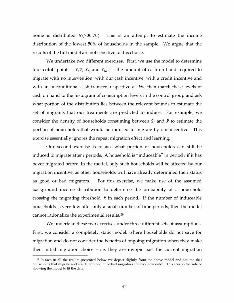
home is distributed 𝑁(700,70). This is an attempt to estimate the income
distribution of the lowest 50% of households in the sample. We argue that the
results of the full model are not sensitive to this choice.
We undertake two different exercises. First, we use the model to determine
four cutoff points – 𝑥�, 𝑥�𝐼 , 𝑥�𝐶 and 𝑥�𝑈𝐶𝑇 – the amount of cash on hand required to
migrate with no intervention, with our cash incentive, with a credit incentive and
with an unconditional cash transfer, respectively. We then match these levels of
cash on hand to the histogram of consumption levels in the control group and ask
what portion of the distribution lies between the relevant bounds to estimate the
set of migrants that our treatments are predicted to induce. For example, we
consider the density of households consuming between 𝑥𝐼� and 𝑥� to estimate the
portion of households that would be induced to migrate by our incentive. This
exercise essentially ignores the repeat migration effect and learning.
Our second exercise is to ask what portion of households can still be
induced to migrate after t periods. A household is “induceable” in period t if it has
never migrated before. In the model, only such households will be affected by our
migration incentive, as other households will have already determined their status
as good or bad migrators. For this exercise, we make use of the assumed
background income distribution to determine the probability of a household
crossing the migrating threshold 𝑥� in each period. If the number of induceable
households is very low after only a small number of time periods, then the model
cannot rationalize the experimental results.29
We undertake these two exercises under three different sets of assumptions.
First, we consider a completely static model, where households do not save for
migration and do not consider the benefits of ongoing migration when they make
their initial migration choice – i.e. they are myopic past the current migration
29 In fact, in all the results presented below we depart slightly from the above model and assume that households that migrate and are determined to be bad migrators are also induceable. This errs on the side of allowing the model to fit the data.
41
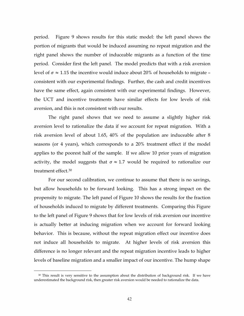
period. Figure 9 shows results for this static model: the left panel shows the
portion of migrants that would be induced assuming no repeat migration and the
right panel shows the number of induceable migrants as a function of the time
period. Consider first the left panel. The model predicts that with a risk aversion
level of 𝜎 ≈ 1.15 the incentive would induce about 20% of households to migrate –
consistent with our experimental findings. Further, the cash and credit incentives
have the same effect, again consistent with our experimental findings. However,
the UCT and incentive treatments have similar effects for low levels of risk
aversion, and this is not consistent with our results.
The right panel shows that we need to assume a slightly higher risk
aversion level to rationalize the data if we account for repeat migration. With a
risk aversion level of about 1.65, 40% of the population are induceable after 8
seasons (or 4 years), which corresponds to a 20% treatment effect if the model
applies to the poorest half of the sample. If we allow 10 prior years of migration
activity, the model suggests that 𝜎 ≈ 1.7 would be required to rationalize our
treatment effect.30
For our second calibration, we continue to assume that there is no savings,
but allow households to be forward looking. This has a strong impact on the
propensity to migrate. The left panel of Figure 10 shows the results for the fraction
of households induced to migrate by different treatments. Comparing this Figure
to the left panel of Figure 9 shows that for low levels of risk aversion our incentive
is actually better at inducing migration when we account for forward looking
behavior. This is because, without the repeat migration effect our incentive does
not induce all households to migrate. At higher levels of risk aversion this
difference is no longer relevant and the repeat migration incentive leads to higher
levels of baseline migration and a smaller impact of our incentive. The hump shape
30 This result is very sensitive to the assumption about the distribution of background risk. If we have underestimated the background risk, then greater risk aversion would be needed to rationalize the data.
42

occurs because, as risk aversion increases, the value of migration as a risk
mitigation activity increases. The figure shows that at some point this effect
dominates the other impact of risk aversion, which is to make experimenting with
migration less tolerable. The figure suggests that a risk aversion level of 1 is
required to rationalize the data if we do not consider the repeat migration effect.
The right panel of Figure 10 shows the fraction of induceable migrants when
households are forward looking, but cannot save up. The hump in the portion of
induced migrants in the left panel implies that we need not consider risk aversion
levels above about 7 – as 𝜎 increases past this point risk aversion in fact reduces the
propensity to migrate.31 After 4 years, 40% of the sample will be induceable if risk
aversion is as high as 5. If we consider longer time horizons such as 10 years, then
the figure implies that no level of risk aversion is high enough to allow for a large
number of induceable migrants.
The results in Figure 10 may, however, overestimate the importance of
migration. Because we do not allow savings, households are unable to buffer, and
the value of migration as a risk mitigation strategy is increased. Figure 11 shows
the results for the full model, where we allow for both buffer stock savings, and for
the agent to save up for migration. The left panel confirms the intuition that
savings reduces the value of migration. The right hand panel, however, shows
that the ability to save up dominates: once we allow for savings we would need a
risk aversion of 11.5 to replicate our treatment effects allowing 4 years of migration
activity, and if we allow 10 years of migration activity, even a risk aversion level of
20 is insufficient to rationalize the results.32
31 The hump in the left panel is based on the empirical distribution of consumption levels. For the simulations shown in the right panel we make use of our assumed distribution which leads to a maximal effect of the incentive at a risk aversion level of 7.
32 These results assume that households begin time with no assets and the lowest possible income shock. We use the model to generate policy functions as well as cutoff values. We then simulate the model for 10,000 households and ask what portion of those 10000 households have not migrated after t periods.
43

The results allowing for savings suggest a sense in which our main
conclusions are robust to our assumption regarding the distribution of income. We
have simulated the right panel of Figure 11 for standard deviations in from 40 to
140 and the results are almost identical. As discussed above there are several
impacts of increasing the degree of background risk, and the simulations suggest
that, given our calibrations, these effects cancel each other out.
We can also use the full model to ask whether the observed level of savings
is consistent with the model. For a risk aversion level of 0.5 the model predicts a
household will hold, on average 1500 Taka in savings, which is roughly in line
with what we see in the data. For higher levels of risk aversion, however, the
model predicts far more savings than we observe: at a risk aversion level of 5,
predicted average savings is close to 3000 Taka and at 𝜎 = 10 we predict savings of
nearly 5000 Taka. It is not possible to match both the level of savings and the
responses to the migration treatments at any given level of assumed risk aversion.
8 Extensions
While the qualitative evaluation of the model had shown that households
do save, that they respond to migration incentives in ways predicted by the model,
and that they perceive migration to be risky, the calibration exercise suggests that
to match the magnitudes of responses and household behaviors, we have to extend
the model in some ways. It could be that households under-estimate the benefits
of migration, or they fail to actively save up for migration, or they are insufficiently
forward-looking. In this section we discuss extensions to our baseline model that
would allow us to better accommodate the data. In all cases, we do not have the
data to determine conclusively which extensions are the most important. We
therefore see this section more as an extended call for more work. We provide
some suggestive evidence from our data of approaches that are unlikely to work.
44
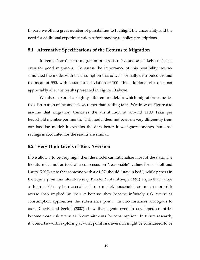
In part, we offer a great number of possibilities to highlight the uncertainty and the
need for additional experimentation before moving to policy prescriptions.
8.1 Alternative Specifications of the Returns to Migration
It seems clear that the migration process is risky, and m is likely stochastic
even for good migrators. To assess the importance of this possibility, we re-
simulated the model with the assumption that m was normally distributed around
the mean of 550, with a standard deviation of 100. This additional risk does not
appreciably alter the results presented in Figure 10 above.
We also explored a slightly different model, in which migration truncates
the distribution of income below, rather than adding to it. We draw on Figure 6 to
assume that migration truncates the distribution at around 1100 Taka per
household member per month. This model does not perform very differently from
our baseline model: it explains the data better if we ignore savings, but once
savings is accounted for the results are similar.
8.2 Very High Levels of Risk Aversion
If we allow σ to be very high, then the model can rationalize most of the data. The
literature has not arrived at a consensus on “reasonable” values for σ: Holt and
Laury (2002) state that someone with σ >1.37 should “stay in bed”, while papers in
the equity premium literature (e.g. Kandel & Stambaugh, 1991) argue that values
as high as 30 may be reasonable. In our model, households are much more risk
averse than implied by their 𝜎 because they become infinitely risk averse as
consumption approaches the subsistence point. In circumstances analogous to
ours, Chetty and Szeidl (2007) show that agents even in developed countries
become more risk averse with commitments for consumption. In future research,
it would be worth exploring at what point risk aversion might be considered to be
45
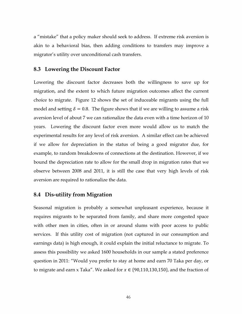
a “mistake” that a policy maker should seek to address. If extreme risk aversion is
akin to a behavioral bias, then adding conditions to transfers may improve a
migrator’s utility over unconditional cash transfers.
8.3 Lowering the Discount Factor
Lowering the discount factor decreases both the willingness to save up for
migration, and the extent to which future migration outcomes affect the current
choice to migrate. Figure 12 shows the set of induceable migrants using the full
model and setting 𝛿 = 0.8. The figure shows that if we are willing to assume a risk
aversion level of about 7 we can rationalize the data even with a time horizon of 10
years. Lowering the discount factor even more would allow us to match the
experimental results for any level of risk aversion. A similar effect can be achieved
if we allow for depreciation in the status of being a good migrator due, for
example, to random breakdowns of connections at the destination. However, if we
bound the depreciation rate to allow for the small drop in migration rates that we
observe between 2008 and 2011, it is still the case that very high levels of risk
aversion are required to rationalize the data.
8.4 Dis-utility from Migration
Seasonal migration is probably a somewhat unpleasant experience, because it
requires migrants to be separated from family, and share more congested space
with other men in cities, often in or around slums with poor access to public
services. If this utility cost of migration (not captured in our consumption and
earnings data) is high enough, it could explain the initial reluctance to migrate. To
assess this possibility we asked 1600 households in our sample a stated preference
question in 2011: “Would you prefer to stay at home and earn 70 Taka per day, or
to migrate and earn x Taka”. We asked for 𝑥 ∈ {90,110,130,150}, and the fraction of
46

respondents who stated they were willing to migrate were {58, 77, 83, 91}
respectively. Their responses imply that for every Taka increase in earnings per
day at the destination, migration probability increases by 0.5 percentage points.
Extrapolating, the respondents would have to be compensated Tk. 15,000 to induce
them to migrate for 75 days (which is the average length of migration).33 These
results suggest quite a high utility cost of migration.34 To incorporate these figures
into our quantitative analysis we take a very simple approach: we reduce the
return to migration to m/2 – an assumption consistent with 70 Taka at home being
worth 140 away, towards the high end of the answers we received. The results do
not change drastically in the full model (with savings) under this assumption.
Migration continues to be a good way to mitigate risk and households will want to
save up for it.
8.5 Incorrect Beliefs
In our calibration above we assumed that households were correct in their beliefs
about 𝜋𝐺, m and F. If households have incorrect beliefs then it would be much
easier to rationalize our empirical observations. Beliefs could be incorrect for two
conceptually distinct reasons. First, beliefs may be correct on average, but some
households have optimistic beliefs while others are pessimistic. In such a model
optimistic households would migrate and the pessimistic would not. Then non-
33 We also estimate this “demand curve for staying at home” with a revealed preference approach, using the fact that re-migration in 2009 was strongly responsive to migration earnings in 2008. That analysis suggests that re-migration probability increased by 1.7 percentage points for every 1000 Taka increases in migration earnings. Under some mild assumption, this implies that migrants induced by our treatment in 2008 would have to be compensated Tk. 21,700 to induce them to re-migrate in 2009.
34 Banerjee and Duflo (2007) arrive at a similar conclusion while describing the lives of the poor – “Why Don’t the Poor Migrate for Longer…given that they could easily earn much more by doing so?” “The ultimate reason seems to be that making more money is not a … large enough priority to experience several months of living alone and often sleeping on the ground somewhere in or around the work premises.”
47
migrators would appear to be systematically biased (Spinnewijn, 2012). Second, it
may be that beliefs are systematically pessimistic.35
To test whether biased beliefs are important, we asked all migrants in both
treatment and control groups about how their migration experience, in terms of
time it took to find work and their earnings at destination, compared to their
expectations prior to migration. For either interpretation of bias – systematic or on
average correct – we would expect that those in the control group, who were
already migrating and had had a chance to learn, would have roughly correct
beliefs, while those in the treatment group would have beliefs biased toward the
overly pessimistic.36 Results presented in Table 12 are not consistent with biased
beliefs: treatment group migrants do not have significantly different beliefs from
control group migrants.
8.6 Heterogeneity
Heterogeneity does not seem to be a particularly attractive way to accommodate
the data. For example, if we imagine that some households have a high m and
some a low m, this helps us to rationalize the lack of migration for the low m
households, but makes it even more difficult for the high m households.
8.7 Savings Constraints
The slightly different character of our results for the model with and without
savings points to the possible conclusion that it is savings behavior in our setting
that is the real anomaly (why are people not saving up to migrate?). Our sample
households may be savings-constrained due to sharing norms (Jakiela & Ozier,
35 This could be because non-migrators have access to incorrect information. McKenzie et al. (2007) argue that migrant households provide incorrect information because they do not want to have to share resources, or job connections and accommodation at the destination.
36 To be clear, it is not evidence of incorrect beliefs that some people found the experience worse than anticipated, this is perfectly consistent with an ex-post statement about an ex-ante risky event. The prediction of biased beliefs is that those in the treatment should be more likely to have done better than expected.
48
2012), or they may simply be no safe place to store things. This conclusion is
consistent with recent research that demonstrates very large impacts of simple
interventions that relax savings constraints (e.g. Dupas & Robinson, 2013b). Two
caveats should be mentioned, however. First, before citing savings constraints as
the key issue, it is necessary to understand why households are able to buffer, but
not to save up a lump-sum amount for migration. Second, the right panel of
Figure 10, in which we consider a forward looking household that cannot save,
suggest that there is a need to understand more than just savings constraints, we
must also understand why households act as though they are not aware of the full
benefits of migration.
Another related avenue to consider may be the need to share risk and solve
public goods problems in general. Risk sharing networks not only constrain
savings; they may also deter profitable investments (e.g. Lewis, 1955). Migrating
away may undermine network ties, and this may be a hidden cost of migration
(Munshi & Rosenzweig, 2009). We lack the data necessary to explore this channel.
8.8 Behavioral or Psychological Explanations
Many models that fall under the rubric of behavioral economics could be used to
explain the results. In this area we are particularly wary of making
pronouncements without data, as there are many different possible explanations of
this type. Here we mention just two models that have been applied to developing
country contexts. First, the quasi-hyperbolic discounting model of Laibson (1997)
can likely to applied to rationalize the data for some values of 𝛽. The version of
this model discussed in Duflo, Kremer and Robinson (2011) provides an
explanation for low savings. The version of this model discussed in Banerjee and
Mullainathan (2010) can explain why households do not undertake profitable
investments. Their model also suggests that commitment devices could be useful
49

policy interventions. Second, Koszegi and Rabin (2006)’s model of reference
dependence can likely rationalize the data. That model provides a non-self control
based explanation for the fact that household find themselves to be perpetually
without the money they need to invest: households adjust their expected
consumption in response to shocks and then assess the costs of investments
relative to this expected consumption level.
In summary, there are numerous avenues that could be pursued to get a
better quantitative accounting of the data generated by our experiment. We have
noted just a few. We are currently working on isolating which factors are most
relevant in other settings where seasonal migration is relevant.
9 Concluding Remarks
We conducted a randomized experiment in which we incentivized
households in a famine-prone region of Bangladesh to send a seasonal migrant to
an urban area. The main results show that a small incentive led to a large increase
in the number of seasonal migrants, that the migration was successful on average
(in terms of improving consumption by around 30%), and that households given
the incentive in one year continued to be more likely to migrate in future years.
These results bolster the case made by Clemens et al (2008), Rosenzweig (2006),
Gibson and McKenzie (2010), Clemens (2011), Rodrik (New York Times, 2007) and
Hanson (2009) that offering migration opportunities has large effects on welfare,
even relative to other promising development interventions in health, education,
trade or agriculture. The literature largely focuses on international migration, and
we show that the returns to internal migration – a much more common, but under-
studied phenomenon37 – are also large.
37 There were 240 times as many internal migrants in China in 2001 as there were international migrants (Ping, 2003), and 4.3 million people migrated internally in the 5 years leading up to the 1999 Vietnam census compared to only 300,000 international migrants (Anh, 2003).
50
We argue that the results are qualitatively consistent with a simple (rational)
model of a poverty trap where households that are close to subsistence face a small
possibility that migrating will turn out badly, leaving household consumption
below subsistence. The model helps us to understand the types of situation in
which we would expect incentive and insurance policies to lead to long-term
benefits as observed in our experiment. We should look for situations in which the
investment is risky, that risk is individual-specific, and where the utility cost of the
downside risk is large (e.g. the household is close to subsistence). These
predictions also provide an answer to the puzzle that motivated the entire project:
why does Rangpur – the poorest region of the country that regularly faces a
seasonal famine - have a lower out-migration rate compared to the rest of
Bangladesh? This can also explain other peculiar migration patterns noticed in the
literature – the lower out-migration rate among poorer Europeans (Hatton &
Williamson, 1998) and poorer South-Africans (Ardington et al., 2009).
Our quantitative work implies that we cannot provide a fully satisfying
explanation for why people in Rangpur had not saved up to migrate.38 We are
therefore hesitant to draw policy implications from our research. However, it is
clear that the migration support programs we implement help some Rangpur
households cope with the Monga famine, and appear more cost-effective than
subsidizing food purchases on an ongoing basis, which is the major anti-famine
policy tool currently employed by the Bangladesh government (Government of
Bangladesh 2005; Khandker et al., 2011). Two important caveats are that our
research does not capture long-term psychological and social effects of migration,
and the scale of our experiment does not permit us to analyze potential adverse
38 Several other papers document very high rates of return to small capital investments in developing countries (Udry & Anagol, 2006; de Mel et al., 2008; Bandiera et al., 2011; Duflo et al., 2011; Fafchamps et al., 2011), and this literature must also confront the same question of why households do not save to invest in these high-return activities.
51
general equilibrium effects in destination labor markets if the government were to
contemplate scaling up such a program.39
If there are net efficiency gains, this is likely because our intervention
mitigates the spatial mismatch between where people live, and where jobs are
during the pre-harvest months. This approach may be of relevance to other
countries that face geographic concentrations of poverty, such as northern Nigeria,
eastern islands of Indonesia, northeast India, southeast Mexico, and inland
southwest China (Jalan & Ravallion, 2001). More generally, providing credit to
enable households to search for jobs, and aid spatial and seasonal matching
between employers and employees may be a useful way to augment the
microcredit concept currently more narrowly focused on creating new
entrepreneurs and new businesses.40 The potential efficiency gains raise an
interesting question of why private sector entities do not profit by developing
mechanisms that link migrants to employers in the city. To understand this, we
interviewed several employers in Dhaka. The employers reported that there are in
fact “labor sardars” who bring migrant workers to Dhaka, but the process is
fraught with uncertainty and risk. Migrants have to be paid the one-way bus ticket
and some salary in advance, but it is difficult to enforce any long-term contract if
they disappear and choose to go work elsewhere after the transit cost is paid.
39 There is mixed evidence in the literature on whether these effects are substantial (Ottaviano & Peri, (forthcoming); Borjas, 2003; Borjas & Katz, 2007; Card, 2009). Moreover, general equilibrium effects may be positive in net, if spillover benefits at the origin exceed external costs at the destination. Migrants form a much larger part of the village economy at the origin compared to the destination urban economy.
40 With credit contracts, it may be difficult to collect regular repayment from migrants who move away, but one of the world’s largest micro-credit NGOs, BRAC, has recently introduced credit programs to finance even international migration.
52
References
Adams, Richard H. (1998). Remittances, Investment, and Rural Asset Accumulation in Pakistan. Economic Development and Cultural Change, 47(1): 155-173.
Akee, Randall. (2010). Who Leaves? Deciphering Immigrant Self-Selection from a Developing Country. Economic Development and Cultural Change, 58(2): 323-344.
Anh, Dang N. (2003). Migration and Poverty in Asia: With Reference to Bangladesh, China, the Philippines and Viet Nam. Conference proceedings: Ad Hoc Expert Group Meeting on Migration and Development, Organised by the Economic and Social Commission for Asia and the Pacific. Bangkok, 27–29 August:
Ardington, Cally, Case, Anne & Hosegood, Victoria. (2009). Labor Supply Responses to Large Social Transfers: Longitudinal Evidence from South Africa. American Economic Journal: Applied Economics, 1(1): 22-48.
Ashraf, Nava, Aycinena, Diego, Martinez, Claudia A. & Yang, Dean. (forthcoming). Remittances and the Problem of Control: A Field Experiment among Migrants from El Salvador. Review of Economics and Statistics
Aycinena, Diego, Martinez, Claudia A. & Yang, Dean. (2010). The Impact of Remittance Fees on Remittance Flows: Evidence from a Field Experiment among Salvadoran Migrants.
Bandiera, Oriana, Barankay, Iwan & Rasul, Imran. (2011). Field Experiments with Firms. Journal of Economic Perspectives, 25(3): 63-82.
Banerjee, Abhijit. (2004). The Two Poverties. In S. Dercon (Ed.), Insurance Against Poverty (pp. 59-76). Oxford: Oxford University Press.
Banerjee, Abhijit & Duflo, Esther. (2007). The Economic Lives of the Poor. Journal of Economic Perspectives, 21(1): 141-168.
Banerjee, Abhijit & Mullainathan, Sendhil. (2010). The Shape of Temptation: Implications for the Economic Lives of the Poor. Working Paper.
Banerjee, Abhijit & Newman, Andrew F. (1991). Risk-Bearing and the Theory of Income Distribution. The Review of Economic Studies, 58(2): pp. 211-235.
53
Bangladesh Bureau of Statistics. (2011). Monthly Statistical Bulletins. Retrieved from http://www.bbs.gov.bd/home.aspx
Barham, Bradford & Boucher, Stephen. (1998). Migration, Remittances, and Inequality: Estimating the Net Effects of Migration on Income Distribution. Journal of Development Economics, 55(2): 307-331.
Basu, Karna & Wong, Maisy. (2012). Evaluating Seasonal Food Security Programs in East Indonesia.
Beegle, Kathleen, De Weerdt, Joachim & Dercon, Stefan. (2011). Migration and Economic Mobility in Tanzania: Evidence from a Tracking Survey. The Review of Economics and Statistics, 93(3): 1010-33. doi:10.1162/REST_a_00105
Borjas, George. (2003). The Labor Demand Curve is Downward Sloping: Reexamining the Impact of Immigration on the Labor Market. The Quarterly Journal of Economics, 118(4): 1335-1374.
Borjas, George, & Katz, Lawrence. (2007). The Evolution of the Mexican-Born Workforce in the United States. In G. Borjas (Ed.), Mexican Immigration to the United States (pp. 13-55). Chicago, IL: University of Chicago Press.
Brown, Richard & Leeves, Gareth. (2007). Impacts of International Migration and Remittances on Source Country Household Incomes in Small Island States: Fiji and Tonga. Australia: School of Economics, The University of Queensland. Discussion Paper. No. 347.
Brune, Lasse, Gine, Xavier, Goldberg, Jessica & Yang, Dean. (2011). Commitments to Save: A Field Experiment in Rural Malawi. Washington, DC: The World Bank. Policy Research Working Paper. No. 5748.
Buera, Francisco J. (2009). A Dynamic Model of Entrepreneurship with Borrowing Constraints: Theory and Evidence. Annals of Finance, 5: 443-464. doi:10.1007/s10436-009-0121-2
Card, David. (2009). Immigration and Inequality. The American Economic Review, 99(2): 1-21. doi:10.1257/aer.99.2.1
Caselli, Francesco. (2005). Accounting for Cross-Country Income Differences. In P. Aghion, & S. Durlauf (Eds.), Handbook of Economic Growth (pp. 679-741). Amsterdam: Elsevier.
54
Chaudhuri, Shubham & Paxson, Christina. (2002). Smoothing Consumption Under Income Seasonality: Buffer Stocks Vs. Credit Markets Columbia University, Department of Economics. Department of Economics Discussion Papers. No. 0102-54. Retrieved from http://hdl.handle.net/10022/AC:P:363
Chetty, Raj & Szeidl, Adam. (2007). Consumption Commitments and Risk Preferences. The Quarterly Journal of Economics, 122(2): 831-877. doi:10.1162/qjec.122.2.831
Chin, Aimee, Karkoviata, Leonie & Wicox, Nathaniel. (2010). Impact of Bank Accounts on Migrant Savings and Remittances: Evidence from a Field Experiment. Universtiy of Houston. mimeo.
Clarke, Daniel J. (2011). A Theory of Rational Demand for Index Insurance. University of Oxford. Department of Economics Discussion Paper Series. No. 572. Retrieved from http://www.economics.ox.ac.uk/index.php/department-of-economics-discussion-paper-series/a-theory-of-rational-demand-for-index-insurance
Clemens, Michael. (2010). The Roots of Global Wage Gaps: Evidence from Randomized Processing of U.S. Visas. Washington, D.C.: Center for Global Development. No. Working Paper 212.
Clemens, Michael. (2011). Economics and Emigration: Trillion-Dollar Bills on the Sidewalk? The Journal of Economic Perspectives, 25(3): 83-106. doi:10.1257/jep.25.3.83
Clemens, Michael, Montenegro, Claudio E. & Pritchett, Lant. (2008). The Place Premium: Wage Differences for Identical Workers Across the U.S. Border. Washington, D.C.: Center for Global Development. No. Working Paper No. 148.
de Mel, Suresh, McKenzie, David & Woodruff, Christopher. (2008). Returns to Capital in Microenterprises: Results from a Randomized Experiment. Quarterly Journal of Economics, 123(4): 1329-1372.
Deaton, Angus. (1991). Savings and Liquidity Constraints. Econometrica, 59(5): 1221-1248.
Deaton, Angus. (1997). The Analysis of Household Surveys: A Microeconometric Approach to Development Policy. Baltimore: Johns Hopkins University Press for the World Bank.
55

Dercon, Stefan & Christiaensen, Luc. (2011). Consumption Risk, Technology Adoption and Poverty Traps: Evidence from Ethiopia. Journal of Development Economics, 96(2): 159-173.
Dercon, Stefan & Krishnan, Pramila. (2000). Vulnerability, Seasonality and Poverty in Ethiopia. Journal of Development Studies, 36(6): 25-53.
Dostie, B., Haggblade, S. & Randriamamonjy, J. (2002). Seasonal Poverty in Madagascar: Magnitude and Solutions. Food Policy, 27(5/6): 493.
Duflo, Esther, Kremer, Michael & Robinson, Jonathan. (2011). Nudging Farmers to use Fertilizer: Theory and Experimental Evidence from Kenya. The American Economic Review, 101(6): 2350-2390.
Dupas, Pascaline. (2010). Short-Run Subsidies and Long-Run Adoption of New Health Products: Evidence from a Field Experiment. National Bureau of Economic Research. No. 16298.
Dupas, Pascaline & Robinson, Jonathan. (2013a). Savings Constraints and Microenterprise Development: Evidence from a Field Experiment in Kenya. American Economic Journal: Applied Economics, 5(1): 163-192.
Dupas, Pascaline & Robinson, Jonathan. (2013b). Why Don't the Poor Save More? Evidence from Health Savings Experiments. American Economic Review, 103(4): 1138-1171. doi:10.1257/aer.103.4.1138
Eeckhoudt, Louis, Gollier, Christian & Schlesinger, Harris. (1996). Changes in Background Risk and Risk Taking Behavior. Econometrica, 64(3): 683-689. Retrieved from http://www.jstor.org/stable/2171866
Evenson, Robert E. & Gollin, Douglas. (2003). Assessing the Impact of the Green Revolution, 1960 to 2000. Science, 300: 758-762.
Fafchamps, Marcel, McKenzie, David, Quinn, Simon R. & Woodruff, Christopher. (2011). When is Capital enough to Get Female Microenterprises Growing? Evidence from a Randomized Experiment in Ghana. Washington, D.C.: National Bureau of Economic Research. Working Paper. No. 17207.
Fischer, Greg. (2013). Contract Structure, Risk Sharing and Investment Choice. Econometrica, 81(3): 883-939. doi:10.3982/ECTA9100
56
Foster, Andrew & Rosenzweig, Mark R. (2010). Microeconomics of Technology Adoption. Annual Review of Economics, 2(1): 395-424.
Foster, Andrew & Rosenzweig, Mark R. (2011). Are Indian Farms Too Small? Mechanization, Agency Costs and Farm Efficiency. Yale University: Working Paper.
Gibson, John & McKenzie, David. (2010). The Development Impact of a Best Practice Seasonal Worker Policy. Bureau for Research and Economic Analysis of Development. BREAD Working Paper. No. 286. Retrieved from http://ipl.econ.duke.edu/bread/abstract.php?paper=286
Gibson, John, McKenzie, David & Stillman, Steven. (2013). Accounting for Selectivity and Duration-Dependent Heterogeneity when Estimating the Impact of Emigration on Incomes and Poverty in Sending Areas. Economic Development and Cultural Change, 61(2): 247-280.
Gollin, Douglas, Lagakos, David & Waugh, Michael E. (2011). The Agricultural Productivity Gap in Developing Countries. New York University, Leonard N. Stern School of Business, Department of Economics. Working Paper Series. No. 11-14. Retrieved from https://files.nyu.edu/mw134/public/uploads/56836/apg.pdf
Gollin, Douglas, Parente, S. & Rogerson, R. (2002). The Role of Agriculture in Development. American Economic Review Papers and Proceedings, 92(2): 160-164.
Government of People’s Republic of Bangladesh. (2005). Bangladesh: Poverty Reduction Strategy Paper: Unlocking the Potential, National Strategy for Accelerated Poverty Reduction. Washington, D.C.: International Monetary Fund.
Grogger, Jeffrey & Hanson, Gordon H. (2011). Income Maximization and the Selection and Sorting of International Migrants. Journal of Development Economics, 95(1): 42-57.
Hanson, Gordon H. (2009). The Economic Consequences of the International Migration of Labor. Annual Review of Economics, 1: 179-207.
Hatton, Timothy & Williamson, Jeffrey. (1998). the Age of Mass Migration: An Economic Analysis New York: Oxford University Press.
Hausmann, Ricardo & Rodrik, Dani. (2003). Economic Development as Self-Discovery. Journal of Development Economics, 72(2): 603-633.
57

Holt, Charles A. & Laury, Susan K. (2002). Risk Aversion and Incentive Effects. The American Economic Review, 92(5): 1644-1655. Retrieved from http://www.jstor.org/stable/3083270
Jain, Tarun & Sood, Ashima. (2012). How does Relationship Based Governance Accomodate New Entrants? Evidence from the Cycle Rickshaw Rental Market.
Jakiela, Pamela & Ozier, Owen. (2012). Does Africa Need a Rotten Kin Theorem? Experimental Evidence from Village Economies. Working Paper.
Jalan, Jyotsna & Ravallion, Martin. (2001). Behavioral Responses to Risk in Rural China. Journal of Development Economics, 66(1): 23-49. doi:10.1016/S0304-3878(01)00154-7
Kanbur, Ravi. (1979). Of Risk Taking and the Personal Distribution of Income. Journal of Political Economy: 769-797.
Kandel, Shmuel & Stambaugh, Robert F. (1991). Asset Returns and Intertemporal Preferences. Journal of Monetary Economics, 27(1): 39-71. doi:10.1016/0304-3932(91)90004-8
Khandker, Shahidur R. (2012). Seasonality of Income and Poverty in Bangladesh. Journal of Development Economics, 97(2): 244-256. doi:http://dx.doi.org/10.1016/j.jdeveco.2011.05.001,
Khandker, Shahidur R., Khaleque, M. A. & Samad, Hussain. (2011). Can Social Safety Nets Alleviate Seasonal Deprivation? Evidence from Northwest Bangladesh. The World Bank. Policy Research Working Paper. No. 5865.
Khandker, Shahidur R. & Mahmud, Wahiduddin. (2012). Seasonal Hunger and Public Policies: Evidence from Northwest Bangladesh. Washington, D.C.: The World Bank.
Kihlstrom, Richard & Laffont, Jean-Jacques. (1979). A General Equilibrium Entrepreneurial Theory of Firm Formation Based on Risk Aversion. Journal of Political Economy, 87(4): 719-748.
Kimball, Miles S. (1990). Precautionary Saving in the Small and in the Large. Econometrica, 58(1): 53-73. Retrieved from http://www.jstor.org/stable/2938334
58
Koszegi, Botond & Rabin, Matthew. (2006). A Model of Reference-Dependent Preferences. The Quarterly Journal of Economics, 121(4): 1133-1165.
Kremer, Michael, Miguel, Edward, Mullainathan, Sendhil, Null, Clair & Zwane, Alix P. (2009). Making Water Safe: Price, Persuasion, Peers, Promoters, Or Product Design? Working Paper.
Laibson, David. (1997). Golden Eggs and Hyperbolic Discounting. Quarterly Journal of Economics, 113(2): 443-477.
Lewis, W. A. (1955). The Theory of Economic Growth. London: Allen & Unwin.
Macours, Karen & Vakis, Renos. (2010). Seasonal Migration and Early Childhood Development. World Development, 38(6): 857-869.
Martinez,Claudia A.,Yang,Dean. (2005). Remittances and Poverty in Migrants' Home Areas: Evidence from the Philippines. In C. Ozden, & M. Schiff (Eds.), International Migration, Remittances, and the Brain Drain (). Washington, D.C.: World Bank.
McKenzie, David. (2012). Learning about Migration through Experiments. Centre for Research and Analysis of Migration. CReAM Discussion Paper. No. 07/12. Retrieved from http://www.cream-migration.org/publ_uploads/CDP_07_12.pdf;
McKenzie, David, Gibson, John & Stillman, Steven. (2007). A Land of Milk and Honey with Streets Paved with Gold: Do Emigrants have Over-Optimistic Expectations about Incomes Abroad. The World Bank. Policy Research Working Paper. No. 4141. doi:10.1596/1813-9450-4141
McKenzie, David & Rapoport, Hillel. (2007). Network Effects and the Dynamics of Migration and Inequality: Theory and Evidence from Mexico. Journal of Development Economics, 84(1): 1-24.
McKenzie, David & Yang, Dean. (2010). Experimental Approaches in Migration Studies. Bonn: Institute for the Study of Labor (IZA). Discussion Paper. No. 5125.
McMillan, M. & Rodrik, Dani. (2011). Globalization, Structural Change and Productivity Growth. Cambridge, MA: NBER Working Paper. No. 17143.
59

Meredith, Jennifer, Robinson, Jonathan, Walker, Sarah & Wydick, Bruce. (2011). Keeping the Doctor Away: Experimental Evidence on Investment in Preventative Health Products. from http://people.ucsc.edu/~jmrtwo/HealthProducts.pdf
Miller, Grant & Mobarak, A. M. (2013). Gender Differences in Preferences, Intra-Household Externalities and Low Demand for Improved Cookstoves. Working paper. from http://faculty.som.yale.edu/mushfiqmobarak/stove_long.pdf
Munshi, Kaivan. (2004). Social Learning in a Heterogeneous Population: Technology Diffusion in the Indian Green Revolution. Journal of Development Economics, 73(1): 185-213.
Munshi, Kaivan & Rosenzweig, Mark R. (2009). Why is Mobility in India so Low? Social Insurance, Inequality, and Growth. National Bureau of Economic Research. No. Working Paper 14850.
Ottaviano, Gianmarco I. P. & Peri, Giovanni. ((forthcoming)). Rethinking the Effects of Immigration on Wages. Journal of the European Economic Association:
Paxson, Christina. (1993). Consumption and Income Seasonality in Thailand. Journal of Political Economy, 101(1): 39-72.
Ping, Huang (2003). China Migration Country Study. Conference proceedings: Regional Conference on Migration, Development and Pro-Poor Policy Choices in Asia. Dhaka, Bangladesh: 22-24 June, 2003.
Rahman, Hossain Z. (1995). Mora Kartik: Seasonal Deficits and the Vulnerability of the Rural Poor. In H. Z. Rahman, & M. Hossain (Eds.), Rethinking Rural Poverty: Bangladesh as a Case Study (). New Dehli, India: Sage Publications.
Restuccia, Diego, Yang, Dennis T. & Zhu, Xiaodong. (2008). Agriculture and Aggregate Productivity: A Quantitative Cross-Country Analysis. Journal of Monetary Economics, 55: 234-250.
Rodrik, Dani. (2007, June 1). Be our Guest. New York Times.
Rosenzweig, Mark R. (2006). Global Wage Differences and International Student Flows. In S. M. Collins, & C. Graham (Eds.), Brookings Trade Forum: Global Labor Markets? (pp. 211-228). Washington, D.C.: Brookings Institution Press.
Rosenzweig, Mark R. & Wolpin, Kenneth I. (1993). Credit Market Constraints, Consumption Smoothing, and the Accumulation of Durable Production Assets
60

in Low-Income Countries: Investments in Bullocks in India. Journal of Political Economy, 101(2): 223-244.
Sen, Amartya. (1981). Poverty and Famines: An Essay on Entitlement and Deprivation. Oxford, USA: Clarendon Press.
Shonchoy, Abu. (2010). Seasonal Migration and the Effectiveness of Micro-Credit in the Lean Period: Evidence from Bangladesh. No. Institute of Developing Economies Discussion paper No. 294.
Spinnewijn, Johannes. (2012). Heterogeneity, Demand for Insurance and Adverse Selection. Center for Economic Policy and Research. CEPR Discussion Paper. No. DP8833. Retrieved from http://ssrn.com/abstract=2013824
Staff Correspondent. (2011, March 31). Monga Initiatives Insufficient. The Daily Star.
Swift, Jeremy. (1989). Why are Rural People Vulnerable to Famine? IDS Bulletin, 20(2): 8-15.
Udry, Christopher & Anagol, Santosh. (2006). The Return to Capital in Ghana. The American Economic Review, 96(2): 388-393.
Vereshchagina, Galina & Hopenhayn, Hugo A. (2009). Risk Taking by Entrepreneurs. American Economic Review, 99(5): 1808-1830. doi:10.1257/aer.99.5.1808
Vollrath, D. (2009). How Important are Dual Economy Effects for Aggregate Productivity? Journal of Development Economics, 88(2): 325-334.
Yang, Dean. (2008). International Migration, Remittances and Household Investment: Evidence from Philippine Migrants' Exchange Rate Shocks. The Economic Journal, 118(528): 591-630.
Yesuf, Mahmud, Kassie, Menale & Köhlin, Gunnar. (2009). Risk Implications of Farm Technology Adoption in the Ethiopian Highlands. Washington, D.C.: Environment for Development Intiative and Resources for the Future. No. EfD Discussion Paper 09-13.
Zug, Sebastian. (2006). Monga—Seasonal Food Insecurity in Bangladesh—Bringing the Information Together. Journal of Social Studies, 111
61
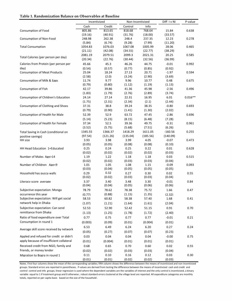
Diff I v NI P‐valueCash Credit Control Info
Consumption of Food 805.86 813.65 818.68 768.64 15.84 0.638(19.16) (40.91) (31.76) (18.00) (33.57)
Consumption of Non‐Food 248.98 262.38 248.4 237.35 12.23 0.278(5.84) (6.74) (9.28) (7.99) (11.20)
Total Consumption 1054.83 1076.03 1067.08 1005.99 28.06 0.465(21.11) (42.08) (34.55) (22.77) (38.29)2081.19 2079.51 2099.3 2021.31 20.25 0.585(20.34) (22.76) (30.44) (32.56) (36.99)45.66 45.3 46.26 44.75 ‐0.01 0.992(0.54) (0.57) (0.77) (0.85) (0.92)
Consumption of Meat Products 25.04 18.24 27.13 20.71 ‐1.97 0.594(2.58) (2.0) (3.24) (2.90) (3.69)
Consumption of Milk & Eggs 11.74 9.77 9.96 10.77 0.48 0.675(0.79) (0.80) (1.12) (1.19) (1.13)
Consumption of Fish 42.17 39.86 41.36 45.98 ‐2.56 0.496(1.83) (1.79) (2.76) (2.89) (3.74)
Consumption of Children's Education 24.14 27.14 22.31 16.95 6.01 0.016**(1.75) (2.31) (2.34) (2.1) (2.44)
Consumption of Clothing and Shoes 37.31 38.8 39.24 38.35 ‐0.80 0.693(0.79) (0.90) (1.41) (1.30) (2.02)
Consumption of Health for Male 52.39 52.9 63.72 47.45 ‐2.86 0.696(5.14) (5.23) (8.15) (6.48) (7.28)
Consumption of Health for Female 37.34 52.5 39.36 49.75 ‐0.31 0.961(3.52) (5.75) (5.68) (7.51) (6.26)1345.55 1366.37 1418.29 1611.05 ‐160.56 0.255(97.54) (121.26) (135.04) (185.56) (140.09)
HH size 3.93 3.98 3.99 4.05 ‐0.07 0.473(0.05) (0.05) (0.08) (0.08) (0.10)
HH Head Education 1=Educated 0.25 0.24 0.25 0.22 0.01 0.628(0.02) (0.02) (0.02) (0.02) (0.03)
Number of Males Age>14 1.19 1.22 1.18 1.18 0.03 0.515(0.02) (0.02) (0.03) (0.03) (0.04)
Number of Children Age<9 1.01 1.05 1.08 1.15 ‐0.09 0.093(0.03) (0.04) (0.05) (0.05) (0.05)
Household has pucca walls 0.29 0.32 0.27 0.30 0.02 0.55(0.02) (0.02) (0.03) (0.03) (0.04)
Literacy score average 3.37 3.40 3.48 3.30 ‐0.01 0.84(0.04) (0.04) (0.05) (0.06) (0.06)78.79 78.62 78.38 75.72 1.66 0.47(0.77) (0.88) (1.15) (1.35) (2.32)58.53 60.82 58.38 57.40 1.68 0.41(1.07) (1.21) (1.64) (1.61) (2.04)52.53 52.90 52.42 51.15 0.91 0.70(1.13) (1.25) (1.78) (1.72) (2.40)0.77 0.75 0.77 0.77 ‐0.01 0.21
(0.003) (0.09) (0.01) (0.004) (0.01)6.53 6.49 6.24 6.20 0.27 0.24(0.05) (0.27) (0.07) (0.07) (0.23)0.03 0.04 0.04 0.04 ‐0.00 0.75(0.01) (0.004) (0.01) (0.01) (0.01)0.68 0.65 0.70 0.60 0.02 0.55(0.02) (0.02) (0.03) (0.03) (0.04)
Migration to Bogra in round 1 0.11 0.10 0.16 0.12 0.03 0.30(0.01) (0.01) (0.02) (0.02) (0.03)
Table 1. Randomization Balance on Observables at BaselineIncentivized Non‐Incentivized
Notes. First four columns show the mean of the corresponding variables; fifth column shows the difference between the means of incentivized and non‐incentivized groups. Standard errors are reported in parentheses. P‐values are derived from testing the difference between the means of incentivized cash and credit and control control and info groups; linear regression is used where the dependent variables are the variables of interest and the only control is incentivized, a binary variable equal to 1 if treatment group and 0 otherwise ; robust standard errors clustered at the village level are reported. All expenditure categories are monthly totals, reported on per capita basis based on the size of the household .
Subjective expectation: Will get social network help in Dhaka
Ratio of food expenditure over Total Consumption in round 1
Average skill score received by network
Received credit from NGO, family and friends, or money lender
Calories from Protein (per person per day)
Subjective expectation: Monga occurrence this year
Subjective expectation: Can send remittance from Dhaka
Appled and refused for credit or didn't apply because of insufficient collateral
Total Calories (per person per day)
Total Saving in Cash (conditional on positive savings)

Migration Rate in 2008Cash 59.0%
(1.87)Credit 56.8%
(2.06)Info 35.9%
(2.80)Control 36.0%
(2.76)Incentivized Cash Credit Not Incentivized Diff (I‐NI)
58% 59.0% 56.8% 36% 22***(1.4) (1.87) (2.06) (1.96) (2.43)47% 45% 49% 37% 10***(1.41) (1.92) (2.12) (2.0) (2.46)44% 40% 50% 36% 8***(1.33) (3.04) (3.04) (1.51) (2.0)
Migration Rate in 2008
Migration Rate in 2009
Migration Rate in 2011
Table 2: Program Take‐up Rates
The P‐value is obtained from the testing difference between migration rates of incentivized (Cash and Credit) and non‐incentivized households (Info and Control), regardless of whether they accepted our cash or credit. No incentives were offered in 2009. For re‐migration rate in 2011, we compare migration rates in "pure control" villages that never received any incentives to villages that only received incentives in 2008 and never again.

Dependent Variable
Cash Credit Info
61.876** 50.044* 15.644 48.642** 44.183* 280.792** 260.139** 102.714***(29.048) (28.099) (40.177) (24.139) (23.926) (131.954) (128.053) (17.147)34.885*** 27.817** 22.843 20.367** 16.726* 115.003** 99.924* 59.085***(13.111) (12.425) (17.551) (9.662) (9.098) (56.692) (51.688) (8.960)96.566*** 76.743** 38.521 68.359** 60.139** 391.193** 355.115** 160.696***(34.610) (33.646) (50.975) (30.593) (29.683) (169.431) (158.835) (22.061)106.819* 93.429 ‐85.977 142.629*** 129.901*** 842.673*** 757.602*** 317.495***(62.974) (59.597) (76.337) (47.196) (48.057) (248.510) (250.317) (41.110)2.852* 2.588 ‐0.509 2.977** 2.657** 17.442** 15.573** 6.777***(1.557) (1.571) (2.089) (1.287) (1.273) (7.064) (6.830) (0.992)12.325** 6.577 8.163 5.618 5.599 31.857 34.302 3.905(5.489) (5.402) (6.667) (3.755) (3.726) (21.549) (21.399) (3.923)8.979* 12.618** 8.977 6.297 5.193 34.652 28.775 8.901**(4.743) (5.998) (6.076) (4.407) (4.142) (24.941) (22.909) (3.778)6.146* 7.658** 1.546 6.110** 4.299* 30.848** 21.487 ‐3.677(3.297) (3.441) (3.938) (2.485) (2.405) (14.144) (13.536) (2.355)
Sub‐district Fixed Effects? yes yes yes yes yes yes yes yesAdditional controls no no no no yes no yes no
Table 3: Effects of Migration before December 2008 on Consumption in 2008 Amongst Remaining Household Members
Robust standard errors in parentheses, clustered by village. *** p<0.01, ** p<0.05, * p<0.1. Each row is a different dependent variable (in column 1). In the IV columns, these dependent variables are regressed on "Migration", which is a binary variable equal to 1 if at least one member of the household migrated and 0 otherwise. The last column reports sample mean of the dependent variable in the control group. All consumption (expenditure) variables are measured in units of Takas per person per month, except Caloric Intake which is measured in terms of calories per person per day. Some expenditure items in the survey were asked over a weekly recall and other less frequently purchased items were asked over a bi‐weekly or monthly recall. The denominator of the dependent variable (household size) is the number of individuals who have been present in the house for at least seven days. Additional controls included in columns 5 and 7 were: household education, proxy for income (wall material), percentage of total expenditure on food, number of adult males, number of children, lacked access to credit, borrowing, total household expenditures per capita measured at baseline, and subjective expectations about Monga and social network support measured at baseline.
Consumption of Fish 67.3
Consumption of Children's Education
14.5
Total Calories (per person per day)
1976.1
Calories from Protein (per person per day) 44.0
Consumption of Meat Products 24.2
Consumption of Food 689.9
Consumption of Non‐Food 260.9
Total Consumption 950.8
MeanITT
OLSITT ITT IV IV
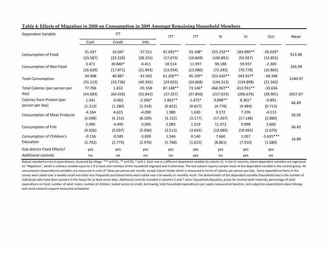
Dependent Variable
Cash Credit Info
31.437 16.047 ‐37.521 42.691** 33.108* 225.232** 183.990** ‐26.029*(23.587) (23.226) (28.255) (17.073) (16.849) (100.891) (92.927) (14.855)3.471 30.840* ‐4.411 18.514 11.997 98.188 59.937 ‐2.369
(16.629) (17.871) (21.943) (13.034) (13.080) (72.243) (70.778) (10.865)34.908 46.887 ‐41.932 61.205** 45.105* 323.420** 243.927* ‐28.398(31.113) (33.736) (40.345) (24.655) (24.668) (144.313) (134.898) (21.342)77.706 1.832 ‐91.558 87.148** 73.146* 466.907** 412.931** ‐33.656(54.683) (60.426) (55.842) (37.337) (37.850) (217.023) (206.676) (28.901)1.341 ‐0.062 ‐2.396* 1.862** 1.472* 9.898** 8.301* ‐0.891(1.213) (1.280) (1.314) (0.822) (0.827) (4.778) (4.484) (0.713)‐4.164 4.615 ‐4.090 1.980 1.630 9.572 7.376 ‐4.513(5.048) (5.151) (6.109) (3.152) (3.177) (17.267) (17.148) (2.880)5.090 ‐4.495 ‐3.045 2.083 1.519 11.072 9.998 2.600(4.926) (5.037) (5.936) (3.513) (3.642) (19.095) (19.492) (2.670)‐0.156 ‐0.585 ‐3.828 1.546 0.140 7.660 1.057 ‐5.635***(2.742) (2.774) (2.976) (1.768) (1.615) (8.861) (7.910) (1.680)
Sub‐district Fixed Effects? yes yes yes yes yes yes yes yesAdditional controls no no no no yes no yes noRobust standard errors in parentheses, clustered by village. *** p<0.01, ** p<0.05, * p<0.1. Each row is a different dependent variable (in column 1). In the IV columns, these dependent variables are regressed on "Migration", which is a binary variable equal to 1 if at least one member of the household migrated and 0 otherwise. The last column reports sample mean of the dependent variable in the control group. All consumption (expenditure) variables are measured in units of Takas per person per month, except Caloric Intake which is measured in terms of calories per person per day. Some expenditure items in the survey were asked over a weekly recall and other less frequently purchased items were asked over a bi‐weekly or monthly recall. The denominator of the dependent variable (household size) is the number of individuals who have been present in the house for at least seven days. Additional controls included in columns 5 and 7 were: household education, proxy for income (wall material), percentage of total expenditure on food, number of adult males, number of children, lacked access to credit, borrowing, total household expenditures per capita measured at baseline, and subjective expectations about Monga and social network support measured at baseline.
Consumption of Fish 66.45
Consumption of Children's Education
16.89
Total Calories (per person per day) 2057.67Calories from Protein (per person per day) 46.49
Consumption of Meat Products 26.56
Consumption of Food 913.98
Consumption of Non‐Food 326.99
Total Consumption 1240.97
Table 4: Effects of Migration in 2008 on Consumption in 2009 Amongst Remaining Household MembersITT
ITT ITT IV IV OLS Mean

All Migrants Incentivized Not Incentivized Diff Obs
Total Savings by household 3,490.47 3,506.59 3,434.94 71.65 951(97.22) (110.83) (202.80) (232.91)
Total Earnings by household 7,777.19 7,451.27 8,894.40 ‐1443.129** 952(244.77) (264.99) (586.14) (583.83)
Savings per day 56.76 56.46 57.79 ‐1.33 905(1.15) (1.29) (2.56) (2.77)
Earnings per day 99.39 96.09 111.15 ‐15.06** 926(1.75) (1.92) (4.0) (4.2)
Remittances per day 18.34 16.94 23.33 ‐6.39** 927(1.06) (1.19) (2.28) (2.55)
Travel Cost per Episode 264.55 264.12 266.00 ‐1.88 953(3.41) (3.80) (7.62) (8.16)
Table 5. Migrant Earnings and Savings at Destination (Data for Migrants Only; Non‐
*** p<0.01, ** p<0.05, * p<0.1. The "Diff" columns tests statistical differences between incentivized and non incentivized groups. Standard errors are reported in parentheses. The measures for total savings and earnings, and savings and earnings per day do not include outliers (Less than 20,000 for total savings and 120000 for earnings, individuals savings per day less than 500 and individuals ernings per day less than 700). Travel cost refers to the cost of food and travel to get to the destination. Average migration duration 76 days.

Sector Dhaka Mushigonj Tangail Bogra OtherTotal
earningsAgriculture 17.54 75.00 91.15 89.62 46.83 3230.52
(1.71) (2.50) (1.89) (2.26) (2.26) (77.68)Non‐ag day laborer 20.56 9.00 5.75 3.83 19.02 6039.72
(1.82) (1.66) (1.55) (1.42) (1.78) (317.52)Transport 40.93 11.00 1.33 1.09 15.34 4993.81
(2.21) (1.81) (0.76) (0.77) (1.63) (203.12)Other 20.97 5.00 1.77 5.46 18.81 5645.98
(1.83) (1.26) (0.88) (1.68) (1.77) (321.72)
Number of migration episodes 496 300 226 183 489 1,694
5005.06 3777.30 2897.88 2491.07 5160.60(185.92) (156.0) (145.72) (123.19) (188.69)
Table 6: 2008 Migrant Characteristics by Destination and by Sector
Notes: Standard errors are in parentheses. Shows the proportion of workers in each occupation by destination, average total earnings by sector across destinations, and average total earnings by destination across sectors. Based on migration for work episodes between September 1, 2008 to April 13, 2009. Occupation at the destination is based on the question, "In which sector were you employed (agriculture, industry, etc)?" Bogra and Tangail, which employ most migrant workers in the agriculture sector, are potato‐growing areas which do not follow the same crop and seasonal cycle as rice‐growing Rangpur.
Total earnings at Destination
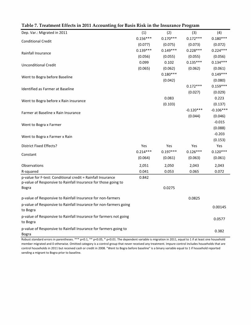
Dep. Var.: Migrated in 2011 (1) (2) (3) (4)0.156*** 0.170*** 0.172*** 0.180***(0.077) (0.075) (0.073) (0.072)0.139*** 0.149*** 0.228*** 0.224***(0.056) (0.055) (0.055) (0.056)0.099 0.102 0.135*** 0.134***(0.065) (0.062) (0.062) (0.061)
0.180*** 0.149***(0.042) (0.080)
0.172*** 0.159***(0.027) (0.029)
0.083 0.223(0.103) (0.137)
‐0.120*** ‐0.106***(0.044) (0.046)
‐0.015(0.088)‐0.203(0.153)
District Fixed Effects? Yes Yes Yes Yes0.214*** 0.197*** 0.126*** 0.120***(0.064) (0.061) (0.063) (0.061)
Observations 2,051 2,050 2,043 2,043R‐squared 0.041 0.053 0.065 0.072p‐value for F‐test: Conditional credit = Rainfall Insurance 0.842p‐value of Responsive to Rainfall Insurance for those going to Bogra 0.0275
p‐value of Responsive to Rainfall Insurance for non‐farmers 0.0825p‐value of Responsive to Rainfall Insurance for non‐farmers going to Bogra
0.00145
p‐value of Responsive to Rainfall Insurance for farmers not going to Bogra
0.0577
p‐value of Responsive to Rainfall Insurance for farmers going to Bogra
0.382
Table 7. Treatment Effects in 2011 Accounting for Basis Risk in the Insurance Program
Robust standard errors in parentheses. *** p<0.1, ** p<0.05, * p<0.01. The dependent variable is migration in 2011, equal to 1 if at least one household member migrated and 0 otherwise. Omitted category is a control group that never received any treatment. Impure control includes households that are control households in 2011 but received cash or credit in 2008. "Went to Bogra before baseline" is a binary variable equal to 1 if household reported sending a migrant to Bogra prior to baseline.
Constant
Farmer at Baseline x Rain Insurance
Identified as Farmer at Baseline
Went to Bogra before x Rain insurance
Went to Bogra x Farmer
Went to Bogra before Baseline
Went to Bogra x Farmer x Rain
Conditional Credit
Rainfall Insurance
Unconditional Credit

Dep. Var.: Migration in 2009 OLS IV OLS IV OLS IV OLS IV
0.392*** 0.410*** 0.392*** 0.464*** 0.393*** 0.436*** 0.392*** 0.476***(0.02) (0.145) (0.02) (0.133) (0.021) (0.132) (0.02) (0.13)
0.007 ‐0.006(0.01) (0.022)
‐0.012 ‐0.048(0.025) (0.049)
0.01 0.007(0.011) (0.027)
0.097*** 0.088 0.095** 0.062 0.098*** 0.078 0.095** 0.052(0.037) (0.083) (0.038) (0.078) (0.037) (0.076) (0.038) (0.077)
Observations 1818 1818 1818 1818 1797 1797 1797 1797R‐squared 0.207 0.206 0.207 0.201 0.208 0.206 0.209 0.202
Table 8. Learning from Own Experience and Othersʹ Experiences in 2009 Re‐migration Decision
*** p<0.01, ** p<0.05, * p<0.1 Robust standard errors in parentheses.
Did any member of the household migrate in 2008?
Number of friends and relatives who migrated
Number of friends who migrated
Number of relatives who migrated
Constant
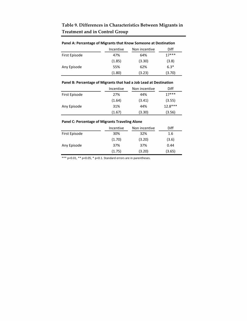
Incentive Non incentive DiffFirst Episode 47% 64% 17***
(1.85) (3.30) (3.8)Any Episode 55% 62% 6.3*
(1.80) (3.23) (3.70)
Incentive Non incentive DiffFirst Episode 27% 44% 17***
(1.64) (3.41) (3.55)Any Episode 31% 44% 12.8***
(1.67) (3.30) (3.56)
Incentive Non incentive DiffFirst Episode 30% 32% 1.6
(1.70) (3.20) (3.6)Any Episode 37% 37% 0.44
(1.75) (3.20) (3.65)
Table 9. Differences in Characteristics Between Migrants in Treatment and in Control Group
Panel A: Percentage of Migrants that Know Someone at Destination
Panel B: Percentage of Migrants that had a Job Lead at Destination
Panel C: Percentage of Migrants Traveling Alone
*** p<0.01, ** p<0.05, * p<0.1. Standard errors are in parentheses.
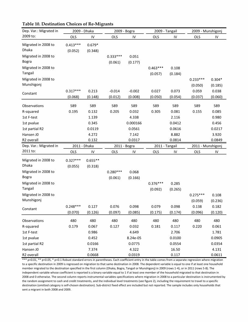
Table 10. Destination Choices of Re‐Migrants
OLS IV OLS IV OLS IV OLS IV
0.413*** 0.679*(0.052) (0.348)
0.333*** 0.051(0.061) (0.177)
0.463*** 0.108(0.057) (0.184)
0.233*** 0.304*(0.050) (0.185)
0.317*** 0.213 ‐0.014 ‐0.002 0.027 0.073 0.059 0.038(0.068) (0.148) (0.012) (0.008) (0.050) (0.054) (0.037) (0.060)
Observations 589 589 589 589 589 589 589 589R‐squared 0.195 0.132 0.205 0.032 0.305 0.081 0.155 0.0851st F‐test 1.139 4.338 2.116 0.9801st pvalue 0.345 0.000166 0.0412 0.4561st partial R2 0.0119 0.0561 0.0616 0.0217Hansen J0 4.272 7.142 8.882 3.920R2 overall 0.132 0.0317 0.0814 0.0849
OLS IV OLS IV OLS IV OLS IV
0.327*** 0.655**(0.055) (0.318)
0.280*** 0.068(0.061) (0.166)
0.376*** 0.285(0.092) (0.265)
0.275*** 0.108(0.059) (0.236)
0.248*** 0.127 0.076 0.098 0.079 0.098 0.138 0.182(0.070) (0.126) (0.097) (0.085) (0.175) (0.174) (0.096) (0.120)
Observations 480 480 480 480 480 480 480 480R‐squared 0.179 0.067 0.127 0.032 0.181 0.117 0.220 0.0611st F‐test 0.986 4.649 2.706 1.7811st pvalue 0.452 8.24e‐05 0.0100 0.09051st partial R2 0.0166 0.0775 0.0554 0.0354Hansen J0 7.374 4.322 16.50 4.131R2 overall 0.0668 0.0319 0.117 0.0611
Dep. Var.: Migrated in 2011 to:
Migrated in 2008 to Munshigonj
Constant
*** p<0.01, ** p<0.05, * p<0.1 Robust standard errors in parentheses. Each coefficient entry in the table comes from a separate regression where migration to a specific destination in 2009 is regressed on migration to that same destination in 2008. The dependent variable is equal to one if at least one household member migrated to the destination specified in the first column (Dhaka, Bogra, Tangail or Munshigonj) in 2009 (rows 1‐4), or in 2011 (rows 5‐8). The independent variable whose coefficient is reported is a binary variable equal to 1 if at least one member of the household migrated to that destination in 2008 and 0 otherwise. The second column reports instrumental variables specifications where migration in 2008 to a particular destination is instrumented by the random assignment to cash and credit treatments, and the individual level treatments (see figure 2), including the requirement to travel to a specific destination (omitted category is self‐chosen destination). Sub‐district fixed effect are included but not reported. The sample includes only households that sent a migrant in both 2008 and 2009.
2011 ‐ Bogra 2011 ‐ Tangail 2011 ‐ Munshigonj
Migrated in 2008 to DhakaMigrated in 2008 to BograMigrated in 2008 to Tangail
2011 ‐ Dhaka
2009 ‐ Munshigonj
Migrated in 2008 to BograMigrated in 2008 to TangailMigrated in 2008 to Munshigonj
Constant
Migrated in 2008 to Dhaka
Dep. Var.: Migrated in 2009 to:
2009 ‐ Dhaka 2009 ‐ Bogra 2009 ‐ Tangail

Table 11. Parameters Used for Calibration
Parameter Calibration Notes
u(c) (𝑐 − 𝑠)1−𝜎
1 − 𝜎 HARA utility function.
s 250 Taka per hh member
per month
Enough for about 600 Calories
per hh member per month
𝜋𝐺 0.5 The portion of induced migrants
that remigrate
F 250 Taka per hh member
per month
600 Taka for bus fare, plus 6
days of foregone labor at 60
Taka per day. Spread over 4 hh
members
m 550 per household member
per month
Solution to:
𝜋𝐺 (𝑚 + 𝐼) = 350
where 350 is our LATE estimate
and I is the size of our incentive.
𝜇(𝑦) 𝑁(700,7) per household
member, per month
Designed to look like the
distribution of the bottom half of
the population
Time Period 6 months
We assume the choice to migrate
can be made after planting for
either of the agricultural
seasons.
𝛿 0.99
I (incentive
size)
200 Taka per household
member Assumes a households size of 4
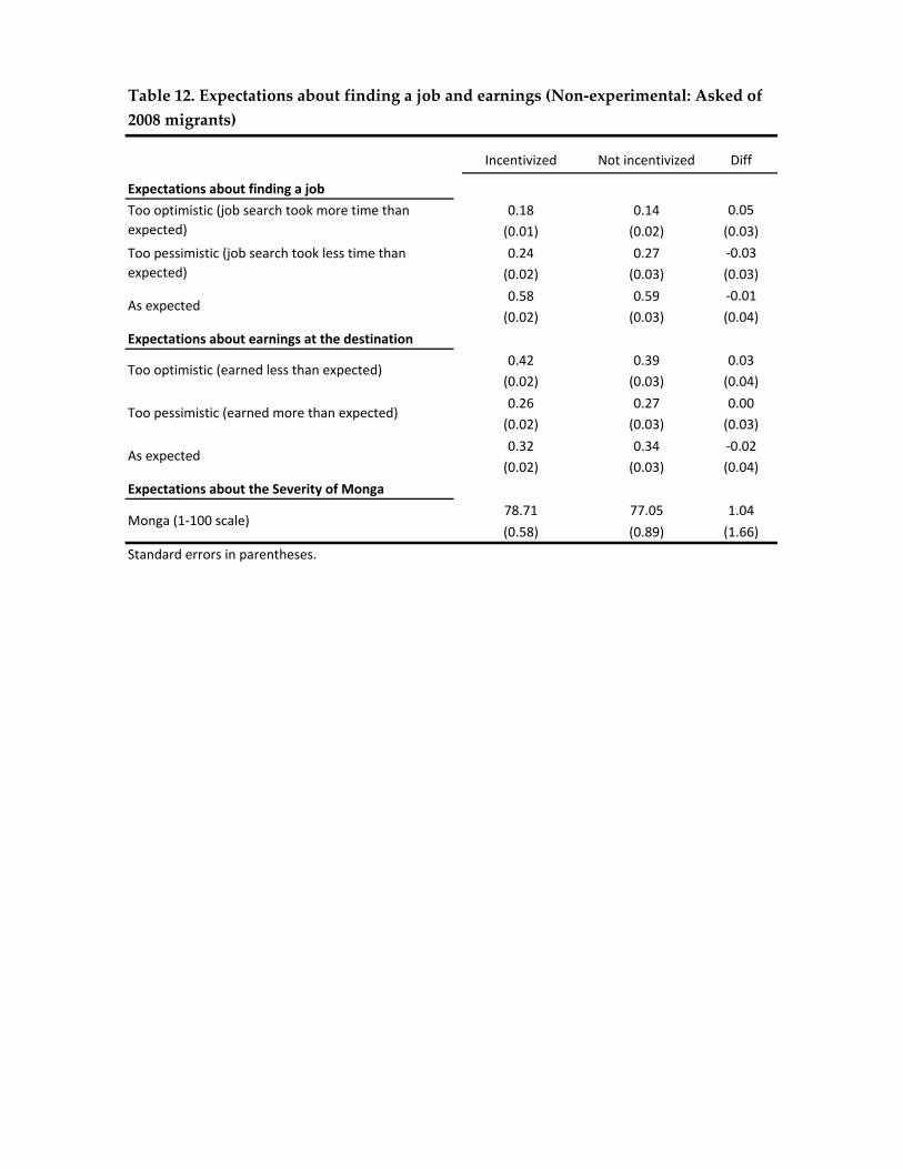
Incentivized Not incentivized Diff
Expectations about finding a job0.18 0.14 0.05(0.01) (0.02) (0.03)0.24 0.27 ‐0.03(0.02) (0.03) (0.03)0.58 0.59 ‐0.01(0.02) (0.03) (0.04)
Expectations about earnings at the destination0.42 0.39 0.03(0.02) (0.03) (0.04)0.26 0.27 0.00(0.02) (0.03) (0.03)0.32 0.34 ‐0.02(0.02) (0.03) (0.04)
Expectations about the Severity of Monga78.71 77.05 1.04(0.58) (0.89) (1.66)
Table 12. Expectations about finding a job and earnings (Non‐experimental: Asked of 2008 migrants)
Monga (1‐100 scale)
Standard errors in parentheses.
As expected
Too optimistic (job search took more time than expected)
Too pessimistic (job search took less time than expected)
As expected
Too optimistic (earned less than expected)
Too pessimistic (earned more than expected)

Figure 1. Seasonality in Consumption and Price in Rangpur and in Other Regions of Bangladesh
300
400
500
600
700
Taka
per
mon
th
1 2 3 4 5 6 7 8 9 10 11 12Months
Rest of the country Rangpur
HIES 2005Seasonality - Food Expenditure per capitaPanel B.
400
600
800
1000
Taka
per
mon
th
1 2 3 4 5 6 7 8 9 10 11 12Months
Rest of the country Rural Rangpur
HIES 2000Seasonality - Total Expenditures per CapitaPanel A.
.022
.024
HIES 2005Seasonality - Price of RicePanel C.
4550
old
HIES 2005Seasonality - Quantity Rice per HouseholdPanel D.
Source: Bangladesh Bureau of Statistics 2005 Household Income and Expenditure Survey
.016
.018
.02
Taka
per
Kg
1 2 3 4 5 6 7 8 9 10 11 12Months
Rest of the country Rangpur
3035
40K
g pe
r hou
seho
1 2 3 4 5 6 7 8 9 10 11 12Months
Rest of the country Rangpur
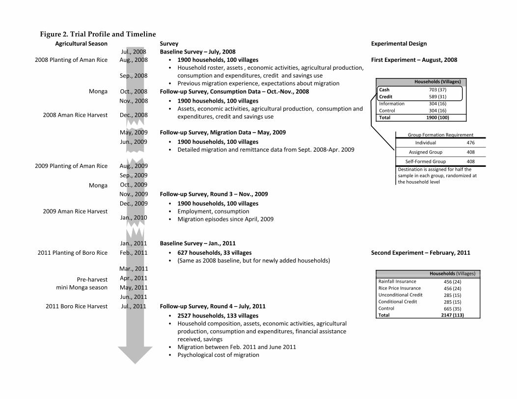
Agricultural Season Survey Experimental DesignJul., 2008 Baseline Survey – July, 2008
2008 Planting of Aman Rice Aug., 2008 • 1900 households, 100 villages• Household roster, assets , economic activities, agricultural production,
ti d dit dit d i
First Experiment – August, 2008
S 2008
Figure 2. Trial Profile and Timeline
consumption and expenditures, credit and savings use• Previous migration experience, expectations about migration
Monga
Sep., 2008
Oct., 2008 Follow‐up Survey, Consumption Data – Oct.‐Nov., 2008Nov., 2008 • 1900 households, 100 villages
• Assets, economic activities, agricultural production, consumption and expenditures, credit and savings use2008 Aman Rice Harvest Dec., 2008
Households (Villages)Cash 703 (37)Credit 589 (31)Information 304 (16)Control 304 (16)Total 1900 (100)
May, 2009 Follow‐up Survey, Migration Data – May, 2009Jun., 2009 • 1900 households, 100 villages
• Detailed migration and remittance data from Sept. 2008‐Apr. 2009
2009 Planting of Aman Rice Aug., 2009Sep 2009
Group Formation RequirementIndividual 476
Assigned Group 408
Self‐Formed Group 408Destination is assigned for half the
l i h d i d t
MongaSep., 2009Oct., 2009Nov., 2009 Follow‐up Survey, Round 3 – Nov., 2009
2009 Aman Rice HarvestDec., 2009 • 1900 households, 100 villages
• Employment, consumption• Migration episodes since April, 2009Jan., 2010
sample in each group, randomized at the household level
Jan., 2011 Baseline Survey – Jan., 20112011 Planting of Boro Rice Feb., 2011 • 627 households, 33 villages
• (Same as 2008 baseline, but for newly added households)Second Experiment – February, 2011
Mar., 2011Households (Villages)
Pre‐harvest mini Monga season
Apr., 2011May, 2011Jun., 2011
2011 Boro Rice Harvest Jul., 2011 Follow‐up Survey, Round 4 – July, 2011• 2527 households, 133 villages• Household composition, assets, economic activities, agricultural
Households (Villages)Rainfall Insurance 456 (24)Rice Price Insurance 456 (24)Unconditional Credit 285 (15)Conditional Credit 285 (15)Control 665 (35)Total 2147 (113)
Household composition, assets, economic activities, agricultural production, consumption and expenditures, financial assistance received, savings
• Migration between Feb. 2011 and June 2011• Psychological cost of migration
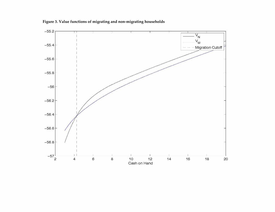
Figure 3. Value functions of migrating and non‐migrating households
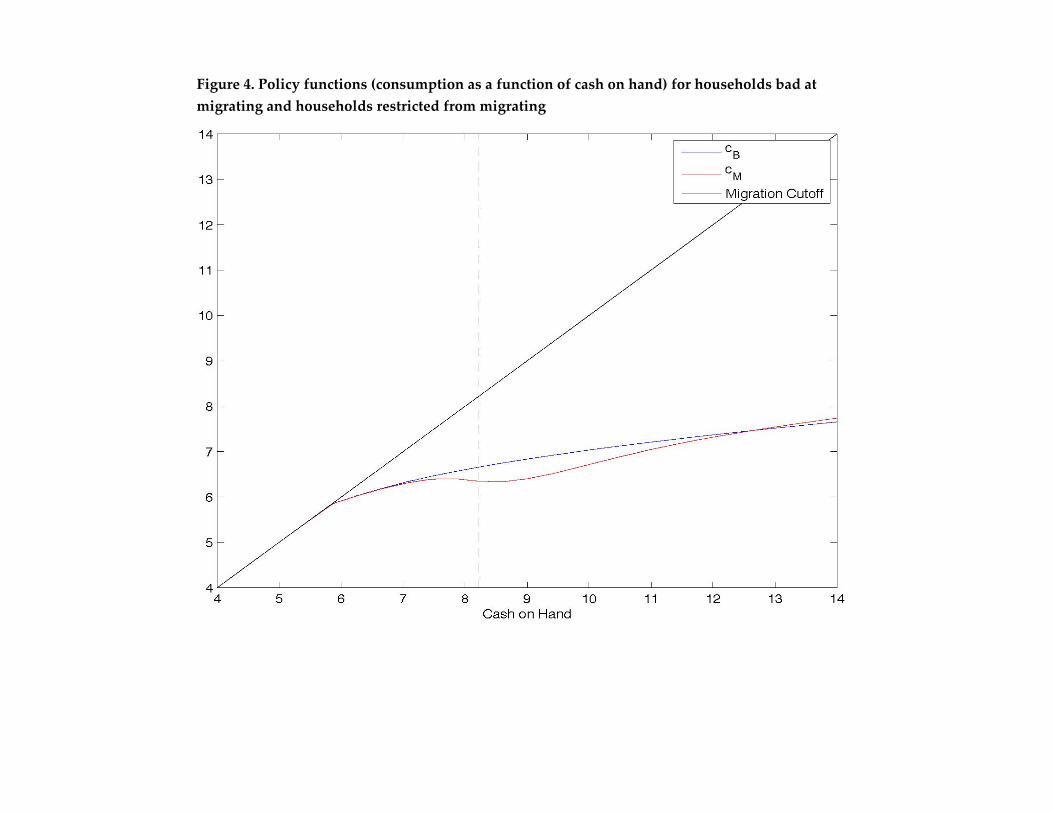
Figure 4. Policy functions (consumption as a function of cash on hand) for households bad at migrating and households restricted from migrating

Figure 5. Simulated Cahs on Hand and Consumptions for Varying Levels of WealthPanel A Panel B
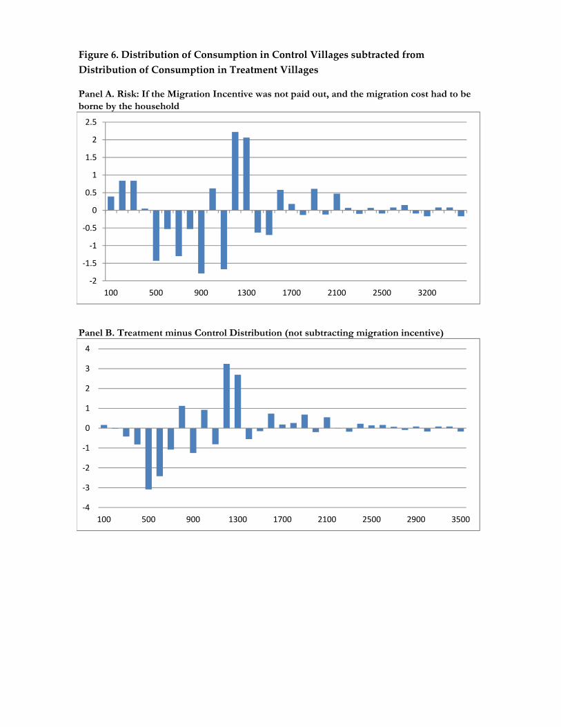
Figure 6. Distribution of Consumption in Control Villages subtracted from Distribution of Consumption in Treatment Villages
Panel A. Risk: If the Migration Incentive was not paid out, and the migration cost had to be borne by the household
Panel B. Treatment minus Control Distribution (not subtracting migration incentive)
‐2
‐1.5
‐1
‐0.5
0
0.5
1
1.5
2
2.5
100 500 900 1300 1700 2100 2500 3200
2
3
4
‐4
‐3
‐2
‐1
0
1
2
100 500 900 1300 1700 2100 2500 2900 3500
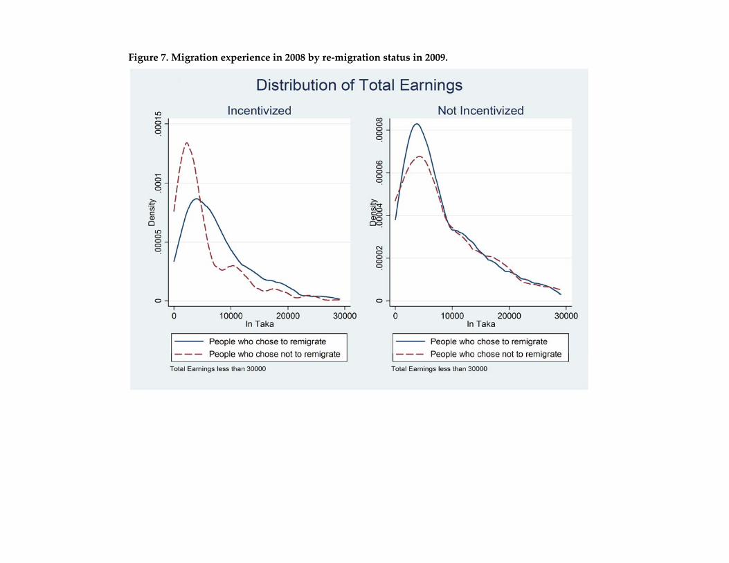
Figure 7. Migration experience in 2008 by re‐migration status in 2009.
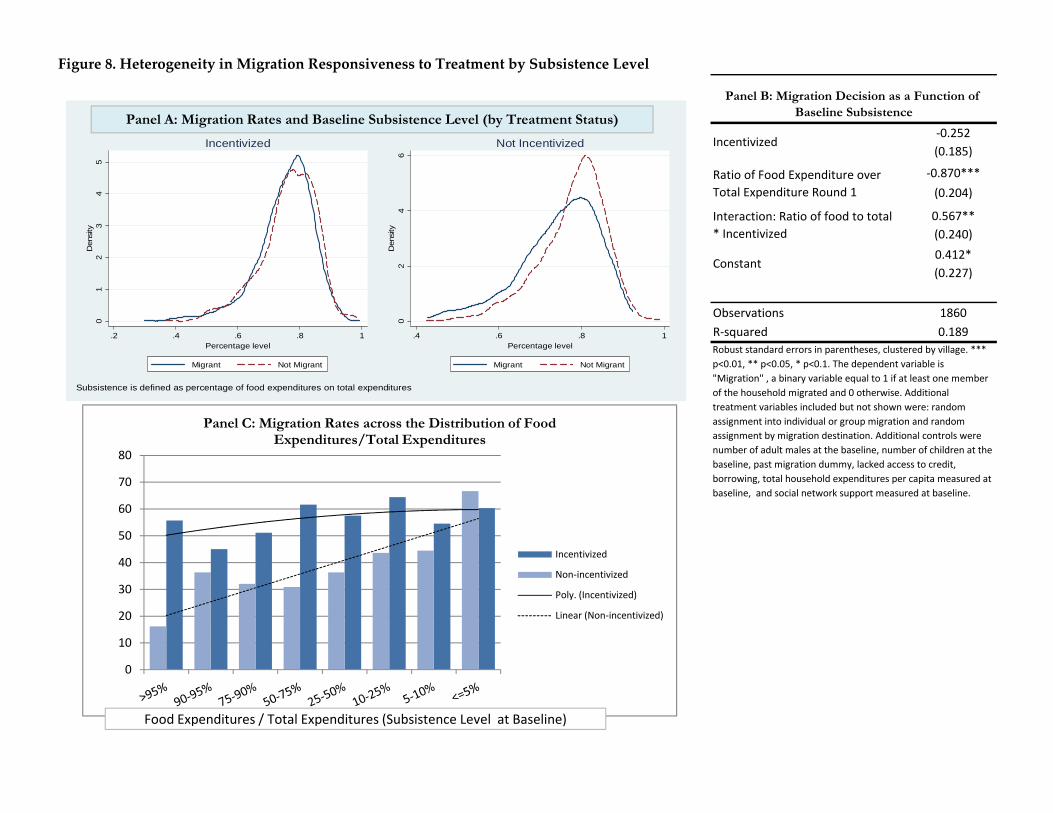
Figure 8. Heterogeneity in Migration Responsiveness to Treatment by Subsistence Level
‐0.252(0.185)
‐0.870***(0.204)
0.567**(0.240)0.412*(0.227)
Observations 1860R‐squared 0.189Robust standard errors in parentheses, clustered by village. *** p<0.01, ** p<0.05, * p<0.1. The dependent variable is "Migration" , a binary variable equal to 1 if at least one member of the household migrated and 0 otherwise. Additional treatment variables included but not shown were: random assignment into individual or group migration and random
b d dd l l
Panel B: Migration Decision as a Function of Baseline Subsistence
Incentivized
Ratio of Food Expenditure over Total Expenditure Round 1
Interaction: Ratio of food to total * Incentivized
Constant
01
23
45
Den
sity
.2 .4 .6 .8 1Percentage level
Migrant Not Migrant
Incentivized
02
46
Den
sity
.4 .6 .8 1Percentage level
Migrant Not Migrant
Not Incentivized
Subsistence is defined as percentage of food expenditures on total expenditures
Subsistence Level in Round 1 by Treatment
Panel C: Migration Rates across the Distribution of Food
Panel A: Migration Rates and Baseline Subsistence Level (by Treatment Status)
assignment by migration destination. Additional controls were number of adult males at the baseline, number of children at the baseline, past migration dummy, lacked access to credit, borrowing, total household expenditures per capita measured at baseline, and social network support measured at baseline.
0
10
20
30
40
50
60
70
80Expenditures/Total Expenditures
Incentivized
Non‐incentivized
Poly. (Incentivized)
Linear (Non‐incentivized)
Food Expenditures / Total Expenditures (Subsistence Level at Baseline)
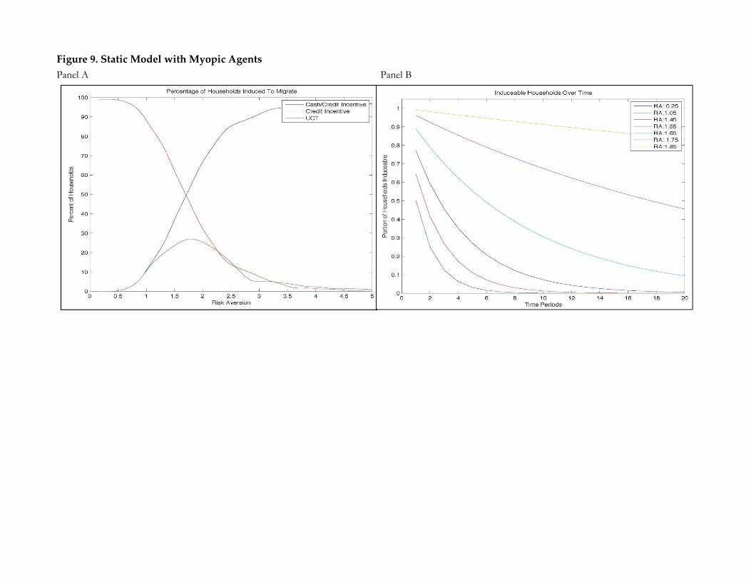
Figure 9. Static Model with Myopic AgentsPanel A Panel B
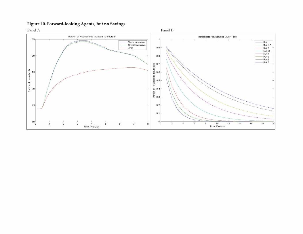
Figure 10. Forward‐looking Agents, but no SavingsPanel A Panel B
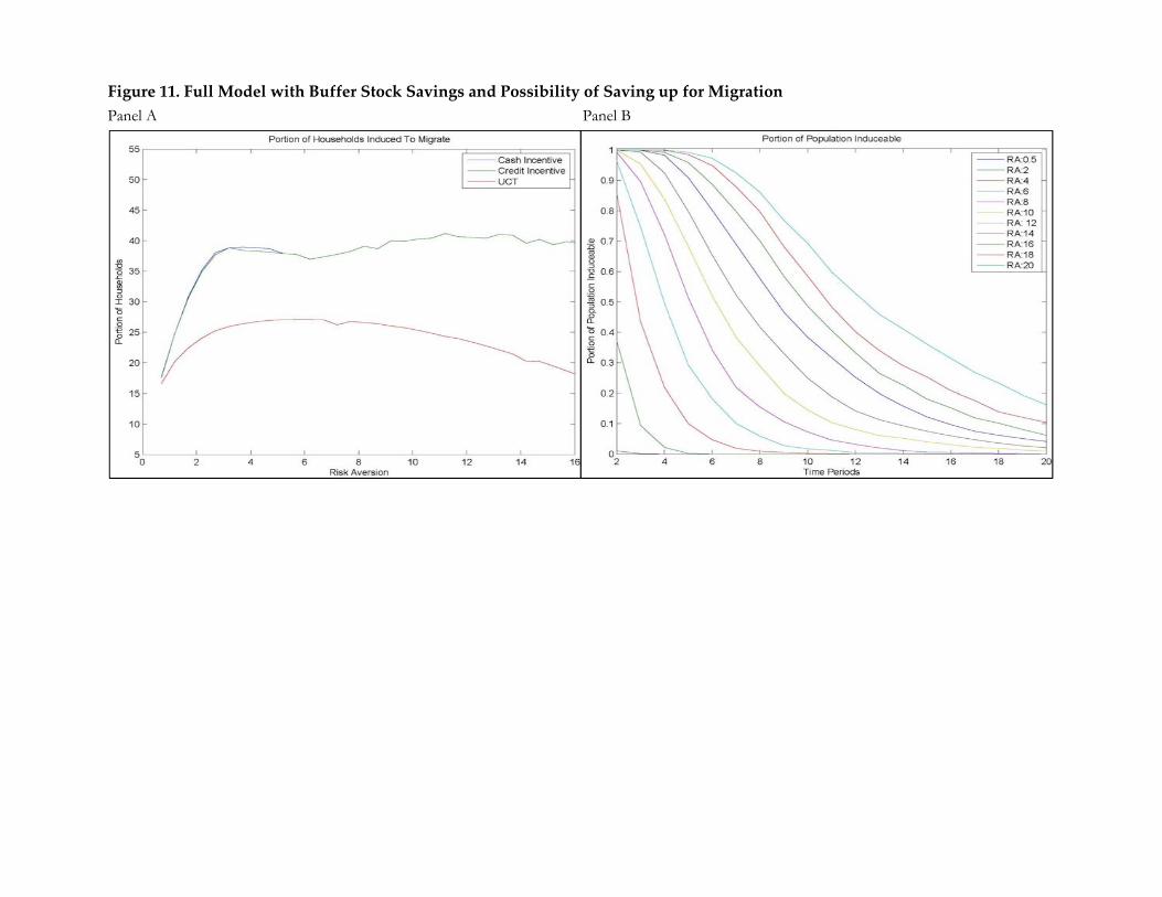
Figure 11. Full Model with Buffer Stock Savings and Possibility of Saving up for MigrationPanel A Panel B
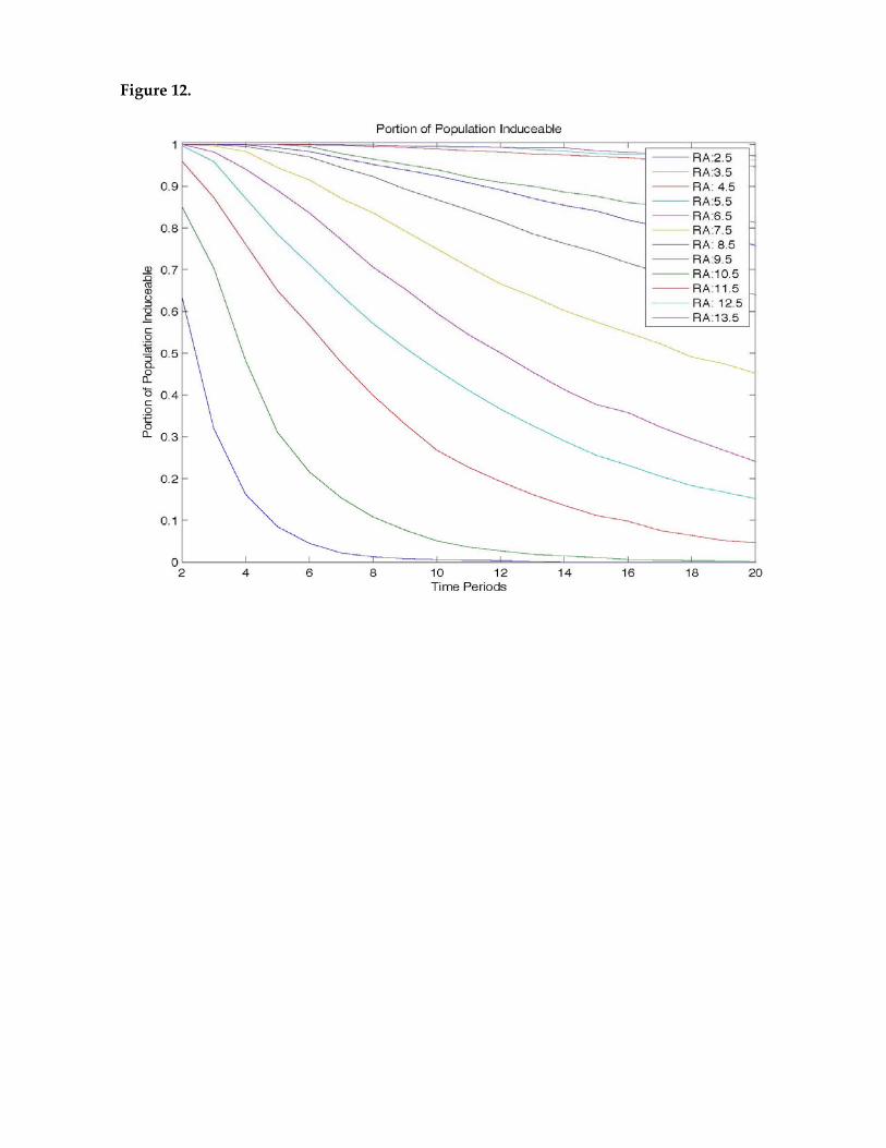
Figure 12.

1
Appendices for Bryan, Chowdhury and Mobarak (2013)
Appendix 1, 2, 3
Appendix Tables
Appendix Figures

2
Appendix 1 : Description of 2008 Treatments
Out of the 100 villages selected to participate in the study, 16 (304 households)
were assigned to the control group, while the remaining 84 villages (1596 households)
were assigned to one of three treatments:
Information (16 villages/304 households): Potential migrants were provided
with information on the types of jobs available in each of four areas: Bogra, Dhaka,
Munshigonj and Tangail. In addition, they were told the likelihood of finding such a
job, and the average daily wage in each job. This information was provided using the
following script:
“We would like to give you information on job availability, types of jobs available and
approximate wages in four regions – Bogra, Dhaka, Munshigonj and Tangail. They are not
in any particular order. NGOs working in those areas collected this information at the
beginning of this month.
Three most commonly available jobs in Bogra are: a) rickshaw pulling, b) construction
work, c) agricultural labor. The average wage rates per day are Tk. 150 to 200 for rickshaw
pulling, Tk.120 to 150 for construction work, and Tk. 80 to 100 for agricultural laborer. The
likelihood of getting such a job in Bogra is medium (not high/not low).
Three most commonly available jobs in Dhaka are: a) rickshaw pulling, b) construction
work, c) day labor. The average wage rates per day are Tk. 250 to 300 for rickshaw pulling,
Tk.200 to 250 for construction work, and Tk. 150 to 200 for day laborer. The likelihood of
getting such a job in Dhaka is high.
Three most commonly available jobs in Munshigonj are: a) rickshaw pulling, b) land
preparation for potato cultivation, c) agricultural laborer. The average wage rates per day
are Tk. 150 to 200 for rickshaw pulling, Tk.150 to 160 for land preparation, and Tk. 150 to
160 for agricultural laborer. The likelihood of getting such a job in Munshigonj is high.
Three most commonly available jobs in Tangail are: a) rickshaw pulling, b)
construction work, c) day laborer in brick fields. The average wage rates per day are Tk.
200 to 250 for rickshaw pulling, Tk.160 to 180 for construction work, and Tk. 150 to 200 for
brick field work. The likelihood of getting such a job in Tangail is medium (not high/not
low).
Based on the above information, would you/any member of your family like to any of
the above location during this monga season? If so, where do you want to go? Note that the
job market information given above might have changed or may change in the near future
and there is no guarantee that you will find a job, and we’re just providing you the best

3
information available to us. Note also that we or the NGOs that collected this information
will not provide you with any assistance in finding jobs in the destination.”
Cash (37 villages/703 households): Households were read the same script on job
availability as given above, and were also offered a cash grant of Taka 600 conditional
on migration. This money was provided at the origin prior to migration, and was
framed as defraying the travel cost (money for a bus ticket). Migrants had an
opportunity to receive Taka 200 more if they reported to us at the destination.
Credit (31 villages/589 households): Households were read the same script on
job availability as given above, and were also offered a zero interest loan of Taka 600
conditional on migration. This money was provided at the origin prior to migration,
and was framed as defraying the travel cost (money for a bus ticket). Migrants had an
opportunity to receive Taka 200 more if they reported to us at the destination.
Households were told that they would have to pay back the loan at the end of the
Monga season.

4
Appendix 2 : Description of Treatments in 2011
In 2011 we conducted one more round of randomized interventions in the same
sample of 1900 households (in 100 villages), plus 247 new households in 13 new
randomly selected villages from the same two districts (Kurigram and Lalmonirhat).
The treatments (most of which encouraged migration, like the 2008 experiments) were
randomized at the village level. They were offered in February, 2011, just before the
onset of the 2011 “mini‐Monga season,” which is the pre‐harvest lean season associated
with the lesser of the two annual rice harvests. The treatments were therefore designed
to encourage migration during this lean season. The same organization as in 2008 –
PKSF, and their local NGO partners – implemented the treatments. We collected follow
up data on all households in 133 villages in July‐August 2011.
Controls: All 16 Control villages from the 2008 experiments were retained as a
control group in 2011. We also chose not to intervene again in 19 villages that were
offered the credit treatment in 2008. These 19 villages are labeled “Impure Control” in
the regression table, and they allow us to study the long‐run effects of offering
migration credit in 2008.
Credit conditional on migration: Sample households in 15 villages received the
same zero‐interest loan conditional on a household member migrating, as offered in
2008. The credit amount was raised to Tk.800 (~US$10.8) to reflect inflation in the cost
of travel since 2008. Households were required to pay back in a single installment in
July, at the end of the lean season.
Unconditional credit: To test one of the implications of our model, we offered an
unconditional zero‐interest loan of Tk.800 to sample households in 15 villages. The loan
repayment terms were the same as the conditional credit, and no conditionality was
attached to the loan.
5
Conditional Credit with destination rainfall insurance: Sample households in
24 villages were offered the same zero interest Tk.800 (~US$10.8) credit conditional on
migration, but the repayment terms were conditioned on rainfall outcomes in one
popular migration destination: Bogra. Too much rainfall (and flooding) is a risk in
Bangladesh, and can lower migrant earnings, particularly for outdoor work like
rickshaw‐pulling and construction site work. We purchased 10 years of daily rainfall
data from the local meteorological department, imputed the probability distribution of
rainy days during the pre‐harvest migration period, and calculated the actuarially fair
insurance premium and payoff amounts. Our loan contract specified that if rainfall in
Bogra for March/April 2011 remained “normal” (4 days or less), the migrants would
have to pay back Tk. 950 (~US$12.83). For 5‐9 days of rainfall, the repayment
requirement would be Tk.714 (~US$9.64). For 10 or more days of rainfall, the repayment
requirement was Tk.640 (~US$8.64). The amounts were chosen to make the insurance
contract actuarially fair, given historical rainfall data.
Note that this is a loan contract, but the repayment rules introduce a feature of
index insurance against too much rainfall.1 The treatment design takes advantage of the
fact that the contract offers differential basis risk for households that differ along
identifiable baseline characteristics: those who had a propensity for traveling to Bogra,
and non‐farmers. Basis risk from the index contract is lower for these two groups.
All treatments described above were proportionally balanced across the
Information, Cash and Credit treatments from 2008 (and Control villages from 2008
were retained as long‐term controls as described above). In some other sample villages
from 2008, we conducted other treatments that are not relevant for the analysis
conducted in this paper, and we therefore do not discuss those treatments here.
1 Note that the contract can be explained to borrowers like a standard credit contract, and the insurance feature is only introduced
because the credit repayment is state contingent. This helps to avoid confusion about the concept of insurance (Gine and Yang 2009).
6
Appendix 3 : Risk Aversion, Insurance and Basis Risk
This appendix provides a simple model of basis risk based on Clarke (2011) and
uses it to argue that our 2011 insurance experiment can be used to test whether
migration is risky and migrants are risk averse.2
There are two payoff relevant states {L,H} which lead to income at the destination
. We assume . There are two rainfall states , and rainfall
insurance makes a payment of p in state and costs c in state . We denote
. This setup leads to four possible states of the world , , , . Following
Clarke we parameterize basis risk with a variable – that is, the probability
that income is low but that the insurance contract does not payout and is in fact costly.3
This implies that the remaining probabilities are
1 ; ;
We assume that r depends on the characteristics of the migrator. In particular, we
assume:
1. Basis risk is larger for farmers than for non‐farmers ; and
2. Basis risk is smaller for those that are more likely to migrate to Bogra: .
We make the first assumption because the insurance contract pays in a high rain
situation. High rain is likely to reduce income of day laborers who work, for example,
pulling rickshaws. For agricultural laborers, however, high rain is potential
advantageous as it is likely to increase work. We make the second assumption because
the rainfall data is collected in Bogra and will be less accurate in other destinations. This
leads to the possibility that we record high rainfall, but there is in fact low rainfall in, for
2 See also Bryan (2012) for an application of the model presented here. 3 Recall that our insurance project pays out in the high rainfall state.

7
example, Dhaka. We make no assumption about the relative basis risk for those that are
farmer going to Bogra versus non‐farmers that are not going to Bogra.
We are interested in deriving the relative impact of the provision of insurance on
the migration rate. To do so, we suppose that potential migrators all face the same
(expected) income given migration (i.e. there is no heterogeneity in the migration
process except for r), but that potential migrators are heterogeneous with respect to
their returns to remaining at home.4 In particular, we assume that the expected utility
of remaining at home is migrator specific and given by which we assume to be
distributed according to F.
Given these assumptions, the portion of potential migrators that migrate without
insurance is given by
1 ,
and with insurance by
1
If F does not depend on the type of migrator except, perhaps, through purely
horizontal shifts, then the change in the probability of migration (or equivalently the
portion of the population migrating) is proportional to
1
1 .
Given this setup, we say that migration is risky if . The model implies the
following:
4 This is easily generalized and our regressions presented in the main text allow for differences in the return to
migration for farmers, non-farmers and those that are going to Bogra.
8
Proposition 1 (Basis risk is only relevant if migration is risky). The portion of
people induced to migrate by insurance is decreasing in r if and only if migration is risky and
migrators are risk averse.
Proof. The “only if” follows because r drops out of (1) when migration is not
risky. The “if” follows because an increase in r is a mean preserving spread, so the left
hand side of (1) must be decreasing in r so long as migrators are risk averse.
This proposition, combined with our assumptions on r leads to the following
joint test:
Hypothesis 1 (Basis risk implies migration is risky). If migration is risky, then
rainfall insurance will increase migration rates more for those that are migrating to Bogra and
more for non‐farmers.
The nature of this hypothesis is that, if the model of basis risk is correct, and our
assumptions about the relative amounts of basis risk are correct, then we can infer that
migration itself is risky from the results of our insurance experiment.
References
Bryan, G. (2012). Ambiguity and insurance. Unpublished manuscript.
Clarke, D. J. (2011). A theory of rational demand for index insurance. (Department of
Economics Discussion Paper Series No. 572).University of Oxford. Retrieved from
http://www.economics.ox.ac.uk/index.php/department‐of‐economics‐discussion‐
paper‐series/a‐theory‐of‐rational‐demand‐for‐index‐insurance
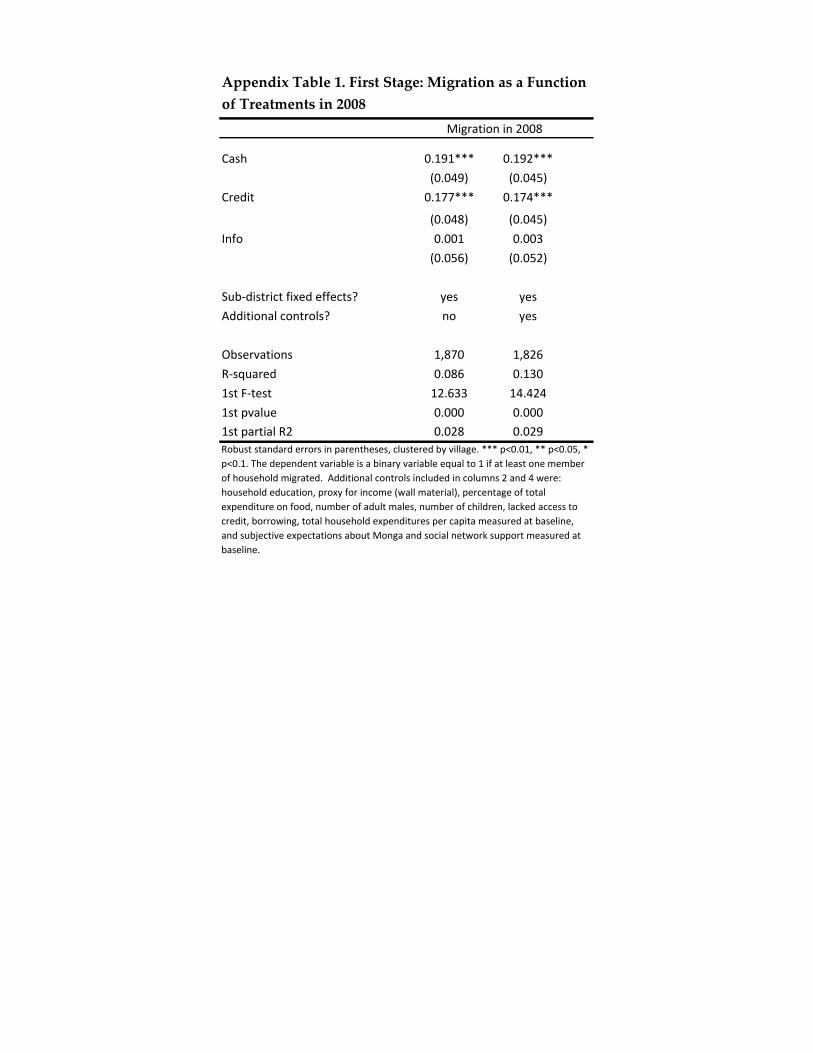
Cash 0.191*** 0.192***(0.049) (0.045)
Credit 0.177*** 0.174***
(0.048) (0.045)Info 0.001 0.003
(0.056) (0.052)
Sub‐district fixed effects? yes yesAdditional controls? no yes
Observations 1,870 1,826R‐squared 0.086 0.1301st F‐test 12.633 14.4241st pvalue 0.000 0.0001st partial R2 0.028 0.029
Migration in 2008
Robust standard errors in parentheses, clustered by village. *** p<0.01, ** p<0.05, * p<0.1. The dependent variable is a binary variable equal to 1 if at least one member of household migrated. Additional controls included in columns 2 and 4 were: household education, proxy for income (wall material), percentage of total expenditure on food, number of adult males, number of children, lacked access to credit, borrowing, total household expenditures per capita measured at baseline, and subjective expectations about Monga and social network support measured at baseline.
Appendix Table 1. First Stage: Migration as a Function of Treatments in 2008
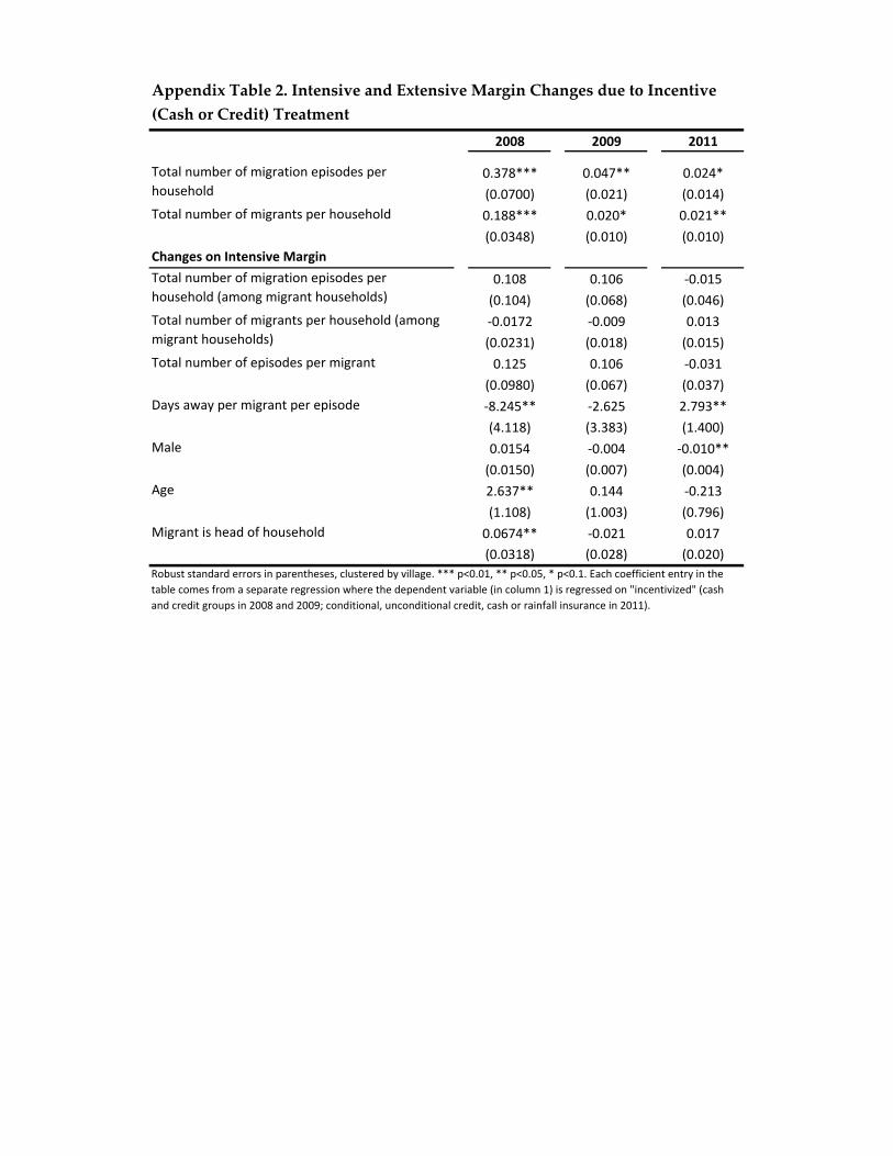
2008 2009 2011
0.378*** 0.047** 0.024*(0.0700) (0.021) (0.014)0.188*** 0.020* 0.021**(0.0348) (0.010) (0.010)
Changes on Intensive Margin0.108 0.106 ‐0.015(0.104) (0.068) (0.046)‐0.0172 ‐0.009 0.013(0.0231) (0.018) (0.015)0.125 0.106 ‐0.031
(0.0980) (0.067) (0.037)‐8.245** ‐2.625 2.793**(4.118) (3.383) (1.400)0.0154 ‐0.004 ‐0.010**(0.0150) (0.007) (0.004)2.637** 0.144 ‐0.213(1.108) (1.003) (0.796)0.0674** ‐0.021 0.017(0.0318) (0.028) (0.020)
Robust standard errors in parentheses, clustered by village. *** p<0.01, ** p<0.05, * p<0.1. Each coefficient entry in the table comes from a separate regression where the dependent variable (in column 1) is regressed on "incentivized" (cash and credit groups in 2008 and 2009; conditional, unconditional credit, cash or rainfall insurance in 2011).
Appendix Table 2. Intensive and Extensive Margin Changes due to Incentive (Cash or Credit) Treatment
Total number of migration episodes per household (among migrant households)
Total number of migrants per household (among migrant households)
Total number of episodes per migrant
Days away per migrant per episode
Male
Age
Migrant is head of household
Total number of migration episodes per household
Total number of migrants per household

Dependent VariableCash Credit Info
49.674** 48.292** 20.427 39.033* 222.288* ‐7.835(23.752) (23.015) (36.787) (21.745) (124.365) (15.422)35.320** 28.121** 20.817 21.721** 122.929* 32.930***(14.941) (14.046) (18.860) (10.348) (63.274) (8.621)
104.162*** 86.081*** 41.620 75.234** 429.585** 61.339***(32.672) (31.318) (49.635) (30.031) (176.462) (20.343)120.927** 111.339** ‐66.444 148.964*** 869.842*** 102.951***(54.673) (51.398) (68.194) (42.735) (243.784) (38.129)
50.506* 46.669* 5.063 46.219* 267.336** 67.936***(26.961) (26.185) (38.967) (23.648) (133.310) (17.226)29.778** 25.690* 18.536 18.774* 106.119* 45.519***(13.686) (13.495) (18.144) (9.917) (59.272) (9.152)80.085** 71.211** 23.634 64.328** 368.937** 112.357***(31.663) (31.784) (49.575) (29.958) (171.948) (22.179)69.645 77.571 ‐117.409 130.875*** 775.485*** 218.266***(65.251) (62.278) (76.655) (48.946) (274.635) (41.640)
56.019* 49.215* 21.065 42.498* 243.791* 80.573***(28.385) (27.493) (40.053) (24.070) (132.883) (16.898)32.313** 27.335** 25.281 17.586* 98.361* 49.524***(13.170) (12.594) (17.941) (9.593) (56.223) (8.738)88.138** 75.440** 46.380 59.440* 337.769** 129.019***(34.016) (33.216) (51.202) (30.518) (170.467) (21.769)90.556 91.954 ‐69.585 125.294*** 737.107*** 252.609***(60.478) (56.772) (75.689) (46.656) (249.228) (40.847)
Appendix Table 3. Effects of Migration in 2008 on Consumption in 2008; Sensitivity to Changes in Definition of Household Size
ITTITT IV OLS
Panel A: number of household members is based on question Q7 in R2 follow-up survey ("status of household members")
Panel B: number of household members is based on Q9 in R2 follow-up survey ("currently present members")
Panel C: household size is based on the total number of household members at the time of the interview
Total Calories (per person per day)
Consumption of Food
Consumption of Non‐Food
Consumption of Food
Consumption of Non‐Food
Total Consumption
Total Consumption
Consumption of Food
Consumption of Non‐Food
Total Consumption
Total Calories (per person per day)
Total Calories (per person per day)
Robust standard errors in parentheses, clustered by village. *** p<0.01, ** p<0.05, * p<0.1.
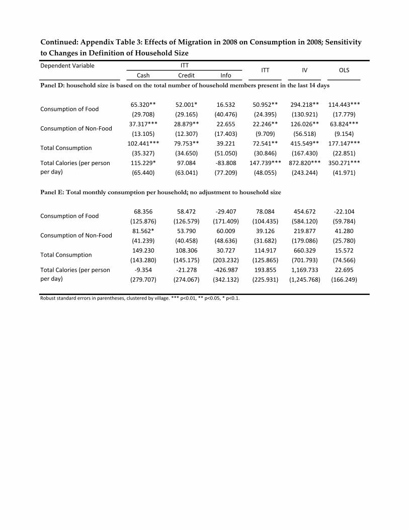
Dependent VariableCash Credit Info
65.320** 52.001* 16.532 50.952** 294.218** 114.443***(29.708) (29.165) (40.476) (24.395) (130.921) (17.779)37.317*** 28.879** 22.655 22.246** 126.026** 63.824***(13.105) (12.307) (17.403) (9.709) (56.518) (9.154)
102.441*** 79.753** 39.221 72.541** 415.549** 177.147***(35.327) (34.650) (51.050) (30.846) (167.430) (22.851)115.229* 97.084 ‐83.808 147.739*** 872.820*** 350.271***(65.440) (63.041) (77.209) (48.055) (243.244) (41.971)
68.356 58.472 ‐29.407 78.084 454.672 ‐22.104(125.876) (126.579) (171.409) (104.435) (584.120) (59.784)81.562* 53.790 60.009 39.126 219.877 41.280(41.239) (40.458) (48.636) (31.682) (179.086) (25.780)149.230 108.306 30.727 114.917 660.329 15.572(143.280) (145.175) (203.232) (125.865) (701.793) (74.566)‐9.354 ‐21.278 ‐426.987 193.855 1,169.733 22.695
(279.707) (274.067) (342.132) (225.931) (1,245.768) (166.249)
Consumption of Food
Consumption of Non‐Food
Robust standard errors in parentheses, clustered by village. *** p<0.01, ** p<0.05, * p<0.1.
Consumption of Food
Consumption of Non‐Food
Total Consumption
Total Calories (per person per day)
Total Calories (per person per day)
Continued: Appendix Table 3: Effects of Migration in 2008 on Consumption in 2008; Sensitivity to Changes in Definition of Household Size
ITT
Total Consumption
ITT IV OLS
Panel D: household size is based on the total number of household members present in the last 14 days
Panel E: Total monthly consumption per household; no adjustment to household size
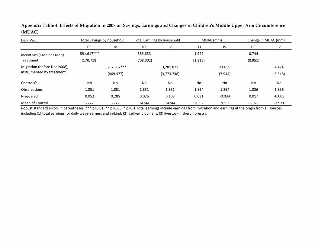
Dep. Var.:
ITT IV ITT IV ITT IV ITT IV
591.617*** 585.653 1.929 0.744
(170.718) (708.002) (1.315) (0.951)
3,287.602*** 3,281.877 11.059 4.474
(869.377) (3,773.748) (7.944) (5.348)
Controls? No No No No No No No No
Observations 1,851 1,851 1,851 1,851 1,854 1,854 1,836 1,836
R‐squared 0.052 0.285 0.026 0.103 0.031 ‐0.034 0.017 ‐0.005
Mean of Control 2272 2272 14244 14244 205.2 205.2 ‐3.971 ‐3.971
Appendix Table 4. Effects of Migration in 2008 on Savings, Earnings and Changes in Childrenʹs Middle Upper Arm Circumference (MUAC)
Migration (before Dec 2008), instrumented by treatment
Total Savings by household Total Earnings by household MUAC (mm) Change in MUAC (mm)
Robust standard errors in parentheses. *** p<0.01, ** p<0.05, * p<0.1 Total earnings include earnings from migration and earnings at the origin from all sources, including (1) total earnings for daily wage‐earners and in‐kind; (2) self‐employment; (3) livestock; fishery; forestry.
Incentives (Cash or Credit) Treatment
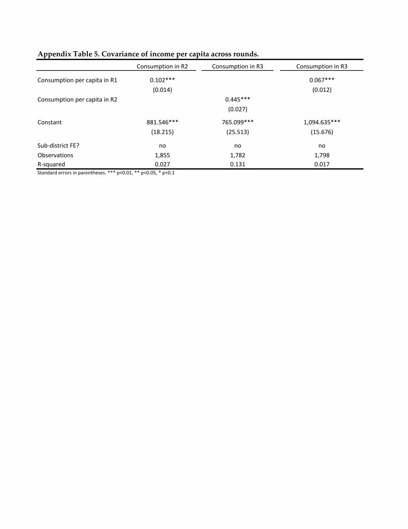
Consumption per capita in R1 0.102*** 0.067***(0.014) (0.012)
Consumption per capita in R2 0.445***(0.027)
Constant 881.546*** 765.099*** 1,094.635***(18.215) (25.513) (15.676)
Sub‐district FE? no no noObservations 1,855 1,782 1,798R‐squared 0.027 0.131 0.017Standard errors in parentheses. *** p<0.01, ** p<0.05, * p<0.1
Consumption in R2 Consumption in R3 Consumption in R3
Appendix Table 5. Covariance of income per capita across rounds.
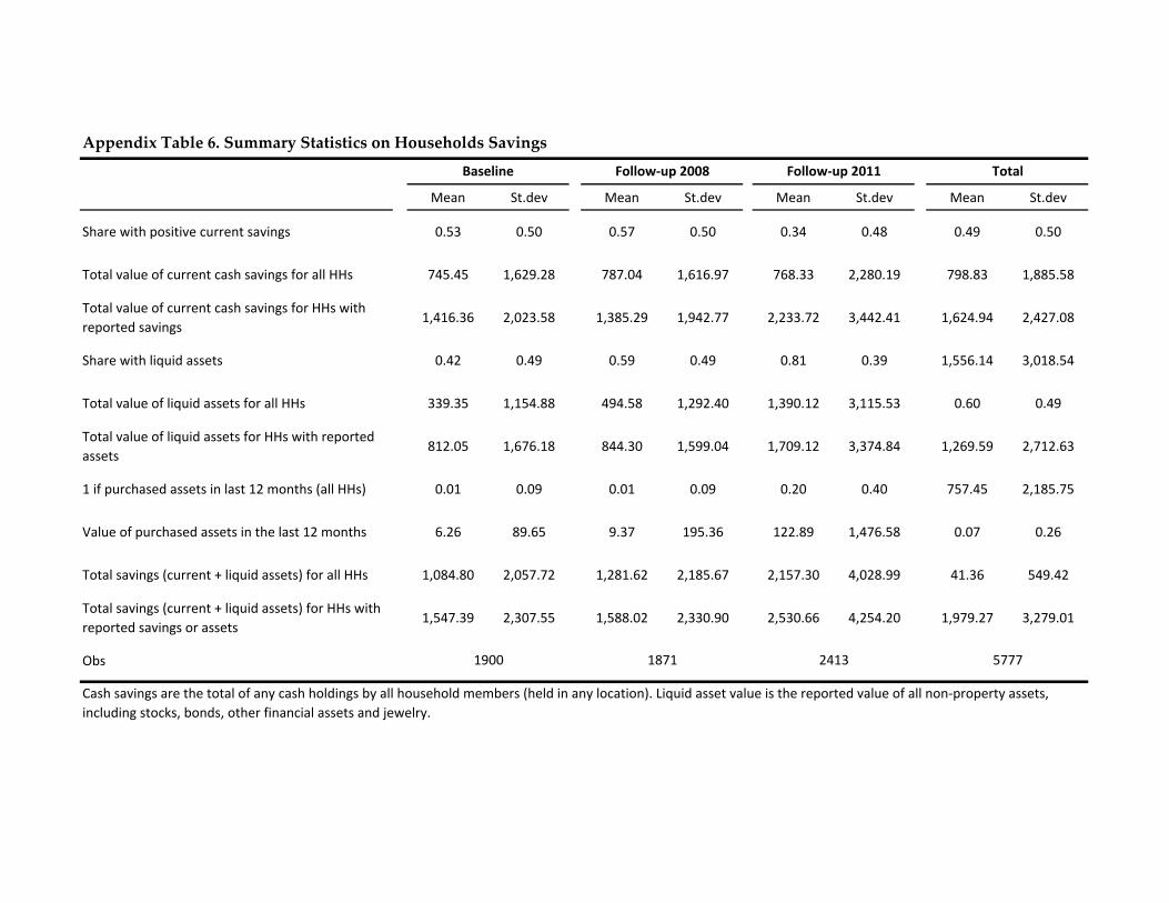
Mean St.dev Mean St.dev Mean St.dev Mean St.dev
Share with positive current savings 0.53 0.50 0.57 0.50 0.34 0.48 0.49 0.50
Total value of current cash savings for all HHs 745.45 1,629.28 787.04 1,616.97 768.33 2,280.19 798.83 1,885.58
Total value of current cash savings for HHs with reported savings
1,416.36 2,023.58 1,385.29 1,942.77 2,233.72 3,442.41 1,624.94 2,427.08
Share with liquid assets 0.42 0.49 0.59 0.49 0.81 0.39 1,556.14 3,018.54
Total value of liquid assets for all HHs 339.35 1,154.88 494.58 1,292.40 1,390.12 3,115.53 0.60 0.49
Total value of liquid assets for HHs with reported assets
812.05 1,676.18 844.30 1,599.04 1,709.12 3,374.84 1,269.59 2,712.63
1 if purchased assets in last 12 months (all HHs) 0.01 0.09 0.01 0.09 0.20 0.40 757.45 2,185.75
Value of purchased assets in the last 12 months 6.26 89.65 9.37 195.36 122.89 1,476.58 0.07 0.26
Total savings (current + liquid assets) for all HHs 1,084.80 2,057.72 1,281.62 2,185.67 2,157.30 4,028.99 41.36 549.42
Total savings (current + liquid assets) for HHs with reported savings or assets
1,547.39 2,307.55 1,588.02 2,330.90 2,530.66 4,254.20 1,979.27 3,279.01
Obs
Cash savings are the total of any cash holdings by all household members (held in any location). Liquid asset value is the reported value of all non‐property assets, including stocks, bonds, other financial assets and jewelry.
Follow‐up 2011 Total
Appendix Table 6. Summary Statistics on Households Savings
1900 1871 2413 5777
Baseline Follow‐up 2008

Full sample
Incentivized in 2008 0.047*(0.027)
Constant 0.266***(0.020)
Observations 2,771R‐squared 0.003
Appendix Table 7. Going Back to the Same Employer in 2011
Notes. Robust standard errors in parentheses. *** p<0.01, ** p<0.05, * p<0.1. The dependent variable in "Full sample" is equal to 1 if a respondent reports going to the same employer in 2011 as before; 0 otherwise. The dependent variable in "Migrant only" is equal to 1 if a respondent reports going to the same employer in 2011 as before; it is equal to 0 if a migrant reports going to a different employer as before (of migrants who travelled to the same place as before).
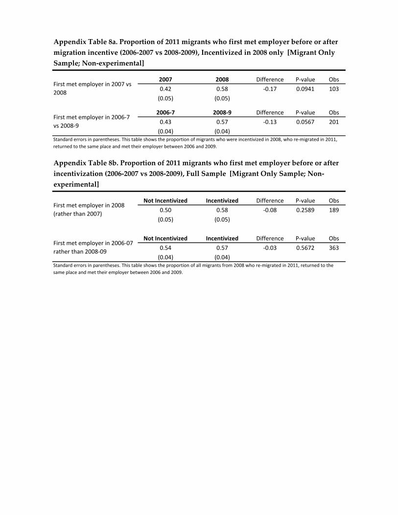
2007 2008 Difference P‐value Obs0.42 0.58 ‐0.17 0.0941 103(0.05) (0.05)
2006‐7 2008‐9 Difference P‐value Obs0.43 0.57 ‐0.13 0.0567 201(0.04) (0.04)
Not Incentivized Incentivized Difference P‐value Obs0.50 0.58 ‐0.08 0.2589 189(0.05) (0.05)
Not Incentivized Incentivized Difference P‐value Obs0.54 0.57 ‐0.03 0.5672 363(0.04) (0.04)
Standard errors in parentheses. This table shows the proportion of all migrants from 2008 who re‐migrated in 2011, returned to the same place and met their employer between 2006 and 2009.
First met employer in 2006‐7 vs 2008‐9
First met employer in 2007 vs 2008
Appendix Table 8a. Proportion of 2011 migrants who first met employer before or after migration incentive (2006‐2007 vs 2008‐2009), Incentivized in 2008 only [Migrant Only Sample; Non‐experimental]
Standard errors in parentheses. This table shows the proportion of migrants who were incentivized in 2008, who re‐migrated in 2011, returned to the same place and met their employer between 2006 and 2009.
Appendix Table 8b. Proportion of 2011 migrants who first met employer before or after incentivization (2006‐2007 vs 2008‐2009), Full Sample [Migrant Only Sample; Non‐experimental]
First met employer in 2008 (rather than 2007)
First met employer in 2006‐07 rather than 2008‐09

Dep. Var.: Migrated in 2008 to: Dhaka Bogra Tangail Munshigonj
‐0.032 0.125** ‐0.052 0.010(0.088) (0.051) (0.075) (0.083)0.035 0.085* 0.017 ‐0.056(0.088) (0.048) (0.077) (0.083)0.009 0.052 0.016 0.019(0.102) (0.049) (0.088) (0.094)‐0.045 0.022 ‐0.022 ‐0.011(0.046) (0.053) (0.054) (0.051)‐0.001 0.053 ‐0.041 0.008(0.058) (0.057) (0.051) (0.049)‐0.048 ‐0.018 0.059 0.054(0.050) (0.052) (0.066) (0.072)‐0.020 ‐0.059* ‐0.078* ‐0.007(0.044) (0.033) (0.045) (0.037)0.054(0.068)
0.234***(0.066)
0.305***(0.084)
0.163**(0.080)
0.427*** ‐0.075* 0.142* 0.295(0.148) (0.043) (0.072) (0.187)
Observations 589 589 589 589R‐squared 0.092 0.103 0.197 0.097
Appendix Table 9. First stage of Instrumental Variables Regression for Destination Choices
*** p<0.01, ** p<0.05, * p<0.1. Robust standard errors in parentheses.
Constant
Cash
Credit
Info
Group formation ‐ self‐formed
Group formation ‐ assigned
Group formation ‐ two people
Destination assigned
Assigned to Dhaka
Assigned to Bogra
Assigned to Tangail
Assigned to Munshigonj

Appendix Figure 1. Distribution of consumption per person per month by baseline consumption decile
Consumption reflects total expenditures per person per month.

Appendix Figure 2. Distribution of Calories per Person per Day in 2008
0
2
4
6
8
10
400
600
800
1000
1200
1400
1600
1800
2000
2200
2400
2600
2800
3000
3200
3400
3600
3800
4000
4200
Panel A. Incentivized
2
4
6
8
10
Panel B. Not Incentivized
Notes: These histograms show the distribution of calories per person per day at baseline. Household size is based on the total number of household members at the time of the interview
‐2
‐1
0
1
2
400 800 1200 1600 2000 2400 2800 3200 3600 4000
Panel C. Difference in DistributionIncentivized minus Not Incentivized
0
400
600
800
1000
1200
1400
1600
1800
2000
2200
2400
2600
2800
3000
3200
3400
3600
3800
4000
4200