Embed Size (px)
Citation preview

EC-Lab Express Software: Techniques
and Applications
Version 5.5x – November 2011

Techniques and Applications Manual
i
Equipment installation
WARNING!: The instrument is safely grounded to the Earth through the protective conductor of the AC power cable.
Use only the power cord supplied with the instrument and designed for the good current rating (10 Amax) and be sure to connect it to a power source provided with protective earth contact.
Any interruption of the protective earth (grounding) conductor outside the instrument could result in personal injury.
Please consult the installation manual for details on the installation of the instrument.
General description
The equipment described in this manual has been designed in accordance with EN61010 and EN61326 and has been supplied in a safe condition. The equipment is intended for electrical measurements only. It should be used for no other purpose.
Intended use of the equipment
This equipment is an electrical laboratory equipment intended for professional and intended to be used in laboratories, commercial and light-industrial environments. Instrumentation and accessories shall not be connected to humans.
Instructions for use
To avoid injury to an operator the safety precautions given below, and throughout the manual, must be strictly adhered to, whenever the equipment is operated. Only advanced user can use the instrument. Bio-Logic SAS accepts no responsibility for accidents or damage resulting from any failure to comply with these precautions.
GROUNDING
To minimize the hazard of electrical shock, it is essential that the equipment be connected to a protective ground through the AC supply cable. The continuity of the ground connection should be checked periodically.
ATMOSPHERE
You must never operate the equipment in corrosive atmosphere. Moreover if the equipment is exposed to a highly corrosive atmosphere, the components and the metallic parts can be corroded and can involve malfunction of the instrument. The user must also be careful that the ventilation grids are not obstructed. An external cleaning can be made with a vacuum cleaner if necessary. Please consult our specialists to discuss the best location in your lab for the instrument (avoid glove box, hood, chemical products, …).
Techniques and Applications Manual
ii
AVOID UNSAFE EQUIPMENT
The equipment may be unsafe if any of the following statements apply: - Equipment shows visible damage, - Equipment has failed to perform an intended operation, - Equipment has been stored in unfavourable conditions, - Equipment has been subjected to physical stress.
In case of doubt as to the serviceability of the equipment, don’t use it. Get it properly checked out by a qualified service technician.
LIVE CONDUCTORS
When the equipment is connected to its measurement inputs or supply, the opening of covers or removal of parts could expose live conductors. Only qualified personnel, who should refer to the relevant maintenance documentation, must do adjustments, maintenance or repair
EQUIPMENT MODIFICATION
To avoid introducing safety hazards, never install non-standard parts in the equipment, or make any unauthorised modification. To maintain safety, always return the equipment to Bio-Logic SAS for service and repair.
GUARANTEE
Guarantee and liability claims in the event of injury or material damage are excluded when they are the result of one of the following.
- Improper use of the device, - Improper installation, operation or maintenance of the device, - Operating the device when the safety and protective devices are defective
and/or inoperable, - Non-observance of the instructions in the manual with regard to transport,
storage, installation, - Unauthorized structural alterations to the device, - Unauthorized modifications to the system settings, - Inadequate monitoring of device components subject to wear, - Improperly executed and unauthorized repairs, - Unauthorized opening of the device or its components, - Catastrophic events due to the effect of foreign bodies.
Techniques and Applications Manual
iii
IN CASE OF PROBLEM
Information on your hardware and software configuration is necessary to analyze and finally solve the problem you encounter.
If you have any questions or if any problem occurs that is not mentioned in this document, please contact your local retailer (list available following the link http://www.bio-logic.info/potentiostat/distributors.html). The highly qualified staff will be glad to help you. Please keep information on the following at hand:
- Description of the error (the error message, mpr file, picture of setting or any other useful information) and of the context in which the error occurred. Try to remember all steps you had performed immediately before the error occurred. The more information on the actual situation you can provide, the easier it is to track the problem.
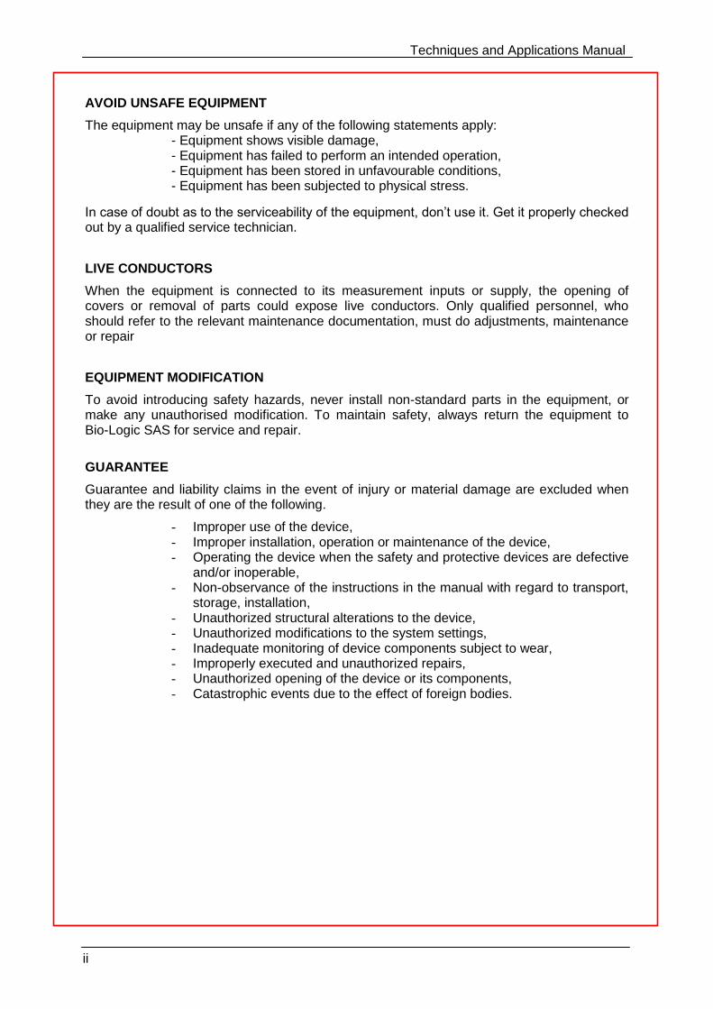
- The serial number of the device located on the rear panel device.
- The software and hardware version you are currently using. On the Help menu, click About. The displayed dialog box shows the version numbers.
- The operating system on the connected computer. - The connection mode (Ethernet, LAN, USB) between computer and
instrument.
Model: SP-150 s/n°: 0001 Power: 110-240 Vac 50/60 Hz Fuses: 10 AF Pmax: 650 W
Techniques and Applications Manual
iv
General safety considerations
Class I
The instrument is safety ground to the Earth through the protective conductor of the AC power cable.
Use only the power cord supplied with the instrument and designed for the good current rating (10 A max) and be sure to connect it to a power source provided with protective earth contact.
Any interruption of the protective earth (grounding) conductor outside the instrument could result in personal injury.
Guarantee and liability claims in the event of injury or material damage are excluded when they are the result of one of the following.
- Improper use of the device, - Improper installation, operation or maintenance of the
device, - Operating the device when the safety and protective
devices are defective and/or inoperable, - Non-observance of the instructions in the manual with
regard to transport, storage, installation, - Unauthorised structural alterations to the device, - Unauthorised modifications to the system settings, - Inadequate monitoring of device components subject
to wear, - Improperly executed and unauthorised repairs, - Unauthorised opening of the device or its components, - Catastrophic events due to the effect of foreign bodies.
ONLY QUALIFIED PERSONNEL should operate (or service) this equipment.
Techniques and Applications Manual
1
Table of contents
Equipment installation ................................................................................................ i General description .................................................................................................... i Intended use of the equipment ................................................................................... i Instructions for use ..................................................................................................... i General safety considerations .................................................................................. iv
1. Introduction........................................................................................................................ 3
2. Voltamperometric techniques ........................................................................................... 4
2.1 OCV: Open Circuit Voltage ....................................................................................... 4
2.2 CV: Cyclic Voltammetry ............................................................................................. 5
2.2.1 CV: Standard Cyclic Voltammetry ............................................................................ 5 2.2.2 CV Linear: Linear Cyclic Voltammetry ...................................................................... 8
2.3 CA: Chronoamperometry ........................................................................................ 10
2.3.1 CA Standard .......................................................................................................... 10 2.3.2 CA Adv: Advanced Chronoamperometry ................................................................ 12 2.3.3 CA Fast: Fast Chronoamperometry ........................................................................ 13
2.4 CP: Chronopotentiometry ........................................................................................ 15
2.4.1 CP Standard .......................................................................................................... 15 2.4.2 CP Adv: Advanced Chronopotentiometry ............................................................... 16 2.4.3 CP Fast: Fast Chronopotentiometry ....................................................................... 18
2.5 PDyn: Potentiodynamic ........................................................................................... 19
2.5.1 Standard Potendynamic: PDyn .............................................................................. 19 2.5.2 Potendynamic Advanced: PDyn Adv ...................................................................... 21
2.6 GDyn: Galvanodynamic .......................................................................................... 22
2.6.1 Standard Galvanodynamic: GDyn .......................................................................... 22 2.6.2 Galvanodynamic Advanced: GDyn Adv .................................................................. 25
2.7 LASV: Large Amplitude Sinusoidal Voltammetry ..................................................... 27
2.8 MOD: Modular Pulse ............................................................................................... 28
2.8.1 Potentiostatic Mode ................................................................................................ 29 2.8.2 Galvanostatic Mode ............................................................................................... 30
3. Electrochemical Impedance Spectroscopy ................................................................... 32
3.1 PEIS: Potentio Electrochemical Impedance Spectroscopy ...................................... 32
3.2 GEIS: Galvano Electrochemical Impedance Spectroscopy ..................................... 34
3.2.1 Visualisation of impedance data files ..................................................................... 35 3.2.2 Frequency vs. time plot .......................................................................................... 36
3.3 SPEIS: Staircase Potentio Electrochemical Impedance Spectroscopy .................... 38
3.4 SGEIS: Staircase Galvano Electrochemical Impedance Spectroscopy ................... 41
4. Pulsed techniques ........................................................................................................... 44
4.1 DPV: Differential Pulse Voltammetry ....................................................................... 44
4.2 SWV: Square Wave Voltammetry ........................................................................... 47
4.3 NPV: Normal Pulse Voltammetry ............................................................................ 49
4.4 RNPV: Reverse Normal Pulse Voltammetry ............................................................ 51
4.5 DNPV: Differential Normal Pulse Voltammetry ........................................................ 53
4.6 DPA: Differential Pulse Amperometry ...................................................................... 55
Techniques and Applications Manual
2
5. STACK techniques .......................................................................................................... 58
5.1 Stack PDYN: Potentiodynamic measurement on a stack ........................................ 59
5.2 Stack GDYN: Galvanodynamic measurement on a stack ........................................ 60
5.3 Stack PEIS: Potentiostatic Impedance on stacks .................................................... 62
5.4 Stack GEIS: Galvanostatic Impedance on stacks .................................................... 65
6. Corrosion techniques ...................................................................................................... 67
6.1 EVT: Ecorr versus Time ............................................................................................ 67
6.2 LP: Linear Polarization ............................................................................................ 68
6.3 GC: Generalized Corrosion ..................................................................................... 70
6.4 CPP: Cyclic Potentiodynamic Polarization ............................................................... 72
6.5 PDP: Potentiodynamic Pitting .................................................................................. 74
6.6 PSP: Potentiostatic Pitting ....................................................................................... 76
6.7 ZRA: Zero Resistance Ammeter .............................................................................. 77
6.8 CASG: Constant Amplitude sinusoidal micro-Galvanopolarisation .......................... 79
6.9 Constant Amplitude Sinusoidal microPolarization (CASP) ....................................... 81
6.10 Variable Amplitude Sinusoidal microPolarization (VASP) ........................................ 82
7. Ohmic Drop Determination ............................................................................................. 85
7.1 MIR: Manual IR ....................................................................................................... 85
7.2 PZIR: IR determination with Potentio Impedance Spectroscopy .............................. 85
7.3 GZIR: IR determination with Galvanostatic Impedance ........................................... 87
7.3.1 compensation mode hardware vs software ............................................................ 88 7.3.2 Ohmic drop compensation ..................................................................................... 88
8. Triggers ............................................................................................................................ 89
8.1 Trigger out: TO ........................................................................................................ 89
8.2 Trigger in: TI ............................................................................................................ 90
8.3 Trigger set: TOS ...................................................................................................... 90
9. Multiplexer ....................................................................................................................... 92
10. Bipot ............................................................................................................................. 95
10.1 CV_CA : CV synchronized with CA ......................................................................... 95
10.2 CP_CA : CP synchronized with CA ......................................................................... 98
10.3 CA_CA : CA synchonized with CA ........................................................................ 100
11. The Loop option ......................................................................................................... 104
12. Combined techniques: .............................................................................................. 105
13. Minimum acquisition time calculation ...................................................................... 106
14. Glossary ..................................................................................................................... 109
15. Acronyms list ............................................................................................................. 112
16. Index ........................................................................................................................... 114
Techniques and Applications Manual
3
1. Introduction
EC-Lab Express software has been designed to control single channel potentiostats (SP-50, SP-150, SP-200, SP-240, SP-300 and HCP803). But it is also compatible with the other potentiostats of our range (VMP2(Z), BiStat, VMP3, VSP and VSP-300). Each channel board of our multichannel instruments is an independent potentiostat/galvanostat that can be
controlled by EC-Lab Express software.
The application software package provides useful techniques. They are separated into nine sections: voltamperometric techniques (Cyclic Voltammetry, Chrono-methods,…), impedance techniques, pulsed techniques, stack techniques, corrosion techniques, Ohmic drop techniques, multiplexer techniques and bipotentiostat techniques. Most of these techniques can contain several sequences (for example pulses). Complex experiments are obtained by associations of linked elementary techniques and appear in the experiment frame.
The aim of this manual is to describe every technique available in EC-Lab Express software. This manual is composed up of several chapters. After the introduction, each field will be described. An additional section will detail the way to build complex experiments as linked techniques.
It is assumed that the user is familiar with Microsoft Windows©
and knows how to use the
mouse and keyboard to access the drop-down menus.
WHEN A USER RECEIVES A NEW UNIT FROM THE FACTORY, THE SOFTWARE AND FIRMWARE ARE
INSTALLED AND UPGRADED. THE INSTRUMENT IS READY TO BE USED. IT DOES NOT NEED TO BE
UPGRADED. WE ADVISE THE USERS TO READ AT LEAST THE FIRST THREE CHAPTERS BEFORE
STARTING AN EXPERIMENT.
Techniques and Applications Manual
4
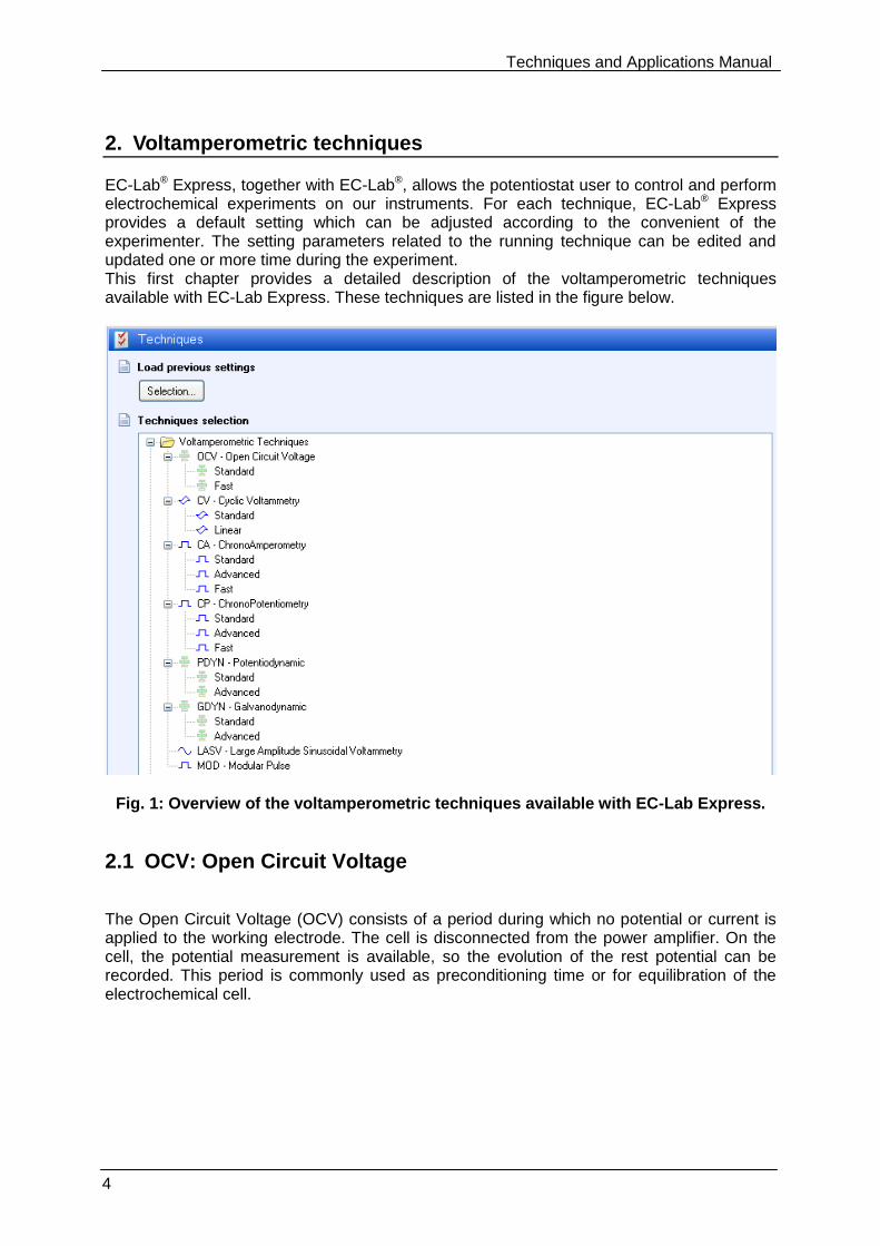
2. Voltamperometric techniques
EC-Lab® Express, together with EC-Lab®, allows the potentiostat user to control and perform electrochemical experiments on our instruments. For each technique, EC-Lab® Express provides a default setting which can be adjusted according to the convenient of the experimenter. The setting parameters related to the running technique can be edited and updated one or more time during the experiment. This first chapter provides a detailed description of the voltamperometric techniques available with EC-Lab Express. These techniques are listed in the figure below.
Fig. 1: Overview of the voltamperometric techniques available with EC-Lab Express.
2.1 OCV: Open Circuit Voltage
The Open Circuit Voltage (OCV) consists of a period during which no potential or current is applied to the working electrode. The cell is disconnected from the power amplifier. On the cell, the potential measurement is available, so the evolution of the rest potential can be recorded. This period is commonly used as preconditioning time or for equilibration of the electrochemical cell.
Techniques and Applications Manual
5
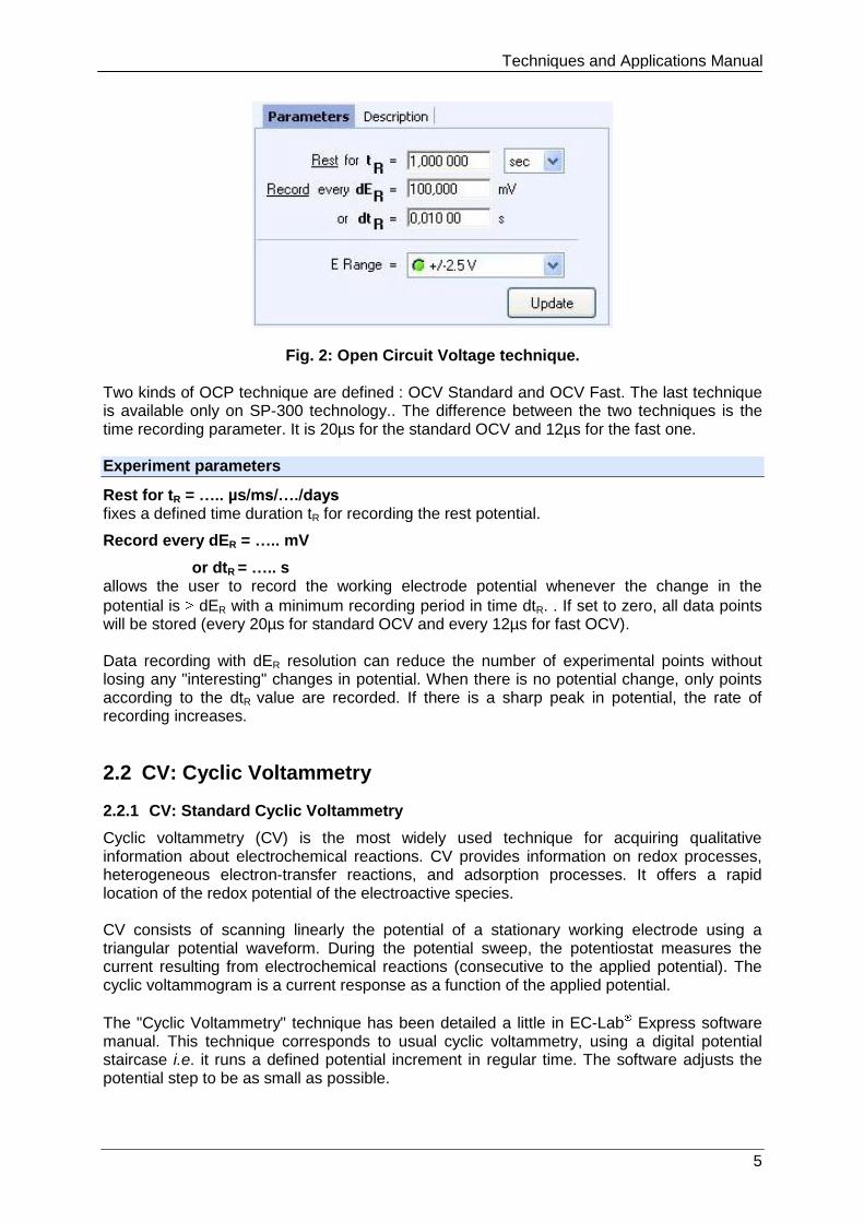
Fig. 2: Open Circuit Voltage technique. Two kinds of OCP technique are defined : OCV Standard and OCV Fast. The last technique is available only on SP-300 technology.. The difference between the two techniques is the time recording parameter. It is 20µs for the standard OCV and 12µs for the fast one. Experiment parameters
Rest for tR = ….. µs/ms/…./days fixes a defined time duration tR for recording the rest potential.
Record every dER = ….. mV
or dtR = ….. s allows the user to record the working electrode potential whenever the change in the
potential is dER with a minimum recording period in time dtR. . If set to zero, all data points will be stored (every 20µs for standard OCV and every 12µs for fast OCV). Data recording with dER resolution can reduce the number of experimental points without losing any "interesting" changes in potential. When there is no potential change, only points according to the dtR value are recorded. If there is a sharp peak in potential, the rate of recording increases.
2.2 CV: Cyclic Voltammetry
2.2.1 CV: Standard Cyclic Voltammetry
Cyclic voltammetry (CV) is the most widely used technique for acquiring qualitative information about electrochemical reactions. CV provides information on redox processes, heterogeneous electron-transfer reactions, and adsorption processes. It offers a rapid location of the redox potential of the electroactive species. CV consists of scanning linearly the potential of a stationary working electrode using a triangular potential waveform. During the potential sweep, the potentiostat measures the current resulting from electrochemical reactions (consecutive to the applied potential). The cyclic voltammogram is a current response as a function of the applied potential.
The "Cyclic Voltammetry" technique has been detailed a little in EC-Lab Express software manual. This technique corresponds to usual cyclic voltammetry, using a digital potential staircase i.e. it runs a defined potential increment in regular time. The software adjusts the potential step to be as small as possible.
Techniques and Applications Manual
6
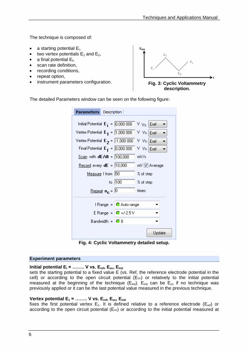
The technique is composed of:
a starting potential Ei,
two vertex potentials E1 and E2,
a final potential Ef,
scan rate definition,
recording conditions,
repeat option,
instrument parameters configuration.
Fig. 3: Cyclic Voltammetry
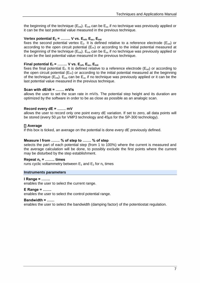
description. The detailed Parameters window can be seen on the following figure:
Fig. 4: Cyclic Voltammetry detailed setup.
Experiment parameters
Initial potential Ei = …….. V vs. Eref, Eoc, Einit sets the starting potential to a fixed value E (vs. Ref, the reference electrode potential in the cell) or according to the open circuit potential (Eoc) or relatively to the initial potential measured at the beginning of the technique (Einit). Einit can be Eoc if no technique was previously applied or it can be the last potential value measured in the previous technique. Vertex potential E1 = …….. V vs. Eref, Eoc, Einit fixes the first potential vertex E1. It is defined relative to a reference electrode (Eref) or according to the open circuit potential (Eoc) or according to the initial potential measured at
Techniques and Applications Manual
7
the beginning of the technique (Einit). Einit can be Eoc if no technique was previously applied or it can be the last potential value measured in the previous technique. Vertex potential E2 = …….. V vs. Eref, Eoc, Einit fixes the second potential vertex E2. It is defined relative to a reference electrode (Eref) or according to the open circuit potential (Eoc) or according to the initial potential measured at the beginning of the technique (Einit). Einit can be Eoc if no technique was previously applied or it can be the last potential value measured in the previous technique. Final potential Ef = …….. V vs. Eref, Eoc, Einit fixes the final potential Ef. It is defined relative to a reference electrode (Eref) or according to the open circuit potential (Eoc) or according to the initial potential measured at the beginning of the technique (Einit). Einit can be Eoc if no technique was previously applied or it can be the last potential value measured in the previous technique. Scan with dE/dt = ……. mV/s allows the user to set the scan rate in mV/s. The potential step height and its duration are optimized by the software in order to be as close as possible as an analogic scan.
Record every dE = ……. mV allows the user to record only one point every dE variation. If set to zero, all data points will be stored (every 50 µs for VMP3 technology and 45µs for the SP-300 technology). [] Average if this box is ticked, an average on the potential is done every dE previously defined.
Measure I from ……. % of step to ……. % of step selects the part of each potential step (from 1 to 100%) where the current is measured and the average calculation will be done, to possibly exclude the first points where the current may be disturbed by the step establishment.
Repeat nc = …….. times runs cyclic voltammetry between E1 and E2 for nc times Instruments parameters
I Range = ……. enables the user to select the current range.
E Range = ……. enables the user to select the control potential range.
Bandwidth = …… enables the user to select the bandwidth (damping factor) of the potentiostat regulation.
Techniques and Applications Manual
8
2.2.2 CV Linear: Linear Cyclic Voltammetry
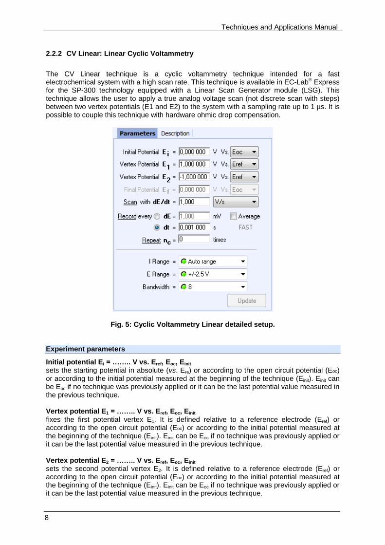
The CV Linear technique is a cyclic voltammetry technique intended for a fast electrochemical system with a high scan rate. This technique is available in EC-Lab® Express for the SP-300 technology equipped with a Linear Scan Generator module (LSG). This technique allows the user to apply a true analog voltage scan (not discrete scan with steps) between two vertex potentials (E1 and E2) to the system with a sampling rate up to 1 µs. It is possible to couple this technique with hardware ohmic drop compensation.
Fig. 5: Cyclic Voltammetry Linear detailed setup. Experiment parameters
Initial potential Ei = …….. V vs. Eref, Eoc, Einit sets the starting potential in absolute (vs. Ere) or according to the open circuit potential (Eoc) or according to the initial potential measured at the beginning of the technique (Einit). Einit can be Eoc if no technique was previously applied or it can be the last potential value measured in the previous technique. Vertex potential E1 = …….. V vs. Eref, Eoc, Einit fixes the first potential vertex E1. It is defined relative to a reference electrode (Eref) or according to the open circuit potential (Eoc) or according to the initial potential measured at the beginning of the technique (Einit). Einit can be Eoc if no technique was previously applied or it can be the last potential value measured in the previous technique. Vertex potential E2 = …….. V vs. Eref, Eoc, Einit sets the second potential vertex E2. It is defined relative to a reference electrode (Eref) or according to the open circuit potential (Eoc) or according to the initial potential measured at the beginning of the technique (Einit). Einit can be Eoc if no technique was previously applied or it can be the last potential value measured in the previous technique.
Techniques and Applications Manual
9
Final potential Ef = …….. V vs. Eref, Eoc, Einit (disabled) The Final potential Ef is disabled. Its value is automatically settled at Ei potential (Ef=Ei). Scan with dE/dt = ……. mV/s, mV/min, V/s, KV/s allows the user to set the scan rate in mV/s The potential step height and its duration are optimized by the software in order to be as close as possible as an analogic scan.
Record every dE = ……. mV (or dt = ……. s, optional)
allows the possibility to record I with two conditions on potential variation dE or on time variation dt. The two conditions cannot be entered simultaneously. If the dt parameter set to zero all data points will be stored every 15µs. [] Average if this box is ticked, an average on the potential is done every dE previously defined. For acquisition time lower than 15µs this box is disabled. Repeat option for cycling
Repeat nc = …….. times run cyclic voltammetry between E1 and E2 for nc times. Instruments parameters
I Range = ……. enables the user to select the current range.
E Range = ……. enables the user to select the control potential range.
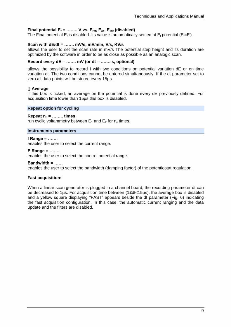
Bandwidth = …… enables the user to select the bandwidth (damping factor) of the potentiostat regulation. Fast acquisition: When a linear scan generator is plugged in a channel board, the recording parameter dt can be decreased to 1µs. For acquisition time between (1≤dt<15µs), the average box is disabled and a yellow square displaying “FAST” appears beside the dt parameter (Fig. 6) indicating the fast acquisition configuration. In this case, the automatic current ranging and the data update and the filters are disabled.
Techniques and Applications Manual
10
Fig. 6: Fast Cyclic Voltammetry setup.
2.3 CA: Chronoamperometry
2.3.1 CA Standard
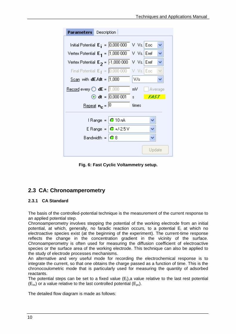
The basis of the controlled-potential technique is the measurement of the current response to an applied potential step. Chronoamperometry involves stepping the potential of the working electrode from an initial potential, at which, generally, no faradic reaction occurs, to a potential Ei at which no electroactive species exist (at the beginning of the experiment). The current-time response reflects the change in the concentration gradient in the vicinity of the surface. Chronoamperometry is often used for measuring the diffusion coefficient of electroactive species or the surface area of the working electrode. This technique can also be applied to the study of electrode processes mechanisms. An alternative and very useful mode for recording the electrochemical response is to integrate the current, so that one obtains the charge passed as a function of time. This is the chronocoulometric mode that is particularly used for measuring the quantity of adsorbed reactants. The potential steps can be set to a fixed value (Ei),a value relative to the last rest potential (Eoc) or a value relative to the last controlled potential (Epc). The detailed flow diagram is made as follows:
Techniques and Applications Manual
11
potential step,
potential sequences,
recording conditions,
repeat option,
instrument parameters configuration.
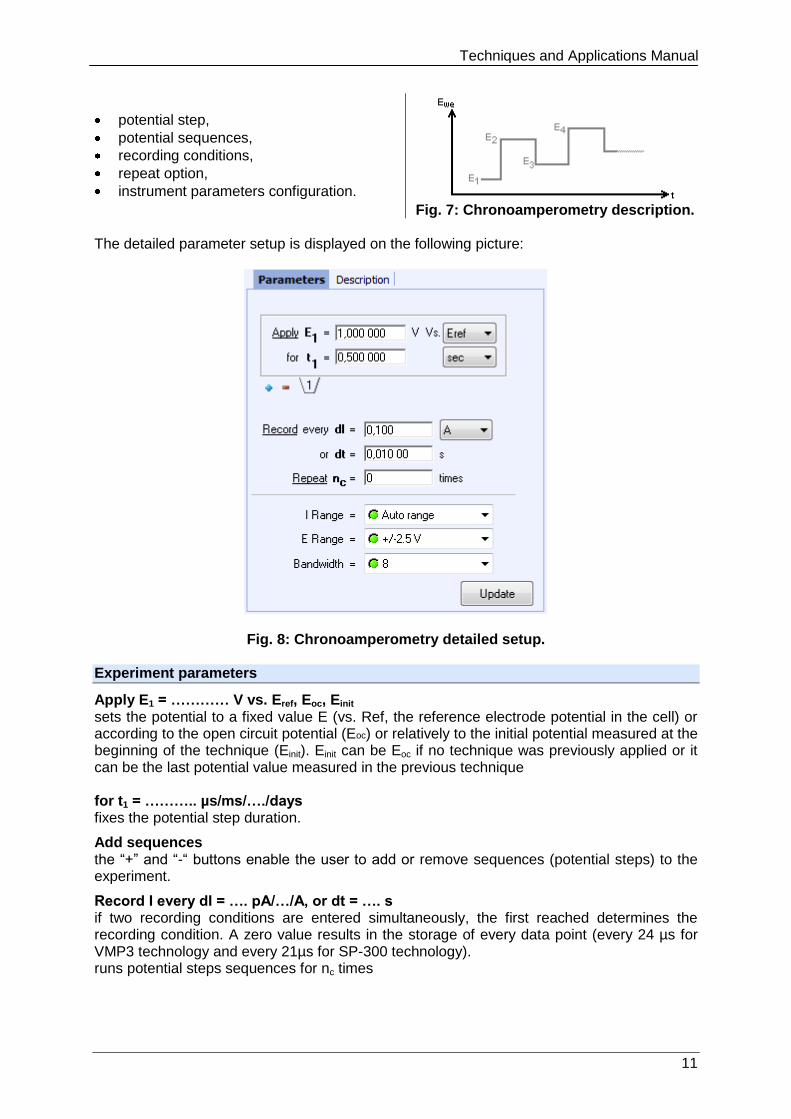
Fig. 7: Chronoamperometry description.
The detailed parameter setup is displayed on the following picture:
Fig. 8: Chronoamperometry detailed setup.
Experiment parameters
Apply E1 = ………… V vs. Eref, Eoc, Einit sets the potential to a fixed value E (vs. Ref, the reference electrode potential in the cell) or according to the open circuit potential (Eoc) or relatively to the initial potential measured at the beginning of the technique (Einit). Einit can be Eoc if no technique was previously applied or it can be the last potential value measured in the previous technique for t1 = ……….. µs/ms/…./days fixes the potential step duration.
Add sequences the “+” and “-“ buttons enable the user to add or remove sequences (potential steps) to the experiment.
Record I every dI = …. pA/…/A, or dt = …. s if two recording conditions are entered simultaneously, the first reached determines the recording condition. A zero value results in the storage of every data point (every 24 µs for VMP3 technology and every 21µs for SP-300 technology). runs potential steps sequences for nc times
Techniques and Applications Manual
12
Instruments parameters
I Range = ……. enables the user to select the current range.
E Range = ……. enables the user to select the control potential range.
Bandwidth = …… enables the user to select the bandwidth (damping factor) of the potentiostat regulation.
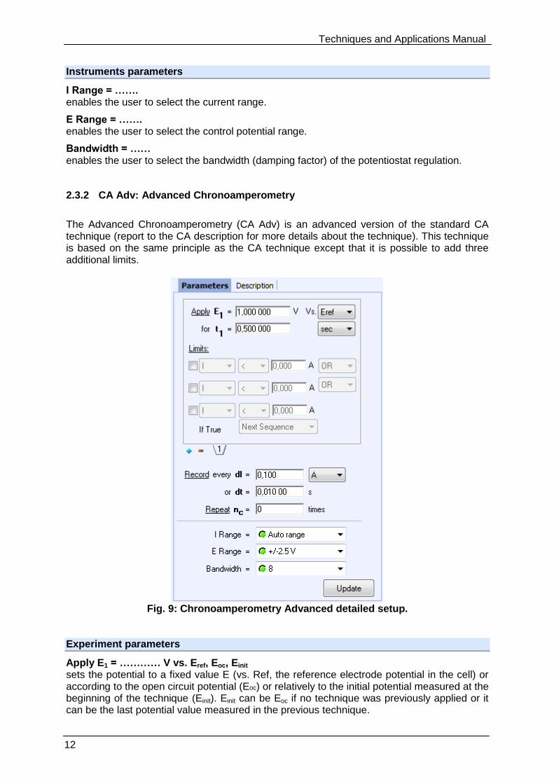
2.3.2 CA Adv: Advanced Chronoamperometry
The Advanced Chronoamperometry (CA Adv) is an advanced version of the standard CA technique (report to the CA description for more details about the technique). This technique is based on the same principle as the CA technique except that it is possible to add three additional limits.
Fig. 9: Chronoamperometry Advanced detailed setup.
Experiment parameters
Apply E1 = ………… V vs. Eref, Eoc, Einit sets the potential to a fixed value E (vs. Ref, the reference electrode potential in the cell) or according to the open circuit potential (Eoc) or relatively to the initial potential measured at the beginning of the technique (Einit). Einit can be Eoc if no technique was previously applied or it can be the last potential value measured in the previous technique.
Techniques and Applications Manual
13
for t1 = ……….. µs/ms/…./days fixes the potential step duration. Limits: I/IN1/IN2/Q </> ....... A/C OR/AND defines a limit on current or on IN1 or on IN2 or on charge Q and the sign of this limit. AND function allows adding different limits, each of them should be reached to go to next step. OR function allows selecting one limit among the other and to go to the next step when reached. If True Next Sequence/ Next Technique/ Stop Experiment defines the action to do when limit(s) is (are) reached.
Add sequences the “+” and “-“ buttons enable the user to add or remove sequences (potential steps) to the experiment.
Record I every dI = …. pA/…/A, or dt = …. s if two recording conditions are entered simultaneously, the first reached determines the recoding. A zero value results in the storage of every data point (every 40µs for VMP3 technology and every 34µs for SP-300 technology).
Repeat nc = …….. times runs potential steps sequences for nc times Instruments parameters
I Range = ……. enables the user to select the current range.
E Range = ……. enables the user to select the control potential range.
Bandwidth = …… enables the user to select the bandwidth (damping factor) of the potentiostat regulation.
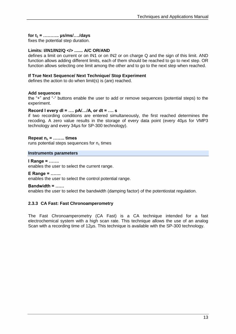
2.3.3 CA Fast: Fast Chronoamperometry
The Fast Chronoamperometry (CA Fast) is a CA technique intended for a fast electrochemical system with a high scan rate. This technique allows the use of an analog Scan with a recording time of 12µs. This technique is available with the SP-300 technology.
Techniques and Applications Manual
14
Fig. 10: Fast Chronoamperometry detailed setup. Experiment parameters
Apply E1 = ………… V vs. Eref, Eoc, Einit sets the potential to a fixed value E (vs. Ref, the reference electrode potential in the cell) or according to the open circuit potential (Eoc) or relatively to the initial potential measured at the beginning of the technique (Einit). Einit can be Eoc if no technique was previously applied or it can be the last potential value measured in the previous technique. For t1 = ……….. µs/ms/…./days fixes the potential step duration.
Add sequences the “+” and “-“ buttons enable the user to add or remove sequences (potential steps) to the experiment.
Record I every dI = …. pA/…/A, or dt = …. s if two recording conditions are entered simultaneously, the first reached determines the recoding. A zero value results in the storage of every data point (every 14µs).
Repeat nc = …….. times runs potential steps sequences for nc times Instruments parameters
I Range = ……. enables the user to select the current range.
E Range = ……. enables the user to select the control potential range.
Bandwidth = ……
Techniques and Applications Manual
15
enables the user to select the bandwidth (damping factor) of the potentiostat regulation.
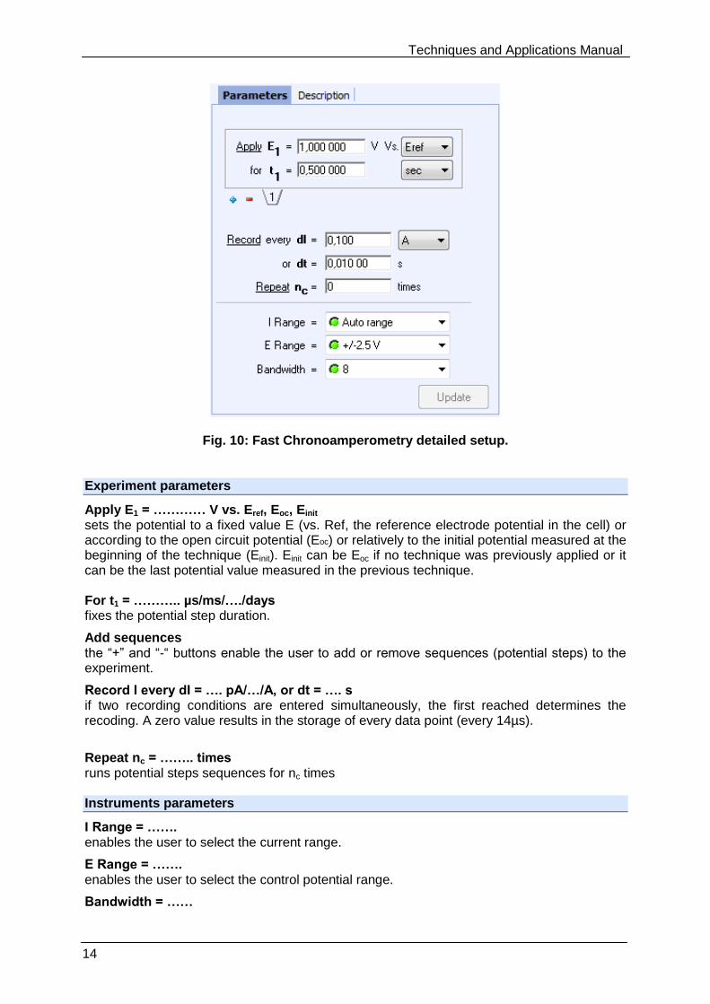
2.4 CP: Chronopotentiometry
2.4.1 CP Standard
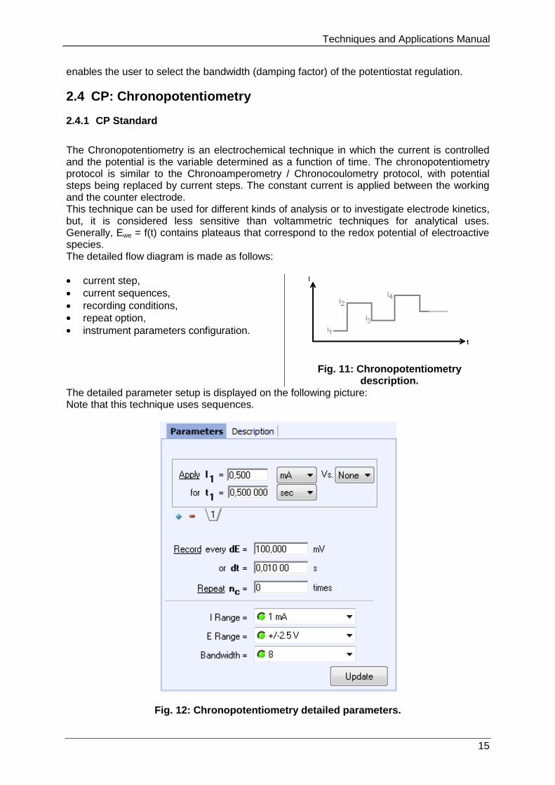
The Chronopotentiometry is an electrochemical technique in which the current is controlled and the potential is the variable determined as a function of time. The chronopotentiometry protocol is similar to the Chronoamperometry / Chronocoulometry protocol, with potential steps being replaced by current steps. The constant current is applied between the working and the counter electrode. This technique can be used for different kinds of analysis or to investigate electrode kinetics, but, it is considered less sensitive than voltammetric techniques for analytical uses. Generally, Ewe = f(t) contains plateaus that correspond to the redox potential of electroactive species. The detailed flow diagram is made as follows:
current step,
current sequences,
recording conditions,
repeat option,
instrument parameters configuration.
Fig. 11: Chronopotentiometry description.
The detailed parameter setup is displayed on the following picture: Note that this technique uses sequences.
Fig. 12: Chronopotentiometry detailed parameters.
Techniques and Applications Manual
16
Experiment parameters
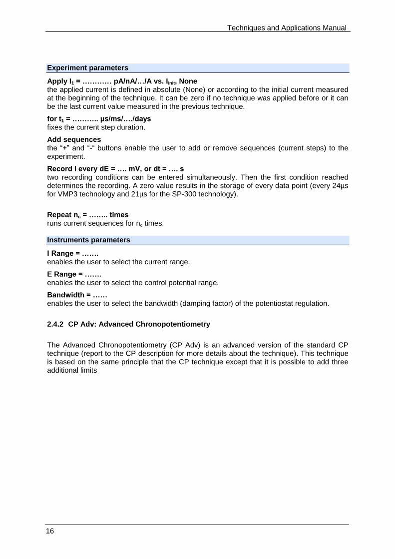
Apply I1 = ………… pA/nA/…/A vs. Iinit, None the applied current is defined in absolute (None) or according to the initial current measured at the beginning of the technique. It can be zero if no technique was applied before or it can be the last current value measured in the previous technique.
for t1 = ……….. µs/ms/…./days fixes the current step duration.
Add sequences the “+” and “-“ buttons enable the user to add or remove sequences (current steps) to the experiment.
Record I every dE = …. mV, or dt = …. s two recording conditions can be entered simultaneously. Then the first condition reached determines the recording. A zero value results in the storage of every data point (every 24µs for VMP3 technology and 21µs for the SP-300 technology).
Repeat nc = …….. times runs current sequences for nc times. Instruments parameters
I Range = ……. enables the user to select the current range.
E Range = ……. enables the user to select the control potential range.
Bandwidth = …… enables the user to select the bandwidth (damping factor) of the potentiostat regulation.
2.4.2 CP Adv: Advanced Chronopotentiometry
The Advanced Chronopotentiometry (CP Adv) is an advanced version of the standard CP technique (report to the CP description for more details about the technique). This technique is based on the same principle that the CP technique except that it is possible to add three additional limits
Techniques and Applications Manual
17
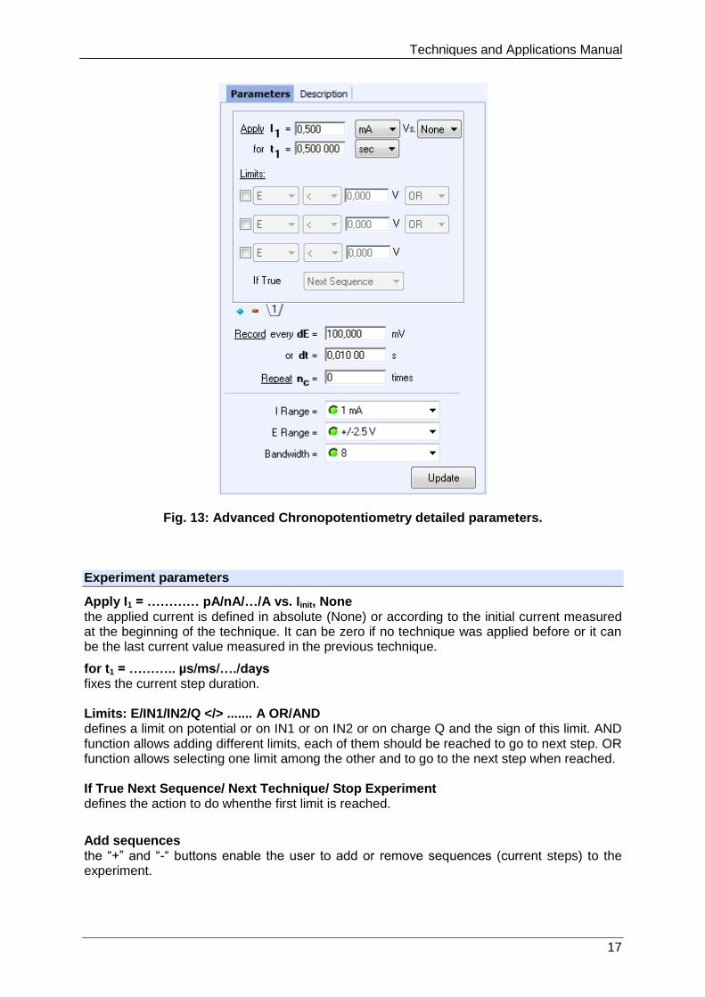
Fig. 13: Advanced Chronopotentiometry detailed parameters.
Experiment parameters
Apply I1 = ………… pA/nA/…/A vs. Iinit, None the applied current is defined in absolute (None) or according to the initial current measured at the beginning of the technique. It can be zero if no technique was applied before or it can be the last current value measured in the previous technique.
for t1 = ……….. µs/ms/…./days fixes the current step duration. Limits: E/IN1/IN2/Q </> ....... A OR/AND defines a limit on potential or on IN1 or on IN2 or on charge Q and the sign of this limit. AND function allows adding different limits, each of them should be reached to go to next step. OR function allows selecting one limit among the other and to go to the next step when reached. If True Next Sequence/ Next Technique/ Stop Experiment defines the action to do whenthe first limit is reached.
Add sequences the “+” and “-“ buttons enable the user to add or remove sequences (current steps) to the experiment.
Techniques and Applications Manual
18
Record I every dE = …. mV, or dt = …. s two recording conditions can be entered simultaneously. Then the first condition reached determines the recording. A zero value results in the storage of every data point (every 40 µs for VMP3 technology and 34µs for the SP-300 technology).
Repeat nc = …….. times runs current sequences for nc times. Instruments parameters
I Range = ……. enables the user to select the current range.
E Range = ……. enables the user to select the control potential range.
Bandwidth = …… enables the user to select the bandwidth (damping factor) of the potentiostat regulation.
2.4.3 CP Fast: Fast Chronopotentiometry
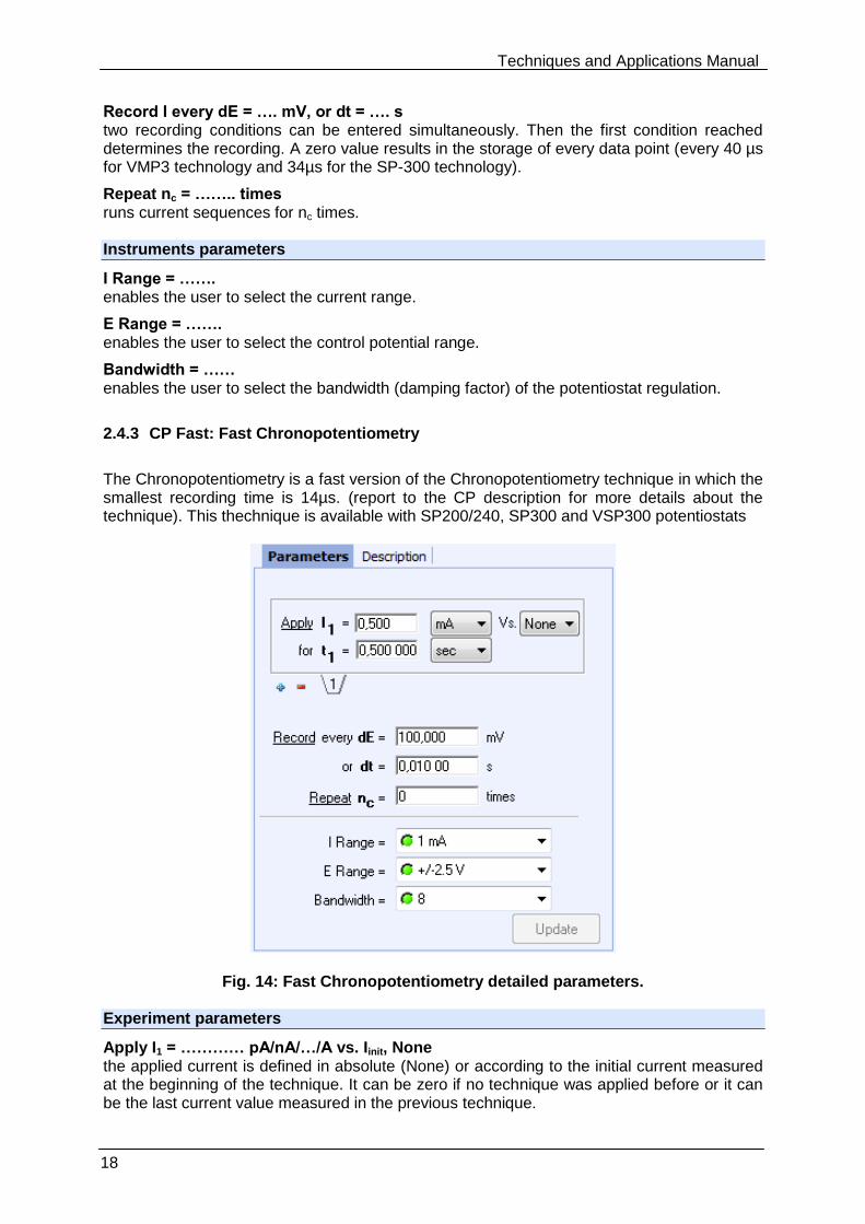
The Chronopotentiometry is a fast version of the Chronopotentiometry technique in which the smallest recording time is 14µs. (report to the CP description for more details about the technique). This thechnique is available with SP200/240, SP300 and VSP300 potentiostats
Fig. 14: Fast Chronopotentiometry detailed parameters. Experiment parameters
Apply I1 = ………… pA/nA/…/A vs. Iinit, None the applied current is defined in absolute (None) or according to the initial current measured at the beginning of the technique. It can be zero if no technique was applied before or it can be the last current value measured in the previous technique.
Techniques and Applications Manual
19
for t1 = ……….. µs/ms/…./days
fixes the current step duration.
Add sequences the “+” and “-“ buttons enable the user to add or remove sequences (current steps) to the experiment.
Record I every dE = …. mV, or dt = …. s two recording conditions can be entered simultaneously. Then the first condition reached determines the recording. A zero value results in the storage of every data point (every 14 µs).
Repeat nc = …….. times runs current sequences for nc times. Instruments parameters
I Range = ……. enables the user to select the current range.
E Range = ……. enables the user to select the control potential range.
Bandwidth = …… enables the user to select the bandwidth (damping factor) of the potentiostat regulation.
2.5 PDyn: Potentiodynamic
2.5.1 Standard Potendynamic: PDyn
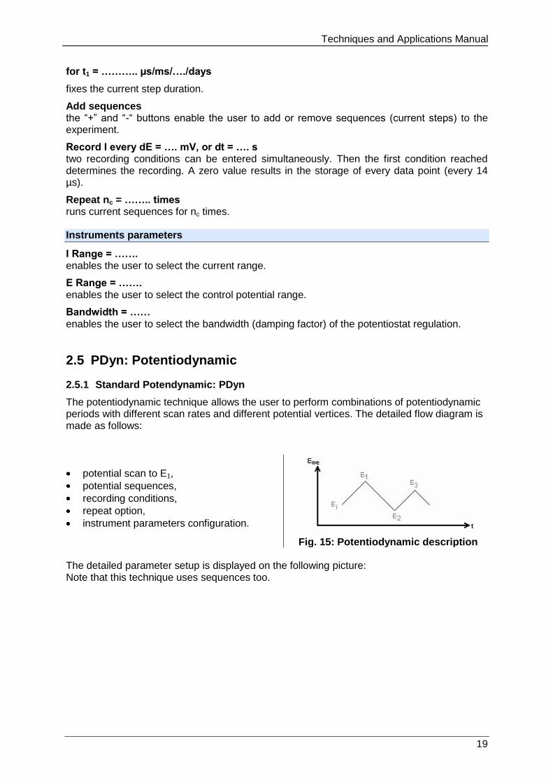
The potentiodynamic technique allows the user to perform combinations of potentiodynamic periods with different scan rates and different potential vertices. The detailed flow diagram is made as follows:
potential scan to E1,
potential sequences,
recording conditions,
repeat option,
instrument parameters configuration.
Fig. 15: Potentiodynamic description The detailed parameter setup is displayed on the following picture: Note that this technique uses sequences too.
Techniques and Applications Manual
20
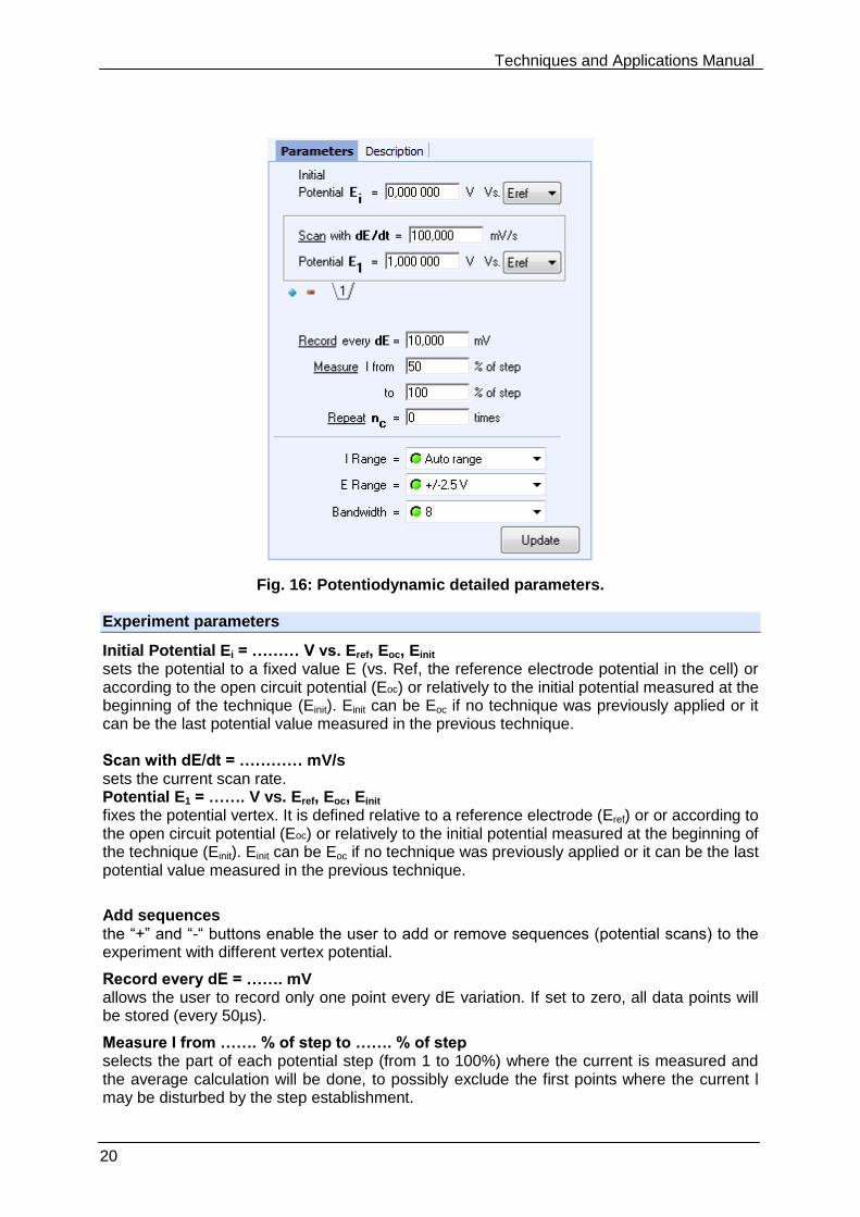
Fig. 16: Potentiodynamic detailed parameters. Experiment parameters
Initial Potential Ei = ……… V vs. Eref, Eoc, Einit sets the potential to a fixed value E (vs. Ref, the reference electrode potential in the cell) or according to the open circuit potential (Eoc) or relatively to the initial potential measured at the beginning of the technique (Einit). Einit can be Eoc if no technique was previously applied or it can be the last potential value measured in the previous technique. Scan with dE/dt = ………… mV/s sets the current scan rate. Potential E1 = ……. V vs. Eref, Eoc, Einit fixes the potential vertex. It is defined relative to a reference electrode (Eref) or or according to the open circuit potential (Eoc) or relatively to the initial potential measured at the beginning of the technique (Einit). Einit can be Eoc if no technique was previously applied or it can be the last potential value measured in the previous technique.
Add sequences the “+” and “-“ buttons enable the user to add or remove sequences (potential scans) to the experiment with different vertex potential.
Record every dE = ……. mV allows the user to record only one point every dE variation. If set to zero, all data points will be stored (every 50µs).
Measure I from ……. % of step to ……. % of step selects the part of each potential step (from 1 to 100%) where the current is measured and the average calculation will be done, to possibly exclude the first points where the current l may be disturbed by the step establishment.
Techniques and Applications Manual
21
Repeat nc = …….. times runs potential scan sequences for nc times. Instruments parameters
I Range = ……. enables the user to select the current range.
E Range = ……. enables the user to select the control potential range.
Bandwidth = …… enables the user to select the bandwidth (damping factor) of the potentiostat regulation.
2.5.2 Potendynamic Advanced: PDyn Adv
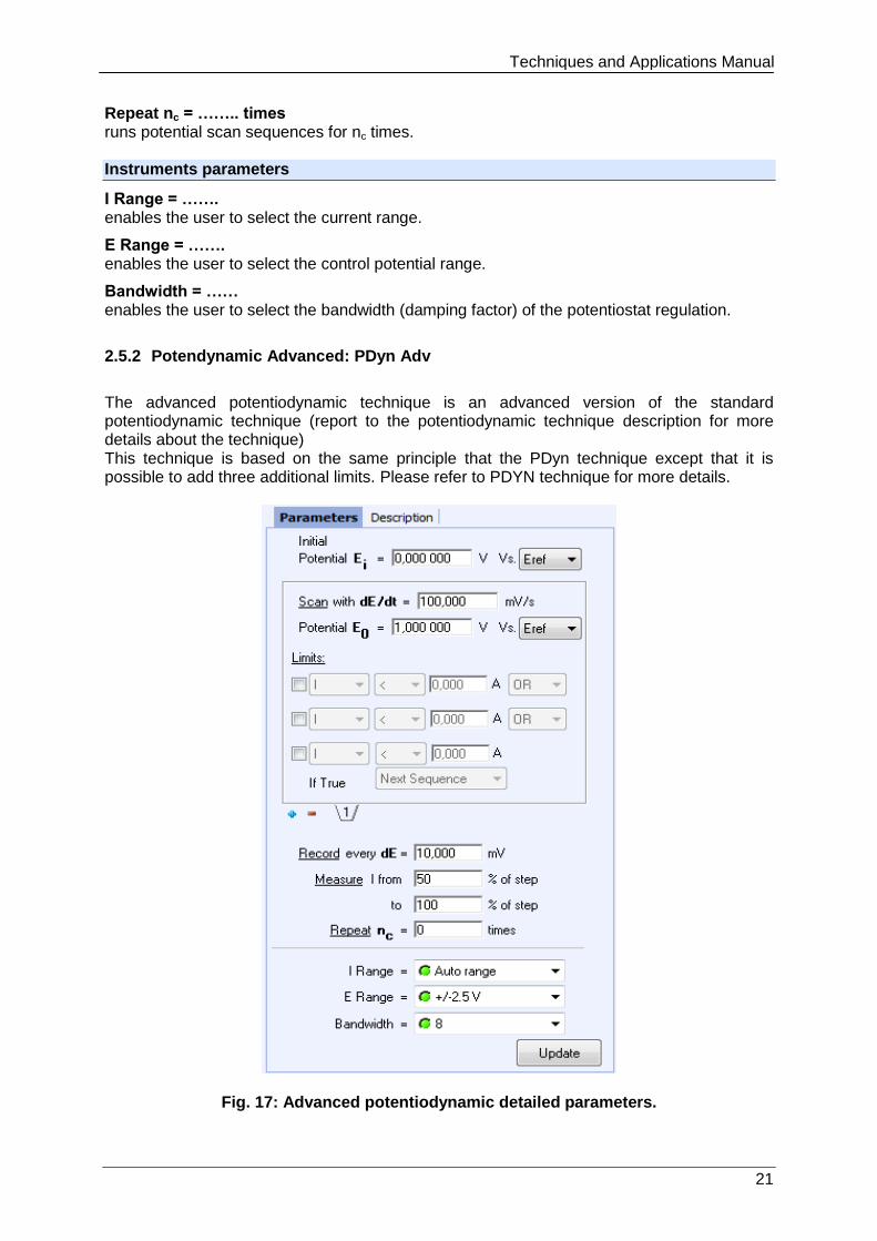
The advanced potentiodynamic technique is an advanced version of the standard potentiodynamic technique (report to the potentiodynamic technique description for more details about the technique) This technique is based on the same principle that the PDyn technique except that it is possible to add three additional limits. Please refer to PDYN technique for more details.
Fig. 17: Advanced potentiodynamic detailed parameters.
Techniques and Applications Manual
22
Experiment parameters
Initial Potential Ei = ……… V vs. Eref, Eoc, Einit sets the initial potential Ei to a fixed value E (vs. Ref, the reference electrode potential in the cell) or according to the open circuit potential (Eoc) or according to the initial potential measured at the beginning of the technique (Einit). Einit can be Eoc if no technique was previously applied or it can be the last potential value measured in the previous technique. Scan with dE/dt = ………… mV/s sets the current scan rate.
Potential E1 = ……. V vs. Eref, Eoc, Einit fixes the potential vertex E1. It is defined relative to a reference electrode (Eref) or or according to the open circuit potential (Eoc) or relatively to the initial potential measured at the beginning of the technique (Einit). Einit can be Eoc if no technique was previously applied or it can be the last potential value measured in the previous technique. Limits: I/IN1/IN2/Q </> ....... A/C OR/AND defines a limit on current or on IN1 or on IN2 or on charge Q and the sign of this limit. AND function allows adding different limits, each of them should be reached to go to next step. OR function allows selecting one limit among the other and to go to the next step when reached. If True Next Sequence/ Next Technique/ Stop Experiment defines the action to do when the limit is reached.
Add sequences the “+” and “-“ buttons enable the user to add or remove sequences (potential scans) to the experiment with different vertex potential.
Record every dE = ……. mV allows the user to record only one point every dE variation. If set to zero, all data points will be stored (every 60 µs).
Measure I from ……. % of step to ……. % of step selects the part of each potential step (from 1 to 100%) where the current is measured and the average calculation will be done, to possibly exclude the first points where the current l may be disturbed by the step establishment.
Repeat nc = …….. times runs potential scan sequences for nc times. Instruments parameters
I Range = ……. enables the user to select the current range.
E Range = ……. enables the user to select the control potential range.
Bandwidth = …… enables the user to select the bandwidth (damping factor) of the potentiostat regulation.
2.6 GDyn: Galvanodynamic
2.6.1 Standard Galvanodynamic: GDyn
Techniques and Applications Manual
23
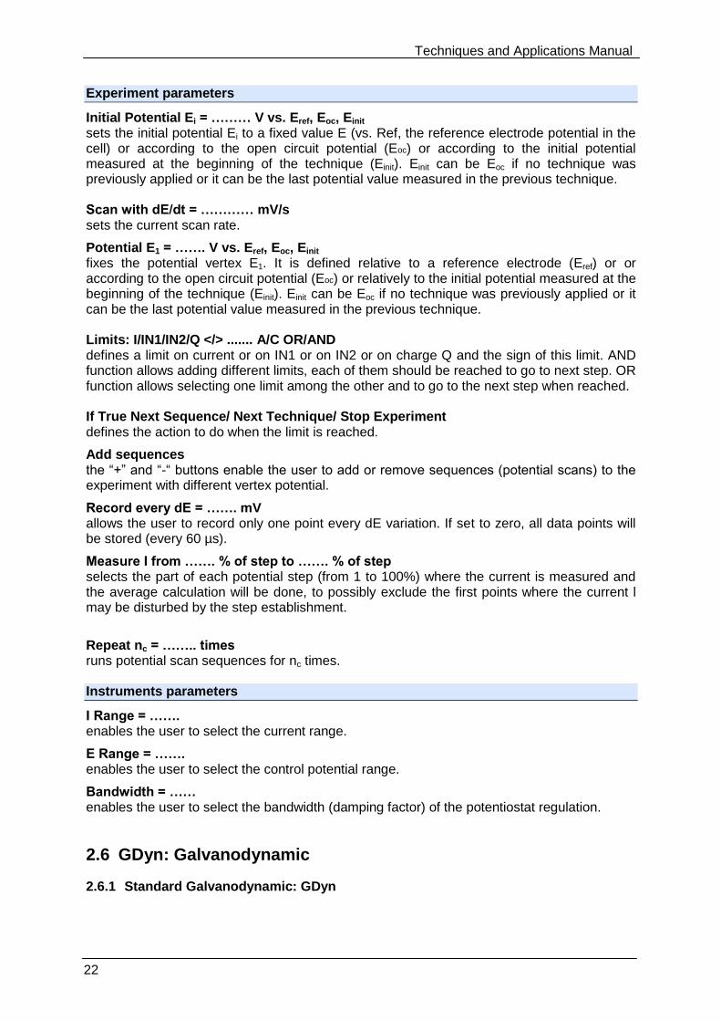
The Galvanodynamic technique allows the user to perform combinations of galvanodynamic periods with different scan rates and different current vertex. The detailed flow diagram is made as follows:
current scan to I1,
current sequences,
recording conditions,
repeat option,
instrument parameters configuration.
Fig. 18: Galvanodynamic description.
The detailed parameter setup is displayed on the following picture:
Fig. 19: Galvanodynamic detailed parameters. Experiment parameters
Initial Current Ii = ……… pA/nA/…/A vs. Iinit, None fixes the starting current Ii. It is defined in absolute (None) or according to the initial current measured at the beginning of the technique. It can be zero if no technique was applied before or it can be the last current value measured in the previous technique. Scan with dI/dt = …………A/s, mA/s, µA/s, nA/s, pA/s sets the current scan rate.
Techniques and Applications Manual
24
Current I1 = ……. pA/nA/…/A vs. Iinit, None fixes the current vertex I1. It is defined in absolute (None) or according to the initial current measured at the beginning of the technique (Iinit). It can be 0 if no technique was previously applied, or it can be the last current value measured in the previous technique.
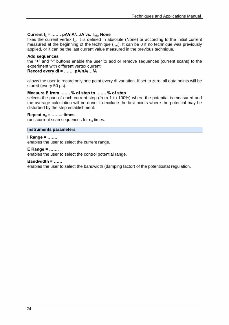
Add sequences the “+” and “-“ buttons enable the user to add or remove sequences (current scans) to the experiment with different vertex current. Record every dI = ……. pA/nA/…/A allows the user to record only one point every dI variation. If set to zero, all data points will be stored (every 50 µs).
Measure E from ……. % of step to ……. % of step selects the part of each current step (from 1 to 100%) where the potential is measured and the average calculation will be done, to exclude the first points where the potential may be disturbed by the step establishment.
Repeat nc = …….. times runs current scan sequences for nc times. Instruments parameters
I Range = ……. enables the user to select the current range.
E Range = ……. enables the user to select the control potential range.
Bandwidth = …… enables the user to select the bandwidth (damping factor) of the potentiostat regulation.
Techniques and Applications Manual
25
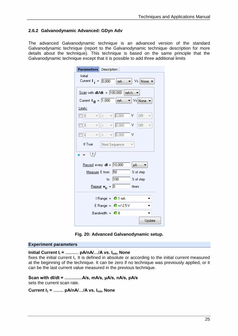
2.6.2 Galvanodynamic Advanced: GDyn Adv
The advanced Galvanodynamic technique is an advanced version of the standard Galvanodynamic technique (report to the Galvanodynamic technique description for more details about the technique). This technique is based on the same principle that the Galvanodynamic technique except that it is possible to add three additional limits
Fig. 20: Advanced Galvanodynamic setup. Experiment parameters
Initial Current Ii = ……… pA/nA/…/A vs. Iinit, None fixes the initial current Ii. It is defined in absolute or according to the initial current measured at the beginning of the technique. It can be zero if no technique was previously applied, or it can be the last current value measured in the previous technique. Scan with dI/dt = …………A/s, mA/s, µA/s, nA/s, pA/s sets the current scan rate.
Current I1 = ……. pA/nA/…/A vs. Iinit, None
Techniques and Applications Manual
26
fixes the current vertex I1. It is defined in absolute or according to the initial current measured at the beginning of the technique. It can be 0 if no technique was previously applied, or it can be the last current value measured in the previous technique. Limits: E/IN1/IN2/Q </> ....... A/C OR/AND defines a limit on potential or on IN1 or on IN2 or on charge Q and the sign of this limit. AND function allows adding different limits, each of them should be reached to go to next step. OR function allows selecting one limit among the other and to go to the next step when reached. If True Next Sequence/ Next Technique/ Stop Experiment defines the action to do when the first limit is reached.
Add sequences the “+” and “-“ buttons enable the user to add or remove sequences (current scans) to the experiment with different vertex current. Record every dI = ……. pA/nA/…/A allows the user to record only one point every dI variation. If set to zero, all data points will be stored (every 60 µs).
Measure E from ……. % of step to ……. % of step selects the part of each current step (from 1 to 100%) where the potential is measured and the average calculation will be done, to exclude the first points where the potential may be disturbed by the step establishment.
Repeat nc = …….. times runs current scan sequences for nc times. Instruments parameters
I Range = ……. enables the user to select the current range.
E Range = ……. enables the user to select the control potential range.
Bandwidth = …… enables the user to select the bandwidth (damping factor) of the potentiostat regulation.
Techniques and Applications Manual
27
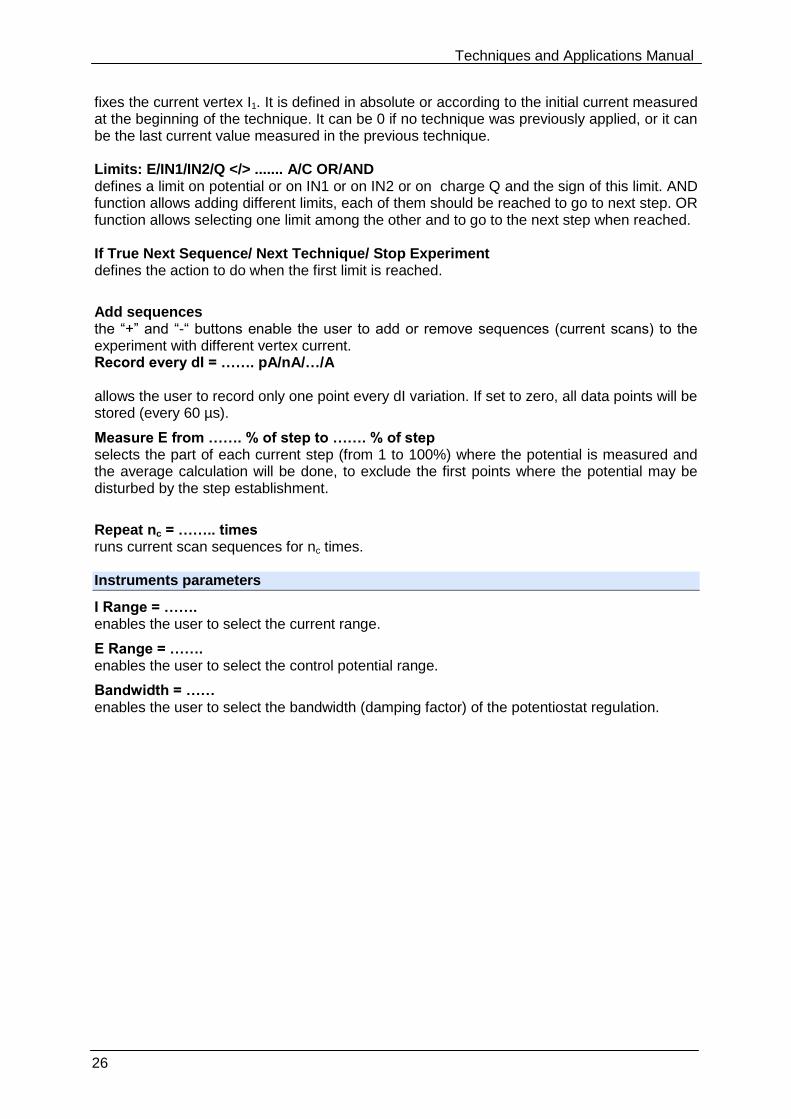
2.7 LASV: Large Amplitude Sinusoidal Voltammetry
Large Amplitude Sinusoidal Voltammetry (LASV) is an electrochemical technique where the potential excitation of the working electrode is a large amplitude sinusoidal waveform. Similar to the cyclic voltammetry (CV) technique, it gives qualitative and quantitative information on the redox processes. In contrast to the CV, the double layer capacitive current is not subject to sharp transitions at reverse potentials. As the electrochemical systems are non-linear the current response exhibits high order harmonics at large sinusoidal amplitudes. Valuable information can be found from data analysis in the frequency domain. The technique is composed of:
a starting potential,
a frequency definition fs,
a potential range definition from E1 to E2,
the possibility to repeat np times potential scan.
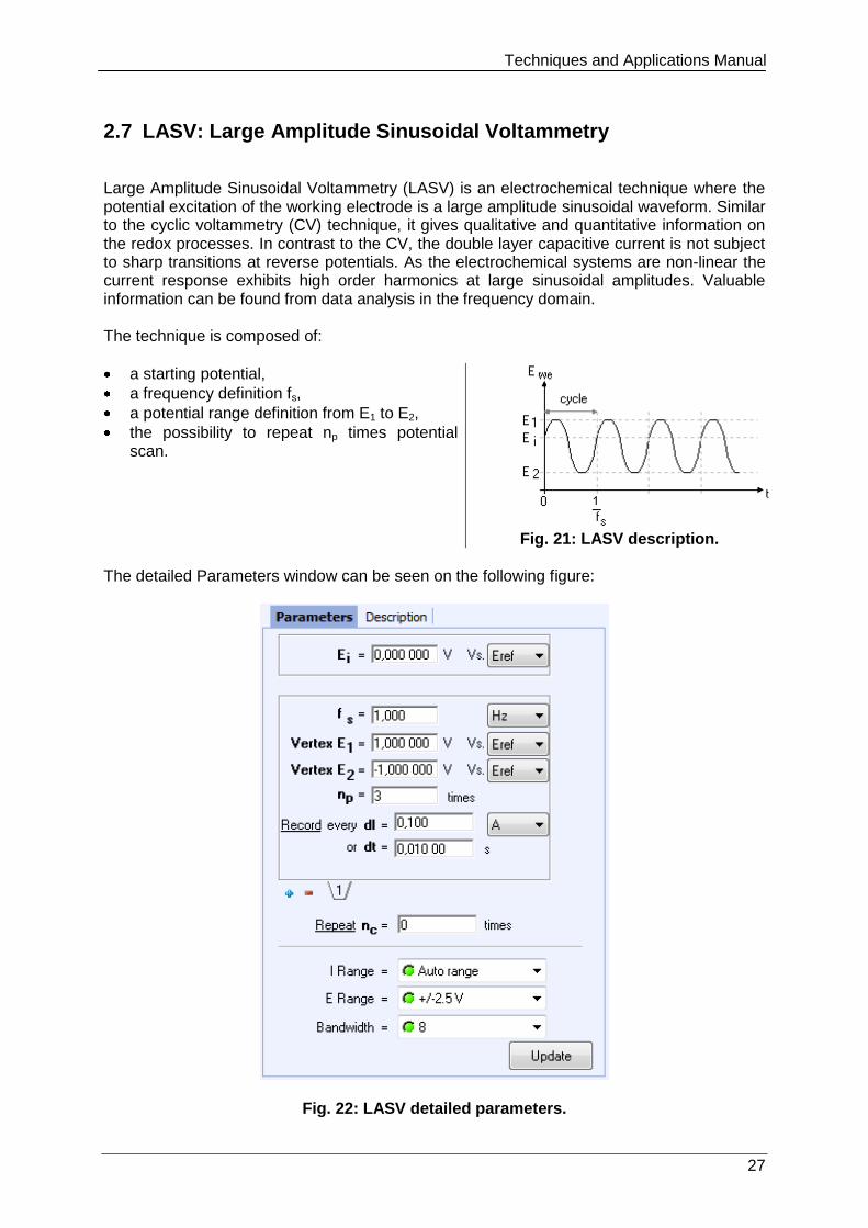
Fig. 21: LASV description. The detailed Parameters window can be seen on the following figure:
Fig. 22: LASV detailed parameters.
Techniques and Applications Manual
28
Experiment parameters
Initial potential Ei = …….. V vs. Eref, Eoc, Einit sets the potential to a fixed value E (vs. Ref, the reference electrode potential in the cell) or according to the open circuit potential (Eoc) or relatively to the initial potential measured at the beginning of the technique (Einit). Einit can be Eoc if no technique was previously applied or it can be the last potential value measured in the previous technique. fs = ..... MHz/kHz/Hz/mHz/µHz allows the user to set the value of frequency which will define the scan rate.
E1 = …….. V vs. Eref, Eoc, Einit fixes the first potential vertex E1. It is defined relative to a reference electrode (Eref) or according to the open circuit potential (Eoc) or relatively to the initial potential measured at the beginning of the technique (Einit). Einit can be Eoc if no technique was previously applied or it can be the last potential value measured in the previous technique.
E2 = …….. V vs. Eref, Eoc, Einit sets E2 vertex potential. It is defined relative to a reference electrode (Eref) or according to the open circuit potential (Eoc) or relatively to the initial potential measured at the beginning of the technique (Einit). Einit can be Eoc if no technique was previously applied or it can be the last potential value measured in the previous technique.
Repeat np = …….. times runs LASV technique between E1 and E2 for np times Record every dI = ….. pA/nA/…/A and dt = ….. s offers the possibility to record I with two conditions on the current variation dI and (or) on time variation. If set to zero, all data points will be stored (every 50 µs). Instruments parameters
Repeat nc = …….. times repeats all the sequences nc times. I Range = ……. enables the user to select the current range.
E Range = ……. enables the user to select the control potential range.
Bandwidth = …… enables the user to select the bandwidth (damping factor) of the potentiostat regulation. Note: for this technique, recording conditions could be defined independently for each sequence.
2.8 MOD: Modular Pulse
The Modular pulse technique (MOD) allows the user to control successively in different sequences the current or the voltage of the cell. This technique can include galvanostatic and potentiostatic sequences. The switch from one sequence to the other is very fast. The recording conditions included in the sequence (rc) offer the possibility to record only few
Techniques and Applications Manual
29
sequences in a long time experiment. This technique is particularly useful for electrochemical coating. Two kind of sequence can be used in the same experiment: potentiostatic sequence and galvanostatic sequence.
2.8.1 Potentiostatic Mode
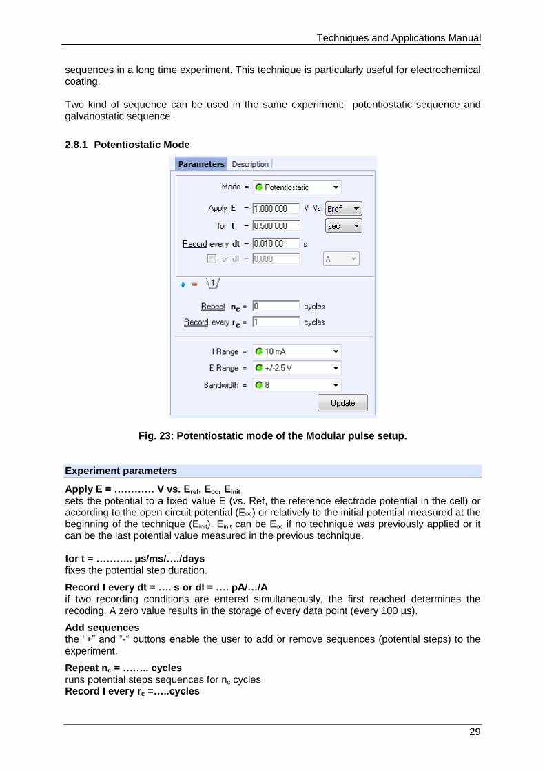
Fig. 23: Potentiostatic mode of the Modular pulse setup. Experiment parameters
Apply E = ………… V vs. Eref, Eoc, Einit sets the potential to a fixed value E (vs. Ref, the reference electrode potential in the cell) or according to the open circuit potential (Eoc) or relatively to the initial potential measured at the beginning of the technique (Einit). Einit can be Eoc if no technique was previously applied or it can be the last potential value measured in the previous technique. for t = ……….. µs/ms/…./days fixes the potential step duration.
Record I every dt = …. s or dI = …. pA/…/A if two recording conditions are entered simultaneously, the first reached determines the recoding. A zero value results in the storage of every data point (every 100 µs).
Add sequences the “+” and “-“ buttons enable the user to add or remove sequences (potential steps) to the experiment.
Repeat nc = …….. cycles runs potential steps sequences for nc cycles Record I every rc =…..cycles
Techniques and Applications Manual
30
The recording parameter rc allows the user to record only few sequences in a long time experiment. During an experiment with nc cycles, the rc satisfy 1 ≤ rc ≤ nc +1 Instruments parameters
I Range = ……. enables the user to select the current range.
E Range = ……. enables the user to select the control potential range.
Bandwidth = …… enables the user to select the bandwidth (damping factor) of the potentiostat regulation.
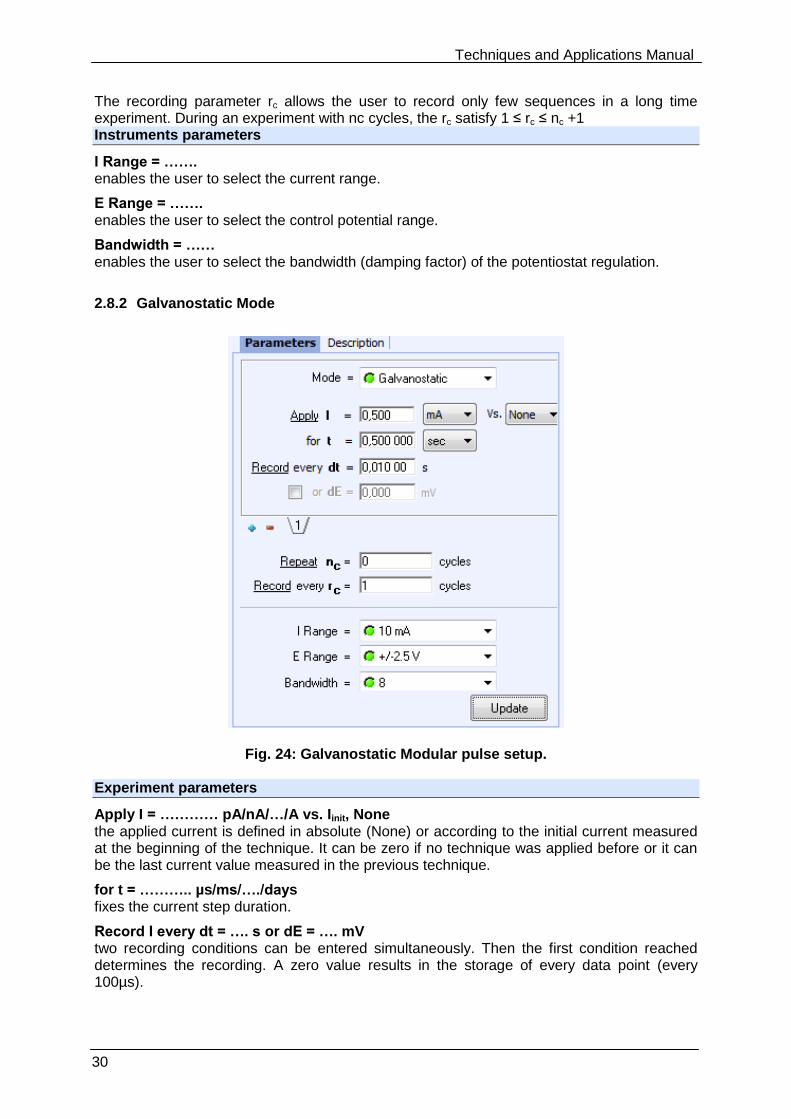
2.8.2 Galvanostatic Mode
Fig. 24: Galvanostatic Modular pulse setup. Experiment parameters
Apply I = ………… pA/nA/…/A vs. Iinit, None the applied current is defined in absolute (None) or according to the initial current measured at the beginning of the technique. It can be zero if no technique was applied before or it can be the last current value measured in the previous technique.
for t = ……….. µs/ms/…./days fixes the current step duration.
Record I every dt = …. s or dE = …. mV two recording conditions can be entered simultaneously. Then the first condition reached determines the recording. A zero value results in the storage of every data point (every 100µs).
Techniques and Applications Manual
31
Add sequences the “+” and “-“ buttons enable the user to add or remove sequences (current steps) to the experiment.
Repeat nc = …….. cycles runs current sequences for nc cycles. Record I every rc =…..cycles The recording parameter rc allows the user to record only few sequences in a long time experiment. During an experiment with nc cycles, the rc satisfy 1 ≤ rc ≤ nc +1 Instruments parameters
I Range = ……. enables the user to select the current range.
E Range = ……. enables the user to select the control potential range.
Bandwidth = …… enables the user to select the bandwidth (damping factor) of the potentiostat regulation.
Techniques and Applications Manual
32
3. Electrochemical Impedance Spectroscopy
Among the modern computational techniques, the Electrochemical Impedance Spectroscopy (EIS) is now a powerful tool for examining many chemical and physical processes in solution as well as in solids. EIS finds many applications in corrosion, battery, fuel cell development, sensors and physical electrochemistry and can provide information on reaction parameters, corrosion rates, electrode surfaces porosity, coating, mass transport, and interfacial capacitance measurements. Our instruments equipped with EIS capability can perform impedance measurements from 10 µHz to 1 MHz pour les potentiostat SP-150, VSP, VMP3 (200 kHz for channel boards delivered before July 2005) and from 10µHz to up to 7 MHz for SP-300 technology. With boosters, this high limit is reduced. The SP-50 is not concerned with this section, as this instrument is not EIS capable.
3.1 PEIS: Potentio Electrochemical Impedance Spectroscopy
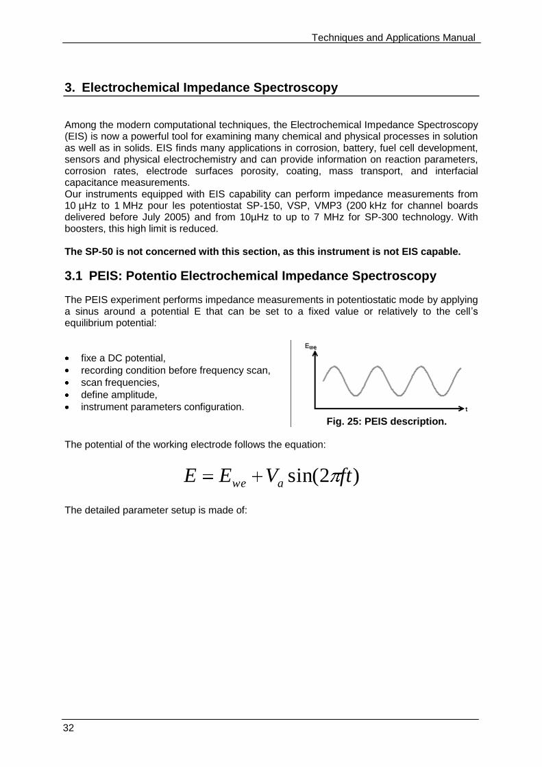
The PEIS experiment performs impedance measurements in potentiostatic mode by applying a sinus around a potential E that can be set to a fixed value or relatively to the cell’s equilibrium potential:
fixe a DC potential,
recording condition before frequency scan,
scan frequencies,
define amplitude,
instrument parameters configuration.
Fig. 25: PEIS description.
The potential of the working electrode follows the equation:
)2sin( ftVEE awe
The detailed parameter setup is made of:
Techniques and Applications Manual
33
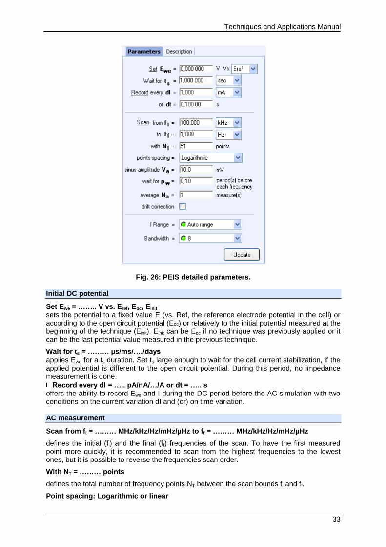
Fig. 26: PEIS detailed parameters. Initial DC potential
Set Ewe = …….. V vs. Eref, Eoc, Einit sets the potential to a fixed value E (vs. Ref, the reference electrode potential in the cell) or according to the open circuit potential (Eoc) or relatively to the initial potential measured at the beginning of the technique (Einit). Einit can be Eoc if no technique was previously applied or it can be the last potential value measured in the previous technique.
Wait for ts = ……… µs/ms/…./days applies Ewe for a ts duration. Set ts large enough to wait for the cell current stabilization, if the applied potential is different to the open circuit potential. During this period, no impedance measurement is done.
Record every dI = ….. pA/nA/…/A or dt = ….. s offers the ability to record Ewe and I during the DC period before the AC simulation with two conditions on the current variation dI and (or) on time variation. AC measurement
Scan from fi = ……… MHz/kHz/Hz/mHz/µHz to ff = ……… MHz/kHz/Hz/mHz/µHz
defines the initial (fi) and the final (ff) frequencies of the scan. To have the first measured point more quickly, it is recommended to scan from the highest frequencies to the lowest ones, but it is possible to reverse the frequencies scan order.
With NT = ……… points
defines the total number of frequency points NT between the scan bounds fi and ff.
Point spacing: Logarithmic or linear
Techniques and Applications Manual
34
defines the point spacing. For example, a scan from fi = 100 kHz to ff = 1 kHz with Nt = 11 total number of points in linear spacing, will make measurements at these frequencies (Hz): 100, 90, 80, 70, 60, 50, 40, 30, 20, 10, 1.
Sinus amplitude Va = …… mV
sets the AC sinus amplitude to Va. It is added to the DC potential level.
Wait for pw = …… period before each frequency
offers the ability to add a delay before the measurement at each frequency. This delay is defined as a part of the period. Of course for low frequencies the delay may be long.
Average Na = ……… mesure(s)
repeats Na measure(s) and average values for each frequency.
Drift correction function resulting in the correction of the DC level drift. This feature is especially dedicated to low frequencies. Note that if this option is selected, the sinus frequencies are evaluated over 2 periods (instead of 1), increasing the acquisition time by a factor of 2. Instruments parameters
I Range = ……. enables the user to select the current range.
Bandwidth = …… enables the user to select the bandwidth (damping factor) of the potentiostat regulation.
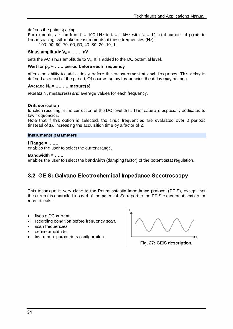
3.2 GEIS: Galvano Electrochemical Impedance Spectroscopy
This technique is very close to the Potentiostastic Impedance protocol (PEIS), except that the current is controlled instead of the potential. So report to the PEIS experiment section for more details.
fixes a DC current,
recording condition before frequency scan,
scan frequencies,
define amplitude,
instrument parameters configuration.
Fig. 27: GEIS description.
Techniques and Applications Manual
35
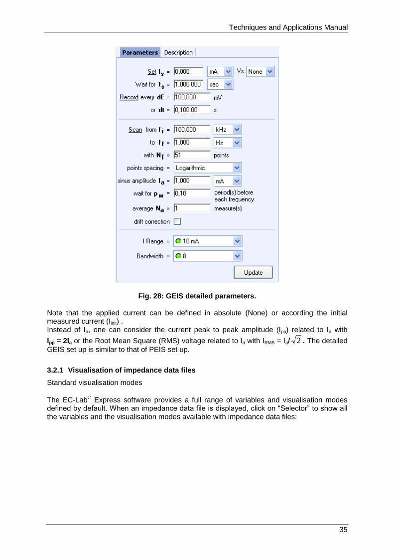
Fig. 28: GEIS detailed parameters. Note that the applied current can be defined in absolute (None) or according the initial measured current (Iinit) . Instead of Ia, one can consider the current peak to peak amplitude (Ipp) related to Ia with
Ipp = 2Ia or the Root Mean Square (RMS) voltage related to Ia with IRMS = Ia/ 2 . The detailed
GEIS set up is similar to that of PEIS set up.
3.2.1 Visualisation of impedance data files
Standard visualisation modes
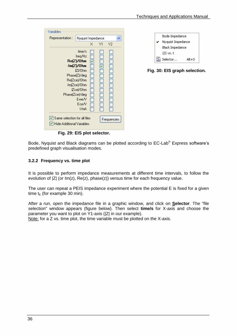
The EC-Lab Express software provides a full range of variables and visualisation modes defined by default. When an impedance data file is displayed, click on “Selector” to show all the variables and the visualisation modes available with impedance data files:
Techniques and Applications Manual
36
Fig. 29: EIS plot selector.
Fig. 30: EIS graph selection.
Bode, Nyquist and Black diagrams can be plotted according to EC-Lab® Express software’s predefined graph visualisation modes.
3.2.2 Frequency vs. time plot
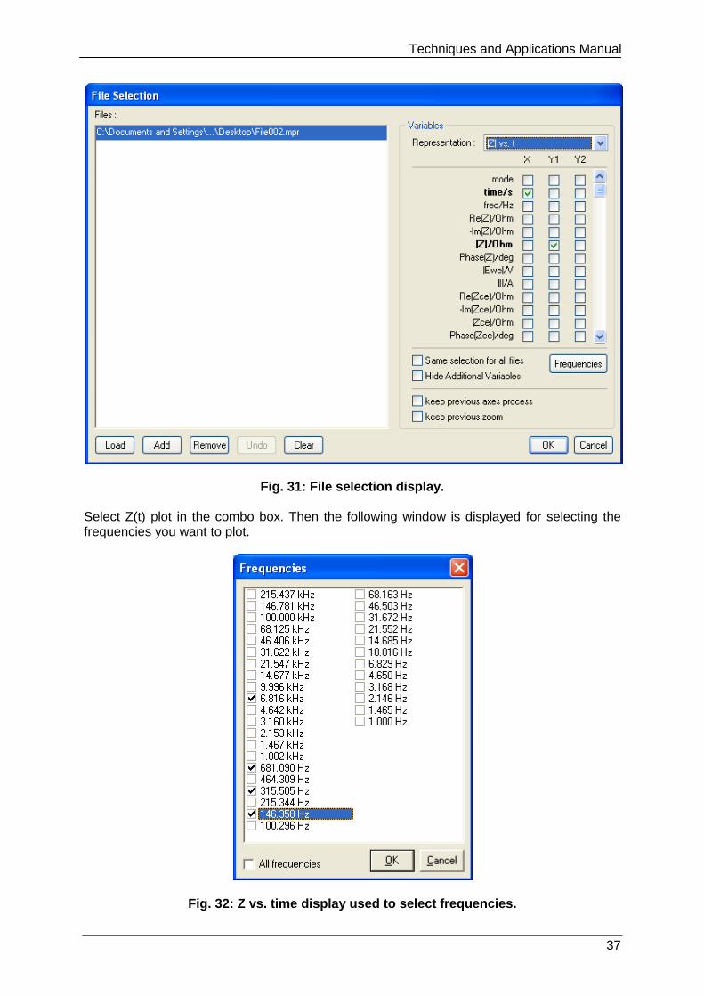
It is possible to perform impedance measurements at different time intervals, to follow the evolution of |Z| (or Im(z), Re(z), phase(z)) versus time for each frequency value. The user can repeat a PEIS impedance experiment where the potential E is fixed for a given time tE (for example 30 min). After a run, open the impedance file in a graphic window, and click on Selector. The "file selection" window appears (figure below). Then select time/s for X-axis and choose the parameter you want to plot on Y1-axis (|Z| in our example). Note: for a Z vs. time plot, the time variable must be plotted on the X-axis.
Techniques and Applications Manual
37
Fig. 31: File selection display. Select Z(t) plot in the combo box. Then the following window is displayed for selecting the frequencies you want to plot.
Fig. 32: Z vs. time display used to select frequencies.
Techniques and Applications Manual
38
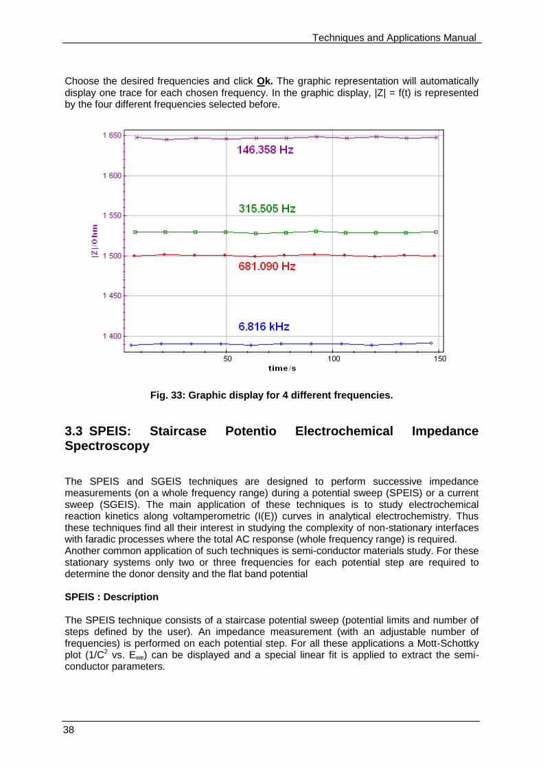
Choose the desired frequencies and click Ok. The graphic representation will automatically display one trace for each chosen frequency. In the graphic display, |Z| = f(t) is represented by the four different frequencies selected before.
Fig. 33: Graphic display for 4 different frequencies.
3.3 SPEIS: Staircase Potentio Electrochemical Impedance Spectroscopy
The SPEIS and SGEIS techniques are designed to perform successive impedance measurements (on a whole frequency range) during a potential sweep (SPEIS) or a current sweep (SGEIS). The main application of these techniques is to study electrochemical reaction kinetics along voltamperometric (I(E)) curves in analytical electrochemistry. Thus these techniques find all their interest in studying the complexity of non-stationary interfaces with faradic processes where the total AC response (whole frequency range) is required. Another common application of such techniques is semi-conductor materials study. For these stationary systems only two or three frequencies for each potential step are required to determine the donor density and the flat band potential SPEIS : Description The SPEIS technique consists of a staircase potential sweep (potential limits and number of steps defined by the user). An impedance measurement (with an adjustable number of frequencies) is performed on each potential step. For all these applications a Mott-Schottky plot (1/C2 vs. Ewe) can be displayed and a special linear fit is applied to extract the semi-conductor parameters.
Techniques and Applications Manual
39
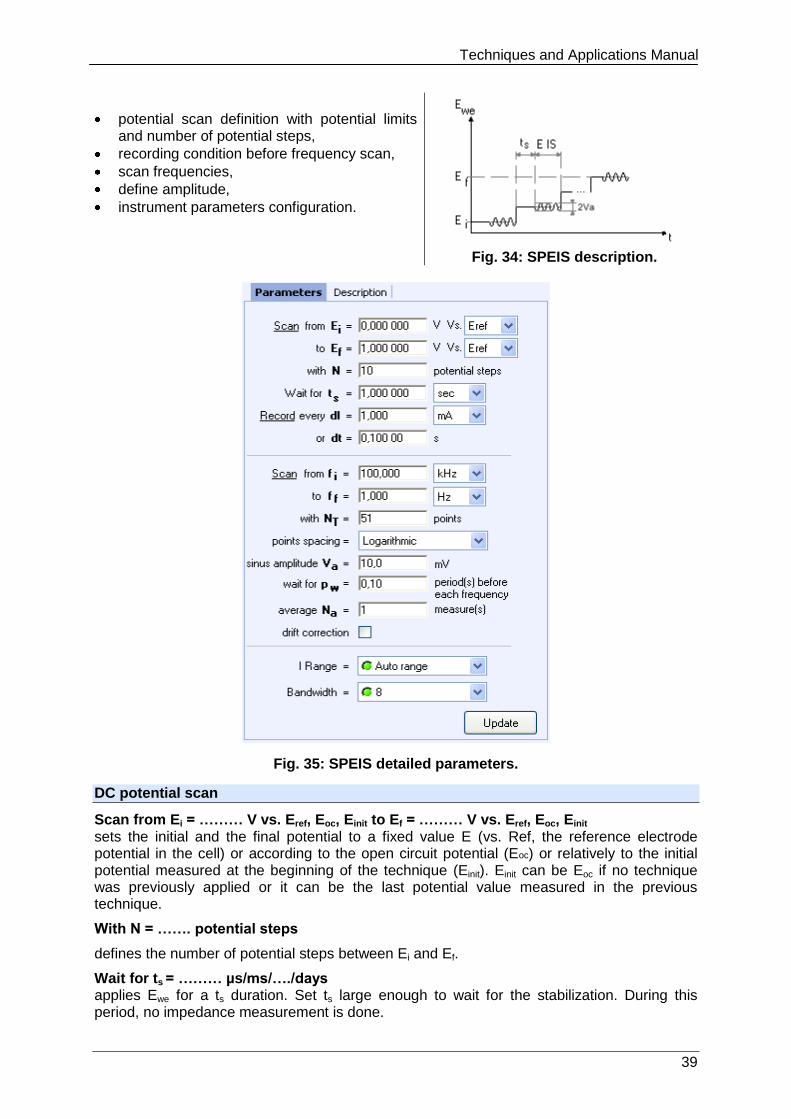
potential scan definition with potential limits and number of potential steps,
recording condition before frequency scan,
scan frequencies,
define amplitude,
instrument parameters configuration.
Fig. 34: SPEIS description.
Fig. 35: SPEIS detailed parameters.
DC potential scan
Scan from Ei = ……… V vs. Eref, Eoc, Einit to Ef = ……… V vs. Eref, Eoc, Einit sets the initial and the final potential to a fixed value E (vs. Ref, the reference electrode potential in the cell) or according to the open circuit potential (Eoc) or relatively to the initial potential measured at the beginning of the technique (Einit). Einit can be Eoc if no technique was previously applied or it can be the last potential value measured in the previous technique.
With N = ……. potential steps
defines the number of potential steps between Ei and Ef.
Wait for ts = ……… µs/ms/…./days applies Ewe for a ts duration. Set ts large enough to wait for the stabilization. During this period, no impedance measurement is done.
Techniques and Applications Manual
40
Record every dI = ….. pA/nA/…./A or dt = ….. s offers the ability to record Ewe and I during the DC period before the AC simulation with two conditions on the current variation dI and (or) on time variation. AC measurement
Scan from fi = ……… MHz/kHz/Hz/mHz/µHz to ff = ……… MHz/kHz/Hz/mHz/µHz
defines the initial (fi) and final (ff) frequencies of the scan. To have the first measured point more quickly, it is recommended to scan from the highest frequencies to the lowest ones, but it is possible to reverse the frequencies scan order.
With NT = ……… points
defines the total number of frequency points NT between the scan bounds fi and ff.
Point spacing: Logarithmic or linear
defines the point spacing. For example, a scan from fi = 100 kHz to ff = 1 kHz with NT = 11 total number of points in linear spacing, will make measurements at these frequencies (Hz): 100, 90, 80, 70, 60, 50, 40, 30, 20, 10, 1. Sinus amplitude Ia = …… pA/nA/…./A sets the AC sinus amplitude to Ea. It is added to the DC potential level.
Wait for pw = …… period before each frequency
offers the ability to add a delay before the measurement at each frequency. This delay is defined as a part of the period. Of course for low frequencies the delay may be long.
Average Na = ……… measure(s)
repeats Na measure(s) and average values for each frequency.
Drift correction
function resulting in the correction of the DC level drift. This feature is more especially dedicated to low frequencies. Note that if this option is selected, the sinus frequencies are evaluated over 2 periods (instead of 1), increasing the acquisition time by a factor of 2. Instruments parameters
I Range = ……. enables the user to select the current range.
Bandwidth = …… enables the user to select the bandwidth (damping factor) of the potentiostat regulation.
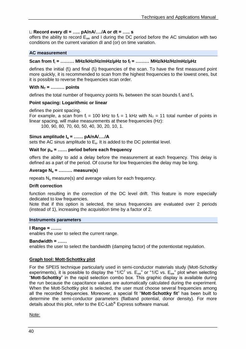
Graph tool: Mott-Schottky plot
For the SPEIS technique particularly used in semi-conductor materials study (Mott-Schottky experiments), it is possible to display the “1/C2 vs. Ewe” or “1/C vs. Ewe” plot when selecting “Mott-Schottky” in the rapid selection combo box. This graphic display is available during the run because the capacitance values are automatically calculated during the experiment. When the Mott-Schottky plot is selected, the user must choose several frequencies among all the recorded frequencies. Moreover, a special fit “Mott-Schottky fit” has been built to determine the semi-conductor parameters (flatband potential, donor density). For more
details about this plot, refer to the EC-Lab Express software manual. Note:
Techniques and Applications Manual
41
Note that potential amplitude (Va) is related to Vpp by Va = Vpp/2 or to the Root Mean
Square (RMS) voltage related to Vpp by VRMS = Vpp/(2 2 ),
it is possible to modify on-line the settings of an impedance measurement during the experiment. To accept the change the user has to click on the Update button
.
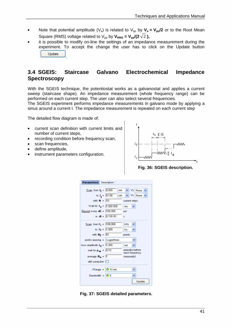
3.4 SGEIS: Staircase Galvano Electrochemical Impedance Spectroscopy
With the SGEIS technique, the potentiostat works as a galvanostat and applies a current sweep (staircase shape). An impedance measurement (whole frequency range) can be performed on each current step. The user can also select several frequencies. The SGEIS experiment performs impedance measurements in galvano mode by applying a sinus around a current I. The impedance measurement is repeated on each current step The detailed flow diagram is made of:
current scan definition with current limits and number of current steps,
recording condition before frequency scan,
scan frequencies,
define amplitude,
instrument parameters configuration.
Fig. 36: SGEIS description.
Fig. 37: SGEIS detailed parameters.
Techniques and Applications Manual
42
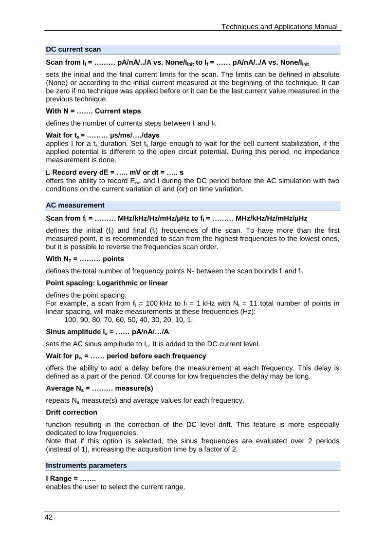
DC current scan
Scan from Ii = ……… pA/nA/../A vs. None/Iinit to If = …… pA/nA/../A vs. None/Iinit
sets the initial and the final current limits for the scan. The limits can be defined in absolute (None) or according to the initial current measured at the beginning of the technique. It can be zero if no technique was applied before or it can be the last current value measured in the previous technique.
With N = ……. Current steps
defines the number of currents steps between Ii and If.
Wait for ts = ……… µs/ms/…./days applies I for a ts duration. Set ts large enough to wait for the cell current stabilization, if the applied potential is different to the open circuit potential. During this period, no impedance measurement is done.
Record every dE = ….. mV or dt = ….. s offers the ability to record Ewe and I during the DC period before the AC simulation with two conditions on the current variation dI and (or) on time variation. AC measurement
Scan from fi = ……… MHz/kHz/Hz/mHz/µHz to ff = ……… MHz/kHz/Hz/mHz/µHz
defines the initial (fi) and final (ff) frequencies of the scan. To have more than the first measured point, it is recommended to scan from the highest frequencies to the lowest ones, but it is possible to reverse the frequencies scan order.
With NT = ……… points
defines the total number of frequency points NT between the scan bounds fi and ff.
Point spacing: Logarithmic or linear
defines the point spacing. For example, a scan from fi = 100 kHz to ff = 1 kHz with Nt = 11 total number of points in linear spacing, will make measurements at these frequencies (Hz): 100, 90, 80, 70, 60, 50, 40, 30, 20, 10, 1.
Sinus amplitude Ia = …… pA/nA/…/A
sets the AC sinus amplitude to Ia. It is added to the DC current level.
Wait for pw = …… period before each frequency
offers the ability to add a delay before the measurement at each frequency. This delay is defined as a part of the period. Of course for low frequencies the delay may be long.
Average Na = ……… measure(s)
repeats Na measure(s) and average values for each frequency.
Drift correction
function resulting in the correction of the DC level drift. This feature is more especially dedicated to low frequencies. Note that if this option is selected, the sinus frequencies are evaluated over 2 periods (instead of 1), increasing the acquisition time by a factor of 2. Instruments parameters
I Range = ……. enables the user to select the current range.

Techniques and Applications Manual
43
Bandwidth = …… enables the user to select the bandwidth (damping factor) of the potentiostat regulation.
Techniques and Applications Manual
44
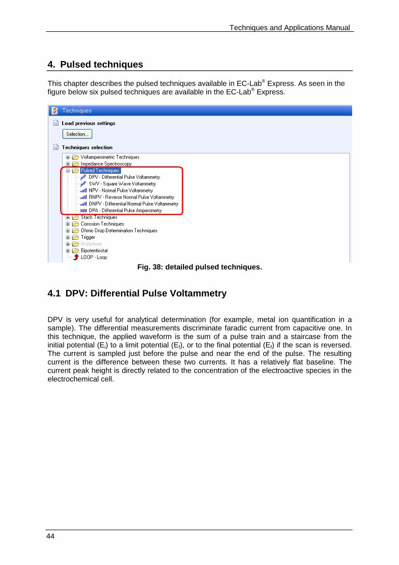
4. Pulsed techniques
This chapter describes the pulsed techniques available in EC-Lab® Express. As seen in the figure below six pulsed techniques are available in the EC-Lab® Express.
Fig. 38: detailed pulsed techniques.
4.1 DPV: Differential Pulse Voltammetry
DPV is very useful for analytical determination (for example, metal ion quantification in a sample). The differential measurements discriminate faradic current from capacitive one. In this technique, the applied waveform is the sum of a pulse train and a staircase from the initial potential (Ei) to a limit potential (Ef), or to the final potential (Ef) if the scan is reversed. The current is sampled just before the pulse and near the end of the pulse. The resulting current is the difference between these two currents. It has a relatively flat baseline. The current peak height is directly related to the concentration of the electroactive species in the electrochemical cell.
Techniques and Applications Manual
45
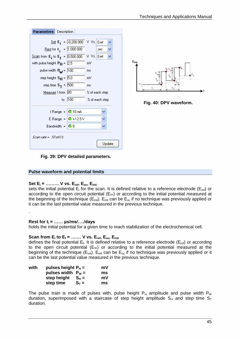
Fig. 39: DPV detailed parameters.
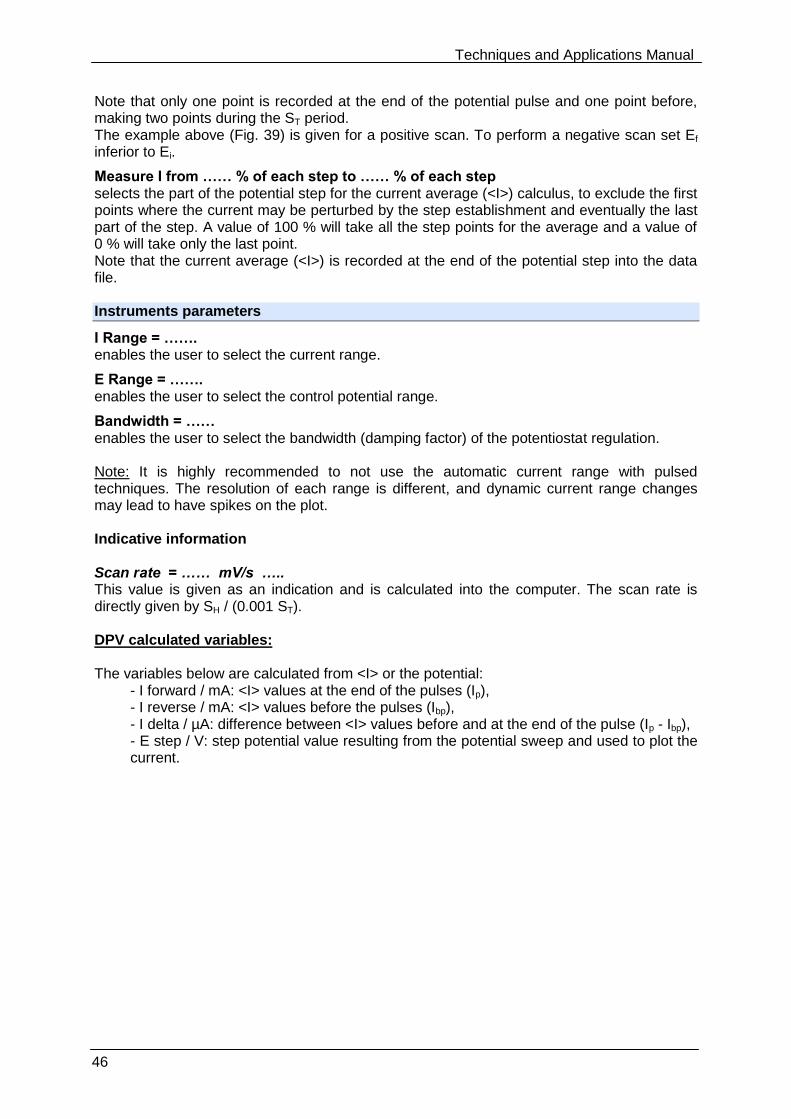
Fig. 40: DPV waveform.
Pulse waveform and potential limits
Set Ei = ……… V vs. Eref, Eoc, Einit sets the initial potential Ei for the scan. It is defined relative to a reference electrode (Eref) or according to the open circuit potential (Eoc) or according to the initial potential measured at the beginning of the technique (Einit). Einit can be Eoc if no technique was previously applied or it can be the last potential value measured in the previous technique.
. Rest for ti = …… µs/ms/…./days holds the initial potential for a given time to reach stabilization of the electrochemical cell. Scan from Ei to Ef = ……. V vs. Eref, Eoc, Einit defines the final potential Ef. It is defined relative to a reference electrode (Eref) or according to the open circuit potential (Eoc) or according to the initial potential measured at the beginning of the technique (Einit). Einit can be Eoc if no technique was previously applied or it can be the last potential value measured in the previous technique. with pulses height PH = mV
pulses width PW = ms step height SH = mV step time ST = ms
The pulse train is made of pulses with, pulse height PH amplitude and pulse width PW duration, superimposed with a staircase of step height amplitude SH and step time ST duration.
Techniques and Applications Manual
46
Note that only one point is recorded at the end of the potential pulse and one point before, making two points during the ST period. The example above (Fig. 39) is given for a positive scan. To perform a negative scan set Ef inferior to Ei.
Measure I from …… % of each step to …… % of each step selects the part of the potential step for the current average (<I>) calculus, to exclude the first points where the current may be perturbed by the step establishment and eventually the last part of the step. A value of 100 % will take all the step points for the average and a value of 0 % will take only the last point. Note that the current average (<I>) is recorded at the end of the potential step into the data file. Instruments parameters
I Range = ……. enables the user to select the current range.
E Range = ……. enables the user to select the control potential range.
Bandwidth = …… enables the user to select the bandwidth (damping factor) of the potentiostat regulation. Note: It is highly recommended to not use the automatic current range with pulsed techniques. The resolution of each range is different, and dynamic current range changes may lead to have spikes on the plot. Indicative information Scan rate = …… mV/s ….. This value is given as an indication and is calculated into the computer. The scan rate is directly given by SH / (0.001 ST). DPV calculated variables: The variables below are calculated from <I> or the potential:
- I forward / mA: <I> values at the end of the pulses (Ip), - I reverse / mA: <I> values before the pulses (Ibp), - I delta / µA: difference between <I> values before and at the end of the pulse (Ip - Ibp), - E step / V: step potential value resulting from the potential sweep and used to plot the current.
Techniques and Applications Manual
47
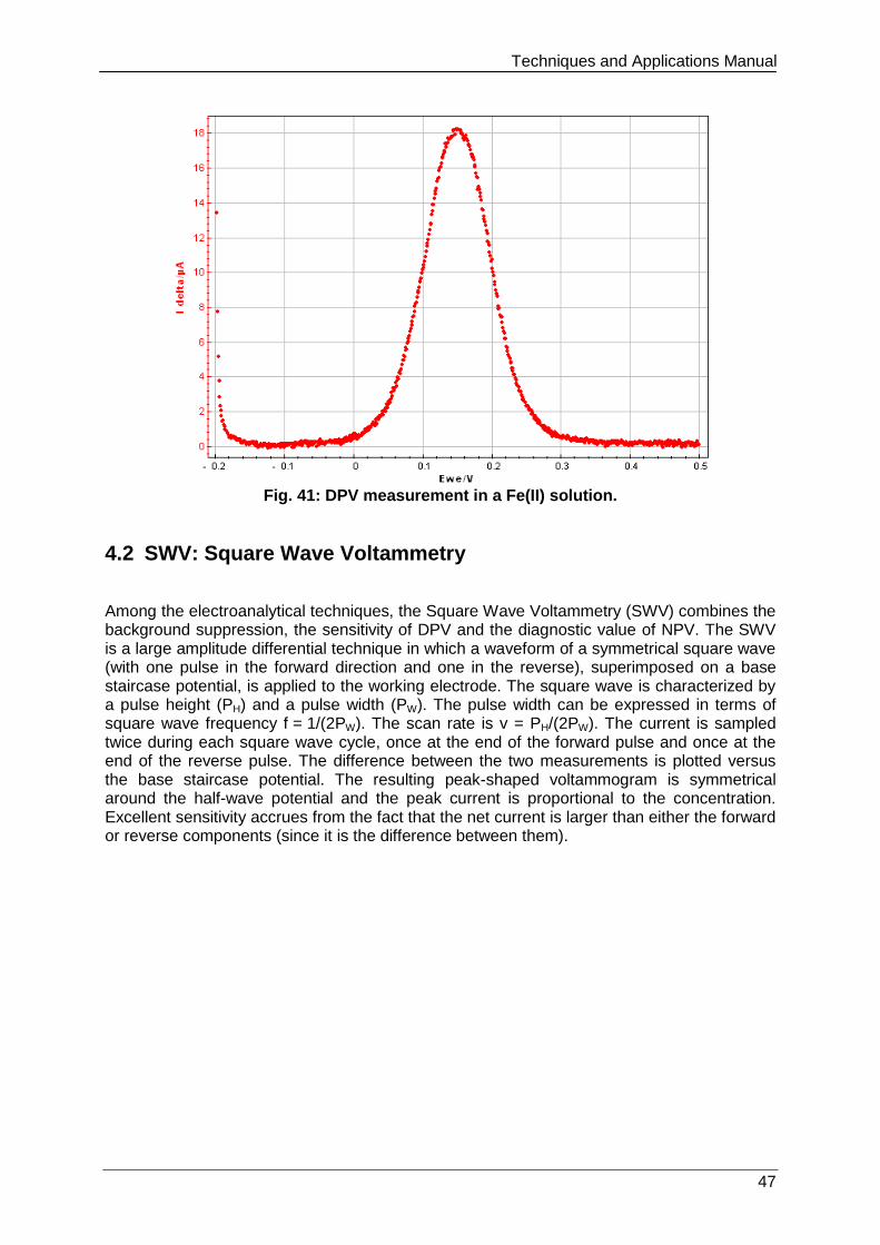
Fig. 41: DPV measurement in a Fe(II) solution.
4.2 SWV: Square Wave Voltammetry
Among the electroanalytical techniques, the Square Wave Voltammetry (SWV) combines the background suppression, the sensitivity of DPV and the diagnostic value of NPV. The SWV is a large amplitude differential technique in which a waveform of a symmetrical square wave (with one pulse in the forward direction and one in the reverse), superimposed on a base staircase potential, is applied to the working electrode. The square wave is characterized by a pulse height (PH) and a pulse width (PW). The pulse width can be expressed in terms of square wave frequency f = 1/(2PW). The scan rate is v = PH/(2PW). The current is sampled twice during each square wave cycle, once at the end of the forward pulse and once at the end of the reverse pulse. The difference between the two measurements is plotted versus the base staircase potential. The resulting peak-shaped voltammogram is symmetrical around the half-wave potential and the peak current is proportional to the concentration. Excellent sensitivity accrues from the fact that the net current is larger than either the forward or reverse components (since it is the difference between them).
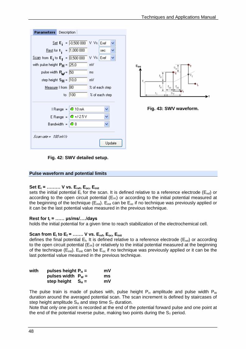
Techniques and Applications Manual
48
Fig. 42: SWV detailed setup.
Fig. 43: SWV waveform.
Pulse waveform and potential limits
Set Ei = ……… V vs. Eref, Eoc, Einit sets the initial potential Ei for the scan. It is defined relative to a reference electrode (Eref) or according to the open circuit potential (Eoc) or according to the initial potential measured at the beginning of the technique (Einit). Einit can be Eoc if no technique was previously applied or it can be the last potential value measured in the previous technique. Rest for ti = …… µs/ms/…./days holds the initial potential for a given time to reach stabilization of the electrochemical cell. Scan from Ei to Ef = ……. V vs. Eref, Eoc, Einit defines the final potential Ef, It is defined relative to a reference electrode (Eref) or according to the open circuit potential (Eoc) or relatively to the initial potential measured at the beginning of the technique (Einit). Einit can be Eoc if no technique was previously applied or it can be the last potential value measured in the previous technique.
with pulses height PH = mV pulses width PW = ms step height SH = mV
The pulse train is made of pulses with, pulse height PH amplitude and pulse width PW duration around the averaged potential scan. The scan increment is defined by staircases of step height amplitude SH and step time ST duration. Note that only one point is recorded at the end of the potential forward pulse and one point at the end of the potential reverse pulse, making two points during the ST period.
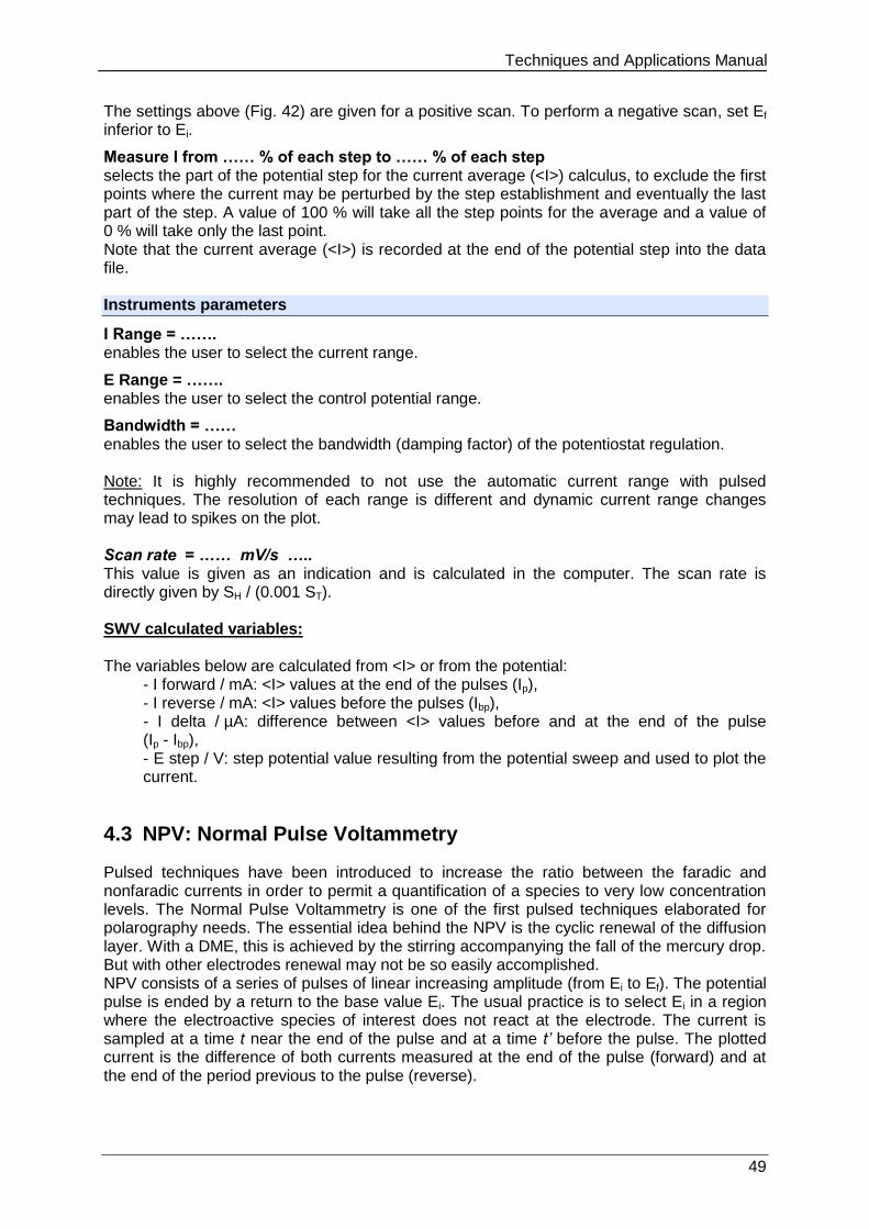
Techniques and Applications Manual
49
The settings above (Fig. 42) are given for a positive scan. To perform a negative scan, set Ef inferior to Ei.
Measure I from …… % of each step to …… % of each step selects the part of the potential step for the current average (<I>) calculus, to exclude the first points where the current may be perturbed by the step establishment and eventually the last part of the step. A value of 100 % will take all the step points for the average and a value of 0 % will take only the last point. Note that the current average (<I>) is recorded at the end of the potential step into the data file. Instruments parameters
I Range = ……. enables the user to select the current range.
E Range = ……. enables the user to select the control potential range.
Bandwidth = …… enables the user to select the bandwidth (damping factor) of the potentiostat regulation. Note: It is highly recommended to not use the automatic current range with pulsed techniques. The resolution of each range is different and dynamic current range changes may lead to spikes on the plot. Scan rate = …… mV/s ….. This value is given as an indication and is calculated in the computer. The scan rate is directly given by SH / (0.001 ST). SWV calculated variables: The variables below are calculated from <I> or from the potential:
- I forward / mA: <I> values at the end of the pulses (Ip), - I reverse / mA: <I> values before the pulses (Ibp), - I delta / µA: difference between <I> values before and at the end of the pulse (Ip - Ibp), - E step / V: step potential value resulting from the potential sweep and used to plot the current.
4.3 NPV: Normal Pulse Voltammetry
Pulsed techniques have been introduced to increase the ratio between the faradic and nonfaradic currents in order to permit a quantification of a species to very low concentration levels. The Normal Pulse Voltammetry is one of the first pulsed techniques elaborated for polarography needs. The essential idea behind the NPV is the cyclic renewal of the diffusion layer. With a DME, this is achieved by the stirring accompanying the fall of the mercury drop. But with other electrodes renewal may not be so easily accomplished. NPV consists of a series of pulses of linear increasing amplitude (from Ei to Ef). The potential pulse is ended by a return to the base value Ei. The usual practice is to select Ei in a region where the electroactive species of interest does not react at the electrode. The current is sampled at a time t near the end of the pulse and at a time t’ before the pulse. The plotted current is the difference of both currents measured at the end of the pulse (forward) and at the end of the period previous to the pulse (reverse).
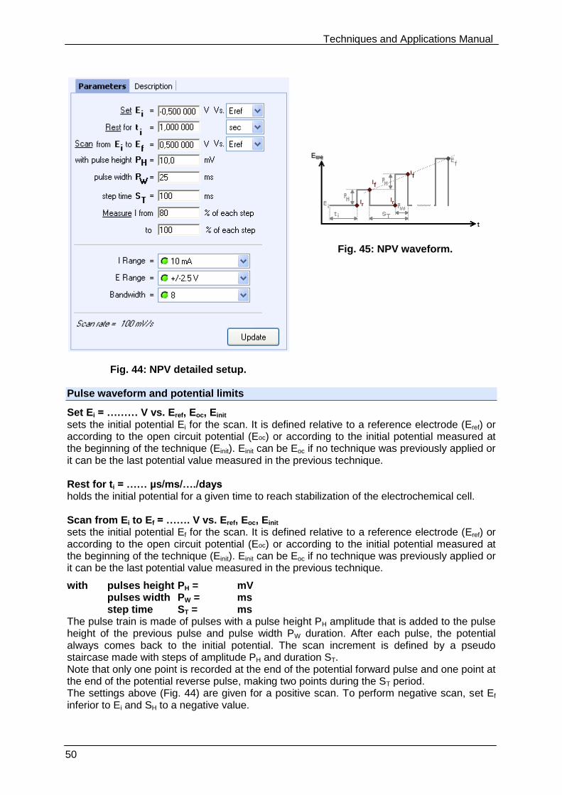
Techniques and Applications Manual
50
Fig. 44: NPV detailed setup.
Fig. 45: NPV waveform.
Pulse waveform and potential limits
Set Ei = ……… V vs. Eref, Eoc, Einit sets the initial potential Ei for the scan. It is defined relative to a reference electrode (Eref) or according to the open circuit potential (Eoc) or according to the initial potential measured at the beginning of the technique (Einit). Einit can be Eoc if no technique was previously applied or it can be the last potential value measured in the previous technique. Rest for ti = …… µs/ms/…./days holds the initial potential for a given time to reach stabilization of the electrochemical cell. Scan from Ei to Ef = ……. V vs. Eref, Eoc, Einit sets the initial potential Ef for the scan. It is defined relative to a reference electrode (Eref) or according to the open circuit potential (Eoc) or according to the initial potential measured at the beginning of the technique (Einit). Einit can be Eoc if no technique was previously applied or it can be the last potential value measured in the previous technique.
with pulses height PH = mV pulses width PW = ms step time ST = ms
The pulse train is made of pulses with a pulse height PH amplitude that is added to the pulse height of the previous pulse and pulse width PW duration. After each pulse, the potential always comes back to the initial potential. The scan increment is defined by a pseudo staircase made with steps of amplitude PH and duration ST. Note that only one point is recorded at the end of the potential forward pulse and one point at the end of the potential reverse pulse, making two points during the ST period. The settings above (Fig. 44) are given for a positive scan. To perform negative scan, set Ef inferior to Ei and SH to a negative value.
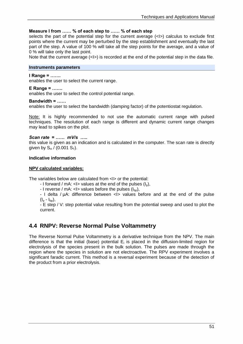
Techniques and Applications Manual
51
Measure I from …… % of each step to …… % of each step selects the part of the potential step for the current average (<I>) calculus to exclude first points where the current may be perturbed by the step establishment and eventually the last part of the step. A value of 100 % will take all the step points for the average, and a value of 0 % will take only the last point. Note that the current average (<I>) is recorded at the end of the potential step in the data file. Instruments parameters
I Range = ……. enables the user to select the current range.
E Range = ……. enables the user to select the control potential range.
Bandwidth = …… enables the user to select the bandwidth (damping factor) of the potentiostat regulation. Note: It is highly recommended to not use the automatic current range with pulsed techniques. The resolution of each range is different and dynamic current range changes may lead to spikes on the plot. Scan rate = …… mV/s ….. this value is given as an indication and is calculated in the computer. The scan rate is directly given by SH / (0.001 ST). Indicative information NPV calculated variables: The variables below are calculated from <I> or the potential:
- I forward / mA: <I> values at the end of the pulses (Ip), - I reverse / mA: <I> values before the pulses (Ibp), - I delta / µA: difference between <I> values before and at the end of the pulse (Ip - Ibp), - E step / V: step potential value resulting from the potential sweep and used to plot the current.
4.4 RNPV: Reverse Normal Pulse Voltammetry
The Reverse Normal Pulse Voltammetry is a derivative technique from the NPV. The main difference is that the initial (base) potential Ei is placed in the diffusion-limited region for electrolysis of the species present in the bulk solution. The pulses are made through the region where the species in solution are not electroactive. The RPV experiment involves a significant faradic current. This method is a reversal experiment because of the detection of the product from a prior electrolysis.
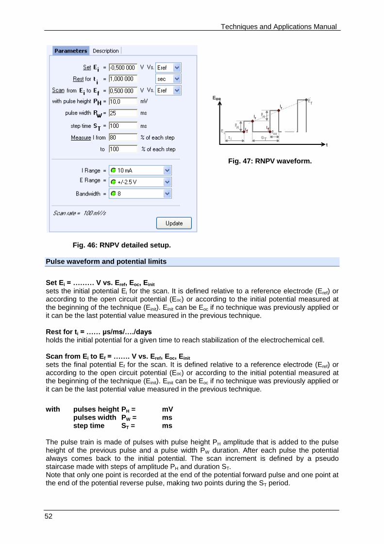
Techniques and Applications Manual
52
Fig. 46: RNPV detailed setup.
Fig. 47: RNPV waveform.
Pulse waveform and potential limits
Set Ei = ……… V vs. Eref, Eoc, Einit sets the initial potential Ei for the scan. It is defined relative to a reference electrode (Eref) or according to the open circuit potential (Eoc) or according to the initial potential measured at the beginning of the technique (Einit). Einit can be Eoc if no technique was previously applied or it can be the last potential value measured in the previous technique. Rest for ti = …… µs/ms/…./days holds the initial potential for a given time to reach stabilization of the electrochemical cell. Scan from Ei to Ef = ……. V vs. Eref, Eoc, Einit sets the final potential Ef for the scan. It is defined relative to a reference electrode (Eref) or according to the open circuit potential (Eoc) or according to the initial potential measured at the beginning of the technique (Einit). Einit can be Eoc if no technique was previously applied or it can be the last potential value measured in the previous technique.
with pulses height PH = mV pulses width PW = ms step time ST = ms
The pulse train is made of pulses with pulse height PH amplitude that is added to the pulse height of the previous pulse and a pulse width PW duration. After each pulse the potential always comes back to the initial potential. The scan increment is defined by a pseudo staircase made with steps of amplitude PH and duration ST. Note that only one point is recorded at the end of the potential forward pulse and one point at the end of the potential reverse pulse, making two points during the ST period.
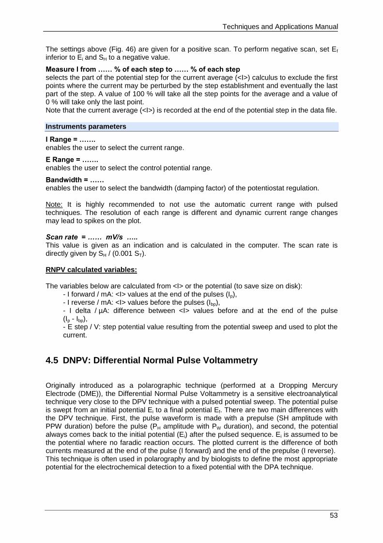
Techniques and Applications Manual
53
The settings above (Fig. 46) are given for a positive scan. To perform negative scan, set Ef inferior to Ei and SH to a negative value.
Measure I from …… % of each step to …… % of each step selects the part of the potential step for the current average (<I>) calculus to exclude the first points where the current may be perturbed by the step establishment and eventually the last part of the step. A value of 100 % will take all the step points for the average and a value of 0 % will take only the last point. Note that the current average (<I>) is recorded at the end of the potential step in the data file. Instruments parameters
I Range = ……. enables the user to select the current range.
E Range = ……. enables the user to select the control potential range.
Bandwidth = …… enables the user to select the bandwidth (damping factor) of the potentiostat regulation. Note: It is highly recommended to not use the automatic current range with pulsed techniques. The resolution of each range is different and dynamic current range changes may lead to spikes on the plot. Scan rate = …… mV/s ….. This value is given as an indication and is calculated in the computer. The scan rate is directly given by SH / (0.001 ST). RNPV calculated variables: The variables below are calculated from <I> or the potential (to save size on disk):
- I forward / mA: <I> values at the end of the pulses (Ip), - I reverse / mA: <I> values before the pulses (Ibp), - I delta / µA: difference between <I> values before and at the end of the pulse (Ip - Ibp), - E step / V: step potential value resulting from the potential sweep and used to plot the current.
4.5 DNPV: Differential Normal Pulse Voltammetry
Originally introduced as a polarographic technique (performed at a Dropping Mercury Electrode (DME)), the Differential Normal Pulse Voltammetry is a sensitive electroanalytical technique very close to the DPV technique with a pulsed potential sweep. The potential pulse is swept from an initial potential Ei to a final potential Ef. There are two main differences with the DPV technique. First, the pulse waveform is made with a prepulse (SH amplitude with PPW duration) before the pulse (PH amplitude with PW duration), and second, the potential always comes back to the initial potential (Ei) after the pulsed sequence. Ei is assumed to be the potential where no faradic reaction occurs. The plotted current is the difference of both currents measured at the end of the pulse (I forward) and the end of the prepulse (I reverse). This technique is often used in polarography and by biologists to define the most appropriate potential for the electrochemical detection to a fixed potential with the DPA technique.
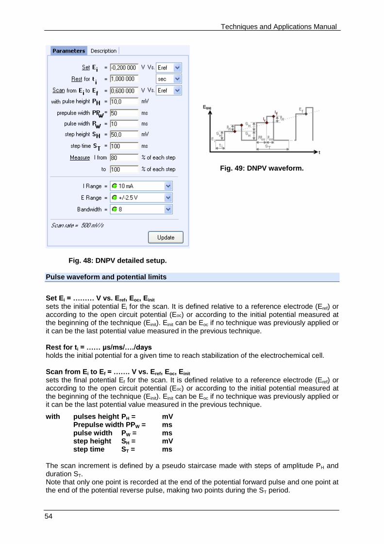
Techniques and Applications Manual
54
Fig. 48: DNPV detailed setup.
Fig. 49: DNPV waveform.
Pulse waveform and potential limits
Set Ei = ……… V vs. Eref, Eoc, Einit sets the initial potential Ei for the scan. It is defined relative to a reference electrode (Eref) or according to the open circuit potential (Eoc) or according to the initial potential measured at the beginning of the technique (Einit). Einit can be Eoc if no technique was previously applied or it can be the last potential value measured in the previous technique. Rest for ti = …… µs/ms/…./days holds the initial potential for a given time to reach stabilization of the electrochemical cell. Scan from Ei to Ef = ……. V vs. Eref, Eoc, Einit sets the final potential Ef for the scan. It is defined relative to a reference electrode (Eref) or according to the open circuit potential (Eoc) or according to the initial potential measured at the beginning of the technique (Einit). Einit can be Eoc if no technique was previously applied or it can be the last potential value measured in the previous technique.
with pulses height PH = mV Prepulse width PPW = ms
pulse width PW = ms step height SH = mV step time ST = ms
The scan increment is defined by a pseudo staircase made with steps of amplitude PH and duration ST. Note that only one point is recorded at the end of the potential forward pulse and one point at the end of the potential reverse pulse, making two points during the ST period.
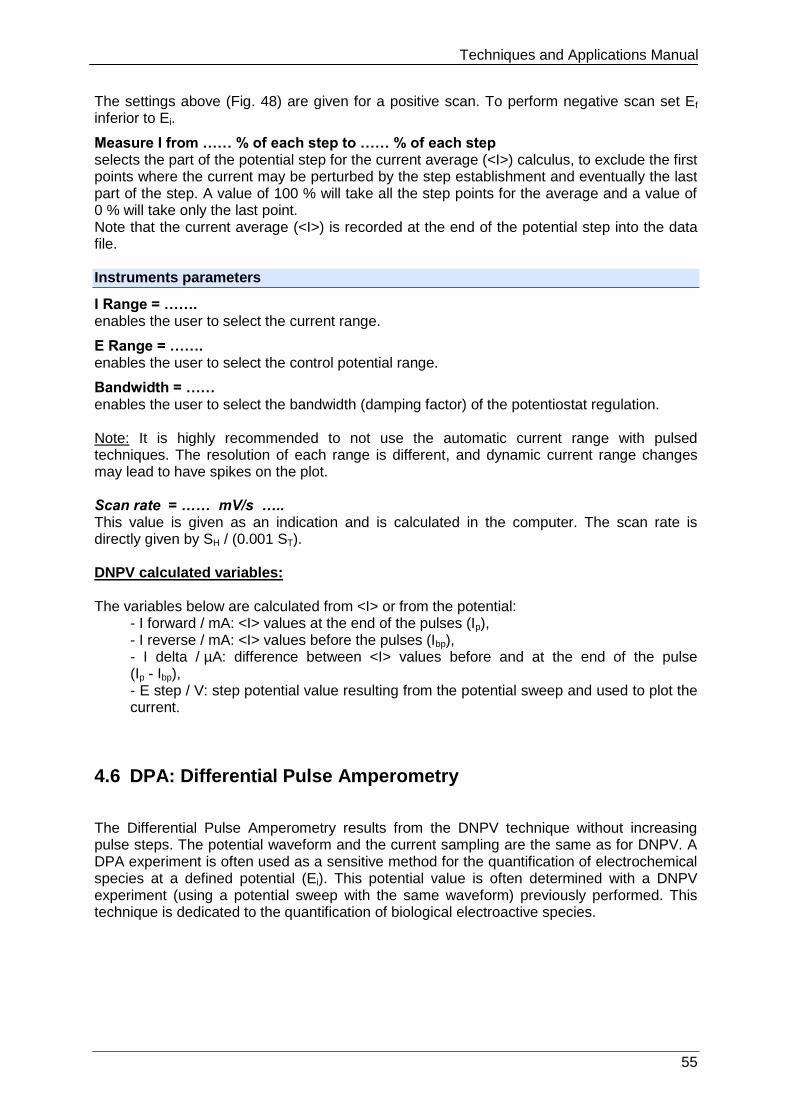
Techniques and Applications Manual
55
The settings above (Fig. 48) are given for a positive scan. To perform negative scan set Ef inferior to Ei.
Measure I from …… % of each step to …… % of each step selects the part of the potential step for the current average (<I>) calculus, to exclude the first points where the current may be perturbed by the step establishment and eventually the last part of the step. A value of 100 % will take all the step points for the average and a value of 0 % will take only the last point. Note that the current average (<I>) is recorded at the end of the potential step into the data file. Instruments parameters
I Range = ……. enables the user to select the current range.
E Range = ……. enables the user to select the control potential range.
Bandwidth = …… enables the user to select the bandwidth (damping factor) of the potentiostat regulation. Note: It is highly recommended to not use the automatic current range with pulsed techniques. The resolution of each range is different, and dynamic current range changes may lead to have spikes on the plot. Scan rate = …… mV/s ….. This value is given as an indication and is calculated in the computer. The scan rate is directly given by SH / (0.001 ST). DNPV calculated variables: The variables below are calculated from <I> or from the potential:
- I forward / mA: <I> values at the end of the pulses (Ip), - I reverse / mA: <I> values before the pulses (Ibp), - I delta / µA: difference between <I> values before and at the end of the pulse (Ip - Ibp), - E step / V: step potential value resulting from the potential sweep and used to plot the current.
4.6 DPA: Differential Pulse Amperometry
The Differential Pulse Amperometry results from the DNPV technique without increasing pulse steps. The potential waveform and the current sampling are the same as for DNPV. A DPA experiment is often used as a sensitive method for the quantification of electrochemical species at a defined potential (Ei). This potential value is often determined with a DNPV experiment (using a potential sweep with the same waveform) previously performed. This technique is dedicated to the quantification of biological electroactive species.
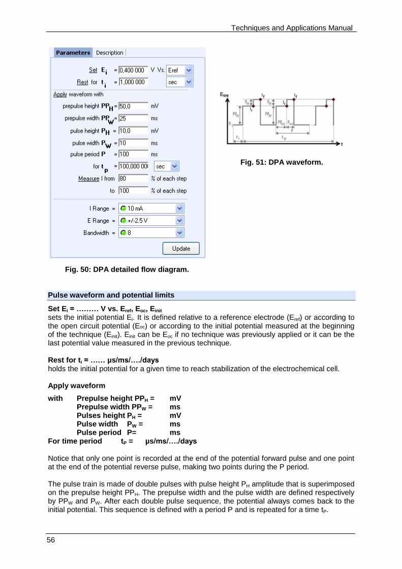
Techniques and Applications Manual
56
Fig. 50: DPA detailed flow diagram.
Fig. 51: DPA waveform.
Pulse waveform and potential limits
Set Ei = ……… V vs. Eref, Eoc, Einit sets the initial potential Ei. It is defined relative to a reference electrode (Eref) or according to the open circuit potential (Eoc) or according to the initial potential measured at the beginning of the technique (Einit). Einit can be Eoc if no technique was previously applied or it can be the last potential value measured in the previous technique. Rest for ti = …… µs/ms/…./days holds the initial potential for a given time to reach stabilization of the electrochemical cell. Apply waveform
with Prepulse height PPH = mV Prepulse width PPW = ms Pulses height PH = mV
Pulse width PW = ms Pulse period P= ms
For time period tP = µs/ms/…./days
Notice that only one point is recorded at the end of the potential forward pulse and one point at the end of the potential reverse pulse, making two points during the P period. The pulse train is made of double pulses with pulse height PH amplitude that is superimposed on the prepulse height PPH. The prepulse width and the pulse width are defined respectively by PPW and PW. After each double pulse sequence, the potential always comes back to the initial potential. This sequence is defined with a period P and is repeated for a time tP.
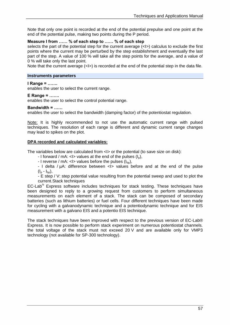
Techniques and Applications Manual
57
Note that only one point is recorded at the end of the potential prepulse and one point at the end of the potential pulse, making two points during the P period.
Measure I from …… % of each step to …… % of each step selects the part of the potential step for the current average (<I>) calculus to exclude the first points where the current may be perturbed by the step establishment and eventually the last part of the step. A value of 100 % will take all the step points for the average, and a value of 0 % will take only the last point. Note that the current average (<I>) is recorded at the end of the potential step in the data file. Instruments parameters
I Range = ……. enables the user to select the current range.
E Range = ……. enables the user to select the control potential range.
Bandwidth = …… enables the user to select the bandwidth (damping factor) of the potentiostat regulation. Note: It is highly recommended to not use the automatic current range with pulsed techniques. The resolution of each range is different and dynamic current range changes may lead to spikes on the plot. DPA recorded and calculated variables: The variables below are calculated from <I> or the potential (to save size on disk):
- I forward / mA: <I> values at the end of the pulses (Ip), - I reverse / mA: <I> values before the pulses (Ibp), - I delta / µA: difference between <I> values before and at the end of the pulse (Ip - Ibp), - E step / V: step potential value resulting from the potential sweep and used to plot the current.Stack techniques
EC-Lab Express software includes techniques for stack testing. These techniques have been designed to reply to a growing request from customers to perform simultaneous measurements on each element of a stack. The stack can be composed of secondary batteries (such as lithium batteries) or fuel cells. Four different techniques have been made for cycling with a galvanodynamic technique and a potentiodynamic technique and for EIS measurement with a galvano EIS and a potentio EIS technique. The stack techniques have been improved with respect to the previous version of EC-Lab® Express. It is now possible to perform stack experiment on numerous potentiostat channels. the total voltage of the stack must not exceed 20 V and are available only for VMP3 technology (not available for SP-300 technology).
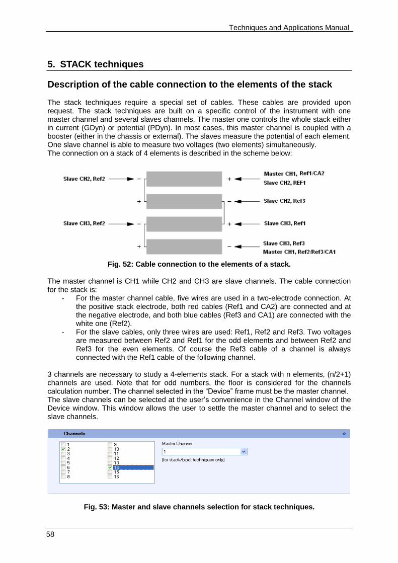
Techniques and Applications Manual
58
5. STACK techniques
Description of the cable connection to the elements of the stack The stack techniques require a special set of cables. These cables are provided upon request. The stack techniques are built on a specific control of the instrument with one master channel and several slaves channels. The master one controls the whole stack either in current (GDyn) or potential (PDyn). In most cases, this master channel is coupled with a booster (either in the chassis or external). The slaves measure the potential of each element. One slave channel is able to measure two voltages (two elements) simultaneously. The connection on a stack of 4 elements is described in the scheme below:
Fig. 52: Cable connection to the elements of a stack.
The master channel is CH1 while CH2 and CH3 are slave channels. The cable connection for the stack is:
- For the master channel cable, five wires are used in a two-electrode connection. At the positive stack electrode, both red cables (Ref1 and CA2) are connected and at the negative electrode, and both blue cables (Ref3 and CA1) are connected with the white one (Ref2).
- For the slave cables, only three wires are used: Ref1, Ref2 and Ref3. Two voltages are measured between Ref2 and Ref1 for the odd elements and between Ref2 and Ref3 for the even elements. Of course the Ref3 cable of a channel is always connected with the Ref1 cable of the following channel.
3 channels are necessary to study a 4-elements stack. For a stack with n elements, (n/2+1) channels are used. Note that for odd numbers, the floor is considered for the channels calculation number. The channel selected in the “Device” frame must be the master channel. The slave channels can be selected at the user’s convenience in the Channel window of the Device window. This window allows the user to settle the master channel and to select the slave channels.
Fig. 53: Master and slave channels selection for stack techniques.
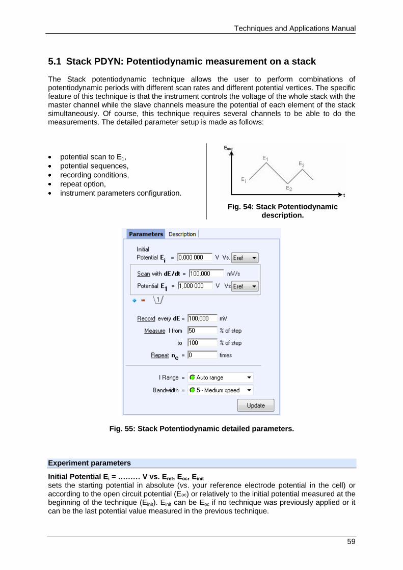
Techniques and Applications Manual
59
5.1 Stack PDYN: Potentiodynamic measurement on a stack
The Stack potentiodynamic technique allows the user to perform combinations of potentiodynamic periods with different scan rates and different potential vertices. The specific feature of this technique is that the instrument controls the voltage of the whole stack with the master channel while the slave channels measure the potential of each element of the stack simultaneously. Of course, this technique requires several channels to be able to do the measurements. The detailed parameter setup is made as follows:
potential scan to E1,
potential sequences,
recording conditions,
repeat option,
instrument parameters configuration.
Fig. 54: Stack Potentiodynamic description.
Fig. 55: Stack Potentiodynamic detailed parameters.
Experiment parameters
Initial Potential Ei = ……… V vs. Eref, Eoc, Einit sets the starting potential in absolute (vs. your reference electrode potential in the cell) or according to the open circuit potential (Eoc) or relatively to the initial potential measured at the beginning of the technique (Einit). Einit can be Eoc if no technique was previously applied or it can be the last potential value measured in the previous technique.
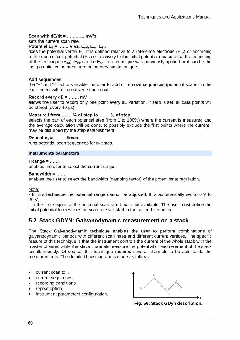
Techniques and Applications Manual
60
Scan with dE/dt = ………… mV/s sets the current scan rate. Potential E1 = ……. V vs. Eref, Eoc, Einit fixes the potential vertex E1. It is defined relative to a reference electrode (Eref) or according to the open circuit potential (Eoc) or relatively to the initial potential measured at the beginning of the technique (Einit). Einit can be Eoc if no technique was previously applied or it can be the last potential value measured in the previous technique.
Add sequences the “+” and “-“ buttons enable the user to add or remove sequences (potential scans) to the experiment with different vertex potential.
Record every dE = ……. mV allows the user to record only one point every dE variation. If zero is set, all data points will be stored (every 40 µs).
Measure I from ……. % of step to ……. % of step selects the part of each potential step (from 1 to 100%) where the current is measured and the average calculation will be done, to possibly exclude the first points where the current l may be disturbed by the step establishment.
Repeat nc = …….. times runs potential scan sequences for nc times. Instruments parameters
I Range = ……. enables the user to select the current range.
Bandwidth = …… enables the user to select the bandwidth (damping factor) of the potentiostat regulation. Note: - In this technique the potential range cannot be adjusted. It is automatically set to 0 V to 20 V, - in the first sequence the potential scan rate box is not available. The user must define the initial potential from where the scan rate will start in the second sequence.
5.2 Stack GDYN: Galvanodynamic measurement on a stack
The Stack Galvanodynamic technique enables the user to perform combinations of galvanodynamic periods with different scan rates and different current vertices. The specific feature of this technique is that the instrument controls the current of the whole stack with the master channel while the slave channels measure the potential of each element of the stack simultaneously. Of course, this technique requires several channels to be able to do the measurements. The detailed flow diagram is made as follows:
current scan to I1,
current sequences,
recording conditions,
repeat option,
instrument parameters configuration.
Fig. 56: Stack GDyn description.
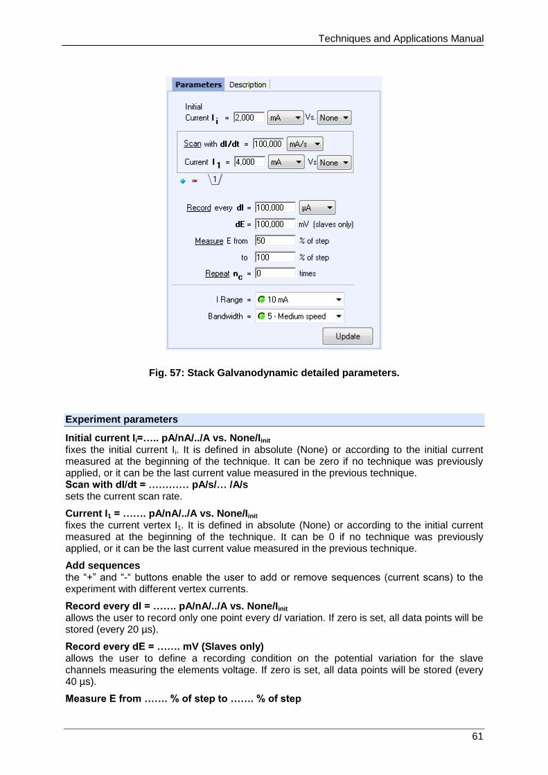
Techniques and Applications Manual
61
Fig. 57: Stack Galvanodynamic detailed parameters.
Experiment parameters
Initial current Ii=….. pA/nA/../A vs. None/Iinit fixes the initial current Ii. It is defined in absolute (None) or according to the initial current measured at the beginning of the technique. It can be zero if no technique was previously applied, or it can be the last current value measured in the previous technique. Scan with dI/dt = ………… pA/s/… /A/s sets the current scan rate.
Current I1 = ……. pA/nA/../A vs. None/Iinit fixes the current vertex I1. It is defined in absolute (None) or according to the initial current measured at the beginning of the technique. It can be 0 if no technique was previously applied, or it can be the last current value measured in the previous technique.
Add sequences the “+” and “-“ buttons enable the user to add or remove sequences (current scans) to the experiment with different vertex currents.
Record every dI = ……. pA/nA/../A vs. None/Iinit allows the user to record only one point every dI variation. If zero is set, all data points will be stored (every 20 µs).
Record every dE = ……. mV (Slaves only) allows the user to define a recording condition on the potential variation for the slave channels measuring the elements voltage. If zero is set, all data points will be stored (every 40 µs).
Measure E from ……. % of step to ……. % of step
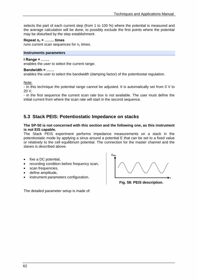
Techniques and Applications Manual
62
selects the part of each current step (from 1 to 100 %) where the potential is measured and the average calculation will be done, to possibly exclude the first points where the potential may be disturbed by the step establishment.
Repeat nc = …….. times runs current scan sequences for nc times. Instruments parameters
I Range = ……. enables the user to select the current range.
Bandwidth = …… enables the user to select the bandwidth (damping factor) of the potentiostat regulation. Note: - In this technique the potential range cannot be adjusted. It is automatically set from 0 V to 20 V, - in the first sequence the current scan rate box is not available. The user must define the initial current from where the scan rate will start in the second sequence.
5.3 Stack PEIS: Potentiostatic Impedance on stacks
The SP-50 is not concerned with this section and the following one, as this instrument is not EIS capable. The Stack PEIS experiment performs impedance measurements on a stack in the potentiostatic mode by applying a sinus around a potential E that can be set to a fixed value or relatively to the cell equilibrium potential. The connection for the master channel and the slaves is described above.
fixe a DC potential,
recording condition before frequency scan,
scan frequencies,
define amplitude,
instrument parameters configuration.
Fig. 58: PEIS description.
The detailed parameter setup is made of:
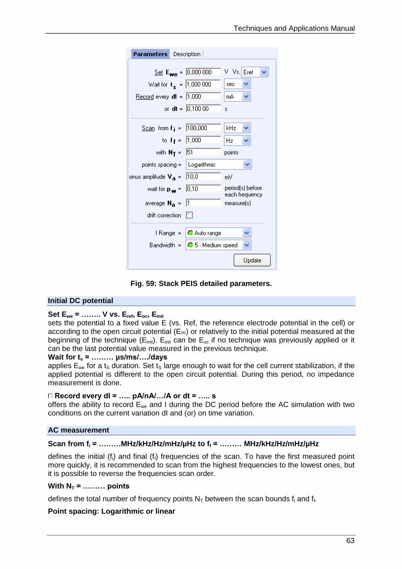
Techniques and Applications Manual
63
Fig. 59: Stack PEIS detailed parameters. Initial DC potential
Set Ewe = …….. V vs. Eref, Eoc, Einit sets the potential to a fixed value E (vs. Ref, the reference electrode potential in the cell) or according to the open circuit potential (Eoc) or relatively to the initial potential measured at the beginning of the technique (Einit). Einit can be Eoc if no technique was previously applied or it can be the last potential value measured in the previous technique. Wait for ts = ……… µs/ms/…./days applies Ewe for a tS duration. Set tS large enough to wait for the cell current stabilization, if the applied potential is different to the open circuit potential. During this period, no impedance measurement is done.
Record every dI = ….. pA/nA/…/A or dt = ….. s offers the ability to record Ewe and I during the DC period before the AC simulation with two conditions on the current variation dI and (or) on time variation. AC measurement
Scan from fi = ………MHz/kHz/Hz/mHz/µHz to ff = ……… MHz/kHz/Hz/mHz/µHz
defines the initial (fi) and final (ff) frequencies of the scan. To have the first measured point more quickly, it is recommended to scan from the highest frequencies to the lowest ones, but it is possible to reverse the frequencies scan order.
With NT = ……… points
defines the total number of frequency points NT between the scan bounds fi and ff.
Point spacing: Logarithmic or linear
Techniques and Applications Manual
64
defines the point spacing. For example, a scan from fi = 100 kHz to ff = 1 kHz with Nt = 11 total number of points in linear spacing will make measurements at these frequencies (Hz): 100, 90, 80, 70, 60, 50, 40, 30, 20, 10, 1.
Sinus amplitude Va = …… V
sets the AC sinus amplitude to Va. It is added to the DC potential level.
Wait for pw = …… period before each frequency
offers the ability to add a delay before the measurement at each frequency. This delay is defined as a part of the period. Of course for low frequencies, the delay may be long.
Average Na = ……… mesure(s)
repeats Na measure(s) and average values for each frequency.
Drift correction function resulting in the correction of the DC level drift. This feature is more especially dedicated to low frequencies. Note that if this option is selected, sinus frequencies are evaluated over 2 periods (instead of 1), increasing the acquisition time by a factor of 2. Instruments parameters
I Range = ……. enables the user to select the current range.
Bandwidth = …… enables the user to select the bandwidth (damping factor) of the potentiostat regulation. Note: In this technique the potential range cannot be adjusted. It is automatically set to 0 V to 20 V.
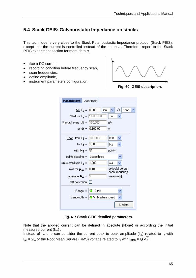
Techniques and Applications Manual
65
5.4 Stack GEIS: Galvanostatic Impedance on stacks
This technique is very close to the Stack Potentiostastic Impedance protocol (Stack PEIS), except that the current is controlled instead of the potential. Therefore, report to the Stack PEIS experiment section for more details.
fixe a DC current,
recording condition before frequency scan,
scan frequencies,
define amplitude,
instrument parameters configuration.
Fig. 60: GEIS description.
Fig. 61: Stack GEIS detailed parameters. Note that the applied current can be defined in absolute (None) or according the initial measured current (Iinit) . Instead of Ia, one can consider the current peak to peak amplitude (Ipp) related to Ia with
Ipp = 2Ia or the Root Mean Square (RMS) voltage related to Ia with IRMS = Ia/ 2 .
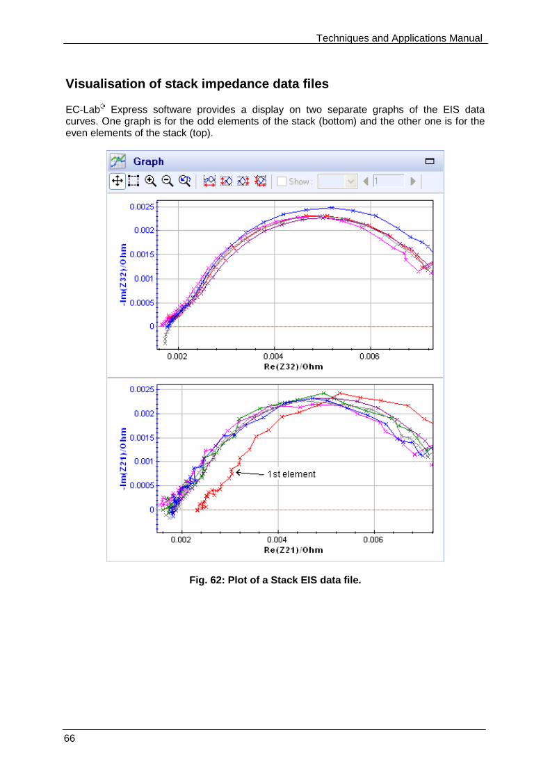
Techniques and Applications Manual
66
Visualisation of stack impedance data files
EC-Lab Express software provides a display on two separate graphs of the EIS data curves. One graph is for the odd elements of the stack (bottom) and the other one is for the even elements of the stack (top).
Fig. 62: Plot of a Stack EIS data file.
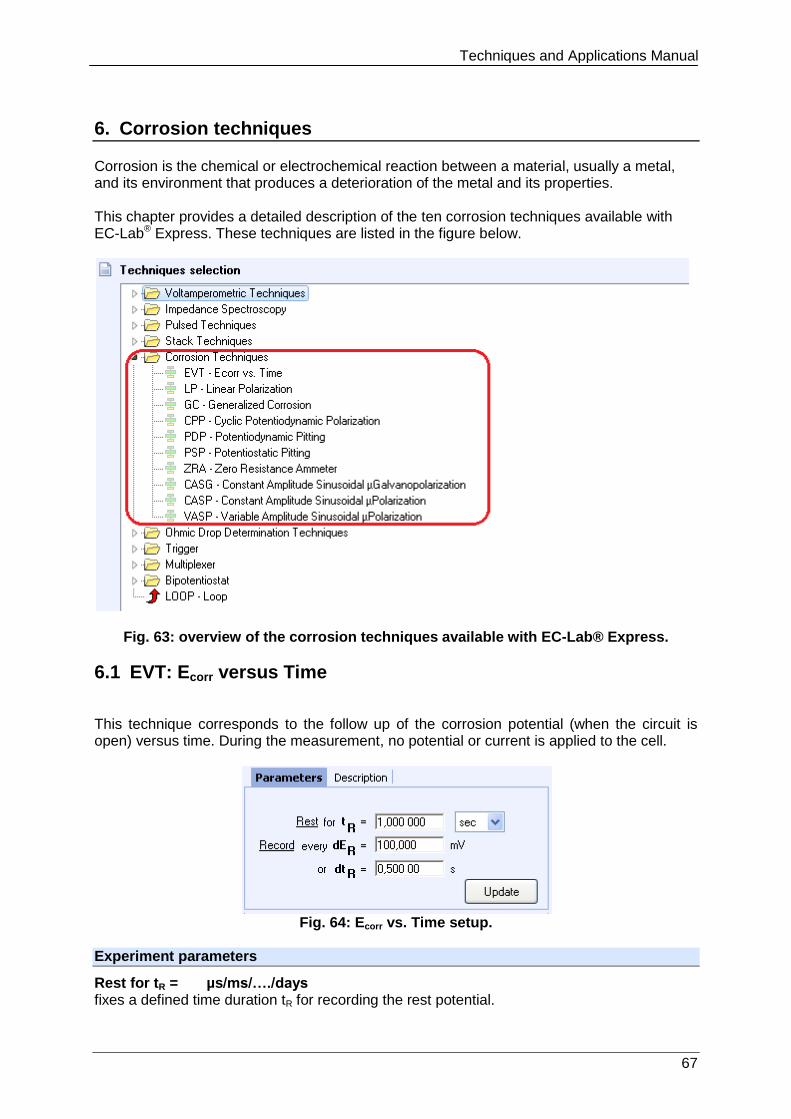
Techniques and Applications Manual
67
6. Corrosion techniques
Corrosion is the chemical or electrochemical reaction between a material, usually a metal, and its environment that produces a deterioration of the metal and its properties. This chapter provides a detailed description of the ten corrosion techniques available with EC-Lab® Express. These techniques are listed in the figure below.
Fig. 63: overview of the corrosion techniques available with EC-Lab® Express.
6.1 EVT: Ecorr versus Time
This technique corresponds to the follow up of the corrosion potential (when the circuit is open) versus time. During the measurement, no potential or current is applied to the cell.
Fig. 64: Ecorr vs. Time setup.
Experiment parameters
Rest for tR = µs/ms/…./days fixes a defined time duration tR for recording the rest potential.
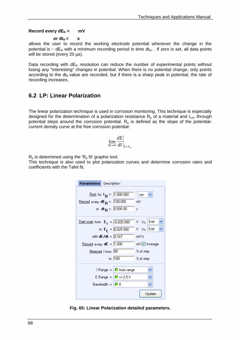
Techniques and Applications Manual
68
Record every dER = mV
or dtR = s allows the user to record the working electrode potential whenever the change in the
potential is dER with a minimum recording period in time dtR. . If zero is set, all data points will be stored (every 20 µs). Data recording with dER resolution can reduce the number of experimental points without losing any "interesting" changes in potential. When there is no potential change, only points according to the dtR value are recorded, but if there is a sharp peak in potential, the rate of recording increases.
6.2 LP: Linear Polarization
The linear polarization technique is used in corrosion monitoring. This technique is especially designed for the determination of a polarization resistance Rp of a material and Icorr through potential steps around the corrosion potential. Rp is defined as the slope of the potential-current density curve at the free corrosion potential:
ocEEdl
dElim
0dE
Rp is determined using the 'Rp fit' graphic tool. This technique is also used to plot polarization curves and determine corrosion rates and coefficients with the Tafel fit.
Fig. 65: Linear Polarization detailed parameters.
Techniques and Applications Manual
69
Open circuit parameters
Rest for tR = µs/ms/…./days fixes a defined time duration tR for recording the rest potential.
Record every dER = mV
or dtR = s allows the user to record the working electrode potential whenever the change in the
potential is dER with a minimum recording period in time dtR.
Scan parameters
Start scan from Ei = …….. V vs. Eref, Eoc, Einit sets the initial potential Ei for the scan. It is defined relative to a reference electrode (Eref) or according to the open circuit potential (Eoc) or according to the initial potential measured at the beginning of the technique (Einit). Einit can be Eoc if no technique was previously applied or it can be the last potential value measured in the previous technique. To EL = …….. V vs. Eref, Eoc, Einit sets the final potential Ef. It is defined relative to a reference electrode (Eref) or according to the open circuit potential (Eoc) or according to the initial potential measured at the beginning of the technique (Einit). Einit can be Eoc if no technique was previously applied or it can be the last potential value measured in the previous technique. With dE/dt = ……. mV/s allows the user to set the scan rate in mV/s The potential step height and its duration are optimized by the software in order to be as close as possible as an analogic scan.
Record every dE = ……. mV allows the user to record only one point every dE variation. If zero is set, all data points will be stored (every 40 µs).
Measure I from ……. % of step to ……. % of step selects the part of each potential step (from 1 to 100%) where the current is measured and the average calculation will be done to possibly exclude the first points where the current may be disturbed by the step establishment. Instruments parameters
I Range = ……. enables the user to select the current range
E Range = ……. enables the user to select the control potential range
Bandwidth = …… enables the user to select the bandwidth (damping factor) of the potentiostat regulation. Related fits to LP
The LP application can be used for Rp and Icorr determination using the Rp fit (see the ECLab Express software manual for more details). It can also be used to determine the corrosion
rate with the Tafel fit (see the EC-Lab Express software manual for more details).
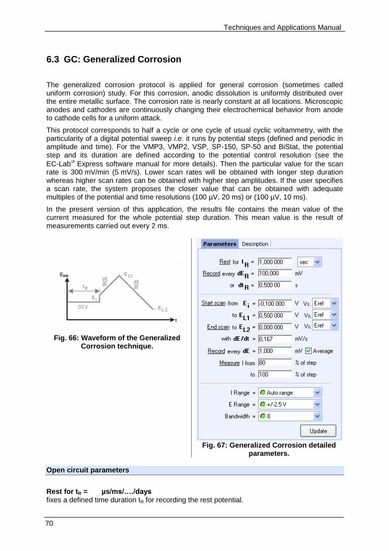
Techniques and Applications Manual
70
6.3 GC: Generalized Corrosion
The generalized corrosion protocol is applied for general corrosion (sometimes called uniform corrosion) study. For this corrosion, anodic dissolution is uniformly distributed over the entire metallic surface. The corrosion rate is nearly constant at all locations. Microscopic anodes and cathodes are continuously changing their electrochemical behavior from anode to cathode cells for a uniform attack.
This protocol corresponds to half a cycle or one cycle of usual cyclic voltammetry, with the particularity of a digital potential sweep i.e. it runs by potential steps (defined and periodic in amplitude and time). For the VMP3, VMP2, VSP, SP-150, SP-50 and BiStat, the potential step and its duration are defined according to the potential control resolution (see the
EC-Lab Express software manual for more details). Then the particular value for the scan rate is 300 mV/min (5 mV/s). Lower scan rates will be obtained with longer step duration whereas higher scan rates can be obtained with higher step amplitudes. If the user specifies a scan rate, the system proposes the closer value that can be obtained with adequate multiples of the potential and time resolutions (100 µV, 20 ms) or (100 µV, 10 ms).
In the present version of this application, the results file contains the mean value of the current measured for the whole potential step duration. This mean value is the result of measurements carried out every 2 ms.
Fig. 66: Waveform of the Generalized Corrosion technique.
Fig. 67: Generalized Corrosion detailed
parameters. Open circuit parameters
Rest for tR = µs/ms/…./days fixes a defined time duration tR for recording the rest potential.
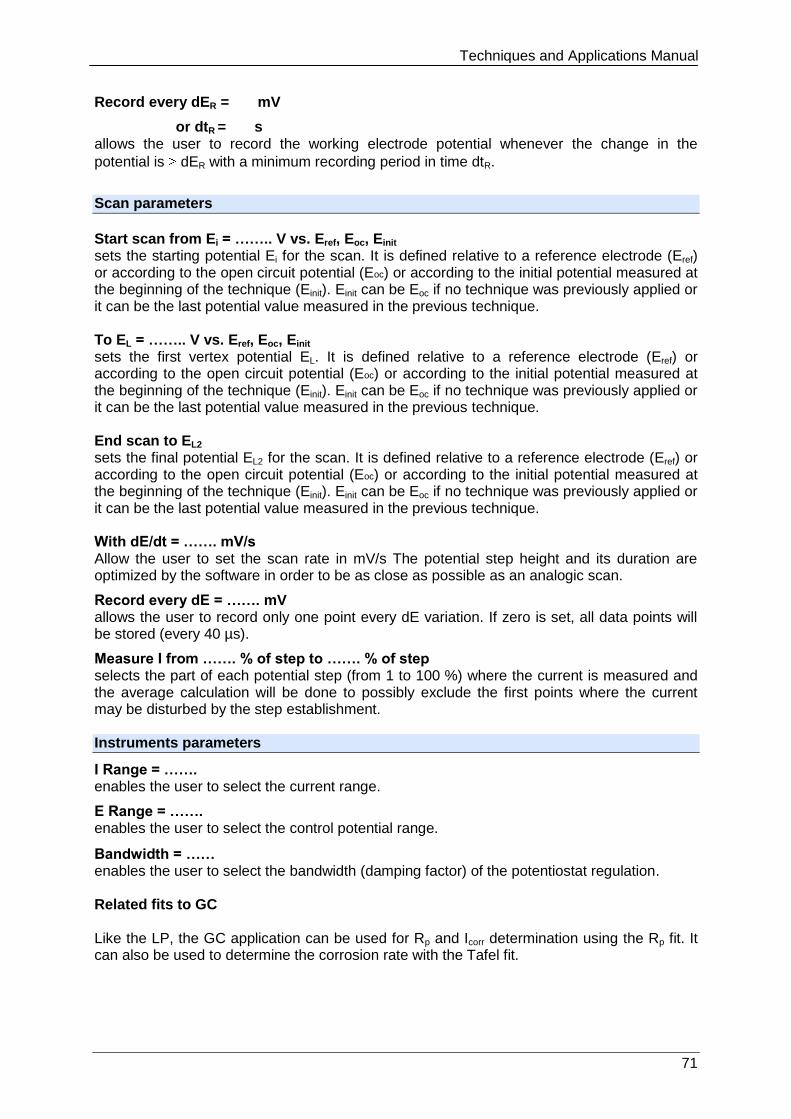
Techniques and Applications Manual
71
Record every dER = mV
or dtR = s allows the user to record the working electrode potential whenever the change in the
potential is dER with a minimum recording period in time dtR.
Scan parameters
Start scan from Ei = …….. V vs. Eref, Eoc, Einit sets the starting potential Ei for the scan. It is defined relative to a reference electrode (Eref) or according to the open circuit potential (Eoc) or according to the initial potential measured at the beginning of the technique (Einit). Einit can be Eoc if no technique was previously applied or it can be the last potential value measured in the previous technique. To EL = …….. V vs. Eref, Eoc, Einit sets the first vertex potential EL. It is defined relative to a reference electrode (Eref) or according to the open circuit potential (Eoc) or according to the initial potential measured at the beginning of the technique (Einit). Einit can be Eoc if no technique was previously applied or it can be the last potential value measured in the previous technique. End scan to EL2 sets the final potential EL2 for the scan. It is defined relative to a reference electrode (Eref) or according to the open circuit potential (Eoc) or according to the initial potential measured at the beginning of the technique (Einit). Einit can be Eoc if no technique was previously applied or it can be the last potential value measured in the previous technique. With dE/dt = ……. mV/s Allow the user to set the scan rate in mV/s The potential step height and its duration are optimized by the software in order to be as close as possible as an analogic scan.
Record every dE = ……. mV allows the user to record only one point every dE variation. If zero is set, all data points will be stored (every 40 µs).
Measure I from ……. % of step to ……. % of step selects the part of each potential step (from 1 to 100 %) where the current is measured and the average calculation will be done to possibly exclude the first points where the current may be disturbed by the step establishment. Instruments parameters
I Range = ……. enables the user to select the current range.
E Range = ……. enables the user to select the control potential range.
Bandwidth = …… enables the user to select the bandwidth (damping factor) of the potentiostat regulation. Related fits to GC Like the LP, the GC application can be used for Rp and Icorr determination using the Rp fit. It can also be used to determine the corrosion rate with the Tafel fit.
Techniques and Applications Manual
72
6.4 CPP: Cyclic Potentiodynamic Polarization
The Cyclic Potentiodynamic Polarization is often used to evaluate pitting susceptibility. It is the most common electrochemical test for localized corrosion resistance. The potential is swept in a single cycle or slightly less than one cycle. The size of the hysteresis is examined along with the difference between the values of the starting open circuit corrosion potential and the return passivation potential. The existence of hysteresis is usually indicative of pitting, while the size of the loop is often related to the amount of pitting. This application is based both on the MPP and MPSP protocols, except that the potentiodynamic phase is done before the potentiostatic one, some phases are optional and there is an additional potentiodynamic phase:
Fig. 68: CPP potential waveform.
The detailed setup is made of:
initial rest potential sequence,
potential sweep with threshold pitting detection,
hold potential,
reverse scan.
Fig. 69: CPP detailed parameters. Open circuit parameters
Rest for tR = µs/ms/…./days fixes a defined time duration tR for recording the rest potential.
Record every dER = mV
or dtR = s
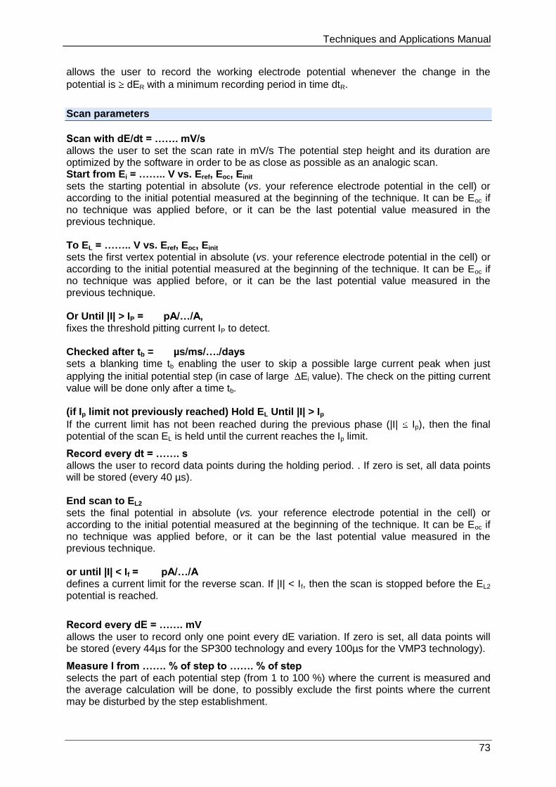
Techniques and Applications Manual
73
allows the user to record the working electrode potential whenever the change in the
potential is dER with a minimum recording period in time dtR.
Scan parameters
Scan with dE/dt = ……. mV/s allows the user to set the scan rate in mV/s The potential step height and its duration are optimized by the software in order to be as close as possible as an analogic scan. Start from Ei = …….. V vs. Eref, Eoc, Einit sets the starting potential in absolute (vs. your reference electrode potential in the cell) or according to the initial potential measured at the beginning of the technique. It can be Eoc if no technique was applied before, or it can be the last potential value measured in the previous technique. To EL = …….. V vs. Eref, Eoc, Einit sets the first vertex potential in absolute (vs. your reference electrode potential in the cell) or according to the initial potential measured at the beginning of the technique. It can be Eoc if no technique was applied before, or it can be the last potential value measured in the previous technique. Or Until |I| > IP = pA/…/A, fixes the threshold pitting current IP to detect. Checked after tb = µs/ms/…./days sets a blanking time tb enabling the user to skip a possible large current peak when just
applying the initial potential step (in case of large Ei value). The check on the pitting current value will be done only after a time tb. (if Ip limit not previously reached) Hold EL Until |I| > Ip
If the current limit has not been reached during the previous phase (|I| Ip), then the final potential of the scan EL is held until the current reaches the Ip limit.
Record every dt = ……. s allows the user to record data points during the holding period. . If zero is set, all data points will be stored (every 40 µs). End scan to EL2 sets the final potential in absolute (vs. your reference electrode potential in the cell) or according to the initial potential measured at the beginning of the technique. It can be Eoc if no technique was applied before, or it can be the last potential value measured in the previous technique. or until |I| < If = pA/…/A defines a current limit for the reverse scan. If |I| < If, then the scan is stopped before the EL2 potential is reached.
Record every dE = ……. mV allows the user to record only one point every dE variation. If zero is set, all data points will be stored (every 44µs for the SP300 technology and every 100µs for the VMP3 technology).
Measure I from ……. % of step to ……. % of step selects the part of each potential step (from 1 to 100 %) where the current is measured and the average calculation will be done, to possibly exclude the first points where the current may be disturbed by the step establishment.
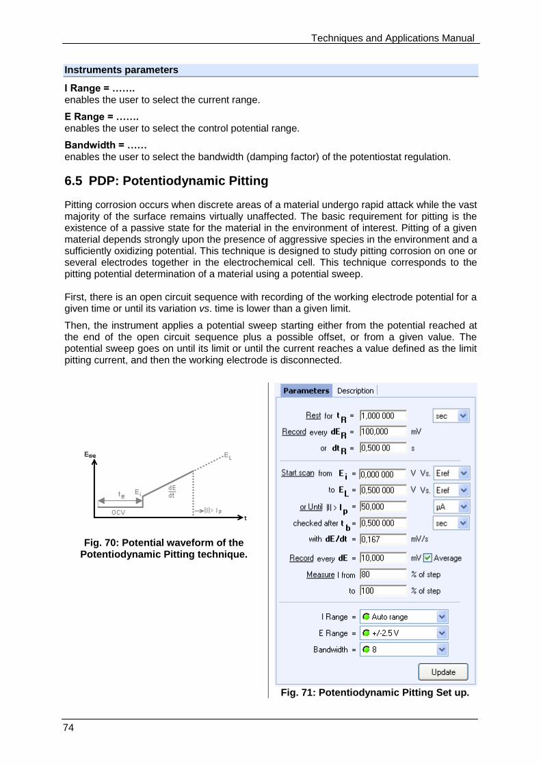
Techniques and Applications Manual
74
Instruments parameters
I Range = ……. enables the user to select the current range.
E Range = ……. enables the user to select the control potential range.
Bandwidth = …… enables the user to select the bandwidth (damping factor) of the potentiostat regulation.
6.5 PDP: Potentiodynamic Pitting
Pitting corrosion occurs when discrete areas of a material undergo rapid attack while the vast majority of the surface remains virtually unaffected. The basic requirement for pitting is the existence of a passive state for the material in the environment of interest. Pitting of a given material depends strongly upon the presence of aggressive species in the environment and a sufficiently oxidizing potential. This technique is designed to study pitting corrosion on one or several electrodes together in the electrochemical cell. This technique corresponds to the pitting potential determination of a material using a potential sweep. First, there is an open circuit sequence with recording of the working electrode potential for a given time or until its variation vs. time is lower than a given limit.
Then, the instrument applies a potential sweep starting either from the potential reached at the end of the open circuit sequence plus a possible offset, or from a given value. The potential sweep goes on until its limit or until the current reaches a value defined as the limit pitting current, and then the working electrode is disconnected.
Fig. 70: Potential waveform of the Potentiodynamic Pitting technique.
Fig. 71: Potentiodynamic Pitting Set up.
Techniques and Applications Manual
75
Open circuit parameters
Rest for tR = µs/ms/…./days fixes a defined time duration tR for recording the rest potential.
Record every dER = mV
or dtR = s allows the user to record the working electrode potential whenever the change in the
potential is dER with a minimum recording period in time dtR.
Scan parameters
Start scan from Ei = …….. V vs. Eref, Eoc, Einit sets the starting potential in absolute (vs. your reference electrode potential in the cell) or according to the open circuit potential (Eoc) or relatively to the initial potential measured at the beginning of the technique (Einit). Einit can be Eoc if no technique was previously applied or it can be the last potential value measured in the previous technique. To EL = …….. V vs. Eref, Eoc, Einit sets the final potential in absolute (vs. your reference electrode potential in the cell) or according to the open circuit potential (Eoc) or relatively to the initial potential measured at the beginning of the technique (Einit). Einit can be Eoc if no technique was previously applied or it can be the last potential value measured in the previous technique. Or Until |I| > IP = pA/…/A, fixes the threshold pitting current IP to detect. Once the threshold pitting current is reached, the working electrode is disconnected. Checked after tb = µs/ms/…./days sets a blanking time tb enabling the user to skip a possible large current peak when just
applying the initial potential step (in case of large Ei value). The check on the pitting current value will be done only after a time tb. Scan with dE/dt = ……. mV/s allows the user to set the scan rate in mV/s The potential step height and its duration are optimized by the software in order to be as close as possible to an analogic scan.
Record every dE = ……. mV allows the user to record only one point every dE variation. If zero is set, all data points will be stored (every 40 µs).
Measure I from ……. % of step to ……. % of step selects the part of each potential step (from 1 to 100 %) where the current is measured and the average calculation will be done, to possibly exclude the first points where the current may be disturbed by the step establishment. Instruments parameters
I Range = ……. enables the user to select the current range.
E Range = ……. enables the user to select the control potential range.
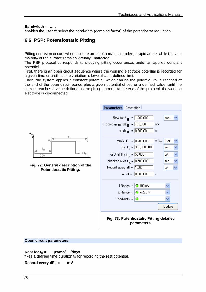
Techniques and Applications Manual
76
Bandwidth = …… enables the user to select the bandwidth (damping factor) of the potentiostat regulation.
6.6 PSP: Potentiostatic Pitting
Pitting corrosion occurs when discrete areas of a material undergo rapid attack while the vast majority of the surface remains virtually unaffected. The PSP protocol corresponds to studying pitting occurrences under an applied constant potential. First, there is an open circuit sequence where the working electrode potential is recorded for a given time or until its time variation is lower than a defined limit. Then, the system applies a constant potential, which can be the potential value reached at the end of the open circuit period plus a given potential offset, or a defined value, until the current reaches a value defined as the pitting current. At the end of the protocol, the working electrode is disconnected.
Fig. 72: General description of the Potentiostatic Pitting.
Fig. 73: Potentiostatic Pitting detailed parameters.
Open circuit parameters
Rest for tR = µs/ms/…./days fixes a defined time duration tR for recording the rest potential.
Record every dER = mV
Techniques and Applications Manual
77
or dtR = s allows the user to record the working electrode potential whenever the change in the
potential is dER with a minimum recording period in time dtR.
Scan parameters
Apply Ei = …….. V vs. Eref, Eoc, Einit sets the potential to a fixed value E (vs. Ref, the reference electrode potential in the cell) or according to the open circuit potential (Eoc) or relatively to the initial potential measured at the beginning of the technique (Einit). Einit can be Eoc if no technique was previously applied or it can be the last potential value measured in the previous technique. For ti = …….. µs/ms/…./days sets the potential step duration. Or Until |I| > IP = pA/…/A, fixes the threshold pitting current IP to detect. Once the threshold pitting current is reached, the working electrode is disconnected. Checked after tb = µs/ms/…./days sets a blanking time tb enabling the user to skip a possible large current peak when just
applying the initial potential step (in case of large Ei value). The check on the pitting current value will be done only after a time tb.
Record every dI = ……. pA/…/A or dt= …... s allows the user to record only one point every dE variation. If zero is set, all data points will be stored (every 24 µs).
Measure I from ……. % of step to ……. % of step selects the part of each potential step (from 1 to 100 %) where the current is measured and the average calculation will be done, to possibly exclude the first points where the current may be disturbed by the step establishment. Instruments parameters
I Range = ……. enables the user to select the current range.
E Range = ……. enables the user to select the control potential range. Bandwidth = …… enables the user to select the bandwidth (damping factor) of the potentiostat regulation.
6.7 ZRA: Zero Resistance Ammeter
The Zero Resistance Ammeter is an application for the measurement of galvanic coupling current of dissimilar metals. It is also made to perform some types of electrochemical noise measurement. It consists into applying zero volts between the working electrode (WE) and the counter electrode (CE) and then measuring the current and the potentials (Ewe, Ece) versus the reference electrode (REF). In most of the cases the coupling current is measured between two identical electrodes. In real situations the electrodes are slightly different resulting in an anodic behavior for one of them and in a cathodic behavior for the other one.
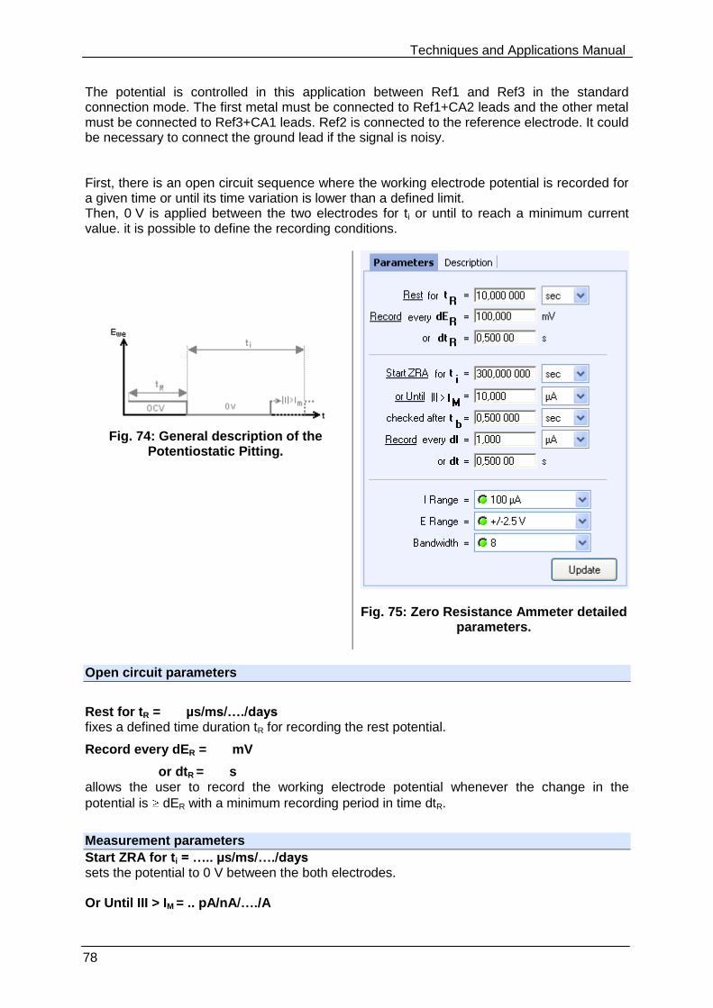
Techniques and Applications Manual
78
The potential is controlled in this application between Ref1 and Ref3 in the standard connection mode. The first metal must be connected to Ref1+CA2 leads and the other metal must be connected to Ref3+CA1 leads. Ref2 is connected to the reference electrode. It could be necessary to connect the ground lead if the signal is noisy. First, there is an open circuit sequence where the working electrode potential is recorded for a given time or until its time variation is lower than a defined limit. Then, 0 V is applied between the two electrodes for ti or until to reach a minimum current value. it is possible to define the recording conditions.
Fig. 74: General description of the
Potentiostatic Pitting.
Fig. 75: Zero Resistance Ammeter detailed parameters.
Open circuit parameters
Rest for tR = µs/ms/…./days fixes a defined time duration tR for recording the rest potential.
Record every dER = mV
or dtR = s allows the user to record the working electrode potential whenever the change in the
potential is dER with a minimum recording period in time dtR.
Measurement parameters
Start ZRA for ti = ….. µs/ms/…./days sets the potential to 0 V between the both electrodes. Or Until III > IM = .. pA/nA/…./A
Techniques and Applications Manual
79
sets the potential step duration. Checked after tb …… µs/ms/…./days sets a blanking time tb enabling the user to skip a possible large current peak when just
applying the initial potential step (in case of large Ei value). The check on the pitting current value will be done only after a time tb. Record every dI = ……. pA/nA/…./A or dt= …... s allows the user to record only one point every dE variation. If zero is set, all data points will be stored (every 40 µs). Instruments parameters
I Range = ……. enables the user to select the current range.
E Range = ……. enables the user to select the control potential range. Bandwidth = …… enables the user to select the bandwidth (damping factor) of the potentiostat regulation.
6.8 CASG: Constant Amplitude sinusoidal micro-Galvanopolarisation
Constant Amplitude Sinusoidal micro Galvano polarization (CASG) is a technique performed on an electrochemical system by applying a current perturbation at a fixed frequency fs. The perturbation is performed around an initial current (Ii) with a small amplitude (Ia) and a constant low frequency (fs).Thanks to a Direct Fourier Transform the amplitudes of the fundamental frequency (fs), 1st (2 fs) and 2nd (3 fs) harmonics are determined. This technique can also be used for other applications such as battery, fuel cell, …
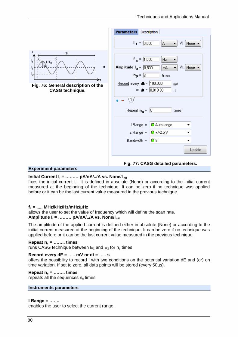
Techniques and Applications Manual
80
Fig. 76: General description of the
CASG technique.
Fig. 77: CASG detailed parameters. Experiment parameters
Initial Current Ii = ……… pA/nA/../A vs. None/Iinit fixes the initial current Ii.. It is defined in absolute (None) or according to the initial current measured at the beginning of the technique. It can be zero if no technique was applied before or it can be the last current value measured in the previous technique. fs = ..... MHz/kHz/Hz/mHz/µHz allows the user to set the value of frequency which will define the scan rate. Amplitude Ii = ……… pA/nA/../A vs. None/Iinit
The amplitude of the applied current is defined either in absolute (None) or according to the initial current measured at the beginning of the technique. It can be zero if no technique was applied before or it can be the last current value measured in the previous technique.
Repeat nc = …….. times runs CASG technique between E1 and E2 for np times
Record every dE = ….. mV or dt = ….. s offers the possibility to record I with two conditions on the potential variation dE and (or) on time variation. If set to zero, all data points will be stored (every 50µs).
Repeat nc = …….. times repeats all the sequences nc times. Instruments parameters
I Range = ……. enables the user to select the current range.
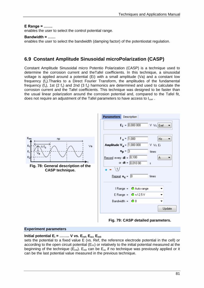
Techniques and Applications Manual
81
E Range = ……. enables the user to select the control potential range.
Bandwidth = …… enables the user to select the bandwidth (damping factor) of the potentiostat regulation.
6.9 Constant Amplitude Sinusoidal microPolarization (CASP)
Constant Amplitude Sinusoidal micro Potentio Polarization (CASP) is a technique used to determine the corrosion current and theTafel coefficients. In this technique, a sinusoidal voltage is applied around a potential (Ei) with a small amplitude (Va) and a constant low frequency (fs).Thanks to a Direct Fourier Transform, the amplitudes of the fundamental frequency (fs), 1st (2 fs) and 2nd (3 fs) harmonics are determined and used to calculate the corrosion current and the Tafel coefficients. This technique was designed to be faster than the usual linear polarization around the corrosion potential and, compared to the Tafel fit, does not require an adjustment of the Tafel parameters to have access to Icorr .
Fig. 78: General description of the
CASP technique.
Fig. 79: CASP detailed parameters. Experiment parameters
Initial potential Ei = …….. V vs. Eref, Eoc, Einit sets the potential to a fixed value E (vs. Ref, the reference electrode potential in the cell) or according to the open circuit potential (Eoc) or relatively to the initial potential measured at the beginning of the technique (Einit). Einit can be Eoc if no technique was previously applied or it can be the last potential value measured in the previous technique.
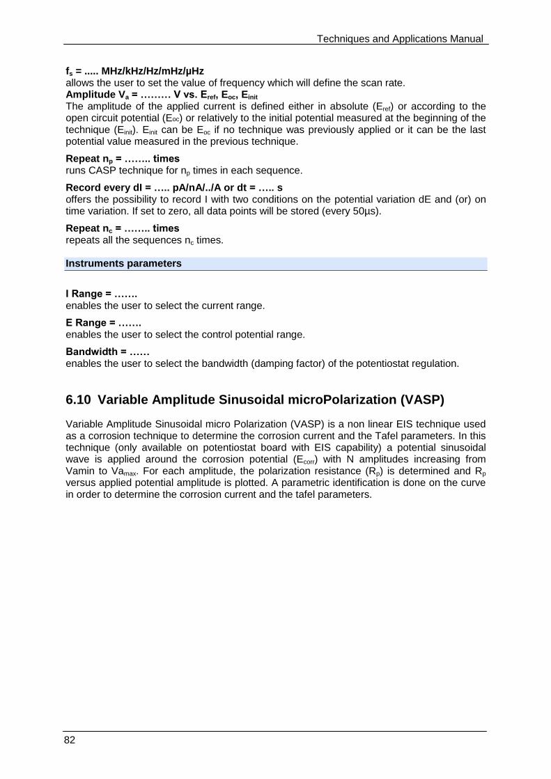
Techniques and Applications Manual
82
fs = ..... MHz/kHz/Hz/mHz/µHz allows the user to set the value of frequency which will define the scan rate. Amplitude Va = ……… V vs. Eref, Eoc, Einit The amplitude of the applied current is defined either in absolute (Eref) or according to the open circuit potential (Eoc) or relatively to the initial potential measured at the beginning of the technique (Einit). Einit can be Eoc if no technique was previously applied or it can be the last potential value measured in the previous technique.
Repeat np = …….. times runs CASP technique for np times in each sequence.
Record every dI = ….. pA/nA/../A or dt = ….. s offers the possibility to record I with two conditions on the potential variation dE and (or) on time variation. If set to zero, all data points will be stored (every 50µs).
Repeat nc = …….. times repeats all the sequences nc times. Instruments parameters
I Range = ……. enables the user to select the current range.
E Range = ……. enables the user to select the control potential range.
Bandwidth = …… enables the user to select the bandwidth (damping factor) of the potentiostat regulation.
6.10 Variable Amplitude Sinusoidal microPolarization (VASP)
Variable Amplitude Sinusoidal micro Polarization (VASP) is a non linear EIS technique used as a corrosion technique to determine the corrosion current and the Tafel parameters. In this technique (only available on potentiostat board with EIS capability) a potential sinusoidal wave is applied around the corrosion potential (Ecorr) with N amplitudes increasing from Vamin to Vamax. For each amplitude, the polarization resistance (Rp) is determined and Rp versus applied potential amplitude is plotted. A parametric identification is done on the curve in order to determine the corrosion current and the tafel parameters.
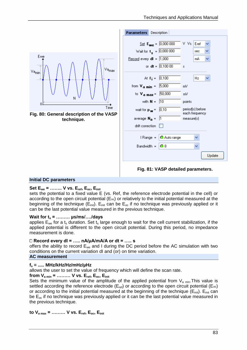
Techniques and Applications Manual
83
Fig. 80: General description of the VASP
technique.
Fig. 81: VASP detailed parameters.
Initial DC parameters
Set Ewe = …….. V vs. Eref, Eoc, Einit sets the potential to a fixed value E (vs. Ref, the reference electrode potential in the cell) or according to the open circuit potential (Eoc) or relatively to the initial potential measured at the beginning of the technique (Einit). Einit can be Eoc if no technique was previously applied or it can be the last potential value measured in the previous technique.
Wait for ts = ……… µs/ms/…./days applies Ewe for a ts duration. Set ts large enough to wait for the cell current stabilization, if the applied potential is different to the open circuit potential. During this period, no impedance measurement is done.
Record every dI = ….. nA/µA/mA/A or dt = ….. s offers the ability to record Ewe and I during the DC period before the AC simulation with two conditions on the current variation dI and (or) on time variation. AC measurement
fs = ..... MHz/kHz/Hz/mHz/µHz allows the user to set the value of frequency which will define the scan rate. from Va min = ……… V vs. Eref, Eoc, Einit Sets the minimum value of the amplitude of the applied potential from Va min.This value is settled according the reference electrode (Eref) or according to the open circuit potential (Eoc) or according to the initial potential measured at the beginning of the technique (Einit). Einit can be Eoc if no technique was previously applied or it can be the last potential value measured in the previous technique. to Va max = ……… V vs. Eref, Eoc, Einit
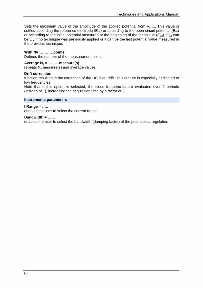
Techniques and Applications Manual
84
Sets the maximum value of the amplitude of the applied potential from Va max.This value is settled according the reference electrode (Eref) or according to the open circuit potential (Eoc) or according to the initial potential measured at the beginning of the technique (Einit). Einit can be Eoc if no technique was previously applied or it can be the last potential value measured in the previous technique. With N=…………points Defines the number of the measurement points
Average Na = …….. measure(s) repeats Na measure(s) and average values.
Drift correction function resulting in the correction of the DC level drift. This feature is especially dedicated to low frequencies. Note that if this option is selected, the sinus frequencies are evaluated over 2 periods (instead of 1), increasing the acquisition time by a factor of 2. Instruments parameters
I Range = ……. enables the user to select the current range.
Bandwidth = …… enables the user to select the bandwidth (damping factor) of the potentiostat regulation
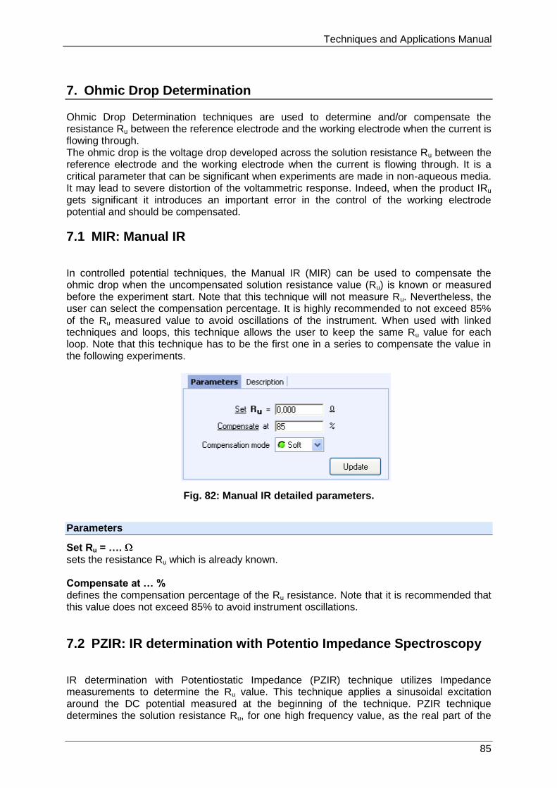
Techniques and Applications Manual
85
7. Ohmic Drop Determination
Ohmic Drop Determination techniques are used to determine and/or compensate the resistance Ru between the reference electrode and the working electrode when the current is flowing through. The ohmic drop is the voltage drop developed across the solution resistance Ru between the reference electrode and the working electrode when the current is flowing through. It is a critical parameter that can be significant when experiments are made in non-aqueous media. It may lead to severe distortion of the voltammetric response. Indeed, when the product IRu gets significant it introduces an important error in the control of the working electrode potential and should be compensated.
7.1 MIR: Manual IR
In controlled potential techniques, the Manual IR (MIR) can be used to compensate the ohmic drop when the uncompensated solution resistance value (Ru) is known or measured before the experiment start. Note that this technique will not measure Ru. Nevertheless, the user can select the compensation percentage. It is highly recommended to not exceed 85% of the Ru measured value to avoid oscillations of the instrument. When used with linked techniques and loops, this technique allows the user to keep the same Ru value for each loop. Note that this technique has to be the first one in a series to compensate the value in the following experiments.
Fig. 82: Manual IR detailed parameters.
Parameters
Set Ru = …. sets the resistance Ru which is already known. Compensate at … % defines the compensation percentage of the Ru resistance. Note that it is recommended that this value does not exceed 85% to avoid instrument oscillations.
7.2 PZIR: IR determination with Potentio Impedance Spectroscopy
IR determination with Potentiostatic Impedance (PZIR) technique utilizes Impedance measurements to determine the Ru value. This technique applies a sinusoidal excitation around the DC potential measured at the beginning of the technique. PZIR technique determines the solution resistance Ru, for one high frequency value, as the real part of the
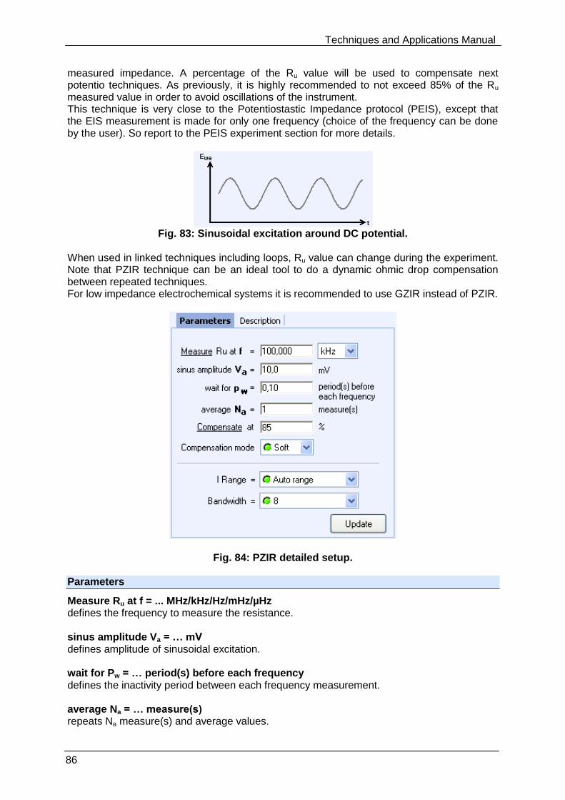
Techniques and Applications Manual
86
measured impedance. A percentage of the Ru value will be used to compensate next potentio techniques. As previously, it is highly recommended to not exceed 85% of the Ru measured value in order to avoid oscillations of the instrument. This technique is very close to the Potentiostastic Impedance protocol (PEIS), except that the EIS measurement is made for only one frequency (choice of the frequency can be done by the user). So report to the PEIS experiment section for more details.
Fig. 83: Sinusoidal excitation around DC potential.
When used in linked techniques including loops, Ru value can change during the experiment. Note that PZIR technique can be an ideal tool to do a dynamic ohmic drop compensation between repeated techniques. For low impedance electrochemical systems it is recommended to use GZIR instead of PZIR.
Fig. 84: PZIR detailed setup.
Parameters
Measure Ru at f = ... MHz/kHz/Hz/mHz/µHz defines the frequency to measure the resistance. sinus amplitude Va = … mV defines amplitude of sinusoidal excitation. wait for Pw = … period(s) before each frequency defines the inactivity period between each frequency measurement. average Na = … measure(s) repeats Na measure(s) and average values.
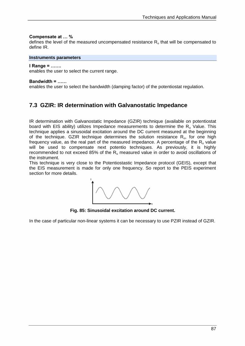
Techniques and Applications Manual
87
Compensate at … % defines the level of the measured uncompensated resistance Ru that will be compensated to define IR. Instruments parameters
I Range = ……. enables the user to select the current range. Bandwidth = …… enables the user to select the bandwidth (damping factor) of the potentiostat regulation.
7.3 GZIR: IR determination with Galvanostatic Impedance
IR determination with Galvanostatic Impedance (GZIR) technique (available on potentiostat board with EIS ability) utilizes Impedance measurements to determine the Ru Value. This technique applies a sinusoidal excitation around the DC current measured at the beginning of the technique. GZIR technique determines the solution resistance Ru, for one high frequency value, as the real part of the measured impedance. A percentage of the Ru value will be used to compensate next potentio techniques. As previously, it is highly recommended to not exceed 85% of the Ru measured value in order to avoid oscillations of the instrument. This technique is very close to the Potentiostastic Impedance protocol (GEIS), except that the EIS measurement is made for only one frequency. So report to the PEIS experiment section for more details.
Fig. 85: Sinusoidal excitation around DC current.
In the case of particular non-linear systems it can be necessary to use PZIR instead of GZIR.
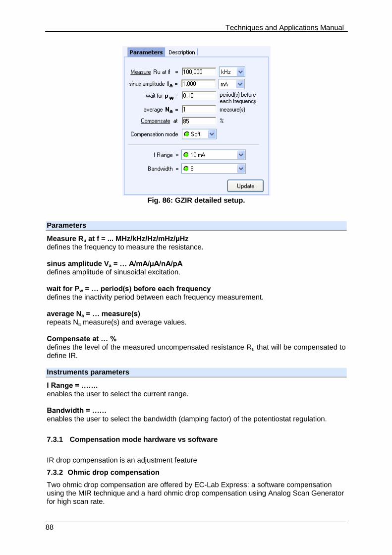
Techniques and Applications Manual
88
Fig. 86: GZIR detailed setup.
Parameters
Measure Ru at f = ... MHz/kHz/Hz/mHz/µHz defines the frequency to measure the resistance. sinus amplitude Va = … A/mA/µA/nA/pA defines amplitude of sinusoidal excitation. wait for Pw = … period(s) before each frequency defines the inactivity period between each frequency measurement. average Na = … measure(s) repeats Na measure(s) and average values. Compensate at … % defines the level of the measured uncompensated resistance Ru that will be compensated to define IR. Instruments parameters
I Range = ……. enables the user to select the current range. Bandwidth = …… enables the user to select the bandwidth (damping factor) of the potentiostat regulation.
7.3.1 Compensation mode hardware vs software
IR drop compensation is an adjustment feature
7.3.2 Ohmic drop compensation
Two ohmic drop compensation are offered by EC-Lab Express: a software compensation using the MIR technique and a hard ohmic drop compensation using Analog Scan Generator for high scan rate.
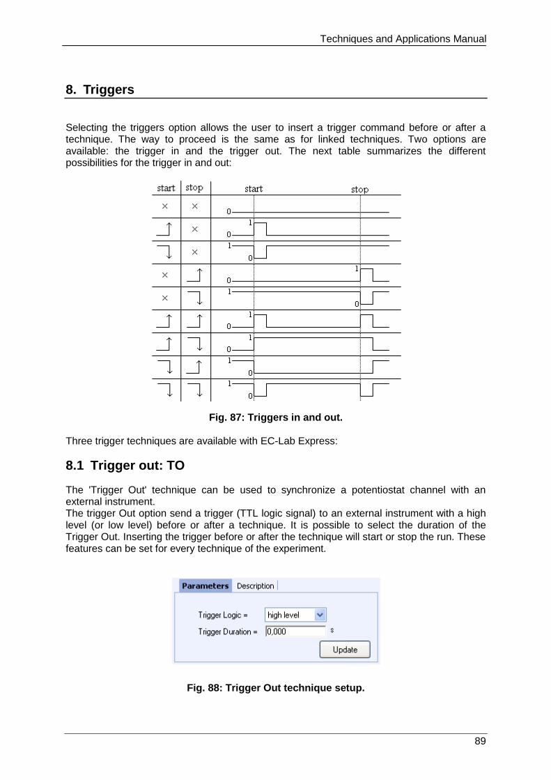
Techniques and Applications Manual
89
8. Triggers
Selecting the triggers option allows the user to insert a trigger command before or after a technique. The way to proceed is the same as for linked techniques. Two options are available: the trigger in and the trigger out. The next table summarizes the different possibilities for the trigger in and out:
Fig. 87: Triggers in and out.
Three trigger techniques are available with EC-Lab Express:
8.1 Trigger out: TO
The 'Trigger Out' technique can be used to synchronize a potentiostat channel with an external instrument. The trigger Out option send a trigger (TTL logic signal) to an external instrument with a high level (or low level) before or after a technique. It is possible to select the duration of the Trigger Out. Inserting the trigger before or after the technique will start or stop the run. These features can be set for every technique of the experiment.
Fig. 88: Trigger Out technique setup.
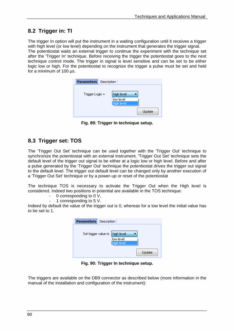
Techniques and Applications Manual
90
8.2 Trigger in: TI
The trigger In option will put the instrument in a waiting configuration until it receives a trigger with high level (or low level) depending on the instrument that generates the trigger signal. The potentiostat waits an external trigger to continue the experiment with the technique set after the 'Trigger In' technique. Before receiving the trigger the potentiostat goes to the next technique control mode. The trigger in signal is level sensitive and can be set to be either logic low or high. For the potentiostat to recognize the trigger a pulse must be set and held for a minimum of 100 µs.
Fig. 89: Trigger In technique setup.
8.3 Trigger set: TOS
The 'Trigger Out Set' technique can be used together with the 'Trigger Out' technique to synchronize the potentiostat with an external instrument. 'Trigger Out Set' technique sets the default level of the trigger out signal to be either at a logic low or high level. Before and after a pulse generated by the 'Trigger Out' technique the potentiostat drives the trigger out signal to the default level. The trigger out default level can be changed only by another execution of a 'Trigger Out Set' technique or by a power-up or reset of the potentiostat The technique TOS is necessary to activate the Trigger Out when the High level is considered. Indeed two positions in potential are available in the TOS technique:
- 0 corresponding to 0 V, - 1 corresponding to 5 V.
Indeed by default the value of the trigger out is 0, whereas for a low level the initial value has to be set to 1.
Fig. 90: Trigger In technique setup.
The triggers are available on the DB9 connector as described below (more information in the manual of the installation and configuration of the instrument):
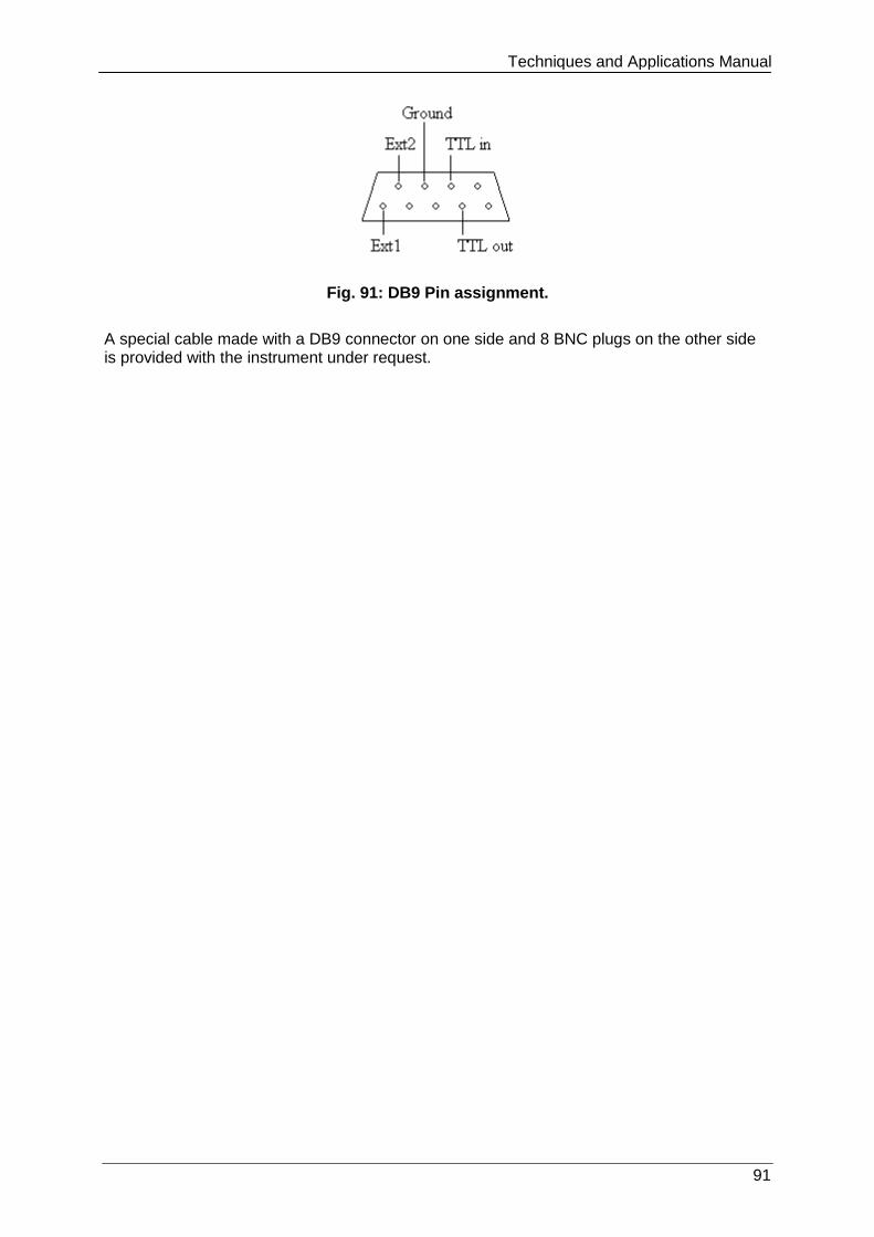
Techniques and Applications Manual
91
Fig. 91: DB9 Pin assignment.
A special cable made with a DB9 connector on one side and 8 BNC plugs on the other side is provided with the instrument under request.
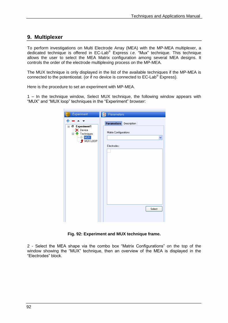
Techniques and Applications Manual
92
9. Multiplexer
To perform investigations on Multi Electrode Array (MEA) with the MP-MEA multiplexer, a dedicated technique is offered in EC-Lab® Express i.e. “Mux” technique. This technique allows the user to select the MEA Matrix configuration among several MEA designs. It controls the order of the electrode multiplexing process on the MP-MEA. The MUX technique is only displayed in the list of the available techniques if the MP-MEA is connected to the potentiostat. (or if no device is connected to EC-Lab® Express). Here is the procedure to set an experiment with MP-MEA. 1 – In the technique window, Select MUX technique, the following window appears with “MUX” and “MUX loop” techniques in the “Experiment” browser:
Fig. 92: Experiment and MUX technique frame.
2 - Select the MEA shape via the combo box “Matrix Configurations” on the top of the window showing the “MUX” technique, then an overview of the MEA is displayed in the “Electrodes” block.
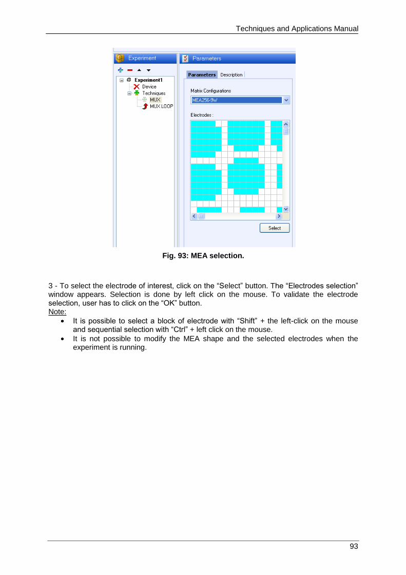
Techniques and Applications Manual
93
Fig. 93: MEA selection.
3 - To select the electrode of interest, click on the “Select” button. The “Electrodes selection” window appears. Selection is done by left click on the mouse. To validate the electrode selection, user has to click on the “OK” button. Note:
It is possible to select a block of electrode with “Shift” + the left-click on the mouse and sequential selection with “Ctrl” + left click on the mouse.
It is not possible to modify the MEA shape and the selected electrodes when the experiment is running.
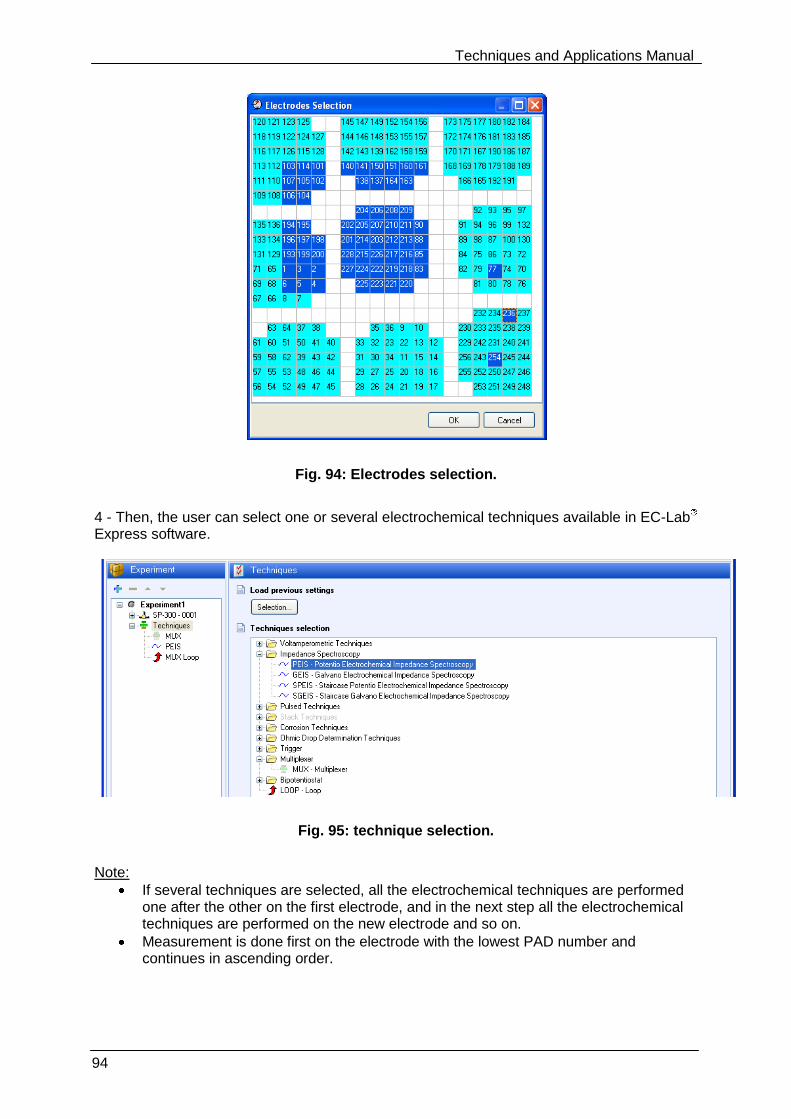
Techniques and Applications Manual
94
Fig. 94: Electrodes selection.
4 - Then, the user can select one or several electrochemical techniques available in EC-Lab Express software.
Fig. 95: technique selection.
Note:
If several techniques are selected, all the electrochemical techniques are performed one after the other on the first electrode, and in the next step all the electrochemical techniques are performed on the new electrode and so on.
Measurement is done first on the electrode with the lowest PAD number and continues in ascending order.
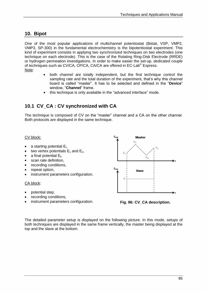
Techniques and Applications Manual
95
10. Bipot
One of the most popular applications of multichannel potentiostat (Bistat, VSP, VMP2, VMP3, SP-300) in the fundamental electrochemistry is the bipotentiostat experiment. This kind of experiment consists in applying two synchronized techniques on two electrodes (one technique on each electrode). This is the case of the Rotating Ring-Disk Electrode (RRDE) or hydrogen permeation investigations. In order to make easier the set-up, dedicated couple of techniques such as CV/CA, CP/CA, CA/CA are offered in EC-Lab® Express. Note:
both channel are totally independent, but the first technique control the sampling rate and the total duration of the experiment, that’s why this channel board is called “master”. It has to be selected and defined in the “Device” window, “Channel” frame.
this technique is only available in the “advanced interface” mode.
10.1 CV_CA : CV synchronized with CA
The technique is composed of CV on the “master” channel and a CA on the other channel. Both protocols are displayed in the same technique. CV block:
a starting potential Ei,
two vertex potentials E1 and E2,
a final potential Ef,
scan rate definition,
recording conditions,
repeat option,
instrument parameters configuration. CA block:
potential step,
recording conditions,
instrument parameters configuration.
Fig. 96: CV_CA description.
The detailed parameter setup is displayed on the following picture. In this mode, setups of both techniques are displayed in the same frame vertically, the master being displayed at the top and the slave at the bottom.
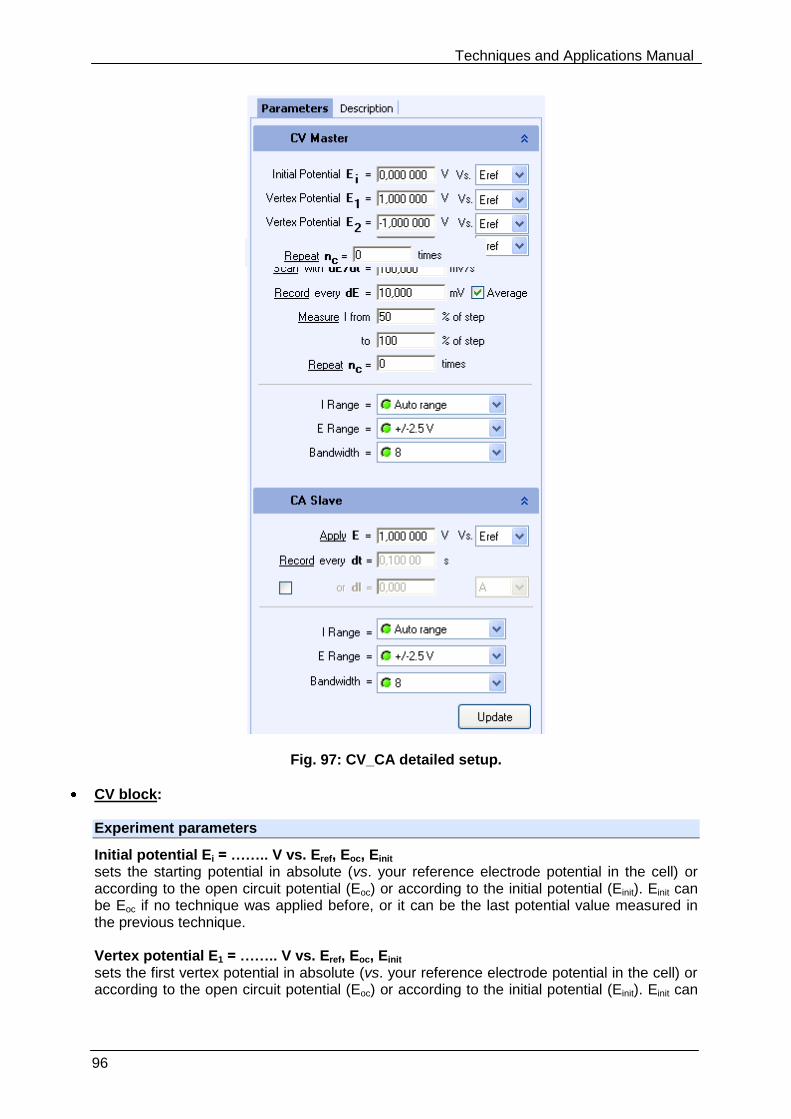
Techniques and Applications Manual
96
Fig. 97: CV_CA detailed setup.
CV block:
Experiment parameters
Initial potential Ei = …….. V vs. Eref, Eoc, Einit sets the starting potential in absolute (vs. your reference electrode potential in the cell) or according to the open circuit potential (Eoc) or according to the initial potential (Einit). Einit can be Eoc if no technique was applied before, or it can be the last potential value measured in the previous technique. Vertex potential E1 = …….. V vs. Eref, Eoc, Einit sets the first vertex potential in absolute (vs. your reference electrode potential in the cell) or according to the open circuit potential (Eoc) or according to the initial potential (Einit). Einit can
Techniques and Applications Manual
97
be Eoc if no technique was applied before, or it can be the last potential value measured in the previous technique Vertex potential E2 = …….. V vs. Eref, Eoc, Einit sets the second vertex potential in absolute (vs. your reference electrode potential in the cell) or according to the open circuit potential (Eoc) or according to the initial potential (Einit). Einit can be Eoc if no technique was applied before, or it can be the last potential value measured in the previous technique Final potential Ef = …….. V vs. Eref, Eoc, Einit sets the final potential in absolute (vs. your reference electrode potential in the cell) or according to the open circuit potential (Eoc) or according to the initial potential (Einit). Einit can be Eoc if no technique was applied before, or it can be the last potential value measured in the previous technique . Scan with dE/dt = ……. mV/s allows the user to set the scan rate in mV/s The potential step height and its duration are optimized by the software in order to be as close as possible as an analogic scan.
Record every dE = ……. mV allows the user to record only one point every dE variation. If set to zero, all data points will be stored (every 50 µs). [] Average if this box is ticked, an average on the potential is done every dE previously defined.
Measure I from ……. % of step to ……. % of step selects the part of each potential step (from 1 to 100%) where the current is measured and the average calculation will be done, to possibly exclude the first points where the current may be disturbed by the step establishment.
Repeat nc = …….. times runs cyclic voltammetry between E1 and E2 for nc times Instruments parameters
I Range = ……. enables the user to select the current range.
E Range = ……. enables the user to select the control potential range.
Bandwidth = …… enables the user to select the bandwidth (damping factor) of the potentiostat regulation.
CA block:
Experiment parameters
Apply E = ………… V vs. Eref, Eoc, Einit the applied potential is defined in absolute (vs. your reference electrode potential in the cell) or according to the open circuit potential (Eoc) or according to the initial potential measured at the beginning of the technique. It can be Eoc if no technique was applied before, or it can be the last potential value measured in the previous technique.
Record I every dt = …. s (or dI = …. pA/…/A; optional)
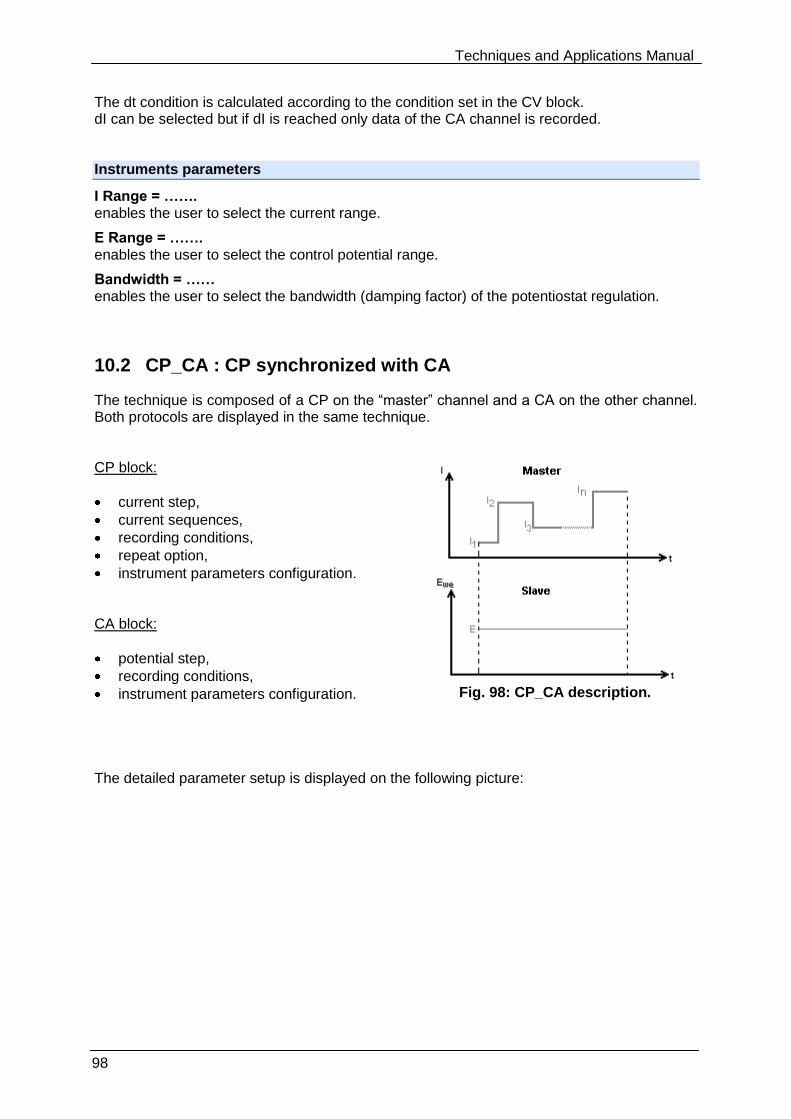
Techniques and Applications Manual
98
The dt condition is calculated according to the condition set in the CV block. dI can be selected but if dI is reached only data of the CA channel is recorded. Instruments parameters
I Range = ……. enables the user to select the current range.
E Range = ……. enables the user to select the control potential range.
Bandwidth = …… enables the user to select the bandwidth (damping factor) of the potentiostat regulation.
10.2 CP_CA : CP synchronized with CA
The technique is composed of a CP on the “master” channel and a CA on the other channel. Both protocols are displayed in the same technique. CP block:
current step,
current sequences,
recording conditions,
repeat option,
instrument parameters configuration.
CA block:
potential step,
recording conditions,
instrument parameters configuration.
Fig. 98: CP_CA description.
The detailed parameter setup is displayed on the following picture:
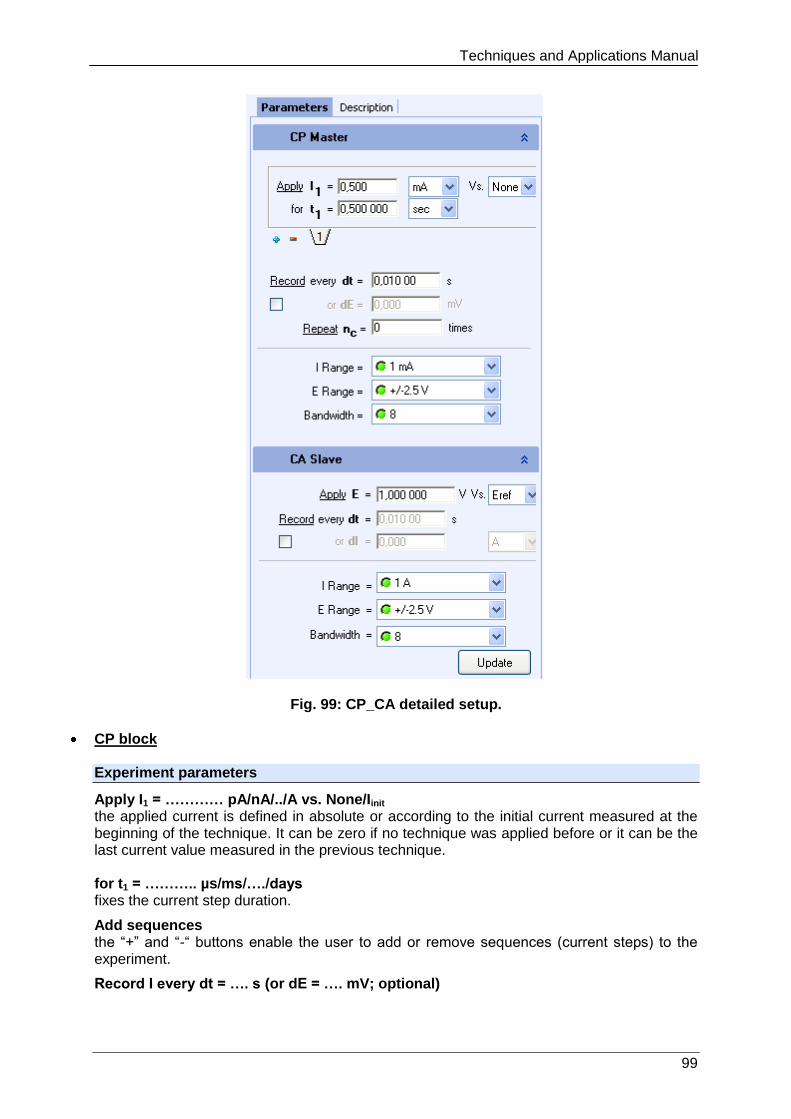
Techniques and Applications Manual
99
Fig. 99: CP_CA detailed setup.
CP block
Experiment parameters
Apply I1 = ………… pA/nA/../A vs. None/Iinit the applied current is defined in absolute or according to the initial current measured at the beginning of the technique. It can be zero if no technique was applied before or it can be the last current value measured in the previous technique. for t1 = ……….. µs/ms/…./days fixes the current step duration.
Add sequences the “+” and “-“ buttons enable the user to add or remove sequences (current steps) to the experiment.
Record I every dt = …. s (or dE = …. mV; optional)
Techniques and Applications Manual
100
The dt condition is applied to both technique of the CP_CA technique. So sampling rate of both techniques are synchronized. If zero is set, all data points will be stored (every 24 µs). dE can be selected but if dE is reached only data of the CP channel are recorded.
Repeat nc = …….. times runs current sequences for nc times. Instruments parameters
I Range = ……. enables the user to select the current range.
E Range = ……. enables the user to select the control potential range.
Bandwidth = …… enables the user to select the bandwidth (damping factor) of the potentiostat regulation.
CA block
Experiment parameters
Apply E = ………… V vs. Eref, Eoc, Einit the applied potential is defined in absolute (vs. your reference electrode potential in the cell) or according to the open circuit potential (Eoc) or according to the initial potential measured at the beginning of the technique. It can be Eoc if no technique was previously applied, or it can be the last potential value measured in the previous technique.
Record I every dt = …. s (or dI = …. pA/…/A; optional) The dt condition is the dt set in the CP block. dI can be selected but if dI is reached only data of the CA channel is recorded. Instruments parameters
I Range = ……. enables the user to select the current range.
E Range = ……. enables the user to select the control potential range.
Bandwidth = …… enables the user to select the bandwidth (damping factor) of the potentiostat regulation.
10.3 CA_CA : CA synchonized with CA
The technique is composed of two CA one on the “master” channel and another of the other channel. Both protocols are displayed in the same technique. The detailed flow diagram is made as follows:
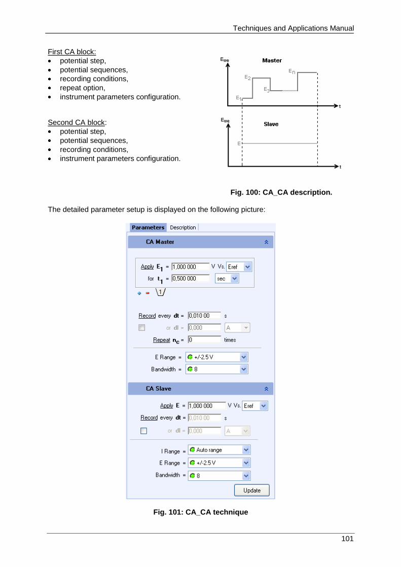
Techniques and Applications Manual
101
First CA block:
potential step,
potential sequences,
recording conditions,
repeat option,
instrument parameters configuration. Second CA block:
potential step,
potential sequences,
recording conditions,
instrument parameters configuration.
Fig. 100: CA_CA description. The detailed parameter setup is displayed on the following picture:
Fig. 101: CA_CA technique
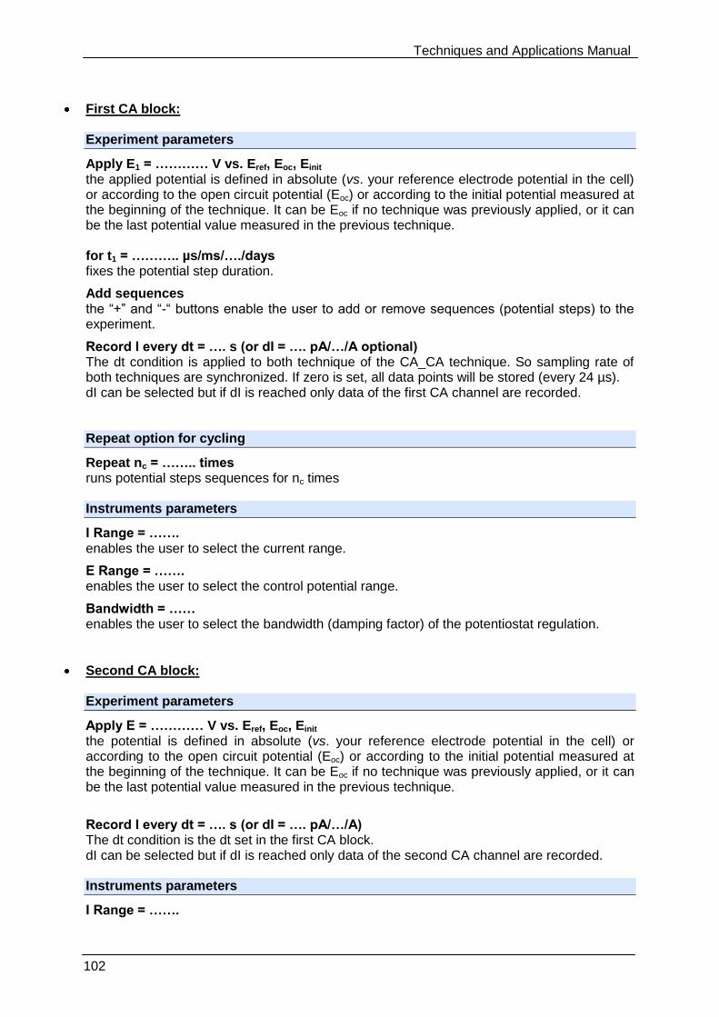
Techniques and Applications Manual
102
First CA block:
Experiment parameters
Apply E1 = ………… V vs. Eref, Eoc, Einit the applied potential is defined in absolute (vs. your reference electrode potential in the cell) or according to the open circuit potential (Eoc) or according to the initial potential measured at the beginning of the technique. It can be Eoc if no technique was previously applied, or it can be the last potential value measured in the previous technique. for t1 = ……….. µs/ms/…./days fixes the potential step duration.
Add sequences the “+” and “-“ buttons enable the user to add or remove sequences (potential steps) to the experiment.
Record I every dt = …. s (or dI = …. pA/…/A optional) The dt condition is applied to both technique of the CA_CA technique. So sampling rate of both techniques are synchronized. If zero is set, all data points will be stored (every 24 µs). dI can be selected but if dI is reached only data of the first CA channel are recorded. Repeat option for cycling
Repeat nc = …….. times runs potential steps sequences for nc times Instruments parameters
I Range = ……. enables the user to select the current range.
E Range = ……. enables the user to select the control potential range.
Bandwidth = …… enables the user to select the bandwidth (damping factor) of the potentiostat regulation.
Second CA block:
Experiment parameters
Apply E = ………… V vs. Eref, Eoc, Einit the potential is defined in absolute (vs. your reference electrode potential in the cell) or according to the open circuit potential (Eoc) or according to the initial potential measured at the beginning of the technique. It can be Eoc if no technique was previously applied, or it can be the last potential value measured in the previous technique.
Record I every dt = …. s (or dI = …. pA/…/A) The dt condition is the dt set in the first CA block. dI can be selected but if dI is reached only data of the second CA channel are recorded. Instruments parameters
I Range = …….

Techniques and Applications Manual
103
enables the user to select the current range.
E Range = ……. enables the user to select the control potential range.
Bandwidth = …… enables the user to select the bandwidth (damping factor) of the potentiostat regulation.
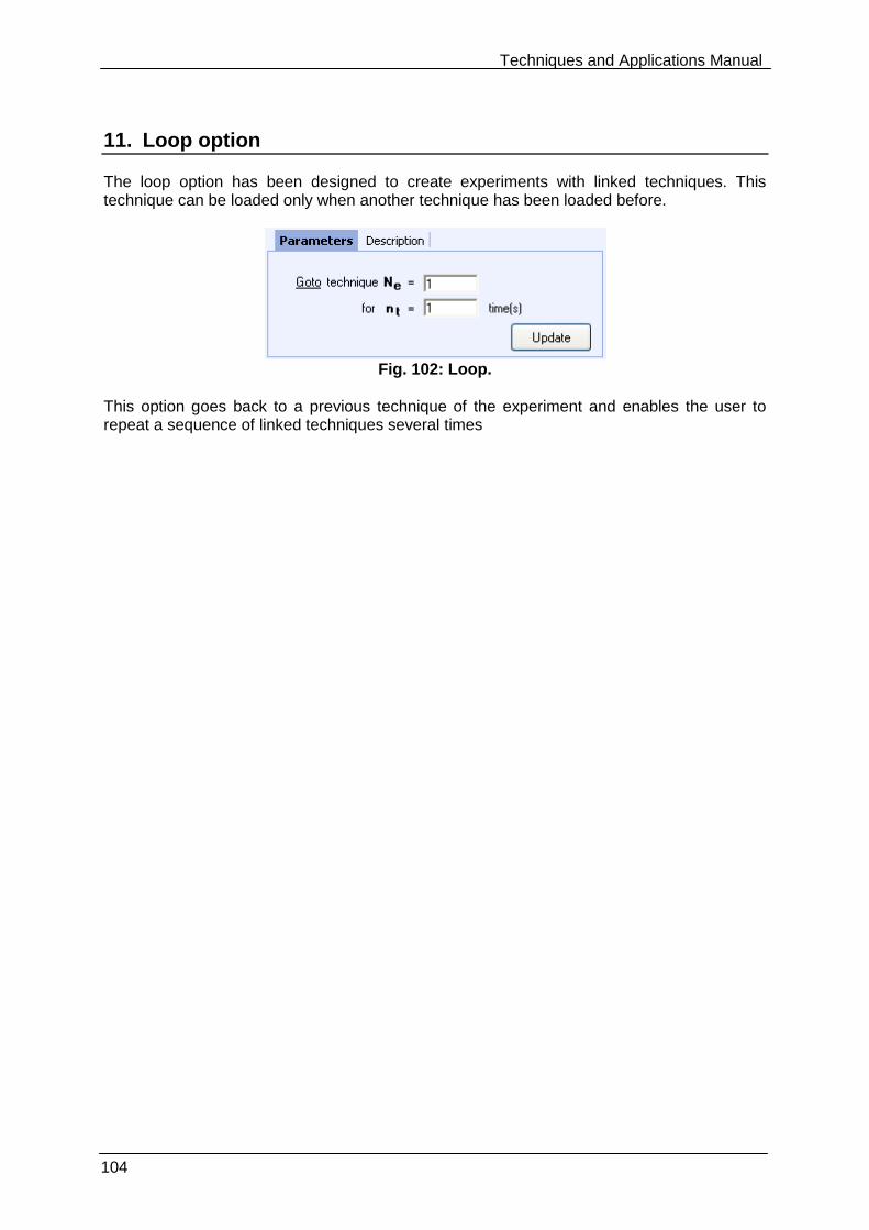
Techniques and Applications Manual
104
11. Loop option
The loop option has been designed to create experiments with linked techniques. This technique can be loaded only when another technique has been loaded before.
Fig. 102: Loop.
This option goes back to a previous technique of the experiment and enables the user to repeat a sequence of linked techniques several times
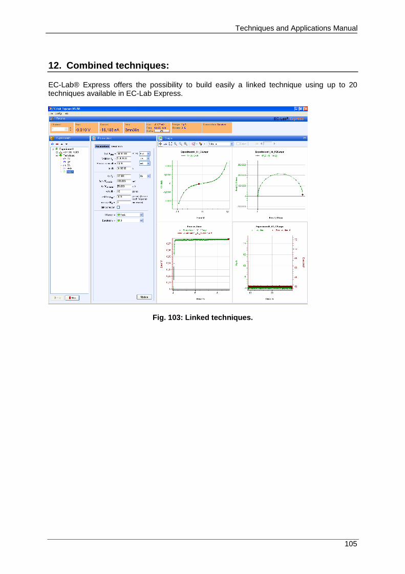
Techniques and Applications Manual
105
12. Combined techniques:
EC-Lab® Express offers the possibility to build easily a linked technique using up to 20 techniques available in EC-Lab Express.
Fig. 103: Linked techniques.
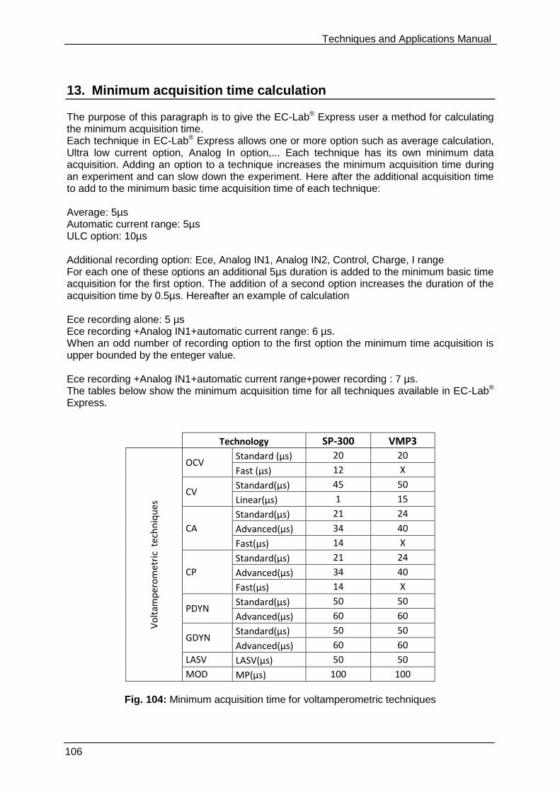
Techniques and Applications Manual
106
13. Minimum acquisition time calculation
The purpose of this paragraph is to give the EC-Lab® Express user a method for calculating the minimum acquisition time. Each technique in EC-Lab® Express allows one or more option such as average calculation, Ultra low current option, Analog In option,... Each technique has its own minimum data acquisition. Adding an option to a technique increases the minimum acquisition time during an experiment and can slow down the experiment. Here after the additional acquisition time to add to the minimum basic time acquisition time of each technique: Average: 5µs Automatic current range: 5µs ULC option: 10µs Additional recording option: Ece, Analog IN1, Analog IN2, Control, Charge, I range For each one of these options an additional 5µs duration is added to the minimum basic time acquisition for the first option. The addition of a second option increases the duration of the acquisition time by 0.5µs. Hereafter an example of calculation Ece recording alone: 5 µs Ece recording +Analog IN1+automatic current range: 6 µs. When an odd number of recording option to the first option the minimum time acquisition is upper bounded by the enteger value. Ece recording +Analog IN1+automatic current range+power recording : 7 µs. The tables below show the minimum acquisition time for all techniques available in EC-Lab® Express.
Technology SP-300 VMP3
Vo
ltam
per
om
etri
c t
ech
niq
ues
OCV Standard (µs) 20 20
Fast (µs) 12 X
CV Standard(µs) 45 50
Linear(µs) 1 15
CA
Standard(µs) 21 24
Advanced(µs) 34 40
Fast(µs) 14 X
CP
Standard(µs) 21 24
Advanced(µs) 34 40
Fast(µs) 14 X
PDYN Standard(µs) 50 50
Advanced(µs) 60 60
GDYN Standard(µs) 50 50
Advanced(µs) 60 60
LASV LASV(µs) 50 50
MOD MP(µs) 100 100
Fig. 104: Minimum acquisition time for voltamperometric techniques
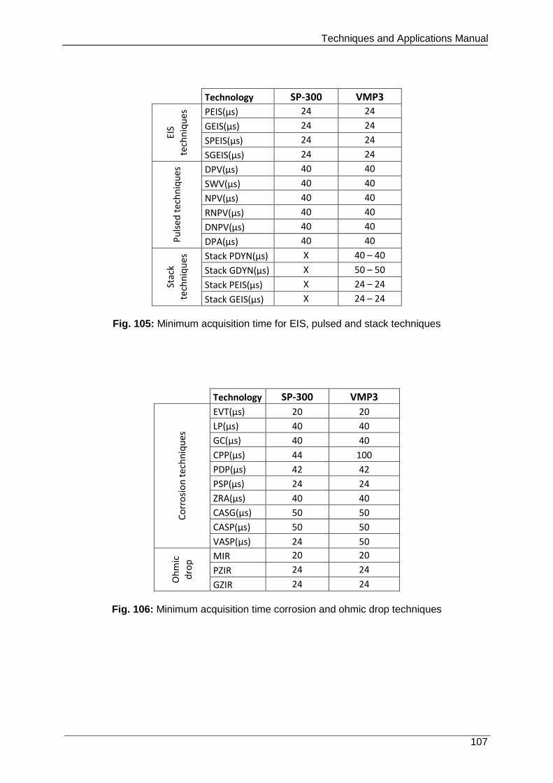
Techniques and Applications Manual
107
Technology SP-300 VMP3
EIS
tech
niq
ues
PEIS(µs) 24 24
GEIS(µs) 24 24
SPEIS(µs) 24 24
SGEIS(µs) 24 24
Pu
lsed
tec
hn
iqu
es
DPV(µs) 40 40
SWV(µs) 40 40
NPV(µs) 40 40
RNPV(µs) 40 40
DNPV(µs) 40 40
DPA(µs) 40 40
Stac
k
tech
niq
ues
Stack PDYN(µs) X 40 – 40
Stack GDYN(µs) X 50 – 50
Stack PEIS(µs) X 24 – 24
Stack GEIS(µs) X 24 – 24
Fig. 105: Minimum acquisition time for EIS, pulsed and stack techniques
Technology SP-300 VMP3
Co
rro
sio
n t
ech
niq
ues
EVT(µs) 20 20
LP(µs) 40 40
GC(µs) 40 40
CPP(µs) 44 100
PDP(µs) 42 42
PSP(µs) 24 24
ZRA(µs) 40 40
CASG(µs) 50 50
CASP(µs) 50 50
VASP(µs) 24 50
Oh
mic
d
rop
MIR 20 20
PZIR 24 24
GZIR 24 24
Fig. 106: Minimum acquisition time corrosion and ohmic drop techniques
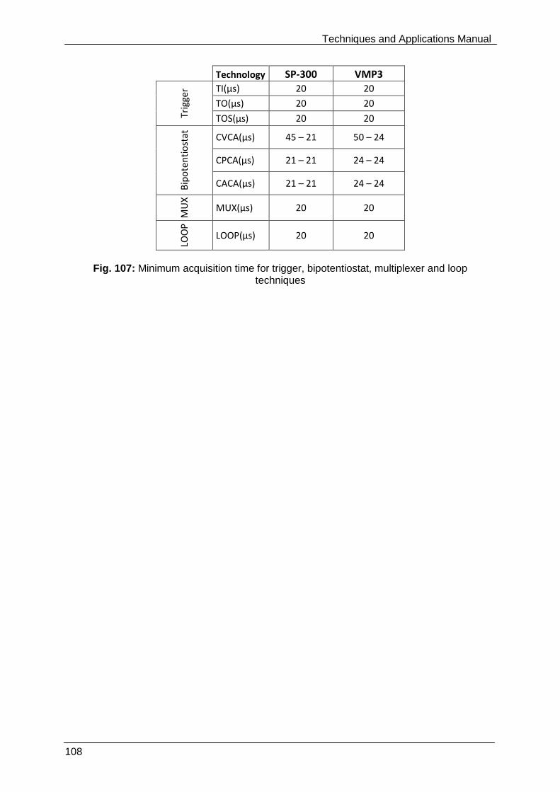
Techniques and Applications Manual
108
Technology SP-300 VMP3
Trig
ger TI(µs) 20 20
TO(µs) 20 20
TOS(µs) 20 20
Bip
ote
nti
ost
at
CVCA(µs) 45 – 21 50 – 24
CPCA(µs) 21 – 21 24 – 24
CACA(µs) 21 – 21 24 – 24 M
UX
MUX(µs) 20 20
LOO
P
LOOP(µs) 20 20
Fig. 107: Minimum acquisition time for trigger, bipotentiostat, multiplexer and loop
techniques
Techniques and Applications Manual
109
14. Glossary
This glossary is made for the user to understand most of the terms of EC-Lab Express software and the terms mentioned in the manual. The terms are classified in the alphabetical order. Absolute value: mathematical function that changes the negative values in positive ones.
Accept: button in EC-Lab Express software that switches to "Modify" when the user clicks on. "Modify" must be displayed to run the experiment. Bandwidth: represents the frequency of the regulation loop of the potentiostat. It depends on the electrochemical cell impedance. The bandwidths values are going from 1 to 7 with increasing frequency. CASP: corrosion protocol used to determine the corrosion current and the Tafel coefficients. In this technique, a sinusoidal voltage is applied around a potential (Ei) with a small amplitude (Va) and a constant low frequency (fs). CASG: corrosion technique performed on an electrochemical system by applying a current perturbation at a fixed frequency fs. The perturbation is performed around an initial current (Ii) with a small amplitude (Ia) and a constant low frequency (fs). Channels: each one of the boards corresponding to an independent Potentiostat/galvanostat. Chronoamperometry/ chronocoulometry: controlled potential technique that consists in stepping the potential of the working electrode from an open circuit potential to another potential Ei where electrochemical reactions occur. The resulting curve is a current-time response. Chronocoulometry is an alternative mode for recording the charged passed as a function of time with current integration. Chronopotentiometry: controlled current technique where the potential is the variable determined as a function of time during a current step. Cycle: inside a protocol, this term is used to describe a sequence repeated with time. Cycle number: processing function that allows the user to display on the graphic one or several cycles chosen in the raw file. The selected cycles are lightened and the others are hidden. Cyclic potentiodynamic pitting (CPP): corrosion protocol used to evaluate pitting susceptibility and made with a potentiodynamic part and a conditional potentiostatic part which is taken into account if the pitting current is not reached during the potentiodynamic part. Cyclic voltammetry (CV): this protocol consists in scanning linearly the potential of the working electrode and to measure the current resulting from oxydoreduction reactions. Cyclic voltammetry provides information on redox processes, electron transfer reactions and adsorption processes.
Techniques and Applications Manual
110
Differential Pulse Voltammetry (DPV): protocol used in analytical electrochemistry to discriminate faradic from capacitive current. This technique consists of pulses superimposed on a potential sweep. Differential Normal Pulse Voltammetry (DNPV): protocol used in analytical electrochemistry to discriminate faradic from capacitive current. This technique is made of increasing prepulses with time and pulses superimposed on the prepulses. Differential pulse amperometry (DPA): protocol used in analytical electrochemistry to discriminate faradic from capacitive current. This technique consists in the repetition of a pulse sequences made with a prepulse and a pulse superimposed. Galvano Electrochemical Impedance Spectroscopy (GEIS): protocol for impedance measurement in a galvanostatic mode. Generalized corrosion (GC): protocol used to study general corrosion. It consists in half a cycle or a cycle of usual cyclic voltammetry with a digital potential sweep. I range: current range used in the experiment. It is related to the current resolution. Impedance: defined by the ratio E/I IR compensation: in the electrochemical cell, the resistance between the working and the reference electrode produces a potential drop that keep the working electrode from being at the controlled potential. IR compensation allows the user to set a resistance value to compensate the solution resistance. Linear polarization (LP): protocol that consists in a potential ramp around the corrosion potential. It is often used to determine polarization resistance and corrosion current.
Linked experiments: EC-Lab Express offers the ability to link up to ten different experiments with the protocol linker. Linked experiment settings: the user can save the settings of linked experiments as a .mpls file. This allows the user to load easily all the experiment settings. Loop: protocol available in the linked experiments and used to repeat one or more experiments. It is different from the cycle in an experiment. Potentiodynamic pitting (PDP): corrosion protocol designed to study pitting corrosion on one electrode in the electrochemical cell. This protocol corresponds to the pitting potential determination of a material using a potential sweep. Potentiostatic pitting (PSP): corrosion protocol designed to study pitting corrosion on one electrode in the electrochemical cell using a potential step. Normal pulse voltammetry (NPV): protocol used in analytical electrochemistry to discriminate faradic from capacitive current. This technique is made of increasing pulses with time that are always coming back to the beginning potential. Open Circuit Voltage (OCV): protocol that consists in a period during which no potential or current is applied to the working electrode. The cell is disconnected and only the potential measurement is available.
Techniques and Applications Manual
111
Pause: Button of EC-Lab Express main window that lead to a suspension in the progress of the protocol and in the measurement recording. The cell is disconnected (OCV period). The "Pause" button switches to "Resume" when clicked. Potentiostatic impedance (PEIS): protocol that performs impedance measurements into potentiostatic mode in applying a sinus around a potential E that can be set to fixed value or relatively to the cell equilibrium potential. Reverse Normal Pulse Voltammetry (RNPV): protocol used in analytical electrochemistry to discriminate faradic from capacitive current. This technique is made of increasing pulses with time that are always coming back to the beginning potential. The current is sampled in the opposite way as for the NPV technique. Run: button that start the experiment. Scan rate: speed of the potential sweep defined with the smallest possible step amplitude Triggers: option that allows the instrument to set a trigger out (TTL signal) at experiment start/stop or to wait for an external trigger in to start or stop the run. Square Wave Voltammetry (SWV): protocol used in analytical electrochemistry to discriminate faradic from capacitive current. This technique is made of successive positive and negative pulses according to the averaged potential sweep. VASP: Variable Amplitude Sinusoidal micro Polarization is a corrosion technique allowing the determination of the corrosion current and the Tafel parameters. This technique is performed by applying a sinusoidal potential wave around the corrosion potential with N amplitudes increasing from Vamin to Vamax. For each amplitude, the polarization resistance (Rp) is determined and Rp versus applied potential amplitude is plotted Zero Resistance Ammeter (ZRA): protocol used to perform measurements to examine the effects of coupling dissimilar metals or to perform some types of electrochemical noise measurements.
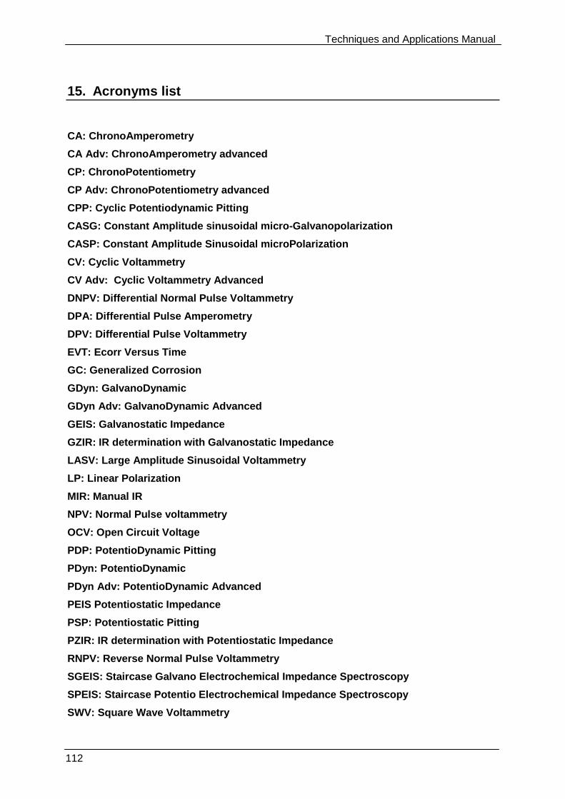
Techniques and Applications Manual
112
15. Acronyms list
CA: ChronoAmperometry
CA Adv: ChronoAmperometry advanced
CP: ChronoPotentiometry
CP Adv: ChronoPotentiometry advanced
CPP: Cyclic Potentiodynamic Pitting
CASG: Constant Amplitude sinusoidal micro-Galvanopolarization
CASP: Constant Amplitude Sinusoidal microPolarization
CV: Cyclic Voltammetry
CV Adv: Cyclic Voltammetry Advanced
DNPV: Differential Normal Pulse Voltammetry
DPA: Differential Pulse Amperometry
DPV: Differential Pulse Voltammetry
EVT: Ecorr Versus Time
GC: Generalized Corrosion
GDyn: GalvanoDynamic
GDyn Adv: GalvanoDynamic Advanced
GEIS: Galvanostatic Impedance
GZIR: IR determination with Galvanostatic Impedance
LASV: Large Amplitude Sinusoidal Voltammetry
LP: Linear Polarization
MIR: Manual IR
NPV: Normal Pulse voltammetry
OCV: Open Circuit Voltage
PDP: PotentioDynamic Pitting
PDyn: PotentioDynamic
PDyn Adv: PotentioDynamic Advanced
PEIS Potentiostatic Impedance
PSP: Potentiostatic Pitting
PZIR: IR determination with Potentiostatic Impedance
RNPV: Reverse Normal Pulse Voltammetry
SGEIS: Staircase Galvano Electrochemical Impedance Spectroscopy
SPEIS: Staircase Potentio Electrochemical Impedance Spectroscopy
SWV: Square Wave Voltammetry

Techniques and Applications Manual
113
TI: Trigger In
TO: Trigger Out
TOS: Trigger Set
VASP: Variable Amplitude Sinusoidal micro Polarization
ZRA: Zero Resistance Ammeter
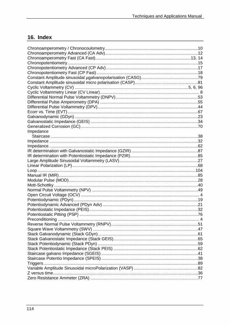
Techniques and Applications Manual
114
16. Index
Chronoamperometry / Chronocoulometry .............................................................................10 Chronoamperometry Advanced (CA Adv).............................................................................12 Chronoamperometry Fast (CA Fast) ............................................................................... 13, 14 Chronopotentiometry ............................................................................................................15 Chronopotentiometry Advanced (CP Adv) ............................................................................17 Chronopotentiometry Fast (CP Fast) ....................................................................................18 Constant Amplitude sinusoidal µgalvanopolarisation (CASG) ...............................................79 Constant Amplitude sinusoidal micro polarisation (CASP) ....................................................81 Cyclic Voltammetry (CV) .............................................................................................. 5, 6, 96 Cyclic Voltammetry Linear (CV Linear) .................................................................................. 8 Differential Normal Pulse Voltammetry (DNPV) ....................................................................53 Differential Pulse Amperometry (DPA) .................................................................................55 Differential Pulse Voltammetry (DPV) ...................................................................................44 Ecorr vs. Time (EVT) ............................................................................................................67 Galvanodynamic (GDyn) ......................................................................................................23 Galvanostatic Impedance (GEIS) .........................................................................................34 Generalized Corrosion (GC) .................................................................................................70 Impedance
Staircase ..........................................................................................................................38 Impedance ...........................................................................................................................32 Impedance ...........................................................................................................................62 IR determination with Galvanostatic Impedance (GZIR) .......................................................87 IR determination with Potentiostatic Impedance (PZIR) ........................................................85 Large Amplitude Sinusoidal Voltammetry (LASV) .................................................................27 Linear Polarization (LP) ........................................................................................................68 Loop ................................................................................................................................... 104 Manual IR (MIR) ...................................................................................................................85 Modular Pulse (MOD) ...........................................................................................................28 Mott-Schottky .......................................................................................................................40 Normal Pulse Voltammetry (NPV) ........................................................................................49 Open Circuit Voltage (OCV) .................................................................................................. 4 Potentiodynamic (PDyn) .......................................................................................................19 Potentiodynamic Advanced (PDyn Adv) ...............................................................................21 Potentiostatic Impedance (PEIS) ..........................................................................................32 Potentiostatic Pitting (PSP) ..................................................................................................76 Preconditioning ..................................................................................................................... 4 Reverse Normal Pulse Voltammetry (RNPV) ........................................................................51 Square Wave Voltammetry (SWV) .......................................................................................47 Stack Galvanodynamic (Stack GDyn) ...................................................................................61 Stack Galvanostatic Impedance (Stack GEIS) ......................................................................65 Stack Potentiodynamic (Stack PDyn) ...................................................................................59 Stack Potentiostatic Impedance (Stack PEIS) ......................................................................62 Staircase galvano Impedance (SGEIS) ................................................................................41 Staircase Potentio Impedance (SPEIS) ................................................................................38 Triggers ................................................................................................................................89 Variable Amplitude Sinusoidal microPolarization (VASP) .....................................................82 Z versus time ........................................................................................................................36 Zero Resistance Ammeter (ZRA) .........................................................................................77


![K EC, KVKE EC, TFSR EC, TFSK EC, KVO EC, KD EC · k ec, kvke ec, tfsr ec, tfsk ec, kvo ec, kd ec ... sk si gb fr ... 1=min 5 (10,0v) 0 0.5 1 1.5 2 0 200 400 600 [m³/s] [pa]](https://img.pdfslide.us/doc/110x75/5ad4f62a7f8b9a571e8ce97b/k-ec-kvke-ec-tfsr-ec-tfsk-ec-kvo-ec-kd-ec-ec-kvke-ec-tfsr-ec-tfsk-ec-kvo.jpg)