Embed Size (px)
Citation preview
Dynamical Systems Model of the Simple Genetic Algorithm
Introduction to Michael Vose’s Theory
Rafal [email protected]
Summer Lecture Series 2002
08/29Summer Lecture Series
2002 2
Overview
Introduction to Vose's ModelDefining Mixing MatricesFinite PopulationsConclusions

08/29Summer Lecture Series
2002 3
OverviewIntroduction to Vose's Model
SGA as a Dynamical SystemRepresenting PopulationsRandom Heuristic SearchInterpretations and Properties
of G(x)Modeling Proportional Selection
Defining Mixing MatricesFinite PopulationsConclusions
08/29Summer Lecture Series
2002 4
OverviewIntroduction to Vose's ModelDefining Mixing Matrices
What is Mixing?Modeling MutationModeling RecombinationProperties of Mixing
Finite PopulationsConclusions
08/29Summer Lecture Series
2002 5
OverviewIntroduction to Vose's ModelDefining Mixing MatricesFinite Populations
Fixed-PointsMarkov ChainMetastable States
Conclusions

08/29Summer Lecture Series
2002 6
OverviewIntroduction to Vose's ModelDefining Mixing MatricesFinite PopulationsConclusions
Properties and Conjectures of G(x)Summary
08/29Summer Lecture Series
2002 7
OverviewIntroduction to Vose's Model
SGA as a Dynamical SystemRepresenting PopulationsRandom Heuristic SearchInterpretations and Properties
of G(x)Modeling Proportional Selection
Defining Mixing MatricesFinite PopulationsConclusions

08/29Summer Lecture Series
2002 8
Introduction to Vose's Dynamical Systems Model
SGA as a Dynamical System
What is a dynamical system?
→ a set of possible states, together with a rule that determines the present state in terms of past states.
When a dynamical system is deterministic?
→ If the present state can be determined uniquely from the past states (no randomness is allowed).

08/29Summer Lecture Series
2002 9
Introduction to Vose's Dynamical Systems Model
SGA as a Dynamical System
1. SGA usually starts with a random population.
2. One generation later we will have a new population.
3. Because the genetic operators have a random element, we cannot say exactly what the next population will be (algorithm is not deterministic!!!).

08/29Summer Lecture Series
2002 10
Introduction to Vose's Dynamical Systems Model
SGA as a Dynamical SystemHowever, we can calculate:→ the probability distribution over
the set of possible populations defined by the genetic operators
→ expected next population
As the population size tends to infinity:
→ the probability that the next population will be the expected one tends to 1 (algorithm becomes deterministic)
→ and the trajectory of expected next population gives the actual behavior.
08/29Summer Lecture Series
2002 11
Introduction to Vose's Dynamical Systems Model
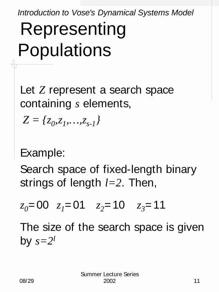
Representing Populations
Let Z represent a search space containing s elements, Z = {z0,z1,…,zs-1}
Example:Search space of fixed-length binary strings of length l=2. Then,
z0=00 z1=01 z2=10 z3=11
The size of the search space is given by s=2l
08/29Summer Lecture Series
2002 12
Introduction to Vose's Dynamical Systems Model
Representing Populations
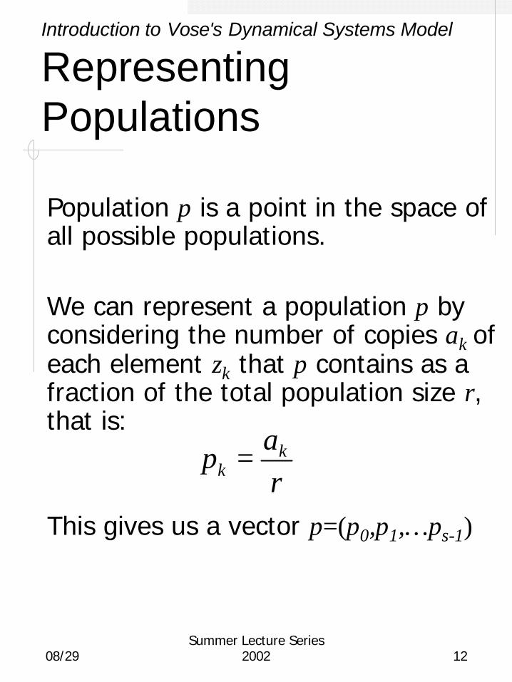
Population p is a point in the space of all possible populations.
We can represent a population p by considering the number of copies ak of each element zk that p contains as a fraction of the total population size r, that is:
This gives us a vector p=(p0,p1,…ps-1)
ra
p kk =
08/29Summer Lecture Series
2002 13
Introduction to Vose's Dynamical Systems Model
Representing Populations
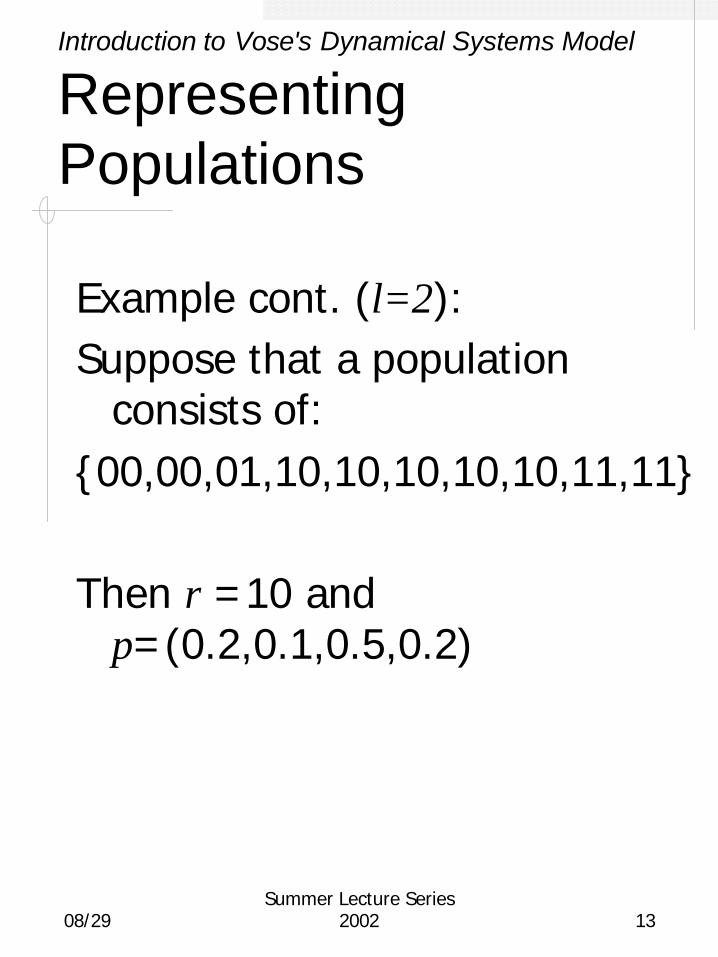
Example cont. (l=2):Suppose that a population
consists of:{00,00,01,10,10,10,10,10,11,11}
Then r =10 and p=(0.2,0.1,0.5,0.2)

08/29Summer Lecture Series
2002 14
Introduction to Vose's Dynamical Systems Model
Representing PopulationsProperties of population vectors:
1. p is an element of the vector space Rs (addition and/or multiplication by scalar produce other vectors within Rs)
2. Each entry pk must lie in the range [0,1]
3. All entries of p sum to 1
The set of all vectors in Rs that satisfy these properties is called the simplex and denoted by Λ.

08/29Summer Lecture Series
2002 15
Introduction to Vose's Dynamical Systems Model
Representing PopulationsExamples of Simplex Structures:1. The simplest case:
Search space has only two elementsZ = {z0,z1}
Population vectors are contained in R2
Simplex Λ is a segment of a straight line:
08/29Summer Lecture Series
2002 16
Introduction to Vose's Dynamical Systems Model
Representing Populations
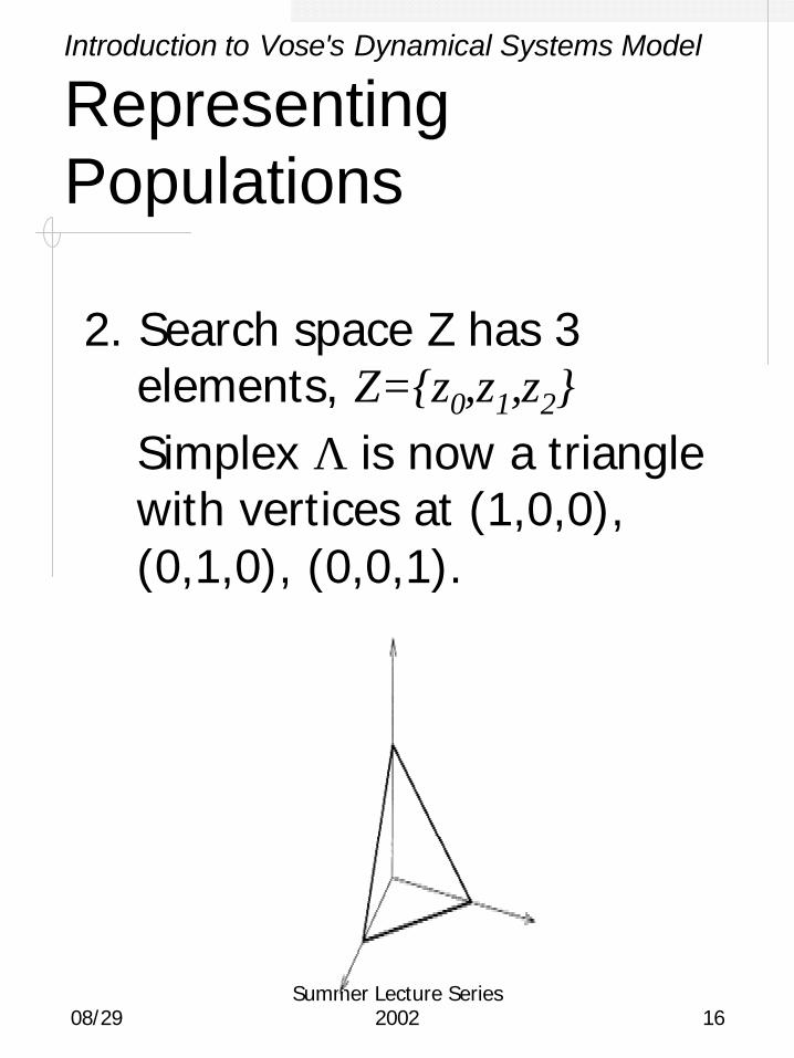
2. Search space Z has 3 elements, Z={z0,z1,z2}Simplex Λ is now a trianglewith vertices at (1,0,0), (0,1,0), (0,0,1).

08/29Summer Lecture Series
2002 17
Introduction to Vose's Dynamical Systems Model
Representing Populations
In general, in s dimensional space the simplex forms (s-1)-dimensional object (a hyper-tetrahedron).The vertices of the simplex correspond to populations with copies of only one element.

08/29Summer Lecture Series
2002 18
Introduction to Vose's Dynamical Systems Model
Representing Populations
Properties of the Simplex:→ Set of possible populations of a
given size r takes up a finitesubset of the simplex.
→ Thus, the simplex contains some vectors that could never be real populations because they have irrational entries.
→ But, as the population size rtends to infinity, the set of possible populations becomes dense in the simplex.
08/29Summer Lecture Series
2002 19
Introduction to Vose's Dynamical Systems Model
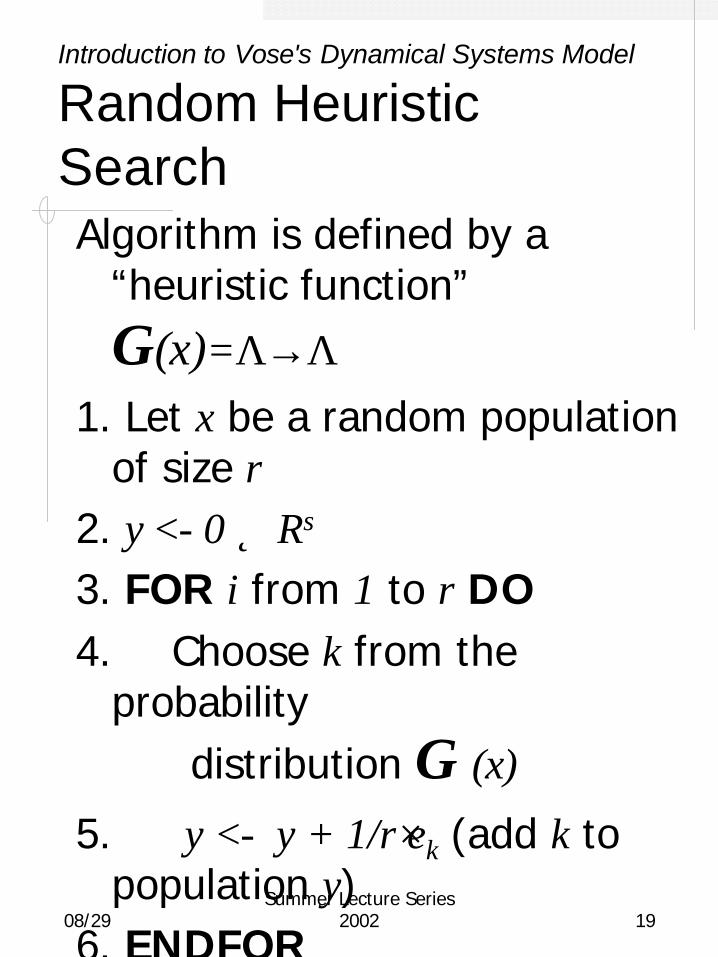
Random Heuristic SearchAlgorithm is defined by a
“heuristic function”
G(x)=Λ→Λ
1. Let x be a random population of size r
2. y <- 0 ∈ Rs
3. FOR i from 1 to r DO4. Choose k from the
probability distribution G (x)
5. y <- y + 1/r⋅ek (add k to population y)
6. ENDFOR

08/29Summer Lecture Series
2002 20
Introduction to Vose's Dynamical Systems Model
Interpretations of G(x)
1. G(x) is the expected next generation population
2. G(x) is the limiting next population as the population size goes to infinity
3. G(x)j is the probability that j∈Zis selected to be in the next generation

08/29Summer Lecture Series
2002 21
Introduction to Vose's Dynamical Systems Model
Properties of G(x)
G(x) = U(C(F(x))), where F describes selection, U describes
mutation, and C describes recombination.
x ->G(x) is a discrete-time dynamical system

08/29Summer Lecture Series
2002 22
Introduction to Vose's Dynamical Systems Model
Simple Genetic Algorithm
1. Let X be a random population of size r.
2. To generate a new population Y do the following r times:- choose two parents from X with probability in proportion to fitness- apply crossover to parents to obtain a child individual - apply mutation to the child- add the child to new population y
3. Replace X by Y4. Go to step 2.

08/29Summer Lecture Series
2002 23
Introduction to Vose's Dynamical Systems Model
Modeling Proportional Selection
Let p=(p0,p1,…ps-1) be our current population.We want to calculate the probability that zk will be selected for the next population.Using fitness proportional selection, we know this probability is equal to:
)()(pf
pzf kk ⋅

08/29Summer Lecture Series
2002 24
Introduction to Vose's Dynamical Systems Model
Modeling Proportional Selection
The average fitness of the population p can be calculated by:
We can create a new vector q, where qk equals the probability that zk is selected.We can think of q as a result of applying an operator F to p, that is q = F p
∑−
=
⋅=1
0
)()(s
kkk pzfpf
08/29Summer Lecture Series
2002 25
Introduction to Vose's Dynamical Systems Model
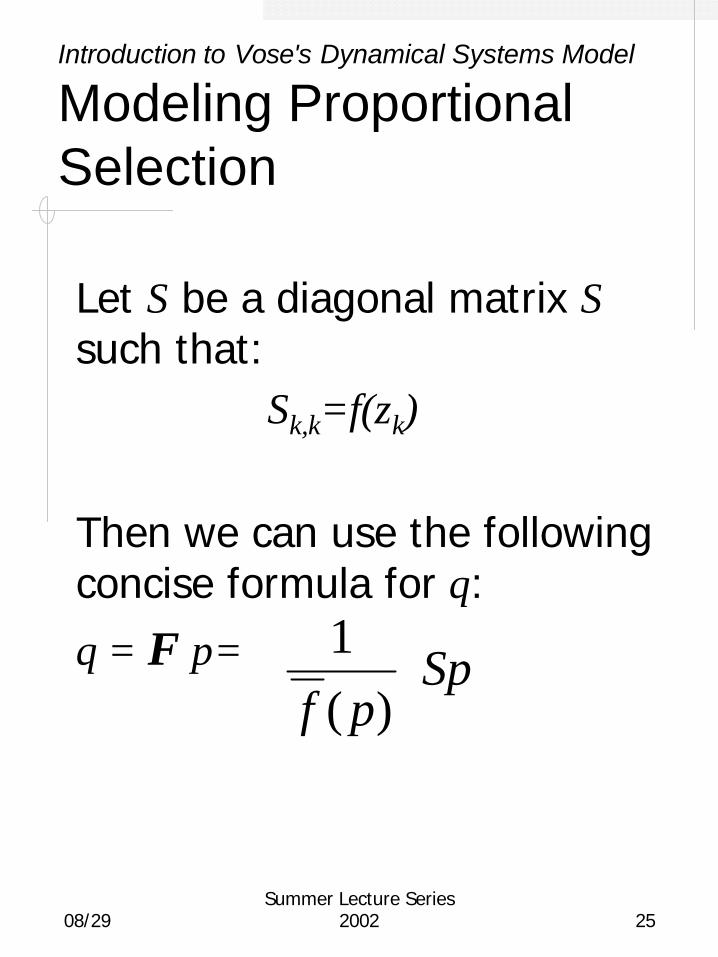
Modeling Proportional Selection
Let S be a diagonal matrix Ssuch that:
Sk,k=f(zk)
Then we can use the following concise formula for q:
q = F p= Sppf
⋅)(
1

08/29Summer Lecture Series
2002 26
Introduction to Vose's Dynamical Systems Model
Modeling Proportional Selection
Probabilities in q define the probability distribution for the next population, if only selection is applied.
This distribution specified by the probabilities q0,…,qs-1 is a multinomial distribution.

08/29Summer Lecture Series
2002 27
Introduction to Vose's Dynamical Systems Model
Modeling Proportional Selection
Example:Let Z={0,1,2}Let f=(3,1,5)T
Let p=(¼ ,½ ,¼ )T
f(p)=3⋅¼+1⋅½+5⋅¼= 5/2
q = F p=
G
=
⋅=⋅
2151
103
412141
500010003
251
)(1
Sppf
08/29Summer Lecture Series
2002 28
Introduction to Vose's Dynamical Systems Model
Modeling Proportional Selection
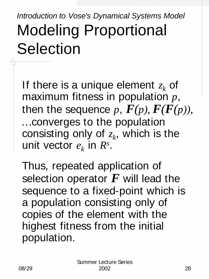
If there is a unique element zk of maximum fitness in population p, then the sequence p, F(p), F(F(p)), …converges to the population consisting only of zk, which is the unit vector ek in Rs.
Thus, repeated application of selection operator F will lead the sequence to a fixed-point which is a population consisting only of copies of the element with the highest fitness from the initial population.
08/29Summer Lecture Series
2002 29
OverviewIntroduction to Vose's ModelDefining Mixing Matrices
What is Mixing?Modeling MutationModeling RecombinationProperties of Mixing
Finite PopulationsConclusions
08/29Summer Lecture Series
2002 30
Defining Mixing Matrices
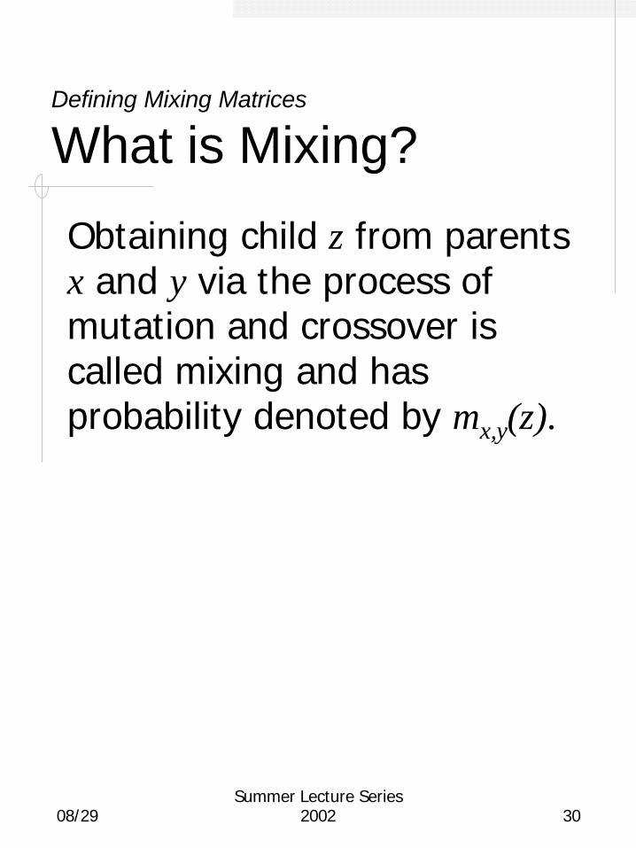
What is Mixing?
Obtaining child z from parents x and y via the process of mutation and crossover is called mixing and has probability denoted by mx,y(z).

08/29Summer Lecture Series
2002 31
Defining Mixing Matrices
Modeling MutationWe want to know the probability that after mutating individuals that have been selected, we end up with a particular individual.
There are two ways to obtain copies of zi after mutation:- other individual zj is selected and mutated to
produce zi
- zi is selected itself and not mutated

08/29Summer Lecture Series
2002 32
Defining Mixing Matrices
Modeling Mutation
The probability of ending up with ziafter selection and mutation is:
where Ui,j is the probability that zjmutates to form zi
Example:The probability of mutating z5=101 to z0=000 is equal to:U0,5=µ2(1- µ)
j
s
jji qU∑
−
=
1
0,

08/29Summer Lecture Series
2002 33
Defining Mixing Matrices
Modeling Mutation
We can put all the Ui,jprobabilities in the matrix U. For example, in case of l=2 we obtain:

08/29Summer Lecture Series
2002 34
Defining Mixing Matrices
Modeling Mutation
If p is a population, then (Up)jis the probability that individual j results from applying only mutation to p.
With a positive mutation rate less than 1, the sequence p, U(x), U(U(x)), … converges to the population with all elements of Z represented equally (the center of the simplex).
08/29Summer Lecture Series
2002 35
Defining Mixing Matrices
Modeling Mutation
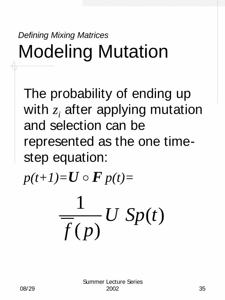
The probability of ending up with zi after applying mutation and selection can be represented as the one time-step equation:p(t+1)=U é F p(t)=
1( )
( )U Sp t
f p

08/29Summer Lecture Series
2002 36
Defining Mixing Matrices
Modeling Mutation
Will this sequence converge as time goes to infinity?This sequence will converge to a fixed-point p satisfying:U S p = f(p) pThis equation states that the fixed-point population p is an eigenvectorof the matrix U S and that the average fitness of p is the corresponding eigenvalue.

08/29Summer Lecture Series
2002 37
Defining Mixing Matrices
Modeling Mutation
Perron-Frobenius Theorem (for matrices with positive real entries)
From this theorem we know that U S will have exactly one eigenvector in the simplex, and that this eigenvector corresponds to the leading eigenvalue (the one with the largest absolute value).

08/29Summer Lecture Series
2002 38
Defining Mixing Matrices
Modeling MutationSummarizing, for SGA under
proportional selection and bitwise mutation:
1. Fixed-points are eigenvectors of US, once they have been scaled so that their components sum to 1.
2. Eigenvalues of US give the average fitness of the corresponding fixed-point populations.
3. Exactly one eigenvector of US is in the simplex Λ.
4. This eigenvector corresponds to the leading eigenvalue.

08/29Summer Lecture Series
2002 39
Defining Mixing Matrices
Modeling Recombination
Effects of applying crossover can be represented as an operator C acting upon simplex Λ.
(C p)k gives the probability of producing individual zk in the next generation by applying crossover.
08/29Summer Lecture Series
2002 40
Defining Mixing Matrices
Modeling Recombination
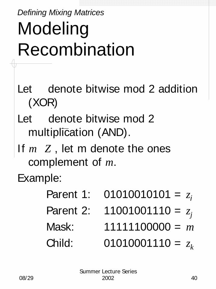
Let ⊕ denote bitwise mod 2 addition (XOR)
Let ⊗ denote bitwise mod 2 multiplication (AND).
If m∈Z , let m denote the ones complement of m.
Example:Parent 1: 01010010101 = zi
Parent 2: 11001001110 = zj
Mask: 11111100000 = mChild: 01010001110 = zk
08/29Summer Lecture Series
2002 41
Defining Mixing Matrices
Modeling Recombination
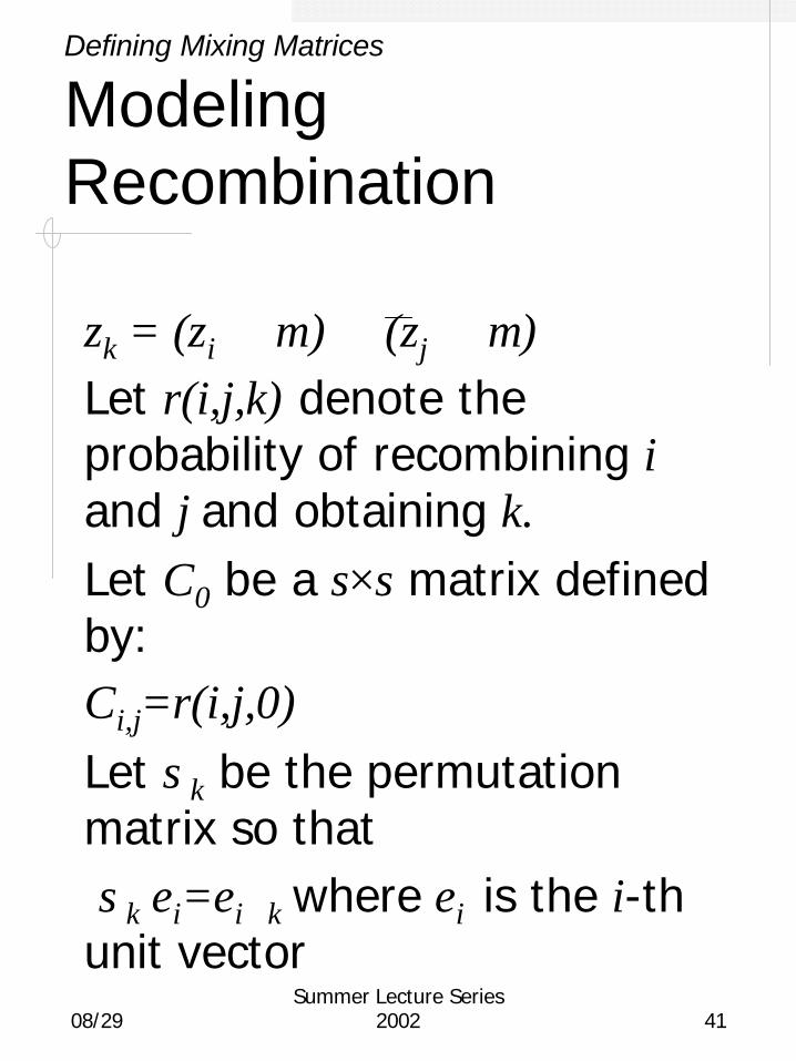
zk = (zi ⊗ m) ⊕ (zj ⊗ m)Let r(i,j,k) denote the probability of recombining iand j and obtaining k.Let C0 be a s×s matrix defined by:Ci,j=r(i,j,0)Let σk be the permutation matrix so thatσk ei=ei⊕k where ei is the i-thunit vector

08/29Summer Lecture Series
2002 42
Defining Mixing Matrices
Modeling Recombination
Define C: Λ→ Λ by
C(p) = (σk p)TC0(σk p)
Then C defines the effect of recombination on a population p.

08/29Summer Lecture Series
2002 43
Defining Mixing Matrices
Modeling Recombination
Example (from Wright):l=2 binary stringsString Fitness00 301 110 211 4

08/29Summer Lecture Series
2002 44
Defining Mixing Matrices
Modeling Recombination
Assume an initial population vector of p=(¼, ¼, ¼, ¼)T
q= F(p)=
Assume one-point crossover with crossover rate of ½
C0 =
08/29Summer Lecture Series
2002 45
Defining Mixing Matrices
Modeling Recombination
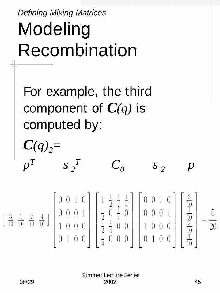
For example, the third component of C(q) is computed by:
C(q)2=pT σ2
T C0 σ2 p
08/29Summer Lecture Series
2002 46
Defining Mixing Matrices
Modeling Recombination
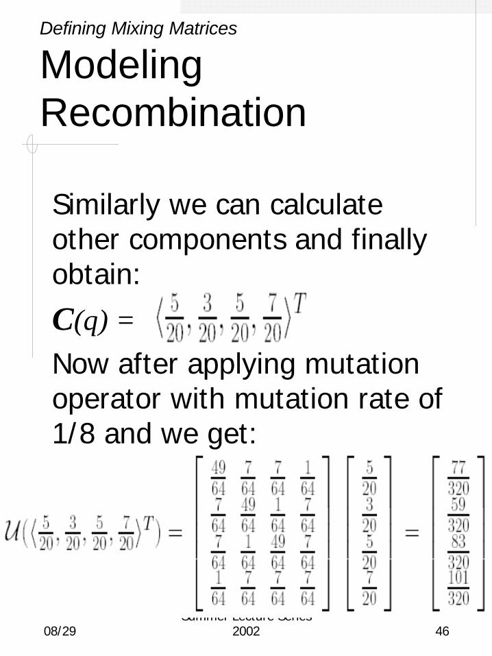
Similarly we can calculate other components and finally obtain:
C(q) = Now after applying mutation operator with mutation rate of 1/8 and we get:
08/29Summer Lecture Series
2002 47
Defining Mixing Matrices
Properties of Mixing
For all the usual kinds of crossover that are used in GAs, the order of crossover and mutation doesn’t matter.
U é C = C é UThe probability of creating a particular individual is the same.

08/29Summer Lecture Series
2002 48
Defining Mixing Matrices
Properties of Mixing
This combination of crossover and mutation (in either order) gives the mixing scheme for the GA, denoted by M.
M = U é C = C é U
The k-th component of M p is:
M(p)k= C(U p)k=(U p)T·(Ck U p)
08/29Summer Lecture Series
2002 49
Defining Mixing Matrices
Properties of Mixing
Let us define Mk=U Ck UThe (i,j)th entry of Mk is the probability that zi and zj, after being mutated and recombined, produce zk.Then the mixing scheme is given by:
M(p)k= pT·(Mk p)= (σk p)T·(M0 σk p)All the information about mutating and recombining is held in the matrix M0 called the mixing matrix.
08/29Summer Lecture Series
2002 50
OverviewIntroduction to Vose's ModelDefining Mixing MatricesFinite Populations
Fixed-PointsMarkov ChainMetastable States
Conclusions
08/29Summer Lecture Series
2002 51
Finite Populations
Fixed-Points
If the population size r is finite, then each component pi of a population vector p must be a rational number with r as a denominator.
The set of possible finite populations of size r forms a discrete lattice within the simplex Λ.

08/29Summer Lecture Series
2002 52
Finite Populations
Fixed-Points
Consequence:Fixed-point population
described by the infinite population model might not actually exist as a possible
population!!!

08/29Summer Lecture Series
2002 53
Finite Populations
Markov Chain
Given an actual (finite) population represented by the vector p(t), we have a probability distribution over all possible next populations defined by G(p)=p(t+1).
The probability of getting a particular population depends only on the previous generation → Markov Chain.

08/29Summer Lecture Series
2002 54
Finite Populations
Markov Chain
A Markov Chain is described by its transition matrix Q.
Qq,p is the probability of going from population p to population q.
∏−
=
=1
0, )!(
))((!
s
j j
rqj
pq rq
pGrQ
j
08/29Summer Lecture Series
2002 55
Finite Populations
Markov Chain
→ p(t+1) itself might not be an actual population
→ p(t+1) is the expected next population
→ Can think of the probability distribution clustered aroundthat population
→ Populations that are close to it in the simplex will be more likely to occur as a next population than the ones that are far away

08/29Summer Lecture Series
2002 56
Finite Populations
Markov Chain
→ A good way to visualize this is to think of the operator G as defining an arrow at each point in the simplex
→ At a fixed-point of G, the arrow has 0 length
→ Thus, SGA is likely to spend much of its time at populations that are in the vicinity of the infinite population fixed-point
08/29Summer Lecture Series
2002 57
Finite Populations
Metastable States
Metastable states are parts of the simplex where the force of G is small, even if these areas are not near the fixed-point.
They are important in understanding the long-term behavior of a finite populationGA.
08/29Summer Lecture Series
2002 58
Finite Populations
Metastable States
We extend G to apply to the whole of Rs.
Perron-Frobenius theory predicts only one fixed-point in the simplex, but we are now considering the action of G on the whole of Rs.
If there are other fixed-point close to the simplex, then by continuity of G, there will be a metastableregion in that part of the simplex.
08/29Summer Lecture Series
2002 59
Finite Populations
Metastable States
Metastable states are simply other eigenvectors of U S suitably scaled so that their components sum to one.
To find potential metastablestates within the simplex, we simply calculate all the eigenvectors of US
08/29Summer Lecture Series
2002 60
OverviewIntroduction to Vose's ModelDefining Mixing MatricesFinite PopulationsConclusions
Properties and Conjectures of G(x)Summary
08/29Summer Lecture Series
2002 61
Conclusions
Properties and Conjectures of G(x)
The principle conjecture:G is focused under reasonable assumptions about crossover and mutation
→ Known to be true if mutation is defined bitwise with a mutation rate <0.5 and there is no crossover.
→ When there is crossover it is known to be true when the fitness function is linear (or near to linear) and the mutation rate is small.
08/29Summer Lecture Series
2002 62
Conclusions
Properties and Conjectures of G(x)
The second conjecture:Fixed points of G are hyperbolicfor nearly all fitness functions
→ Important for determining the stability of fixed points
→ Known to be true for the case of fixed-length binary strings, proportional selection, any kind of crossover, and mutation defined bitwise with a positive mutation rate

08/29Summer Lecture Series
2002 63
Conclusions
Properties and Conjectures of G (x)
The third conjecture:G is well-behaved
→ Known to be true if the mutation rate is positive but < 0.5 and if crossover is applied at a rate that is less than 1.

08/29Summer Lecture Series
2002 64
Conclusions
Properties and Conjectures of G(x)
Assuming all three conjectures are true, then the following properties follow:
1. There are only finitely many fixed-points of G.
2. The probability of picking a population p, such that iterates of G applied to p converge on an unstable fixed-point in zero.
3. The infinite population GA converges to a fixed-point in logarithmic time.
08/29Summer Lecture Series
2002 65
Conclusions
Summary
Michael Vose’s theory of the SGA:→ Gives a general mathematical
framework for the analysis of the SGA
→ Uses dynamical systems models to predict the actual behavior (trajectory) of the SGA
→ Provides results that are general in nature, but also applicable to real situations
→ Lays some theoretical foundations toward building the GA theory

08/29Summer Lecture Series
2002 66
Conclusions
Summary
But…→ Is intractable in all except
for the simple cases→ Approximations are
necessary to the Vose SGA model to make it tractable in real situations
08/29Summer Lecture Series
2002 67
OverviewIntroduction to Vose's ModelDefining Mixing MatricesFinite PopulationsConclusions


![[PPT]Genetic Algorithms - Computer Sciencedinitz/Course/SS-12/Genetic... · Web viewOutline Evolution in the nature Genetic Algorithms and Genetic Programming A simple example for](https://img.pdfslide.us/doc/110x75/5b07c15e7f8b9a56408d8305/pptgenetic-algorithms-computer-science-dinitzcoursess-12geneticweb-viewoutline.jpg)