e FINAL REPORT ON NASA GRANT NAG 3-634 · final report on nasa grant nag 3-634 e “comparison of unl laser imaging and sizing system and a phase/doppler system for analyzing sprays

e FINAL REPORT ON NASA GRANT NAG 3-634

e

“COMPARISON OF UNL LASER IMAGING AND SIZING SYSTEM AND A PHASE/DOPPLER SYSTEM FOR ANALYZING

SPRAYS FROM A NASA NOZZLE” e

(Grant period: April 1, 1985 to August 19, 1987)

e

e

e

e

From

( b A S A - C R - 1 8 2 4 3 7 ) CCMFIfrISCb CF UIL L A S E 3 M88- 16456 1 L B G I h G AND SIZING SYZ’IEH BNZ: A EBASE/CCFELEE SYSIEB ECB A b ’ B 1 Y Z I h ; G SPRAYS PHCH A E A S A NCZPLE € i n a l R e f . G r t , 1 Apr- 1985 Unclas - 19 Bug, 1967 (hr lraska uciv,) 139 p G3/3& 0121954

Dennis R. Alexander Laboratory for Elect ro-0 pt ical Measurements

Department of Mechanical Engineering Room 255 WSEC

University of Nebraska-Lincoln Lincoln, NE 68588-0525

e

https://ntrs.nasa.gov/search.jsp?R=19880007572 2020-03-26T23:37:24+00:00Z

e

ABSTRACT

0

e

0

Research was conducted on aerosol spray characterization using a P/DPA and a laser imag-

ing/video processing system on a NASA MOD-1 air-assist nozzle being evaluated for use in aircraft

icing research. Benchmark tests were performed on monodispersed particles and on the NASA

MOD-1 nozzle under identical laboratory operating conditions. The laser imaging/video process-

ing system and the P/DPA showed agreement on calibration tests in monodispersed aerosol sprays

o f f 2.6 pm with a standard deviation off 2.6 pm. Benchmark tests were performed on the NASA

MOD-1 nozzle on the centerline and radially at one-half inch increments to the outer edge of the

spray plume at a distance 2 feet (0.61 m) downstream from the exit of the nozzle. Comparative

results at two operating conditions of the nozzle are presented for the two instruments. For the first

case studied, the deviation in arithmetic mean diameters determined by the two instruments was

in a range of 0.1 to 2.8 pm, and the deviation in Sauter mean diameters varied from 0 to 2.2 pm.

Operating conditions in the second case were more severe which resulted in the arithmetic mean

diameter deviating from 1.4 to 7.1 pm and the deviation in the Sauter mean diameters ranging

from 0.4 to 6.7 pm.

0

0

a

Contents

1 I N T R O D U C T I O N 1

2 EXPERIMENTAL APPARATUS AND P R O C E D U R E 3 2.1 P / D P A . . . . . . . . . . . . . . . . . . . . . . . . . . . . . . . . . . . . . . . . . . 3 2.2 Laser Imaging/Video Processing System . . . . . . . . . . . . . . . . . . . . 7

2.2.1 Components . . . . . . . . . . . . . . . . . . . . . . . . . . . . . . . . . . . . 7 2.2.2 Sizing Method: Segmentation . . . . . . . . . . . . . . . . . . . . . . . . . . 11 2.2.3 Calibration . . . . . . . . . . . . . . . . . . . . . . . . . . . . . . . . . . . . 13 2.2.4 Focus Method . . . . . . . . . . . . . . . . . . . . . . . . . . . . . . . . . . . . 15 2.2.5 Modifications . . . . . . . . . . . . . . . . . . . . . . . . . . . . . . . . . . . 20 2.2.6 Software Updates . . . . . . . . . . . . . . . . . . . . . . . . . . . . . . . . . 22

2.3 Spray Test Facility . . . . . . . . . . . . . . . . . . . . . . . . . . . . . . . . . . 22 2.3.1 MOD-1Nozzle . . . . . . . . . . . . . . . . . . . . . . . . . . . . . . . . . . 29 2.3.2 Air and Water Supply System (AWSS) . . . . . . . . . . . . . . . . . . . . . 29 2.3.3 Water Flowmeter Calibration . . . . . . . . . . . . . . . . . . . . . . . . . . 29

2.4 Digital Pressure Acquisition . . . . . . . . . . . . . . . . . . . . . . . . . . . . 29 2.4.1 Pressure Transducers . . . . . . . . . . . . . . . . . . . . . . . . . . . . . . . 32 2.4.2 A/D converter board . . . . . . . . . . . . . . . . . . . . . . . . . . . . . . . 32 2.4.3 Analog-to-Digit al Conversion . . . . . . . . . . . . . . . . . . . . . . . . . . 32 2.4.4 Digital Pressure System Calibration . . . . . . . . . . . . . . . . . . . . . . 32

2.5 Experimental Procedure . . . . . . . . . . . . . . . . . . . . . . . . . . . . . . . 32 2.5.1 Verification Tests . . . . . . . . . . . . . . . . . . . . . . . . . . . . . . . . . 35 2.5.2 Spray Comparison . . . . . . . . . . . . . . . . . . . . . . . . . . . . . . . . 38

e

3 PRESENTATION AND DISCUSSION O F RESULTS 39 3.1 LI /VPS Calibration Results 39 3.2 Results For t h e MOD-1 Nozzle Comparison . . . . . . . . . . . . . . . . . . 47

3.2.1 Discussion of Results for Comparison . CASE I . . . . . . . . . . . . . . . . 86 3.2.2 Discussion of Results for Comparison . CASE I1 . . . . . . . . . . . . . . . 86

0 . . . . . . . . . . . . . . . . . . . . . . . . . . . .

0 4 CONCLUSIONS A N D RECOMMENDATIONS 93 4.1 LI /VPS . . . . . . . . . . . . . . . . . . . . . . . . . . . . . . . . . . . . . . . . . 93 4.2 LI/VPSandP/DPAComparison . . . . . . . . . . . . . . . . . . . . . . . . . 93 4.3 Suggestions and Recommendation for Future Work . . . . . . . . . . . . . 94

5 R E F E R E N C E S 96 e 6 A P P E N D I X A: E Q U I P M E N T LISTING 98

1

a

a

e

7 APPENDIX B Design and Implementation of the PSP Laser Trigger

8 APPENDIX C.l: PSP Set-up Program

9 APPENDIX C.2: PSP Graphical Presentation of Results

10 APPENDIX C.3: MOD-1 Nozzle Input Pressure Determination

11 APPENDIX C.4: PSP Magnification Correction Factor Determination

12 APPENDIX D: Mean Diameter Calculations

13 APPENDIX E: Cole-Palmer Flowmeter Calibration Data

14 APPENDIX F: OMEGA Pressure Transducer Calibration Data

100

103

114

122

124

126

127

129

0

a

0

a

e

.. 11

a

e

0

List of Figures

e

2.1 Phase Doppler/Particle Analyzer . . . . . . . . . . . . . . . . . . . . . . . . . . . . 4 2.2 P/DPAPMTSignals . . . . . . . . . . . . . . . . . . . . . . . . . . . . . . . . . . . 5 2.3 P/DPA Setup Page . . . . . . . . . . . . . . . . . . . . . . . . . . . . . . . . . . . . 6 . 2.4 Reflections Caused by High Density Spray . . . . . . . . . . . . . . . . . . . . . . . 8 2.5 Drop Distribution Behavior with increasing PMT Voltage . . . . . . . . . . . . . . 8 2.6 LI/VPS Laser Imaging Device . . . . . . . . . . . . . . . . . . . . . . . . . . . . . . 9 2.7 LI/VPS Video Processor Schematic . . . . . . . . . . . . . . . . . . . . . . . . . . . 10 2.8 LI/VPS Particle Representation . . . . . . . . . . . . . . . . . . . . . . . . . . . . . 12 2.9 Two-Dimensional Calibration Technique . . . . . . . . . . . . . . . . . . . . . . . . 14 2.10 Calibration Reticle . . . . . . . . . . . . . . . . . . . . . . . . . . . . . . . . . . . . 16 2.11 Flow Diagram for Calibration Procedure . . . . . . . . . . . . . . . . . . . . . . . . 18 2.12 LI/VPS Focus . . . . . . . . . . . . . . . . . . . . . . . . . . . . . . . . . . . . . . . 19 2.13 Static vs . Dynamic Particle Representation in CPM . . . . . . . . . . . . . . . . . 21 2.14 Comparison of the MAGL Parameter for Dynamic and Stationary Particles in CPM 23 2.15 Flow Diagram for the Particle Sizing Program in SPM . . . . . . . . . . . . . . . . 24 2.16 Comparison of the MAGL Parameter for SPM and CPM . . . . . . . . . . . . . . . 25 2.17 PSP Setup Page . . . . . . . . . . . . . . . . . . . . . . . . . . . . . . . . . . . . . 26 2.18 PSP Graphic Package . . . . . . . . . . . . . . . . . . . . . . . . . . . . . . . . . . 27 2.19 Equipment Schematic for Instrument Comparison . . . . . . . . . . . . . . . . . . . 28 2.20 MOD-1 Nozzle . . . . . . . . . . . . . . . . . . . . . . . . . . . . . . . . . . . . . . 30 2.21 Air and Water Supply Schematic . . . . . . . . . . . . . . . . . . . . . . . . . . . . 31 2.22 OMEGA Pressure Transducers . . . . . . . . . . . . . . . . . . . . . . . . . . . . . 33 2.23 A/D Connector Box Schematic . . . . . . . . . . . . . . . . . . . . . . . . . . . . . 34 2.24 P/DPA Doppler Fringes as Seen by the LI/VPS Imaging Camera . . . . . . . . . . 36 2.25 P/DPA and LI/VPS Over-lapping Probe Volumes . . . . . . . . . . . . . . . . . . 36 2.26 Verification Test Apparatus . . . . . . . . . . . . . . . . . . . . . . . . . . . . . . . 37

3.1 Magnification Correction Factor Behavior . . . . . . . . . . . . . . . . . . . . . . . 41 3.2 Magnification Correction Factor Behavior . . . . . . . . . . . . . . . . . . . . . . . 42 3.3 Magnification Correction Factor Behavior . . . . . . . . . . . . . . . . . . . . . . . 43 3.4 Magnification Correction Factor Behavior . . . . . . . . . . . . . . . . . . . . . . . 44 3.5 VOAG Verification w/o Dispersion Cup . . . . . . . . . . . . . . . . . . . . . . . . 49 3.6 VOAG Verification w/o Dispersion Cup . . . . . . . . . . . . . . . . . . . . . . . . 50 3.7 VOAG Verification w/o Dispersion Cup . . . . . . . . . . . . . . . . . . . . . . . . 51 3.8 VOAG Verification w/o Dispersion Cup . . . . . . . . . . . . . . . . . . . . . . . . 52 3.9 VOAG Verification w/o Dispersion Cup . . . . . . . . . . . . . . . . . . . . . . . . 53 3.10 VOAG Verification w/o Dispersion Cup . . . . . . . . . . . . . . . . . . . . . . . . 54 3.11 VOAG Verification w/o Dispersion Cup . . . . . . . . . . . . . . . . . . . . . . . . 55

... 111

e

0

0

0

e

a

0

e

a

3.12 VOAG Verification w/o Dispersion Cup . . . . . . . . . . . . . . . . . . . . . . . . 56 3.13 VOAG Verification w/o Dispersion Cup . . . . . . . . . . . . . . . . . . . . . . . . 57 3.14 VOAG Verification w/ Dispersion Cup . . . . . . . . . . . . . . . . . . . . . . . . . 58 3.15 VOAG Verification w/ Dispersion Cup . . . . . . . . . . . . . . . . . . . . . . . . . 59 3.16 VOAG Verification w/ Dispersion Cup . . . . . . . . . . . . . . . . . . . . . . . . . 60 3.17 VOAG Verification w/ Dispersion Cup . . . . . . . . . . . . . . . . . . . . . . . . . 61 3.18 VOAG Verification w/ Dispersion Cup . . . . . . . . . . . . . . . . . . . . . . . . . 62 3.19 VOAG Verification w/ Dispersion Cup . . . . . . . . . . . . . . . . . . . . . . . . . 63 3.20 VOAG Verification w/ Dispersion Cup . . . . . . . . . . . . . . . . . . . . . . . . . 64 3.21 VOAG Verification w/ Dispersion Cup . . . . . . . . . . . . . . . . . . . . . . . . . 65 3.22 VOAG Verification w/ Dispersion Cup . . . . . . . . . . . . . . . . . . . . . . . . . 66 3.23 Comparison of Arithmetic Mean Diameters for CASE I VOAG Verification w/o

Dispersion Cup Results . . . . . . . . . . . . . . . . . . . . . . . . . . . . . . . . . . 67 3.24 Comparison of Arithmetic Mean Diameters for CASE I1 VOAG Verification w/

Dispersion Cup Results . . . . . . . . . . . . . . . . . . . . . . . . . . . . . . . . . . 68 3.25 MOD-1 Nozzle Comparison . . . . . . . . . . . . . . . . . . . . . . . . . . . . . . . 70 3.26 MOD-1 Nozzle Comparison . . . . . . . . . . . . . . . . . . . . . . . . . . . . . . . 71 3.27 MOD-1 Nozzle Comparison . . . . . . . . . . . . . . . . . . . . . . . . . . . . . . . 72 3.28 MOD-1 Nozzle Comparison . . . . . . . . . . . . . . . . . . . . . . . . . . . . . . . 73 3.29 MOD-1 Nozzle Comparison . . . . . . . . . . . . . . . . . . . . . . . . . . . . . . . 74 3.30 MOD-1 Nozzle Comparison . . . . . . . . . . . . . . . . . . . . . . . . . . . . . . . 75 3.31 MOD-1 Nozzle Comparison . . . . . . . . . . . . . . . . . . . . . . . . . . . . . . . 76 3.32 MOD-1 Nozzle Comparison . . . . . . . . . . . . . . . . . . . . . . . . . . . . . . . 77 3.33 MOD-1 Nozzle Comparison . . . . . . . . . . . . . . . . . . . . . . . . . . . . . . . 78 3.34 MOD-1 Nozzle Comparison . . . . . . . . . . . . . . . . . . . . . . . . . . . . . . . 79 3.35 MOD-1 Nozzle Comparison . . . . . . . . . . . . . . . . . . . . . . . . . . . . . . . 80 3.36 MOD-1 Nozzle Comparison . . . . . . . . . . . . . . . . . . . . . . . . . . . . . . . 81 3.37 MOD-1 Nozzle Comparison . . . . . . . . . . . . . . . . . . . . . . . . . . . . . . . 82 3.38 MOD-1 Nozzle Comparison . . . . . . . . . . . . . . . . . . . . . . . . . . . . . . . 83 3.39 MOD-1 Nozzle Comparison . . . . . . . . . . . . . . . . . . . . . . . . . . . . . . . 84 3.40 MOD-1 Nozzle Comparison . . . . . . . . . . . . . . . . . . . . . . . . . . . . . . . 85 3.41 Comparison of Arithmetic Mean Diameters for MOD-1 Nozzle Comparison Test .

CASE1 . . . . . . . . . . . . . . . . . . . . . . . . . . . . . . . . . . . . . . . . . . . 88 3.42 Comparison of Sauter Mean Diameters for MOD-1 Nozzle Comparison Test . CASE I 89 3.43 Comparison of Arithmetic Mean Diameters for MOD-1 Nozzle Comparison Test .

CASE II . . . . . . . . . . . . . . . . . . . . . . . . . . . . . . . . . . . . . . . . . . . 90 3.44 Comparison of Sauter Mean Diameters for MOD-1 Nozzle Comparison Test . CASE

I1 . . . . . . . . . . . . . . . . . . . . . . . . . . . . . . . . . . . . . . . . . . . . . . . 91

7.1 LSG Schematic . . . . . . . . . . . . . . . . . . . . . . . . . . . . . . . . . . . . . . 101 7.2 LSG Modification Schematic . . . . . . . . . . . . . . . . . . . . . . . . . . . . . . 102

13.1 Cole-Palmer Flowmeter Calibration . . . . . . . . . . . . . . . . . . . . . . . . . . . 128

14.1 OMEGA Pressure Transducer Calibration . . . . . . . . . . . . . . . . . . . . . . . 130 14.2 OMEGA Pressure Transducer Calibration . . . . . . . . . . . . . . . . . . . . . . . 131

iv

a

List of Tables

a 2.1 Specification Sheet for Calibration Reticle . . . . . . . . . . . . . . . . . . . . . . . 17 2.2 Verification Test Conditions . . . . . . . . . . . . . . . . . . . . . . . . . . . . . . . 35 2.3 Comparison Test Conditions . . . . . . . . . . . . . . . . . . . . . . . . . . . . . . . 38

3.1 Calibration Accuracy Test . . . . . . . . . . . . . . . . . . . . . . . . . . . . . . . . 45 3.2 Calibration Accuracy Test . . . . . . . . . . . . . . . . . . . . . . . . . . . . . . . . 46 3.3 Calibration Accuracy Test Comparison . . . . . . . . . . . . . . . . . . . . . . . . . 48 3.4 VOAG Verification Results . . . . . . . . . . . . . . . . . . . . . . . . . . . . . . . 69 3.5 MOD-1 Nozzle Comparison Results . . . . . . . . . . . . . . . . . . . . . . . . . . . 92

14.1 S/N: 850502. . . . . . . . . . . . . . . . . , . . . . . . . . . . . . . . . . . . . . . . 14.2 OMEGA S/N: 850311 . . . . . . . . , . . . . . . . . . . . . . . . . . . . . . . . . .

129 129

e

e

e

V

NOMENCLATURE

0

a

a

Symbol Description

Analog to Digital Arithmetic mean diameter Continuous pulse mode Arithmetic mean diameter Area mean diameter Volume mean diameter Sauter mean diameter Drop diameter Drop diameter at background Disturbance frequency Gray level Wavelength Measured average gray level Particle boundary gradient Relative phase shift associated with P/DPA signals Particle sizing program Liquid flow-rate Standard deviation Sauter mean diameter Single pulse mode Image threshold Image threshold just above background Droplet velocity vector

8 i

0

I

e

e

0

e

e

e

Section 1

INTRODUCTION

Spray characterization is essential in many technologies. Improved cloud simulation for icing studies, increased efficiency for combustion technology, and design optimization of applicator nozzles for industry and agriculture are only a few areas which benefit from accurate spray measurements. The lack of a universally accepted calibration/verification standard and operating characteristics of sizing instrumentation has left the questions of accuracy and repeatability in spray measurements unanswered. Recently, various groups (e.g., ASTM Subcommittee E29.04 on Characterization of Liquid Particles, 1986 Droplet Technology Workshop, etc.) have addressed the question of accuracy and calibration in drop-size instrumentation, however no agreement has been reached with regard to methods or apparatus for standardizing drop-size measurement instruments [l]. The following work involves the evaluation of two instruments based on different drop-sizing techniques in side-by-side benchmark tests under identical operating conditions.

The non-intrusive nature of laser/optical techniques have shown the most promise in spray characterization. Of the three major types of laser/optical techniques (i.e., imaging, doppler anemometry, and laser-diffraction), the laser-diffraction method is most widely used, and probably the best known system is the Malvern instrument [2]. Doppler anemometry, however, is receiving more attention due to the recent development of Aerometric’s P/DPA, which has an increased sizing range (35:l) [3,4], in comparison to the (1O:l) range for visibility dependent Doppler anemometers [5]. With the use of real-time digital image processing to perform focus discrimination without correction, the University of Nebraska - Lincoln (UNL) laser imaging system [6-101 has shown the capability for true volumetric analysis. Previously, imaging systems, e.g., Weiss et al. [ll], and others, have used depth of field corrections based on the maximum measured drop-size to “back-out” the number of smaller particles in a normalized volume. Processing time can be saved using this method, however the assumptions may lead to errors in obtaining accurate size characteristics. The above techniques vary in several areas; 1) sampling method (e.g., spatial vs. temporal), 2) probe volume (e.g., line of sight averaging, crossed beams, vs. focus volume), 3) instrument drop-size range and resolution, and 4) calibration and/or verification (e.g., reticles, monodisperse droplets, or polydispersions). Similarities shared by the imaging technique and the laser-diffraction method are that both are spatial sampling methods which allows for similar calibration (i.e., calibration reticle [7,12]). The similarity in probe volume of Doppler anemometers and imaging systems allow for verification and comparison with minimal correction. In this work, a P/DPA and a laser imaging system were evaluated by concurrently performing a set of baseline benchmark tests.

According to Tishkoff [13], chairman of ASTM Subcommittee E29.04 on Characterization of Liquid Particles, the four major areas of concern in spray characterization are instrumentation, sampling, data processing, and terminology. In the following work, the emphasis of the evaluation was placed on instrumentation (i.e., the setup and operation of the P/DPA, a temporal sampling

a

a

e

a

instrument in ideal conditions, and the UNL laser imaging system, a true spatial sampling instrument). The difference in data acquisition or sampling method was minimized by overlapping the probe volumes of the two systems [14] and analyzing a spray under steady-state conditions (Le., spray characteristics remain constant with respect to time). Data processing and terminology of the two systems closely follow the standard practices established by ASTM [15]. Taking into account the above criteria, the comparison of the P/DPA and the UNL laser imaging system was accomplished with minimal reduction of drop-size data.

The comparison of the P/DPA and the UNL laser imaging system is discussed in the following order; 1) experimental apparatus including the droplet sizing instruments, 2) procedure and operating conditions for the benchmark tests, 3) results obtained from the benchmark tests, and 4) conclusions as to the operation, data representation, and comparability of the two instruments.

e

e

a

e

e

a

2 a

e

a

0

Section 2

EXPERIMENTAL APPARATUS AND PROCEDURE

The apparatus, used in the benchmark tests, consisted of a P/DPA [3,4], a laser imaging/video processing system (LI/VPS) [6-lo], a MOD-1 nozzle [16], air and water supply systems (AWSS), and the measurement instrumentation used to monitor the operating conditions of the nozzle. Verification tests were performed using a Berglund-Liu vibrating orifice aerosol generator (VOAG) [17,18]. Operating conditions of the tested apparatus and the setup parameters for the sizing instruments are detailed.

2.1 P/DPA

Phase/Doppler Particle Analyzer theory and operation are described by Bachalo et al. in several references [3,4], therefore, only a brief description of the P/DPA components and operation follows. Setup features specific to this research are detailed with special attention given to the selection of appropriate photo-multiplier tube (PMT) gain voltage.

The P/DPA is a crossed beam laser Doppler anemometer (Fig. 2.1). The P/DPA transmitter utilizes a 10 mW He-Ne laser. The transmitter beam is split and the resulting beams are focused to a point by a convex lens. The Doppler fringes, formed at the crossed beam intersection, are relayed to the P/DPA receiver by the refracted light from a droplet passing through the crossed beam intersection. The P/DPA receiver uses a pair of convex lens to collect and focus the Doppler fringes from the passing droplet onto three PMTs, aligned parallel to the droplet's velocity vector (5). The PMT voltages are filtered and amplified to remove the pedestal component of the burst and increase the differentiation of Doppler frequencies in the signal (Fig. 2.2). Particle size measurements are determined from the phase shift in the filtered Doppler signal.

Velocity measurements are taken identically to the laser Doppler velocimeter, but the P/DPA is very distinct in its method of particle size measurement. Bachalo et al. [4] have shown droplet size (Dd) to be dependent on the relative phase shift (4) associated with a Doppler signal incident on two adjacent PMTs.

With the operating conditions of the VOAG and the MOD-1 nozzle varying, the P/DPA also required adjustment in operating parameters. The following is a brief summary of the P/DPA setup parameters (Fig. 2.3). Parameters (A) and (B) are specified for the transmitter laser supplied by the manufacturer, and do not require adjustment. Hardware parameters of the P/DPA fixed for the duration of this work, specified according to reference [19], were; (E) the focal length of the transmitter lens used, was 495 pm for a measurable size range of 1 to 300 micrometers (pm), (F) the receiver was positioned 30' off the forward axis of the transmitter for sizing water droplets, (G) the refractive index was set for water, and (T) the Direct Memory Access (DMA), which allows for the storage of approximately 16,000 concurrent raw PMT signals for processing, was switched off

3

GAUSSIAN RADIAL INTENSITY Dl STRl BUTION BRIGHT FRINGES

MEASUREMENT

DE1 1 D n 2 .

DET 3

Figure 2.1: Phase Doppler/Particle Analyzer

4

1.421

I .021

0 . U

0225

-0.171 I .4U

1-

0 . U

022s

-0.171

3.88

282s

I A25

0.825

-0.171 3Jy

nu

I d 2 S

0.825

-0.171

a. - Doppler Burst Signal from First Two PMT's.

1 1 1 1 1 1 1 1 1 1

1 -3131 -21.M -26.37 -23.71 -21.19 -11.60 -16.01 -13.42 -1033 -8.24 -1.65

lime ols)

b. - Doppler Signals Filtered and Amplified.

Figure 2.2: P/DPA PMT Signals

5

0

0

e

e

a u C C O I Q Q X

Q Q a .Y

L.k o u o

I

a a a~

w l Q e

(3 (3

4

n U W c n

0 & ccc Q 0:

t3

.

n

Y

a =L

Qb QI

ll

0 1 * I

I I I

0 1 0 1 ( 3 1

I 11 I

I u t d l 0 1

3 1

rn l r ( I = I

I - 8 d l - 1

a :

a a m

m .

a 4 n 0

0 LI

h p: 0

L. 0

Q PI E 6 E U 0 U

& 4) U 0 .

Y

:

a Q, cn a Y

d n \ pc .. c? CJ

a iz ho

6

a

0

a

0

0

to facilitate the comparison with the LI/VPS. For this research, the beam separation, parameter (D), was alternated between 25 and 12.5 mm for the different spray size distributions generated (Le., the beam separation and the transmitter lens’ focal length specify the fringe spacing and number in the probe volume which, in turn, specifies a range of dowable drop-sizes to be measured). Other parameters, such as; (N) and (M) the high pass filter setting, (L) PMT voltage, (J) size, and (Q) velocity ranges are set according to the specific operating conditions droplet density, size distribution, etc.) of the VOAG or MOD-1 nozzle. The high pass filter allows only those Doppler signals with a frequency above a preset limit to pass on for further processing. The high pass filter setting is dependent on the average droplet velocity, and can be set by studying the count vs. velocity distribution. The selection of a high pass filter can be fine-tuned by using an oscilloscope to monitor the filtered PMTs for uniform signals with minimal distortion. The previous parameters are discussed in detail in the P/DPA operating manual.

The PMT gain voltage was to be set at a point just prior to PMT saturation. The above was accomplished by studying the saturation lights connected to each PMT. The saturation lights were to flash intermittently 50% of the time which implied approximately 1% saturation. Following the above procedure in performing an analysis on a high density spray, an inordinate number of large drops showed up in the analysis (Fig. 2.4). The large drops were determined to be false by concurrent studies by the LI/VPS and previous studies by NASA on the tested nozzle. According to Bachalo [20], the false drops were reflections or echoes in the PMTs caused by the high density of the spray, therefore, the PMT voltage should be set by stepping through the PMT voltage range (Le., approximately 275 to 475 volts), and studying the number vs. size distribution for a point where little change occurs in the distribution shape (Fig. 2.5).

2.2 Laser Imaging/Video Processing System

The basic architecture of the LI/VPS has been described in detail by Ahlers and Alexander [8,9]. Ahlers [7] performed an analysis on static particles (e.g., polystyrene microspheres) situated in the plane of focus of the imaging optics. Further work by Wiles [lo] described a technique for focus classification without depth of field corrections. The implementation of a particle sizing system capable of performing analysis on aerosol sprays has been the focus of the current research program. The following discussion is divided into sections covering: 1) components and operation, 2) drop sizing method, 3) calibration technique to minimize uncertainty due to camera tube non-linearities, 4) focus criteria, 5) modifications for dynamic measurements, and 6) software updates.

2.2.1 Components

The LI/VPS is divided into two subsystems, a laser imaging device and a video processor. The laser imaging device (Fig. 2.6) components are: a COHU camera system (control unit and camera), a Laser Energy Inc. (LEI) laser system (power supply unit and laser), a Laser Holography Inc. (LHI) control system (sync circuit and laser control unit), the imaging optics, a Panasonic NV-8950 or RCA VET650 VCR, a Panasonic TQ-2023 (A) laser/optical memory disk recorder (LDR), a Panasonic WJ-180 time/date generator, a Sony Trinitron monitor, a Sanyo monitor, and a back- up Molectron UV Series I1 Model UV12 (MUV12) NP laser. The video processor (Fig. 2.7) consists of a Recognition Concepts Inc. (RCI) Trapix 55/32 real-time image processor, a PDP 11/73 computer for control, and the processing software. A LSI-11/03 computer is also available for utility processing.

7

9

e

e

a

0

2klGINAL PAGE IS OE POOR QUALITX

C a i 3 0 Distribution Mode: 19.2 U Arithmetic Hean (Dl0): 30.7 n llrca Mean (D2W 42.4 t Uolum Mean (D30): 58.6 S Sauter Mean (D32): 112,l. 5.1 92,6 180.8

Dim ter (nicrom ters) Corrected Count: 5946 I File: RUM W.MT Atnp: 7636 Total Count: 5885 Date: 09-27-1985 Time: 20:24:14 Run Tim: 28,452 seconds

4.8 22.5 40.1 Ueloci ts (neters/sec)

169 Uclocity Hean = 28.95 RNS velocity = 7,17

Und= 343 Out= Hx 1 Vel: 687

Total Bad : 2536 BOUHSDTU

1431

Figure 2.4: Reflections Caused by High Density Spray

Figure 2.5: Drop Distribution Behavior with increasing PMT Voltage

8

e

0

r I I I

I I' I I

I

T v1 z 0 4

\

9

0

e

e

a

a

LA-120 PRINTER

COMPUTER COMPUTER TERMINAL TERMINAL

A USER

TRIGGER

- - DISK DRIVES

HOST CPU HOST CPU LA-75 PDP-l1/73 LS1-11/03

PRINTER . (AUXILIARY) RX-1 8 RX72

Q- BUS - -

Q-BUS INTERFACE

r 4 b 4 + 16-BIT IMAGE BUSES

A v -

U M O R Y VIDEO FORMATTER

HISTOGRAM GENERATOR

CONVERTER

PIPELINE IMAGE

I PRoCESSoR + TIME-BASE CORRECTOR

NUMERIC 7 1_1 CONVERTER

I

VIDEO !OF

Figure 2.7: LI/VPS Video Processor Schematic

10

e

m

e

*

The baseline sync of the laser imaging system originates with the camera control unit (CCU). The CCU, operating on 60 Hz (line) cycle, drives the camera at video rates (Le., one field every 16.67 milliseconds (ms) or one complete frame every 33.33 ms). The laser sync circuit (LSC); 1) receives the CCU triggering pulse, 2) uses the CCU trigger to generate a sync pulse for the laser, 3) sets the laser in sync with the camera process, and 4) sets the pulse rate of the laser to multiplies of 60 Hz (e.g., 30, 15, etc.), or allows the operator to pulse the laser manually or by computer control.

The LHI laser control unit has variable power settings with an internal sync generator. The LEI laser system consists of a Model N2-50 power supply and pulsed laser (A = 337 nm). The original system was operable within a range of 2-20 kW pulsed power and has been upgraded to 40 kW. By changing the mirrors in the laser tube, the pulse duration of the laser can be varied from either 3 nanoseconds (ns) or 10 ns. A second N2 laser (MUV12) also contains its own internal sync generator, but the power cannot be varied. The MUV12 (laser and vacuum pump) has a peak power output of 250 kW and is limited to a pulse duration of 10 ns.

With the laser system in sync with the camera system, the object field is transferred to the camera by the imaging optics. A plan0 convex lens magnifies the object field before transferring the object field to the camera tube. System capabilities include a 500X and lOOOX lens (i.e., 500X implies 800 by 800 micrometer (pm) field of view, and lOOOX implies 400 by 400 pm field of view) for measurement. The video signal is than routed to a VCR where the images can be recorded for later viewing as a visual aid, or the images can be sent to the digital image processor. Other available options to the system are the use of the Panasonic time/date generator which overlays the time, date, and optional stopwatch capabilities on the analog video signal; and the availability of the Panasonic TQ-2023F LDR to store video frames which can provide for fast retrieval time without the tape positioning problems associated with a VCR.

The user interfaces with the LI/VPS at the PDP 11/73 console. Through the processing software, the user instructs the Trapix 55/32 to perform various logical and arithmetic operations on the images supplied by the laser imaging system. The Trapix 55/32 image processor has one megabyte of image memory which gives the processor available space to store four concurrent video frames. The PDP 11/73 computer controls the Trapix 55/32 through a parallel interface with a sub-library of control subroutines. The LSI- 11/03 computer is also available for utility processing.

2.2.2 Sizing Method: Segmentation

The original software package developed by Ahlers [7] uses a technique called segmentation. The segmentation technique was adopted because sequential line by line processing is inherent to the camera system. The camera outputs a standard RS-170 composite video signal. The video signal is composed of 525 scan lines with interlace (i.e., odd and even scan lines interwoven into one complete frame). The segmentation technique uses the pattern recognition of the system (i.e., the conversion of the analog video signal into discrete pixels with specific intensity level and position) to analyze particles.

The premise of segmentation implies that discrete line segments, which lie adjacent to one another, can be summed into discrete two-dimensional objects. With the particles appearing as black disks on a white background in the digitized frame, the segmentation method finds the pixels upon which the particles reside and joins them into line segments (one pixel wide) in the line by line processing. The software matches the segments of the previous line to the current line until the objects are completely specified (Fig. 2.8(a)).

11

T m u n m

I

X POSITION (pixels)

a. - Particle Characterized by Segmentation.

b. - Unthresholded Particle Image.

c. - Thresholded Particle Image.

F i gii re 2.8 : I, I / V I’ S Part i c lc Rep rcscn tat i o 11

a

0

0

a

The Analogto-Digital conversion is performed by the Trapix 55/32. The'analog signal (Le., video frame) is converted to a 512x512 array with array elements (Le., pixels) that have eight bit precision (Le., 256 grey levels). Ahlers showed the optimum threshold (T) was at a gray level of approximately 90 [7]. Figures 2.8(b) and 2.8(c), show the digitized particle before and after the thresholding process has been performed, respectively. After-which, with the subroutine, FINDTR, developed by Ahlers [7], the processor is able to find the transition which occurs at the 90 T. With the two transition points of a segment found, the program processes the remainder of the line until all segments are found. The above procedure is the basis for segmentation with program execution continuing in a line by line order.

2.2.3 Calibration

Previous work on the LI/VPS has included sections on calibration [7,10]. The initial work by Ahlers determined the qualifiers for calibration and specified an initial set of magnification correction factors (MCF). MCF qualifiers were the micron per pixel correction, the correction for non-linearities in the camera tube and the optimum value for the threshold of the image for sizing particles. The camera non-linearities initially were assumed to be dependent only on the x pixel location, this assumption required;

M C F = f(z). (2.1) Further work by Wiles showed improved accuracy by specifying MCFs with x and y dependence;

M C F = f (z ,y) . (2.2) In Ahlers' work, MCFs were determined by fitting experimental data points (i.e., x position,

MCF) to the appropriate curve (Le., straight line, exponential, etc.), whereas with Wiles' work, the MCFs as functions of x and y pixel position were found intuitively. In this researcher's work, calibration of the system became necessary after the COHU camera tube had to be replaced due to loss of sensitivity. Because the two-dimensional MCFs determined by Wiles were intuitive and specific to the replaced camera tube, a new method, which could be easily repeated, had to be deduced for determining the MCFs. Experimental data was discretized into 50 pixel intervals (Fig. 2.9), whereby the MCF was implied to be constant with respect to the x position in each interval:

a

M C F =

' f l ( y ) , 50 5 z < 100 f2(y), 100 5 z < 150 f3(y), 150 5 z < 200 f4(y), 200 5 z < 250 f5(y), 250 5 z < 300 f6(y), 300 5 z < 350 f7(y), 350 5 z < 400 f8(y), 400 5 z < 450

for 50 5 y < 450.

The above functions could than be found by curve- fitting the data (y position, MCF) specific to each interval. The following discussion is a description of the calibration method and procedure . used.

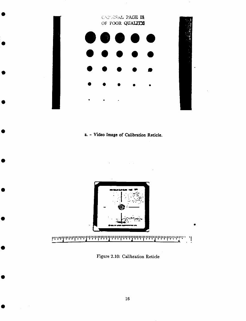
The calibration method uses a calibration reticle (i.e., opaque disks in the form of thin metal films deposited on glass substrate) [12]. The configuration and particle size variation of the specific

13

r----------- 1

\ i \ \ /

I / / /

/ / /

I / I

\ I / / \, I I /

I ', I I / ' / -4- I

/ /

I 0 0 v I

I N Y)

I

Figure 2.9: Two-Dimensional Calibration Technique

14

a

a

0

a

0

a

reticle (Model #RR-50-3.0-0.08-102-CF-114) used in calibration are shown in Fig. 2.10 and Table 2.1. The range in diameter of the reticle particles is 5.29 pm to 92.75 pm. The calibration reticle is well suited for the LI/VPS because it can easily be positioned in the plane of focus of the imaging optics, eliminating the need for depth of field correction.

The calibration procedure uses a revised version of the Particle Sizing Program (PSP) developed by Ahlers [7]. The modified PSP is setup to collect data (i.e., particle position, x and y pixel diameters, etc.) for a prescribed opaque disk from the calibration reticle. With the calibration reticle in the focal plane of the imaging optics, the calibration program is started. The calibration reticle is then positioned randomly throughout plane of focus with the program storing the data simultaneously. With the known diameter, the MCFs are found by Equation (2.4);

True diameter (pm) Measured diameter (pixels)

M C F =

The calculated MCF is then specified according to the particle’s center position. The data is then sorted into the perspective 50 vertical pixel intervals, and then each set of data (i.e., y pixel position, x MCF, and y MCF) is sorted according to y pixel position. With the correction factors specified as dependent variables of the y pixel position, the data can be set to the best fit curve. Figure 2.11 is a flow diagram of the aforementioned procedure. The above procedure was carried out for the 500X and the lOOOX lens. The use of a different particle from the calibration reticle being the only change in the procedure. Because the MCFs are determined in the procedure as average values over the total diameter of the particle, the appropriate particle had to be chosen to avoid excessive overlapping of calibration intervals. Also, to avoid the edge effect (Le., pixel elements being discrete implies pixels can be on or off depending on the position of the true particle’s edge), the largest available particle should be chosen.

Preliminary work showed that approximate MCF for the 500X lens was 2.1 pm/pixel, and conversely, 0.98 pm/pixel for the lOOOX lens. As implied above for the 50 pixel intervals, a calibration particle diameter of 25 pixels would minimize interval overlap and edge effects. Therefore, for 500X lens, the #16 particle (Le., 52.5 pm) was used, and conversely, for the lOOOX lens, the #7 particle (Le., 23.90 pm) was used. The results of the above procedure and a comparison of previous system calibrations with the present calibration is presented in Section 3.1.

2.2.4 Focus Method

Ahlers [ 71 performed work using polystyrene micro-spheres restrained be tween two glass micro- scope slides positioned in the plane of focus of the imaging optics. The above tests verified the methodology and calibration of the LI/VPS. As with most complex systems, development occurs in stages, therefore Ahlers constructed a particle sizing system which performed analysis on static and semi-static particles in the focal plane of the imaging optics with good accuracy. Wiles [lo], in the next stage in the development of the LI/VPS, defined a method of focus classification (Le., particles unaffected by diffraction light scatter). As Fig. 2.12 shows, with a diffraction limited system, particle focus is dependent on the particle’s boundary gradient and it’s relative intensity as compared to background. Because of the 8-bit precision of the video processor, the particle’s intensity level with respect to background could be used as a viable criteria for focus. The particle’s boundary gradient (PBG) was used as a secondary test because it rejects large out of focus particles which appear as small particles in focus by the particle intensity level test [lo].

With the 256 grey level resolution and the processing capabilities of the video processor, the focus parameters are determined. The particle’s intensity level or measured average grey level

15

e 0 0

e

0

0 0

0

0

a

a. - Video Image of Calibration Reticle.

Figure 2.10: Calibration Reticle

e

16

0

0

0

0

0

0

0

Table 2.1: Specification Sheet for Calibration Reticle

CALIBRATION RETICLE : RR-50-3.0-0.08- 102-CF - # I 14

FINAL DATA SHEET^

DIAMETER AREA VOLUME ( i d 2 NUMBER FRACTION FRACTION

5.29 6.8 1 8.98

11.93 17.20

6 21.33 7 23.90 8 26.71 9 31.11

10 34.17

11 37.07 12 40.47 13 42.71 14 47.37 I5 50.39

16 52.50 17 56.23 18 60.70 19 67.04 20 73.48

21 80.58 22 86.99 23 92.75

2898 776 895

1171 1009

642 456 505 396 280

306 240 207 160 106

109 96 88 58 27

11 4 1

0.0 15 0.006 0.0 13 0.030 0.054

0.053 0.047 0.065 0.069 0.059

0.076 0.071 0.068 0.065 0.049

0.054 0.055 0.058 0.047 0.026

0.013 0.005 0.002

0.002 0.00 I 0.003 0.009 0.023

0.028 0.028 0.043 0.054 0.050

0.070 0.072 0.073 0.077 0.061

0.071 0.077 0.089 0.079 0.048

0.026 0.0 12 0.004

TOTAL 1044 1 1 .ooo I .ooo

0 D(10) = 17.81 pm

D(30) = 27.69 pm

D(20) = 23.04 pm

D(31) - 34.48 pm

D(21) = 29.73 pm

D(32) = 40.01 pm

0 ~

Reproduced from specification sheet supplied by the manufacturer.

' Diameters traceable to NBS Part. #52577, accurate to f 2 pm (f 3% for D > 70 pm)

17

0

P= a I w

P; P, !H

o v j

i

-+

Figure 2.11: Flow Diagram for Calibration Procedure

18

In-focus 92.75 pm Particle.

a

a

a Out of Focus 92.75 prn Particle.

Figure 2.12: LI/VPS Focus

19

a

e

a

a

a

a

a

(MAGL [lo]) is calculated by thresholding the image at the optimum value (i.e., 90 T as specified by Ahlers), summing the pixel grey levels (GL) corresponding to specific particles as specified by segmentation, and dividing by the total number of pixels per particle (Equation 2.5).

The PBG is determined by thresholding the image twice, once at 90 T, and the second, just below background (Tb). Referring to Fig, 2.12, the double threshold specifies the particle boundary gradient by:

PBG = Dd - Db, (2-6)

where Db is the particle diameter at Tb. With the above parameters, focus was specified for a volume centered on the focal plane of the transfer lens. First, a relation, constant with respect to focal volume, was determined for the MAGL with dependence on particle diameter, and second, the PBG was specified as a constant over the range of particle diameters specified by the MAGL criteria.

In conclusion, Wiles developed a focus criteria for the LI/VPS. In his follow-up tests, the criteria defined a depth of focus which remained fairly constant when tested with the reticle and the polystyrene spheres (i.e., 52.5 pm as specified earlier). The prescribed depth of focus was approximately 400 microns. It should be noted, Wiles’ focus classification was determined and tested with the laser pulsing at 60 Hz. Thus, the focus criteria specified a depth of focus and classified particles based on grey level intensity from these operating conditions.

2.2.5 Modifications

The final goal of this research was the implementation of a particle sizing system capable of performing analysis on two- phase flow (e.g., aerosol sprays). The LI/VPS has been developed in stages; (1) Ahlers’ initial work, hardware and software setup, (2) Wiles’ work on system focus classification, and (3) the the current adaptation of the system to process truly dynamic particles in a real spray. To clarify the above statement, previous work by Ahlers and Wiles was performed with the LI/VPS operating in the continuous pulse mode (CPM), as opposed to the current work in the single pulse mode (SPM) (;.e., CPM suggests the imaging laser is pulsing at 60 Hz. in sync with the camera, and SPM implies the imaging laser is off until the video processor requires a new frame to process at which time the imaging laser is pulsed). The following discussion covers the reasoning and implementation of the SPM, and the adaptation of the previous work to function in the SPM.

All previous work on the LI/VPS was done in the CPM, therefore the system had to be converted to the SPM. The reasoning for the conversion is shown in Fig. 2.13. The two graphs were taken with the system in the CPM; the only difference being the bottom particle is dynamic whereas the top particle is stationary. As shown, there is a significant reduction in intensity for the dynamic particle as opposed to the stationary particle. The above behavior is due to the camera tube’s ability to refresh between successive frames. In the CPM, the dynamic particle being frozen by the 10 ns laser pulse is present in the field of view for less than 16.67 ms (i.e., the time necessary to complete one field), but the static particle in the CPM shows greater intensity because of the cumulative effect of the particle blanking out the same area on the camera tube. The behavior being time-dependent implies the camera tube reaches a constant intensity after a sufficient amount of time. Because the software was developed for the system operating in the CPM, and all previous

20

a

0

0

a

a

0

0

a

a

a. - Static 92.75 pm Particle in the CPM.

b. - Dynamic 92.75 pm Particle in the CPM

Figure 2.13: Static vs. Dynamic Particle Representation in CPM

21

0

work was performed on static particles (i.e., particles which have motion but appear static to the system), the system had to be adapted to size dynamic particles. Revision to the system could be achieved by either changing the system software, or changing the system hardware. Figure 2.14 shows the, MAGL vs. particle size, focus classification curves. As is shown, the ‘dynamic’ curve is less distinct than the ‘static’ curve. Because of the added ambiguities in the ‘dynamic’ curve, a method had to be determined to simulate the behavior of the stationary particles for the dynamic particles.

Because of the amount of work put into the development of the system software and the success of the focus criteria, a hardware modification was selected to accomplish the intensity contrast in dynamic particles. The SPM was found to exhibit the same characteristic intensity in the dynamic particles as found in static particles, in fact, the contrast between particle and background was greater. The SPM was accomplished by; (1) sending a trigger signal from the control computer to the LSC, (2) the LSC triggers the Nz laser, (3) the laser pulses, and (4) the image processor grabs the frame just illuminated. The above procedure was accomplished by the development of a triggering circuit (APPENDIX B). The above procedure is then followed by normal program execution. The flow diagram in Fig. 2.15 shows the SPM integrated into the PSP with software modification.

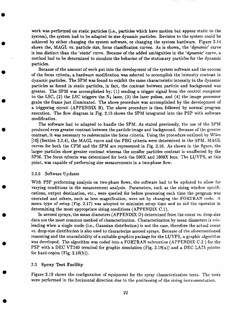
The software had to adapted to handle the SPM. As stated previously, the use of the SPM produced even greater contrast between the particle image and background. Because of the greater contrast, it was necessary to redetermine the focus criteria. Using the procedure outlined by Wiles [lo] (Section 2.2.4), the MAGL curve and the PBG criteria were determined in the SPM. MAGL curves for both the CPM and the SPM are represented in Fig. 2.16. As shown in the figure, the larger particles show greater contrast whereas the smaller particles contrast is unaffected by the SPM. The focus criteria was determined for both the 500X and lOOOX lens. The LI/VPS, at this point, was capable of performing size measurements in a two-phase flow.

0

0

0

a

2.2.6 Software Updates

With PSP performing analysis on two-phase flows, the software had to be updated to allow for varying conditions in the measurement analysis. Parameters, such as the sizing window specifications, output destination, etc., were queried for before processing each time the program was executed and others, such as lens magnification, were set by changing the FORTRAN code. A menu type of setup (Fig. 2.17) was adopted to minimize setup time and to aid the operator in determining the most appropriate sizing conditions (APPENDIX C.l).

In aerosol sprays, the mean diameters (APPENDIX D) determined from the count vs. drop-size data are the most common method of characterization. Characterization by mean diameters is mis- leading when a single mode (i.e., Gaussian distribution) is not the case, therefore the actual count vs. drop-size distribution is also used to characterize aerosol sprays. Because of the aforementioned reasoning and the unavailability of a suitable graphics package for the LI/VPS, a graphic algorithm was developed. The algorithm was coded into a FORTRAN subroutine (APPENDIX C.2 ) for the PSP with a DEC VT240 terminal for graphic simulation (Fig. 2.18(a)) and a DEC LA75 printer for hard-copies (Fig. 2.18(b)).

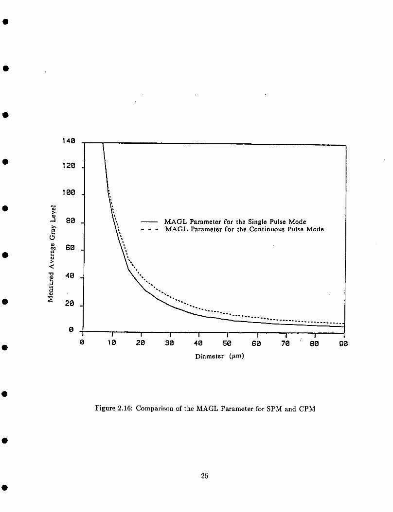
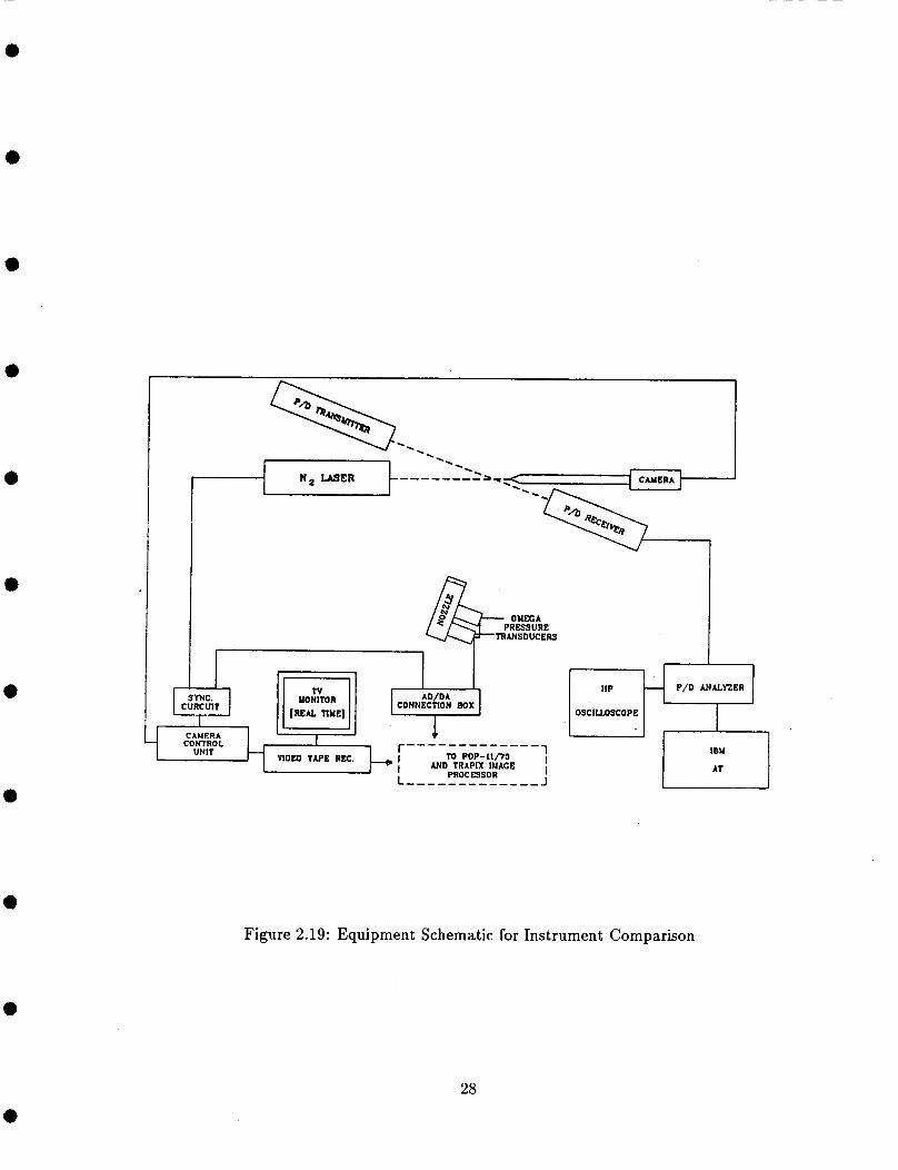
2.3 Spray Test Facility

Figure 2.19 shows the configuration of equipment for the spray characterization tests. The tests were performed in the horizontal direction due to the positioning of the sizing instrumentation.

22

a

0

140

120

100 CI a2 > 0 cl A 80 3 a2 00

0 > E 6 0

3 40 1 5

20

8

\ ' 8

I I I I I I I I 8 10 20 30 40 50 60 70 80 90

Diameter (pm)

Figure 2.14: Comparison of the MAGL Parameter for Dynamic and Stationary Particles in CPM

e

23

0

a

a

a

e

I USER INTERFACE 1 (SETUP MENU)

1 ,-q PRE-PROCESSING

I c

POST- PROCESSING

I STATISTICAL REDUCTION

w

'R- 1 Y

L r

f I RESULTS OUTPUT 1 COUNT vs. DIAMETER I DISTRIBUTION

i

(-)

SET PROCESSING PARAMETERS AND OUTPUT OPTIONS

SEND LASER TRIGGER F R W E QUALIFICATION THRESHOLD IMAGE

S ECbUZNTATIO N TECHNIQUE APPLIED

DEPEAMINE IMAGE FOCUS AND DATA ACCEPTANCE

BOUNDARY IMAGE ANALYSIS

PROCESS DATA FOR RESULTS

INTERRUP OPTIONS 'S' FOR S F N P MENU "R' FOR PROCESSING RESTART '1' FOR EXIT INTERRUP

STORE DATA ON DISK DISPLAY GENERAL DATA

GRAPHICAL PRESENTATION O F PARTICLE SIZE DATA

AS SPECIFIED ABOVE

Figure 2.15: Flow Diagram for the Particle Sizing Program in SPM

a

24

e

140

120

100

80

60

4 0

20

e

MAGL Parameter for the Single Pulse Mode MAGL Parameter for the Continuous Pulse Mode

I I I I I I I I 50 60 70 80 80 20 30 4 0 0 10

Diameter (pm)

Figure 2.16: Comparison of the MAGL Parameter for SPM and CPM

25

a

BRIGI'NU PAGE IS OF POOR QUALITX

SETUP PARTICLE SIZING PROGRAM (ver. 4 )

-_ - - -_ -_- -_ - -___-_- - - - - - - - - - - - - - PROCESSfNO OPTIONS __________- -_- - -_ - - - - - - - - e ( A ) DYNAMC Type of Processing (STATIC/DYNAMIC) ( 8 ) YES Focus Criteria (YES/NO ) (C) AUTO Type of Frame Advance (AUTO/SINCLE) (D) PARTCL Processing Limit (TIME/FRAME/PARTICLE) (E) ( 1000) Limiting Value (aeconds/framea/partlclaa) ( F ) REJECT Boundary Particles (PROCESS/REJECT)

(G) YES General Results (to PRINTER) (YES/NO)

(HI NO Average Particle sieo data -- (L) PILE: (TEHPOl).OUT

(J) YES Per Frame data ------------- > (M) FILE: (TEMPOl).DAT

( N ) Group Start s( 5 ) (0) Group Width = ( 5.0) (PI tl of Groups = ( 6 8 ) (0) X Windov Start = ( 50) (R) X Wlndov Width = ( 4 5 0 ) (S) Y Windov Start 8 ( 50) (T) Y Window Width * ( 4 5 0 )

( W ) Markers = NO (YES/NO) ( U ) Threshold = ( 90) (V) Lens = HIGH

( X ) to exlt SETUP menu or ( 2 ) to begln Partical SlEing Program .... Enter Letter to change specific Parameter 7 7

--------------r-------------------- OUTPUT OPTIONS . . . . . . . . . . . . . . . . . . . . . . . . . . WRITE TO PILE (YES/NO) (I[) FILE H E A D E R (4 lines)

( I ) NO Group Breakdovn data --------- / - - - - - -__-_--_-______-- - - - - - - - - - - - - GENERAL OPTIONS _----_---_---_--___-------

- - -_ - - - - - - - -_ -__- - - -_5__________________- - - - - - - - - - - - - - - - - - - - - - - - - - - - - - - - - - - - -

a

a

Figure 2.17: PSP Setup Page

26

a ORIGINAL PAGE Is OE POOR QUALITX

e

e

a

e

I d d m I O * # S , , ,

a. - DEC VT240 Terminal for Screen Emulation.

e

OUECA PRESSURE

TRANSDUCERS

I I I

P/D ANALYZER

OSCIUSCOPE

I IBY

Figure 2.19: Equipment Schematic for Instrument Comparison

28

*

0

a

a

e

a

a

The experimental apparatus was situated on a Newport Research optical table equipped for isolation. The building ventilation system was used to draw off the aerosol spray after analysis. The spray characterization tests were performed on an air-assist nozzle.

2.3.1 MOD-1 Nozzle

Figure 2.20 shows the MOD-1 nozzle as supplied by NASA Lewis Space Research Center. The nozzle is of the atomizer type and a prototype of the nozzle proposed to be used in the NASA Altitude Wind Tunnel to simulate various cloud structures in icing studies. Variation of the drop- size in the aerosol spray produced by the nozzle is obtained by varying the input air and water pressures. The water is introduced into a 1.81 inch- by-0.368 inch diameter mixing chamber through a 0.0155 inch orifice. The air is introduced into the outer wall of the mixing chamber through twelve 0.125 inch holes. After mixing, the aerosol is expelled from the mixing chamber through a 0.125 inch orifice.

2.3.2 Air and Water Supply System (AWSS)

As shown in Fig. 2.21, the AWSS was constructed to supply air and water to the MOD-1 nozzle with the exception of the LI/VPS optics purge. The air for the AWSS is supplied by twin 100 hp Ingersoll-Rand turbine compressors with a delivery rate of 800 SCFM at 120 psig. Because of the high water pressure necessary for the MOD-1 nozzle, a Brunswick 20.5 liter pressure vessel was filled with water and pressurized by the supply air or for higher pressures by a regulated high pressure Nz bottle. After pressurization, the water was filtered by a ADKIN spool filter. The nozzle air and water supply was regulated by a WATTS Model 2235 pressure regulator and a Cole- Palmer Model PR004-FM044-40G flowmeter, respectively. Connection lines in the supply system were YELLOW JACKET Model WPP0031A charging hose (500 max. psi.). The LI/VPS optics purge used a regulated high pressure N2 bottle for a constant positive flow from the lens cover to avoid con taminat ion.

2.3.3 Water Flowmeter Calibration

The Cole-Palmer flowmeter was factory calibrated. The calibration was verified by collecting and weighing the water passing through the flowmeter. The water was weighed on a HOWE model #3074131 balance scale. Twelve flow rates were measured with three samples collected at each flow rate. The experimental data and factory calibration data are presented in Table E13.1 with graphical representation shown in Fig. E.13.1 (APPENDIX E).

2.4 Digital Pressure Acquisition

The digital pressure system (DPS) was developed to monitor the essential input conditions of the MOD-1 nozzle. The DPS consists of two OMEGA Model PX304-15OAV pressure transducers, a DEC AXV11- C analog to digital (A/D) converter board, the PDP- 11/73 microcomputer hosting the above A/D board, and a PDP RT-11 software package written to access the A/D board and store or display the resulting pressures.

29

0REINA.L PAGE IS .OE POOR QUALITY

a. - MOD-1 Schematic.

s r i i w s s S T E E L

001 06 08 01 09 E 3P

b. - MOD-I Components.

Figure 2.20: MOD-1 Nozzle

30

MOD-1 Nozzle

._._.-.-.- ._._.-.-.- ............................... _._._._._._.-.-.-.- - . - Exhaust - ventilation t _._._._.-._._._._._._

/ I * 1

\ Iil : I lil

:r- Pressure Transducers

‘ I Air i4 0.;

Regulator i .....q- ........................... (: : .......................... .......................... :)

LIS optics purge

i Water pressurization Air system supply

..............................

Water fl Flowmeter

: a ....... N, supply , fi ..... . . . . . . .

------ . ------ e-----

--e--

111 - -- - - - - ~ - ...........................

1 ........................................................ q ........

T

:T :..4 ........ i

@-I overflow

! A 1

I Yater I ’ . . J Water sup ply

............................................................................ - Iilter

.....

Figure 2.21: Air and Water Supply Schematic

31

2.4.1 Pressure Transducers

The OMEGA pressure transducers (Fig. 2.22) are bridge type strain gage transducers. The bridge excitation voltage was 10 VDC supplied by a Hewlett-Packard (Model Harrison 6200B) d.c. power supply with a bridge output of 0 to 100 mVDC. The transducers are specified to have an operating range of 0 to 150 psia with f 0.75 psi accuracy.

a

a

0

e

2.4.2 A/D converter board

The DEC AXV11-C analog-to-digital converter board was installed in the back-plane of the PDP- 11/73 microcomputer. The AXV11-C board has 12 bit digital resolution, supports up to 16 single analog input signals or 8 differential signals, A/D conversion by program, external clock, or real- time clock, and 1, 2, 4, and 8 (i.e, 10, 5, 2.5, and 1.25 volts) programmable gain settings. As recommended by the manufacturer, the 8 channel differential option was chosen to maximize analog to digital conversion, due to the 100 mV range supplied by the pressure transducers.

2.4.3

The transducer voltage signal is converted to a digital value available to the LI/VPS operator. An interface box (Fig. 2.23) was constructed to utilize the full capabilities of the AXV11-C board. The interface box has 8 A/D input ports and 2 D/A output ports using BNC connectors. The interface box is linked to the AXV11-C board by RS232 cable and connectors. The pressure measurements are made available to the analyst through the PDP-11/73 microcomputer. The RT-11 software package, written in FORTRAN subroutine form (APPENDIX C.3), allows for real-time pressure monitoring with storage and averaging capabilites for the duration of the main calling program. The A/D converter is programed for a gain setting of 8 (i.e., an effective analog input range of 0 to 1.25 volts) to optimize A/D conversion of the pressure transducer output range of 0 to 100 mV.

Analog- t e Digit al Conversion

2.4.4 Digital Pressure System Calibration

The pressure transducers were calibrated for various static pressures by pressurizing the transducers and reading the A/D output after a steady equilibrium state had been attained. A laboratory grade test gage was used to measure the “standarb” pressure, The test gage, with a range of 0 to 160 psig, was calibrated using an American Steam Gage Co. deadweight pressure gage tester. With the pressure transducer’s specified input pressure range of 0 to 150 psia, the calibration data was taken within a range of 0 to 110 psig ( 14.05 to 124.05 psia). The atmospheric pressure at the time of the calibration run was measured to be 727.29 mm Hg. or 14.05 psia from a Precision Thermo & Inst Co. model #2769 barometer. The experimental data is presented in Tables F14.1 and F14.2 with graphical representation shown in Figs. F14.1 and F14.2 (APPENDIX F).

2.5 Experimental Procedure

With system performance and verification as the basis for comparison, equivalent sampling was required. As discussed earlier, the P/DPA and the LI/VPS use different methods of particle sizing (i.e., temporal vs. spatial), but each instrument uses a probe volume for data collection. Therefore, system comparison was dependent on spray density, droplet size range, and user designation of the measurement volumes (Le., the P/DPA’s crossed-beam intersection volume, specified by

32

e

ORIGINAC PAGE IS OF POOR QUALITY

e

Model # - PX 304-150A V

a

e

a

0

a

e

e

SPECIFICATIONS Excitation: 10 VDC Output: 0 to 100 mV Sensitivity: 10 mV/V 21%

Input Impedance: 1200 ohm Output Impedance: 500 ohm

PERFORMANCE Accuracy: *OS% full scale Zero Balance: k2.0940 full scale Operable Temperature Range:

-29 to 60" C

a. - OMEGA Pressure Transducer Data Sheet.

b. - OMEGA Pressure Transducers.

Figure 2.22: OMEGA Pressure Transducers

33

0

e

0

SCHEMATIC FOR AD/DA CONNECTOR BOX

BNC CONNECTORS

NOTE For further documentation refer 10 PDP-I1 Microcomputer Interface Hsrldtrook page 70.

E232 BNC Pin 1 - CH. 1 1 Pin 2 - CH. 2 2 Pin 3 - CH. 3 3 Pin 4 - CH. 4 4 Pin 5 - CH. 5 5 Pin 6 - CH. 6 6 Pin 7 - CH. 7 7 Pin 8 - CH. a a

9 Pin 12 - DA #l Pin 14 - CH. 1 Return Pin 15 - CH. 2 Return Pin 16 - CH. 3 Return Pin 17 - CH. 4 Return Pin 18 - CH. 5 Return Pin 19 - CH. 6 Return Pin 20 - CH. 7 Return Pin 21 - CH. 8 Return Pin 24 - DA #l Return

Figure 2.23: A/D Connector Box Schematic

34

a

a

0

a

a

a

the transmitter lens chosen and beam diameter, vs. the LI/VPS focus volume, specified by the imaging optics and software).

The procedure for overlapping the probe volumes is described in reference [14]. Figure 2.24 is included to show the scattered light, from drops generated by the VOAG passing through the crossed-beam intersection volume, as seen by the LI/VPS.

2.5.1 Verification Tests

The P/DPA and the LI/VPS probe volumes for the verification tests were specified as follows; the P/DPA transmitter lens with the 495 mm focal length and 25 mm beam separation formed a probe volume with an approximate 160 pm waist diameter, and for the LI/VPS, the lOOOX lens specifies a 400x400~140 pm3 volume with software selectable field of view for a 160~160x140 pm3 volume (Fig. 2.25).

With the above configuration, the P/DPA and the LI/VPS were tested using'a TSI Model 3450 Vibrating Orifice Aerosol Generator (VOAG). Operating conditions of the VOAG were varied to generate a size range of particles, 19.8 to 99.6 pm (Table 2.2).

Table 2.2: Verification Test Conditions ORIFICE DISTURBANCE WATER THEORETICAL

TEST DIAMETER FREQUENCY FEED RATE DIAMETER (#I (P-4 (HzJ ( cm3/min)

1 10 330.4 0.080 19.8 2 20 100.2 0.139 35.5 3 20 79.2 0.139 39.0 4 20 62.5 0.139 41.5 5 20 51.6 0.139 44.2 6 20 41.6 0.139 47.5 7 50 30.1 0.590 85.6 8 50 25.5 0.590 90.4 9 50 19.0 0.590 99.6

Each particle size generated either in single stream form or using the dispersion cup (Fig. 2.26)to generated a spray was measured using the P/DPA and the LI/VIPS system. The TSI droplet diameter (Dd) was calculated using the TSI theoretical equation (2.7); a

where q is the liquid flow rate and f is the disturbance frequency. Results of the tests are presented 0 in Section 3.2.

35

a

ORIGINAL PAGE IS W POOR QU-

a

a

Figure 2.24: P/DPA Doppler Fringes as Seen by the LI/VPS Imaging Camera

a

a

Figure 2.25: P/DPA and LI/VPS Over-lapping Probe Volumes

36

a

e

a

ORIGINAL PAGE IS OF POOR QUALITY

/Disoersed Droolet

Dispersion Orifice oirwrsion cover

.. r O r i l k e Disc

a. - VOAG Dispersion Cup.

b. - TSI Vibrating Orifice Aerosol Generator.

Figure 2.25: Verification Test Apparatus

37

e

e

a

e

2.5.2 Spray Comparison

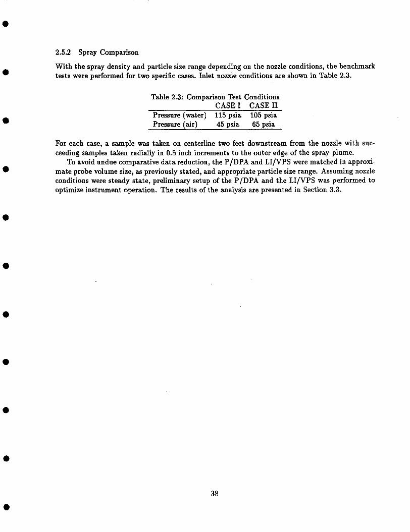
With the spray density and particle size range depending on the nozzle conditions, the benchmark tests were performed for two specific cases. Inlet nozzle conditions are shown in Table 2.3.

Table 2.3: Comparison Test Conditions CASE1 CASE11

Pressure (water) 115 psia 105 psia Pressure (air) 45 psia 65 psia

For each case, a sample was taken on centerline two feet downstream from the nozzle with succeeding samples taken radially in 0.5 inch increments to the outer edge of the spray plume.

To avoid undue comparative data reduction, the P/DPA and LI/VPS were matched in approximate probe volume size, as previously stated, and appropriate particle size range. Assuming nozzle conditions were steady state, preliminary setup of the P/DPA and the LI/VPS was performed to optimize instrument operation. The results of the analysis are presented in Section 3.3.

e

e

38

a

f 2.21 + y * 0.803E - 04 for 50 5 x < 100 2.20 i- y * 0.290E - 04 for 100 5 x < 150 2.16 + y * 0.679E - 04 for 150 5 x < 200 2.16 + y * 0.442E - 07 for 200 5 x < 250 2.16 - y * 0.947E - 04 for 250 5 x < 300 2.11 - y * 0.306E - 07 for 300 5 x < 350 2.10 - y * 0.124E - 03 for 350 5 x < 400 2.07 - y * 0.135E - 03 for 400 5 x < 450,

a

Section 3

a

a

0

a

0

a

a

PRESENTATION AND DISCUSSION OF RESULTS

This section will present the results of the LI/VPS calibration tests including a comparison with previous calibration tests, the verification tests with the VOAG, and the comparison tests using the MOD-1 nozzle. The major concern of these results is the accuracy of the sizing measurements with secondary interest in the comparability of the LI/VPS and the P/DPA.

3.1 LI/VPS Calibration Results

As was stated previously, the LI/VPS had to be recalibrated due to the replacement of the vidicon camera tube. With the new vidicon tube, the MCF became approximately 2.1 pm/pixel (i.e., for the 500X lens), as opposed to the previous factor of 1.8 pm/pixel [7,10], for the old camera tube. The new vidicon tube, therefore, reduced the LI/VPS measurement resolution. The above is mentioned to explain the increased error in determining the smaller particle sizes for the 500X lens, as well as the reasoning for the calibration of the lOOOX lens. The following calibration results specify the MCFs for the 500X and the lOOOX lens. Results of previous calibration tests using the calibration reticle have been compared to the new calibrations.

Using the procedure described in Section 2.2.3, the Equations (3.1) thru (3.4) represent the MCFs as functions of x and y location for the two lens;

the xMCF for the 500X lens;

M C F ( y ) =

39 a

the yMCF for the 500X lens;

0

MCF(y)=

the xMCF for the lOOOX lens;

0

MCF(y) =

e

' 2.10 - y * 0.183E - 03 for 50 5 x < 100 2.11 - y * 0.240E - 03 for 100 5 x < 150 2.12 - y * 0.314E - 03 for 150 5 x < 200 2.13 - y * 0.313E - 03 for 200 5 x < 250 2.15 - y * 0.397E - 03 for 250 5 x < 300 2.18 - y * 0.484E - 03 for 300 5 x < 350 2.19 - y * 0.505E - 03 for 350 5 x < 400 2.18 - y * 0.509E - 03 for 400 5 x < 450,

and the yMCF for the lOOOX lens;

a

e

a

' 0.977 + y * 8.09E - 05 for 50 5 x < 100 0.974 + y * 2.60E - 05 for 100 5 x < 150 0.967 - y * 8.12E - 07 for 150 5 x < 200 0.961 + y * 4.73E - 06 for 200 5 x < 250 0.961 - y * 5.46E - 05 for 250 5 x < 300 0.948 - y * 3.72E - 05 for 300 5 x < 350 0.943 - y * 6.80E - 05 for 350 5 x < 400 0.920 - y * 2.583 - 05 for 400 5 x < 450,

0 ' 0.977 - y * 9.17E - 05 for 50 5 x < 100 0.981 - y * 1.24E - 04 for 100 5 x < 150 0.981 - y * 1.19E - 04 for 150 5 x < 200 0.990 - y * 1.63E - 04 for 200 5 x < 250 1.000 - y * 1.96E - 04 for 250 5 x < 300 1.014 - y * 2.19E - 04 for 300 5 x < 350 1.027 - y * 2.636 - 04 for 350 5 x < 400 1.029 - y * 2.69E - 04 for 400 5 x < 450.

(3.3)

(3.4)

With the above equations, a software algorithm was setup in subroutine form to determine the correction factors as functions of particle location and for the magnification lens installed (APPENDIX

Figures 3.1 - 3.4 show the variation of the MCFs with respect to x and y location. The similarity in Figs. 3.1 and 3.3, as well as the similarity in Figs. 3.2 and 3.4 show the MCFs' variation is mainly due to the geometric non-linearities in the vidicon tube. The procedure developed to determine the MCFs as functions of both x and y screen location is easy to use, straight-forward, and not time consuming. The implementation of the MCFs in PSP is easily facilitated by the use of the FORTRAN subroutine format.

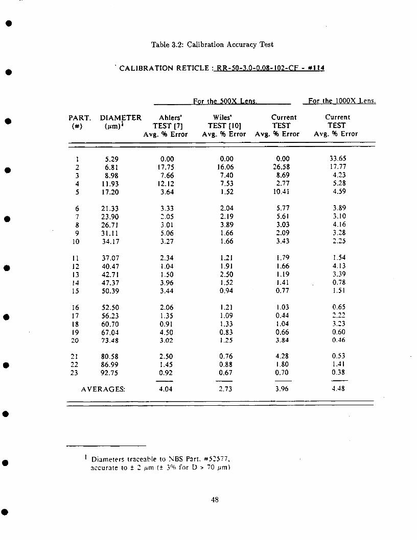
The following comparison represents LI/VPS accuracy studies by this investigator and the previous investigators [7,10]. The basis for the comparison was the utilization of the calibration reticle with the 500X lens. Table 3.1 shows the results for the 500X lens by this investigator. Table 3.2 represents the equivalent results for the lOOOX lens under similar test conditions.

C.4).

40

e

e

e

e

e

e

e

0

X Magnification Corrcction Factor for the SOOX Lens

Figure 3.1: Magnification Correction Factor Behavior

e

41 e

2.16

.d

E W

I .96

I'JO

Y Mnnnification Correction Factor for the SOOX Lens


42

0

0

0

X Magnification- Correction Factor for the IOOOX Lens


0

43

Y Magnification Correction Factor for the IOOOX Lens


e

44

N

I & 0

. & b h > w 4

0 N

-4 (3

0 . . n .. m %6 4 m h rl 0

Q

% .

2" h a 0.4

5 C 4

e !

I I l O d 0 n 0 n G d ~ ~ ~ ~ d r o ~ 1 m ~ 1 w m ~ n i n i o n n ~ ~ 1 n 0 m i n 1 w r o n n ~ n n n ~ n w i n I . . . . . . . . . . . . . . . . . . . . . . . . . l 0 0 0 0 0 0 0 0 0 0 0 0 0 0 0 0 0 0 0 0 0 0 0 l 0 I I

I 1 1 1 1 1 1 1 l I 1 1 l 1 1 1 1 I I 1 1 1 1 1 1 I I

I O N P ~ P O ~ O O N O ~ ~ ~ G ~ O O ~ Q O N ~ I . . . . . . . . . . . . . . . . . . . . . . . l O 1 P O n O N w m Q w 0 O P m m n O n 4 0 w o I ~ ~ N N N N O ~ O Q Q Q Q U I ~ O F F ~ ~

I

3- i C r l O O O O O O o O O O O O O O O O O o o o o o o 2 - 1 nnnnnnnnnnnnnnnnnnnnnn

8 1 a r l l ..

m

a v Y

.. z

a

45

Q

I I t n d 0 n ~ n a , d ~ ~ r - r - d n r ~ n d n ~ ~ o a , 0 1 0 1 0 n ~ n n ~ d n 1 1 d n 1 n n n ~ 1 1 n 1 n ~ i n I ....................... I . 1 P I 0 0 0 0 0 0 0 0 0 0 0 0 0 0 0 0 0 0 0 0 0 0 l 0 I I

.. @? m

46

e

0

a

0

e

e

0

0

Table 3.3 shows the average percent error for the above calibration accuracy tests with the previous work of Ahlers [7] and Wiles [lo]. A comparisbn of the average % error for the three accuracy tests performed on the 500X lens shows a decrease in the % error from the one- dimensional MCF test (Le., 4.04% error) to the twedimensional MCF tests (i.e., for Wiles - 2.73% error and for this work - 3.96% error). The % error values for the test performed on the lOOOX lens show an increase in LI/VPS accuracy for all the particles measured by the 500X lens tests. The inclusion of the 5.29 pm particle in the analysis shows an increased sizing range, as opposed to previous tests.

The following results represent the initial method used to compare the P/DPA and the LI/VPS. As specified earlier, the probe volumes of the two instruments were overlapped, and due to the steady state operation of the VOAG, samples by both instruments were assumed to be nearly identical. Two separate cases were performed to verify instrument operation and accuracy. The first case was performed with the VOAG producing a steady single stream of drops which passed through the concurrent probe volumes, and secondly, the dispersion cup (Fig. 2.26) was utilized to produce a spray of monodisperse droplets which randomly pass through the concurrent probe volumes. Nine separate tests were performed for each case with the instrument results represented in Figs. 3.5 thru 3.13 for the case without the dispersion cup, and Figs. 3.14 thru 3.22 for the case with the dispersion cup. Figures 3.23 and 3.24 show the TSI theoretical diameter, and the arithmetic mean diameters from the LI/VPS and the P/DPA distributions as functions of test number. Data in Table 3.4 has been plotted in Fig. 3.23 and 3.24 with the standard deviation (SD) also shown. The arithmetic mean diameters of the LI/VPS and the P/DPA agree, on the most part, with each other and the theoretical expected diameter within f 2.6 pm. The SD of the samples is shown to illustrate the monodisperse behavior of the VOAG and the ability of the LI/VPS and the P/DPA to measure the monodisperse aerosol spray. The highest SD (i.e., 1.109 pm) determined for the LI/VPS is shown in CASE I1 - Test 5, and for the P/DPA, the highest SD (Le., 2.073 pm) is shown in CASE I - Test 1.

Referring to Table 3.4, the first test in both cases show the maximum SD for P/DPA. The arithmetic mean diameters, 20.5 pm for CASE I and 21.5 pm for CASE 11, are within 2.0 pm of the expected diameter, 19.8 pm. The SD of the samples may be higher than the rest, due to the high density of drops passing through the P/DPA probe volume. This phenomena was especially noticeable in CASE I1 test runs where the dispersion cup was used. As was expected, the SD for most of the tests increased from CASE I to CASE 11. The above behavior was expected, due to the increase in number of drops passing through the edges of the probe volumes.

3.2 Results For the MOD-1 Nozzle Comparison

The following results represent a comparison of the LI/VPS and the P/DPA in side-by-side benchmark tests performed on a NASA MOD-1 atomizing nozzle. As previously stated, two cases (Le., variation in the operating conditions of the nozzle) were studied. For each case, eight data runs (Le., a data run was performed on the centerline, two feet down-stream from the nozzle with succeeding data runs performed at one-half inch increments radially outward to the edge of the dispersion) were performed by the LI/VPS and the P/DPA using a procedure similar to the VOAG analysis. Figures 3.25 - 3.32 and Figs. 3.33 - 3.40 are the results from the P/DPA and the LI/VPS for CASE I (Le., nozzle conditions: Air pressure = 65 psia and Water pressure = 105 psia.) and CASE I1 (Le., nozzle conditions: Air pressure = 45 psia and Water pressure = 115 psia), respectively.

47

a

a

Table 3.2: Calibration Accuracy Test

' CALIBRATION RETICLE : RR-50-3.0-0.08 -102-CF - #114

For the 500 X Lens. For the IOOOX Lens.

PART. DIAMETER Ahlers' Wiles' Current Current (#) ( c r d TEST [7] TEST [ 101 TEST TEST

Avg. % Error Avg. % Error Avg. % Error Avg. % Error

0

0.00 17.75 7.66

12.12 3.64

0.00 16.06 7.40 7.53 I .52

0.00 26.58 8.69 2.77

10.41

33.65 17.77 4.23 5.28 4.59

1 5.29 2 6.8 1 3 8.98 4 11.93 5 17.20

a

6 2 1.33 7 23.90 8 26.71 9 31.1 1

10 34.17

3.33 2.05 3.01 5.06 3.27

2.04 2.19 3.89 1.66 I .66

5.77 5.6 1 3.03 2.09 3.43

3.89 3.10 4.16 3.28 L . d 3 3 -

0

1 1 37.07 12 40.47 13 42.7 1 14 47.37 15 50.39

2.34 1.04 1 .so 3.96 3.44

1.21 1.91 2.50 1.52 0.94

I .79 1.66 1.19 1.41 0.77

1.54 4.13 3.39 0.78 1.51

a

16 52.50 17 56.23 18 60.70 19 67.01 20 73.48

2.06 1.35 0.9 1 4.50 3.02

1.21 1.09 1.33 0.83 I .25

I .03 0.34 1.04 0.66 3.84

0.65 2.22 3.23 0.60 0.36

21 80.58 22 86.99 23 92.75

2.50 I .45 0.92

0.76 0.88 0.67

4.28 I .80 0.70

0.53 1.31 0.38

4.48 4.04 2.73 3.96 AVERAGES:

Diameters traceable to NBS Part. tt52577, accurate to ?: 2 /in1 ( + 3% for D > 70 pm) 0

48

0

C

0

0 ' U

0

I

I

e

8 0 0 - I I

Spatial Distribution . . . . . . . . Distribution M e Dia. = 19.5

YI Surface Mean Dia. (D20) = 19.1 t- Volume (Hass) kan Dia. (D30) = 19.1 2 Sauter h a n Dia. (043) = 19.1

600 - r bithetic Hean Dia. (DlO) = 19.1 -

J

u 400 -. Total Count = 1009 -

2 0 0 -

0 . I 5.0 22.5 40.0 57.5 75.0

a

201 .6 Nost Probable Dia= 18,6

llrithnetic Mean (D10): 20,s llrea Mean (D20): 21

Uolune Mean (D30k 21,6 Sauter Mean (D32k 2 3 , l

Corrected Count : 10049 I File: VERI 01,DAT Iltny: 12634 Total Count: 19882 Date: 12-13-1986 The: 15:57:89 . Run Time: 266,290 seconds

-~ ~~~

1475 Velocity Mean = 15,8 MS velocity = ,61

C

n t Phs= 0 Sat= 5 O w = 213 Dia:

Und= 129 Ouf=

0 U

lbLl 213 4.3 12 .1 20,0 Max= 80 Uel= 0 Ueloci ty (meters/second) Total Bad = 442 BOUMSDTU

DIfWTER (aicrons)

Theoretical Diameter = 19.8 pm Diameter of Orifice = 10 p m

Liquid Feedrate = 0.08 cm3/min. Vibration Frequency = 330.4 kHz

Figure 3.5: VOAG Verification w/o Dispersion Cup

e

49

e

601- I I

Spatial Distribution . . . . . . . . Distribution Node Dia. = 36.1

Surface Hean Dia. (D20) = 36.0 Volume (Hass) k a n Dia. (D30) = 36.0

Swter k a n Dia. (D43) = 36.1

453 .’ Arithsrctic Hean Dia. (Diol = 35.9 - w k 2 3

0 302 - , Total Count = io04 -

151 - 5

0 . -- 25.0 42.5 60.0 77.5 95.0

e

a

c l 01

I I I I 1 I I “Ll

5

280 3 6 , 0 70 Diane ter (n i croMe t ers 1

4743 Most Probable Dia= 35,5

h i thmetic Mean (Dial= 35,8 hrea Mean (D29)= 35,9

Uolune Hean (D30k 36 Sauter Mean (D32k 36,3

Corrected Count : 18112 File: UERI 02,DAT Atw: 12172 Total Count: 14418 ((( 1 Date: 12-13-1986 Tine: 12:24:57 Rim T h e : 121,464 seconds

3166 Velocity nean = 6,81 RHS uelocity = .23

Phs= 0 Sat= Ovr= 47 Dia: 281 Kl Und= 445 Ovf=

Ueloci ty (neters/second) Total Bad = 1602 BOUMSDTU 0,6 4.1 7 ,7 Max= 819 Vel= 7

819

Theoretical Diameter = 35.5 pm Diameter of Orifice = 20 pm



50

Host Probable Dia: 39m2 Rri tlinetic Hean (Dl8): 39m6

Area Hean (D28): 39.6 Uolune Hean (D30): 39.6 Sauter Hean (D32): 39.6

I I Y I I I 2.6 46.3 98

Diameter (nicroneters) Corrected Count: 10304 File: VERI 83,DllT Atnp: 10338 Total Count: 18881 ((( Date: 12-15-1986 Tine: 11:23:21 Run fine: 23,985 seconds

C I I I I !, I 2172 Velocity Hean : 7m02 0 INS velocity = ,18 U n t s

0m6 41 1 7m7 Ueloci t y (ne terdsecond)

d Phs= 0 sat= e 22 Our= 7 Dia= Und: 15 Our= Max= 22 Uel:

Total Bad : 44 -

640

160

0 3c

I I

Spatial Distribution . . . I I Distribution node Dia. = 40.3 kithnetic kn Dir. (Dl01 = 39.8

surface Mean Dia. (D20) = 39.8 Volume (Mass) k a n Dia. (D30) = 39.8 it Satter.kan Dir. (D43) = 39.8

0 47:s 65:O 82:5



0


51

a

0

Most Probable Dia= 41.7 hitluretic Mean (DlUk 41.8

Lrea Mean (028): 41.8 Uolune Hean (D38k 41.8 Sauter Hean (D32k 41,9

2891 Velocity nean : 7,83 MS velocity : ,19

PIS e sat: Ow= 71 Dia:

0

a

a

0

328..

Spatial D

Distrib 246 - 4-i th

w su c Volune (

S

0 i64 *.

2 3

u

82 - '

0 - 30.0 47.5 65

DIMER

stribution . . .. . .. . ition node Dir. * 42.4 K t i c Hen Dia. ( D l O ) = 42.7 ,face Mean Dir. (D20) - 42.7 lass) Hean Dia. (D30) = 42.8 iuter tlean Dir. (D43) = 42.8

Total Count = 1001

0 82.5 100.0

(aicrons)




52

a

C 0 U n ’ t . 5

7991 Host Probable Dia= 43,5

Arithmetic Hean (D18k 43,3 Brea Hean (D28k 43,3

Uolume Hean (D30k 43,3 Sauter Hean (D32k 43.3

512

384 w t- 2 3

0 O 256

128

0 3!

C 0 U , n t . 5

1 1

Spatial Distribution . . . . . . . . Distribution ckde Dia. = 45.5 bithetic Hean Dia. (Diol = 45.2 -

Surface kan Dia. (D20) = 45.2 Voluae (Mass) kan Dia. (D30) = 45.2

Sauter k k a n Dia. (D43) = 45.2

-

7 Total Count = 1000 -

6958 Velocity Mean = 7 . 2 RM velocity : ,ll

Phs= 0 Sat: hr= 8 Dia=

D 52 I 70:0 8715 10:

DIMTER (microns) 0

Theoretical Diameter ’= 44.2 pm Diameter of Orifice = 20 pm

Liquid Feedrate = 0.139 cm3/min. Vibration F’requency = 51.6 kHz


53

e

C

n t ,

0 ’ U

S

e

II

5 4 0 -

405 - Y I. 2 3

u O 270 -

135 -

0 . 40.0

3865 Host Probable Dia: 49.2

Ari tlrnetic Mean (DlOk 49.2 Area Mean (D20)= 49.2

Volune Hean (D38k 49.2 Sauter Mean (D32)= 49.2

I

Corrected Count : 18367 File: VERI 06,DIT fttnp: 10485 Total Count: 18813 ((( Date: 12-12-1986 Tine: 84:06:15 R u n Tine: 26.249 seconds

2331 Velocity Hean = 9,25 RMS velocity = .26

PIG 0 Sat=

Und= 2.3 8 . 4 14.5 Max: 0 Vel= 0

Ueloci tu (neterdsecond) Total Bad = 472 BOUHSDTU

472

I Spatial Distribution . . . . .:. . .

I

I

Distribution Hode Dia. = 49.7 Arithnetic Hean Dia. (Diol = 48.8

Surface Hean Dia. (D20) = 48.8 Volune (Hass) Hean Dia. (D30) = 48.9

Swter Mean Dia. (D43) = 48.9

Total Count = 1001

DIMTER (microns)




54

e

e

0

a

a

e

a

a

0

Diane ter (ni crone t ers)

4744 Most Probable Dia: 86

Qrithnetic Mean (Dl0k 85 Qrea Mean (D28): 85

UoluHe Hean (D3N= 85 fauter Mean (D32)= 85

Corrected Count: 10724 File: UERI @?,DIT Atnp: 10863 Total count: ~ ~ 2 4 ((( Date: 12-12-1986 Time: 83:14:32 Run Tine: 24,2@4 seconds

3547 Uelocity Mean : 5 , 2 M velocity : ,21

n t Phs= 0 Sat= 5 Our: 0 Dia:

Und= 15 Our= 1.2 484 7 ,7 Max- 24 Uek EE!3 Ueloci t y (ne ters/second) Total Bad = 39 BMMSDTU

24 IF1

Di! A r i h t i c lkan Dia. (Diol = &I6 1

Surfacp Hean Dia. (D20) = 85.7 294 m

c z

I I

Spatial Distribution . . . . . . . . . ~tribution Hode Dia. = 86.6

1 392 -I

3 I I Volune (Haass) Mean Dia. (D30) = 85.7 Sauter kan Dia. 043) = 85.7 I

-, Total Count = I000 --!

105f0 12215 140:O

DIAKTER (aicrons)



Figure 3.11: VOAG Verification w/o Dispersion Cup e

55

e

0

C I I 0

n t 5

U

e

4661 Uelocity Mean = RHS velocity :

Phs= 0 Sat: Our= 0 Dia= Und= 32 Ovf=

0 ce

436 -.

327 * m I- 2 3

0 218 -

109 *

0 - 80.0

i i S

5.1 92.6 188 Di a~ ter ( H i crone t ers )

I I

Spatial Distribution . .. .. . .. Distribution Hode Dia. = 91.8 Arithnetic k a n Dia. (DlO) = 91.2 -

Surface tlean Dia. (D20) = 91.2 Volum (Nass) Hean Dia. (D30) = 91.2

Saute k a n Dia. (D43) = 91.2

Total Count = I000 -

I I 97.5 115.0 132.5 150.0

6460 Uost Probabl

Arithmetic Hean b e a Mean

Volume Mean Sau t er Hean

Corrected Count :

e Dia= 91,2 CDl8>= 98,3 (D28): 98,3 (D30)= 90,4 (D32k 90,5

11799 ~~

Pile: UERI 08,DAT AtHp: 10837 Total Count: 18884 ((( Pate: 12-11-1986 Time: 01:34:12 Run Tine: 24,881 seconds

5.33 I 27

IK] 8 BOU HSDTU

32

-


Liquid Feedrate = 0.59 cm3/min. Vibration Frequency = 25.5 kHz,

Figure 3.12: VOAG Verification wio Dispersion Cup

56

a

C 0 U n t , 5

a

5108 Most Probable Dia: l W 7

A r i t k t i c Mean (D18): 99.9 hwa Mean (D20): 99,9

Uolune Mean (D30k 99,9 Sauter Mean (D32): 188

a

C 0 ' U , n t 5

8119 Uelocity Nean : 5.76 RMS uelocity : .09

2 Phs= B Sat= Ovr= 8 Dia=

348- I I

Spatial Distribution . . . . .. . . . Distribution !lode Dia. = 101.3

Y Surface kan Dia. (D20) = 100.8 Volune (Ilass) kan Dia. (D30) = 101.1

Sauter kean Dia. 043) = 101.8

261 -. hihetic han Dia. (Diol = 100.3 - I- 2 3

u 174 Total Count = 975 - -

87 -

0 - . I 90.0 107.5 125.0 142.5 160.0



. Figure 3.13: VOAG Verification w/o Dispersion Cup

57

0

e

0

Most Probable Dia= 21,2 h i t h e t i c Mean (D18k 21,5

Area Mean (D28k 21,9 Uolune Mean (D30k 22,5 Sauter Mean (D32)= 23.9

2.6 46,3 Dianeter (Micrometers) Corrected Count : 18115

Pile: UERD 81.DIT Itnp: 31193 Total Count: 18804 ((( Date: 12-15-1986 Tine: 15:58:32 Run Tine: 945,886 seconds

2896 Uelocity Mean = 16,l RMS uelocity = ,61

P~S: a Sat= r-j 11846 Our= 384 Dia= Und= 158 Ouf=

4.3 12 .1 20.8 !lax= 11846 Vel= 1121 Ueloci tu (neters/second) Total Bad : 13192 BOUMSDTU

0

0

512 - I I

Spatial Distribution ......... Distribution I(0de Dia. = 19.6

a Surface Mean Dia. (D20) = 19.3 k Volune (llass) Mean Dia. (0301 = 19.3 2 Saute Mean Dia. (013) = 19.3

384 kithnetic Mean Dia. (Diol = i9.2 -

a DIAETER (microns)



Figure 3.14: VOAG Verification w/ Dispersion Cup

58

0

r I

3683 I Host Probable Dia= 35,5 I

C

m I 0 ' U Arithnetic Hean ( D L Q ) = 36.8 n Area Hean (D20k 37

Uolune Hean ( D 3 Q k 37,4 Sauter Hean (D32k 38

t

2.8 36.0 70 S

Diane t er hicrone ters) Corrected Count: lW99 File: UERD O L D A T Atnp: 12134 Total Count: 18016 ((( Date: 12-1T-1986 Tiw: 12:26:40 Run Tine: 32.745 seconds

C 2391 Uelocity ban = 6,69 0 RMS velocity : ,33 U n t 706 Phs= 1 Sat=

Our= 44 Dia: 321 Und= 499 Ovf= e, 6 4 . 1 7,7 Max: 706 Vel= 6

S

Ueloci t y tneters/second) Total Bad = 1581 BOUMDTU *

308- I I

Spatial Distribution ......... Distribution Hock Dia. = 39.3

W Surface Mean Dia. (D20) = 38.3 t Volune (Itass) Mean Dia. (D30) = 38.3 z S a u k k a n Dia. (M3) = 38.3 3 Q 151 -- Total Count = 1001 - 0

231 -' hithnetic Mean Dia. (Diol = 38.3 -

77 --

0 - '

30.0 47.5 65.0 82.5

DIAKTER (sicrons)

Theoretical Diameter = 35.5 pm Diameter of Orifice = 20 pxn


0


59

C

n t

2.6 46,3 90 Diane t e r ( mi crone t ers 1

0 U

S

C 0 U - I

2.6 46,3 90 Diane t e r ( mi crone t ers 1

7838 Velocity Mean = 7,15 RMS velocity = ,13

3723 Host Probabl

Aritlinetic Mean Area Mean

Uolune Mean Sauter Mean

412 -

309- w k z

0 2 0 6 - 3

0

103 -

Corrected Count :

I I

Spatial Distribution ......... Distribution Mode Dia. = 39.3 Arithaetic Mean Dia. (Diol = 40.2 -

Surface Mean Dia. (D20) = 40.4 Volune (tlass) Mean Dia. (D30) = 40.6

Swter Mean Dia. (D43) = 41.1

Total Count = 1001 -

e Dia= 39,2 (D10k 38,8 (D20k 38.9 (D30k 38,9 (D32k 39

I

30.0 47.5 65.0 82.5 100.0 0

11331

II I Our= 9 Dia= Und: 59 Ouf= 2844

20,9 Max= 6902 Vel: 9

t . 5

4.3 12.1 Ueloci t y (neters/second) Total Bad = 9805 BOilMSDTU

6902

-



Figure 3.16: VOAG Verification w/ Dispersion Cup e

60

a

e

340 - I I

Spatial Distribution . . . .. .. Distribution lkde Dia. = 43.4

YI Surface Mean Dia. (D20) = 43.5 Volwe (tiass) kan Dia. (030) = 43.5

2 Sautec Mean Dia. 043) = 43.6

* 174 - Total Cocmt = 1001 -

261 - kithetic k a n Dia. (DlO) = 43.5 - c

3

0

87 -

I L 30.0 47.5 6!i. 0 82.5 100.0

I 0 -

a

a

a

e

e

cl I 1 1 I 7852 Most Probable Dia: 41,7 i-1 - - - -Arit laet ic Mean (Dill)= 41,9

Area Mean (D20k 41,9 t Volume Mean (D36k 41.9 S Sauter Mean (D32k 42 2.6 46.3 90

Diane ter (microMe ters ) Corrected Count: 10232 File: UERD 9 4 , D A T htmp: 1737 Total Count: 10006 < t i I Date: 12-13-1986 Time: 11:14:18 Run Time: 1139.577 seconds

C 1786 Velocity Mean = 4.49 0 RMS velocity = 2.96 n t Phs n Sat= 28161

U

Ow= 77 Dia: Und= 24 Ovf= 1974! TTi]

Ueloci ts (neterdsecond) Total Bad = 52124 BOUMSDTU

5

0.6 4 , l 7 . 7 )Iw= 28161 Vel= 4120



Figure 3.17: VOAG Verification w/ Dispersion Cup e

61

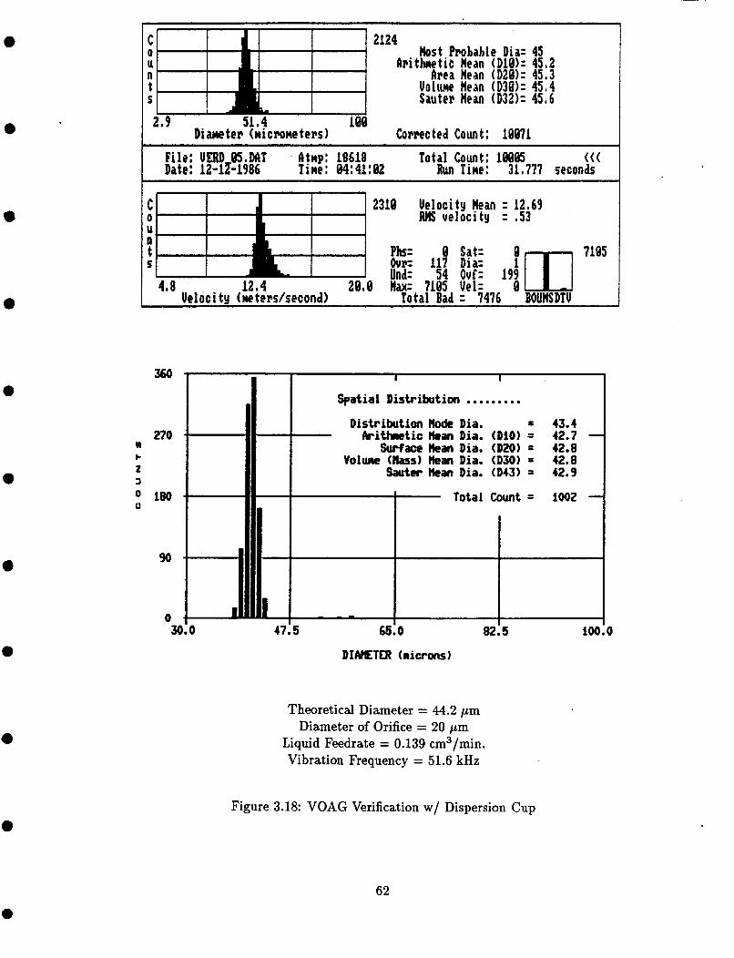
e

47: 5 65:0 8215 100.0

0

2124 Most Probable Dia= 45

Arithmetic Mean ( D l U k 45,2 llrea Mean (D2Qk 45.3

t Volume Mean (D30)= 45,4 S Sauter Mean ( D 3 2 k 45,6 2.9 51 ,4 roo !!ziIEH Di nne t er (ni crone t ers 1 Corrected Count: 10071

e

0

a

0

0

~ ~~

File: UERD 85,MT Atnp: 18618 Total Count: 10005 ((( Date: 12-12-1986 Time: 04:41:02 Run Time: 31,777 seconds

2310 Velocity Mean = 12,69 IMS velocity = ,53

l!l+&+l LE Und=

4.8 12.4 20,8 Elax= 7105 Ueloci t y (treters/second) Total Bad

360

270 Y k z 3

U 180

90

0

1: Kl Sat= Di a= Ouf = Vel= Q = 7476 BOUMSDTV

Spatial Distribution . . . . . . . . . Distribution Hock Dia. = 43.4 kithmtic Hean Dia. (Diol = 42.7 -

Surface h a n Dia. (DM) = 42.8 Voluae (flass) ban Dia. ( D 3 0 ) = 42.8

h t e r Hean Dia. (D43) = 42.9

Total Count = io02 -

-




62

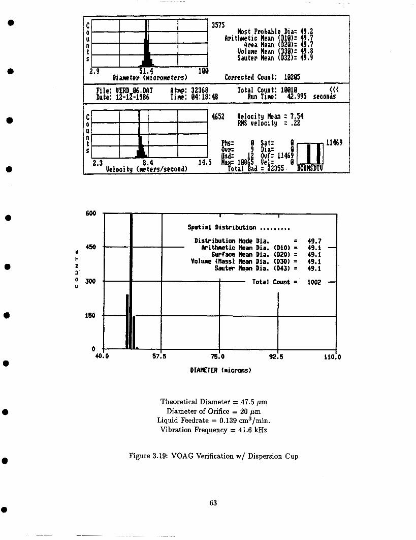
e c

Host Probable Dia= 49,2 C 3575

U Ari thnetic Mean (DlQk 49,7 n Area Hean (D20k 49.7

UoluMe Mean (D3Qk 49.8 Sauter Mean (D32k 49.9

t

0

S

51.4 100 Corrected Count : 10205

2 , 9 Diameter (nicroneters)

File: UERD B d . D A T IltMp: 32368 Total Count: 18018 ((( Date: 12-12-1986 Tine: 94:18:48 Run Tine: 42,995 seconds

4652 Uelocity Mean : 7,54 RMS uelocity : ,22

C

n t

0 U

I Phs: 0 Sat= 1 ml 11469 Our= 9 Dia= Und= 12 Owl= 11469

14.5 Max= 10865 Vel= Q S

Total Bad : 22355 BOUMSDTU 2.3 8 , 4

Velocity (neters/second) b

0

0

0

0

a

0

I I

Spatial Distribution . .. . .. ... I I Distribution Hade Dia. = 49.7 Ib-ithmetic Hean Dia. (DlO) = 49.1

Surface Mean Dia. (D20) = 49.1 Volune (Ilass) Hean Dia. (030) = 49.1

Sauter Mean Dia. (D43) = 49.1

Total Count = 1002

0

DIAXTER (nicrons 1

Theoretical Diametef = 47.5 pm Diameter of Orifice = 20 pm


e Figure 3.19: VOAG Verification w/ Dispersion Cup

63

0

d e

0

a

0

I , 1

2140 Host Probable Dia= 86,7

C U Arithnetic Nean (Dl0)= 8 6 , l n Area Nean (D20)= 86,4 t Volume Mean (D30)= 86.6 5 ' Sauter Hean (D32k 87,1

0

Diane ter (nicrometers) Corrected Count : 10720

Run Tine: 28,451 seconds File: UERD W,DM Atnp: 11468 Total Count: 10001 I Date: 12-12-1986 T h e : 03:22:42

C ( I I j I1398 Velocity yean = 9 , 7 5 . 0 RMS velocity = ,73 U n

5 t Phs= 0 Sat= Ovrz 12

Dia= I$ r u Und= 280 Out= Veloci ty ( n e t e d s e c o n d ) Total Bad = 1439 BOUHSDTU

2.3 8 . 4 14.5 Max= 148 Vel= 2

875

472 - I I

Spatial Distribution ......... Distribution flock Dia. = 87.6

M Surface Hean Dia. (D20) = 86.8 Voluae (bass) Hean Dia. (030) = 86.8

z Swter k a n Dia. (D43) = 86.8

O 236 Total Count = lo00 -

354- Arithmetic k a n Dia. (DlO) = 86.7 - k

3

u

80.0 97.5 115.0 132.5 150.0

DIAHETER (aicrons)




64

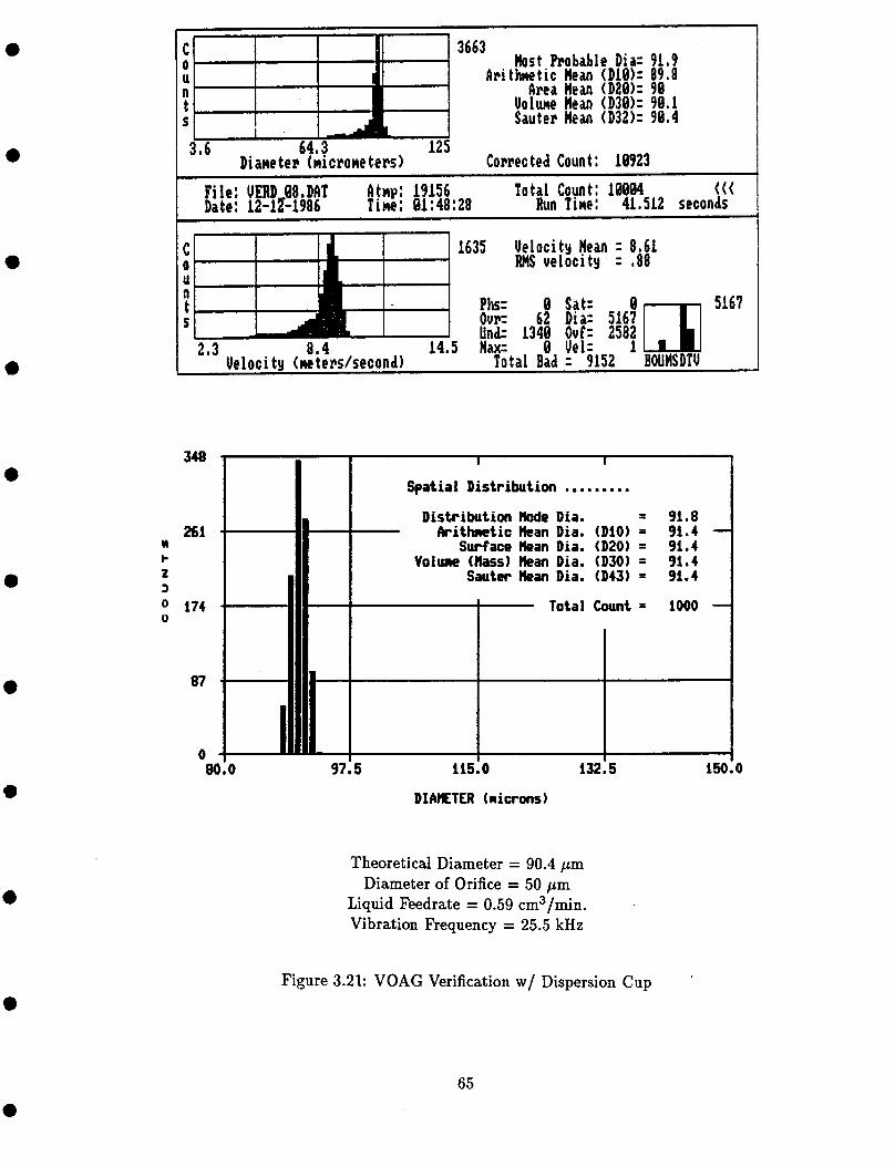
a C U n t . S

0

a

3663 Most Probable Dia: 91,9

Arithmetic Mean (D18)= 89.8 Area Mean (D28): 98

Uolune Mean ( D 3 k 9 8 , l Sauter Mean (D32)= 98,4

a

348'

261 - Y I- 2 3

0 174 -

87 -

0 80.0 97.5

e I I

Spatial Distribution . . . . . . . . Distribution )lode Dia. = 91.8 kithnetic Mean Dia. (DlO) = 91.4 -

Surface Hean Dia. (D20) = 91.4 Volune Mass) Mean Dia. (D30) = 91.4

Swtw Mean Dia. (D43) = 91.4

Total Count = I000 -

115.0 132.5 1%

a

e Theoretical Diameter = 90.4 pm

Diameter of Orifice = 50 pm Liquid Feedrate = 0.59 cm3/min. Vibration Frequency = 25.5 kHz

0

Figure 3.21: VOAG Verification w/ Dispersion Cup a

65

a

332- I I

Spatial Distribution . . . . . . . . . Distribution hde Dia. = 102.4

11 Surface Hean Dia. (020) = 102.0 Volune (Haass) Mean Dia. (D30) = 102.1

z Sauter Mean Dia. (043) = 102.1

249 -' Arithrretic kan Dia. (Diol = 102.0 - c

3

0 166 Total Count = 998 - -'

83 - -

0 - *

90.0 107.5 125.0 142.5 160.0

0

a

a

0

a

2744 Most Probable Dia= 100,7

llri thnetic Mean (Dl0k 98.7 llrea Mean (D20k 99

Volune Mean (D30)= 99.3 Sauter Mean (D32k 99.8

Corrected Count; 10284 File: UERD 09.Dllf l l h p : 11800 Total Count: 10809 ((( I Date: 12-12-1986 Tine: 01:18:28 Run Tine: 126,682 seconds

C 1538 Velocity Mean = 5,94 0 RHS velocity : ,7 n t U

Phs= 0 Sat= 1264 O w 25 Dia= 1261 ml Und= 480 Ouf=

Ueloci tu (Meterdsecond) Total Bad = 1788 BOUMDTU

S

2,3 8 . 4 14.5 Max= 19 Uel= 0




66

a

lee ,

8 0 , n E

aJ 60 - B n

P v

- ra .-

48 -

20 ,

0

a

+ 6 + + A A A rn rn rn rn

P/DPA Arithmetic Menil Diameter TSI Cnlculated Diameter LI/VPS Arithnictic Mean Dianicter

.A.

e l I I I I I I I I I

0 I 2 3 4 6 6 7 0 0 10

Verification Test (#) CASE I

VOAG w/o Dispersion Cup.

,

Figure 3.23: Comparison of Arithmetic Mean Diameters for CASE I VOAG Verification w/o Dispersion Cup Results

67

a

e

a

a

a

128

I80

88

60

4 0

28

8

0 0 0 0 A A A rn rn rn

P/DPA Arithmetic Mean Diameter TS1 Calculated Diameter LI/VPS Arithmetic Mean Diameter

0 1 2 3 4 6 6 7 e 0 le Verification Test (#)

CASE XI VOAG w/ Dispersion Cup.

a Figure 3.24: Comparison of Arithmetic Mean Diameters for CASE I1 VOAG Verification w/ Dis- persion Cup Results

e

68

a

Table 3.4: VOAG Verification Results

CASE I

Vibrating Orifice Aerosol Generator w/o Dispersion Cup.

LI/VPS Results P/DPA Results

ARITHMETIC ARITHMETIC STANDARD

DIAMETER DIAMETERDEVIATION DIAMETER DEVIATION TEST TSI MEAN STANDARD MEAN

(#) (Pm) (Pm) (Pm) (Pm) (P.tm)

1 2 3

19.8 35.5 39.0

19.1 35.9 39.8

0.101 0.8 18 0.047

20.5 35.8 39.6

2.073 1.020 0.060

4 5 6

41.5 44.2 47.5

41.8 43.3 49.2

0.128 0.045 0.076

42.7 45.2 48.8

0.176 0.150 0.153

7 8 9

85.6 90.4 99.6

85.6 91.2

100.3

0.108 0.142 0.340

89.4 90.3 99.9

0.270 0.399 0.436

CASE I1

Vibrating Orifice Aerosol Generator with Dispersion Cup.


ARITHMETIC ARITHMETIC STANDARD

DIAMETER DIAMETER DEVIATION DIAMETER DEVIATION TEST TSI MEAN STANDARD MEAN

(#I (Pm) ( P d (ctm) (Ilm) (m)

1 2 3

19.8 35.5 39.0

19.2 38.3 40.2

0.325 0.432 1.355

21.5 36.8 40.0

2.063 1.560 0.566

4 5 6

41.5 44.2 47.5

43.5 42.7 49.1

1.063 1.109 0.541

41.9 45.5 49.7

0.120 0.379 0.275

7 8 9

85.6 90.4 99.6

86.7 91.4

102.0

0.139 0.175 0.420

86.1 89.8 98.7

2.080 0.844 0.155

a

5 0 - I I

Spatia 1 Distribution . . . . . . . . . Distribution bode Dia. = 6.4

w Surface Mean Dia. (D20) = 10.9 Volure (Hass) Hean Dia. (D30) = 12.4 t

2 Sauter Hean Dia. (032) = 16.4 3

0

SI .' Arithaetic Hean Dia. (Diol = 9.5 -

25 - r Total Count = 500 -

12 -

a

0

a

0

a

a

0

0

,

Host Probable Dia= 7,1 C 649 U Arithrwtic kan (DlW: 12.3 n Lna kan (D28): 13,7 t Volume kan (D38): 15.1 S Sauter kan (D32k 18.3 1.1 28.6

0

Corrected Count: 13878 File: MS4 1 MI htnp: 12258 Total Count: 9569 ((( Date: @-dlk? Tim: 89:59:29 llun Tine: 5.545 seconds

2.4 11.2 28.8 Ueloci tu (mters/second)

364 Velocity ban = 14,52 RI(s velocity : 2.85

Und= la5 Our= Max= 1 Val= 116

Total Bad = 1924 BOUHSDTV

1815

a. P/DPA Results

DIAMETER (aicrons)

' b. LI/VPS Results

(CASE I) Test Conditions: Radial Position = Cr,

Air Pressure = 65 psia Water Pressure = 105 psia

Water Flowrate = 0.038 gal/min. Axial Position from Nozzle = 2 ft.

Figure 3.25: MOD-1 Nozzle Comparison

ONGINAL PAGE IS ZWR QUALITY 70

e

5 0 1 I 1

Spatial Distribution .. ...... . Distribution Mode Dia. f 7.0

u Surface Hean Dia. (020) = 11.2 k Volune Mass) ban Dia. (030) = 12.8 z Sauter Hean Dia. (D32) = 16.5

2 25 * Total Count = 500 -

3 7 - Arithretic Bean Dia. (010) = 9.8 -

- - 2

- 12 -

a

a

a

0

0

Dim ter (ni crow t ers 1

658 h s t Probable Dir: 7,1

Arithmetic lkan (DUN: 12.1

U o t w Rean (D30): 14.9 Sauter llean (0321: 18.2 .

aRr llem (DW 1 ~ 6

Corrected Count: 12298 File: WS4 2 MT h p : 12258 Total Count: 9375 I Date: 08-ddn Time: 18:01:11 h h e : 5,848 seconds

2.4 11.2 . 28, e Ueloci ty (mtem/second)

371 Uelocity Hean : 14.71 RHS velocity : 2.8

Phs= 0 Sat: oVr= 278 Dia= 591 TTT] Und= 1189 Out: b 1 Vel: 122

Total Bad : 2199 BOUHSDTU

1189

-

b. LI/VPS Results (CASE I)

Test Conditions: Radial Position = $ in. Air Pressure = 65 psia

Water Pressure = 105 psia Water Flowrate = 0.038 gal/min. Axial Position from Nozzle = 2 ft.

a

71

a


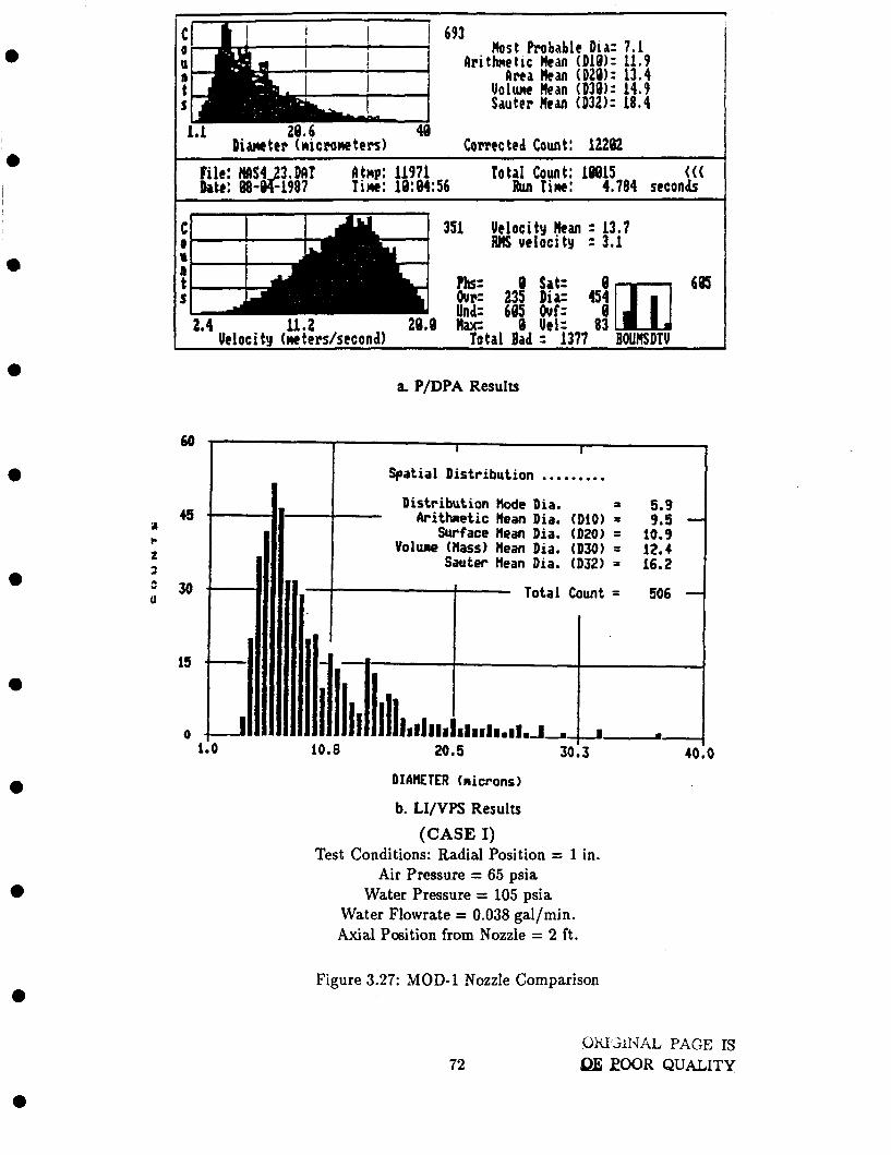
0

6 0 -

45 - a P z -

30 * 0

693 k s t Probable Dia: 7,1

C 0 0 f i r i t h e t i c Hem (Dlfd): 11.9 n Area Hean (D28)= 13.4 t Uolw Hean (D38): 14.9 E Sauter Hean (D32): 18.4 1.1 29.6 49

Diane ter (nicrone t e n ) Corrtcted Count: 12202

I I

Spatial Distribution . . . . . . . . . Distribution node Qia. = 5.9 Arithmetic flean Dia. (DIO) = 9.5 -

Surface Hean Dia. (020) = 10.9 Volwe (Hass) Hean Dia. (D30) = 12.4

Sauter flean Dia. (D32) = 16.2

- Total Count = 506 -

File: MS4 3 DAT Atnp: 11971 Total Count: 18815 ((( I Date: 08-dljal Tim: 18:84:56 Run Tim: 4.784 seconds r

351 Velocity ljean : 13.7 Rlls velocity : 3.1

2.4 11.2 kloci ty (mters/second)

Phs: B Sat: Our: 235 Dia= 451 01 Und= 685 Ouf: Hw- 8 Vel: 83

Total Bad : 1377 BOU6DTU

0 a. P/DPA Results

0

0

a

0

0

605

-

0

0


72 OMl;ll.JhL PAGE IS QE EOOR QUALITY

-- Diamttr (microneterr) Corrected bunt: 13463

31

25 -

12 -

0

File: MAS4 4 DAT Atrrp: 12117 Total Count: 18684 ((( ktr: ~ d k Tim: l0:66:38 Run Tiw: 3,236 seconds

Spatial Distribution ......... Distribution Mode Dia. = 7.0

Surface Hean Dia. (D20) = 11.3 Volune (Mass) Mean Did. (030) = 12.8

Sauter Mean Dia. (D32) = 16.2

*. kithnetic Mean Dia. (DlO) = 10.1 -

Total Count = 503 -

1.0 -I I i 10.8 I ~III,,,,.,,J.,,,J.J-,-J 20.5 ,..-.. 30.3 -.-. 40.0

a

a

a

a

e

b. LI/VPS Results

(CASE I) Test Conditions: Radial Position = If in.



a

73


I I

I llrithwtic Hean (Dl8): 9 , 8 a h a Nean (028): 11.3 t U o l w w Hean (D38): 12.8 3 Surter kan (032): 16.5 1.1 28.6

Diameter (nicroncters) Corrected Count: 12661 File: MS4 5,DAT htnp: 12258 Total Count: 9873 ((( kte : ~-d l~~7 Tim: 18:08:24 Run Tim: 2,716 seconds

a

5 0 - I 1

Spatial Distribution . . ...... . Distribution node Dia. = 6.4

Y Surface Hean Dia. (D20) = 11.1 c Volune (nass) Hean Dia. (030) = 12.6 2 Sauter tiean Dia. (D32) = 16.4 3

0

37 - ' kithattic Haan Dia. (010) = 9.7 -

2 s - Total Count = 500 -

12 1

a

11)11.1..11.1..1111. ...... id.--,

I r i

1 Vcloci ty (mters/second)

a

a

0

a

284 Uelocity &an : 11.06 RMS velocity = 3.49

Und= 617 Our= Ilax= 2 Vel= 16

Sotal Bad = 1779 BOUIISDIU

a. P/DPA Results

876

-

DIAHETER (ricrons)


Test Conditions: Radial Position = 2 in. Air Pressure = 65 psia


0 Figure 3.29: MOD-1 Nozzle Comparison

74

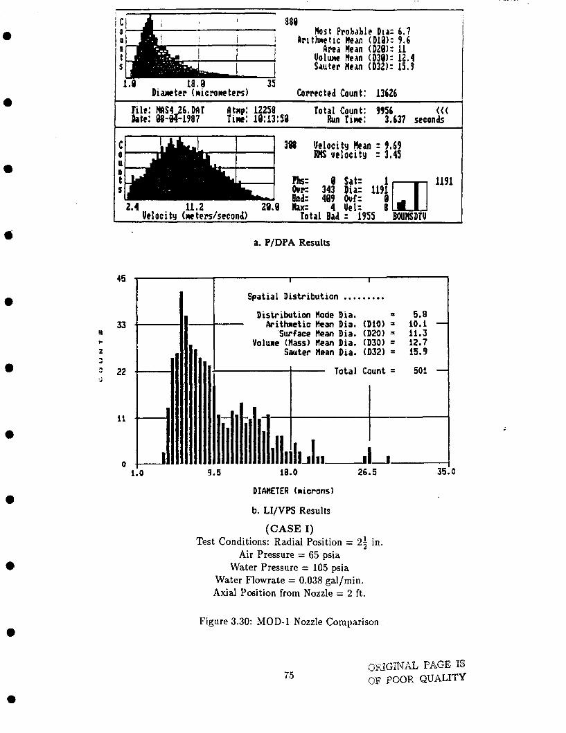
a

Spatial Distribution .. . . . . . .. Distribution node Dia. = 5.8

Arithrctic Mean Dia. (010) = 10.1 - Surface tlean Dia. (D20) = 11.3

Volune (Hass) tlean Dia. (D30) = 12.7 Sauter Hean Dia. (D32) = 15.9

Total Caunt = 501 -

33. IJl

r 2 2

3 22 .. J

11 - '

35.0

e

a

~ ~

880 Host Probable Dia= 6 . 7

llrithrretic Hean (DUN: 9 . 6 brea Hean (D20): 11

Uolune Hean (D38): 12,4 Sauter Hean (D32): 15 .9

Corrected bunt : 13626 Tile: WAS4 6 DAT Atnp: 12258 rota1 Count: 9956 1 k t e : e e - $ l j g l rim: 19:13:50 Run Tim: 3.637 seconds

2.4 11.2 28.0 Ueloci tu (ne terdsecond)

368 Velocity Hean : 9.69 R)Is uelocity : 3.45

Und= 499 Our= Iluc= 4 Vel: 8

Total Bad = 1955 BOUHSDTU

1191

- a. P/DPA Results

45 1 1 1 1

b. LI/VpS Results

(CASE I) Test Conditions: Radial Position = 2 1 in.



Figure 3.30: MOD-1 Nozzle Comparison a

75

a

a

38. I I

Spatial Distribution . . . . . . . . . I Distribution node Dia. = 5.8

a Surface Hean Dia. (D20) = 11.7

t Sauter Hean Dia. (D32) = 16.0

a - Arithnetic !lean Dia. (Diol = 10.5 - r Voluae (Hass) Hean Dia. (030) = 13.0

2

0 19 - Total Count = 500 -

9 - '

I L U A - A A - 0 1.0 p

I 9.5 l l~ l l l l l~ l~ . l , I ,~ 18.0 1 I11J 26 I 5 35.0

a

C 0 I n t I

1.0 35 I Dianeter (ni crone t e n )

811 Host Probable Dia= 6.7 k e a Hean (D20): 10.4

Uolw Hean (D30)= 11.8 Sauter kan (D32): 15,4

Irithmetic Hean (D10): 9

Corrected Count: 12364 Pile: MS4 7 MT Itnp: 12258 Total Count: 9439 ((( Rate: Q8-dlhl Tine: 19: 15:25 Run Sine: 4.877 seconds

C 319 Uelocity Fan : 8.14 0 R)Is velocity : 3.14 a I Our= 4& DIG 1728

2.4 11,2 20,Q k- 11 Uel: 3

0

t p)rs= 8 Sat= LJ 1728 Und= 386 Out:

k l o c i ty (neterslsecond) Total Bad = 2534 BOUNSDTU

a. P/DPA Results

a Figure 3.31: MOD-1 Nozzle Comparison

76

153 Host Probable Dia: 5 . 7

U Arithmetic Hean (Dt8): 8.8 n Area Mean (D28): 18.3 t Volume Hean (D38): 11.9 5 Sauter Nean (D32): 15.7

' c 0

1

18.0 35 Di MC ter (ni c r o ~ t ers 1 Corrected Count: 11488

Spatial Distribution . . . . . . . . Distribution node Dia. = 5.8 Arithnetic Hean Dia. (Diol = 10.7 -

Surface nean Dia. (020) = 12.0 Volure (Hass) nean Dia. (D30) = 13.4

Sauter ?lean Dia. (D32) = 16.7

Total Count = 500

Run Tim: 19.390 seconds File: MS4 8 UT Atnp: 12258 Total Count: 8679 I Date: @-dlh? Tine: 10:16:52

2.1 11.2 2% 0 Ueloci tu (mters/second)

393 Velocity Uean : 6.89 1\)1s velocity = 2.92

Und= 369 Ovf= Ilw= 2 Vel: 6

Total Bad = 3318 BOUHSDTU

2499

a. P/DPA Results

38 T I I I 1

28

19

9

0

I L

1:o

DIAflETER (nicrons)


Test Condtions: Radial Position = 35 in. Air Pressure = 65 psia



1 .

c b,*n~>.G;~1 71-d, >LASE 1s OF POOR QUALITY

77

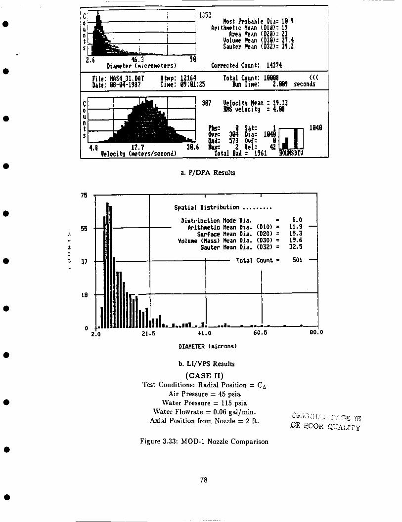
a

e

a

a

a

a

a

a

a

c : A I

D i MC ter (n i crone ters 1

1352 Most Probabl

LIri thrwtic Hean k e a Nean

Uolunr Hean Sauter Hean

Corm ted Cow t :

i

i , e Did: 18 ,9 (DlQ)= 19 (D28)= 23 (038): 27.4 (032): 39 ,2

14374 File: MS4 31.MT Atmp: 12164 Total Count: lW ((( Date: 08-Q?-1987 Tint: 09:81:25 Run Tine: 2.889 seconds

C

n t 5

0 U

- 4.8 17.7 30,6

Ueloci ty (me terdsecond)

387 Velocity Rean : 19.13 IUS velocity : 4,98

Unci= 573 Ouf: k 2 Vel: 42

Total Bad z 1961 BOUIISDTU

Pk B Our= 384 Unci= 573 k 2

Total Bad

Dia: 1640 Sat= Ouf: Vel: 42 z 1961 BOUIISDTU

:m a. P/DPA Results

1048

I 1 I 1 Spatial Distribution . . . . . . . . .

Distribution Mode Dia. = 6.0 Arithaetic Mean Dia. (DlO) = 11.9

Surface Mean Dia. (D20) = 15.3 Voluae (Hass) tlean Dia. (D30) = 19.6 -+ Sauter Hean Dia. (032) = 32.5

2i.5 41.0 60.5 80.0

DIAnETER (ricrons)

b. LI/VpS Results

(CASE 11) Test Conditions: Radial Position = Cr,



L?,aY!'>. ;dl;L : ;.?E lrr

DE %mix Q'WA&pf


78

a

a

80 1

0

1 I 1 1

e

60 IA

t :

0

c

40

20

0 2.0

0

a-

a-

-- I

--

e

Spatial Distribution ......... Distribution Mode Dia. = 7.2 Arithretic tlean Dia. (DlO) = 12.3 -

Surface Hean Dia. (D20) = 16.2 Volune (Hass) Hean Dia. (D30) = 21.0

Sauter tlean Dia. (D32) = 35.5

Total Count = 500 -

I ~ DiaMter (micrometers)

I. lill,ll,~l-d-a-.*.~A 21.5 41.0 -I---- 60.5 -I.-- 80.0 -

1072 Host Probdde h a = 18.8

Arithrrctic tiean (010): 18.3 a r t i HeAn (028): 22.1

U o l w tiedn (D30): 26.2 Sauter flew (D32): 36.8

Corrected Count : 13318

Pile: MS4 32.08T Atnp: 12258 Total Count: 9796 ((( I 1 Date: 88-9?-1987 Tim: 89:84:43 Run Tine: 2.816 seconds I , 1

4.8 17.7 Ueloci ty Ineters/second)

352 Uelocity kan : 18.5 M velocity : 4.19

Und= 744 Out: Hax: 6 Vel: 19

Total Bad : 2222 BOUSDTU

a. P/DPA Resulk

1164 1

DIAHLTER (nicronr 1

b. LI/VPS Results

(CASE 11) Test Conditions: Radial Position = !j in.




79

e

e

e

e

0

e

0

0 U n t 5

2.3 ~ 41.1 ae Dianeter (nicrom ters)

1292 Host Probable Dia: 8.5

Arithmetic Hedn ( D L W : 16.2 Area k a n (D28): 19.3

Uolwe &an (038) : 22,8 Sauter flean (032): 31.7

Q m c t e d Count: 13958 File: MS4 33.MT Atnp: 12258 Total Count: 95W ((( 1 Date: W-84-1987 Tim: 69:67:31 Run Tine: 2.226 seconds

4.8 17.7 Urloci tu (mterdsecond)

388 Uelocity Mean : 16.74 Riff velocity : 4.13

P ~ S = e Our= 381 Und= 651 M ; u c = 5

Total Bad

a. P/DPA Results

Sat=

Vel: 4 = 2561 BOUHSDTU

5s -- u I= 2 J

i) O 37 --

18 a-

0 - 2.0

I I

Spatial Distribution . . . . . . . . . Distribution node Dia. = 7.2 Arithaetic Mean Dia. (DlO) = 11.8 -

Surface ttean Dia. (D20) = 14.8 Voluae (Hass) nean Dia. (D30) = 19.0

Sauter nean Dia. (D32) = 31.3

Total Count = 500 -

I,,, 1.111 _1.1..1_144-4 41.0 I .,A. 60.5 __-- 80.0 21.5

DIAHETER (ricrons 1

b. LI/VPS Results (CASE 11)

Test Conditions: Radial Position = 1 in. Air Pressure = 45 psia

Water Pressure = 115 psia Water Flowrate = 0.06 gal/min.

Axial Position from Nozzle = 2 ft.


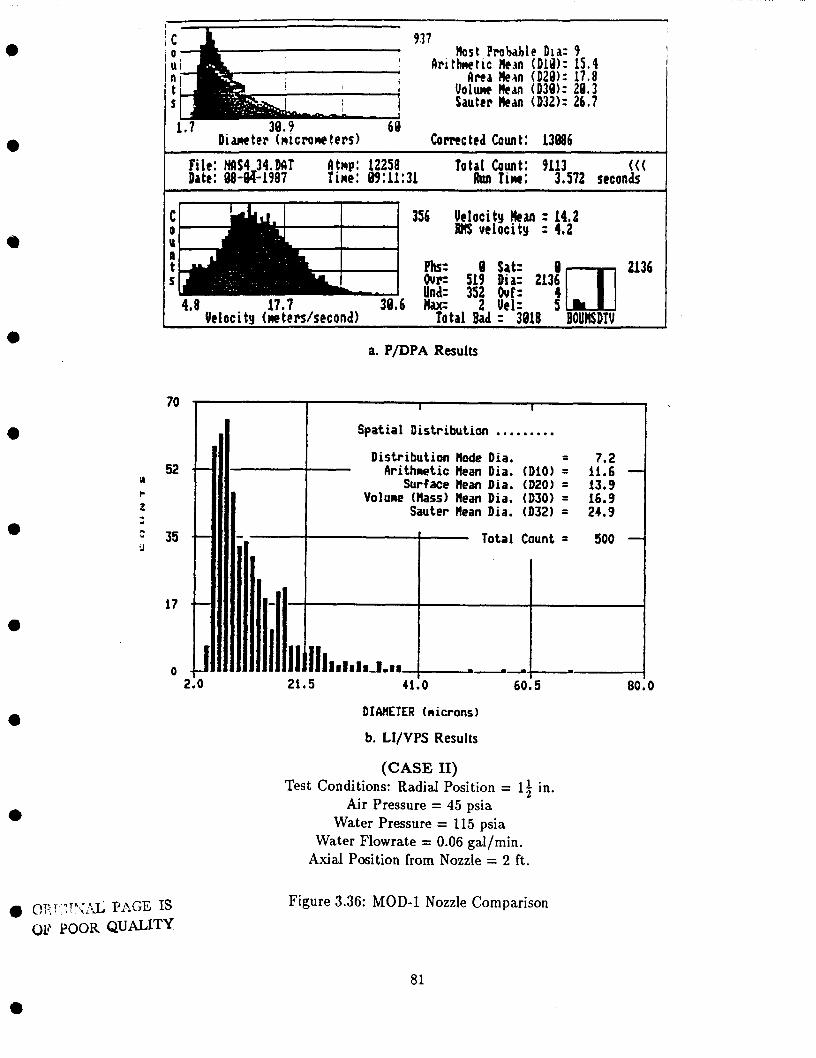
0

I I

Spatial Distribution . . . . . . . . . Distribution Hode Dia. = 7.2 Arithaetic Hean Dia. (DlO) = 11.6 -

Surface Hem Dia. (D20) = 13.9 Voluae (Ilass) Hean Dia. (D30) = 16.9

Sauter Hean Dia. (D32) = 24.9

Total Count = 500 -

l~ldm-l.~a I)-- -

41.0 60.5 80.0 I- a l l 21.5 1 Ill

0

0

0

0

e

0

! 937

Host Probable Dia: 9 Arithmetic !em (Did): 15.4

n fired Hean (020): 17.8 t U o l w kan (D39): 29.3 S Sauter Hean (D32k 26.7

: C \

I O U

39.9 60 Diane ter (ni crow ters) Comc ted Count : 13886

File: MS4 34.01'1 fltnp: 12258 Total Count: 9113 ((( Date: 08-g-1987 Tine: 09:11:31 Run Tim: 3.572 seconds

~~ ~

C 356 Velocity ban : 14.2 0 R?lS velocity : 4.2 n I Ovr= 519 Dia: 2136

4.8 17.7 39.6 Ilax= 2 Vel= 5

U

t PIE= e s+t= :Dl 2136 Und: 352 Ouf=

Veloci ty (mters/second) Total Bad = 3018 BOUHSDTU

70

52 u I- t . d

35 0

17

0 2

a. P/DPA Results

DIAHETER (nicrons)

b. LI/VPS Results

(CASE XI) Test Conditions: Radial Position = 1; in.




81

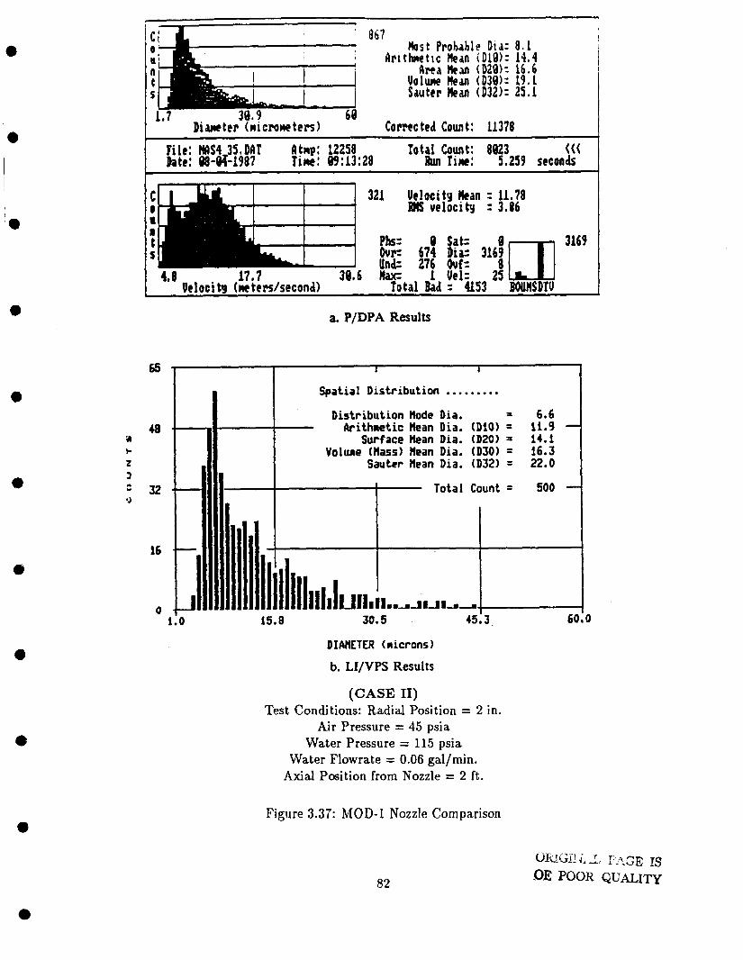
a

6 5 - I I

Spatial Distribution ......... Distribution node Dia. = 6.6

a Surface Hean Dia. (D20) = 14.1 I- Volume (tlass) tlean Dia. (D30) = 16.3 z Sauter nean Dia. (D32) = 22.0

E 32.- 1 Total Count = 500 -

48. bithmetic Hean Dia. (Diol = 11.9 -

3

3

16

a

I

a

0

e

a67 host Probable Did: 8 . 1

C P Arithmetic Nea iDlW: 14.4 n Area Hem (D28): 16.6 t V o l u t e Rem (D38): 19 .1 5 Sauter Man (D32k 25,l

0

Diamter (microwe t e n ) Cometed Count: 11318 ~

Pile: WAS4 35,DllT Atup: 12258 rota1 cow: ~3 ((( Date: 08-0?-1987 Tim: 89:13:28 h rim: 5.259 seconds

4.8 1?,7 Ueloci ty (mters/second)

321 Velocity ban : 11.78 RllS velocity = 3.86

Und: 216 Ouf= k 1 Vel: 25

Total Bad z 4153 BOUNSDTU

3169

a. P/DPA Results

(CASE 11) Test Conditions: Radial Position = 2 in.




82

0

45 a b 2 3

r) 30.-

814 I

Ilrithmetic Hetn (D18): 14.1 I h s t Probable Dia= 8 . 1

k e a Hean (D28)= 1 6 . 3 Uollulrc Hean (D30): 18,7 Sauter Mean (D32): 24,7

1.7 38a9 60 Diamtcr (nicroneters) Corrected Count: 9813

Spatial Distribution . .. .. . .. . Distribution node Dia. = 5.8 Arithnetic Mean Dia. (DlO) = 12.7 -

Surface Hean Dia. (DZO) = 14.7 Yolure (Hass) Hean Dia. (D30) = 16.8


Total Count = 500 -

File: MS4 36,Dflr htmp: 12258 Total Count: 7225 I Date: 88-M-19e7 r i m : 89:15:26 Run Tim: 18.796 seconds

m,mI m-m I l5 0 1.0 -,I h 1)1 15.8 l-ill~,Il,,~*,,B.,~,~B 30.5 45.3 60.0

l

I 4.8 14.9 25.0 Ueloci tu (neterdsecond)

388 Velocity kan : 9.72 Rlls velocity : 3 . 3

Phs: 8 Sat: 2: nl Our= 882 Dia: 3853

Und= 235 Ouf: n;uC= 1 Uel: 62

Total 'Bad : 4973 BOURSDTU e

a. P/DPA Results

0

a

e

0

3853

-

60 I I I 1

DIAHETER (aicronc)

b. LI/VPS Results

(CASE 11) Test Conditions: Radial Position = 2; in.



0

0


83

a

45 * 111 k z 3 * 30 J

15

0 1.0

e

Spatial Distribution ......... Distribution node Dia. f 4.9 Arithretic Hean Dia. (010) = 12.4 -

Surface Hean Dia. (020) = 14.4 Volune (flass) Hean Dia. (D30) = 16.3


a- Total Count = 500 -

a-

r' I 1,1~,,,~l,,l,,,.,,",3 15.8 30.5 .,I. 3. 45.3 60.0

-

a

-. .

Diane ter (ni crone terr 1

- 878

Host Probable Dia: 8 . 1 hi thnetic Mean CDlQ): 14.6

k e a Hem (D28): 16.6 Uoliulc Hean (D38): 18,9 Sauter kan (D32): 24,4

Corrected Count: 19935 Pile: M54 37.DAT Atmp: 12258 Total Count: 7821 ((( Date: @-M-1987 Tine: 89:17:91 Run Tim: 21.969 seconds

491 Uelocity Hean : 9.88 Riff velocity : 3.01

c

a

Our= 967 Dia: 3141 t Phs: 8 Sat:

Und= 128 Out: 4.8 14.9 25,0 Hax= 6 Vel: 184

0 U

6:ni 31u 3

Ueloci ty (mterslsecond) Total Bad = 4394 BOUHSDTU

a. P/DPA Results

60 I I I I

DIAMTER (nicrons) b. LI/VPS Results

(CASE 11) Test Conditions: Radial Position = 3 in.



84


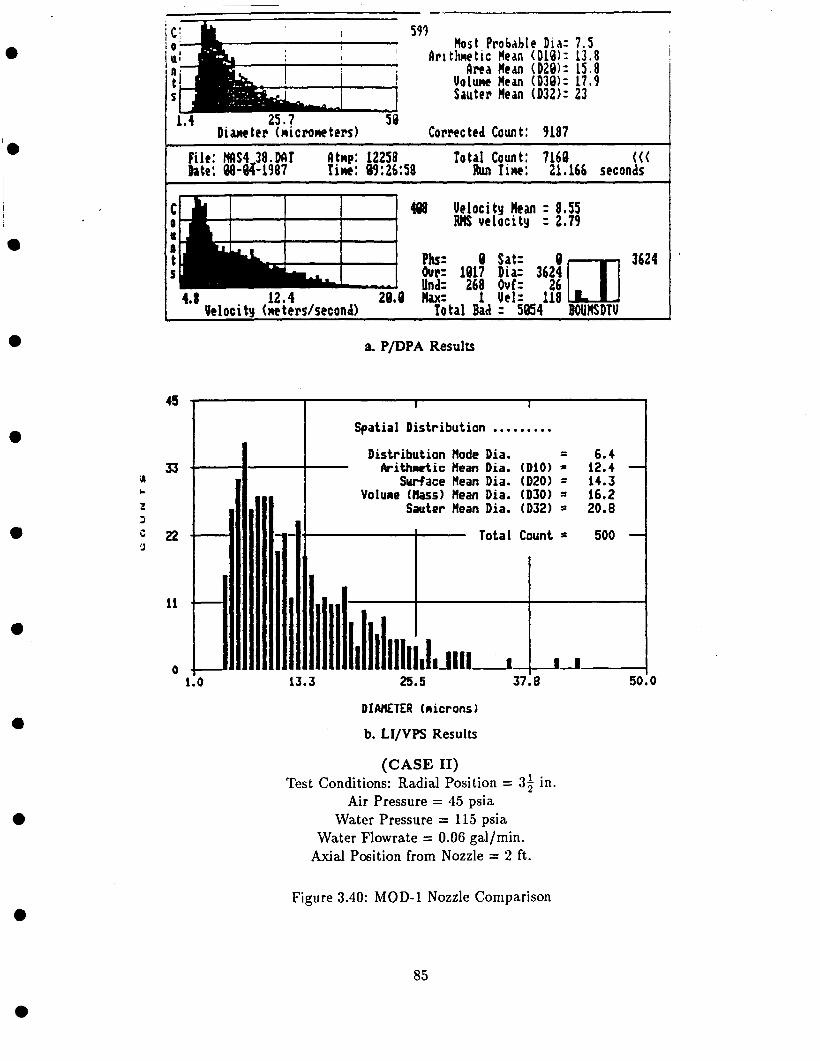
e

' File: MS4 38.DAT Btnp: 12258 Total Count: 7168 ((( Date: aS-$%1987 Tim: 89:26:58 Run Tine: 21.166 seconds

C 498 Velocity Ran = 8.55 RllS velocity : 2.79 0

U R

I t PhS: 8 Sat= 2: nj 3624 5 Our= 1817 Dia= 3624

4.8 12 .4 29.0 Hax= 1 Uel: 118 I Ocloci tu (mters/second) Total Bad : 5854 BOUHSDTU

Una: 268 out=

33 k 0 Spatial Distribution . . . . . . . . . Distribution tlode Dia. = 6.4 Arithnetic tlean Dia. (DlO) = 12.4 -

Surface tlean Dia. (D20) = 14.3

0

e

599 host Probable Did=

bri t h e t i c Nean CDl@)= Brea Hem (D28):

Volume Hcan (030)= Sauter Wean (D32):

Corrected Count: 9187

a. P/DPA Results

45 1 1 I 1

Volune (&ss) tlean Dia. (D30) = 16.2 Sauter Hean Dia. (D32) = 20.8

22 Total Count = 500 -

J

11

0 13.3 25.5 3718 5a

DIMETER (nicrons)

' b. LI/VPS Results

(CASE 11) Test Conditions: Radial Position = 3; in.



0

0

85


‘0

0

a

0

e

To study the aforementioned results, the arithmetic mean diameter and Sauter mean diameter from each test were graphed as functions of radial position (Figs. 3.41 and 3.44) for each case. The choice of the arithmetic and Sauter mean diameters in the graphs was made to examine the count vs. particle size distribution. The distribution shape most associated with aerosol spray analysis is similar to a log-normal distribution where the distribution mode leans toward the low side of the distribution and conversely the distribution tail.shifts to the high side of the distribution. The distribution is reproduced by the fact, that the arithmetic mean diameter is proportional to the mode of the distribution and the Sauter mean diameter is indicative of the distribution’s tail. With the above technique, the comparison of results from the P/DPA and the LI/VPS was performed.

3.2.1

Referring to Table 3.5, the arithmetic mean diameters measured by the LI/VPS remained approximately constant from 9.5 pm at the centerline to 10.7 pm at the edge of the spray, while the P/DPA values varied from 12.3 pm at the centerline to 8.8 pm at the edge of the spray. Figure 3.41 shows the general trend in the LI/VPS and P/DPA arithmetic mean diameter to be very similar with a maximum deviation of 2.8 pm at the centerline and a minimum deviation of 0.1 pm at the 2.0 inch location. Figure 3.42 shows the trend in the Sauter mean diameter to be also similar for both instruments. The maximum deviation is 2.2 pm at the 1.0 inch radial position while the minimum deviation is 0.0 for the 2.5 inch position. The maximum deviation of 2.8 pm for the arithmetic mean diameter, and 2.2 pm for the Sauter mean diameter can be explained as a result of the difference in instrument operation (automatic imaging vs light scattering and spatial vs temporal), the depth of field correction used by the P/DPA and no correction for the LI/VPS system, and to the LI/VPS instrument calibration error calculated to be f 2.6 pm with a standard deviation o f f 2.0 pm.

Discussion of Results for Comparison - CASE I

3.2.2

Referring to Fig. 3.43 and Table 3.5, the maximum deviation in arithmetic mean diameter of 7.1 pm occurred at the centerline with the minimum deviation of 1.4 pm at the edge of the spray. As in CASE I, the LI/VPS arithmetic mean diameters remained approximately constant from 11.9 pm at the centerline to 12.4 pm at the edge of the spray, and the P/DPA values varied from 19.0 iim at the centerline to 13.8 pm at the outer edge. Figure 3.44 showed a very similar trend in Sauter mean diameters as a function of the radial location for both instruments. A maximum deviation of 6.7 pm occurred at the centerline of the spray and a minimum deviation of 0.4 pm at the 1.0 inch location.

In CASE 11, the increase in water pressure may increase the turbulence in the outer region of the spray plume, which in turn caused recirculation of particles through the overlapping probe volumes. In addition to the explanations given in CASE I for the the differences in the arithmetic mean diameters we believe that since the trend for both cases is very similar (Le., LI/VPS values remained approximately constant across the spray plume, while the P/DPA values decreased as the measurements approached the outer edge of the spray), some of the differences is due to the more difficult test conditions of CASE 11. As we approach the outer edge of the spray, there is better agreement in the arithmetic mean diameter for both instruments. A possible explanation is the way the P/DPA operates. Recalling from Section 2.1, for proper operation of the P/DPA, the drops must pass through the probe volume perpendicular to Doppler fringes. Drops exactly at the centerline of the spray will almost always be perpendicular to these fringes and as we approach

Discussion of Results for Comparison - CASE I1

86

a

the outer edge, the drops at these locations will have different directions. The result is an increase in run time which for CASE I1 varies from 2.0 sec at the centerline to 21.2 sec at the edge of the spray. The increase in time is an indication that more particles were rejected; therefore, the system becomes more selective and perhaps explains the smaller arithmetic mean diameter as the edge of the spray is approached. The difference in arithmetic mean diameters in the inner region of the spray is attributed to the loss of small particles due to the presence of high number of liquid particles per volume of air which produces overlapping signals in the P/DPA. The number density at the center of the spray was 6970 particles/cm3 compared to 1070 particles/cm3 at the edge. According to Dodge et al[22], by comparing the AMD with the SMD for each case, the differences in the shape of the distribution can be observed. Studying Figures 3.41, 3.42, 3.43, and 3.44 it is observed that the Sauter mean diameter compared more closely than the arithmetic mean diameter which suggests a difference in distribution shape for each case.

a

87

e

30

25 a

e 15 E

Y

L Q) 4

d 10

5

0

a

0

A A

0 0

A A A 0 0 0 0

P/DPA Arithmetic Mean Diameter LI/VPS Arithmetic Mean Diameter

A

0 B 0 U

A A

0 0 . s 1 I .5 2 2.5 3 3.5

Radial Position (inches) (CASE I)

Air Pressure = 65 psia. Water Pressure = 105 psia.

Water Flow-rate = 0.069 gal/min.

Test Conditions:

Figwe 3.41: Comparison of Arithmetic Mean Diameters for MOD-1 Nozzle Comparison Test - CASE I

88

a

e

2 0 L L) .rr c -c

c Q, r) 0) E e Q I-L

0

0

a

30

25

2a

15

10

5

8

A

0

A 0

A 0 0 0 B A

A A A 0 0 0

PfDPA Sauter Mean Diameter LI/VPS Sauter Mean Diameter

I 1 I I I I I I 0 8.5 I I .5 2 2.5 3 3.5 4

Radial Poeltlon (Inches)

(CASE I)



Test Conditions:

Figure 3.42: Comparison of Sauter Mean Diameters for MOD-1 Nozzle Comparison Test - CASE I

a

89

e

38

25

0

28 n

u)

c c) .I

E ! 5 Y

L Q3 3

d a

10 B .I

a

0

a

A A A 0 0 0 0

P/DPA Arithmetic Mean Diameter LI/VPS Arithmetic Mean Diameter

A

A

0 0

A A

0 0

A

0

A 0

A 0

0 8.5 1 1.5 2 2.5 3 3.5 4 Radial Position (inches)

(CASE 11)



Test Conditions:

Figure 3.43: Comparison of Arithmetic Mean Diameters for MOD-1 Nozzle Comparison Test - CASE I1

e

90

a

a

0

0

a

0

0

A

cn E

U

E

2 .d - L Q, 4 Q) E e .r(

P

50

40

a

20

10

0

A A A 0 0 0 0

P/DPA Sauter Mean Diameter LI/VPS Sauter Mean Diameter

A

0

A 0

A 0

A

0

LI

0

A

0 A 0

I I 1 I I I I I 0 0.5 1 1.5 2 2.5 3 3.5 4

Radial Poeitton (inches) (CASE 11)



Test Conditions:

Figure 3.44: Comparison of Sauter Mean Diameters for MOD-1 Nozzle Comparison Test - CASE I1

91

e

a

a

0

e

a

e

Table 3.5: MOD-1 Nozzle Comparison Results

CASE I

Water Pressure = 105 psia Air Pressure = 65 psia


RADIAL ARITHMETIC SAUTER ARITHMETIC SAUTER POSITION MEAN MEAN MEAN MEAN

DIAMETER DIAMETER DIAMETER DIAMETER (inches) (Pm) (Itm) (Pm) (Pm)

CL 0.5 1 .o 1.5 2.0 2.5 3 .O 3.5

9.5 9.8 9.5

10.1 9.7

10.1 10.5 10.7

16.4 16.5 16.2 16.2 16.4 15.9 16.0 16.7

12.3 12.1 11.9 10.8 9.8 9.6 9.0 8.8

18.3 18.2 18.4 17.2 16.5 15.9 15.4 15.7

CASE XI

Water Pressure = 115 psia Air Pressure = 45 psia


RADIAL ARITHMETIC SAUTER ARITHMETIC SAUTER POSITION MEAN MEAN MEAN MEAN

DIAMETER DIAMETER DIAMETER DI A M ETE R (inches) (Itm) (Pm) (P)

CL 0.5 1 .o 1.5 2.0 2.5 3.0 3.5

11.9 12.3 11.8 11.6 11.9 12.7 12.4 12.4

32.5 35.5 31.3 24.9 22.0 21.9 20.8 20.8

~

19.0 18.3 16.2 15.4 14.4 14.1 14.6 13.8

39.2 36.8 31.7 26.7 25.1 24.7 24.4 23.0

92

e

e

a

Section 4

CONCLUSIONS AND RECOMMENDATIONS

This section presents the conclusions of the experimental findings and suggestions for utilizing the experimental apparatus and drop-sizing instrumentation in future studies. The first section deals with the revisions to the LI/VPS, including the upgrade to dynamic particle sizing, the development of the calibration procedure, and the software updates. The second section deals with the comparison of the LI/VPS and the P/DPA, and observations concerning their proper operation, set-up, and limitations. The final section of pertains to the improvement of the LI/VPS to a more complete drop-sizing instrument, the continuation of aerosol spray analysis on the MOD-1 nozzle, and general observations concerning the continuing work in aerosol drop-sizing.

4.1 LI/VPS

The LI/VPS has been upgraded to a system capable of performing drop-sizing analysis on dynamic particles. With the addition of the AD/DA converter board to the control computer, the PSP has shown the capability to distinguish drop-size and focus on dynamic particles in the SPM (Le., freeze frame analysis). Therefore, the LI/VPS’ drop-sizing method and focus criteria, developed prior to this work, remains essentially intact with minor modifications.

A twedimensional calibration procedure for LI/VPS has been developed which allows for a straight-forward, step-by-step process in determining the micron/pixel correction factors associated with the lens magnification and camera tube non- linearities. With the developed calibration procedure and the availability of a f/8 lens (Le., approximate LI/VPS magnification of lOOO), the lower-limit on the measurable, focus- dependent size-span of the LI/VPS has been reduced from 9 pm to 3 pm.

Included in the LI/VPS upgrade has been the development of the PSP set-up sub-program and a drop-size distribution graphics display package. Due to the variability of conditions in aerosol spray analysis and the flexibility of the LI/VPS, the set-up sub- program was developed to aid the operator in his decision process and allow for utilization of the full capabilities of the LI/VPS. The addition of the graphic package was necessary to further the LI/VPS’ ability to characterize aerosol sprays. The graphical representation of the drop-size data was used as a diagnostic tool in specifying the proper drop-size range and a tool in the comparison of the LI/VPS and the P/DPA.

4.2 LI/VPS and P/DPA Comparison

The LI/VPS and the P/DPA compared favorably in the tests performed on the VOAG as well as tests performed on the MOD-1 nozzle. Assuming count vs. drop-size distributions were Gaussian in shape, the monodisperse drops generated by the VOAG, with and without the dispersion cup,

93

a

0

were accurately measured by LI/VPS and the P/DPA within f 2.6 pm. The standard deviation of the test samples were all under 2.0 pm which implies the LI/VPS and the P/DPA probe volumes are consistent in size and boundaries. The MOD-1 nozzle tests also showed similar results for both instruments. Results from CASE I shows substantial agreement in the trend of AMD and SMD values from instrument to instrument with a maximum deviation of 2.8 pm for the AMD,and 2.2 pm for the SMD. In CASE 11, the AMD values determined for CASE 11 show a higher deviation than CASE I (7.1 pm and 2.8 pm respectively). The AMD values agree quite well for the outer region of the spray where the system becomes more selective as explained in section 3.3.2. The SMD for both instruments follows the same trend across the spray with a maximum deviation of 6.7 pm. In icing studies, as well as in combustion and in many other areas, the most important and used diameter is the SMD. Considering the differences in sizing methods employed by the two instruments and the given test conditions, the LI/VPS and the P/DPA comparative measurements were surprisingly close especially for the SMD.

Proper operation and set-up of the LI/VPS and the P/DPA depend on the operating conditions of the tested nozzle or device. For this discussion, the MOD-1 nozzle will be considered. The operating conditions of the MOD-1 nozzle for the aforementioned cases, were not ideal for either instrument. Due to the limited size span available to the LI/VPS, the AMD values determined in CASE I may be slightly higher than the actual values. Considering the turbulent nature of the spray in the outer regions, the P/DPA started to reject counts when collecting data. Therefore, each instrument’s capabilities must be tested a priori in any unknown aerosol spray conditions. Even though the LI/VPS and the P/DPA compared very well and have similar probe volume size, each instrument performs better under different test conditions. The LI/VPS performs well in a high density aerosol spray, whereas the P/DPA under similar conditions, has difficulties due to the overlap of signals or loss of dead-time between signal on the PMTs. The P/DPA has a greater overall size span than the LI/VPS which allows for more versatility. Also, the P/DPA is capable of making velocity measurements concurrently with the drop-size measurement, but as is shown for the MOD-1 comparison, the recirculation of drops associated with the turbulent spray resulted in numerous rejections.

4.3 Suggestions and Recommendation for Future Work

0

The LI/VPS, as particle sizing instrument, has progressed in stages of development. The next stage of development should be in the area of off-line analysis (e.g., frame storage on the laser disk recorder), as well as increasing the program speed through hardware and software modifications. A study should be performed to determine the feasibility of frame storage, and if necessary, the error associated with such storage. The control computer, the behavior of imaging laser, and the PSP program structure should be studied to increase the operating speed of the LI/VPS. With the addition of the Micro-VAX computer, the control computer should not be the limiting parameter in program speed. The PSP trigger to the imaging laser doesn’t function consistently which makes it necessary to check for appropriate background level before processing. Therefore, with proper operation of the imaging trigger, unnecessary processing time can be avoided. Finally, to increase the speed of the LI/VPS, the PSP should be stream-lined. For example, the double-threshold used to determine BGL parameter for particle focus should be consolidated into a single threshold.

The research on the MOD-1 nozzle and the comparison of the LI/VPS and the P/DPA should be continued. Operating conditions for the current work were specified by NASA. Future work on the MOD-1 nozzle should involve tests performed at lower water and air nozzle pressures. These

94

operating conditions would produce a larger drop-size and reduce turbulence in the spray. Also, a position closer to the nozzle would produce a higher number density spray which would be ideal for the LI/VPS. The use of the P/DPA 200 mm transmitter lens would reduce the probe volume which, in turn, would reduce the probability of multiple particles in the probe volume produced by the high number density of droplets. The above suggestions are included to improve the functionality of the two instruments in future studies.

The current research and other comparison work by Dodge et al. I221 and Jackson et al. [23] improve the understanding of the various types of sizing techniques and assist in the development of accurate sizing instrumentation. The selection of a calibration/verification method or standard should be found for all drop-sizing instruments. The selection should be a priority for researchers and instrument manufacturers.

95

a

a

Section 5

REFERENCES

a

0

a

a

a

a

0

1. Proceedings - Particle Sizing Instrument Development Group, 1986 Droplet Technology Work- shop, NASA Lewis Research Center, Cleveland, Ohio, May 1986.

2. Malvern Instruments Limited, Malvern Worcestershire WR14 lAQ, England.

3. Bachalo, W. D., “Method for Measuring the Size and Velocity of Spheres by Dual- Beam Light-Scatter Interferometry,” Applied Optics, Vol. 19, 1980.

4. Bachalo, W. D., and Houser, M. J., “Development of the Phase/Doppler Spray Analyzer for Liquid Drop Size and Velocity Characterizations,” AIAA/SAE/ASME 20th Joint Propulsion Conference, Cincinnati, Ohio, AIAA paper No. 841199, June 1984.

Interferometer,” Applied Optics, Vol. 11, No. 11, 1972.

6. Alexander, D. R., and Morrison, M. J., “Particle Concentration Measurements by Laser Imaging for a Turbulent Dispersion,” Particulate Science and Technology, Vol. 2, No. 4, p. 379, 1984.

5. Farmer, W. M., “Measurement of Particle Size, Number Density, and Velocity Using a Laser

7. Ahlers, K. D., “A Microcomputer-Based Digital Image Processing System Developed to Count and Size Laser-Generated Small Particle Images,” M.S. Thesis, Mechanical Engineer- ing Dept., University of Nebraska-Lincoln, 1984.

8. Alexander, D. R., and Ahlers, K. D., “A Microcomputer- Based Digital Image Processing System Developed to Count and Size Laser-Generated Small Particle Images,” Optical En- gineering, Vol. 24, No. 6, p. 1060, 1985.

9. Ahlers, K. D., and Alexander, D. R., “A Flexible High- Speed Digital Image Processing System, ” SPIE 29th Annual Meeting, Paper No. 573-11, SPIE Proceedings, Vol. 573, San Diego, CA, 1985.

10. Wiles, K. J., “Development of a System for Secondary Liquid Injection into a Mach 2 Super- sonic Flow to Study Drop Size and Distribution by Video Imaging Techniques,” M.S. Thesis, Mechanical Engineering Dept., University of Nebraska-Lincoln, 1985.

Automated Optical Imaging System,” Optical Engineering, Vol. 23, No. 5, 1984. 11. Weiss, B. A., Derov, P., DeBiase, D., Simmons, H. C., “Fluid Particle Sizing Using a Fully

12. Hirleman, E. D., “On-Line Calibration Technique for Laser Diffraction Droplet Sizing Instru- ments,” ASME paper No. 83-GT-232, 1983.

96

a

0

13. Tishkoff, J. M., “Spray Characterization: Practices and Requirements,” Optical Engineering, Vol. 23, No. 5, 1984.

14. Alexander, D. R., Wiles, K. J., Schaub, S. A., Seeman, M. P., “Effects of Non-spherical Drops 1. I

I on a Phase Doppler Spray Analyzer,” Proceedings of SPIE - The International Society of I Optical Engineering, Volume 573, August 21, 1985.

15. ASTM Standard E799-81 (1981).

16. Supplied by NASA Lewis Research Center. a

0

e

a

0

0

e

0

17. Berglund, R. N., and Liu, B. Y. H., “Generation of Monodisperse Aerosol Standards,” Envi- ronmental Science and Technology, Vol. 7,1973.

18. Available from TSI Inc., St. Paul, MN.

19. Bachalo, W. D., and Houser, M. J., “Phase/Doppler Particle Analyzer Operations Manual,” Aerometrics Inc., Mountain View, CA., Release 1.0, 1985.

20. Interview, Bachalo, W. D., Concerning PMT voltage gain voltage, Dec. 9, 1985.

21. Bachalo, W. D., and Houser, M. J., “Measurements of Drop Dynamics and Mass Flux in Sprays,” Presented, 1986 Meeting of the Central States Section/The Combustion Institute, NASA Lewis Space Center, Cleveland, Ohio, May, 1986.

22. Dodge, L. G., Rhodes, D. J., and Reitz, R. D., “Comparison of Drop-size Measurement Techniques in Fuel Sprays: Malvern Laser-Diffraction and Aerometrics Phase/Doppler ,” Pre- sented, 1986 Meeting of the Central States Section/The combustion Institute, NASA Lewis Space Center, Cleveland;Ohio, May, 1986.

Jackson, T. A., and Samuelson, G. S., “An Evaluation of the Performance of Visibil- ity/Intensity Validation and Phase/Doppler Techniques in Characterizing the Spray of an Air- Assist Nozzle,” Presented, 1986 Meeting of the Central States Section/The Combustion Institute, NASA Lewis Space Center, Cleveland, Ohio, May, 1986.

23.

97

e

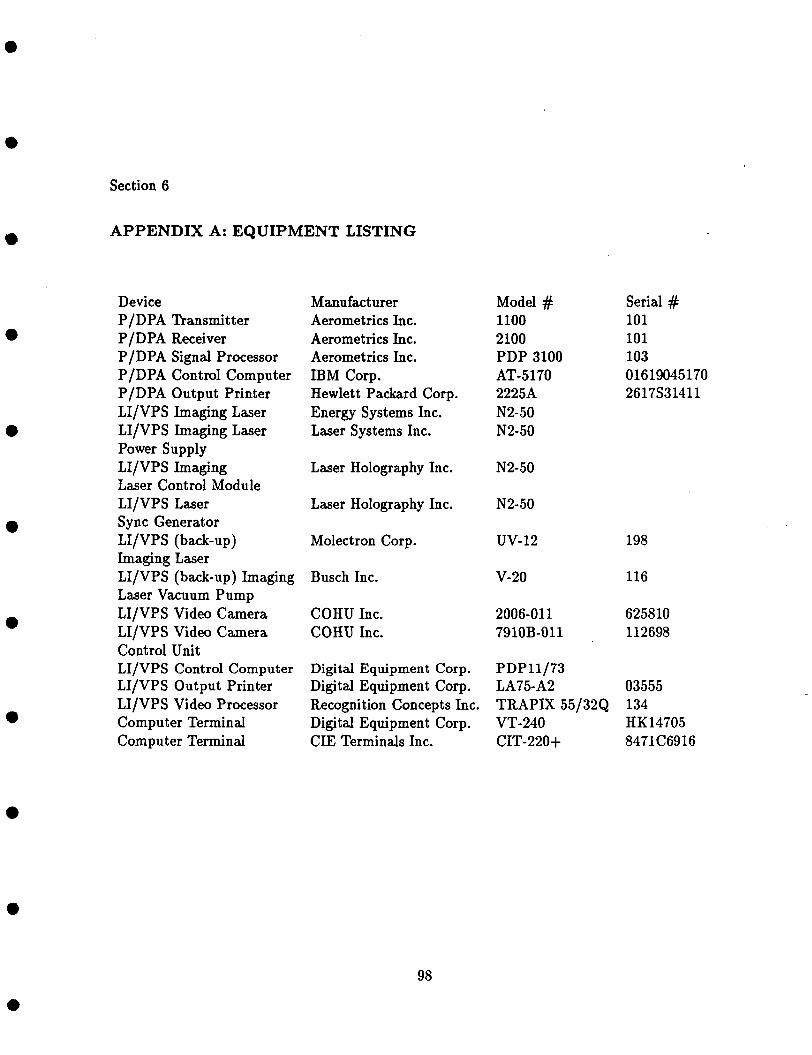
0

0

Section 6

e

a

0

e

a

APPENDIX A: EQUIPMENT LISTING

Device P/DPA Transmitter P/DPA Receiver P/DPA Signal Processor P/DPA Control Computer P/DPA Output Printer LI/VPS Imaging Laser LI/VPS Imaging Laser Power Supply LI/VPS Imaging Laser Control Module LI/VPS Laser Sync Generator LI/VPS (back-up) Imaging Laser LI/VPS (back-up) Imaging Laser Vacuum Pump LI/VPS Video Camera LI/VPS Video Camera Control Unit LI/VPS Control Computer LI/VPS Output Printer LI/VPS Video Processor Computer Terminal

Manufacturer Aerometrics Inc. Aerometrics Inc. Aerometrics Inc. IBM Corp. Hewlett Packard Corp. Energy Systems Inc. Laser Systems Inc.

Laser Holography Inc.

Laser Holography Inc.

Molectron Corp.

Busch Inc.

COHU Inc. COHU Inc.

Digital Equipment Corp. Digital Equipment Corp. Recognition Concepts Inc. Digital Equipment Corp.

Model # Serial # 1100 101 2100 101 PDP 3100 103 AT-5170 01619045170 2225A 2617S31411 N2-50 N2-50

N2-50

N2-50

uv-12 198

v-20 116

2006-01 1 625810 7910B-011 112698

PDP11/73 LA75-A2 03555 TRAPIX 55/32Q 134 VT-240 HK14705

Computer Terminal CIE Terminals Inc. CIT-220+ 847 1 C69 16

98

a

a

a

a

0

0

a

Video Monitor Video Monitor Video Cassette Recorder Video Cassette Recorder Laser/op tical Disk Recorder Decwri ter Digital Oscilloscope Measurement Plotting System Real-time Oscilloscope Digital Multimeter Pressure Transducer Pressure Transducer Direct Current Power Supply Flowmeter-regulator Monodisperse Drop Generator Test Nozzle Air and Water Supply Pressure Regulator Water Pressure Vessel Isolation Table High-pressure Charging Hose Dead Weight Pressure Tester Balance Scale

Sanyo Corp. SONY Corp. RCA Corp. Panasonic Corp. Panasonic Corp.

Digital Equipment Corp. Hewlett-Packaxd Corp. Hewlet t -Packard Corp . Tektronix Inc. John Fluke Mfg. Co., Inc. OMEGA Eng., Inc. OMEGA Eng., Inc. Hewlett-Packard Corp.

Cole-Palmer Inc. TSI Inc.

NASA Lewis Space Center University of Nebraska WATTS Regulator Co. Brunswick Corp. Newport Research Corp. Yellow Jacket Inc.

American Steam Gage Co.

HOWE Inc.

AVM255

VET650 CKV-1900F

NV-8950 TQ-2320F(A)

LA120AA 54200A 7090A

549 8024B PX304- 150 PX304- 150 6200B

PRO04 345000

MOD-1

2-26A 6121020-024

WPP0031A

3074131

55805757 204071 1032FM243 B5HL00491 EH4669001

PNE1366

2430A00344 2511A-00639

7365 3715516 850502 8503 11 241 1A- 12365

FM044-40G 167

8305 1003

99

a

a

0

Section 7

e

a

e

a

e

a

0

APPENDIX B Design and Implementation of the PSP Laser Trigger

Due to the availability of the existing laser sync circuit (LSC) and the AD/DA converter board, the development of the PSP software generated trigger was simplified. With the aforementioned hardware, the PSP software, utilizing available FORTRAN callable commands, directs a digital value to the AD/DA board. The AD/DA board converts the digital value to the appropriate analog signal. The analog signal is then sent to the LSC. The analog signal from the control computer is paralleled with the sync signal from the CCU, and the resulting signal triggers the imaging laser. The above process was used as the basis for LI/VPS conversion from the CPM to the SPM. Except for cabling, the majority of work in the modification dealt with the LSC. Figure B7.1 shows the overd circuitry of the LSC with special attention given to the source of the LSC laser trigger and the position marked by the Xs. The major addition to the LSC circuitry was the two AND gates (Appendix B, Fig. B7.2. Therefore an analog signal from the control computer must be present at the first AND gate before the imaging laser can be triggered. The above method, therefore, facilitates SPM operation for the LI/VPS.

100

riCJ 18 NEW ADDRESS CI il..*r* USER HOLOGRAPHY INC.

P.0. BOX 7069 MAMMOTH U K E S CA 93546 TEL (714) 934-8101

R e R R E COS*:.raOL

0

e

e

4

Figure 7.1: LSG Schematic

101

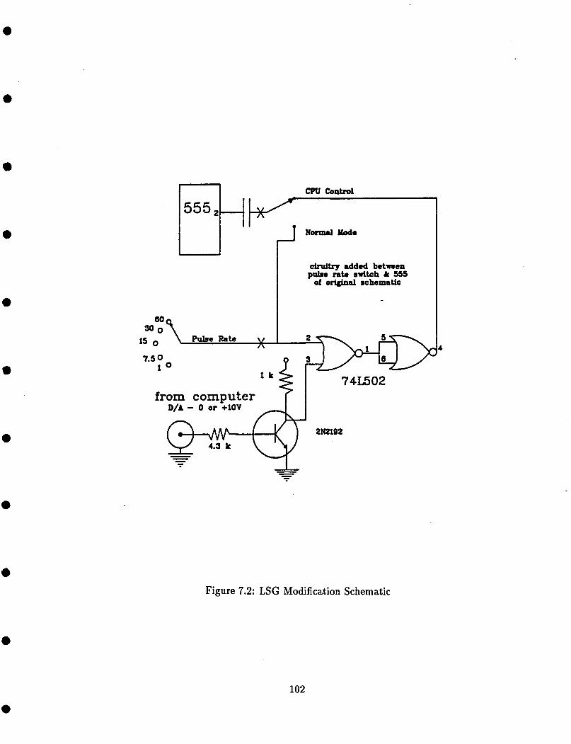
a

60

n CPU Control

c&ultry added between pulse rate switch & 555

of original schematic

4

Figure 7.2: LSG Modification Schematic

102

0

Section 8

a

APPENDIX C.l: PSP Set-up Program

C

C C+++++++++++++++++++++++++++++++++++++++++++++++++++++++++++++++- ++++++++++++ c C PROGRAM DEVELOPED TO SET-Up OPERATING PARAMETERS FOR THE C THE PARTICLE SIZING PROGRAM UTILIZING A MENU-TYPE FORMAT. C C+++++++++++++++++++++++++++++++++++++++++++++++++++++++++++++++- +++++++++++ c

BOUNDRY (2)

PROGRAM MENU

REAL*8 PROCESS(2), YESN0(2), ADVANCE(21, LIMIT(31,

INTEGER TOD(4) , DOY ( 5 ) CHARACTER*lO NUMBER

CHARACTER*l L(6), M(6) LOGICAL*l IKEY BYTE ESC, LINE(50,4) DATA ESC / 27 / DATA PROCESS, YESNO / 'STATIC', 'DYNAMC', 'YES ', 'NO

DATA LIMIT, FILE2 / 'TIME ', 'FRAME ', 'PARTCL', 'TEMPOI' /

REAL*8 MAG(2), A, B, C, D, F, G, H, I, J, V, W

CHARACTER*6 FILEl, FILE2

' / DATA ADVANCE, FILE1 / 'SINGLE', 'AUTO ', 'TEMPO1' /

DATA BOUNDRY, MAG / 'PROCSS', 'REJECT', 'LOW ', 'HIGH ' / DATA

DATA DATA DATA DATA DATA

2000 / IGPST, WIDTH, NGRPS, ITHRSH, LIMVAL / 5 , 5.0, 5 0 , 90, DATA JXSTR, JXDST, JYSTR, JYDST / 5 0 , 400, 50, 400 /

A, B, C, D / 'DYNAMC', 'YES ', 'AUTO ', 'PARTCL' / F, C, H, I / 'REJECT', 'YES ', 'YES ', 'YES ' / J , V, W / 'NO ', 'LOW ','NO ' / LINE / 200*' ' / NUMBER / '1234567890' /

EQUIVALENCE(L , FILE11 EQUIVALENCE(M , FILE21 CALL DATE(D0Y) CALL TIME(T0D) WRITE(7,l) ESC, ESC, ESC, ESC

103

e

1 FORnAT(lX,Al,’~8l’,A1,’~?251’,Al,’[H’,A1,’[2J’) C C*** IF DATE NOT SET, INSERT “NO DATE” INTO DATE FIELD C

IF( DOY(1) .EQ. ’00’ ) DOY(5) = ’ ’ IF( DOY(1) .EQ. ’00’ ) DOY(4) = ’TE’ IF( DOY(1) .EQ. ’00’ DOY(3) = ’DAB IF( DOY(1) .EQ. ’00’ DOY(2) = ’0 ’ IF( DOY(1) .Ed. ’00’ ) DOY(1) = ’ N’

C C C... C

INPUT PREVIOUSLY STORED PSP PARAMETERS.

OPEN(UNIT=l, FILE=’SETUP.MNU’ ,STATUS=’OLD’ ,ERR= 5) READ(1,lO) A,. B, C, D, LIMVAL, F, G, H, FILE1, I, J, FILE2,

& IGPST, WIDTH, NGRPS, JXSTR, JXDST, JYSTR, JYDST, ITHRSH, v, w READ(1,2) 2 FORMAT(2(/))

DO 4 II=1,4 READ(1,3) (LINE(JJ,II), JJ=1,50)

3 FORnAT(3X,50Al) 4 CONTINUE

WRITE(1,lO) A, B, C, D, LIMVAL, F, G, H, FILEl, I, J, FILE2, GOT0 9 5 OPEN(UNIT=l, FILE=’SEnrP.MNV’,STATUS=’NEW’)

& IGPST, WIDTH, NGRPS, JXSTR, JXDST, JYSTR, JYDST, ITHRSH, V, W WRITE(l,2) DO 6 II=1,4 WRITE(1,3) (LINE(JJ,II), JJ=l,SO)

WRITE(7,lO) A, B, C, D, LIMVAL, F, G, H, FILE1, I, J, 6 CONTINUE 9 FILE2, & IGPST, WIDTH, NGRPS, JXSTR, JXDST, JYSTR, JYDST, ITHRSH, V, W CLOSE(UN1T-1) 10 FORnAT(’+’,T39,’SETUP’/T26,’PARTICLE SIZING PROGRAM (ver. 4) ’// & 33(’-’) ,’ PROCESSING OPTIONS’ ,T54,25(’-’)/

& T3,’(A)’,T9,A6,T19,’Type of Processing’,T49, k ’(STATIC/DYNAMIC)’,/ & T3, ’ (B) ’ ,T9,A6,T19, ’FOCUS Criteria’ ,T49, & ’ (YES/NO) ’ , / & T3,’(C)’,T9,A6,Tl9,’Type of Frame Advance’,T49, & ’ (AUTO/SINGLE) ’ , / 8 T3,’(D)’,T9,A6,Tl9,’Processing Lirnit’,T49, & ’ (TIME/FRAME/PARTICLE) ’ , / & T3,’(E) (’,T9,16,T15,’) Limiting Value’,T49, & ’ (seconds/frames/particles)’ ,/ k T3,’(F)’,T9,A6,T19,’Boundary Particles’,T49, & ’(PROCESS/REJECT)’,/

104

a

~0 I l

a

a

0

a

a

a .

a

k 36(’-’) ,’ OUTPUT OPTIONS ’ ,26(’-’)/ b T3,’(C)’,T9,A6,Tlg,’General Results (to PRINTER)

k Tl9,’WRITE TO FILE (YES/NO)’,T49, k ’(K) FILE HEADER (4 lines)’,/ k T3,’(H)’,T9,A6,Tlg,’Average Particle size data -- ’,T49, b T3,’(I)’,T9,A6,T19,’Group Breakdown data ’ ,9( ’ - ’ ) , ’ / ’ /

(YES/NO) ’ /

k ’(L) FILE: (’,AS,’>.OUT’,/

& T3, ’ (J) ’ ,T9,A6,T19, ’Per Frame data ’ , 13(’-’), ’> ’ ,T49, & ’ (M) FILE : ( ’ , A6, ’ . DAT ’ , /

k 35(’-’) ,’ GENERAL OPTIONS ’,26(’-’)/ k T3,’(N) Group Start =( ’,13,’) ’ k T29,’(0) Group Width =(’,F4.1,’) ’ k T55,’(P) X of Groups =( ’,13,’)’/ k T3,’(q) X Window Start = (’#I3,’)’, b T49,’(R) X Window Width = (’,13,’)’/ k T3,’(S) Y Window Start = (’,13,’)’, & T49,’(T) Y Window Width = (’,13,’)’/ & T3,’(U) Threshold = (’,13,’)’ & T29, ’ (V) Lens = ’ ,A6, & T49, ’ (W) Markers = ’ , A6 , ’ (YEWNO) ’ /78 ( ’ - ’ WRITE(7,20) ESC, ESC FORMAT(’+’,Al,’[23;2H’,Als’[OJ’,’(X) to exit SETUP menu or 20

’/ “‘P & (Z) to begin Particle Sizing Program & T3,’Enter Letter to change specific Parameter ??’I

C C C ... C 30 CALL IPOKE(”44,”10000 .OR. IPEEK(”44))

SPECIFY PSP PARAMETER W/ KEY TOGGLE OR KEYBOARD ENTRY.

IKEY = ITTINRO IF(1KEY .LT.O) GOTO 30 IF(1KEY .EQ .’A’> GOTO 100 IF(IKEY.Eq.’B’) GOTO 200 IF(IKEY.EQ.’C’) GOTO 300 IF(IKEY.EQ.’D’) GOTO 400 IF(IKEY.Eq.’E’) GOTO 500 IF(IKEY.Eq.’F’) GOTO 600 IF(IKEY.Eq.’G’) GOTO 700 IF(IKEY.Eq.’H’) GOTO 800 IF(IKEY.Eq.’I’) GOTO 900 IF(IKEY.EQ.’J’) GOTO 1000 IF(IKEY.EQ.’K’) GOTO 1100 IF(IKEY.Eq.’L’) GOTO 1200 IF(IKEY.Eq.’M’) GOTO 1300 IF(1KEY .Eq. ’N’ GOTO 1400 IF(IKEY.Eq.’O’) GOTO 1500

105

a

C

90 0

C c... C 100

0

a

a

a

a

150 180 190

c... C 200

250 280 290

C C. .. C 300

350 380 390

IF(IKEY.EQ.’P’) GOTO 1600 IF(IKEY.EQ.’Q’) GOTO 1700 IF(1KEY .EQ. ’R’) GOTO 1800 IF(IKEY.EQ.’S’) GOTO 1900 IF(IKEY.Eq.’T’) GOTO 2000 IF(IKEY.Eq.’U’) GOTO 2100 IF(IKEY.Eq.’V’) GOTO 2200 IF(IKEY.EQ.’W’) GOTO 2400 IF(IKEY.Eq.’X’) GOTO 2600 IF(IKEY.Eq.’Y’) GOTO 2500 IF(1KEY. Eq . ’Z’ ) GOTO 2600 GO TO 30 FORMAT(’+’,A1,’[23;2H’,Al,’[OJ’,

k ’Enter new value for (’,Al,’) here ==>’,$I

(A) SPECIFY PROCESS TYPE (DYNAHIC/STATIC)

CALL IPOKE(”44,”167777 .AND. IPEEK(”44)) IF(A.EQ.PROCESS(1)) GOTO 150 A = PROCESS(1) GOTO 180 A = PROCESS(2) WRITE(7,190) ESC, A FORMAT ( ’ + ’ ,A1 , ’ [S ; 8H ’ , A6) GOTO 30 C (B) SPECIFY FOCUS (YES/NO)

CALL IPOKE(”44,”167777 .AND. IPEEK(”44)) IF (B . Eq . YESNO ( 1) ) GOTO 250 B = YESNO(1) GOTO 280 B = YESNO(2) WRITE(7,290) ESC, B FORMAT(’+’,Al,’[6;8H’,A6) GOTO 30

(C) TYPE OF FRAME ADVANCE (SINGLEJAUTO)

CALL IPOKE ( “44, It 167777 . AND. IF(C.EQ.ADVANCE(1)) GOTO 350 C = ADVANCE(1) GOTO 380 C = ADVANCE(2) WRITE(7,390) ESC, C FORMAT(’+’,A1,’[7;8H’,A6) GOTO 30

IPEEK ( “44) 1

106

0

a

~a

a

C c.. . C... 400

450

470 480 490

a

e

C C.. C 500

580 590

a

a

a

a

a

C c.. . C... C 600

650 680 690

C c... C 700

750 780 790

(D) PROCESSING LIMIT (TIME/PARTICLE/FRAME) NOTE: DUE TO COMPUTER LIMITATIONS TIME IS NOT INCLUDED C CALL IPOKE("44,"167777 .AND. IPEEK("44)) IF(D.EQ.LIMIT(1) .OR.D.EQ.LIMIT(2)) GOTO 450 D = LIMIT(1) GOTO 480 IF(D.EQ .LIMIT(2) 1 GOTO 470 D = LIMIT(2) GOTO 480 D = LIMIT(3) WRITE(7,490) ESC, D FORMAT('+',Al,'C8;8H',A6) GOTO 30

(E) SPECIFY LIMITING VALUE

CALL IPOKE("44,"167777 .AND. IPEEK("44)) WRITE(7,90) ESC, ESC, 'E' READ(5,*) LIMVAL WRITE(7,590) ESC, LIMVAL FORMAT('+' ,Al,' [9;8HJ ,161 WRITE(7,20) ESC, ESC GOTO 30

(F) BOUNDARY ANALYSIS NOTE: UNAVAILABLE

CALL IPOKE("44,"167777 .AND. IPEEK("44)) IF(F.EQ.BOUNDRY(1)) GOTO 650 F = BOUNDRY(1) GOTO 680 F = BOUNDRY(2) WRITE(7,690) ESC, F FORMAT('+',Al,' [10;8H' ,A61 GOTO 30

(G) OUTPUT GENERAL RESULTS TO PRINTER

CALL IPOKE ("44, I' 167777 . AND. IPEEK ( "44) ) IF(G.EQ.YESNO(1)) GOTO 750 G = YESNO(1) GOTO 780 G = YESNO(2) WRITE(7,790) ESC, G FORMAT('+' ,Al, ' [12;8H' ,A6)

107

a

a

0

a

a

0

0

0

a

GOTO 30 C C... (HI WRITE TO FILE: ANALYSIS SUMMARY (YEWNO) C 800 CALL IPOKE(”44,”167777 .AND. IPEEK(”44))

IF(H.EQ.YESNO(1)) GOTO 850 H = YESNO(1) GOTO 880

850 H = YESNO(2) 880 WRITE (7,890) ESC , H 890

C C... (I) WRITE TO FILE: GROUP BREAKDOWN (YEWNO) C 900 CALL IPOKE(”44, “167777 .AND. IPEEK(”44) )

FORMAT(’+’ ,Al, ’ [14;8H’ ,A6) GOTO 30

IF(1 .EQ .YESNO (1) I = YESNO(1) GOTO 980

950 I = YESNO(2) 980 WRITE(7,990) ESC, I 990 FORMAT(’+’,Al,’[l5;8H’,A6)

C C.. . (J) WRITE TO FILE: PER FRAME DATA (YES/NO) C 1000 CALL IPOKE(”44, “167777 .AND. IPEEK(”44))

GOTO 950

GOTO 30

IF (J . EQ . YESNO ( 1) 1 GOTO 1050 J = YESNO(1) GOTO 1080

1050 J = YESNO(2) 1080 WRITE(7,1090) ESC, J 1090 FORMAT(’+’ ,Al,’ [16;8H’ ,A6)

C C... (K) SPECIFY FILE HEADER C 1100 CALL IPOKE(”44,”167777 .AND. IPEEK(”44))

1110

1111

GOTO 30

WRITE(7,lllO) ESC, ESC, ESC, ESC FORMAT(1X ,Ai, ’ C8l’ ,Ai, ’ [?251’ ,A1 , ’ [H’ ,Ai, ’ C2J’ ) WRITE(7,llll) ((LINE(JJ,II), JJ=l,SO), II=1,4) FORMAT(’+’ ,T39, ’SETUP’/T35, ’FOR FILE HEADER’//

k T36,’CHANGE (Y/N)’///T16,54(’*’),/T16,’*’,T69,’*’, k 4(/,T16,’* ’50A1,’ *’),/T16,’*’,T69,’*’, k /T16,54(’*’)//T31, ’(4 LINES/SO SPACES each) ’1 CALL IPOKE (“44, I’ 10000 . OR. IPEEK (“44) )

108

0

‘0

a

a

a

a

a

a

a

a

1115

1120

1125

IKEY = ITTINRO IF(IKEY.LT.0) GOTO 1115 IF(IKEY.EQ.’Y’) GOTO 1120 IF(IKEY.EQ.’N’) GOTO 1190 GOTO 1115 CALL IPOKE(tt44,”167777 .AND. IPEEK(”44)) DO 1140 II=1,4 WRITE(7,1125) ESC, ESC, I1 FORMAT( ’ + ’ ,Ai, ’ [I7 ; 3H’ , A1 , ’ [O J’ ,

k ’Change Line (’,Il,’), (Y/N)’) CALL IPOKE(tt44,”10000 .OR. IPEEK(”44))

IF(1KEY .LT.O) GOTO 1126 IF(IKEY.EQ.’Y’) GOTO 1127 IF(IKEY.EQ.’N’) GOTO 1140 GOTO 1126

WRITE(7,1130) ESC, ESC, ESC, I1

1126 IKEY = ITTINRO

1127 CALL IPOKE ( “44, I’ 167777 . AND. IPEEK ( “44) ) 1130 FORMAT(’+’,Al,’[22;lH’,Al,’[OJ’,Al,’[?8h’,

& ’ Line (‘,11,’) =I>’,$) IF(I1 .EQ. 1) GOTO 1141 IF(II.EQ.2) GOTO 1143 IF(II.EQ.3) GOTO 1145 IF(II.EQ.4) GOTO 1147

1140 CONTINUE GOTO 1180

1141 READ(5,1170) (LINE(JJ,l), JJ=l,SO) WRITE(7,1142) ESC, (LINE(JJ,l), JJ=l,SO)

1142 FORMAT(’+’,Al,’[9;lSH’,’* ’,50Al,’ *’) GOTO 1140

1143 FtEAD(5,1170) (LINE(JJ,2), JJ=l,SO) WRITE(7.1144) ESC, (LINE(JJ,2), JJ=l,SO)

1144 FORMAT(’+’,Al,’[lO;lSH’,’* ’,50A1,’ *’) GOTO 1140

1145 READ(5,1170) (LINE(JJ,3), JJ=l,SO) WRITE(7,1146) ESC, (LINE(JJ,3), JJ=l,SO)

1146 FORMAT(’+’,Al,’[ll;lSH’,’* ’,50Al,’ *’) GOTO 1140

1147 READ(5,1170) (LINE(JJ,4), JJ=l,SO) WRITE(7,1148) ESC, (LINE(JJ,4), JJ=l,SO)

1148 FORHAT(’+’,Al,’Cl2;15H’,’* ’,50Al,’ *’) GOTO 1140

1170 FORMAT(5OAl) 1180 GOTO 1100 1190 WRITE(7,l) ESC, ESC, ESC, ESC

GOTO 9

109

C c... C 1200

1220

(L) FILE SPECIFICATION: GENERAL & GROUP DATA

CALL IPOKE(”44,“167777 .AND. IPEEK(”44)) WRITE(7,1220) ESC, ESC, ’L’ FORMAT(’+’,Al,’[23;2H’,Al,’[OJ’,

& ’File Name (’,Al,’) (4 letters) here ==>’,$I READ(5,1230) (L(II), II=l,4)

WRITE(7,1240) ESC, (L(II), II=l,4)

WRITE(7,1250) ESC, ESC, ’L’ FORMAT(’+’ ,Al, ’ C23;2H’ ,Al,’ COJ’ ,

READ(5,1260> Ll 1260 FORMAT(I2)

I1 = Ll/lO IO = Ll-Il*lO IF(L1.LT. 10) 11-10 IF(I0 .EO. 0) IO=lO L(5) = NUMBER(I1:Il) L(6) = NUMBER(I0:IO) IF(Ll.LT.10) GOTO 1280 WRITE(7,1270) ESC, Ll

1270 FORMAT(’+’,Al,’C14;64H’,I2) WRITE(7,20) ESC, ESC GOTO 30

1280 WRITE(7,1290) ESC, Ll 1290 FORMAT(’+’ ,Al, ’ [14;64HO’ ,Il)

WRITE(7,20) ESC, ESC GOTO 30

1230 FORMAT(4Al)

1240 FORMAT(’+’,Al,’C14;60H’,4Al)

1250 k ’File Number (’ ,Al, ’1 (2 numbers) here ==>’ ,$)

C C... ( M I FILE SPECIFICATION: PER FRAME DATA C 1300 CALL IPOKE(”44, I’ 167777 . AND. IPEEK( “44) )

1320 WRITE(7,1320) ESC, ESC, ’M’ FORMAT(’+’ ,Ai, ’ C23;2H’ ,Ai, ’ [OJ’ ,

READ(5,1330) (M(II), II=l,4)

WRITE(7,1340) ESC, (M(II), II=1,4)

WRITE(7,1350) ESC, ESC, ’ M ’ FORMAT( ’+’ ,Ai, ’ c23 ; 2H’ ,Ai, ’ [OJ ’ ,

READ(5,1360) M1

& ’File Name (’,Al,’) (4 letters) here ==>’,$)

1330 FORMAT(4Al)

1340 FORMAT(’+’,Al,’C16;60H’,4Al)

1350 & ’File Number (’,Al,’) (2 numbers) here ==>’,$)

110

1360

1370

e

e

a

e

1380 1390

C C... C 1400

1480 1490

C c... C 1500

1580 1590

C C... C 1600

1680 1690

FORHAT(I2) I1 = Hl/lO IO Hi-Il*lO IF(H1 .LT. 10) 1140 IF(I0 .Eq. 0) IO=lO H ( 5 ) = "BER(I1: 11) H(6) = NUHBER(1O:IO) IF(H1 .LT. 10) GOTO 1380 WRITE(7,1370) ESC, H1 FORHAT('+' ,Al,' C16;64H' ,121 WRITE(7,20) ESC, ESC GOTO 30 WRITE(7,1390) ESC, Hl FORHAT( ' + ' ,A1 , ' c16 ; 64H0 ' ,111 WRITE(7,20) ESC, ESC GOTO 30

(N) DROP-SIZE GROUP BREAKDOWN: STARTING VALUE

CALL IPOKE("44,"167777 .AND. IPEEK("44)) WRITE(7,90) ESC, ESC, 'N' READ(5, *) IGPST WRITE(7,1490) ESC, IGPST FORHAT('+',Al,'C18;2lH',I3) WRITE(7,20) ESC, ESC GOTO 30

(0) DROP-SIZE GROUP BREAKDOWN: INTERVAL WIDTH

CALL IPOKE("44,"167777 .AND. IPEEK("44)) WRITE(7,90) ESC, ESC, ' 0 ' READ(S,*) WIDTH WRITE(7,1590) ESC, WIDTH FORHAT('+' ,Al, ' C18;46H' ,F4.1) WRITE(7,20) ESC, ESC GOTO 30

(PI DROP-SIZE GROUP BREAKDOWN: # OF GROUPS

CALL IPOKE ("44, It 167777 . AND. IPEEK ( "44) ) WRITE(7,90) ESC, ESC, 'P' READ(S,*) NGRPS WRITE(7,1690) ESC, NGRPS FORHAT('+',Al,' C18;73H8,13) WRITE(7,20) ESC, ESC GOTO 30

111

C C... C 1700

e

l

e 1780 1790 a

*

0

C c... C 1800

1880 1890

C c... C 1900

1980 1990

C c... C 2000

2080 2090

C c... C 2100

0

(Q) SIZING WINDOW (PIXEL SPEC): X STARTING VALUE

CALL IPOKE(t144,"167777 .AND. IPEEK("44) WRITE(7,90) ESC, ESC, 'q ' READ ( 5 , *) JXSTR WRITE(7,1790) ESC, JXSTR FORMAT('+' ,Al,' [19;24H' ,131 WRITE(7,20) ESC, ESC GOTO 30

(R) SIZING WINDOW (PIXEL SPEC): X SCREEN WIDTH

CALL IPOKE("44,"167777 .AND. IPEEK("44)) WRITE(7,90) ESC, ESC, 'R' READ(5, *) JXDST WRITE(7,1890) ESC, JXDST FORMAT('+',Al,' [19;72H',I3) WRITE(7,20) ESC, ESC GOTO 30

(S) SIZING WINDOW (PIXEL SPEC): Y STARTING VALUE

CALL IPOKE("44,"167777 .AND. IPEEK("44)) WRITE(7,90) ESC, ESC, 'S' READ(5,*) JYSTR WRITE(7,1990) ESC, JYSTR FORMAT('+',Al,'[20;26H',I3) WRITE(7,20) ESC, ESC GOTO 30

(T) SIZING WINDOW (PIXEL SPEC): Y SCREEN WIDTH

CALL IPOKE("44,"167777 .AND. IPEEK("44)) WRITE(7,90) ESC, ESC, 'T' READ ( 5 , *) JYDST WRITE(7,2090) ESC, JYDST FORMAT('+',Al,'[20;7OH',I3) WRITE(7,20) ESC, ESC GOTO 30

(U) INPUT SIZING THRESHOLD

CALL IPOKE("44,"167777 .AND. IPEEK("44) ) WRITE(7,90) ESC, ESC, 'U' READ(5,*) ITHRSH

112

a

2180 I 2190 ~0 I

I

C c... C 2200 a

a

a

a

0

2250 2280 2290

C C... C 2300

2350 2380 2390

C c.. . C 2600

WRITE(7,2190) ESC, ITHRSH FORMAT('+' ,Al,' [21;19H' ,131 WRITE(7.20) ESC, ESC GOTO 30

(V) INPUT SYSTEM MAGNIFICATION (HIGH/LOW)

CALL IPOKE("44,"167777 .AND. IPEEK("44)) IF(V.EQ.MAG(1)) GOTO 2250 V = MAG(1) GOTO 2280 V = MAG(2) URITE(7,2290) ESC, V FORMAT('+' ,Al,' [21;39H',A6) GOTO 30

(W) DIAGNOSTIC MARKERS

CALL IPOKE ( "44, I) 167777 IF(W.EQ.YESNO(1)) GOTO W = YESNO(1) GOTO 2380 W = YESNO(2) WRITE(7,2390) ESC, W

PLACED ON COUNTED PARTICLES

. AND. IPEEK ("44) 2350

FORMAT('+',A1,'[21;62H',A6) GOTO 30

(2) STORE SET-UP PARAMETERS AND START PSP

CALL IPOKE("44,"167777 .AND. IPEEK("44)) OPEN(UN1T-I, FILE='SEnrP.MNv',STAnrSt'N~') WRITE(1,lO) A, B, C, D, LIMVAL, F, G, H, FILE1, I, J,

FILE2, & IGPST, WIDTH, NGRPS, JXSTR, JXDST, JYSTR, JYDST, ITHRSH, V, W WRITE ( 1,2605) 2605 FORMAT(2(/))

DO 2650 II=I,4 WRITE(1,2610) (LINE(JJ,II), JJ=1,50)

2610 FORMAT(3X,SOAl) 2650 CONTINUE

CLOSE(UNIT=l) WRITE(7,2690) ESC, ESC, ESC, ESC

IF(IKEY.EQ.'Z') CALL SETCMD('RUN PSPI') CALL EXIT

END

2690 FORMAT(lX,AI,'[8h',A1,'~?25h',AI,'[H',AI,'C2J'~

2700 STOP

113

*

e

a

e

a

e

a

Section 9

APPENDIX C.2: PSP Graphical Presentation of Results

C

. . . . . . . . . . . . . . . . . . . . . . . . . . . . . . . . . . . . . . . . . . . . . . . . . . . . . . . . . . . . . . . . +++++++++++ c C

. . . . . . . . . . . . . . . . . . . . . . . . . . . . . . . . . . . . . . . . . . . . . . . . . . . . . . . . . . . . . . . . . +++++++++++ c

PROGRAM GRAPH

PROGRAM DEVELOPED FOR THE PSP TO GRAPHICALLY REPRESENT C THE GROUP BREAK-DOWN DATA ON A DEC COMPATIBLE TERMINAL. C

DIMENSION X(lOOO), Y(lOOO), Yl(70) , Xl(70) BYTE ESC, CSI, TIM(91, DAY(9) CHARACTER*l A, B, C, H, 11, NUMXO, NUMYO, NUMXl, NUMY1

CHARACTER*l NAME(7) , JUNK CHARACTER*lO NUMBER, FILE DATA A, ESC, CSI /'*', 27, 155 / DATA B, C, H /'[', ';', 'f'/ DATA NUMBER / '1234567890' / DATA CO, PI / ' ', 3.1415926 / EQUIVALENCE (NAME(1) ,B) EQUIVALENCE (NAME(2),"Xl) EQUIVALENCE (NAHE(3),NUMXO) EQUIVALENCE (NAME(4) ,C) EQUIVALENCE (NAME(5) ,"MYl) EQUIVALENCE (NAME(6) ,NUMYO) EQUIVALENCE (NAME(7),H)

X(I)=O.O Y (I)=O. 0

5 CONTINUE

CHARACTER* 11 CO

1 DO 5 I=1,1000

DAVSUM = 0.0 DSSUM = 0.0 DVSUH = 0.0 DWSUM = 0.0 SUMN = 0.0 SUM = 0.0

114

6 C C... C

10

20

30 40

50

60

70

80 90 C C.. C

.WEIGHT = 0.0 COUNT = 0.0 DO 6 I=1,70 x1 (I) =O .o Y 1 (I) 10.0 CONTINUE

INPUT DATA FILE NAME.

WRITE(7,lO) FORMAT(lX, ’ INPUT DATA FILE ==> ’ ,$) READ(5,20,ERR=200)FILE FORMAT (A10 ) OPEN(UNIT=2,NAME=FILE,STATUS=’OLD’) DO 30 I=1,1000 READ(2,*,END=40) X(1) ,Y(I) CONTINUE INDEX = 1-1 IF(INDEX.EQ.68) GO TO 94 YMAX = -1.OE+30 XMIN = l.OE+30 XMAX = -1.OE+30 DO 50 K=l,INDEX XMIN = AMINl (XMIN ,Y (K) ) XMAX = AMAXl(XMAX,Y(K)) XCEN = (XMIN+XMAX)/2.0 XSCALE (XMAX-XMIN)/67.0 DO 60 J=1,67 Xi (J) =XMIN+XSCALE*FLOAT(J) CONTINUE DO 90 L=l,INDEX DO 70 M=1,67 IF(Y(L).GT.Xl(M)) GO TO 70 GO TO 80 CONTINUE M-68 Yl(M)=Yl(M)+l.O CONTINUE

STATISTICAL MEAN DIAMETERS DETERMINED

DO 93 I=1,67 IF(I.EQ.1) GRPAVG = Xl(I)/2.0 IF(I.NE.1) GRPAVG (Xl(I)+Xl(I-1))/2.0 DIAMAX = YMAX DAVSUM = DAVSUM + Yl(I)*GRPAVG

115

e

e

93

e

e 94

0 95

0

e

e

e

e

97

100

C c.. a

c... C

105

DSSUM = DSSUM + DVSUM’ = DVSUM + DWSUM = DWSUH + SUHN =SUMN + SUM =SUM + WEIGHT = WEIGHT + CONTINUE DAV = DAVSUM/SUMN DS = SQRT(DSSUM/SUM) DV = (DVSUM/SUMN) ** (1. /3. ) DVS = DVSUM/DSSUM DW = DWSUM/DVSUM NSUM = IFIX(SUM) GOTO 97 REWIND (2) READ (2, *) GCD , DAV ,DS , DV ,DVS ,DW DO 95 K=1,67 Xl(K) = X(K+l) Yl(K) = Y(K+l) CONTINUE XMAX = Xl(67) XMIN = Xi (1) - (Xl(67) -X1(66) ) XCEN = (XMIN+XMAX) /2.0 XQUA = (XCEN-XMIN)/2.0 X14 = XMIN + XQUA X34 = XCEN + XQUA COUNT=O . 0 DO 100 K=1,67 COUNT=COUNT + Yl(K) YMAX = AMAXl(YMAX,Yl(K)) CONTINUE NSUM = IFIX(C0UNT) YSCALE = YMAX/21.0 YSCALl = YMAX/l99.0 IYMAX = IFIX(YMAX) IYCEN = IFIX(.SO*YMAX) IY14 = IYCEN/2 IY34 = IYCEN + IY14

UTILIZING THE PSEUDO-GRAPHIC CAPABILITIES OF DEC COMPATIBLE TERMINALS: INITIATE GRID.

CALL CHARGR WRITE (7,105) ESC , ESC FORMAT(’+’,Al,’*O’,Al,’n’) WRITE(7,llO) ESC, ESC, ESC, ESC

116

e

e

e

e

e

e

e

e

e

e

110 FORMAT(lX,Al,’[H’,A1,’[2J’,Al,’[?3h’,A1,’[?251’) WRITE(7,llS) CO(1:l) ,IYMAX

e 115 FORMAT(’+’ ,lX,A1,2X,I4,2X,’w’ ,16(’q’) ,’w’ ,16(’q’) ,’w’ , k 16(’qJ),’w’,16(’q’),’k’)

117 FORMAT(2X,Al,2X,14,2X,’n’,16(8q’) ”nS,l6(’q’) ,’n’ , % 16( ’q’ 1, ’n’ ,16(’q’), ’u’) 120 FORMAT(2X,A1,8X,’nB ,16(’q3) ,’n3 ,16(’q’) ,’n’,

DO 130 M=1,19 Mi44 IF(M.EQ. 5)WRITE(7,117) CO(Ml:Ml), IY34 IF(M.EQ. 5) GOTO 130 IF(M.GT. 5) GOTO 122 GOTO 128

IF(M.Eq. 10) GOTO 130 IF(M.GT.10) GOTO 124 GOTO 128

IF(M.EQ.l5>WRITE(7,117) CO(Ml:Ml), IY14 IF(M.Eq. 15) GOTO 130

k 16( ’q’), ’n’ ,16(’q’), ’u’)

122 IF(M.EQ. lO)WRITE(7,117) CO(Ml:Ml), IYCEN

124 Ml=l

128 WRITE(7,140) CO(M1:Ml) 130 CONTINUE 140 FORMAT(~X,AI,~X,’X’,~~X,’~’,~~X,’X’,

% 16X,’x’,16X,’x’) WRITE(7,120) GO ( 1 : 1) WRITE(7,145) ESC, ESC, ESC

145 FORMAT(’+’,Al,’*B’,Al,’n’,Al,’[Om’) WRITE(7,146) XMIN, X14, XCEN, X34, XMAX

146 F0RMAT(8X,F5.1,12X,F5.1,12X,F5.1,12X,F5.1,12X,F5.1, %’ //37X, ’DIAMETER [microns] ’ )

WRITE(7,161) ESC, ESC WRITE(7,147) E X , ESC, ESC, ESC, ESC, ESC

147 FORMAT(’+’,Al,’[7;2f 5’, % A1,’[8;2f 6’, % A1,’[9;2f 7’, % A1,’[10;2f 8’, % A1,’[11;2f 9’, & A1,’[12;2f :’)

161 FORMAT(’+’,Al,’* O’,Al,’n’) DO 168 J = 12,78 Jl = J/lO JO J - Jl*lO IF(J.LT. 10) Jl=lO IF(JO.EQ.O)JO=lO NUMYO = NUMBER(J0: JO)

117

a

a

e

a

0

a

C c.. . C

162 163 164 165 166

167 250

" Y 1 = NUMBER(J1:Jl)

HISTOGRAn SCREEN PLOT

52 = J-11 IF(Yl(J2) .LE.O.O) GOTO 168 IN2 = 4 NNl = IFIX(Yl(J2)/YSCALl) I1 = 2 IO = 1 NUMXO = NUMBEN10 : IO) NUMX1 = NUMBER(I1:Il) IF(NNl.GT.4) GOTO 162 IF(NNl.EQ.1) WRITE(7,163) ESC, (NAME(K) ,K=1,7) IF(NNI.EQ.2) WRITE(7,164) ESC, (NAME(K) ,K=1,7) IF(NNl.EQ.3) WRITE(7,165) ESC, (NAME(K) ,K=1,7) GOTO 168 WRITE(7,166) ESC, (NAME(K) ,K=l,7) FORMAT('+',Al,7Al,'l') FORMAT( ' +' , A1 ,7Al, '2' FORMAT('+' ,A1,7Al, '3') FORMAT( ' +' , A1 ,7Al, '4' ) DO 167 I = 20,1,-1 NN2 = NN2 + 10 IF(NN2.GT.NNl) GOTO 250 I1 = 1/10 IO = I - Il*lO IF(I.LT.lO)Il=lO IF(IO.EQ .O)IO=lO NUMXO = NUMBER(I0:IO) NUMXl = NUMBER(I1:Il) WRITE(7,169) ESC, (NAME(K) ,K=1,7) CONTINUE NN2 NN2 - 10 NN2 = NNl - NN2 I1 = 1/10 IO = I - Il*lO IF(1. LT. 10) Il=lO IF(I0 .EQ .O ) I0=10 NUMXO = "MBER(I0:IO) NUMX1 = "MBER(I1:Il) IF(NN2.EQ. 1) WRITE(7,301) ESC, (NAME(K) ,K=1,7) IF(NN2.EQ.2) WRITE(7,302) ESC, (NAME(K),K=1,7) IF(NN2.EQ.3) WRITE(7,303) ESC, (NAME(K),K=1,7) IF(NN2.EQ.4) WRITE(7,304) ESC, (NAME(K),K=1,7) IF(NN2.EQ.5) WRITE(7,305) ESC, (NAME(K),K=l,7)

118

e

a

a

a

a

0

a

IF(NN2. EQ .6) WRITE(7,306) ESC , (NAHE(K) ,K=l ,7) IF(NN2.EQ.7) WRITE(7,307) ESC, (NAHE(K) ,K=l,7) IF(NN2 .EQ. 8) WRITE(7,308) ESC, (NAME(K) ,K=1,7) IF(NN2.EQ.9) WRITE(7,309) ESC, (NAME(K1 ,K=1,7)

168 CONTINUE 30 1 FORMAT(’+’,Al,fAl,’A’) 302 FORMAT(’+’,Al,7Al,’B’) 303 FORMAT(’+’ ,A1,7A1, ’C’) 304 FORMAT(’+’ ,A1,7Al,’D’) 305 FORMAT(’+’ ,A1,7Ai,’E’)

307 FORMAT(’+’ ,A1,7Al, ’G’) 308 FORMAT(’+’ ,AI ,7Al, ’€I3 ) 309 FORMAT( ’ +’ , A1 , 7Al , ’ I ) 169 FORMAT( ’+’ ,AlJ7A1, ’ J’) C C... OUTPUT MEAN DIAMETERS TO SCREEN C

306 FORMAT(’+’,Al,7Al,’F’)

WRITE(7,145) ESC, ESC, ESC CALL DATE(DAY) CALL TIME(T1M) WRITE(7,170) ESC

170 FORMAT(’+’ ,AI, ’ [3;85f’, ’Spatial Distribution . . . . . . . . . ’1 WRITE(7,171) ESC, GCD 17 1 FORMAT(’+’,AlJ’[5;85f’ ,’ Most Probable Dia. =’,F7.1) WRITE(7,172) ESC, DAV 172 FORMAT(’+’,Al,’C6;85f’,’ Arithmetic Mean Dia. (DIO) =’ ,F7.1) WRITE(7,173) ESC, DS 173 FORMAT(’+’,A1,’[7;85f’,’ Surface Mean Dia. (D20) =’,F7.1) WRITE(7,174) ESC, DV 174 FORMAT(’+’,AlJ’C8;85f’,’ Volume (Mass) Mean Dia. (D30) =’ ,F7. I) WRITE(7.175) ESC, DVS 175 FORMAT(’+’,AI,’[9;85f’,J Sauter Mean Dia. (D32) =,,F7.1) WRITE(7,176) ESC, NSUM 176 =’ ,171 177

178

179

198

199

FORMAT(’+’,AlJ’[1l;85f’,’ Total Count

FORMAT(’+’,Al,’[16;85f’,’ File: ’,AI01 WRITE(7,178) ESC, DAY FORMAT(’+’,Al,’[17;85fJ ,’ Date: ’,9Al) WRITE(7,179) ESC, TIM FORMAT(’+’,A1,’[18;85fJJ~ Time: ’,9A1) READ(7,198) JUNK FORMAT (A 1) WRITE(7,199) ESC, ESC, ESC, ESC, ESC FORMAT(lX,Al,’ [Om’,AI,’[H’,Al, J[?31’,AI,’[2JJ,Al,’[?25h’) CLOSE (2)

URITE(7 , 177) ESC, FILE

119

a

a

e 200

CALL SETCMD(’RUN GRAPH’) CALL EXIT STOP END

m

e

,a

0

e

0

a

C c... C

147

148

149

150

15 1

152

153

154

155

156

157

158

159

160

161

162

163

164

SUBROUTINE UTILIZED TO SET-UP HISTOGRAM SYMBOLS

SUBROUTINE CHARGR BYTE ESC DATA ESC / 27 / WRITE(7,147) ESC , ESC FORMAT(’+’ ,Al,’P0;33;1;0;0;0( O???????/GGGGGGG’,Al,’\’)

FORMAT( ’ +’ ,Ai, ’PO; 34; 1 ; 0; 0; O( O???????/KKKKKKK ’ , A1 , ’ \ ’ )

FORMAT( ’ +’ , Ai, ’PO ; 35 ; 1 ; 0; 0 ; O( O???????/MMMMMMM ’ ,Ai, ’ \ ’ )

FORMAT( ’ +’ ,Ai, ’PO ; 36 ; 1 ; 0; 0 ; O( O???????/NNNNNNN’ ,Ai, ’ \ ’ )

FORMAT(’+’ ,Al,’P0;37;1;0;0;0( 0 _ _ _ _ _ _ _ _ /NNNNNNN’ ,Al,’\’) WRITE(7,lSZ) ESC, ESC FORMAT(’+’,Al,’PO;38;1;0;0;0~ Oooooooo/NNNNNNN’,Al,’\’)

FORMAT(’+’,Al,’P0;39;1;0;0;0( Ouuuuuuu/NNNNNNN’ ,Al, ’\’I

FORMAT( ’ +’ ,Ai, ’PO ; 40; 1 ; 0; 0 ; O( OC((((((/NNNNNNN’ ,Ai, ’ \ ’ )

FORMAT(’+’,Al,’PO;41;1;0;0;0~ O)))))))/NNNNNNN’ ,Al,’\’)

FORMAT(’+’,Al,’PO;42;1;0;0;0( O-’-””- /NNNNNNN’,Al,’\’)

FORMAT(’+’,Al,’PO;17;1;0;0;0~ OWWWWWWW/???????’,Al,’\’)

FORMAT(’+’,AI,’P0;18;1;0;0;0< OCCCCCCC/???????’ ,Al,’\’)

FORMAT(’+’ ,Al,’PO;l9;l;O;O;O~ Ollll1ll/???????’,Al,’\’)

FORMAT(’+’,A1,’P0;20;1;0;0;0( O^^^^^^^ /???????’,Al,’\’)

FORMAT(’+’,Al,’PO;21;1;0;0;0~ ONOOMOOI/???????’ ,Al,’\’)

FORMAT( ’ +’ ,Ai, ’PO; 22 ; 1 ; 0; 0; O c O^CCCCCC/??????? ’ ,Ai, \ )

FORMAT(’+’,Al,’P0;23;1;0;0;0< OPXTTTRP/???????’,Al,’\’)

FORMAT(’+’ ,Al,’PO;24;1;0;0;0( OPPPPPPM/???????’ ,Al,’\’)

WRITE(7,148) ESC, ESC




WRITE(7,153> ESC, ESC


WRITE(7,lSS) ESC, ESC

WRITE(7,lSS) ESC , ESC

WRITE(7,157) ESC , ESC

WRITE(7,158> ESC , ESC






WRITE(7,164) ESC , ESC

120

e

e

‘a

e

e

WRITE(7,165) ESC, ESC 165 FORHAT(’+’,Al,’P0;2S;l;O;O;O~ OHPPPPPH/???????’,Al, ’\’I

WRITE(7,166) ESC, ESC 166 FORHAT( ’+’ ,A1 , ’PO; 26 ; 1 ;O; 0; OC OHPOOOPH/???????’ ,Ai, ’\’ )

CALL EXIT STOP END

121

e

Section 10

e

e

a

0

e

e

APPENDIX C.3: MOD-1 Nozzle Input Pressure Determination

C

C++++++++++++++++++++++++++++++++++++++++++++++++++++++++++++++++- +++++++++++ c C SUBROUTINE TO DETERMINE WATER AND AIR PRESSURE FROM C

C+++++++++++++++++++++++++++++++++++++++++++++++++++++++++++++++- +++++++++++ LOGICAL*l IKEY

SUBROUTINE PRESSURE(NCHCK)

THE OMEGA TRANSDUCERS USING THE AXVl1-C A-D BOARD. C

BYTE ESC DATA ESC / 27 / CALL IPOKE("44 , "10000. OR. IPEEK("44))

C c... c... c... C

C

10

11 C C... C 12 13

C c... C... C

THE FOLLOWING ARE THE APPROPRIATE OCTAL VALUES TO

A TO D CONVERSION OF THE PRESSURE TRANSDUCERS. BE STORED IN THE CSRs OF CH. 1 k 2 TO START AN

ISTRTl = "415 ISTRT2 = "1015

IF(NCHCK .EQ .1) GOTO 12 WRITE(7 , 10) ESC , ESC , ESC FORMAT( '+' ,A1 , ' [ZJ' ,Ai, ' [?251' ,Al, ' [H') WRITE(7 , 11) ESC FORMAT(lX,Al,'#6',' PRESS tlC1l to continue')

17770400 IS THE CSR (CONTROL STATUS REGISTER) FOR CH. 1

CALL IPOKE("17770400 , ISTRTl) ICHK = IPEEK("l7770400) IF(ICHK.NE."614) GOTO 13

17770402 IS THE DBR (DATA BUFFER REGISTER) FOR CH. 1 AND IPW IS THE WATER PRESSURE (DIGITAL VOLTS).

IPW = IPEEK("l77770402)

122

0

e

8

r)

CALL IPOKE(”17770400, ISTRT2) ICHK = IPEEK ( I’ 17770400) IF(ICHK.NE.”l214) GOTO 14 IPA = IPEEK ( I’ 17770402) IPA = -1.189 + 0.4598*IPA IPW -1.95 + 0.4598*IPW

14

C C... OUTPUT PRESSllRE VALUES TO TERMINAL SCREEN C

WRITE(7,18) ESC, ESC, IPU, IPA WRITE(7,lS) ESC, ESC, IPW, IPA IF(NCHCK.Eq. 1) GOTO 25

IF(IKEY.EQ.’C’) GOTO 20 GOTO 12

IKEY = ITTINR~

18 FORMAT(’+’,Al,’[22;lf’,A1,’#3’,’WATER PRESSURE = ’, & 13,’ AIR PRESSURE = ’,I31 19

20

21 25

& 13,’ FORMAT(’+’,Al,’[23;lf’,A1,’#4’,’#WATER PRESSURE = ’, AIR PRESSURE = ’ ,131 CALL IPOKE( “44, “167777. AND. IPEEK (“44) WRITE (7,211 ESC , ESC FORMAT(’+’,Al,’[H’,Al,’[2J’) RETURN END

123

e

e

Section 11

APPENDIX C.4: PSP Magnification Correction Factor Determination

e

e

e

e

a

e

e

C ................................................................. ++++++++ c C FUNCTIONS TO DETERMINE CORRECTION FACTORS FOR C MICRON TO PIXEL FACTORS WHICH DEPEND ON X AND Y. C C+++++++++++++++++++++++++++++++++++++++++++++++++++++++++++++++- ++++++++ FUNCTION XFACT(MAG,XPOS,YPOS)

C C... HIGH MAGNIFICATION X-CORRECTION C

IF (MAG. EQ . 500) GOT0 100

IF(XP0S. LE. 100.0) XFACT=O .977+YPOS*8.09E-05 IF(XPOS.GT.lOO.O.AND.XPOS.LE.15O.O)

XFACT=0.974+YPOS*2.6OE-05 IF(XP0S. GT. 150.0. AND. XPOS .LE. 200.0) XFACT=O .967-YPOS*8.12E-07

IF(XPOS.GT.200 .O.AND.XPOS.LE.250.0) XFACT=O .961+YPOS*4.73E-06 IF(XPOS.GT.250.0.AND.XPOS.LE.300.0) XFACT=0.961-

YPOS*5.46E-05 IF(XPOS.GT.300.0.AND.XPOS.LE.350.0) XFACT=O. 948-YPOS*3.72E-05 IF(XPOS.GT.350.0.AND.XPOS.LE.400.0) XFACT=0.943-YPOS*6.8OE-05

IF(XPOS.GT.400.0) XFACT=O.92O-YPOS*2.58E-05

100 IF(XPOS.LE.100.0) XFACT=2.2l+YPOS*0.29OE-04 C C... LOW MAGNIFICATION X-CORRECTION C

XFACT=2.22+YPOS*0.803E-04 IF(XPOS.GT.15O.O.AND.XPOS.LE.200.0) XFACT=2.16+YPOS*0.679E-04

RETURN

IF(XP0S. GT. 100.0 .AND. XPOS .LE. 150.0)

IF(XP0S. GT. 200 .O .AND .XPOS .LE.250.0) XFACT=2.16+YPOS*O .442E-07 IF (XPOS . GT .250.0. AND. XPOS . LE. 300.0) XFACTt2.16-

YPOS*0.947E-O4 IF(XPOS.GT.300.0.AND.XPOS.LE.350.0) XFACT=2.11-YPOS*0.306E-07 IF(XPOS.GT.350.0.AND.XPOS.LE.400.0~ XFACT=2.10-YPOS*O.l24E-03

124

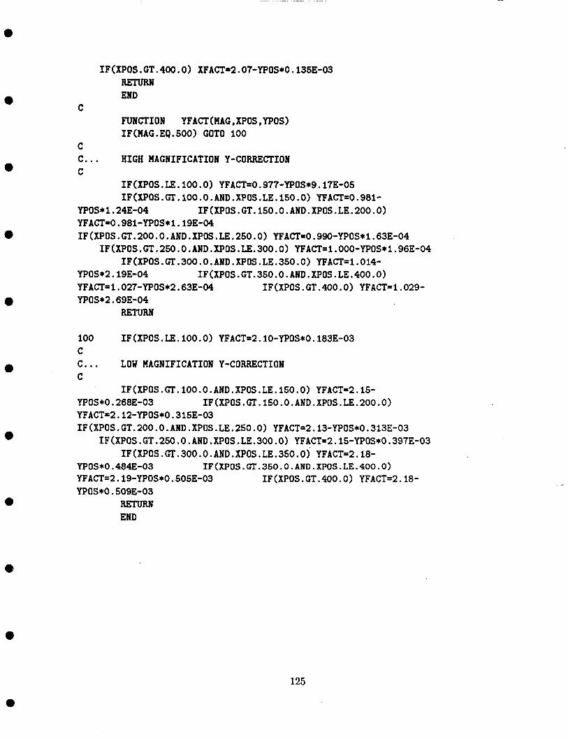
e

e

e

e

0

IF (XPOS . GT. 400.0) XFACT=2.07-YPOS*O. 1353-03 RETURN END

FUNCTION YFACT(MAG,XPOS ,YPOS) IF(MAG . EQ .500) GOT0 100

C

C C... HIGH MAGNIFICATION Y-CORRECTION C

IF(XP0S .LE. 100.0) YFACTsO .977-YPOS*9.17E-05 IF(XP0S .GT . 100 .O .AND. XPOS .LE. 150 .O) YFACTsO .981-

YPOS*1.24E-O4 YFACT=0.98l-YPOS*l.l9E-04 IF (XPOS . GT. 200.0. AND. XPOS . LE. 250.0) YFACTtO .99O-YPOS* 1.63E-04

IF(XP0S .GT. 150.0 .AND .XPOS .LE.200.0)

IF(XPOS.GT.25o.O.AND.XPOS.LE.300.0) YFACT=l.OOO-YPOS*l.96E-04 IF(XP0S. GT. 300.0 .AND. XPOS .LE. 350.0) YFACTtl .014-

YPOS*2.19E-04 IF(XPOS.GT.350.0.AND.XPOS.LE.400.0) YFACT=l.027-YPOS*2.63E-04 IF(XPOS.GT.400.0) YFACT=1.029- YPOS*2.693-04

RETURN

100 IF(XPOS.LE.100.0) YFACT=2.10-YPOS*0.183E-03 C C... LOU MAGNIFICATION Y-CORRECTION C

YPOS*O.268E-O3 YFACT=2.12-YPOS*0,315E-03 IF(XPOS.GT.200.0.AND.XPOS.LE.250.0) YFACT=2.13-YPOS*0.313E-03

IF(XP0S. GT. 100 .O .AND .XPOS .LE. 150 .O) YFACTz2.15- IF(XP0S .GT. 150.0 .AND .XPOS .LE .200 .O)

IF(XPOS.GT.250.0.AND.XPOS.LE.300.0) YFACT=2.15-YPOS*0.397E-03 IF(XP0S .GT.300 .O .AND .XPOS .LE.350.0) YFACTs2.18-

YPOS*O.484E-03 IF(XPOS.GT.350.0.AND.XPOS.LE.400.0) YFACT=2.19-YPOS*0.505E-03 IF (XPOS . GT. 400.0) YFACT=2.18- YPOS*O.509E-03

RETURN END

125

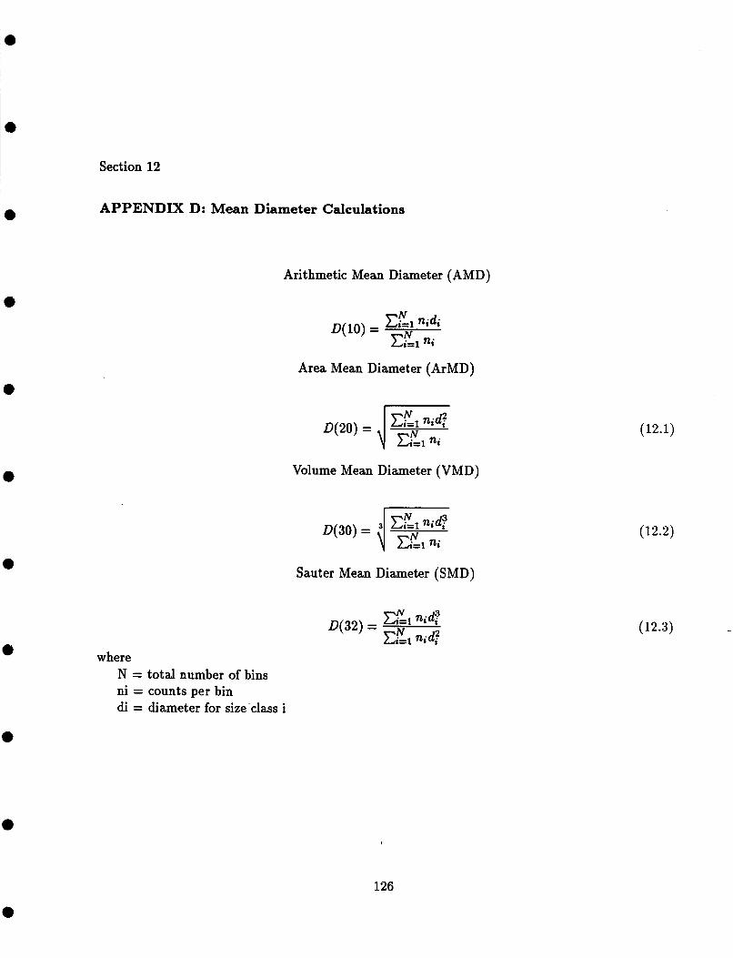
a

Section 12

APPENDIX D: Mean Diameter Calculations

Arithmetic Mean Diameter (AMD)

E21 nidi Cid ni D(10) = N

Area Mean Diameter (ArMD)

e

e

e

0

where N = total number of bins ni = counts per bin di = diameter for size'class i

Volume Mean Diameter (VMD)

Sauter Mean Diameter (SMD)

CEl n;d; xcl n;d?

D(32) =

(12.1)

(12.2)

(12.3) -

126

Section 13

APPENDIX E: Cole-Palmer Flowmeter Calibration Data

Scale Reading 30 40 50 60 70 80 90 100 110 120 130 140

*Calibration values were verified by replication.

Flow-rate (gpm)' 0.022 0.031 0.040 0.050 0.059 0.069 0.078 0.090 0.100 0.110 0.120 0.130

127

a

LI

Y

0.14

e. 12

e. i

. 08

06

. 04

. 02

0

I

A

A

A

A A

A A

A

A

A

A

a

I I I I I I I I 188 1 2 0 140 C 20 40 68 . 88

Flowmeter Scale Reading

Figure 13.1: Cole-Palmer Flowmeter Calibration

128

e

e

a

Section 14

APPENDIX F: OMEGA Pressure Transducer Calibration Data

Table 14.1: S/N: 850502 Standard Pressure Output Voltage Corrected to psia (millivolts)

0 9.20 10 15.00 20 21.70 30 28.30 40 34.80 50 41.45 60 47.95 70 55.20 80 61.70 90 68.60 100 ' 75.20 110 80.70

Table 14.2: OMEGA S/N: 850311 Standard Pressure Output Voltage Corrected to psia (millivolts)

0 9.80 10 16.00 20 22.90 30 29.10 40 35.75 50 42.60 60 49.10 70 56.20 80 62.60 90 69.40 100 75.80 110 81.50

*Calibration values were verified by replication.

129

e

SIN 858502 1 0 0

80

n

.. 28

0

~~

A A

A

A A

A

A

A

A

A

A

20 40 60 80

Standard Preseure ( p s i a )

1 0 0 120

Figure 14.1: OMEGA Pressure Transducer Calibration

130

lee

80

n

> E

60 Y

s e 3 d

0 >

SIN 860311

A A

A

A

A

A

A

I I I I I

Standard Preseure (peia) 0 20 40 60 00 lee 120

Figure 14.2: OMEGA Pressure Transducer Calibration

131

Documents

e FINAL REPORT ON NASA GRANT NAG 3-634 · final report on nasa grant nag 3-634 e “comparison of unl laser imaging and sizing system and a phase/doppler system for analyzing sprays