Embed Size (px)
Citation preview
Effectiveness of Game-Theoretic Strategies inExtensive-Form General-Sum Games
Jirı Cermak1, Branislav Bosansky2, and Nicola Gatti3
1 Dept. of Computer Science, Faculty of Electrical Engineering,Czech Technical University in Prague, Czech Republic,
[email protected] Aarhus University, Aarhus, Denmark,
[email protected] Politecnico di Milano, Milano, Italy,
Abstract. Game theory is a descriptive theory defining the conditionsfor the strategies of rational agents to form an equilibrium (a.k.a. the so-lution concepts). From the prescriptive viewpoint, game theory generallyfails (e.g., when multiple Nash equilibria exist) and can only serve as aheuristic for agents. Extensive-form general-sum games have a plethoraof solution concepts, each posing specific assumptions about the play-ers. Unfortunately, there is no comparison of the effectiveness of thesolution-concept strategies that would serve as a guideline for selectingthe most effective algorithm for a given domain. We provide this com-parison and evaluate the effectiveness of solution-concept strategies andstrategies computed by Counterfactual regret minimization (CFR) andMonte Carlo Tree Search in practice. Our results show that (1) CFRstrategies perform typically the best, (2) the effectiveness of the Nashequilibrium and its refinements is closely related to the correlation be-tween the utilities of players, and (3) that the strong assumptions aboutthe opponent in Strong Stackelberg equilibrium typically cause ineffec-tive strategies when not met.
1 Introduction
One of the most ambitious aims in Multiagent Systems community is the designof artificial agents able to behave optimally in strategic interactions. Well-knownexamples include security domains [27], auctions [29], or classical AI problemssuch as general game-playing [12].
Non-cooperative game theory provides the most elegant mathematical modelsto deal with the strategic interactions. However, in spite of the recent enormoussuccess of its applications, game theory is a descriptive theory describing equi-librium conditions (a.k.a. the solution concepts) for strategies of rational agents(e.g., the best known solution concept Nash equilibrium). On the other hand,game theory may fail when used to prescribe strategies as needed when designingartificial agents (except for specific classes of games, such as strictly competitive
2
games). Failure appears, for example, when multiple Nash equilibria co-exist ina game. Game theory does not specify which Nash equilibrium to choose andplaying strategies from different Nash equilibria may lead to an arbitrarily badutility.4 Other well-known examples of failure are due to the assumptions neededto adopt a given solution concepts that are rarely met (e.g., player 2 breakingties in favor of player 1 in Strong Stackelberg equilibrium).
The following question thus naturally appears: Is it meaningful to follow pre-scribed game-theoretic strategies in an actual game play regardless of the lack ofthe theoretical guarantees? We experimentally investigate this question, focusingon general-sum two-player finite extensive-form games (EFGs) with imperfectinformation and uncertainty, since they offer a general representation of sequen-tial interaction of two players with differing preferences, commonly found in realworld scenarios (e.g., security scenarios where thieves value items differently thanguards). EFGs have been a subject of a long-term research from the perspectiveof game theory and there is a large collection of solution concepts defined for thisclass of games. Nash equilibrium is considered to be a weak solution concept inEFGs since it can use non-credible threats and prescribe irrational actions (weprovide an example in the following sections). Therefore, several refinements ofNash equilibria have been introduced over the years posing additional constraintsover the strategies to rule out undesirable equilibria. In particular, we investigatethe refinements undominated equilibrium [8] and Quasi-Perfect equilibrium [7],since we are interested in the correlation between increasing theoretical guar-antees and practical effectiveness of strategies. Furthermore we evaluate Nashequilibria that maximize expected utility of a given player, or sum of the expectedutilities of both players. While refinements remove some undesirable equilibria,they do not resolve the main issue of game-theoretic solution concepts and donot guarantee the expected outcome. To obtain guarantees, one can use maximin(prudential) strategies that maximize the expected outcome in the worst caseby assuming that the opponent is playing to hurt the player the most, with acomplete disregard of his own gains. However, this assumption is often too pes-simistic. Alternatively, strategies that are the outcome of a learning algorithmare often used in practice. Two types of learning algorithms are well-establishedin EFGs: Counterfactual Regret Minimization (CFR; [30]) and Monte Carlo TreeSearch (MCTS; [13]). Although none of these algorithms have any guaranteesto converge to a game-theoretic solution in general-sum games, they are bothwidely used (e.g., [23, 10]), since this lack of theory does not necessarily weakentheir usefulness as game theory does not provide any guarantees either.
In this paper we provide a thorough experimental comparison of the strategiesthat are either described by various solution concepts, or that are a result of alearning algorithm. We measure their effectiveness as an expected utility valueof player 1 against some strategy of player 2 on a set of games with differingcharacteristics. A similar analysis has been previously conducted only on zero-sum extensive-form games [31], where Nash equilibrium strategies are guaranteed
4Let us note that Nash equilibrium would be not the appropriate solution concept if the commu-nication before playing is available.
3
to achieve at least the value of the game. Interestingly, our results show that themost effective strategies are the outcomes of the CFR algorithm that typicallyoutperform all other strategies. The CFR is widely used in poker domain, but asour results show, the CFR strategies are effective and robust beyond the domainof poker. The effectiveness of the strategies based on Nash equilibria typicallyvaries with the correlation factor between the evaluation of the players (i.e.,whether the players are adversarial, or cooperative). Finally, using additionalassumptions about the opponent common in solution concepts can result in loweffectiveness of the strategies when these assumptions are not met.
2 Technical Background
We focus on general-sum extensive-form games (EFGs) that can be visualizedas game trees (see Fig. 1). Each node in the game tree corresponds to a non-terminal state of the game, in which one player is making a move (an edge inthe game tree) leading to another state of the game. We restrict to two-playerEFGs, where P = {1, 2} is the set of players. We use i to denote a player and−i to denote the opponent of i. Utility function ui that players aim to maximizeassigns a value for every terminal state (leaf in the tree).
The imperfect information is defined using the information sets (the dashedellipses in Fig. 1). States grouped in a single information set are indistinguishableto player acting in these states. We assume perfect recall, where the playersperfectly remember the history of their actions and all observed information.
A pure strategy si for player i is a mapping of an action to play to eachinformation set assigned to player i. Si is a set of all pure strategies for playeri. A mixed strategy δi is a distribution over Si, set of all mixed strategies of i isdenoted as ∆i. When players follow a pair of strategies, we again use ui to denotethe expected utility of player i. We say that strategy si weakly dominates s′i iff∀s−i ∈ S−i : ui(si, s−i) ≥ ui(s′i, s−i) and ∃s−i ∈ S−i : ui(si, s−i) > ui(s
′i, s−i).
Strategies can be represented as behavioral strategies Bi in EFGs, wherea probability distribution is assigned over the actions in each information set.Behavioral strategies have the same expressive power as mixed strategies ingames with perfect recall [18], but can be more compactly represented usingthe sequence-form representation [14]. A sequence is a list of actions of player iordered by their occurrence on the path from the root of the game tree to somenode. A strategy is then formulated as a realization plan ri that for a sequencerepresents the probability of playing actions in this sequence assuming the otherplayers play such that this actions can be executed.
3 Overview of Solution Concepts
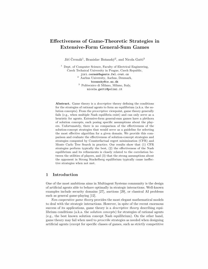
We now provide an overview of the analyzed solution concepts. As a runningexample we use the game from Fig. 1. The game starts by dealing 1 secret cardon the table. Player 1 moves next and decides between (i) action E endingthe game right now leading to the immediate outcome 0 for both players, (ii)
4
Fig. 1. Example of a EFG termed Informer’s Ace of Spades.
showing the player 2 the card dealt H, and (iii) letting player 2 guess withoutany information C. If player 1 lets player 2 guess, the game reaches a statewhere player 2 tries to guess whether the hidden card is Ace of spades (As) ornot (nAs). A correct guess yields outcome of 4 for player 2, while player 1 gets−1. If player 2 guesses incorrectly both players get 0. If player 1 tells player 2which card has been dealt, the game proceeds to a state where player 2 decideswhether to be selfish (actions S, S′ leading to outcomes (0, 3)), or to be generousand reward player 1 (actions G, G′ leading to outcomes (1, 2)).
Nash Equilibrium. The concept of Nash equilibrium (NE) is based on thenotion of best response. A best response (BR) to a strategy of the opponent δ−iis a strategy δ∗i for which ui(δ
∗i , δ−i) ≥ ui(δi, δ−i), ∀δi ∈ ∆i. We denote the set
of the BRs to the strategy δ−i as BRi(δ−i). We say that strategy profile {δi, δ−i}is a NE iff δi ∈ BRi(δ−i), ∀i ∈ P . A game can have more than one NE.
The game from Fig. 1 has 4 pure strategy NE {{(H), (E)} × {(S, S′, As),(S, S′, nAs)}}. Our example shows why NE is a weak solution concept in EFGs.Some of the NE strategy profiles are not reasonable – for example, playing Asfor player 2, since the appearance of any other card is more probable. However,playing As is consistent with NE conditions, since player 2 does not expectthe information set after action C to be reached as C is not a part of any NEstrategy of player 1. Playing E over H is also unreasonable, since player 1 cannever lose by preferring H over E (H weakly dominates E). However since anyrational player 2 will play S and S′ there is, according to NE, nothing to gainby preferring H over E.
Sequential Equilibrium. The sequential equilibrium (SE) due to Kreps andWilson [16] is the natural refinement of Subgame Perfect equilibrium for gameswith imperfect information. SE uses a notion of beliefs µ, which are probabilitydistributions over the states in information sets symbolizing the likeliness ofbeing in a state when the information set is reached. Assessment is a pair (µ,B)
5
representing beliefs for all players and a behavioral strategy profile. A SE is anassessment which is consistent (µ is generated by B) and sequential best responseagainst itself (B is created by BRs when considering µ). The set of SE forms anon-empty subset of NE [16].
The set of SE of the game from Fig. 1 is {{(H), (E)} × {(S, S′, nAs)}}. TheSE eliminated the NE that contained the action As, since the SE reasons aboutthe action As and nAs with the additional knowledge of beliefs over the gamestates in the information set. Since the probability of being in the state whereace of spades was dealt is smaller than the opposite, SE rules out the action As.
Undominated Equilibrium. An undominated equilibrium (UND) is a NEusing only undominated strategies in the sense of weak dominance. For two-player EFGs it holds that every UND of EFG G is a perfect equilibrium (asdefined by Selten [24]) of its corresponding normal-form game G′ and thereforeforms a Normal-form perfect equilibrium of G. The set of UND forms a non-empty subset of NE [24].
The UND of the game from Fig. 1 are {{(H)} × {(S, S′, As), (S, S′, nAs)}}.UND removed two NE where player 1 plays E, since H weakly dominates E.
Quasi-Perfect Equilibrium. Informally speaking, Quasi-Perfect equilibrium(QPE) is a solution concept due to van Damme [7] that requires that each playerat every information set takes a choice which is optimal against mistakes of allother players. The set of all QPE forms a non-empty subset of intersection ofSE and UND [7].
The only QPE of the game in Fig. 1 is {(H), (S, S′, nAs)}, as it is the NElying in the intersection of UND and SE.
Outcome Maximizing Equilibria. Besides refinements of NE, it is commonthat agents follow specific NE strategy based on the expected utility outcome.We use two examples of such specific NE: (1) we use player 1 outcome maximiz-ing equilibrium (P1MNE) and (2) welfare equilibrium (WNE), which is a NEmaximizing the sum of expected utilities of both players.
The set of P1MNE of the game from Fig. 1 is equal to the set of NE since allthe NE generate the same expected value for player 1. The set of WNE of thegame from Fig. 1 is {{(H)} × {(S, S′, As), (S, S′, nAs}}.
Stackelberg Equilibrium. The Stackelberg equilibrium assumes player 1 totake the role of a leader while player 2 plays a follower. Leader commits toa strategy δl observed by the follower. The follower then proceeds to play apure BR to δl. The pair of strategies (δl, g(δl)), where g(δl) is a follower bestresponse function g : ∆l → Sf , is said to be a Stackelberg equilibrium iffδl ∈ arg maxδ′l∈∆l
ul(δ′l, g(δ′l)) and uf (δ′l, g(δ′l)) ≥ uf (δ′l, g
′(δ′l)),∀g′, δ′l. When g
breaks ties optimally for the leader, the pair (δl, g(δl)) forms a Strong Stackelbergequilibrium (SSE) [19, 4].
6
The set of SSE of the game from Fig. 1 is {{(H)}×{(S, S′, As), (S, S′, nAs)}}∪{{(E)} × {(S, S′, As), (S, S′, nAs), (S,G′, As), (S,G′, nAs)}}.
4 Computing Strategies
We now focus on the algorithms for computing the solution concepts. Computingdifferent solution concepts has different computational complexity; it is PPAD-complete to compute one NE [9], QPE [22] and UND [26], while it is NP-hardto compute some specific NE (i.e., WNE, P1MNE) [5] and SSE [20].
4.1 Computing Game-Theoretic Strategies
We describe the algorithms used to compute NE, UND, P1MNE, WNE, QPE,SSE and maximin strategies in this order. Due to the space constraints we onlydescribe the key idea behind the algorithm. The baseline algorithm is the LCPformulation due to Koller et al. [15], which guarantees all its feasible solutionsto be NE. LCP formulation, however, does not allow us to choose some specificNE (e.g., required for UND, WNE, P1MNE). Therefore, we also use a MILPreformulation of the LCP obtained by linearisation of the complementarity con-straints [1].
(1) NE is computed by LCP formulation due to Koller et al. [15].(2) UND is computed by using the MILP formulation [1] maximizing r>1 U1r
m2 ,
where rm2 is a uniform strategy of the player 2. This objective ensures findingNE that is a BR to a fully mixed strategy. By definition of dominance, such aNE cannot contain dominated strategies and thus it is a UND [8].
(3) WNE is computed by using the MILP formulation [1] maximizing thesum of expected values of both players.
(4) P1MNE is computed by using the MILP formulation [1] maximizing theexpected value of player 1.
(5) QPE is computed using a LCP with symbolic perturbation in ε. The per-turbation model used in this paper to produce QPE is due to Miltersen et al. [22].It restricts the strategies in the game by requiring every sequence σi for all play-ers to be played with a probability at least ε|σi|+1 where |σi| is the length of σi.All the feasible solutions of the perturbed LCP are guaranteed to be QPE.
(6) SSE is computed by the MILP formulation due to Bosansky et al. [3].(7) Maximin strategies are computed using the LP formulation for finding NE
of zero-sum games due to Koller et al. [14] from the perspective of player 1. Thestrategy resulting from this LP is guaranteed to be maximin, as this formulationassumes player 2 to have the utilities exactly opposite to the utilities of player 1.By maximizing her expected outcome, player 2 minimizes the expected outcomeof player 1 and therefore behaves as the worst case opponent.
4.2 Counterfactual Regret Minimization (CFR)
CFR due to Zinkevich et al. [30] iteratively traverses the whole game tree, up-dating the strategy with an aim to minimize the overall regret. The overall regret
7
is bounded from above by the sum of additive regrets (counterfactual regrets,defined for each information set), which can be minimized independently.
4.3 Monte Carlo Tree Search (MCTS)
MCTS is an iterative algorithm that uses a large number of simulations whileiteratively building the tree of the most promising nodes. We use the most typi-cal game-playing variant: UCB algorithm due to Kocsis et al. [13] is used as theselection method in each information set (Information Set MCTS [6]). Addition-ally we use nesting [2]—MCTS algorithm runs for a certain number of iterations,then advances to each of the succeeding information sets and repeats the wholeprocedure. This method ensures that all parts of the game tree are visited oftenenough so that the frequencies, with which the MCTS algorithm selects the ac-tions in this information set, better approximate the optimal behavioral strategy.Moreover, using nesting simulates online decision making, where the players aremaking the decision in a limited time in each information set.
5 Experiments
We now describe the main results of the paper and provide the comparison of theeffectiveness of the different strategies in EFGs – i.e., we assume that player 1 isusing a strategy prescribed by some solution concept, or an iterative algorithm,and we are interested in the expected outcome for player 1 against some strategyof player 2. We first describe the domains used for the comparison that includerandomly generated games and simplified general-sum poker. Since finding a NE(especially some specific equilibrium) in general-sum games is a computationallyhard problem, we follow with the experimental evaluation of the scalability ofthe algorithms. Next we describe the opponents (strategies for player 2) used forthe strategy effectiveness experiments. Finally we measure the effectiveness ofstrategies against the NE minimizing expected utility of player 1.
5.1 Domains
There is no set of standard benchmark domains available to measure the ef-fectiveness of strategies in general sum EFGs. We try to create such a set byusing games with differing characteristics to provide as thorough evaluation ofthe strategies as possible. We primarily use randomly generated games, sincethey provide variable sources of uncertainty for the players and we can alterthe properties of the games (e.g., utility correlation factor) to investigate thesensitivity to different characteristics. On the other hand, we also use simplifiedpoker games since they are widely used for benchmark purposes, even thoughthey are limited in terms of uncertainty that is only caused by the unobservableaction of nature at the beginning of the game.
8
Extended Kuhn Poker. Extended Kuhn poker is a modification of the pokervariant Kuhn poker [17]. In Extended Kuhn poker the deck contains only 3 cards{J,Q,K}. The game starts with a non-optional bet of 1 called ante, after whicheach of the players receives a single card and a betting round begins. In thisround player 1 decides to either bet, adding 1 to the pot, or to check. If he bets,second player can either call, adding 1 to the pot, raise adding 2 to the pot orfold which ends the game in the favor of player 1. If player 1 checks, player 2 caneither check or bet. If player 2 raises after a bet, player 1 can call or fold endingthe game in the favor of player 2. This round ends by call or by check from bothplayers. After the end of this round, the cards are revealed and the player withthe bigger card wins the pot. Our games are general-sum assuming that 10% ofthe pot is claimed by the dealer regardless of the winner. Furthermore there arebounties assigned to specific cards, paid when player wins with such card.
Leduc Holdem Poker. Leduc holdem poker [25] is a more complex variant ofa simplified poker. The deck contains {J, J,Q,Q,K,K}. The game starts as inExtended Kuhn. After the end of the first betting round one card is dealt on thetable. Second betting round with the same rules begins. After the second bettinground, the outcome of the game is determined. A player wins if (1) her privatecard matches the table card, or (2) none of the players’ cards matches the tablecard and her private card is higher than the private card of the opponent. If noplayer wins, the pot is split. As before, 10% of the pot is claimed by the dealer.Furthermore there are bounties assigned to specific card combinations.
Randomly Generated Games. Finally, we use randomly generated gameswithout nature. We alter several characteristics of the games: the depth of thegame (number of moves for each player), the branching factor representing thenumber of actions in each information set; number of observation signals gener-ated by the actions (each action of a player generates observation signal, repre-sented as a number from a limited set, for the opponent—the states that sharethe same history and the sequence of observations belong to the same infor-mation set). The utility for player 1 is uniformly generated from the interval[−100, 100]. The utility of player 2 is computed based on the correlation param-eter from [−1, 1]. Correlation set to 1 leads to identical utilities, −1 to a zero-sumgame. Otherwise, the utility of player 2 is uniformly generated from a restrictedinterval around the multiplication of utility of player 1 and the correlation factor.
5.2 Scalability Results
Table 1 provides the computation times (in milliseconds) it takes to compute theequilibrium strategies. Presented numbers are means of 50 runs of different ran-domly generated games of fixed size. We used Lemke algorithm implementationin C language using unlimited precision arithmetic to compute QPE (similarto [11]), IBM CPLEX 12.5.1 was used to compute all the MILP-based solutionconcepts.
9
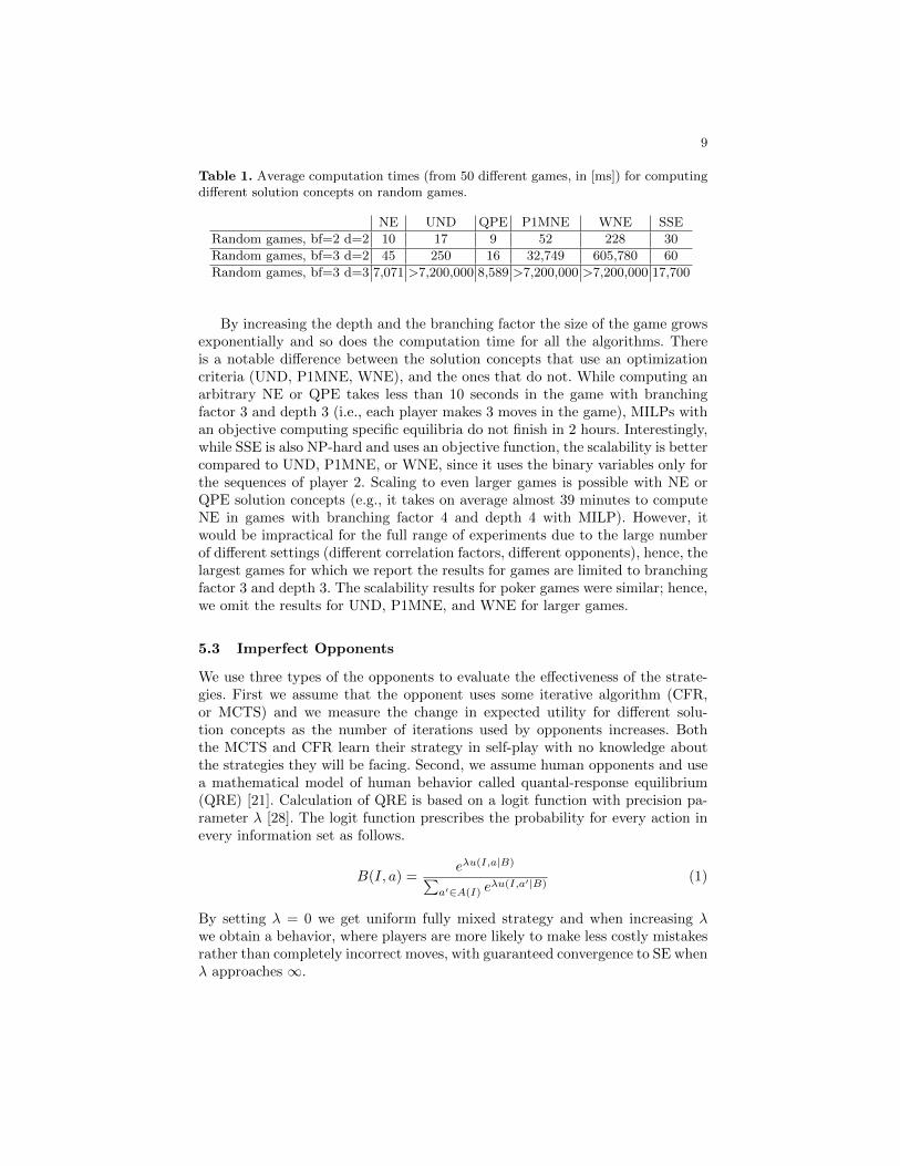
Table 1. Average computation times (from 50 different games, in [ms]) for computingdifferent solution concepts on random games.
NE UND QPE P1MNE WNE SSE
Random games, bf=2 d=2 10 17 9 52 228 30
Random games, bf=3 d=2 45 250 16 32,749 605,780 60
Random games, bf=3 d=3 7,071 >7,200,000 8,589 >7,200,000 >7,200,000 17,700
By increasing the depth and the branching factor the size of the game growsexponentially and so does the computation time for all the algorithms. Thereis a notable difference between the solution concepts that use an optimizationcriteria (UND, P1MNE, WNE), and the ones that do not. While computing anarbitrary NE or QPE takes less than 10 seconds in the game with branchingfactor 3 and depth 3 (i.e., each player makes 3 moves in the game), MILPs withan objective computing specific equilibria do not finish in 2 hours. Interestingly,while SSE is also NP-hard and uses an objective function, the scalability is bettercompared to UND, P1MNE, or WNE, since it uses the binary variables only forthe sequences of player 2. Scaling to even larger games is possible with NE orQPE solution concepts (e.g., it takes on average almost 39 minutes to computeNE in games with branching factor 4 and depth 4 with MILP). However, itwould be impractical for the full range of experiments due to the large numberof different settings (different correlation factors, different opponents), hence, thelargest games for which we report the results for games are limited to branchingfactor 3 and depth 3. The scalability results for poker games were similar; hence,we omit the results for UND, P1MNE, and WNE for larger games.
5.3 Imperfect Opponents
We use three types of the opponents to evaluate the effectiveness of the strate-gies. First we assume that the opponent uses some iterative algorithm (CFR,or MCTS) and we measure the change in expected utility for different solu-tion concepts as the number of iterations used by opponents increases. Boththe MCTS and CFR learn their strategy in self-play with no knowledge aboutthe strategies they will be facing. Second, we assume human opponents and usea mathematical model of human behavior called quantal-response equilibrium(QRE) [21]. Calculation of QRE is based on a logit function with precision pa-rameter λ [28]. The logit function prescribes the probability for every action inevery information set as follows.
B(I, a) =eλu(I,a|B)∑
a′∈A(I) eλu(I,a′|B)
(1)
By setting λ = 0 we get uniform fully mixed strategy and when increasing λwe obtain a behavior, where players are more likely to make less costly mistakesrather than completely incorrect moves, with guaranteed convergence to SE whenλ approaches ∞.
10
Finally, we assume that the opponent is computing NE, however, we do notknow which NE will be selected. Therefore, we are interested in the expectedvalue of player 1 against NE strategy of player 2 that minimizes the expectedvalue of player 1 (i.e., the worst case out of all NE strategies player 2 can select).
5.4 Measuring the Effectiveness of Strategies
We present the relative effectiveness of the strategies. The upper and lowerbound on the value are formed by the best and the worst response of player1 against strategy of player 2 (relative effectiveness is equal to 1 if the strategyobtains the same expected utility as the best response, 0 if it obtains the sameexpected utility as the worst response). We use the relative values to eliminatethe inconsistency caused by randomly generated utility values.
Where possible (due to computation-time constraints), we show the relativeeffectiveness within an interval for best and worst NE strategies—i.e., we use aMILP formulation for computing NE and maximize (or minimize) the expectedutility value of player 1 against the specific strategy of player 2. This intervalcontains all NE and its refinements and it is visualized as a grey area in theresults. Finally, we use 105 iterations of CFR and MCTS algorithms to producethe strategies of player 1 (both algorithms learn in self play with no informationabout the strategies they will face) used for the effectiveness comparison.
5.5 Results
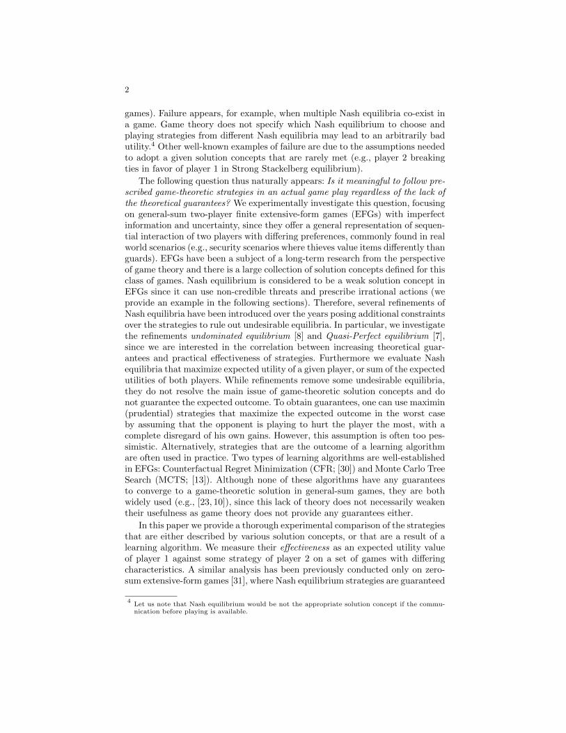
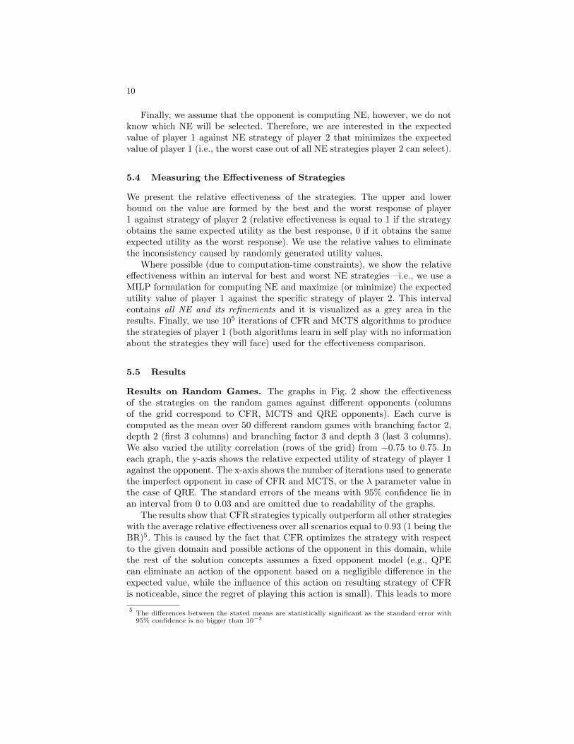
Results on Random Games. The graphs in Fig. 2 show the effectivenessof the strategies on the random games against different opponents (columnsof the grid correspond to CFR, MCTS and QRE opponents). Each curve iscomputed as the mean over 50 different random games with branching factor 2,depth 2 (first 3 columns) and branching factor 3 and depth 3 (last 3 columns).We also varied the utility correlation (rows of the grid) from −0.75 to 0.75. Ineach graph, the y-axis shows the relative expected utility of strategy of player 1against the opponent. The x-axis shows the number of iterations used to generatethe imperfect opponent in case of CFR and MCTS, or the λ parameter value inthe case of QRE. The standard errors of the means with 95% confidence lie inan interval from 0 to 0.03 and are omitted due to readability of the graphs.
The results show that CFR strategies typically outperform all other strategieswith the average relative effectiveness over all scenarios equal to 0.93 (1 being theBR)5. This is caused by the fact that CFR optimizes the strategy with respectto the given domain and possible actions of the opponent in this domain, whilethe rest of the solution concepts assumes a fixed opponent model (e.g., QPEcan eliminate an action of the opponent based on a negligible difference in theexpected value, while the influence of this action on resulting strategy of CFRis noticeable, since the regret of playing this action is small). This leads to more
5The differences between the stated means are statistically significant as the standard error with95% confidence is no bigger than 10−3
11
�������������� ������ �� ��� ���� ���
branching factor 2, depth 2 branching factor 3, depth 3QRE MCTS CFR QRE MCTS CFR
corr
.-0
.75
10�3 100 103
0.7
0.8
0.9
1
0 1000 20000.7
0.8
0.9
1
0 500 1000
0.8
0.9
1
10�3 100 103
0.7
0.8
0.9
1
0 10000 200000.7
0.8
0.9
1
0 5000 100000.8
0.85
0.9
0.95
1
corr
.-0
.25
10�3 100 103
0.6
0.8
1
0 1000 2000
0.6
0.8
1
0 500 1000
0.6
0.8
1
10�3 100 103
0.7
0.8
0.9
1
0 10000 200000.5
0.6
0.7
0.8
0.9
0 5000 10000
0.7
0.8
0.9
1
corr
.0.2
5
10�3 100 103
0.4
0.6
0.8
1
0 1000 2000
0.4
0.6
0.8
1
0 500 1000
0.4
0.6
0.8
1
10�3 100 1030.4
0.6
0.8
1
0 10000 200000.5
0.6
0.7
0.8
0.9
0 5000 100000.4
0.6
0.8
1
corr
.0.7
5
10�3 100 1030
0.2
0.4
0.6
0.8
1
0 1000 2000
0.2
0.4
0.6
0.8
1
0 500 1000
0.2
0.4
0.6
0.8
1
10�3 100 1030.4
0.6
0.8
1
0 10000 20000
0.7
0.8
0.9
1
0 5000 100000.4
0.6
0.8
1
λ iterations iterations λ iterations iterations
Fig. 2. Relative effectiveness of the strategies computed as a mean over 50 randomgames with the b.f. 2, d. 2 (columns 1-3) and b.f. 3, d. 3 (columns 4-6) and varyingutility correlation against imperfect opponents
effective CFR strategies, especially in competitive scenarios (see the first row inFig. 2, where correlation is set to −0.75).
MCTS was the second best with the mean of 0.9, however, its effectivenessis not consistently close to the best. It is weak, e.g., against the CFR opponenton random games with depth 3, branching factor 3 and correlation -0.75 (firstrow last graph in Fig. 2). On the other hand, it has the best effectiveness, e.g.,against the QRE opponent on random games with depth 3, branching factor 3and correlation 0.25 (third row fourth graph).
In games with negative utility correlation the QPE strategies perform well,often very close to CFR (first row in Fig. 2), with the overall mean value equalto 0.85. This is due to the fact that the QPE tries to exploit the mistakes of theopponent. If the correlation is negative, the mistakes of player 2 very likely helpplayer 1, and thus their exploitation significantly improves the expected utility.However as the correlation factor increases the advantages player 1 can get fromthe mistakes of the player 2 diminish, since the mistakes of player 2 decreasealso the utility for player 1, and so the effectiveness of QPE decreases (last rowin Fig. 2).
12
�� ��� ��� ��� ���� �� �� ��� ��
c. -0.75 c. -0.25 c. 0.25 c. 0.75
0.86
0.88
0.9
0.92
0.94
0.96
0.4
0.5
0.6
0.7
0.2
0.3
0.4
0.5
0.6
0.2
0.3
0.4
0.5
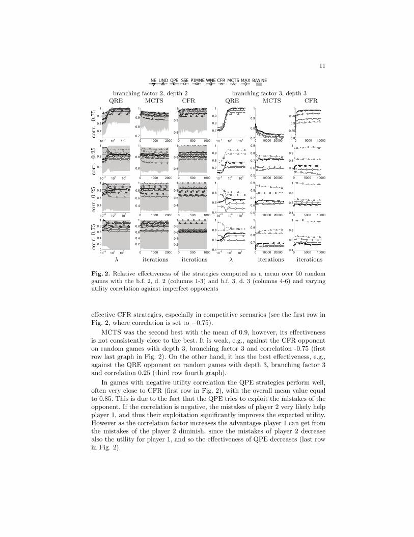
Fig. 3. Confidence intervals depicting the relative expected effectiveness of the mea-sured strategies against the NE minimizing expected value of every measured strategyon random games with b.f. 2 and depth 2
UND strategies are often the worst for the negative correlation (first rowin Fig. 2), but their effectiveness increases with higher correlation (last row inFig. 2). This is because we compute UND using uniform strategy of the opponentin the objective of MILP; hence, the strategy of player 1 is trying to reachleafs with high outcome through the whole game tree. As the utility correlationincreases, there is a higher chance that player 2 will try to reach the same leafs.
The NE and its modifications WNE and P1MNE achieve inconsistent effec-tiveness through the experiments, because their only guarantee is against a fixedstrategy of the opponent resulting from the MILP computation. They performwell only if the opponent strategy approximates the strategy computed by theMILP. The results from Fig. 2 show that WNE and P1MNE tend to score bet-ter for highly correlated utilities, because the utilities of players are likely to besimilar and so there is a higher chance that the opponent will fit to the modelassumed and will try to reach the expected nodes.
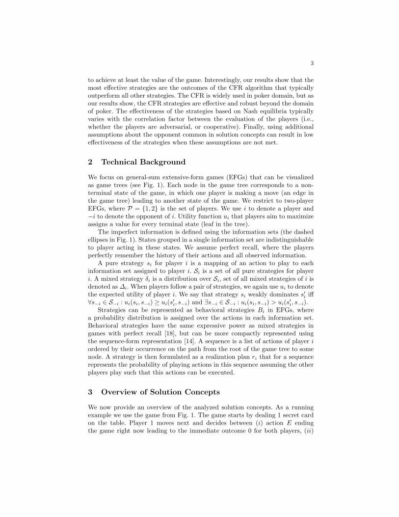
While maximin strategies provide guarantees in the worst case scenario, theyuse very pessimistic assumptions about the opponent, assuming that he will aimto hurt player 1 as much as possible with complete disregard of his own gains.Figure 2 shows that the maximin strategies have typically very bad effectiveness,with the exception of random games with negative utility correlation, since thelower the utility correlation, the closer we are to zero-sum games where themaximin strategies form a NE. On the other hand, we compare the effectivenessof the strategies against the NE strategy of player 2 that minimizes the expectedvalue of player 1 (Fig. 3 shows the mean of relative expected values of player 1with 95% confidence intervals showing the standard error against this strategy).The worst case NE opponent is close to the maximin assumptions; hence, themaximin strategies have the highest effectiveness of all (except for the case ofcorrelation equal to -0.75, where all strategies scored similarly), proving theusefulness of worst case guarantees in this setting (UND was the second bestfollowed by CFR).
Finally, the effectiveness of SSE is typically the worst out of all comparedstrategies, with the relative mean equal to 0.77. This is caused by the fact thatthe leader assumes the follower to observe his strategy, and so the leader can
13
�������������� ������ �� ��� ���� ���
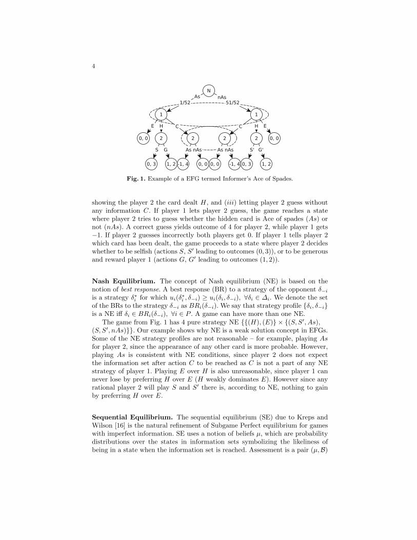
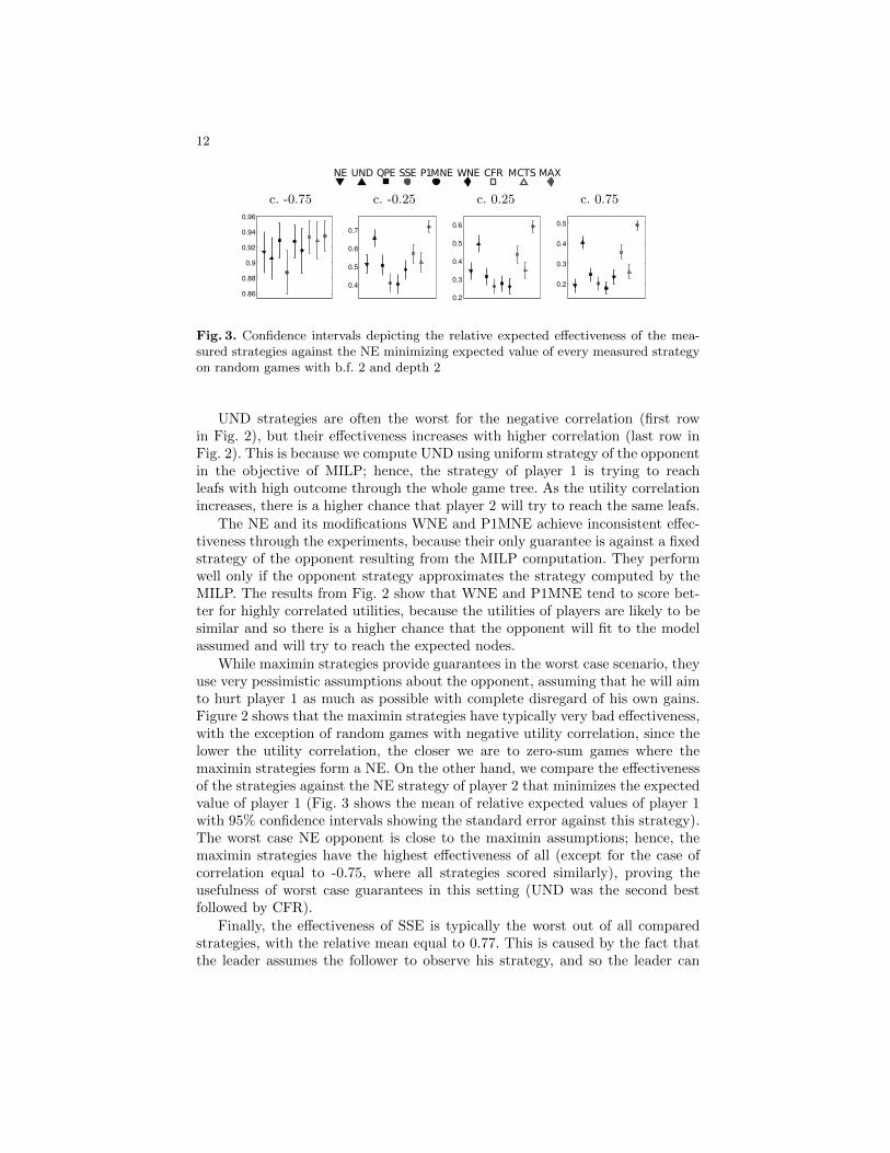
Extended Kuhn Leduc holdemQRE MCTS CFR QRE MCTS CFR
100 103 106
0.7
0.8
0.9
1
0 2000 40000.7
0.8
0.9
0 1000 2000
0.8
0.9
1
10�3 100 1030.4
0.6
0.8
1
0 5000 100000.5
0.6
0.7
0.8
0.9
0 10000 200000.4
0.6
0.8
1
λ iterations iterations λ iterations iterations
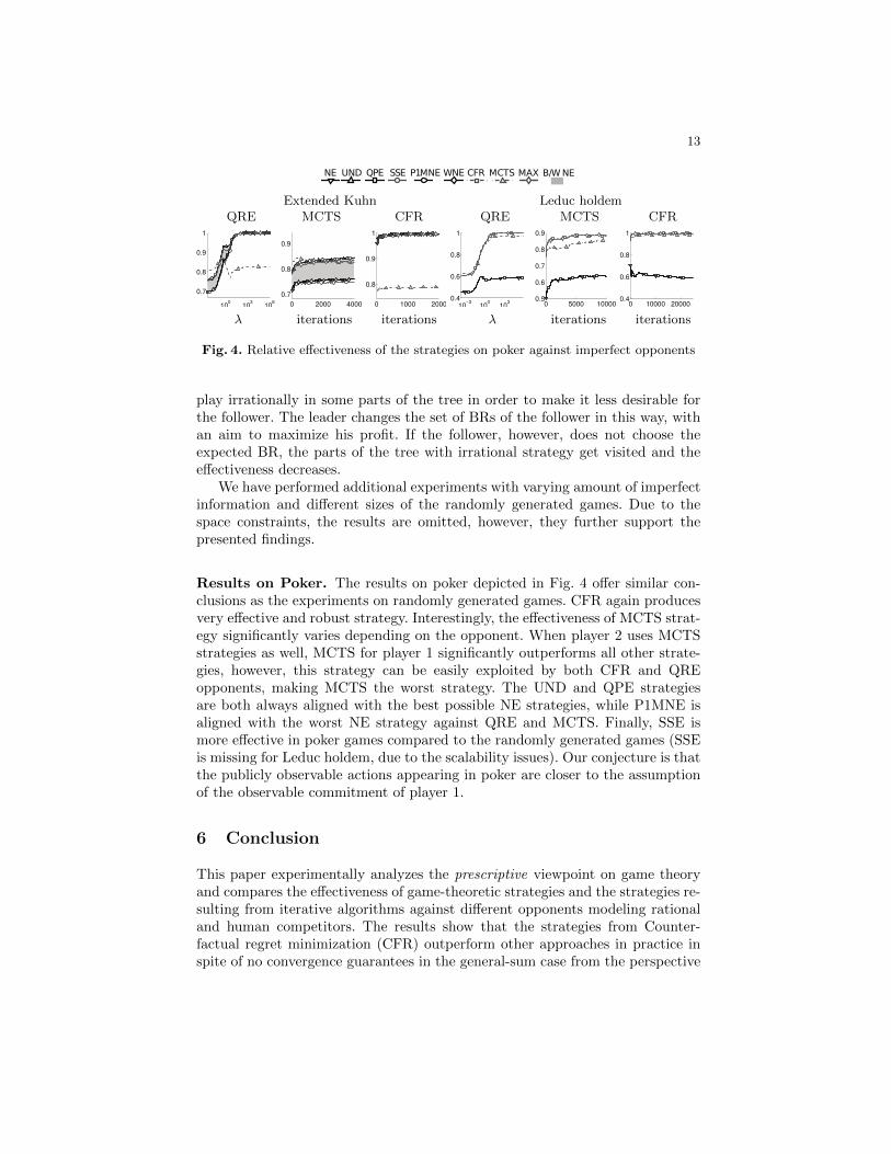
Fig. 4. Relative effectiveness of the strategies on poker against imperfect opponents
play irrationally in some parts of the tree in order to make it less desirable forthe follower. The leader changes the set of BRs of the follower in this way, withan aim to maximize his profit. If the follower, however, does not choose theexpected BR, the parts of the tree with irrational strategy get visited and theeffectiveness decreases.
We have performed additional experiments with varying amount of imperfectinformation and different sizes of the randomly generated games. Due to thespace constraints, the results are omitted, however, they further support thepresented findings.
Results on Poker. The results on poker depicted in Fig. 4 offer similar con-clusions as the experiments on randomly generated games. CFR again producesvery effective and robust strategy. Interestingly, the effectiveness of MCTS strat-egy significantly varies depending on the opponent. When player 2 uses MCTSstrategies as well, MCTS for player 1 significantly outperforms all other strate-gies, however, this strategy can be easily exploited by both CFR and QREopponents, making MCTS the worst strategy. The UND and QPE strategiesare both always aligned with the best possible NE strategies, while P1MNE isaligned with the worst NE strategy against QRE and MCTS. Finally, SSE ismore effective in poker games compared to the randomly generated games (SSEis missing for Leduc holdem, due to the scalability issues). Our conjecture is thatthe publicly observable actions appearing in poker are closer to the assumptionof the observable commitment of player 1.
6 Conclusion
This paper experimentally analyzes the prescriptive viewpoint on game theoryand compares the effectiveness of game-theoretic strategies and the strategies re-sulting from iterative algorithms against different opponents modeling rationaland human competitors. The results show that the strategies from Counter-factual regret minimization (CFR) outperform other approaches in practice inspite of no convergence guarantees in the general-sum case from the perspective
14
of game theory. Among the strategies prescribed by the game-theoretic solutionconcepts, the effectiveness often depends on the utility structure of the game.In case the utility functions of players are positively correlated, strategies ofUndominated equilibrium provide an effective and robust choice. In case of neg-ative correlation, strategies of Quasi-Perfect equilibrium effectively exploit themistakes of the opponent and thus provide a good expected outcome. Finally,our results show that strong assumptions about its opponent made by StrongStackelberg equilibrium cause ineffective strategies when these assumptions arenot met in actual experiments.
This paper opens several directions for future work. Our results show thatCFR strategies are effective beyond the computational poker, but there is an ap-parent lack of theory that would formally explain the empirical success of CFRstrategies in general-sum sequential games. Next, our experiments were limitedby the scalability of the current algorithms for computing different solution con-cepts and the results might differ with increasing sizes of the games. Therefore,new algorithms that allow scaling to larger games need to be designed in orderto confirm our findings for more realistic games.
Acknowledgements. This research was supported by the Czech Science Foun-dation (grant no. P202/12/2054 and 15-23235S), by the Danish National Re-search Foundation and The National Science Foundation of China (under thegrant 61361136003) for the Sino-Danish Center for the Theory of InteractiveComputation. Access to computing and storage facilities owned by parties andprojects contributing to the National Grid Infrastructure MetaCentrum, pro-vided under the programme ”Projects of Large Infrastructure for Research, De-velopment, and Innovations” (LM2010005), is greatly appreciated.
References
1. Audet, C., Belhaiza, S., Hansen, P.: A new sequence form approach for the enu-meration and refinement of all extreme Nash equilibria for extensive form games.International Game Theory Review 11 (2009)
2. Baier, H., Winands, M.H.M.: Nested Monte-Carlo Tree Search for Online Planningin Large MDPs. In: ECAI (2012)
3. Bosansky, B., Cermak, J.: Sequence-Form Algorithm for Computing StackelbergEquilibria in Extensive-Form Games. In: AAAI (2015)
4. Conitzer, V., Sandholm, T.: Computing the optimal strategy to commit to (2006)5. Conitzer, V., Sandholm, T.: New complexity results about Nash equilibria. Games
and Economic Behavior 63(2), 621 – 641 (2008)6. Cowling, P.I., Powley, E.J., Whitehouse, D.: Information Set Monte Carlo Tree
Search. Computational Intelligence and AI in Games, IEEE Transactions on 4,120–143 (2012)
7. van Damme, E.: A relation between perfect equilibria in extensive form games andproper equilibria in normal form games. Game Theory 13, 1–13 (1984)
8. van Damme, E.: Stability and Perfection of Nash Equilibria. Springer-Verlag (1991)
15
9. Daskalakis, C., Fabrikant, A., Papadimitriou, C.H.: The Game World Is Flat: TheComplexity of Nash Equilibria in Succinct Games. In: ICALP. pp. 513–524 (2006)
10. Finnsson, H., Bjornsson, Y.: Simulation-based approach to general game-playing.In: AAAI. pp. 259–264 (2008)
11. Gatti, N., Iuliano, C.: Computing an extensive-form perfect equilibrium in two-player games. In: AAAI (2011)
12. Genesereth, M., Love, N., Pell, B.: General game-playing: Overview of the AAAIcompetition. AI Magazine 26, 73–84 (2005)
13. Kocsis, L., Szepesvari, C., Willemson, J.: Improved Monte-Carlo Search. Tech. Rep1 (2006)
14. Koller, D., Megiddo, N., von Stengel, B.: Fast algorithms for finding randomizedstrategies in game trees. In: Proceedings of the 26th annual ACM symposium onTheory of computing (1994)
15. Koller, D., Megiddo, N., von Stengel, B.: Efficient computation of equilibria forextensive two-person games. Games and Economic Behavior (1996)
16. Kreps, D.M., Wilson, R.: Sequential equilibria. Econometrica (1982)17. Kuhn, H.W.: A simplified two-person poker. Contributions to the Theory of Games
1 (1950)18. Kuhn, H.W.: Extensive games and the problem of information. Annals of Mathe-
matics Studies (1953)19. Leitmann, G.: On generalized stackelberg strategies. Journal of Optimization The-
ory and Applications 26 (1978)20. Letchford, J., Conitzer, V.: Computing optimal strategies to commit to in
extensive-form games. In: Proceedings of the 11th ACM conference on Electroniccommerce. pp. 83–92. ACM, New York, NY, USA (2010)
21. McKelvey, R.D., Palfrey, T.R.: Quantal response equilibria for normal form games.Games and economic behavior 10(1), 6–38 (1995)
22. Miltersen, P.B., Sørensen, T.B.: Computing a quasi-perfect equilibrium of a two-player game. Economic Theory (2008)
23. Risk, N.A., Szafron, D.: Using counterfactual regret minimization to create compet-itive multiplayer poker agents. In: AAMAS. pp. 159–166. International Foundationfor Autonomous Agents and Multiagent Systems (2010)
24. Selten, R.: Reexamination of the perfectness concept for equilibrium points inextensive games. International Journal of Game Theory 4, 25–55 (1975)
25. Southey, F., Bowling, M.P., Larson, B., Piccione, C., Burch, N., Billings, D.,Rayner, C.: Bayes’ bluff: Opponent modelling in poker. In: UAI (2005)
26. von Stengel, B., Elzen, A.V.D., Talman, D.: Computing normal form perfect equi-libria for extensive two-person games. Econometrica 70 (2002)
27. Tambe, M.: Security and Game Theory: Algorithms, Deployed Systems, LessonsLearned. Cambridge University Press (2011)
28. Turocy, T.L.: Computing sequential equilibria using agent quantal response equi-libria. Economic Theory 42, 255–269 (2010)
29. Wellman, M.P.: Trading Agents. Synthesis Lectures on Artificial Intelligence andMachine Learning, Morgan & Claypool Pub. (2011)
30. Zinkevich, M., Bowling, M., Burch, N.: A new algorithm for generating equilibriain massive zero-sum games. In: AAAI (2007)
31. Cermak, J., Bosansky, B., Lisy, V.: Practical Performance of Refinements of NashEquilibria in Extensive-Form Zero-Sum Games. In: ECAI (2014)