Embed Size (px)
Citation preview

Efficient Control for Multi-Agent JumpProcesses
Master’s Thesis
submitted by
Alexander Schlegelalexander.schlegel@bccn berlin.de
Bernstein Center for Computational Neuroscience BerlinTechnische Universitat Berlin
Humboldt-Universitat zu Berlin
June 19, 2013
Supervisors:
Prof. Dr. Manfred OpperDr. Andreas Ruttor

Eidesstattliche Versicherung Statutory Declaration
Die selbststandige und eigenhandige Ausferti-gung versichert an Eides statt
I declare in lieu of oath that I have written thisthesis myself and have not used any sources orresources other than stated for its preparation
Datum / Date Ort / Place
Unterschrift / Signature
2

Abstract
Optimal control of multi-agent systems is a hard problem. Traditional methods in-clude formulating control problems as Markov decision processes (MDPs) and usingdynamic programming to solve them. Problematically, this is a non-linear optimiza-tion problem and the state-space in multi-agent control is exponential in the numberof agents. Therefore, finding optimal solutions to multi-agent control problems usingthese methods is computationally very demanding and often not feasible.
Recently, linearly solvable MDPs (LSMDPs) have been introduced, a subclass ofMDPs in which the cost function is restricted in a way that makes the control problemlinear. Additionally, LSMDPs are equivalent to probabilistic inference problems andapproximate solutions can be found using approximate inference techniques.
In this thesis, I derive methods for multi-agent control on Markov jump processesbuilding on the principles of LSMDPs and using approximate inference techniques.
Five different methods are presented and tested. Results are promising.
3

Zusammenfassung
Die optimale Steuerung von Mehragentensystemen ist ein schwieriges Problem. Eineherkommliche Methode zu dessen Losung ist, sie als markovsche Entscheidungsprozesse(engl. Markov decision processes, MDPs) zu formulieren und Methoden des dynamis-chen Programmierens anzuwenden. Ein Problem dabei ist, dass die Optimierung vonMDPs nicht-linear ist und dass der Zustandsraum in Mehragentensystem exponen-tiell von der Anzahl der Agenten abhangt. Aus diesen Grunden ist die Losung vonSteuerungsproblemen in Mehragentensystemen sehr rechenintensiv und kann in denmeisten Fallen nicht erreicht werden.
Eine neue Forschungsrichtung in der Theorie der optimalen Steuerung betrifft lin-ear losbare MDPs (engl. linarly solvable MDPs, LSMDPs). Hierbei ist die Kosten-funktion in den MDPs derart eingeschrnkt, dass das Optimierungsproblem linearwird. Zusatzlich sind LSMDPs equivalent zu probabilistischer Inferenz und man kannannahernd optimale Losungen finden, indem man annahernde Inferenztechniken be-nutzt.
In dieser Arbeit entwickle ich Methoden fur die Steuerung von Mehragentensys-temen, die auf den Prinzipien der LSMDPs und annahernden Inferenzmethodenbasieren.
Funf unterschiedliche Methoden werden vorgestellt und getestet. Erste Ergebnissesind vielversprechend.
4

Contents
I. Introduction 8
1. Outline 10
II. Background and Related Work 11
2. Traditional MDPs and Stochastic Control 11
3. Linearly Solvable MDPs 123.1. LSMDPs and Inference . . . . . . . . . . . . . . . . . . . . . . . . . . . . . . . . . 13
4. Markov Jump Processes 144.1. Properties of MJPs . . . . . . . . . . . . . . . . . . . . . . . . . . . . . . . . . . . 144.2. Monomolecular MJPs . . . . . . . . . . . . . . . . . . . . . . . . . . . . . . . . . 154.3. Analytical Solution to the Master Equation for Monomolecular MJPs . . . . . . 164.4. Sampling . . . . . . . . . . . . . . . . . . . . . . . . . . . . . . . . . . . . . . . . 184.5. Inference for Markov Jump Processes . . . . . . . . . . . . . . . . . . . . . . . . . 19
5. Approximate Inference for MJPs 205.1. Weak Noise Approximation . . . . . . . . . . . . . . . . . . . . . . . . . . . . . . 215.2. Variational Approximation . . . . . . . . . . . . . . . . . . . . . . . . . . . . . . 21
III. Methods 24
6. Control for MJPs 24
7. Simple Problems 257.1. Poisson Control . . . . . . . . . . . . . . . . . . . . . . . . . . . . . . . . . . . . . 25
7.1.1. Examples . . . . . . . . . . . . . . . . . . . . . . . . . . . . . . . . . . . . 267.2. Single-Agent Control . . . . . . . . . . . . . . . . . . . . . . . . . . . . . . . . . . 27
7.2.1. Weak Noise Approximation for Single-Agent Control . . . . . . . . . . . . 287.2.2. Marginal Probability for Single-Agent Systems . . . . . . . . . . . . . . . 297.2.3. Examples . . . . . . . . . . . . . . . . . . . . . . . . . . . . . . . . . . . . 30
8. Exact Multi-Agent Control 358.1. Multi Agent Control with Linear Costs . . . . . . . . . . . . . . . . . . . . . . . . 35
8.1.1. Example . . . . . . . . . . . . . . . . . . . . . . . . . . . . . . . . . . . . . 368.2. Solving the Backwards Equation . . . . . . . . . . . . . . . . . . . . . . . . . . . 368.3. Forward Solution . . . . . . . . . . . . . . . . . . . . . . . . . . . . . . . . . . . . 378.4. Backward Solution . . . . . . . . . . . . . . . . . . . . . . . . . . . . . . . . . . . 38
9. Approximate Multi-Agent Control 399.1. Weak Noise Approximation . . . . . . . . . . . . . . . . . . . . . . . . . . . . . . 399.2. Variational Approximation . . . . . . . . . . . . . . . . . . . . . . . . . . . . . . 419.3. Expectation Control . . . . . . . . . . . . . . . . . . . . . . . . . . . . . . . . . . 439.4. Partial Evaluation of the Solution to the Forward Master Equation . . . . . . . . 44
5

9.5. Gaussian approximation . . . . . . . . . . . . . . . . . . . . . . . . . . . . . . . . 47
10.Ergodic Control 4810.1. Single-Agent Ergodic Control . . . . . . . . . . . . . . . . . . . . . . . . . . . . . 4810.2. Multi-Agent Ergodic Control . . . . . . . . . . . . . . . . . . . . . . . . . . . . . 48
10.2.1. Example . . . . . . . . . . . . . . . . . . . . . . . . . . . . . . . . . . . . . 5010.3. Collision Avoidance . . . . . . . . . . . . . . . . . . . . . . . . . . . . . . . . . . 50
IV. Simulations 53
11.Tasks 5311.1. Goal directed control . . . . . . . . . . . . . . . . . . . . . . . . . . . . . . . . . . 5311.2. Ergodic control . . . . . . . . . . . . . . . . . . . . . . . . . . . . . . . . . . . . . 53
12.Controllers 5412.1. Exact Control . . . . . . . . . . . . . . . . . . . . . . . . . . . . . . . . . . . . . . 5512.2. Variational Approximation . . . . . . . . . . . . . . . . . . . . . . . . . . . . . . 5512.3. Partial Evaluation of the Solution to the Master Equation . . . . . . . . . . . . . 5512.4. Weak Noise Approximation . . . . . . . . . . . . . . . . . . . . . . . . . . . . . . 5512.5. Gaussian Approximation . . . . . . . . . . . . . . . . . . . . . . . . . . . . . . . . 55
13.Sampling 55
14.Measure of Performance 56
15.Results 5615.1. Goal-Directed Control . . . . . . . . . . . . . . . . . . . . . . . . . . . . . . . . . 5615.2. Ergodic Control . . . . . . . . . . . . . . . . . . . . . . . . . . . . . . . . . . . . . 5915.3. Noise . . . . . . . . . . . . . . . . . . . . . . . . . . . . . . . . . . . . . . . . . . . 59
V. Discussion & Conclusion 72
16.Discussion 72
17.Challenges 73
18.Further Approaches 74
19.Conclusion 74
20.Acknowledgements 75
A. MJP Inference with Arbitrary Cost Function 76
B. Single Agent Control 77
C. Variational Approximation with Gaussian Marginal 77
D. EM-Formulation of Expectation Control 77
6

E. Implementation Details 78
7
Part I.
IntroductionControl, or, more precisely optimal control, is “optimizing a sequence of actions to attain some
future goal” [Kappen, 2007, p 3]. This goal is often formalized in terms of a cost-function, which
evaluates the actions of the controlled entity (the agent) and the states it is in. The purpose
of control is then to minimize the accumulated costs over time. Optimal control problems are
often dealt with in the framework of Markov decision processes (cf. [Sutton and Barto, 1998]),
stochastic processes in which an agent may shape the probability of transition from the state it
is currently in to the next state by choosing an action. Thereby, it is assumed that the future
depends only on the present, not on the past (this is the Markov property). One may reach
optimal control in an MDP by adhering to the following principle: Assuming that it is known
how to act optimally after taking the next step it is relatively simple to choose the next step
optimally. This gives rise to a recursive equation – the Bellman equation – which implies the
solution to optimal control problems and gives rise to a collection of methods called dynamic
programming. However, solving the Bellman equation is a non-linear optimization problem and
requires iterating over the complete state and action space several times – optimal control is a
difficult problem.
Recently, research in optimal control theory has taken a new direction with the advent of
linearly solvable MDPs (LSMDPs, [Todorov, 2009]) – A class of MDPs in which the set of
actions and the cost function is restricted in a way that makes the Bellman equation linear and
thereby more efficiently solvable. In addition, LSMDPs are equivalent to probabilistic inference
problems [Kappen et al., 2012], which allows one to use approximate methods from probabilistic
inference to get near optimal solutions to control problems.
The focus of the work on LSMDPs is on control problems in discrete time and space. Similar
ideas have been applied to control in continuous time and space in the framework of path integral
control [Kappen, 2005].
In this thesis, building on the work on LSMDPs, I investigate control on Markov jump processes
(MJPs), stochastic processes on discrete state-spaces that are continuous in time, something
which has, to the best of my knowledge, not been done before. As a particular application I
concentrate on the control of multi-agent systems.
Multi-agent control is the control of multiple autonomous agents which collaborate to reach
a common goal, that is, to minimize a cost-function which is defined over the joint state-space
of all agents. Here, “autonomous” means that agents behave independently from each other
in the absence of control. A naıve approach to controlling multi-agent systems is to conceive
them as traditional MDPs on the joint state-space and apply the usual methods. However, since
the joint state-space grows exponentially with the number of agents, this is usually intractable.
More sophisticated approaches include factored MDPs, which allow to exploit the structure and
8

independence properties of the system that is to be controlled and to apply approximations that
provide significant boosts in efficiency [Guestrin et al., 2003].
The approach I follow is slightly different: building on the work of [Todorov, 2009] on LSMDPs,
I formulate multi-agent control problems as inference problems and apply approximate methods
to solve them.
A similar idea has been pursued by [van den Broek et al., 2008], who investigates multi-
agent control using the path integral method. By using the path-integral method, the authors
restrict themselves to the continuous time and space-setting. Working in continuous space has
the advantage of evading the exponential blow-up of the size of state-space with rising numbers
of dimensions. On the other hand, agents may only move to neighbouring regions of space.
With a discrete state space, arbitrary transitions are possible and state space may be structured
arbitrarily. To give an example, while the path integral method may be readily applied to agents
moving in physical space, methods that work on discrete space are more appropriate for agents
navigating through a network structure, such as the Internet1.
Control theory in general has a wide range of real world applications, including movement
control, planning of actions in robots, optimization of financial investment policies and control
of chemical plants [Kappen, 2005].
Applications of multi-agent control include traffic control [Chen and Cheng, 2010,Kesting et al.,
2008], grid energy management [Roche et al., 2010] crowd behaviour modelling [Bandini et al.,
2007] and the joint control of several robotic agents, for example in rescue scenarios [Kitano,
2000] or robot football [Chen and Dong, 2013].
Apart from this wealth of possible applications, the investigation of optimal control is an
important component in the neuroscientific effort to understand control in animals. Here, the
range of behaviour that is to be explained goes from limb control to decision making [Sugrue
et al., 2005] in multi-agent systems [Barraclough et al., 2004].
Optimal control theory is abstract and its relation to the working of neurons is not self-
evident. Still, as [Marr, 1982] has famously pointed out, to understand a neuronal system
(or any information processing system) it is not sufficient to study the detailed wirings and
interactions of neurons on a biological or physical level – it is also necessary to study algorithms
and representations which give rise to behaviour, and, this is the place optimal control theory
occupies in this endeavour, to understand the abstract underlying principles that define a specific
type of computation. As he puts it: “An algorithm is likely to be understood more readily by
understanding the nature of the problem solved than by examining the mechanism (and the
hardware) in which it is embodied.” [Marr, 1982, p 27]. In relation to optimal control theory,
this idea has been pursued by several authors (e.g. [Todorov, 2004], [Kording, 2007]). Common to
all these works is the assumption that control in animal approaches optimality (the “optimality
principle”), and thus optimal control is the right theoretical framework. Research on animal
control that bases its models on optimal control theory seems to be fruitful, [Todorov, 2004, p
1], for example, claims that “Optimal control models of biological movement explain behavioural
1Still, it may be possible to apply the path integral method to networks using kernel methods.
9

observations on multiple levels of analysis [. . . ] and have arguably been more successful than
any other class of models.”
1. Outline
In the first part of the thesis, I introduce necessary background on the work that follows. This
includes MDPs, LSMDPs and the relation of LSMDPs to probabilistic inference. I continue with
the discussion of Markov jump processes and methods for probabilistic inference on them.
The second part provides the substantial contribution of this thesis. First, I introduce optimal
control on Markov jump processes using inference methods. In the following, I apply this on
control problems, beginning with simple (mostly single-agent-) tasks that may be solved using
exact methods and continuing with more complex, multi-agent tasks, that require the use of
approximate methods. Thereby, I concentrate on two scenarios: Goal directed control, where
agents act jointly to reach some goal-state at a final time T , and ergodic control, where the aim
is to minimize a cost-function that is independent of time.
In the third part of the thesis, I present results of simulations, with the aim to evaluate the
methods presented before. The focus here is to assess the appropriateness of approximations.
In the fourth part, I discuss the results, indicate benefits and drawbacks of the presented
methods and point out directions for future work.
Throughout the thesis, I illustrate the theoretical discussion with examples. In all examples,
agents move on a one-dimensional grid. This is mainly because paper is two-dimensional and
one dimension is needed for time. All methods work in higher dimensional grids as well, with
the restriction that the increased size of state-space makes computations more expensive. In the
experimental part of the thesis, I present results from simulations performed on two dimensional
grids. It should be pointed out that the methods are not restricted to grids, they should work
equally well on arbitrarily structured state spaces. However, I don’t investigate this in the thesis.
10

Part II.
Background and Related Work
In this part of the thesis, I set the ground for the work that is presented in the remainder.
I begin with outlining the traditional theory of stochastic control. Then, I introduce linearly
solvable Markov decision processes (LSMDPs) a relatively recent direction in control research
that I follow in this thesis. Finally, since this thesis is mainly concerned with multi-agent control
on Markov jump processes and LSMDPs are closely connected to probabilistic inference, I will
introduce MJPs and probabilistic inference thereon.
2. Traditional MDPs and Stochastic Control
The task in optimal control is to make an agent act in such a way that costs caused by its actions
are minimized over time. The costs depend on the task the agent should perform and they
specify, for instance, beneficial and detrimental courses of action, paths or states do be desired
or avoided. One example for optimal control is keeping a helicopter above a certain height. Here,
the helicopter is the agent and the costs would be high only whenever the helicopter gets below
the crucial height. Another example is gripping a cup of coffee, where the cost is always high,
except when the coffee is safely in the hand of the agent. Other examples are driving a car,
performing a surgery or leading a successful life.
Optimal control is often formalized in the framework of Markov decision processes (MDPs)
(cf. [Sutton and Barto, 1998]). The central feature of MDPs is that they satisfy the Markov
property, that is what happens next only depends on the present, not on the past. This can
simplify matters dramatically and all control problems in this thesis can be formalized as MDPs.
A (discrete-time) MDP is a 4-tuple (S,A,P,R) including a state-set S, a set of actions A,
transition probabilities P and a function q : S ×A→ < assinging costs to performing an action
in a given state. Formally, the Markov property states that p(st+1 = s′|at = a, st = s, st−1 =
s′′, . . . ) = p(st+1 = s′|at = a, st = s). MDPs can also be defined for continuous time. In that
case, transition probabilities are replaced with a transition rate function and the cost function is
replaced with a cost-rate function. In both discrete-time- and continious-time MDPs, the state
set and the action set can be both discrete or continuous.
Formally, the task in optimal control is to find a policy π? that assigns to each state s a
probability distribution over actions action P (a) := π?(s) such that chosing actions accordingly,
the expected accumulated cost over a specified time period is minimized. One can evaluate the
performance of a given policy using a value function Vπ(s) = Eπ
{∑Tt q(st, at)
}which gives the
expected accumulated cost until some time T (which I always assume to be finite) when following
a policy π after starting in state s (the cost-to-go). Accordingly, we have Vπ?(s) = minπVπ(s).
11

Vπ? is called the optimal value function which I will also denote V ?. Famously, it holds that
V ?(s) = mina
{q(s, a) + Es′∼p(·|s,a) {V ?(s′)}
}(1)
This is the Bellman equation. It states that the optimal value function is the minimum (over
actions) of the immediate reward plus the expected remaining cost-to-go. As a recursive formu-
lation of the value function, the Bellman equation gives rise to a collection of methods for finding
the optimal value function termed Dynamic Programming (e.g. Policy Iteration or Value Iter-
ation). These methods all use the fact that with the Bellman equation one can easily compute
the value function for a state if the value functions for potential successor states are known.
Problematically, finding solutions to the Bellman equation using Dynamic Programming re-
quires iterating over the product space of actions and states, which is often very large, making
the application of Dynamic Programming prohihitively inefficient. Additional dificulties arise
due to the stochastic nature of most problems.
3. Linearly Solvable MDPs
Recently, a new approach to rendering the solution to MDPs feasible was proposed by [Todorov,
2009]. In the approach, instead of allowing an arbitrary set of symbolic actions that would
then be mapped to transition probabilities, agents are allowed to shape transition probabilities
directly, such that p(s′|s, a) = a(s|s′). The cost function is then restricted to a combination of
a state dependent part q(s) and a control dependent part. While the state dependent cost can
be an arbitrary function, the cost that depends on the control is defined as the Kullback-Leibler
(KL) divergence between the control distribution a(s|s′) and the passive dynamics p(s′|s) of the
system. The passive dynamics can be interpreted as the behaviour of the system in the absence
of control. Hence, the control cost reflects how much the control changes the behaviour of the
system from normal behaviour.
It turns out that by applying these restrictions, the Bellman equation becomes linear: with
the restrictions, the cost function is
l(s, a) = q(s) + KL(a(·|s)||p(·|x)) = q(s) + Es′∼a(·|s)
{lna(s′|s)p(s′|s)
}, (2)
where E· {·} denotes the expectation. Introducing a desirability function z(s) = exp(−V ?(s)),the Bellman equation can be written as
− ln(z(s)) = mina
{q(s) + Es′∼a(·|s)
{lna(s′|s)p(s′|s)
}− Es′∼a(·|s) {ln z(s′)}
}(3)
= q(s) + mina
{Es′∼a(·|s)
{ln
a(s′|s)p(s′|s)z(s′)
}}(4)
Introducing a normalization term G[z](s) = Es′∼p(·|s)[z(s′)] and the action a?(s′|s) ..= p(s′|s)z(s′)
G[z](s) ,
12

the term to be minimized can be written as a KL-divergence:
Es′∼a(·|s)
{ln
a(s′|s)p(s′|s)z(s′)
}= Es′∼a(·|s)
lna(s′|s)
p(s′|s)z(s′)G[z](s)G[z](s)
(5)
= Es′∼a(·|s)
{ln
a(s′|s)a?(s′|s)G[z](s)
}(6)
=Es′∼a(·|s)
{ln
a(s′|s)a?(s′|s)
}− lnG[z](s) (7)
=KL(a(·|s)||a?(·|s))− lnG[z](s) (8)
Since the KL-divergence assumes its minimal value at 0 iff both distributions are equal, we see
that a? is the optimal action and the desirability function becomes
z(s) = exp(−q(s))G[z](s) (9)
This is a linear equation and it can be solved relatively efficiently, for example as an eigenvalue
problem. In particular, its complexity only depends on the size of the state set S and not on the
combined state-action set S ×A.
3.1. LSMDPs and Inference
[Kappen et al., 2012] have shown that the above approach is closely related to probabilistic
inference.
By unfolding the Bellman equation,
z(s0) = exp(−q(s0))∑s1
p(s1|s0) exp(−q(s1))∑s2
p(s2|s1) exp(−q(s2)) . . . (10)
=∑s1:T
p(s1:T |s0) exp
(−
T∑t=0
q(st)
), (11)
s1:T denoting a sequence of states from time 1 to T , we see that the optimal action a? is
a?(s1|s0) =p(s1|s0)z(s1)
G[z](s0)(12)
=p(s1|s0)
∑s2:T p(s
2:T |s1) exp(−∑Tt=1 q(s
t))
G[z](s0)(13)
=p(s1|s0)
∑s2:T p(s
2:T |s1) exp(−∑Tt=0 q(s
t))
Z(s0)(14)
=∑s2:T
a?(s1:T |s0), (15)
13

where
a?(s1:T |s0) =p(s1:T |s0) exp
(−∑Tt=0 q(s
t))
Z(s0)(16)
This is a probabilistic inference problem – we can interpret p(s1:T ) as a prior probability of
the state sequence s1:T , exp(−∑Tt=0 q(s
t))
as a likelihood and Z(s0) as a partition function.
Finding the optimal action corresponds to computing a posterior and marginalizing out all but
the current actions. For doing this, one can use all the machinery available in probabilistic
inference, including approximate methods.
The prior probability in inference corresponds to the uncontrolled (or free) dynamics of the
system that is to be controlled. The likelihood in inference corresponds to the exponential of the
negative accumulated costs and the posterior corresponds to the controlled dynamics.
These results have an analogue in the case of continuous time and space, the so-called path-
integral method, by [Kappen, 2005].
4. Markov Jump Processes
The previous section outlines work that deals with control in discrete time and space. If time
and space are treated as both continuous, control can be done in a similar way in the framework
of path integral control. In contrast, this thesis is concerned with control problems in a discrete
state space, but with continuous time. These types of Markov decision problems are Markov
jump processes (MJPs) – stochastic processes in continous time that have a countable state set
S and obey the Markov property. In the following, I will introduce formalisms and properties of
MJPs that are important for the remainder of the thesis, particularly for multi-agent control.
4.1. Properties of MJPs
The following is based on [Ruttor et al., 2009] and [Wilkinson, 2011].
The behaviour of a MJP is fully determined by its process rates f(X ′|X). They determine the
probability of transition (a “jump”) from a state X ∈ S to a state X ′ ∈ S in an infinitesimal
time interval ∆t:
p(X ′|X) ≈ δX′,X + ∆tf(X ′|X), (17)
where δ denotes the Kronecker delta. This approximation becomes exact in the limit ∆t → 0.
By normalization, f(X|X) = −∑X′ 6=X f(X ′|X).
It is useful to give f some more structure, which I will do in the following. I deviate from the
usual terminology in literature on MJPs – which comes from chemistry – and use terms that
more intuitively relate to agent control. When appropriate, I will mention the traditional terms.
14

Let S ⊆ ND. I will call one entry Xi of a state-vector X a location. Its value represents the
number of agents at that location2. One can define jumps between states using a set of rules
p11X1 + · · ·+ p1dXdh1−→ q11X1 + · · ·+ q1dXd (18)
......
... (19)
pn1X1 + · · ·+ pndXdhn−−→ qn1X1 + · · ·+ qndXd (20)
(21)
Each rule specifies one possible transition: pij determines the number of agents leaving location
j whenever transition i occurs, qij determines the number of agents entering location j and hi
gives the rate with which transition i happens. Thus, whenever transition i takes place, the value
of Xj changes to X ′j = Xj + qij − pij . The transition rates hi are functions of the state of the
system. Usually,
hi(X) = ci
d∏j=1
pij−1∏k=0
(Xj − k) (22)
This reflects that a transition depends only on the number of agents on each relevant location
and some rate constant ci. Now, the process rate f(X ′|X) is the sum of the transition rates for
each transition leading from X to X ′.
f(X ′|X) =
n∑i=1
δX′,X−pi·+qi·hi(X) (23)
The marginal probability p(X, t) of a state evolves according to the (forward) Master equation:
∂
∂tp(X, t) =
∑X′ 6=X
(p(X ′, t)f(X|X ′)− p(X, t)f(X ′|X)) , (24)
which, intuitively, states that the probability of being in state X changes with the probability of
jumping into it minus the probability of jumping away from it. The master equation specifies a
system of about ND differential equations (the number of possible states), N being the number
of locations and D the typical number of agents. Since ND is usually very large, the Master
equation can seldom be solved in practice.
4.2. Monomolecular MJPs
MJPs are called monomolecular if none of the transition rules have more than one location
(traditionally: molecular species) as antecedent or consequent. In the context of multi-agent
control in MJPs, behaviour of agents in the absence of mutual interactions can be described
as monomolecular MJPs. We will assume this to be the case in the absence of control, thus
2In the chemical literature, Xi is usually called a molecular species and its value represents the number ofmolecules of that species
15

monomolecular processes are of particular importance.
In monomolecular MJPs, there are only three types of possible transitions:
Xjcjk−−→ Xk (25)
?cj0−−→ Xk (26)
Xjc0k−−→ ?. (27)
Using the vocabulary of agents, this means that a transition can only be such that one agent
moves to a different location with rate cjk (25), disappears with rate cj0 (26), or appears at some
location k with rate c0k (27) – in all cases independently from the overall state of the system.
The process rates in monomolecular systems are
f(X ′|X) =
cjkXj if X ′k = Xk + 1 and X ′j = Xj − 1 and X ′l = Xl for all l 6= k and j 6= k
cj0Xj if X ′j = Xj − 1 and X ′l = Xl for all l 6= j
c0k if X ′k = Xk + 1 and X ′l = Xl for all l 6= k
(28)
The treatment of monomolecular MJPs is simpler than that of general MJPs and there are
some results concerning this type of MJPs that do not hold in general. This is mainly because of
the absence of interactions between agents: since all agents act independently from each other,
the whole system’s evolution can be treated as the sum of what happens to individual agents.
One useful result is that for monomolecular MJPs (but not for MJPs in general), it is straight-
forward to calculate the expected state of the system at some given time t [Wilkinson, 2011, p
159], [Jahnke and Huisinga, 2007]: The expectation evolves as
∂
∂tE {X(t)} = M(t)>E {X(t)}+ m, (29)
where
M(t)ij =
c(t)ij if i 6= j
−∑Dk=0 c(t)kj else
, (30)
mi = c(t)0i (31)
using time-dependent rates c(t).
4.3. Analytical Solution to the Master Equation for Monomolecular MJPs
For monomolexular MJPs, [Jahnke and Huisinga, 2007] have shown that there exists a closed-
form solution to the master equation. This is an important result for the development of this
thesis, since, as we will see in section 8.3, finding a solution to the master equation is a way to
acquire controlled process rates for multi-agent systems. The idea to the solution is based on the
16

fact that in monomolecular systems, molecular species (i.e. agents on different locations) do not
interact and therefore whatever happens to the whole system can be described as a sum of what
happens to parts of the system. Furthermore, the authors have shown that any system can be
split up into subsystems for which the master equation can be solved easily. These subsystems
are of two types: First, for a system with no inflow of new molecules (i.e. cik = 0 for all k) and
with a multinomial initial distribution,
M(x, N,p) =
N ! (1−|p|)N−|x|(N−|x|)!
∏nk=1
pxkk
xk! if |x| ≤ N and x ∈ Nn
0 else(32)
the marginal distribution at any time t will still be a multinomial distribution with parameters
evolving according to
dp(t)
dt= M(t)p(t) (33)
p(0) = p0 (34)
[Jahnke and Huisinga, 2007, proposition 1, p 7], with M as defined in the previous section
(equation 31). Second, if the initial distribution is a product Poisson distribution,
P(x, λ) =λ1
x1!· · · λn
xn!e−|λ| (35)
the marginal distribution will always remain a product Poisson distribution with parameters
evolving as
dλ(t)
dt= M(t)λ(t) (36)
λ(0) = λ0 (37)
[Jahnke and Huisinga, 2007, proposition 2, p 9].
Now, these results only apply to special cases of initial distributions. However, as we are dealing
with monomolecular reaction systems, it is possible to split up the systems in such a way that
the subsystems have the right kind of initial distributions and afterwards combine the solutions.
As it turns out, this is always possible: It suffices to show how to do this for deterministic initial
conditions, since then, any initial distribution can be dealt with using superpositions of solutions
with deterministic initial conditions. Any deterministic state of the system can be split up in
n + 1 groups, such that n groups contain molecules of one species (or agents at one location)
each and one group contains no molecules. The marginal distribution of a monomolecular MJP
with deterministic initial condition and only molecules of species k at t = 0 is a Multinomial
with parameters p(k) evolving according to equation 33, where the initial condition p(k)(0) is a
vector with p(k)i = 0 for all i 6= k and p
(k)k = 1. The remaining molecules, those that do not exist
at t = 0, follow equation 35, since “nothing” follows a product Poisson distribution. The initial
17

condtition λ0 is a zero vector.
Now, the state of the system at any time t is the sum of the states of the n+1 subsystems and
the subsystems evolve independently from each other. The sum of independent random variables
is distributed according to the convolution of the distributions of the individual random variables,
thus the probability distribution for the whole system will be a convolution of the subsystems’
probability distributions. A convolution can be defined as
(P1 ? P2)(x) =∑z
P1(z)P2(x− z), (38)
where the sum is over all z ∈ Nn with (x− z) ∈ Nn. The solution to the Master-equation is thus
P (t, ·) = P(·, λ(t)) ?M(·, ξ1,p(1)(t)) ? · · · ? M(·, ξn,p(n)(t)), (39)
where ξi equals the number of molecules of species i at time t = 0.
For the expectation and covariance of the marginal, one gets
E [X(T )] = λ(t) +
n∑k=1
ξkp(k)(t) (40)
Cov(Xj , Xk) =
∑ni=1 ξip
(i)j (1− p(i)
j ) + λj if j = k
−∑ni=1 ξip
(i)j p
(i)k else
(41)
[Jahnke and Huisinga, 2007, p 14].
It needs to be pointed out that due to the complexity of the convolution, computing this exact
solution to the Master Equation is intractable in all but the most simple cases.
4.4. Sampling
For the simulations presented in this thesis as examples or for evaluation it is necessary to sample
from MJPs, for the purpose of which there exist several approaches [Wilkinson, 2011, p 125]. A
simple approach is to discretize time and use that for a small time interval ∆t
p(X ′(t+ ∆t)|X(t)) ' δX′,X + ∆tf(X ′|X) (42)
Problematically, in order to get accurate samples using this approach, ∆t has to be small,
but with small ∆t, sampling becomes inefficient (there will be much more time intervals than
jumps). A more efficient approach is to separately sample the time that passes until the next
jump and the state the system jumps to. This is known as Gillespie’s method in the context of
chemical reaction processes. The time until the next jump is exponentially distributed with rate∑X′ 6=X f(X ′|X) (the rate of jumping out of state X) and the probability that the jump lands in
state X+ is f(X+|X)∑X′ 6=X f(X′|X) . An issue here is that this is only exact if the process rates are time
independent, since changes in rate between two jumps are not taken into account. We use this
18

type of sampling in this thesis either for processes that have constant rates or rates that change
slowly (in relation to the expected time between jumps), such that the resulting error can be
neglected.
4.5. Inference for Markov Jump Processes
As discussed in section 3, there is a tight connection between probabilistic inference and control
– an insight that gives rise to the methods for multi-agent control presented in later parts of the
thesis. This section gives some background on the theory of inference on MJPs.
In inference, the task is to, given N noisy observations D and a prior MJP pprior, compute
a posterior process ppost(X|D). If the observation noise is independent across different time
points, the posterior process will also be a MJP [Ruttor et al., 2009, p 242] and can hence be
characterized using a, possibly time-dependent, rate function. In what comes next, I briefly
sketch how this rate function can theoretically (but in most cases not practically) be computed
in an exact way. These results are taken from [Ruttor et al., 2009].
Given N observations Dl, a noise model p and a prior pprior, the posterior process is, according
to Bayes rule,
ppost(X|D) =1
Zpprior(X)
N∏l=1
p(Dl|X(tl)) (43)
where Z = p(D1, . . . , DN ) is a normalization term. ppost minimizes
KL(q||ppost) = lnZ + KL(q||pprior)−N∑l=1
Eq {p(Dl|X(tl))} (44)
The KL-divergence between two MJPs is
KL(q||p) =
∫ T
0
dt∑X
q(X, t)∑X′ 6=X
(gt(X
′|X) lngt(X
′|X)
f(X ′|X)+ f(X ′|X)− gt(X ′|X)
)(45)
where f is the process rate of p and gt is the (time-dependent) process rate of q.
To compute the process rate gt of ppost, one needs to minimize KL(q||ppost) with the condi-
tion that the master-equation holds. This is done by computing the stationary values of the
Lagrangian
L = KL(q||ppost)−∫ T
0
dt∑X
λ(X, t)
∂∂tq(X, t)−
∑X′ 6=X
(gt(X|X ′)q(X ′, t)− gt(X ′|X)q(X, t))
(46)
19

The functional derivatives with respect to q(X, t) and g(X ′|X) are
δL
δq(X, t)=∑X′ 6=X
(gt(X
′|X) lngt(X
′|X)
f(X ′|X)− gt(X ′|X) + f(X ′|X)
)(47)
+∂
∂tλ(X,T ) +
∑X′
gt(X′|X) (λ(X ′, t)− λ(X, t)) (48)
−∑l
ln p(Dl|X(t))δ(t− tl) (49)
= 0 (50)
δL
δgt(X ′|X)= qt(X)
(lngt(X
′|X)
f(X ′|X)+ λ(X ′, t)− λ(X, t)
)(51)
= 0 (52)
Solving equation 52 yieldsgt(X
′|X)
f(X ′|X)=r(X ′, t)
r(X, t))(53)
Where r(X, t) = e−λ(X,t). By putting this into equation 50 one gets the system of linear differ-
ential equations∂
∂tr(X, t) =
∑X′ 6=X
f(X ′|X) (r(X, t)− r(X ′, t)) (54)
and jump conditions at the times of observation.
limt→t−l
r(X, t) = p(Dl|X(tl)) limt→t+l
r(X, t) (55)
By solving the system of equations 54 backwards in time, one gets the posterior rate-function gt
using equation 53:
gt(X′|X) = f(X ′|X)
r(X ′, t)
r(X, t). (56)
Problematically, because 54 is a system of as many equations as there are states in the system,
finding a solution is only feasible in very simple cases. Therefore one often has to rely on
approximate methods, two of which I will introduce in the following section.
Importantly, r(X, t) can be interpreted as the likelihood of future observations D≥t, given the
present state (X) of the system, i.e. r(X, t) = p(D≥t|X(t) = X) [Ruttor and Opper, 2010].
5. Approximate Inference for MJPs
In the following, I will outline two methods for approximate probabilistic inference on Markov
jump processes. Both methods are applied to multi-agent control in later parts of the thesis.
20

5.1. Weak Noise Approximation
[Ruttor et al., 2009] have proposed a method for approximate inference on MJPs, the weak
noise approximation. The idea is to approximate the backward equation (equation 54, Section
4.5) with a Gaussian diffusion. To do that, a formal expansion parameter ε is introduced, such
that r(X ′|t) = r(X + ε(X ′ −X)). Now, the backward equation is expanded to second order in
ε, giving [∂
∂t+ εf(X)>∇+
1
2ε2tr(D(X)∇∇>)
]r(X, t) = 0 (57)
This includes a drift vector f(X) and a diffusion matrix D(X), which are defined as
f(X) =∑X′ 6=X
f(X ′|X)(X ′ −X) (58)
D(X) =∑X′ 6=X
(X ′ −X)f(X ′|X)(X ′ −X)> (59)
Assuming that typical state vectors can be expected to be close to some time dependent state
b(t), one can write X = b(t) + εy and express r as a function of y: r(X, t) = Ψ(y, t). Requiring
thatdb
dt= f(b(t)), (60)
another expansion to second order in ε yields[∂
∂t+ y>A(X)>(b(t))∇+
1
2tr)(D(b(t))∇∇>
)Ψ(y, t)
]= 0, (61)
with Aij(X) = ∂fi∂xj
. The solution to this is
r(X, t) ≈ η(t) exp
(−1
2(X − b(t))>B−1(t)(X − b(t))
), (62)
with
dB
dt= A(b(t))B(t)A(b(t))> −D(b(t)), (63)
dη
dt= η(t)tr(A(b(t))). (64)
This can be used to compute the posterior rate gt(X′|X)
5.2. Variational Approximation
[Opper and Ruttor, 2010] have developed a method for approximate inference on monomolecular
MJPs that is based on an optimization of a variational lower bound to the free energy of the
process.
The goal is, again, to compute a posterior rate gt for the process at hand. As we have
21

seen, gt(X′|X) = f(X ′|X) r(X
′,t)r(x,t) where r(X, t) = p(DT>t|X(t) = X), the likelihood of future
observations. Thus, given a method for computing that likelihood, one would be able to compute
posterior rates.
We have
p(DT>t|X(t) = X) =∑X
p(DT>t|X)p(X|X(t) = X) (65)
= E [p(DT>t|X)|X(t) = X] , (66)
where the sum goes over all possible trajectories X between t and T . The likelihood for observing
some data DT>t, p(DT>t|X) could be defined as
p(DT>t|X) ∝ exp
(− 1
2σ2
∑k
||Dk − L[X(tk)]||2), (67)
where L is a linear operator. This models that data points Dk are noisy measurements of linear
transformations of the state of the system at time t = k. Computing the expectation (equation
66) of this kind of likelihood is not feasible, in particular because the sum goes over an infinite
number of trajectories X. However, if one uses a different definition of likelihood,
p(DT>t|X) ∝ exp
(− 1
2σ2
∑k
u>X(tk)
), (68)
for some u, computing the expectation becomes possible: One can show that
r(X, t) = a(t) exp(b(t)>X
)(69)
with ri(t) ..= ebi(t) and a(t) obeying the system of equations
dridt
= −∑k 6=0
cik(rk − 1) (70)
da
dt= −a
∑k 6=0
c0k(rk − 1) (71)
with jump conditions
ri(t−k ) = ri(t
+k ) exp (ui(tk)) (72)
at the times of observation. cik represent transition rates.
Note that equation 68 does not correspond to any realistic measurement model3 . Nevertheless,
by finding appropriate values for u (which I denote φ), it can be used in a variational approach
to approximate the more realistic likelihood in equation 66: By re-representing equation 67 using
3Although this is true for classical inference applications, this kind of “likelihood” may well make sense in acontrol setting. See section 8.1 for more.
22

the convex duality transform (see e.g. [Bishop, 2006, p. 493]), [Opper and Ruttor, 2010] derive
a lower bound to the free energy
− lnZ ≥ max{φ}Kk=1
{−σ
2
2
∑k
|φk||2 +∑k
φ>kD− lnE
[exp
(∑k
φ>k L(X(tk))
)|X0 = X0
]}..= f.
(73)
The maximum on the right-hand-side of this inequation can be found using gradient-ascent with
the gradient
∇φkf = −σ2φk + yk − E (L[n(tk)]) , (74)
where the expectation is under the posterior process with the current parameter-vector φ. This
expectation can be readily computed since the posterior process remains monomolecular [Opper
and Ruttor, 2010, p. 5].
23

Part III.
Methods
6. Control for MJPs
Recall from section 3 that the optimal sequence of actions for a discrete-time linearly solvable
MDP is
a∗(s1:T |s0) =1
Zp(s1:T |s0) exp
(−
T∑t=0
q(st, t)
)(75)
In the case of continuous time, a∗ and p(s1:T )) become MJPs and we have
a∗(X|X(0)) =1
Zp(X|X(0)) exp
(−∫ T
0
q(X(t), t)dt
)(76)
this is Bayes’ formula for MJPs with a prior process p(X|X(0)) and a “likelihood” exp(−∫ T
0q(X(t))dt
).
Thus, in order to find optimal actions in a continuous time linearly solvable MDP, one has to
solve the inference problem given by equation 76.
For the special case that the cost-function q is non-zero for a finite number of N timepoints
tl, equation 76 becomes
a∗(X|X(0)) =1
Zp(X|X(0)) exp
(−
N∑l=0
q(X(t), tl)dt
)(77)
=1
Zp(X|X(0))
N∏l=0
exp (−q(X(tl), tl)) (78)
This is exactly equation 43 with a “likelihood” p(Dl|X(tl)) = exp (−q(X(tl), tl)), except that in
the case of control it makes little sense to talk about observations Dl.
In control, as opposed to in the classical applications of inference, where we have data at some
discrete timepoints, we would like to be able to define continuous cost functions that are non-zero
at more than finitely many times. The results from the previous section can be easily adapted to
that situation: The backwards equation used for computing the posterior rate function (equation
54, Section 4.5) becomes
∂
∂tr(X, t) =
∑X′ 6=X
f(X ′|X) (r(X, t)− r(X ′, t)) + r(X, t)q(X, t) (79)
and the jump conditions disappear (see Appendix ?? for a derivation).
24

7. Simple Problems
In this section, I present the solutions to some control problems with MJPs that are simple in the
sense that exact solutions are usually feasible. The section starts with the discussion of Poisson
process control, where analytical solutions are available in some cases. I proceed with single-
agent Markov jump processes, which I discuss in some depth, because they lay the foundation
for the later development of methods for multi-agent control.
7.1. Poisson Control
As a first example, take the control of a Poisson process. A Poisson process is a MJP with state-
space N and rate function f(i, j) = λ(t)δi,j for some rate λ(t)4. In essence, the Poisson process
counts through the natural numbers, with waiting times between counts that are exponentially
distributed with rate λ(t). Although the state space is infinite, the rate function is such that the
backward equation becomes relatively simple:
∂
∂tr(i, t) =
∑j 6=i
f(i, j)(r(i, t)− r(j, t)) + r(i, t)q(i, t) (80)
= λ(t) (r(i, t)− r(i+ 1, t)) + r(i, t)q(i, t) (81)
For an arbitrary cost function q, this can be solved numerically (with the restriction that one
can only look at a finite number of states, which seems not to be a problem in most realistic
cases).
Interestingly, for some special cases there exist analytical solutions. One instance is this:
Let the task be to count to a certain number N by time T , using a free dynamics with time-
independent rate λ. The cost in this scenario gives 0 for all times and states, except for t = T ,
where it gives infinity for all states but the goal state. This is equivalent to an inference problem
with one noiseless observation at time T and can be treated with the tools from section 4.5. In
this case, the cost function gives a boundary condition for the backward equation:
r(i, T ) = δi,igoal(82)
The system of differential equations
∂
∂tr(i, T ) = λ (r(i, t)− r(i+ 1, t)) (83)
has the solution
r(i, t) =
e−λ(T−t) (λ(T−t))N−i
(N−i)! if i ≤ N
0 else(84)
4Often, the rate is time independent, but in this case I use the more general definition.
25
0 20 40 60 80 100t
0
10
20
30
40
50
i
0 10 20 30 40 50i
50
40
30
20
10
0
log
10r(t,i)
t=0t=25t=50t=75t=99
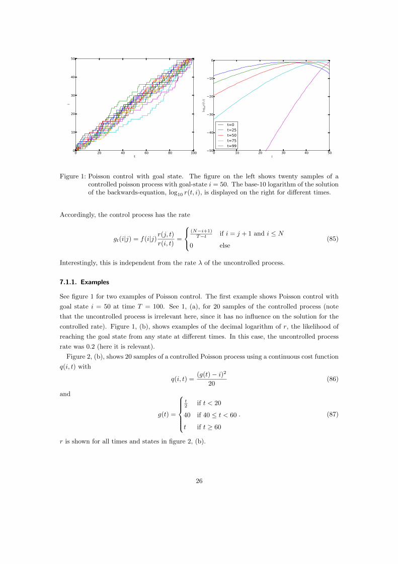
Figure 1: Poisson control with goal state. The figure on the left shows twenty samples of acontrolled poisson process with goal-state i = 50. The base-10 logarithm of the solutionof the backwards-equation, log10 r(t, i), is displayed on the right for different times.
Accordingly, the control process has the rate
gt(i|j) = f(i|j)r(j, t)r(i, t)
=
(N−i+1)T−t if i = j + 1 and i ≤ N
0 else(85)
Interestingly, this is independent from the rate λ of the uncontrolled process.
7.1.1. Examples
See figure 1 for two examples of Poisson control. The first example shows Poisson control with
goal state i = 50 at time T = 100. See 1, (a), for 20 samples of the controlled process (note
that the uncontrolled process is irrelevant here, since it has no influence on the solution for the
controlled rate). Figure 1, (b), shows examples of the decimal logarithm of r, the likelihood of
reaching the goal state from any state at different times. In this case, the uncontrolled process
rate was 0.2 (here it is relevant).
Figure 2, (b), shows 20 samples of a controlled Poisson process using a continuous cost function
q(i, t) with
q(i, t) =(g(t)− i)2
20(86)
and
g(t) =
t2 if t < 20
40 if 40 ≤ t < 60
t if t ≥ 60
. (87)
r is shown for all times and states in figure 2, (b).
26

0 20 40 60 80t
0
20
40
60
80i
0 50 100 150 200 250 300 350 400 450cost
0 10 20 30 40 50 60 70 80 90 100t
0
20
40
60
80
i
0.00 0.15 0.30 0.45 0.60 0.75 0.90r
Figure 2: Poisson control with time-dependent cost-function. The figure on the left shows twentysamples of a controlled poisson process with a time-dependent cost function as definedin section 7.1.1. The background of the graph is colored according to the values of thecost-function. The figure on the right depicts values of the backwards-solution, r(t, i),over time.
7.2. Single-Agent Control
Poisson process control is a special case (with very restricted dynamics) of single agent MJP-
control. More generally, the situation is this: Given D positions, we have a state-space S =
{0, . . . , D} and an uncontrolled process rate function f(i, j). Given an arbitrary state-dependent
cost function q(s, t) the control costs should be minimized. If D is a finite, not too large number,
this problem can be solved directly, using the results from Sections 6 and 4.5.
First of all, we note that the prior rate of the process (that is, the uncontrolled dynamics of
the system), can be characterized by a matrix C with Cij being the rate of the agent jumping to
position j if it is at position i, f(j|i) = Cij . Plus, we define a vector r with ri(t) = r(i, t). The
optimal action for this problem is given as the posterior MJP by equation 78. Its process rate
can be derived using the method from Section 4.5. The system’s backward equation becomes
∂
∂tri =
∑j 6=i
Cij(ri − rj) + qi(t)ri(t), (88)
with a cost-vector q(t). This is a system of D linear differential equations. For the special case
that there are only final costs at some time T , the solution is
r(t) = exp (C(T − t))> r(T ) (89)
(see appendix B for details), with boundary conditions
ri(T ) = exp(−qi(T )). (90)
27

Accordingly, we have for the posterior rate function gt(j|i) ..= Gij(t) = Cijrj(t)ri(t)
for i 6= j and
gt(i|i) ..= Gii = −∑j 6=i gt(j|i).
7.2.1. Weak Noise Approximation for Single-Agent Control
Deriving the posterior rate for the single-agent case involves the solution of a D-dimensional
system of linear differential equations. If D is large, this can become a problem.
With structured state-space and prior rate function, and a cost-function q(i, t) that is non-zero
only at some final time T , the solution can be simplified using the weak noise approximation
by [Ruttor et al., 2009] (see Section 9.1): As an example, we represent a state by a vector X ∈ Z2.
This can be interpreted as the position of the agent in a two dimensional grid, relative to some
origin. If the agent can only move to adjacent positions, uncontrolled rates can be specified as
f(
(a′
b′
),
(a
b
)) =
λleft(t,
ab
) if a′ − a = 1 and b′ = b
λright(t,
ab
) if a′ − a = −1 and b′ = b
λup(t,
ab
) if b′ − b = 1 and a′ = a
λdown(t,
ab
) if b′ − b = −1 and a′ = a
0 else.
(91)
Accordingly, the drift vector (equation 58, Section 5.1) becomes
f(X) =∑X′ 6=X
f(X ′|X)(X ′ −X) (92)
=
(λleft(t,X)− λright(t,X)
λup(t,X)− λdown(t,X)
), (93)
and the diffusion matrix (equation 59, Section 5.1)
D(X) =∑X′ 6=X
(X ′ −X)f(X ′|X)(X ′ −X)> (94)
=
(λleft(t,X) + λright(t,X) 0
0 λup(t,X) + λdown(t,X)
). (95)
Now,
r(X, t) ∝ exp
(−1
2(X − b(t))>B(t)−1(X − b(t))
)(96)
28

0 2 4 6 8 10t
0
10
20
30
40
i
0 2 4 6 8 10t
0
10
20
30
40
i
0 2 4 6 8 10t
0
10
20
30
40
i
0.075
0.050
0.025
0.000
0.025
0.050
0.075
0.100
Figure 3: Single-agent weak noise approximation in a one-dimensional state-space. On the left,the function r(i, t) computed according to the single-agent backwards-equation (equa-tion 88) is shown. The image in the center shows the corresponding weak noise ap-proximation rwn(i, t). The graph on the right depicts the difference r(i, t)− rwn(i, t).
with b(t) and B(t) evolving according to equations 60 and 64 (Section 9.1). If the rates are
independent from time and state, we get
b(t) = bT −
(λleft − λrightλup − λdown
)(T − t) (97)
B(t) = BT +
(λleft + λright 0
0 λup + λdown
)(T − t). (98)
where bT = e−q(T ) and qi(T ) ..= q(i, T ).
This result can be easily extended to N -dimensional state-spaces. In any case, computing the
posterior rate function involves solving systems of N linear differential equations, which simplifies
matters substantially, since usually N � D.
See Figure 3 for an example: Here, the solution to the backwards equation (equation 88) of
a single agent control problem on a one-dimensional state-space with 40 locations is shown on
the left, next to the weak noise approximation for the same task. The rightmost picture shows
the difference between the exact solution and the approximation. Note that the error is small
except at the edge of state space, which is due to the fact that the approximation presupposes
an infinite state-space.
7.2.2. Marginal Probability for Single-Agent Systems
Single-agent systems are trivially monomolecular – since there is only one agent, rates can never
depend on interactions between agents. For that reason, the expected state of the system can
be computed using equation 29 (Section 4.2). Agent’s locations at some time t are categorically
distributed and the marginal probability for an agent occupying location i is P (i, t) = E {X(t)i}.
29

7.2.3. Examples
As an example, let the task be to control an agent in such a way that it ends up at some
specified position sgoal at a given time T . The cost function encoding this problem could be
given as follows:
qi(t) =
∞ if t = T and i 6= sgoal
0 else. (99)
Consequently,
ri(T ) =
1 if i = sgoal
0 else. (100)
See figures 4 and 5 for simulation results: The one agent in this task starts at state 10 and is
supposed to reach state 35 at time T = 200. The uncontrolled process rate is set to a constant
value λ for adjacent states and 0, else. Figure 4, (a), shows one sample of a controlled agent
with λ = 1. For the sample in Figure 5, (a), λ = 10. Figures 4 and 5, (b), show expected values
over time for all states of the system for the controlled processes. Samples were acquired using
time-step-sampling (see Section 4.4) with appropriately small time steps.
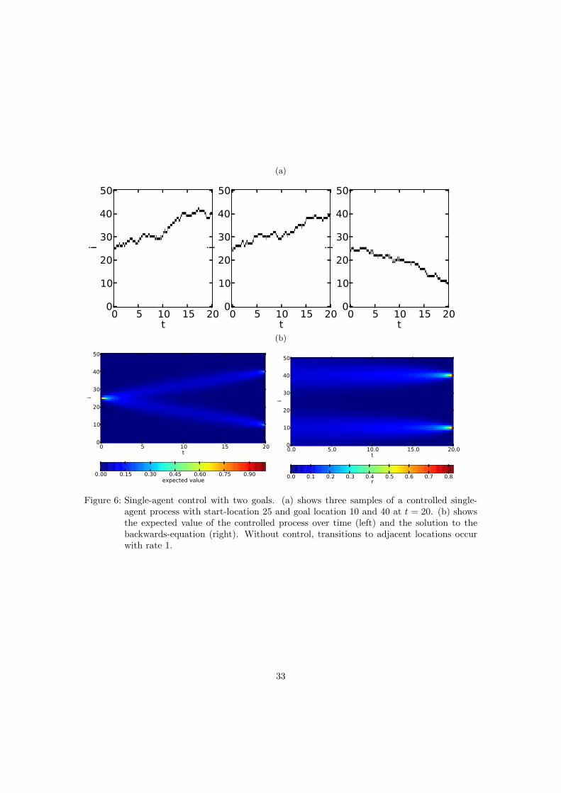
More complex cost functions are possible just as simple. See Figure 6 for a simulation with
two goal states that have equal costs.
Another example shows the effect of noise on control: in a setting with several goals, the
probability for the agent reaching a specific goal depends on the level of noise in the uncontrolled
dynamics. See Figure 7. Here, the agent starts at position 10 and may, by time T, move either
to position 40 at time T or return to position 10. With a low level of noise, the agent almost
always returns to position 10, since reaching position 40 would necessitate a high deviation from
the uncontrolled dynamics. In contrast, the agent ends up at position 40 more and more often
with increasing level of noise, because it may move close to that goal by chance.
A related interesting feature of stochastic control is symmetry breaking [Kappen, 2005]: if an
agent may choose between multiple goal states, control will be weak as long as the goal time is
sufficiently far in the future. The agent will first wander around without control, according to its
uncontrolled dynamics, and at the end steer to any goal that turned out close. This can be seen
in Figure 8. It shows the average deviation of the agents’ jump-rate from the uncontrolled rate
over time for different levels of noise in the uncontrolled dynamics for the task shown in Figure
6. The figure illustrates that if noise is high (red line), control happens mostly in the final stage
of the task, when the destination becomes clear and controlled movements will not be washed
out by future noise. If noise is low, though, (blue line) control is relatively uniform during the
whole task.
30

(a)
0 5 10 15 20t
0
10
20
30
40
50
i
0 5 10 15 20t
0
10
20
30
40
50
i
0 5 10 15 20t
0
10
20
30
40
50
i(b)
0 5 10 15 20t
0
10
20
30
40
50
i
0.00 0.15 0.30 0.45 0.60 0.75 0.90expected value
0 5 10 15 20t
0
10
20
30
40
50
i
0.0 0.1 0.2 0.3 0.4 0.5 0.6 0.7 0.8r
Figure 4: Single-agent control with low noise. (a) shows three samples of a controlled single-agentprocess with start-location 11 and goal location 35 at t = 20. (b) shows the expectedvalue of the controlled process over time (left) and the solution to the backwards-equation (right). Without control, transitions to adjacent locations occur with rate1.
31

(a)
0 5 10 15 20t
0
10
20
30
40
50
i
0 5 10 15 20t
0
10
20
30
40
50i
0 5 10 15 20t
0
10
20
30
40
50
i(b)
0 5 10 15 20t
0
10
20
30
40
50
i
0.00 0.15 0.30 0.45 0.60 0.75 0.90expected value
0 5 10 15 20t
0
10
20
30
40
50
i
0.00 0.04 0.08 0.12 0.16 0.20 0.24 0.28r
Figure 5: Single-agent control with high noise. (a) shows three samples of a controlled single-agent process with start-location 11 and goal location 35 at t = 20. (b) shows the ex-pected value of the controlled process over time (left) and the solution to the backwards-equation (right). Without control, transitions to adjacent locations occur with rate 10.
32
(a)
0 5 10 15 20t
0
10
20
30
40
50
i
0 5 10 15 20t
0
10
20
30
40
50i
0 5 10 15 20t
0
10
20
30
40
50
i(b)
0 5 10 15 20t
0
10
20
30
40
50
i
0.00 0.15 0.30 0.45 0.60 0.75 0.90expected value
0.0 5.0 10.0 15.0 20.0t
0
10
20
30
40
50
i
0.0 0.1 0.2 0.3 0.4 0.5 0.6 0.7 0.8r
Figure 6: Single-agent control with two goals. (a) shows three samples of a controlled single-agent process with start-location 25 and goal location 10 and 40 at t = 20. (b) showsthe expected value of the controlled process over time (left) and the solution to thebackwards-equation (right). Without control, transitions to adjacent locations occurwith rate 1.
33

0.0 5.0 10.0 15.0t
010203040
i
0.0 5.0 10.0 15.0t
010203040
i
0.0 5.0 10.0 15.0t
010203040
i
0 10 20 30 40 50λ
0.0
0.2
0.4
0.6
0.8
1.0
p
goal 1goal 2
Figure 7: The effect of noise. Three samples of a controlled single-agent process with two goal-locations are shown on the left. The uncontrolled rate for transition to neighboringlocation for the top sample is 0.1, for the other two samples it is 10. The graph on theright the probability of reaching the bottom goal (“goal 1”) or the top goal (“goal 2”),dependent on the transition rates of the uncontrolled process.
0.0 5.0 10.0 15.0 20.0t
0.0
0.5
1.0
1.5
2.0
2.5
3.0
3.5
4.0
4.5
mea
n co
ntro
l
λ=.1
λ=1
λ=10
Figure 8: Symmetry braking. Average control costs over time for single-agent goal-directed con-trol with uncontrolled transition rates λ = .1 (blue), λ = 1 (green) and λ = 10 (red).
34

8. Exact Multi-Agent Control
This section introduces exact methods for multi-agent control in Markov jump processes. Note
that in some cases, numerical solutions of differential equations may be necessary. “Exact” refers
to the remaining aspects of the methods.
8.1. Multi Agent Control with Linear Costs
Multi-agent control is simple if the state costs are linear functions of the state, that is q(X, t) =
q(t)>X, since in that case, the likelihood term in the corresponding inference problem factorizes
(i.e. exp(−q(t)>X
)=∏i exp (−qi(t)Xi)) and agents behave independently from each other.
Due to this, the posterior rate function can be computed by solving the problem for the single-
agent case if no new agents can enter the system5 (i.e. c0i = 0 for all i). For the posterior rate
function, we get
gt(X′|X) =
n∑i=1
n∑j=1
δX′,X−1i+1jGij(t)Xi, (101)
where Gij(t) is the single-agent posterior rate-matrix and 1i the ith column of the N×N identity
matrix.
One can also solve Multi-agent control with linear costs by computing
r(X, t) = a(t) exp(ln(r(t)>X
)(102)
with
dridt
= −∑k 6=0
cik(rk − 1)− qi(t)ri (103)
da
dt= −a
∑k 6=0
c0k(rk − 1). (104)
This result can be applied to systems with agents entering the system. See [Opper and Ruttor,
2010] for a derivation.
5Agents leaving the system can be modelled by introductin an absorbing state X0
35
0 4 9 14 19t
0
10
20
30
40
i
0 1 2 3 4 5 6 7 8 9 10 11 12 13 14 15 16 17 18 19 20 21 22 23 24 25 26number of agents
0 50 100 150t
0
10
20
30
40
i
10 8 6 4 2 0 2 4 6 8 10costs
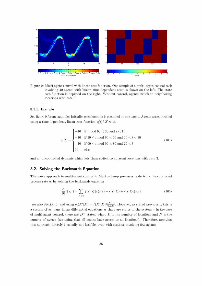
Figure 9: Multi-agent control with linear cost function. One sample of a multi-agent control taskinvolving 40 agents with linear, time-dependent costs is shown on the left. The statecost-function is depicted on the right. Without control, agents switch to neighboringlocations with rate 3.
8.1.1. Example
See figure 9 for an example: Initially, each location is occupied by one agent. Agents are controlled
using a time-dependent, linear cost-function q(t)>X with
qi(t) =
−10 if t mod 90 < 30 and i < 11
−10 if 30 ≤ t mod 90 < 60 and 10 < i < 30
−10 if 60 ≤ t mod 90 < 80 and 29 < i
10 else
(105)
and an uncontrolled dynamic which lets them switch to adjacent locations with rate 3.
8.2. Solving the Backwards Equation
The naıve approach to multi-agent control in Markov jump processes is deriving the controlled
process rate gt by solving the backwards equation
∂
∂tr(s, t) =
∑s′ 6=s
f(s′|s) (r(s, t)− r(s′, t)) + r(s, t)c(s, t) (106)
(see also Section 6) and using gt(X′|X) = f(X ′|X) r(X
′,t)r(X,t) . However, as stated previously, this is
a system of as many linear differential equations as there are states in the system – In the case
of multi-agent control, there are DN states, where D is the number of locations and N is the
number of agents (assuming that all agents have access to all locations). Therefore, applying
this approach directly is usually not feasible, even with systems involving few agents.
36

8.3. Forward Solution
A different approach exploits the fact that agents behave independently from each other without
control, which implies that in the absence of control, a multi-agent system is monomolecular.
Now, as stated in Section 4.5, r(X, t) = p(D>t|X(t) = X) – in the context of inference, the
solution of the backwards-equation equals the probability for future observations given the current
state of the system. Transferred to control, this means that r(X, t) = p(XT , T |X(t) = X), the
likelihood of reaching state XT at time T when starting at Xt. In a monomolecular system, one
can compute this probability directly by solving the (forward) Master equation, using the results
from [Jahnke and Huisinga, 2007, p. 11] (see Section 4.3) and derive the controlled process as
gt(X′|X) = f(X ′|X) r(X
′,t)r(X,t) .
For the marginal distribution p(·, T |Xt = X), we have6
p(·, T |Xt = X) =M(·, X(1)t ,p(1)(T − t)) ? · · · ?M(·, X(n)
t ,p(n)(T − t)) (107)
Where
dp(k)
dt= A(t)p(k) (108)
p(k)(0) = 1k. (109)
1k is the kth column of the D ×D identity matrix, D being the number of locations.
Here, we have one multinomial for each occupied location at the start-state X(t). This can
be used to compute r(X, t) = p(XT |X(t) = X) and thereby the process rate of the controlled
system.
The intuition is this: The location of an agent at time T is a categorically distributed random
variable with p(X(T ) = i|X(t) = k) = p(k)i (see Section 7.2.2). Each agent behaves independently
from all others, thus the locations at T of several agents starting at the same location are
multinomially distributed. The final state X(T ) is a sum over the states resulting from groups
of agents starting from the same location. Since all those groups are independent, the resulting
probability distribution will be a convolution of the individual probability distributions (the sum
over independent random variables is distributed according to the convolution over the individual
distributions).
In contrast to the naıve approach of solving the backwards equation directly, with required
the solution of a system of DN linear equations, this method requires solving at most D systems
of D equations (again, D being the number of locations and N the number of agents). Still,
the method can realistically only be applied to small systems because of the complexity of the
convolution.
Note that for computing the controlled rate gt, equation 108 needs to be solved at every
timestep for each occupied location, which is computationally demanding and can be an issue
6I neglect the case that new agents can enter the system.
37

when agents should be controlled in real-time. To circumvent this problem, one may precompute
parameter-vectors p for all times up to time T , the end of the trial, before starting it (when using
numerical solution methods for integrating the parameter vectors, this comes at the relatively
moderate cost of some additional memory). This reduces computation during actual control.
However, it needs to be done not only for those locations that are occupied at t = 0, but for all
locations that can possibly be reached.
8.4. Backward Solution
Using the same basic idea as before, it is also possible to compute an exact solution using the
single agent backwards solution for r(X, t): As stated in the previous section, an entry of a
parameter vector in the forward solution, p(k)i , can be interpreted as the single-agent marginal
probability p(X(T ) = i|X(t) = k) that the agent occupies location i at time T , given that it
started at location k at t. Now, this is exactly the solution r(i)k of the single-agent backwards
equation for a single-agent control task with goal state XT = i (see Section 7.2). Hence, one can
derive the marginal probabilities in the multi-agent case again as a convolution of multinomials
(equation 107), but using p(k)i = r
(i)k , where
dr(i)
dt= −C(t)r(i) (110)
r(i)(T ) = 1i, (111)
with C defined as in Section 7.2. As before, this allows one to compute r(X, t) = p(XT |X(t) = X)
and consequently the controlled process rate gt.
Computing the parameters this way has the advantage that, instead of solving the single-
agent backwards equation for every single location, one can specify a number of single agent
goals and compute the solution for these goals. The marginal probability distribution is then
over assignments of numbers of agents to single-agent goals instead of assignments of numbers of
agents to locations . This is beneficial from a computational point of view, since only as many
systems of equations need to be solved as there are goals. In addition, these goals need not
consist in reaching specific locations, they can be derived from any kind of state-dependent cost
function. In particular, this provides a way of doing a particular kind of multi-agent ergodic
control (see Section 10.2)
See Figure 10 for an example: Here, there are two single-agent goals to be fulfilled at time T ,
one consists in reaching location 0 and the other consists in ending up in the upper half of the
state space (locations 20 to 40). Both goals should be reached by exactly two agents.
Although the backwards method for computing parameters for the marginal probability is
arguably more efficient than the forward method, the complexity of the convolution remains.
38

0 5 10 15 20t
0
10
20
30
40
i
0 1 2 3 4number of agents
0 5 10 15 20t
0
10
20
30
40
i
0 1 2 3 4number of agents
Figure 10: Multi-agent goal-directed control with four agents. In the uncontrolled process, tran-sitions occur with rate 1.
9. Approximate Multi-Agent Control
One approach to render multi-agent MJP-control involving more than just a few agents feasible is
to exploit the equivalence of control to probabilistic inference and to apply approximate inference
techniques. In the following sections I present different methods based on this idea.
9.1. Weak Noise Approximation
One instance of an approximate inference method is the weak noise method as introduced in
Section 5.1. The methods can be used for control problems with a goal to reach a certain state
XT at time T and no further state dependent costs.
To repeat, the solution of the backwards equation r(X, t) is approximated by
r(X, t) ≈ η(t) exp
(−1
2(X − b(t))>B−1(t)(X − b(t))
), (112)
with b and B evolving according todb
dt= f(b), (113)
and
dB
dt= A(b(t))B(t)A(b(t))> −D(b(t)), (114)
39

with
f(X) =∑X′ 6=X
f(X ′|X)(X ′ −X) (115)
D(X) =∑X′ 6=X
(X ′ −X)f(X ′|X)(X ′ −X)> (116)
Aij(X) =∂fi∂xj
. (117)
For the control task to reach a goal XT at T , one gets boundary conditions b(T ) = XT and
B(T ) = 1ε with a small ε. Accordingly, the controlled rate of the process is approximated by
gt(X′|X) = f(X ′|X)
r(X ′, t)
r(X, t)(118)
≈ f(X ′|X)exp
(− 1
2 (X ′ − b(t))>)B−1(t)(X ′ − b(t)))
exp(− 1
2 (X − b(t))>B−1(t)(X − b(t))) (119)
= f(X ′|X) exp
(−1
2(X ′ −X)>B−1(t)(X ′ −X) + b(t)>B−1(t)(X ′ −X)
). (120)
An issue with the weak-noise approximation in the context of multi-agent control is the ap-
proximation of r by an unnormalized Gaussian: Since no location can be occupied by a negative
number of agents, this approximation is only valid if the mean b of the Gaussian is large (with re-
spect to the covariance matrix) in all dimensions. Problematically, in typical multi-agent control
scenarios, only few locations are occupied and many are empty. In particular, since b(T ) = XT ,
XT should be large in all dimensions. Even if that is the case, some entries of b may quckly
become small when developed according to equation 113. This can happen, for example, if tran-
sitions from some location i to a location k occur at a high rate, but not the other way round.
Given these considerations, one would expect the weak noise approximation to be appropriate
only for control of large numbers of agents.
A second problem with the weak noise approximation in the context of control is the assump-
tion that typical state vectors can be expected to be close to b(t). This assumption is needed
for the second expansion in the derivation of the weak noise approximation (equation 61, Section
5.1). While the assumption is justified in a probabilistic inference setting, this is not the case
for control: The assumption should hold for state vectors at all times, in particular for t = 0.
Hence, X(0) should be close to b(0). However, as X(0) is the starting state of the control task,
one should be able to choose it arbitrarily. See Figure 11 for an example illustrating the issue:
I performed 100 simulations of a control problem with a goal-state XT that has X(i)T = 100 for
all i and an initial state X(0) with X(0)(i) = 0 for all i except X(0)(5) = 1000. The rate of the
uncontrolled process is 1 for transitions to adjacent locations in either direction. Since there is no
drift in the system, b(t)i = 100 for all i and all t and the unnormalized Gaussian approximating
r is concentrated far from the boundary of state space at all times.
The overall average control costs using a controller based on the variational approximation
40

0.0 0.2 0.5 0.8 1.0t
02468
i
0.0 0.2 0.5 0.8 1.0t
02468
i
0 100 200 300 400 500 600 700 800 900 1000number of agents 0.0 0.2 0.4 0.6 0.8 1.0
t0
2000
4000
6000
8000
10000
aver
age
cont
rol c
ost
variational approximationweak noise approximation
Figure 11: Weak noise control. Left: Samples of a goal-directed control task using the variationalmethod (top) and the weak noise method (bottom). Right: Average control costs overtime using both methods.
(see next section) are 938. With the weak noise approximation, average control costs are larger
than 5.8 · 108. In contrast, in a control task with the same goal-state, but with a starting-state
that equals the goal-state, control costs using both methods are comparable.
9.2. Variational Approximation
One can approximate the posterior rate function of a multi-agent MJP using the variational
method7 by [Opper and Ruttor, 2010], outlined in Section 5.2. In a setting with goal-states, that
is with state-dependent costs that depend only on the success of reaching a certain state XT at
time T, the method can be directly adapted. The costs can be modeled as
1
2σ2||XT − L[X(T )]||2, (121)
the squared distance of the linearly transformed state of the system at time T from the goal
state XT8. σ2 can be seen as a parameter that specifies the penalty due to deviation from
the goal. Deviations will be tolerated more if σ2 is large. In that case the posterior rate
function gt will be more similar to the prior rate f than in the case of small σ2. We have
seen in Section 6 that the cost-function defined in equation 121 corresponds to a “likelihood”
p(XT |X(T )) = exp(− 1
2σ2 ||XT − L[X(T )]||2). This is exactly the measurement model [Opper
and Ruttor, 2010] use as a basis for their approximation (equation 67, Section 5.2) and the
method can be applied without further ado: As discussed in Section 5.2, the solution to the
7Note that this method only applies to monomolecular systems. In the case of multi-agent control it is applicabledue to the independence of agents without control.
8For simplicity, I will omit the linear transformation L in the following and assume it to be the identity function.
41

backwards equation r(X, t) can be approximated by
r(X, t) ≈ a(t) exp(ln r>X
), (122)
with r and a as defined in Section 5.2 and with a boundary condition r(T ) = exp(φ). φ maximizes
a variational lower bound to the free energy (equation 73, Section 5.2). It can be foud using
gradient ascent methods with the gradient
∇φf = −σ2φ+XT − E (L[X(t)]) . (123)
Here, the expectation is computed with respect to the current φ. Computing this expectation
can be expensive, as it involves solving a system of linear equations (equation 29, Section 4.2).
However, as is discussed in Section 8.1, in the case that no new agents can enter the system, the
multi-agent-control in the case of linear costs can be expressed as a combination of single-agent
solutions:
gt(S′|S) =
n∑i=1
n∑j=1
δS′,S−1i+1jGtijSi. (124)
If there are N goal locations that should be occupied by at least one agent with positive proba-
bility at time T one can express the controlled rate-matrix G as
Gtij =
f(j|i)∑N
k=1 wkr(t)(j)k∑N
k=1 wkr(t)(i)k
if i 6= j
−∑j 6=iG
tij else
, (125)
where r(t)(j)k are solution to the N single-agent control problems corresponding to each goal and
wk = eφk . We have
E [X(T )k|w, Xt] =
D∑i=0
X(i)t
wkr(t)(i)k
Z(i). (126)
Here,wkr(t)
(i)k
Z(i)..= P (k|i) can be interpreted as the likelihood that an agent occupying location i
at time t reaches goal k at T in the controlled process. X(i)t denotes the number of agents at
location i at t. Z(i) =∑Nl=0 wlr(t)
(i)l is a normalization term.
It is important to stress that the method cannot give a solution to the multi-agent control
problem directly: The posterior rate function in the approximation is determined by the “likeli-
hood”
r(X, t) ∝ exp(r(t)>X
)(127)
=
M∏i=1
exp (φ(t)iXi) (128)
42

(equation 69, Section 5.2). This likelihood factorizes. Consequently, the posterior factorizes if the
prior factorizes, which we assume9. This is a problem, since it implies that agents will behave
independently not only in the uncontrolled process, but also in the controlled process, which
contradicts the purpose of the whole procedure: in order to reach the goal state, agents can’t
act independently from each other since otherwise it is impossible to consistently get a specific
number of agents per location. See the next section for a further discussion of this issue.
Another direction one can take here is is to approximate the marginal distribution of X at
T by a Gaussian, wich gives a closed-form solution for φ. However, preliminary experiments
indicate that this is not appropriate for control. Plus, one can use the Gaussian approximation
directly for deriving controlled rates (see Section 9.5) without a further approximation using the
method presented in this section. See appendix C for details.
9.3. Expectation Control
One can gain a a further perspective on the above by approximating a solution to a non-linear
control problem using a linear cost-function by minimizing the divergence of the expected state
of a controlled process at time T from some goal state XT . Note that this does not solve the
problem of reaching XT in every individual trial.
In order to minimize the divergence of the expected state at T from the goal state XT , we
need to find a weight-vector w∗ with
w∗ = argminw
||E [X(T )|w, Xt]−XT ||2, (129)
where E [X(T )k|w, Xt] is defined as above (equation 126) The optimal weights can be found
using an iterative, EM-type procedure (see appendix D for a reformulation in the usual terms in
context of the EM-algorithm). In the E-step, the normalization Z(i) is computed. In the M-step,
the weights are optimized, using
wk =X
(k)T∑D
i=0X(i)t
r(t)(i)k
Z(i)
, (130)
which is found by differentiating the objective function
∂
∂wk
1
2||E [X(T )|w, Xt]−XT ||2 =
(wk
D∑i=0
X(i)t
r(t)(i)k
Z(i)−X(k)
T
)D∑i=0
X(i)t
r(t)(i)k
Z(i)(131)
!= 0. (132)
The result is guaranteed to improve in each step [Bishop, 2006] and one can stop iteration after
some error-criterion has been reached.
9This is equivalent to the observation that the posterior process will remain monomolecular if the prior processis monomolecular, made by [Opper and Ruttor, 2010, p. 5].
43

Returning to the discussion from the previous section, we see that if σ = 0, the gradient in
equation 123 can be rewritten in terms of w as
∂f
∂wk= E [X(T )k|w, Xt]
X(k)T∑D
i=1X(i)t
r(t)(i)k
Z
− wk
. (133)
The sign of the gradient does only depend onX
(k)T∑D
i=1X(i)t
r(t)(i)k
Z
−wk, therefore, using it in gradient-
ascent will lead to the same solution as using the update rule in equation 130. Hence, finding the
lower-bound of the free energy (equation 73, Section 5.2) and minimizing the distance between
the expected state of the process at T to some goal state are dual problems. Thus, a multi-agent
system that is controlled according to the method presented in the previous section would reach
the goal state in the expectation, but not in each individual trial.
The above is an interesting result in itself, since it provides an efficient method for computing
the expected evolution of a multi-agent system. Still, one can take a further step and derive
a control method. We note that if the covariance matrix of the marginal distribution at the
final time T under controlled dynamics is diagonal, that is, if the amounts of agents at different
locations are uncorrelated, a system controlled according to the approximation would reach the
goal state not only in the expectation, but in each individual trial. This is true because correlation
arises only if there are several ways to assign agents from start- to goal locations – if there exist
k and l with k 6= l such that P (k|i) > 0 and P (l|i) > 0 for some i with X(t)(i) > 0. If that is
not the case, there is only one option and the expectation becomes a deterministic solution. One
can expect correlation to be small if T − t is small with respect to the uncontrolled rates, since
in that case divergence between X(t) and X(T ) becomes expensive, which makes it likely that
a single agent is assigned to just one goal location. Hence, one can construct an approximately
exact controller by recomputing the above linear-cost approximation at every timepoint. As T−tbecomes small, the control will become more exact. In practice, one can monitor the expected
error ||E [X(T )|w, Xt]−XT ||2 and adapt the weights only whenever it exceeds some predefined
threshold. This adaptation should take only few iterations, because weights that minimize the
error can be expected to be close to previous weights. Simulations indicate that the method
works well, even if T − t is large (see Section 15).
9.4. Partial Evaluation of the Solution to the Forward Master Equation
We have seen in Sections 8.3 and 8.4 that one can get an exact solution for multi-agent control by
computing the solution to the forward Master equation, which is a convolutions of single-agent
solutions. However, each convolution involves a sum over too many terms for its computation
to be tractable for cases involving more than a handful of agents. One way to circumvent this
problem is to compute the solution to the Master equation only partially, leaving out most parts
of the sum and, doing this, approximate a solution.
Instead of expressing the probability r(X, t) = P (XT , T |X(t) = X) as a convolution of Multi-
44

nomials, one can express it as a sum over possible assignments from agents at time t to single-
agent goals r(X, t) =∑
a∈as r(a1)1 · · · r(an)
n , where as is the set of all possible assignments of agents
to goals – the probability of fulfilling a goal is the sum of probabilities of all possible ways to
fulfill it . In a situation where some agents are likely to reach only a subset of the goals under
the uncontrolled dynamics, some assignments of agents to goals are very unlikely and therefore
contribute very little to this sum. For that reason, it is reasonable to approximate r(X, t) by a
sum∑
a∈as∗ r(a1)1 · · · r(an)
n with as∗ = {a ∈ as | r(a1)1 · · · r(an)
n > ε}, the set containing assignments
which occur with a likelihood larger than some small ε.
Constructing as∗ directly is not helpful, since computing likelihoods for all assignments would
be as demanding as computing the whole sum directly. Instead, one can construct the set
heuristically – One method for doing this is to first assign agents to goals in such a way that those
agents get assigned first for which the drop in likelihood by getting assigned to a different would
be steepest 10 (See Algorithm 1 for the precise method) and then repeatedly create subsequent
assignments by switching assignments for pairs of agents (See Algorithm 2). This can be done
for all pairs11 of the most likely assignment that has been created so far.
However, this computation of assignments is computationally demanding and should not be
repeated each time r(X, t) needs to be evaluated (which is at every time step for the current
state of the system and all possible successor states, since gt(X′|X) = r(X′,t)
r(X,t) )). Instead, one can
compute assignments before control is started and subsequently adapt these as jumps occur. This
is based on the idea that relative likelihoods of assignments stay roughly constant. In practice,
it has proven useful to compute a number of assignments before the beginning of a control task,
then select the n most likely assignments and after each jump compute all possible resulting new
assignments, again selecting the n most likely for the continuation of the procedure.
In practice, one should take into account repetitions of assignments of agents that are at the
same location, by computing
r(X, t) =∑a∈as′
D∏i=1
Xi!
∏Dj=1(r
(j)1 )aj→1 · · · (r(j)
n )aj→n∏Nk=1
∏Dl=1 al→k!
(134)
instead of∑
a∈as∗ r(a1)1 · · · r(an)
n . Here, as′ is a set assignments of agents to goals with ai→k ∈ a
denoting the number of agents at position i that are assigned to goal k.
The number of likely assignments of agents to goals decreases as t approaches the final time T .
Thus, one can expect the approximation of r to be more accurate in late stages of control. See
Figure 12 for data illustrating this point. Here, a goal directed control task with 20 agents in one
dimension was performed 10 times. The graph on the left shows the average normalized difference
of two approximations of r(X, t) (rapprox) to its exact value (r) over time, i.e.r−rapprox
r . The
graph on the right shows average divergence of process rates gapprox using the approximation
from optimal process rates g, which is calculated as |1 − gapprox
g |. For the approximations, 1
10Assigning agents greedily would be another option, but has turned out to be less adequate.11Selecting only the best candidates for switching is computationally inefficient.
45

Algorithm 1: initial assignment
Data: the set G = {1 . . . N} of goal-indices; the set A = {1 . . . D} of agent-indicesResult: an assignment a ∈ DN from agents to goalswhile G not empty do
lowestRatio ←∞foreach i ∈ A do
bestGoal ← argmaxk∈G
r(i)k
best ← maxk∈G
r(i)k
secondBest ← maxk∈G\best
r(i)k
ratio ← secondBestbest
if ratio < lowestRatio thenlowestRatio ← rationextAgent ← inextGoal ← bestGoal
anextGoal ← nextAgentremove nextGoal from Gremove nextAgent from A
Algorithm 2: switching assignments
Data: the set as∗ of assignments for which flips have not been computedResult: as∗ with added assignments
a∗ ← argmaxa∈as∗
r(a1)1 . . . r
(an)n
for i ← 1 to n dofor j ← i + 1 to n do
a′ ← a∗
a′i ← a∗ja′j ← a∗iadd a′ to as∗
assignment and 10 assignments from agents to goals were used to estimate the solution of the
Master equation as explained above.
Note that differences in r are large in the beginning of the task and small at the end. Inter-
estingly, although the normalized difference of the approximation of r(X, t) to its exact value is
very large in the beginning of the task using an approximation based on one assignment from
agents to goals, this is not reflected in the divergence of process rates. An explanation may be
the following: In the beginning of the task, the likelihood of different assignments to goals is
relatively uniform across different assignments. For this reason, the approximation of r(X, t) is
rough if only few assignments are evaluated. However, for the same reason, differences between
r(X ′, t) and r(X, t) can be expected to be small for any X ′, both in the approximation and in
the exact solution and gt(X′|X) ≈ f(X ′|X).
46

0.0 0.2 0.4 0.6 0.8 1.0t
0.0
0.1
0.2
0.3
0.4
0.5
0.6
norm
aliz
ed d
iffer
ence
(r−r approx)/r
n=1
n=10
0.0 0.2 0.4 0.6 0.8 1.0t
0.00
0.01
0.02
0.03
0.04
0.05
0.06
0.07
dive
rgen
ce o
f rat
es |(
1−g approx/g
)|
n=1
n=10
Figure 12: Left: Average normalized difference of approximated likelihood rapprox to exact like-lihood r over time in a goal directed control task with 20 agents. Right: Averagedivergence of approximated controlled process rate to exact controlled process rates.Averages are over 10 trials.
9.5. Gaussian approximation
A further option to approximate the exact solution as given in Sections 8.3 and 8.4 is to use
a Gaussian approximation to the solution of the Master equation: A Multinomial distribution
M(·, N,p) is well approximated by a multivariate Normal distribution if N is large and p not
near the boundary of parameter space [Severini, 2005, p 378]. The sum of several independent
Gaussian random variables stays Gaussian [Severini, 2005, p 235], thus the marginal probability
of some state X at time t, being a sum of multiple independent Multinomials12, should be well
approximated by a Gaussian if the individual Multinomials satisfy the conditions for a Gaussian
approximation. Even if that is not the case, a Gaussian approximation of the marginal can still
be appropriate, since, due to the central limit theorem, the sum of several independent random
variables is closer to a Gaussian than the individual random variables.
The conditions for the appropriateness of a normal approximation of a Multinomial random
variable have two implications for its application in multi-agent control: First, there should be
many agents at each location (since that determines parameters N in the Multinomials) Second,
the likelihood r(k)i of an agent at location i reaching goal k should neither be close to one nor close
to zero for all agents and all goals (since, as shown in Section 8.4, r(k)i constitute the parameters p
in the Multinomials). The latter condition is most likely to be fulfilled if the uncontrolled process
rates are large in relation to T − t, the time remaining until the goal state is to be reached. In
any task this will eventually cease to be the case as T − t approaches 0. Still, the Gaussian
approximation may be an option for the early stages of control, where the methods presented in
Sections 9.2 and 9.4 have their weaknesses.
Mean and covariance matrix of the normal approximation are according to equations 40 and
12Independence follows from the monomolecularity of the uncontrolled process.
47

41, Section 4.3.
10. Ergodic Control
Ergodic control is control with a state dependent cost function q(X) that is independent of time.
Control should be maintained over indefinite time, thus the goal is not to minimize accumulated
costs, but to minimize a cost-rate.
10.1. Single-Agent Ergodic Control
With time-independent costs, the backward-equation for single-agent control becomes
dr
dt= −(C − Iq)r, (135)
where q is a cost-vector and C as defined in Section 7.2. For a final time T , this is solved by
r(T − t) =
D∑i=1
e−λi(T−t)v(i). (136)
where λi and v(i) are the eigenvalues and eigenvectors of −(C − Iq). Since, in ergodic control,
there is no final time T , we let T − t go to infinity. Doing this, |r| goes to 0. However, for
calculating ergodic controlled rates ge, we are only interested in ratios between ris. Hence,
ge(l|k) = f(l|k) limt→∞
rl(t)
rk(t)(137)
= f(l|k) limt→∞
(∑Di=1 e
−λitv(i))l(∑D
i=1 e−λitv(i)
)k
(138)
= f(l|k)v
(j)l
v(j)k
, (139)
with j = argmini
Re(λi). The last equality holds because in the limit the sum is dominated by
e−λjtv(j).
See Figure 13 for an example of single agent control and the largest eigenvector of the corre-
sponding backward-equation that is used for control.
10.2. Multi-Agent Ergodic Control
The result from the previous section can be transfered to the multi-agent case in a relatively
straight-forward way if costs can be constructed as combination of single agent-costs.
As we have seen, the likelihood r for single agents goes to zero in the limit of ergodic control.
Still, the controlled rates can be computed since they depend on the ratio between two rs that go
48
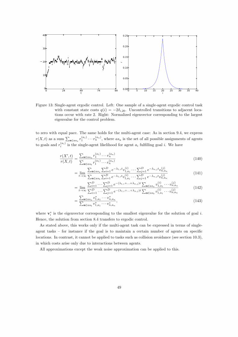
0 24 49 74 99t
0
10
20
30
40
i
0 5 10 15 20 25 30 35 40i
0.00
0.05
0.10
0.15
0.20
0.25
r
Figure 13: Single-agent ergodic control. Left: One sample of a single-agent ergodic control taskwith constant state costs q(i) = −2δi,20. Uncontrolled transitions to adjacent loca-tions occur with rate 2. Right: Normalized eigenvector corresponding to the largesteigenvalue for the control problem.
to zero with equal pace. The same holds for the multi-agent case: As in section 9.4, we express
r(X, t) as a sum∑
a∈asa r(a1)1 · · · r(an)
n , where asa is the set of all possible assignments of agents
to goals and r(ai)i is the single-agent likelihood for agent ai fulfilling goal i. We have
r(X ′, t)
r(X, t)=
∑a∈asa r
(a1)1 · · · r(an)
n∑a∈asb r
(a1)1 · · · r(an)
n
(140)
= limt→∞
∑a∈asa
∑Di=1 e
−λ1,itv(i)1,a1· · ·∑Dj=1 e
−λn,jtv(j)n,an∑
a∈asb∑Di=1 e
−λ1,itv(i)1,a1· · ·∑Dj=1 e
−λn,jtv(j)n,an
(141)
= limt→∞
∑Di=1 · · ·
∑Dj=1 e
−(λ1,i+...+λn,j)t∑
a∈asa v(i)1,a1· · · v(j)
n,an∑Di=1 · · ·
∑Dj=1 e
−(λ1,i+...+λn,j)t∑
a∈asb v(i)1,a1· · · v(j)
n,an
(142)
=
∑a∈asa v
∗1,a1 · · · v
∗n,an∑
a∈asb v∗1,a1· · · v∗n,an
, (143)
where v∗i is the eigenvector corresponding to the smallest eigenvalue for the solution of goal i.
Hence, the solution from section 8.4 transfers to ergodic control.
As stated above, this works only if the multi-agent task can be expressed in terms of single-
agent tasks – for instance if the goal is to maintain a certain number of agents on specific
locations. In contrast, it cannot be applied to tasks such as collision avoidance (see section 10.3),
in which costs arise only due to interactions between agents.
All approximations except the weak noise approximation can be applied to this.
49

0.0 25.0 50.0 75.0 100.00
10
20
30
40
0 4 9 13 18number of agents
Figure 14: Multi agent ergodic control. 18 agents with uncontrolled rates λ = 2 in either directionare controlled to minimize the cost rate with a state dependent cost-function as givenin section 10.2.1. All agents start at location 10.
10.2.1. Example
See figure 14 for an example of multi-agent ergodic control in one dimension. Single agent
state-dependent costs are defined as
q(i)j =
−2 if i = j
0 else(144)
with j ∈ {5, 15, 20, 25, 35}. q(i)20 is applied to ten agents, all other cost-functions are applied to
two agents, each. Uncontrolled process rates are λ = 2 for either direction.
10.3. Collision Avoidance
In collision avoidance, no two agents should ever occupy the same position. This can be expressed
with a state dependent cost function
q(X) =
∞ if maxiXi > 1
0 else(145)
This is a time-independent cost-function, thus the task is an instance of ergodic control. Un-
fortunately, one cannot easily express this as a combination of single-agent tasks, therefore the
results from the previous section do not apply directly.
Instead, we compute the likelihood of a collision given the current state, which can be expressed
50

as a product of likelihoods for pairwise collisions:
p(collision|Xt) =
N∏a=1
N∏b=a+1
p(collision(a, b)|Xt) (146)
One can compute r(a, b,Xt) ∝ p(collision(a, b)|Xt) as a ’single-agent’-solution in the product-
space S × S, with uncontrolled process rates
f((ja, jb)|(ia, ib)) =
f(ia|ja) if jb = ib and ja 6= ia
f(ib|jb) if ja = ia and jb 6= ib
f(ia|ja) + f(ib|jb) if jb = ib and ja = ia
0 else
. (147)
Using this, one can compute the solution for ergodic control with a cost-function
q(ia, ib) =
∞ if ia = ib
0 else(148)
with the method from section 10.1. The controlled rate for the process then becomes
g(X ′|X) = f(X ′|X)p(collision|X ′)p(collision|X)
(149)
= f(X ′|X)
∏Na=1
∏Nb=a+1 p(collision(a, b)|X ′)∏N
a=1
∏Nb=a+1 p(collision(a, b)|X)
(150)
= f(X ′|X)
∏Na=1
∏Nb=a+1 r(a, b,X
′)∏Na=1
∏Nb=a+1 r(a, b,X)
. (151)
Problematically, this requires the solution of the eigenvalue-problem for a D2 × D2 matrix.
However, once that solution is computed for a given state space, it can be used forever.
See Figure 15 for an example of collision avoidance in one dimension.
Figure 16 shows the solution of the ergodic control problem for collision avoidance in two-agent
product space.
51

0 8 17 26 34t
0
10
20
30
40
i
0 1number of agents
0 8 17 26 34t
0
10
20
30
40
i
0 1 2 3 4number of agents
Figure 15: Collision avoidance. The picture on the left shows a sample of a controlled multi-agent process with collision avoidance. For comparison, a sample of the uncontrolledprocess with the same initial state is shown on the right. Rates for transitions toneighboring locations are 1 in the uncontrolled case.
0 10 20 30 40i1
0
10
20
30
40
i2
0.000
0.005
0.010
0.015
0.020
0.025
0.030
0.035
0.040
0.045
r
Figure 16: Solution to the backwards equation for the ergodic collision-avoidance problem in thetwo-agent product space.
52

Part IV.
Simulations
In this part of the thesis, I present a series of simulations designed to evaluate the appropriateness
of the different approximate methods for multi-agent control presented in the thesis. The purpose
is to get answers to the following questions:
1. Do approximations work?
2. How does the performance depend on noise in the uncontrolled process?
3. How does the performance depend on the number of agents?
4. How does the performance depend on the number of dimensions?
5. How do different parameter settings influence the results?
6. How efficient are different approximations?
In the following, I outline the tasks used for simulations and reiterate some particularities of the
controllers used.
Note that the simulations are restricted to a subset of possible scenarios and care must be
taken in extrapolating insights gleaned from these scenarios to the general case.
11. Tasks
I measure the performance of approximate controllers using two general types of tasks: goal
directed control and ergodic control.
11.1. Goal directed control
In goal directed control, agents should reach a fixed state XT at time T . State dependent costs
are 0 if the goal state is reached and infinite if this is not the case. There are no further state
dependent costs. I perform simulations with different numbers of agents, different uncontrolled
process rates and in one-dimensional and two-dimensional state spaces. All simulations end at
T = 1. Transition rates are constant over time and equal for all possible transitions. See table 1
for specifications of simulations.
11.2. Ergodic control
In general, ergodic control is control with state-dependent costs which are independent of time.
In the particular kind of ergodic control tested here, there are N single-agent ergodic goals that
53

Simulation number of agents uncontrolled process rates number of dimensions1 5 5 12 5 20 13 5 100 14 20 5 15 20 20 16 100 1 17 100 1 18 5 5 29 5 20 2
Table 1: Simulations for goal-directed control.
should be fulfilled, each consisting in keeping an agent on some location i. Each single-agent
goal qi gives a reward (i.e. a negative cost) as long as it is fulfilled. The overall state-dependent
cost q(X) is then
q(X) =
∫ T
0
D∑i=1
min(Xi, ni)qidt, (152)
where −qi is the reward gained from keeping an agent at i and ni is the number of times that
reward is available (for instance, ni = 3 would imply that the reward at location i is maximized
at t if Xi(t) = 3.
Two simulations are performed. In both, agents move on a one-dimensional grid with 21
locations. State-dependent costs are according to equation 152 with
qi =
−2 if i ∈ {5, 10, 15}
0 else(153)
and
ni =
1 if i ∈ {5, 15}
3 if i = 10
0 else
. (154)
State transitions occur with rate 2 to adjacent locations in the first of the two simulations
(simulation 10) and with rate 10 in the second (simulation 11).
12. Controllers
Simulations are performed using all methods for multi-agent control discussed in the thesis, where
appropriate with multiple parameter-settings. In the following, I outline details related to the
different methods.
54

12.1. Exact Control
Exact control is performed according to the method presented in Section 8.4. Due to the com-
plexity of exact control it is only possible to perform in simple scenarios with few agents. Where
possible it serves as a point of reference for the evaluation of the performance of approximate
methods.
12.2. Variational Approximation
The variational approximation is performed as discussed in Section 9.3. Whenever the mean
squared error between the expected state at T and the goal state exceeds a predefined threshold
ε, the weights of the controller are updated according to the update rule defined in equation 130.
The approximation is tested using ε = .1, ε = 1−5 and ε = 1−10.
12.3. Partial Evaluation of the Solution to the Master Equation
A further control method tested here is based on the approximation of the solution to the Master
equation introduced in section 9.4. Before the control task is started, 1000 assignments of agents
to goals are computed. The n most likely assignments are kept and adapted to state changes
during control. The approximation is tested for n = 1, n = 10 and n = 100.
12.4. Weak Noise Approximation
The weak noise approximation is applied as explained in Section 9.1. The covariance matrix of the
unnormalized Gaussian approximating r is computed using a boundary condition B(t) = 0.1I,
where I is the identity matrix.
12.5. Gaussian Approximation
The Gaussian approximation is performed according to Section 9.5.
13. Sampling
State trajectories are sampled using Gillespie’s method (see Section 4.4). Note that samples
acquired using this method are only approximately correct, since rate-changes between jumps
are not accounted for. However, the error is small, since rates change slowly relative to the rate
of jumps.
55

14. Measure of Performance
Recall that the control-dependent costs are defined as the KL divergence between the controlled
process gt and the uncontrolled process f . The The KL-divergence between two MJPs is
KL(q||p) =
∫ T
0
dt∑X
q(X, t)∑X′ 6=X
(gt(X
′|X) lngt(X
′|X)
f(X ′|X)+ f(X ′|X)− gt(X ′|X)
). (155)
(equation 45, Section 4.5). One cannot evaluate this directly. However, it can be estimated as
KL(q||p) =
T/∆t∑i=0
∆t
n
∑X+
ti
∑X′ 6=X+
ti
(gt(X
′|X+ti ) ln
gt(X′|X+
ti )
f(X ′|X+ti )
+ f(X ′|X+ti )− gt(X ′|X+
ti )
). (156)
by sampling n trajectories X+. For the results presented here, n = 100 and ∆t = 0.1. In addition
to the overall control dependent costs, evolution of costs over time is shown.
15. Results
See Figures 17 to 28 for results of simulations. Error-bars correspond to the standard error of
the mean.
In the following, I shortly summarise the results.
15.1. Goal-Directed Control
Simulation 1 Goal directed control of five agents in a one dimensional grid with 41 locations.
Duration is 1, uncontrolled transitions occur with rate 5. See Figure 17 for results.
Control failed using the weak-noise approximation and the variational approximation using an
error threshold of ε = 0.1 (in both cases, the goal state was not reached). Average control costs
using the exact method were 20.14±0.58. Overall performance of all other methods was similar.
Average control costs using the Gaussian approximation were close to optimal (21.88± 0.69),
however, control is strong in the beginning of the trial and weak at the end of the trial. Using
all other methods, this is reversed.
Simulation 2 Goal directed control of five agents in a one dimensional grid with 41 locations.
Duration is 1, uncontrolled transitions occur with rate 20. See Figure 18 for results.
Average control costs using the exact method were 11.34 ± 0.33. Costs using the variational
method were close to optimal. The method based on the approximation of the solution to the
Master equation performed close to optimal for n = 10. Using n = 1 average control costs were
16.21± 0.47. Costs were sub-optimal in the beginning of the trial.
Costs for the Gaussian approximation were considerably higher than using the exact method,
28.1± 1.9.
56

The weak-noise method failed, giving average control costs that were several orders of magni-
tude higher than those of any other method.
Simulation 3 Goal directed control of five agents in a one dimensional grid with 41 locations.
Duration is 1, uncontrolled transitions occur with rate 100. See Figure 19 for results.
Control costs using the exact method were 7.34± 0.41. Results using the variational approxi-
mation were close to optimal. Using the approximation of the solution to the Master equation,
control costs were above optimal, 19.82± 1.94 for n = 1 and 12.23± 0.28 for n = 10. For these
methods, costs were sub-optimal in the beginning of the task. The Gaussian approximation
performed worse than optimal. Control costs were 20.47± 1.21.
The weak noise approximation failed, with control costs that were several orders of magnitude
higher than optimal.
Simulation 4 Goal directed control of 20 agents in a one dimensional grid with 41 locations.
Duration is 1, uncontrolled transitions occur with rate 5. See Figure 20 for results.
The exact method was not employed in this simulation since the task was too complex to make
an exact solution feasible.
Results were best using the variational approximation with an error criterion ε = 10−5 (average
control costs of 36.41± 0.94). The variational approximation with error criterion ε = 10−10 and
the approximation of the solution to the Master equation with n = 100 were close to that result
(39.75± 0.95 and 38.92± 0.88). The method based on the approximation of the solution to the
Master equation performed slightly worse for n = 1 and n = 10.
Average control costs using the weak noise approximation were far from optimal. Using the
method based on the variational approximation with an error criterion ε = 0.1 did not lead to
consistent fulfilment of the goal.
Simulation 5 Goal directed control of 20 agents in a one dimensional grid with 41 locations.
Duration is 1, uncontrolled transitions occur with rate 20. See Figure 21 for results.
Average control costs were lowest using the controller based on the variation approximation
(25.12± 0.56 for ε = 10−5, 25.32± 0.67 for ε = 10−10).
Control costs using the partial evaluation of the marginal were considerably higher and clearly
depended on the number n of assignments computed for the approximation (135.3±1.2 for n = 1,
87.35± 0.79 for n = 10 and 66.07± 0.69 for n = 100).
The Gaussian approximation resulted in average control costs that were much higher (215.70±139.0). Notably, the largest part of this exceeded cost comes from the last part of the task, shortly
before control was finished.
Average control costs using the weak-noise approximation were several orders of magnitude
higher than using any other method.
The goal was not fulfilled with the variational approximation and ε = 0.1.
57

Simulation 6 Goal directed control of 100 agents in a one dimensional grid with 10 locations.
Start-state and goal state are equal with 10 agents occupying each location. Duration is 1, un-
controlled transitions occur with rate 1. See Figure 22 for results.
Results were best using the variational method (average control costs of 15.01 ± 0.75 using
ε = 10−10 and 15.03 ± 0.84 using ε = 10−5). Average control costs using the method based on
the approximation of the solution to the Master equation were considerably higher (28.88± 0.72
for n = 1, 26.82 ± 0.53 for n = 10 and 27.38 ± 0.48 for n = 100). The Gaussian approximation
performed in a similar range, but with much higher variation (31.02± 13.06)
Again, the weak noise approximation led to control costs that were several orders of magnitude
higher than using all other methods. The variational approximation with ε = 0.1 did not lead
to a consistent fulfilment of the goal.
Simulation 7 Goal directed control of 100 agents in a one dimensional grid with 10 locations.
At t = 0, one location is occupied by 100 agents, all others are empty. In the goal state, all
locations are occupied by 10 agents. Duration is 1, uncontrolled transitions occur with rate 1.
See Figure 23 for results.
Average control costs were lowest using the variational approximation (107.64 ± 1.86 for ε =
10−5, 109.66 ± 1.55 for ε = 10−10). Using the approximation of the solution to the Master
equation, costs were slightly higher (114.69± 1.55 for n = 1 and 113.42± 1.8 for n = 10).
Although the overall costs using both these methods were similar, the evolution of costs over
time was different: Controllers based on the approximation of the solution to the Master equation
led to higher costs than those based on the variational approximation in the beginning of the
task and lower costs in the end.
Both the Gaussian approximation and the weak noise approximation led to average control
costs that were several orders of magnitude higher.
Control based on the variational approximation with ε = 0.1 did not fulfil the goal.
Simulation 8 Goal directed control of five agents in a two dimensional grid with 225 locations.
Duration is 1, uncontrolled transitions occur with rate 5. See Figure 24 for results.
Control using the exact method led to average control costs of 24.42±1.15. Results for control
using the variational approximation and using the approximation of the solution to the Master
equation were in a similar range.
The weak noise approximation and the Gaussian approximation did not work.
Simulation 9 Goal directed control of five agents in a two dimensional grid with 225 locations.
Duration is 1, uncontrolled transitions occur with rate 20. See Figure 25 for results.
Average control costs using the exact method were 17.6 ± 0.51. Results using both the vari-
ational approximation and the approximation of the solution to the Master equation were in a
similar range. One exception is the approximation of the Master equation with n = 1, where
costs were higher (22.37± 0.7), which is due to increased costs in the beginning of the trial.
58

The Gaussian approximation and the weak noise approximation did not work.
15.2. Ergodic Control
Simulation 10 Ergodic control with 5 agents. Duration of one trial is 100. Uncontrolled tran-
sitions occur with rate 2. See Figure 26 for results.
Overall costs using exact control were −2.78± 0.02.
Results using the approximation of the solution to the Master equation were in a similar range
with n = 10 (−2.8± 0.02). For n = 1, costs were slightly higher (−2.68± 0.02).
The costs using the variational approximation were close to optimal (−2.7± 0.02 for ε = 0.1,
−2.73 ± 0.017 for ε = 10−5 and −2.74 ± 0.02 for ε = 10−10). The control-dependent costs
under the variational approximation were lower than using exact control, the state-dependent
costs were higher (for the variational method with ε = 10−10, control-dependent costs were
0.93 ± 0.01, state-dependent costs −3.67 ± 0.02, using exact control, control-dependent costs
were 1.32± 0.01, state-dependent costs were −4.11± 0.05).
Average costs using the Gaussian approximation were sub-optimal (−2.27 ± 0.03). Notably,
the control-dependent costs were much higher than using any other method (3.7± 0.28) and the
state-dependent costs lower (−5.97± 0.02).
The weak noise method cannot be applied to ergodic control.
Simulation 11 Ergodic control with 5 agents. Duration of one trial is 100. Uncontrolled tran-
sitions to neighbouring locations occur with rate 10. See Figure 26 for results.
Overall costs using exact control were −1.55± 0.01.
Results for control using the variational approximation and using the approximation to the
solution of the Master equation with n = 10 were close to optimal. In all cases, average control-
dependent costs were low (0.1± 0.0001).
Average costs using control based on the approximation to the solution of the Master equation
with n = 1 were much higher (4.32± 0.03), which is mainly due to increased control-dependent
cost (5.96 ± 0.02), the state-dependent cost was comparable to that obtained using the other
methods.
Average costs for the Gaussian approximation were high (3.35± 0.003).
15.3. Noise
Simulation 12 Goal directed control with 5 agents in a two-dimensional grid with 41 locations
and varying transition rates in the uncontrolled process. Duration of one trial is 1. See Figure
28.
Average control costs relative to the costs obtained using the exact method increased with
the uncontrolled process rates in the method based on the approximation of the solution to the
Master equation.
59

0.0 0.2 0.5 0.8 1.0t
0
10
20
30
40i
0 1 2 3number of agents
0.0 0.1 0.2 0.3 0.4 0.5 0.6 0.7 0.8 0.9t
0
10
20
30
40
50
60
70
80
90
aver
age
cont
rol c
osts
variational control, εmax=10−5
variational control, εmax=10−10
approximation of the ME, n=1
approximation of the ME, n=10
Gaussian approximationexact control
1 2 3 4 5 6controller
0
5
10
15
20
25
aver
age
cont
rol c
osts
1 2 3 4 5 6controller
0
20
40
60
80
100
time
(s)
Figure 17: Simulation 1. Goal-directed control of five agents on a one-dimensional grid withuncontrolled transition rate λ = 5. Top left: One sample of the control task. Topright: Average control costs over time. Bottom left: Overall average control costs.Bottom right: Computation time. Controllers are: 1: Variational control, ε = 10−5.2: Variational control, ε = 10−10. 3: Approximation of the solution to the Masterequation, n = 1. 4: Approximation of the solution to the Master equation, n = 10.5: Gaussian approximation. 6: Exact control.
Using the Gaussian approximation, average control costs were higher than with the exact
method, but, relative to the costs obtained with the exact method, constant with respect to the
uncontrolled process rates.
For all other methods, average control costs were close to those of the exact solution.
60

0.0 0.2 0.5 0.8 1.0t
0
10
20
30
40
i
0 1 2 3number of agents
0.0 0.1 0.2 0.3 0.4 0.5 0.6 0.7 0.8 0.9t
0
20
40
60
80
100
120
aver
age
cont
rol c
osts
variational control, εmax=10−5
variational control, εmax=10−10
approximation of the ME, n=1
approximation of the ME, n=10
Gaussian approximationexact control
1 2 3 4 5 6controller
0
5
10
15
20
25
30
35
aver
age
cont
rol c
osts
1 2 3 4 5 6controller
0
50
100
150
200
250
300
time
(s)
Figure 18: Simulation 2. Goal-directed control of five agents on a one-dimensional grid withuncontrolled transition rate λ = 20. Top left: One sample of the control task. Topright: Average control costs over time. Bottom left: Overall average control costs.Bottom right: Computation time. Controllers are: 1: Variational control, ε = 10−5.2: Variational control, ε = 10−10. 3: Approximation of the solution to the Masterequation, n = 1. 4: Approximation of the solution to the Master equation, n = 10.5: Gaussian approximation. 6: Exact control.
61

0.0 0.2 0.5 0.8 1.0t
0
10
20
30
40
i
0 1 2 3number of agents
0.0 0.1 0.2 0.3 0.4 0.5 0.6 0.7 0.8 0.9t
0
20
40
60
80
100
120
140
160
aver
age
cont
rol c
osts
variational control, εmax=10−5
variational control, εmax=10−10
approximation of the ME, n=1
approximation of the ME, n=10
Gaussian approximationexact control
1 2 3 4 5 6controller
0
10
20
30
40
50
60
aver
age
cont
rol c
osts
1 2 3 4 5 6controller
0
100
200
300
400
500
600
time
(s)
Figure 19: Simulation 3. Goal-directed control of five agents on a one-dimensional grid withuncontrolled transition rate λ = 100. Top left: One sample of the control task. Topright: Average control costs over time. Bottom left: Overall average control costs.Bottom right: Computation time. Controllers are: 1: Variational control, ε = 10−5.2: Variational control, ε = 10−10. 3: Approximation of the solution to the Masterequation, n = 1. 4: Approximation of the solution to the Master equation, n = 10.5: Gaussian approximation. 6: Exact control.
62

0.0 0.2 0.5 0.8 1.0t
0
10
20
30
40
i
0 1 2 3 4number of agents 0.0 0.1 0.2 0.3 0.4 0.5 0.6 0.7 0.8 0.9
t0
200
400
600
800
1000
1200
1400
aver
age
cont
rol c
osts
variational control, εmax=10−5
variational control, εmax=10−10
approximation of the ME, n=1
approximation of the ME, n=10
approximation of the ME, n=100
Gaussian approximation
1 2 3 4 5 6controller
0
50
100
150
200
aver
age
cont
rol c
osts
1 2 3 4 5 6controller
0
100
200
300
400
500
600
time
(s)
Figure 20: Simulation 4. Goal-directed control of 20 agents on a one-dimensional grid withuncontrolled transition rate λ = 5. Top left: One sample of the control task. Topright: Average control costs over time. Bottom left: Overall average control costs.Bottom right: Computation time. Controllers are: 1: Variational control, ε = 10−5.2: Variational control, ε = 10−10. 3: Approximation of the solution to the Masterequation, n = 1. 4: Approximation of the solution to the Master equation, n = 10.5: Approximation of the solution to the Master equation, n = 100. 6: Gaussianapproximation.
63

0.0 0.2 0.5 0.8 1.0t
0
10
20
30
40
i
0 1 2 3 4number of agents 0.0 0.1 0.2 0.3 0.4 0.5 0.6 0.7 0.8 0.9
t0
500
1000
1500
2000
2500
aver
age
cont
rol c
osts
variational control, εmax=10−5
variational control, εmax=10−10
approximation of the ME, n=1
approximation of the ME, n=10
approximation of the ME, n=100
Gaussian approximation
1 2 3 4 5 6controller
0
50
100
150
200
250
300
350
400
aver
age
cont
rol c
osts
1 2 3 4 5 6controller
0
500
1000
1500
2000
2500
time
(s)
Figure 21: Simulation 5. Goal-directed control of 20 agents on a one-dimensional grid withuncontrolled transition rate λ = 20. Top left: One sample of the control task. Topright: Average control costs over time. Bottom left: Overall average control costs.Bottom right: Computation time. Controllers are: 1: Variational control, ε = 10−5.2: Variational control, ε = 10−10. 3: Approximation of the solution to the Masterequation, n = 1. 4: Approximation of the solution to the Master equation, n = 10.5: Approximation of the solution to the Master equation, n = 100. 6: Gaussianapproximation.
64

0.0 0.2 0.5 0.8 1.0t
0
2
4
6
8
i
7 11 15number of agents 0.0 0.1 0.2 0.3 0.4 0.5 0.6 0.7 0.8 0.9
t0
50
100
150
200
250
300
aver
age
cont
rol c
osts
variational control, εmax=10−5
variational control, εmax=10−10
approximation of the ME, n=1
approximation of the ME, n=10
approximation of the ME, n=100
Gaussian approximation
1 2 3 4 5 6controller
0
5
10
15
20
25
30
35
40
45
aver
age
cont
rol c
osts
1 2 3 4 5 6controller
0
200
400
600
800
1000
1200
1400
1600
1800
time
(s)
Figure 22: Simulation 6. Goal-directed control of 100 agents on a one-dimensional grid withuncontrolled transition rate λ = 1. Top left: One sample of the control task. Topright: Average control costs over time. Bottom left: Overall average control costs.Bottom right: Computation time. Controllers are: 1: Variational control, ε = 10−5.2: Variational control, ε = 10−10. 3: Approximation of the solution to the Masterequation, n = 1. 4: Approximation of the solution to the Master equation, n = 10. 5:Approximation of the solution to the Master equation, 6: Gaussian approximation.
65

0.0 0.2 0.5 0.8 1.0t
0
2
4
6
8
i
0 25 50 75 100number of agents 0.0 0.1 0.2 0.3 0.4 0.5 0.6 0.7 0.8 0.9
t0
50
100
150
200
250
300
aver
age
cont
rol c
osts
variational control, εmax=10−5
variational control, εmax=10−10
approximation of the ME, n=1
approximation of the ME, n=10
approximation of the ME, n=100
1 2 3 4 5controller
0
20
40
60
80
100
120
aver
age
cont
rol c
osts
1 2 3 4controller
0
50
100
150
200
250
300
time
(s)
Figure 23: Simulation 7. Goal-directed control of 100 agents on a one-dimensional grid withuncontrolled transition rate λ = 1. Top left: One sample of the control task. Topright: Average control costs over time. Bottom left: Overall average control costs.Bottom right: Computation time. Controllers are: 1: Variational control, ε = 10−5.2: Variational control, ε = 10−10. 3: Approximation of the solution to the Masterequation, n = 1. 4: Approximation of the solution to the Master equation, n = 10.5: Approximation of the solution to the Master equation, n = 100.
66

0 2 4 6 8 10 12 1402468
101214
0 2 4 6 8 10 12 1402468
101214
0 1 2number of agents 0.0 0.1 0.2 0.3 0.4 0.5 0.6 0.7 0.8 0.9
t0
20
40
60
80
100
mea
n co
ntro
l cos
t
variational control, εmax=10−5
variational control, εmax=10−10
approximation of the ME, n=1
approximation of the ME, n=10
exact control
1 2 3 4 5controller
0
5
10
15
20
25
30
mea
n co
ntro
l cos
t
1 2 3 4 5controller
0
50
100
150
200
time
(s)
Figure 24: Simulation 8. Goal-directed control of five agents on a two-dimensional grid withuncontrolled transition rate λ = 5. Top left: Start- and goal-state of the task. Topright: Average control costs over time. Bottom left: Overall average control costs.Bottom right: Computation time. Controllers are: 1: Variational control, ε = 10−5.2: Variational control, ε = 10−10. 3: Approximation of the solution to the Masterequation, n = 1. 4: Approximation of the solution to the Master equation, n = 10.5: Exact control.
67

0 2 4 6 8 10 12 1402468
101214
0 2 4 6 8 10 12 1402468
101214
0 1 2number of agents 0.0 0.1 0.2 0.3 0.4 0.5 0.6 0.7 0.8 0.9
t0
20
40
60
80
100
120
140
aver
age
cont
rol c
osts
variational control, εmax=10−1
variational control, εmax=10−10
variational control, εmax=10−10
approximation of the ME, n=1
approximation of the ME, n=10
exact control
1 2 3 4 5 6controller
0
5
10
15
20
25
aver
age
cont
rol c
osts
1 2 3 4 5 6controller
0
200
400
600
800
1000
1200
1400
time
(s)
Figure 25: Simulation 9. Goal-directed control of five agents on a two-dimensional grid withuncontrolled transition rate λ = 20. Top left: Start- and goal-state of the task. Topright: Average control costs over time. Bottom left: Overall average control costs.Bottom right: Computation time. Controllers are: 1: Variational control, ε = 10−1.2: Variational control, ε = 10−5. 3: Variational control, ε = 10−10. 4: Approximationof the solution to the Master equation, n = 1. 5: Approximation of the solution tothe Master equation, n = 10. 6: Exact control.
68

0.0 25.0 50.0 75.0 100.0t
0
5
10
15
20
i
0 1 2 3 4number of agents
1 2 3 4 5 6 7controller
6
4
2
0
2
4
aver
age
cost
s
control costsstate-dependent costs
1 2 3 4 5 6 7controller
3.0
2.5
2.0
1.5
1.0
0.5
0.0
aver
age
cost
s
1 2 3 4 5 6 7controller
0
50
100
150
200
250
time
(s)
Figure 26: Simulation 10. Ergodic control of five agents on a one-dimensional grid with un-controlled transition rate λ = 5. Top left: One sample of the control task. Top right:Average control costs and state dependent costs. Bottom left: Overall average con-trol costs. Bottom right: Computation time. Controllers are: 1: Variational control,ε = 10−1. 2: Variational control, ε = 10−5. 3: Variational control, ε = 10−10. 4:Approximation of the solution to the Master equation, n = 1. 5: Approximation ofthe solution to the Master equation, n = 10. 6: Gaussian approximation. 7: Exactcontrol.
69

0.0 25.0 50.0 75.0 100.0t
0
5
10
15
20
i
0 1 2 3 4number of agents
1 2 3 4 5 6 7controller
4
2
0
2
4
6
8
aver
age
cost
s
control costsstate-dependent costs
1 2 3 4 5 6 7controller
2
1
0
1
2
3
4
5
aver
age
cost
s
1 2 3 4 5 6 7controller
0
200
400
600
800
1000
1200
1400
time
(s)
Figure 27: Simulation 11. Ergodic control of five agents on a one-dimensional grid with uncon-trolled transition rate λ = 20. Top left: One sample of the control task. Top right:Average control costs and state-dependent costs. Bottom left: Overall average con-trol costs. Bottom right: Computation time. Controllers are: 1: Variational control,ε = 10−1. 2: Variational control, ε = 10−5. 3: Variational control, ε = 10−10. 4:Approximation of the solution to the Master equation, n = 1. 5: Approximation ofthe solution to the Master equation, n = 10. 6: Gaussian approximation. 7: Exactcontrol.
70

10 20 30 40 50 60 70 80 90level of noise
5
10
15
20
25
30
35
40
45
50
aver
age
cont
rol c
osts
variational control, εmax=10−10
approximation of the ME, n=1
approximation of the ME, n=10
Gaussian approximationexact control
Figure 28: Simulation 12 The effect of noise. Average control costs over 10 samples dependingon transition rates in the uncontrolled system in a goal directed control task with 5agents. Duration of the task was 1.
71

Part V.
Discussion & Conclusion
16. Discussion
The objective of this work was to develop efficient methods for multi-agent control in Markov
jump processes building on the LSMDP framework and using approximate inference techniques.
Exact optimal control is feasible for single-agent systems and multi-agent systems with state-
dependent cost-functions that depend linearly on the state vector of the controlled system. In
general, exact optimal control for multi-agent systems is intractable and approximate methods
are needed.
This thesis introduces approximate methods for two general types of tasks, goal directed
multi-agent control and ergodic multi-agent control. These methods include a weak-noise ap-
proximation, a variational approximation, a partial evaluation of the analytical solution to the
forward Master equation and a Gaussian approximation.
Simulations indicate that both the variational approximation and the partial evaluation of the
analytical solution to the Master equation are, with some restrictions, appropriate methods for
approximate control of multi-agent systems.
The controller based on a variational approximation performed close to optimal in simulations
where optimal results are available (Simulations 1, 2, 3, 8, 9, 10 and 11). Where this is not the
case its results are consistently among the best. The minimum error criterion in the method
seems to have only a small effect both on performance of the method and on computation time.
This goes with the restriction that, evidently, if the error criterion is too high, fulfillment of the
goal cannot be guaranteed. Interestingly control was good not only in the late stages of the
tasks (when T − t is small), which was expected (as discussed in Section 9.3) but over the whole
duration.
The method based on the partial evaluation of the solution to the Master-equation is par-
ticularly successful in the case of low noise in the uncontrolled process and few agents (as in
Simulations 1 and 8). If noise is high, the control costs are suboptimal in the early stages of
control if the approximation is coarse (Simulations 2, 3 and 8, in particular Simulation 12). This
is probably due to the fact that the approximation is based on selecting a subset of assignments
from agents to goals. If noise is low, this selection is more likely to reflect the final state of
the system than if noise is high. This effect relates to the phenomenon of symmetry braking
(cf. [Kappen, 2005]) – in stochastic control with high noise most control takes place in the last
stages of a trial, since early control is less effective because of the noise that perturbs the state
in the time remaining until the end of the task.
The weak-noise approximation failed to give satisfying solutions to control problems in all
simulations. The reason for this may be that in all cases the number of agents were relatively
72

low (see Section 9.1 for further discussion).
Performance of the Gaussian approximation of the solution to the Master equation was far
from optimal in all simulations. Again, this may be due to the low number of agents used in
the simulations. However, in Simulation 6, where the number of agents was comparably high
(100), the method performed poorly only in the last stage of the task. This is expected, since the
assumptions for a Gaussian approximation are violated for small T − t, as discussed in Section
9.5. Thus the method may still be appropriate in some restricted cases.
In all methods, the computation time depends on the transition rate in the uncontrolled
process, the number of agents and the dimensionality of state-space. The reasons are twofold:
First, since sampling is based on Gillespie’s method, the number of times the controlled process
rate function is evaluated depends on the number of jumps. That, in turn, increases both with
the number of agents and with the uncontrolled process rate. Second, the number of possible
successors for a given state depends on the number of agents and the dimensionality of state-
space. Since the controlled process rate function needs to be evaluated for all possible successor
states, computation time rises.
Note that except for the weak noise approximation, the number of states in the system influ-
ences computation time only through the computation of single-agent solutions, which is done
before a control trial starts. Computing single-agent solutions can become a problem if the num-
ber of states is large. In some situations it may be appropriate to use approximate methods such
as the weak-noise approximation for single-agents introduced in Section 7.2.1.
In the case of the variational approximation, necessary computation increases with the number
of goal locations due to the increased number of parameters in the optimization. Still, compu-
tation time was relatively low in all simulations. The dependence of computation time on the
value of the error criterion ε was negligible. The reason for this may be that the weights are
not recomputed each time the error threshold is exceeded, they are merely adapted. Since that
adaptation starts with an error slightly over the error criterion ε, irrespective of its value, the
time until the error falls again below that threshold should only weakly depend on it.
Computation time using the controller based on the partial evaluation of the solution to the
Master equation depends heavily on the number of computed assignments. It can be very fast
if the approximation is based on few assignments from agents to goals (using n = 1, the method
was fastest almost all simulations) and relatively slow if many assignments are computed.
17. Challenges
This thesis was the first attempt on tackling the problem of multi-agent control in Markov
jump processes using methods borrowed from approximate inference. Although first results are
promising, many challenges remain.
The methods developed for multi-agent control are only appropriate for goal-directed control
and ergodic control (if costs-function are non-linear). In particular, they cannot be applied to
cost-functions that are time dependent and yield costs that are non-zero for more than one time
73

point. While it seems reasonable to extend the methods presented here to cost-functions that
are non-zero at multiple isolated time-points, a transfer to tasks with continuous cost-functions
seems difficult. In these cases, methods based on sampling of state trajectories may be more
appropriate.
In the case of ergodic control, the presented methods work only on the special cases in which
state-dependent costs can be conceived as a combination of single-agent ergodic state-dependent
costs or for collision avoidance. One should further investigate ergodic control on a more general
level.
A further future direction of research concerns the application of the presented methods to
real-world scenarios. A topic that has not been touched in this thesis, but which would be
important for applications is the translation of transition probabilities to action commands.
The simulations performed in the thesis were all on structured, grid-like, state-spaces in which
transitions can only take place between adjacent locations. However, all methods introduced in
this thesis (with the exception of the weak-noise approximation) can be applied to processes with
arbitrary transition functions. One should investigate how the methods work in such contexts,
especially since this is an central feature that distinguishes control on Markov jump processes
from control in continuous space, such as path integral control.
Throughout the thesis, I assume that uncontrolled process rates are known. In real-world
scenarios this is likely not to be the case and one should investigate efficient methods for approx-
imating the uncontrolled process rates from data.
18. Further Approaches
I investigated the possibility of multi-agent control using two further methods that are not dis-
cussed in the thesis. The first is based on a computation of the analytical solution to the forward
Master-equation using the Fourier transform, the second is an approximation of the solution
to the Master equation using Belief propagation. Both methods appear to be computationally
too demanding to accomplish the task in a time appropriate for control applications. However,
investigation in these directions was only preliminary.
19. Conclusion
The purpose of this thesis was to develop efficient methods for multi-agent control on Markov
jump processes building on the framework of linearly solvable Markov decision processes and ap-
proximate inference. Five different methods were presented, discussed and tested in simulations.
Notably, a method based on an approximation using a variational lower bound to the free
energy of the controlled process performed well in all tested scenarios.
The thesis opens a promising new direction for research in multi-agent control which should
be further pursued.
74

20. Acknowledgements
I thank Prof. Manfred Opper and Dr. Andreas Ruttor for their supervision and patient support
during the preparation of the thesis. I also thank Duncan Blythe for proofreading.
75

A. MJP Inference with Arbitrary Cost Function
With an arbitrary cost function c(s, t), the KL(q||ppost) becomes
KL(q||ppost) = Ex∼q(·)
{ln
q(x)
ppost(x)
}(157)
= Ex∼q(·)
lnq(x)
1Z pprior(s) exp
(−∫ T
0c(x(t), t)dt
) (158)
= lnZ + KL(q||pprior) + Ex∼q(·)
{∫ T
0
c(x, t)dt
}(159)
The partial derivative of this with respect to q(s, t) is
δ
δq(s, t)KL(q||ppost) =
δ
δq(s, t)KL(q||pprior) + c(s, t) (160)
Hence the derivative of the Lagrangian becomes
δL
δq(s, t)=∑s′ 6=s
(gt(s
′|s) lngt(s
′|s)f(s′|s)
− gt(s′|s) + f(s′|s))
(161)
+∂
∂tλ(s, T ) +
∑s′
gt(s′|s) (λ(s′, t)− λ(s, t)) (162)
+ c(s, t) (163)
= 0 (164)
=∑s′ 6=s
(r(s′, t)
r(s, t)f(s′|s) ln
r(s′, t)
r(s, t)− r(s′, t)
r(s, t)f(s′|s) + f(s′|s)
)(165)
− ∂
∂tln r(s, t) (166)
−∑s′
r(s′, t)
r(s, t)f(s′|s) ln
r(s′, t)
r(s, t)(167)
+ c(s, t) (168)
=∑s′ 6=s
f(s′|s)(
1− r(s′, t)
r(s, t)
)− ∂
∂tln r(s, t) + c(s, t) (169)
(170)
This yields for the differential equation
∂
∂tr(s, t) =
∑s′ 6=s
f(s′|s) (r(s, t)− r(s′, t)) + c(s, t)r(s, t) (171)
76

B. Single Agent Control
∂
∂tpi =
∑j 6=i
Cij(pi − pj) (172)
= pi∑j 6=i
Cij −∑j 6=i
Cijpj (173)
= −piCii −∑j 6=i
Cijpj (174)
= −∑j
Cijpj (175)
→ d
dtp = −Cp (176)
This is solved by
p(t) = exp(C(T − t))>p(T ). (177)
C. Variational Approximation with Gaussian Marginal
We approximate the marginal distribution P (X,T ) of state vectors X at time T by a Gaussian
with mean µ and covariance Σ (from 41, section 4.3). φ>X(T ) will then be normally distributed
with mean φ>µ and variance φ>Σφ. Given that assumption, exp(φ>XT
)is distributed according
to a log-normal distribution and we have lnE[exp
(φ>X(T )
)]= φ>µ + 1
2φ>Σφ. The term to
maximize is then
f = −σ2
2||φ||2 + φ>XT − φ>µ−
1
2φ>Σφ>, (178)
by differentiating, one gets
∂f
∂φi= −σ2φi +XTi − µi −
∑j
φj .Σij (179)
Setting this to 0, the solution for φ turns out to be
φ = (σ2I + Σ)−1(XT − µ). (180)
D. EM-Formulation of Expectation Control
We introduce a likelihood function
p(Xt,Z|w) ∝ exp
(−||w
D∑i=1
X(i)t
r(t)(i)
Z(i)−XT ||2
). (181)
77

The E-step consists in finding the likelihood p(Z|Xt,w), which we define as
p(Z|Xt,w) ..=
D∏i=1
δ
(Z(i) −
N∑l=1
wlr(t)(i)l
). (182)
The goal of the M-step is to find parameters w that maximize
Q(w,wold) =∑Z
p(Z|Xt,w(old)) ln p(Xt,Z|w) (183)
= −||wD∑i=1
X(i)t
r(t)(i)k∑N
l=1 wlr(t)(i)l
−XT ||2 + const, (184)
where const comprises terms that do not depend on w.
E. Implementation Details
All programs used for simulations in this thesis were implemented using Python (version 2.7.3)
[Van Rossum and Drake Jr, 1995] and Numpy (version 1.6.1) [Oliphant, 2007]. Numerical inte-
grations are performed using odeint [Ahnert and Mulansky, 2011] with machine precision.
78

References
[Ahnert and Mulansky, 2011] Ahnert, K. and Mulansky, M. (2011). Odeint - solving ordinary
differential equations in c++. arXiv e-print 1110.3397. IP Conf. Proc. - September 14, 2011 -
Volume 1389, pp. 1586-1589.
[Bandini et al., 2007] Bandini, S., Federici, M. L., and Vizzari, G. (2007). Situated cellular
agents approach to crowd modeling and simulation. Cybernetics and Systems: An International
Journal, 38(7):729–753.
[Barraclough et al., 2004] Barraclough, D. J., Conroy, M. L., and Lee, D. (2004). Prefrontal
cortex and decision making in a mixed-strategy game. Nature Neuroscience, 7(4):404–410.
[Bishop, 2006] Bishop, C. M. (2006). Pattern Recognition and Machine Learning. Springer.
[Chen and Cheng, 2010] Chen, B. and Cheng, H. H. (2010). A review of the applications of
agent technology in traffic and transportation systems. Intelligent Transportation Systems,
IEEE Transactions on, 11(2):485497.
[Chen and Dong, 2013] Chen, D. and Dong, S. (2013). The application of multi-agent system in
robot football game.
[Guestrin et al., 2003] Guestrin, C., Koller, D., Gearhart, C., and Kanodia, N. (2003). General-
izing plans to new environments in relational mdps. In In International Joint Conference on
Artificial Intelligence (IJCAI-03. Citeseer.
[Jahnke and Huisinga, 2007] Jahnke, T. and Huisinga, W. (2007). Solving the chemical master
equation for monomolecular reaction systems analytically. Journal of Mathematical Biology,
54(1):1–26.
[Kappen, 2007] Kappen, B. (2007). An introduction to stochastic control theory, path integrals
and reinforcement learning.
[Kappen, 2005] Kappen, H. J. (2005). Linear theory for control of nonlinear stochastic systems.
Physical Review Letters, 95(20):200201.
[Kappen et al., 2012] Kappen, H. J., Gmez, V., and Opper, M. (2012). Optimal control as a
graphical model inference problem. Machine learning, page 124.
[Kesting et al., 2008] Kesting, A., Treiber, M., and Helbing, D. (2008). Agents for traffic simu-
lation. arXiv preprint arXiv:0805.0300.
[Kitano, 2000] Kitano, H. (2000). Robocup rescue: A grand challenge for multi-agent systems.
In MultiAgent Systems, 2000. Proceedings. Fourth International Conference on, pages 5–12.
IEEE.
79

[Kording, 2007] Kording, K. (2007). Decision theory: what” should” the nervous system do?
Science, 318(5850):606–610.
[Marr, 1982] Marr, D. (1982). Vision: A computational investigation into the human represen-
tation and visual information. WH San Francisco: Freeman and Company.
[Oliphant, 2007] Oliphant, T. E. (2007). Python for scientific computing. Computing in Science
& Engineering, 9(3):10–20.
[Opper and Ruttor, 2010] Opper, M. and Ruttor, A. (2010). A note on inference for reaction
kinetics with monomolecular reactions.
[Roche et al., 2010] Roche, R., Blunier, B., Miraoui, A., Hilaire, V., and Koukam, A. (2010).
Multi-agent systems for grid energy management: A short review. In IECON 2010-36th
Annual Conference on IEEE Industrial Electronics Society, page 33413346.
[Ruttor and Opper, 2010] Ruttor, A. and Opper, M. (2010). Approximate parameter inference
in a stochastic reaction-diffusion model.
[Ruttor et al., 2009] Ruttor, A., Sanguinetti, G., and Opper, M. (2009). Approximate inference
for stochastic reaction processes.
[Severini, 2005] Severini, T. A. (2005). Elements of Distribution Theory. Cambridge University
Press.
[Sugrue et al., 2005] Sugrue, L. P., Corrado, G. S., and Newsome, W. T. (2005). Choosing the
greater of two goods: neural currencies for valuation and decision making. Nature Reviews
Neuroscience, 6(5):363375.
[Sutton and Barto, 1998] Sutton, R. S. and Barto, A. G. (1998). Reinforcement Learning: An
Introduction. MIT Press.
[Todorov, 2004] Todorov, E. (2004). Optimality principles in sensorimotor control. Nature neu-
roscience, 7(9):907–915.
[Todorov, 2009] Todorov, E. (2009). Efficient computation of optimal actions. Proceedings of
the National Academy of Sciences, 106(28):11478–11483.
[van den Broek et al., 2008] van den Broek, B., Wiegerinck, W., and Kappen, B. (2008). Graph-
ical model inference in optimal control of stochastic multi-agent systems. Journal of Artificial
Intelligence Research, 32(1):95122.
[Van Rossum and Drake Jr, 1995] Van Rossum, G. and Drake Jr, F. L. (1995). Python reference
manual. Centrum voor Wiskunde en Informatica.
[Wilkinson, 2011] Wilkinson, D. J. (2011). Stochastic Modelling for Systems Biology. CRC Press.
80


![[moves] - Neo-Arcadianeo-arcadia.com/neoencyclopedia/garou_mark_of_the_wolves_moves.pdf · close Tai-otoshi jump close Tai-hineri Command Moves then quickly jump Super Jump jump on](https://img.pdfslide.us/doc/110x75/5c11acf309d3f2b60f8c601d/moves-neo-arcadianeo-close-tai-otoshi-jump-close-tai-hineri-command-moves.jpg)