Dynamical computation of constrained flexible systems using a modal Udwadia-Kalabaformulation: Application to musical instrumentsJ. Antunes and V. Debut

Citation: J. Acoust. Soc. Am. 141, 764 (2017); doi: 10.1121/1.4973534View online: http://dx.doi.org/10.1121/1.4973534View Table of Contents: http://asa.scitation.org/toc/jas/141/2Published by the Acoustical Society of America

Dynamical computation of constrained flexible systems usinga modal Udwadia-Kalaba formulation: Application to musicalinstruments

J. Antunes1 and V. Debut2,a)

1Centro de Ciencias e Tecnologias Nucleares, Instituto Superior T�ecnico, Universidade de Lisboa,Estrada Nacional 10, Km 139.7, Bobadela LRS, 2695-066, Portugal2Instituto de Etnomusicologia—Centro de Estudos em M�usica e Danca, Faculdade de Ciencias Sociais eHumanas, Universidade Nova de Lisboa, Avenida de Berna, 26C, Lisbon, 1069-061, Portugal

(Received 15 May 2016; revised 23 November 2016; accepted 8 December 2016; published online8 February 2017)

Most musical instruments consist of dynamical subsystems connected at a number of constraining

points through which energy flows. For physical sound synthesis, one important difficulty deals

with enforcing these coupling constraints. While standard techniques include the use of Lagrange

multipliers or penalty methods, in this paper, a different approach is explored, the Udwadia-Kalaba

(U-K) formulation, which is rooted on analytical dynamics but avoids the use of Lagrange

multipliers. This general and elegant formulation has been nearly exclusively used for conceptual

systems of discrete masses or articulated rigid bodies, namely, in robotics. However its natural

extension to deal with continuous flexible systems is surprisingly absent from the literature. Here,

such a modeling strategy is developed and the potential of combining the U-K equation for

constrained systems with the modal description is shown, in particular, to simulate musical instru-

ments. Objectives are twofold: (1) Develop the U-K equation for constrained flexible systems with

subsystems modelled through unconstrained modes; and (2) apply this framework to compute

string/body coupled dynamics. This example complements previous work [Debut, Antunes,

Marques, and Carvalho, Appl. Acoust. 108, 3–18 (2016)] on guitar modeling using penalty meth-

ods. Simulations show that the proposed technique provides similar results with a significant

improvement in computational efficiency. VC 2017 Acoustical Society of America.

[http://dx.doi.org/10.1121/1.4973534]

[JFL] Pages: 764–778

I. INTRODUCTION

This paper deals with flexible constrained systems and

their effective dynamical modeling and computation in the

particular context of physical synthesis of musical instru-

ments. Most musical instruments consist of dynamical

subsystems connected at a number of constraining points

through which tuning is achieved or the vibratory energy

flows. Coupling is therefore an essential feature in musical

instruments and, when addressing physically based synthe-

sis, most modeling and computational difficulties are con-

nected with the manner in which the coupling constraints are

enforced. Typically, these are modelled using standard tech-

niques such as Lagrange multipliers or penalty methods,

each one with specific merits and drawbacks. In this paper

we explore a different approach—the Udwadia-Kalaba

(U-K) formulation, originally proposed in the early 1990s

for discrete constrained systems; see Udwadia and Kalaba

(1992, 1996)—which is anchored on analytical dynamics but

avoids the use of Lagrange multipliers. In particular, leading

to constrained formulations in terms of standard ordinary

differential equation (ODE) systems, even when a redundant

set of coordinates is used, instead of numerically challenging

mixed differential-algebraic equations (DAEs).

Up to now, this general, very elegant, and appealing for-

mulation has been nearly exclusively used to address concep-

tual systems of discrete masses or articulated rigid bodies,

namely, in robotics. To the authors’ best knowledge, the sin-

gle exception in the literature is the work by Pennestri et al.(2010), who addressed a flexible slider-crank mechanism,

modelled using a finite element Timoshenko beam formula-

tion. However, in spite of the possible natural extension of

the U-K formulation to deal with flexible systems modelled

through their unconstrained modes, such a promising

approach is surprisingly absent from the literature. In the pre-

sent work we develop the potential of combining the U-K

formulation for constrained systems with the modal descrip-

tion of flexible structures in order to achieve reliable and effi-

cient computations of dynamical responses, in particular, for

simulating the transient responses of musical instruments.

The objectives of this paper are thus twofold: (1) We

develop the U-K equation for constrained flexible systems in

which the various sub-structures are modelled through

unconstrained modal basis; and (2) we apply this formula-

tion to compute the dynamical responses of a guitar string

coupled to the instrument body at the bridge. This illustra-

tion complements extensive work already performed in the

past by the authors on guitar string/modeling using penalty

methods; see Marques et al. (2013) and Debut et al. (2014,

2015, 2016), thus, enabling an interesting comparisona)Electronic mail: vincentdebut@fcsh.unl.pt

764 J. Acoust. Soc. Am. 141 (2), February 2017 VC 2017 Acoustical Society of America0001-4966/2017/141(2)/764/15/$30.00

between the computational efficiency of different modeling

strategies.

In Sec. II, we briefly recall the essentials behind the U-

K formulation. Then, we develop in Sec. III the modal U-K

formulation for general flexible constrained systems mod-

elled through the unconstrained modes of the various sub-

structures. In Sec. IV, this theoretical formulation is illus-

trated by modeling a musical string instrument consisting on

two vibrating sub-structures—a guitar string and body—

with several constraints. These are enforced at the instrument

bridge where the string and body motions must be identical,

as well as at string tuning locations on the fingerboard where

string motion is restricted. Finally, in Sec. V, we present

illustrative results obtained from the guitar model computed

using the modal U-K approach, and present a comparison

with results stemming from a penalty-based formulation.

These results demonstrate the computational efficiency

of the proposed technique, which for the application at hand

achieved simulations of comparable quality with a 2-order-

of-magnitude improvement in computational efficiency.

II. THEORETICAL FORMULATION

The original U-K formulation was deduced from Gauss’

principle of least action. A simple and elegant approach for

obtaining the U-K formulation for constrained systems,

which may be found in the interesting papers by Arabyan

and Wu (1998) and Laulusa and Bauchau (2008), is briefly

recalled here for completeness. A system of M particles with

mass matrix M is subjected to an external force vector FeðtÞof constraint-independent forces and a set of P ¼ Ph þ Pnh

holonomic and non-holonomic constraints, depending on the

system displacement xðtÞ and velocity _xðtÞ, as well as explic-

itly on time, given by the general equations

upðx; tÞ ¼ 0; p ¼ 1; 2;…;Ph; (1)

wpðx; _x; tÞ ¼ 0; p ¼ Ph þ 1; 2;…;P; (2)

which, by double or single time-differentiation, may be writ-

ten as a general matrix-vector constraint system in terms of

accelerations

A€x ¼ b; (3)

where the P�M matrix AðxðtÞ; _xðtÞ; tÞ and P� 1 vector

bðxðtÞ; _xðtÞ; tÞ are functions of the motion. The P constraints

need not be independent, therefore, the rank r of matrix A is

r � P.

The dynamical solution xuðtÞ of the unconstrained sys-

tem is obviously given by

M€xu ¼ Fe ) €xu ¼M�1Fe; (4)

while the response xðtÞ of the constrained system also

depends on the vector FcðtÞ of constraining forces

M€x ¼ Fe þ Fc: (5)

Using the method of Lagrange multipliers, see for instance

Shabana (2010), the vector kðtÞ is defined such that

Fc ¼ �ATk (6)

or from Eq. (5),

M€x þ ATk ¼ Fe (7)

and, from Eqs. (3) and (7), the following augmented DAE of

index one formulation may be built for the dynamics of the

constrained system

M AT

A 0

� �€xk

� �¼ Fe

b

� �; (8)

or, assuming the matrix is invertible (here, a nonsingular

matrix implies nonzero masses in M and a full rank con-

straint matrix A), one formally obtains

€xk

� �¼ M AT

A 0

� ��1Fe

b

� �: (9)

Now, as noted by Arabyan and Wu (1998), from the matrix

inversion identity

M AT

A 0

� ��1

¼ M�1 �M�1ATðAM�1ATÞ�1AM�1 M�1ATðAM�1ATÞ�1

ðAM�1ATÞ�1AM�1 �ðAM�1ATÞ�1

" #; (10)

leading, from Eq. (8), to the acceleration of the constrained

system

€x ¼ ðM�1�M�1ATðAM�1ATÞ�1AM�1ÞFe

þM�1ATðAM�1ATÞ�1b

¼M�1FeþM�1ATðAM�1ATÞ�1ðb�AM�1FeÞ (11)

or

€x ¼ €xu þM�1ATðAM�1ATÞ�1ðb� A€xuÞ; (12)

which shows the correction brought by the constraints to the

unconstrained acceleration vector. On the other hand, one

also obtains from Eq. (8) the Lagrange multipliers kðtÞ,

k ¼ ðAM�1ATÞ�1AM�1Fe � ðAM�1ATÞ�1

b

¼ �ðAM�1ATÞ�1ðb� AM�1FeÞ; (13)

J. Acoust. Soc. Am. 141 (2), February 2017 J. Antunes and V. Debut 765

and, from Eqs. (6) and (13), the corresponding forces FcðtÞstemming from the constraints read

Fc ¼ ATðAM�1ATÞ�1ðb� AM�1FeÞ: (14)

Results (12) and (14) may already be traced to papers by

Hemami and Weimer (1981) and L€otstedt (1982).

Defining now BðtÞ ¼ AðtÞM�1=2 one develops the coef-

ficient of the second term in Eq. (12) as

M�1ATðAM�1ATÞ�1

¼M�1=2M�1=2ATðAM�1=2M�1=2ATÞ�1

¼M�1=2BTðBBTÞ�1 ¼M�1=2Bþ (15)

and the main result emerges

€x ¼ €xu þM�1=2Bþðb� A€xuÞ; (16)

where Bþ stands for the Moore-Penrose pseudo-inverse of

matrix B, see, for instance, Golub and Van Loan (1996). On

the other hand, from Eq. (14), the constraint forces are for-

mulated as

Fc ¼M1=2Bþðb� A€xuÞ: (17)

The same result might be obtained multiplying Eq. (16) by

the system mass matrix and accounting for Eq. (5),

M€x ¼M€xu þMM�1=2Bþðb� A€xuÞ

¼M€xu þM1=2Bþðb� A€xuÞ ¼ Fe þ Fc: (18)

Equations (16) and (17) are the basic results obtained

by Udwadia and Kalaba, which may be applied to linear or

nonlinear, conservative or dissipative systems. For a given

excitation FeðtÞ, Eq. (16) may be efficiently solved using a

suitable time-step integration scheme. The connection

between Eq. (16) and other approaches, such as the Gibbs-

Appell formulation, is provided by Udwadia (1996).

It may be seen that, if no constraints are applied, then

the correcting term in Eq. (11) is nil and the unconstrained

formulation (4) is recovered. The superlative elegance of the

U-K formulation (16) lies in the fact that it encapsulates, in

a single explicit equation, both the dynamical equations of

the system and the constraints applied. No additional varia-

bles, such as Lagrange multipliers, are needed. Furthermore,

as pointed out by Arabyan and Wu (1998), due to the spe-

cific features of the Moore-Penrose pseudo-inverse, Eq. (16)

always leads to constrained formulations in terms of stan-

dard ODE systems, even when non-independent or redun-

dant constraints are used, and the inverse (9) does not exist,

thus, avoiding numerically challenging mixed DAE

systems.

The basic formulation (16) has been extended in various

directions in order to deal with more general and challenging

cases, namely, the alternative formulation developed by

Udwadia and Phohomsiri (2006) to address systems that dis-

play singular mass matrices, the extension developed by

Udwadia and Kalaba (2000) to deal with work-performing

non-ideal constraints, as well as the augmented formulations

proposed by Yoon et al. (1994), Blajer (2002), and Braun

and Goldfarb (2009) for enforcing lower-derivative con-

straints, thus, eliminating the possible residual drift of com-

puted responses based on the higher-order acceleration

constraint formulation.

III. THE MODAL U-K FORMULATION

We will now adapt the U-K formulation in order to deal

with continuous flexible systems whose dynamics will be

described in terms of modal coordinates. To convert formu-

lation (16) in physical coordinates to the modal space, we

start from the usual transformation

x ¼ U q; _x ¼ U _q; €x ¼ U €q; (19)

where, for s ¼ 1; 2;…; S constrained subsystems, we define

the vectors that assemble the corresponding physical

responses xsðtÞ and modal responses qsðtÞ, as well as the

matrix that assembles the modeshapes Us,

x�

x1

x2

..

.

xS

8>>><>>>:

9>>>=>>>;; q�

q1

q2

..

.

qS

8>>><>>>:

9>>>=>>>;; U �

U1 0 � � � 0

0 U2 � � � 0

..

. ... . .

. ...

0 0 � � � US

26664

37775;(20)

with, for each subsystem the modal basis consists of Ns

unconstrained modes

qsðtÞ �

qs1ðtÞ

qs2ðtÞ...

qsNsðtÞ

8>>>>><>>>>>:

9>>>>>=>>>>>;;

U s �

/s1ð~r s

1Þ/s

1ð~r s2Þ

..

.

/s1ð~r s

RsÞ

8>>>>><>>>>>:

9>>>>>=>>>>>;

/s2ð~r s

1Þ/s

2ð~r s2Þ

..

.

/s2ð~r s

RsÞ

8>>>>><>>>>>:

9>>>>>=>>>>>;� � �

/sNsð~r s

1Þ/s

Nsð~r s

2Þ

..

.

/sNsð~r s

RsÞ

8>>>>><>>>>>:

9>>>>>=>>>>>;

2666664

3777775;

s ¼ 1; 2;…; S; (21)

the modeshapes being defined at R physical coordinates. We

then replace Eq. (19) into Eq. (12), so that

MU €q ¼ MU €qu þ ATðAM�1ATÞ�1ðb� AU €quÞ: (22)

Then, pre-multiplying Eq. (22) by the transpose of the modal

matrix

UTMU€q¼UTMU€quþUTATðAM�1ATÞ�1ðb�AU€quÞ;(23)

and defining the matrix of modal masses M ¼ UTMU,

hence, the corresponding inverse of the physical mass matrix

M�1 ¼ UM�1UT ,

766 J. Acoust. Soc. Am. 141 (2), February 2017 J. Antunes and V. Debut

M€q ¼ M€qu þ UTATðAUM�1UTATÞ�1ðb� AU €quÞ;(24)

and introducing the modal constraint matrix A ¼ AU, we

obtain

€q ¼ €qu þM�1ATðAM�1ATÞ�1ðb� AT€quÞ; (25)

we finally obtain, after defining BðtÞ ¼ AðtÞM�1=2,

€q ¼ €qu þM�1=2Bþðb� A€quÞ: (26)

This formulation in terms of the modal quantities is quite

similar to the U-K formulation (16) in physical coordinates,

except for the introduced changes leading to the modified

constraint matrices AðtÞ and BðtÞ.Then, let us assume a set of S vibrating subsystems,

each one defined in terms of its unconstrained modal basis,

which are coupled through P kinematic constraints. The

physical motions of the subsystems are governed by the

usual modal equations

Ms€qsþCs _qsþKsqsþFsnlðqs; _qsÞ ¼ Fs

ext; s¼ 1;2;…;S:

(27)

Here, for each subsystem s, the modal parameters in the

diagonal matrices Ms, Cs, and Ks are given, respectively, as

msn¼ð

Ds

qð~r sÞ½/snð~r sÞ�2d~r s

csn¼2ms

nxsnf

sn

ksn¼ms

nðxsnÞ

2;

s¼1;2;…;S; n¼1;2;…;Ns;

8>>>><>>>>:

(28)

where qð~r sÞ is the mass density, xsn are the modal circular

frequencies, fsn are the modal damping ratios, and /s

nð~r sÞ are

the modeshapes of each subsystem. The modal forces FsextðtÞ

are computed by projecting the external force field on the

modeshapes

FsnðtÞ¼

ðDs

Fextð~r s; tÞ/snð~r sÞd~r s; s¼ 1;2;…;S;

n¼ 1;2;…;Ns; (29)

in vector-matrix form

Fsext ¼ ðUs

extÞTFs

ext; s ¼ 1; 2;…; S; (30)

where the columns of each matrix Usext are built from the

modeshapes of the corresponding subsystem s at the external

excitation locations. On the other hand, for each subsystem,

physical displacements Xsð~r s; tÞ, velocities _Xsð~r s; tÞ, and

accelerations €Xsð~r s; tÞ are obtained from modal superposition

Xsð~r s; tÞ ¼XNs

n¼1

/snð~r sÞqs

nðtÞ; _Xsð~r s; tÞ ¼

XNs

n¼1

/snð~r sÞ _qs

nðtÞ;

€Xsð~r s; tÞ ¼

XNs

n¼1

/snð~r sÞ €qs

nðtÞ; s¼ 1;2;…;S; (31)

in vector-matrix form

xs ¼ Usqs; _xs ¼ Us _qs; €xs ¼ Us€qs; s ¼ 1; 2; …; S:

(32)

From Eq. (27) we obtain for each subsystem the uncon-

strained acceleration

€qsu ¼ ðMsÞ�1Fs; s ¼ 1; 2;…; S; (33)

where vector FsðtÞ contains the contraint-independent modal

forces, which include the term FsextðtÞ stemming from the

external motion-independent force field, Eq. (29), as well as

those related to the linear and nonlinear modal dissipative

and elastic forces

Fs ¼ Fsext � Cs _qs � Ksqs � Fs

nlðqs; _qsÞ; s ¼ 1; 2;…; S;

(34)

where the vectors of modal constrained displacements and

velocities are assumed known at each time-step.

With respect to formulation (26), with Eqs. (33) and

(34), we further define the following assembled vectors and

matrices of modal quantities:

€q �

€q1

€q2

..

.

€qS

8>>>>>>><>>>>>>>:

9>>>>>>>=>>>>>>>;

; €qu�

€q1u

€q2u

..

.

€qSu

8>>>>>>><>>>>>>>:

9>>>>>>>=>>>>>>>;

; M�

M1 0 � � � 0

0 M2 � � � 0

..

. ... . .

. ...

0 0 � � � MS

26666664

37777775;

C�

C1 0 � � � 0

0 C2 � � � 0

..

. ... . .

. ...

0 0 � � � CS

2666664

3777775; K�

K1 0 � � � 0

0 K2 � � � 0

..

. ... . .

. ...

0 0 � � � KS

2666664

3777775;

(35)

and the unconstrained modal accelerations €quðtÞ are com-

puted as

€q1u

€q2u

..

.

€qSu

8>>>>><>>>>>:

9>>>>>=>>>>>;¼

ðM1Þ�10 � � � 0

0 ðM2Þ�1 � � � 0

..

. ... . .

. ...

0 0 � � � ðMSÞ�1

2666664

3777775

�

F1ext

F2ext

..

.

FSext

8>>>>><>>>>>:

9>>>>>=>>>>>;�

C1 0 � � � 0

0 C2 � � � 0

..

. ... . .

. ...

0 0 � � � CS

2666664

3777775

_q1

_q2

..

.

_qS

8>>>>><>>>>>:

9>>>>>=>>>>>;

0BBBBB@

�

K1 0 � � � 0

0 K2 � � � 0

..

. ... . .

. ...

0 0 � � � KS

2666664

3777775

q1

q2

..

.

qS

8>>>>><>>>>>:

9>>>>>=>>>>>;�

F1nlðq1; _q1Þ

F2nlðq2; _q2Þ

..

.

FSnlðqS; _qSÞ

8>>>>><>>>>>:

9>>>>>=>>>>>;

1CCCCCA:

(36)

J. Acoust. Soc. Am. 141 (2), February 2017 J. Antunes and V. Debut 767

Turning now to the P constraints, these are amenable to lin-

ear (often time-changing) relationships of the type

A€q ¼ b; (37)

with AðqðtÞ; _qðtÞ; tÞ and bðqðtÞ; _qðtÞ; tÞ defined at specific

constraint locations ~r sc between the subsystems. These will

be written as

A1ðU1ð~r 11Þ;…;USð~r S

1Þ;q1;…;qS; _q1;…; _qS; tÞ

A2ðU1ð~r 12Þ;…;USð~r S

2Þ;q1;…;qS; _q1;…; _qS; tÞ

..

.

APðU1ð~r 1PÞ;…;USð~r S

PÞ;q1;…;qS; _q1;…; _qS; tÞ

26666666664

37777777775

�

€q1

€q2

..

.

€qS

8>>>>>>><>>>>>>>:

9>>>>>>>=>>>>>>>;¼

b1ðq1;…;qS; _q1;…; _qS; tÞ

b2ðq1;…;qS; _q1;…; _qS; tÞ

..

.

bPðq1;…;qS; _q1;…; _qS; tÞ

8>>>>>>><>>>>>>>:

9>>>>>>>=>>>>>>>;: (38)

The transient response of the constrained system can be

obtained through the following strategy:

(1) Computation (or experimental identification) of the

modal parameters msn, xs

n, fsn, and /s

nð~r sÞ for each uncon-

strained subsystem;

(2) At any time-step, an explicit numerical solution of the

constrained system is obtained

(a) First by computing the modal forces independent

from the constraints Fsðqs; _qs; tÞ, Eq. (34);

(b) Then by computing the modal accelerations €quðtÞ of

the unconstrained system, Eq. (33);

(c) Then by computing the modal accelerations €qðtÞ of

the constrained system, Eq. (26);

(d) Finally by performing the propagation of the modal

solutions to the next time-step using some suitable

integration algorithm.

(3) Physical responses at any location~r s may be obtained by

superposition of the modal responses, Eqs. (31) or (32).

Finally, if needed, the physical constraining forces FcðtÞmay be also computed as follows. From Eq. (26) the modal

forces FcðtÞ due to the constraints are computed by multiply-

ing the modal acceleration complement €qc ¼ M�1=2Bþ

ðb� A€quÞ by the system modal mass matrix M, hence,

Fc ¼ M1=2Bþðb� A€quÞ; (39)

and conversion of the modal constraint forces to the physical

constraining forces is achieved through the following

approximation:

Fc ¼ ððUcÞTÞþFc; (40)

hence,

Fc ¼ ððUcÞTÞþM1=2Bþðb� A€quÞ: (41)

IV. GUITAR STRING/BODY/PLAYER COUPLING

As an illustration, we now address the coupled dynamics

of a guitar string and body, coupled at the instrument bridge,

as well as stopped by a finger for note-tuning purposes or a

capodastro, somewhere on the fingerboard. The vibrating

continuous string and instrument body will be modelled

using the U-K formulation combined with a modal discreti-

zation of the instrument components, using the uncon-

strained modal basis of the string and instrument body. A

single string will be addressed in the present demonstrative

computations, nevertheless extension to a full set of coupled

strings is achievable as shown by the authors; see Marques

et al. (2013) and Debut et al. (2014, 2015, 2016). Significant

work has been produced by several authors on guitar model-

ing, using modal methods, as well as finite-element and

finite-difference computational approaches; see Woodhouse

(2004a,b) and Derveaux et al. (2003) for particularly repre-

sentative contributions, the former work offering extensive

modeling and experiments, the latter also dealing with sound

radiation.

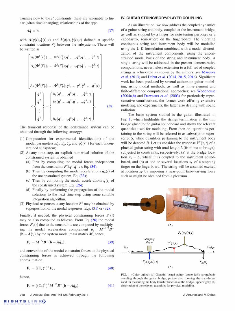
The basic system studied is the guitar illustrated in

Fig. 1, which highlights the strings termination at the thin

bridge glued to the guitar soundboard and shows the relevant

quantities used for modeling. From then on, quantities per-

taining to the string will be referred to as subscript or super-

script S, while quantities pertaining to the instrument body

will be denoted B. Let us consider the response YSðx; tÞ of a

plucked guitar string with total length L (from nut to bridge),

subjected to constraints, respectively: (a) at the bridge loca-

tion xB ¼ L, where it is coupled to the instrument sound-

board, and (b) at one or several locations xF of a stopping

finger on the fingerboard. The string will be assumed excited

at location xE by imposing a near-point time-varying force

such as might be obtained from a plectrum.

FIG. 1. (Color online) (a) Giannini tested guitar (upper left); string/body

coupling through the guitar bridge, picture also showing the transducers

used for measuring the body transfer function at the bridge (upper right); (b)

description of the relevant quantities for physical modeling.

768 J. Acoust. Soc. Am. 141 (2), February 2017 J. Antunes and V. Debut

A. String/body coupling at the bridge

The bridge is comparatively hard and massive, as com-

pared to the flexibility of both the string and soundboard,

and will therefore be treated here as a rigid transmission

interface. For small vibration amplitudes, the string and

body geometric and material nonlinearities may well be

assumed negligible, therefore, the basic unconstrained modal

Eq. (36) reads

€qSu

€qBu

( )¼ ðMSÞ�1

0

0 ðMBÞ�1

" #

� � CS 0

0 CB

" #_qS

_qB

( )

� KS 0

0 KB

" #qS

qB

( )þ FS

exc

0

( )!; (42)

where the external modal forces FSexcðtÞ stem from the string

playing, at location(s) xEðtÞ, where the excitation force

FEðxEðtÞ; tÞ is applied. No external body forces FBexcðtÞ are

considered, as the string/body coupling is formulated in

terms of a constraint equation: The bridge location xB ¼ L,

the string motion YSðxB; tÞ must be the same as the instru-

ment body motion at the string location YBð~r S; tÞ. Then, two

different cases will be studied in the following:

(a1) The body is rigid and motionless (as in a monochord):

YSðxB; tÞ ¼ 0) ðUSBÞ

TqSðtÞ ¼ 0: (43)

(a2) The body is flexible and defined in terms of its modal

basis

YSðxB; tÞ � YBð~r S; tÞ ¼ 0

) ðUSBÞ

TqSðtÞ � ðUBS Þ

TqBðtÞ ¼ 0: (44)

Obviously, in constraints (43) and (44) the modeshape vector

is taken at the relevant locations USB � USðxBÞ and

UBS � UBð~r SÞ. The modal excitation vector in Eq. (42) is

obtained by modal projection of FEðxEðtÞ; tÞ on the string

modes, as per Eqs. (29) and (30). For generality, we assume

that the excitation location(s) xEðtÞ may change in time, fol-

lowing a musician’s playing.

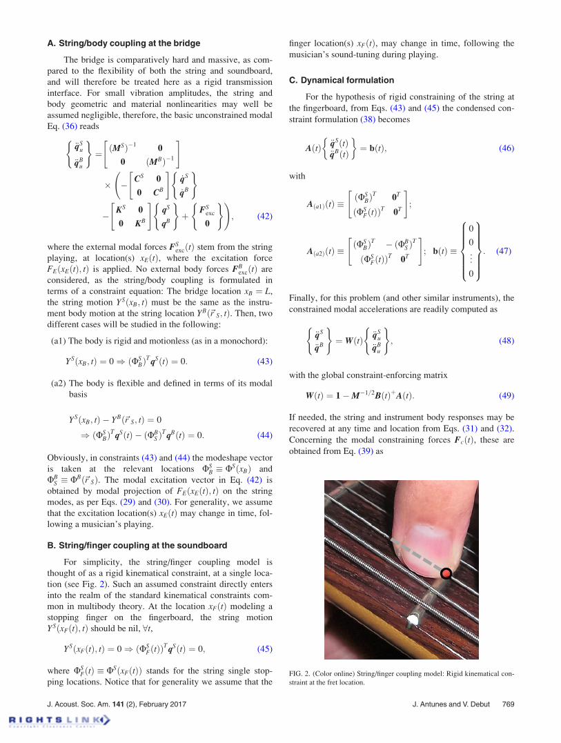
B. String/finger coupling at the soundboard

For simplicity, the string/finger coupling model is

thought of as a rigid kinematical constraint, at a single loca-

tion (see Fig. 2). Such an assumed constraint directly enters

into the realm of the standard kinematical constraints com-

mon in multibody theory. At the location xFðtÞ modeling a

stopping finger on the fingerboard, the string motion

YSðxFðtÞ; tÞ should be nil, 8t,

YSðxFðtÞ; tÞ ¼ 0) ðUSFðtÞÞ

TqSðtÞ ¼ 0; (45)

where USFðtÞ � USðxFðtÞÞ stands for the string single stop-

ping locations. Notice that for generality we assume that the

finger location(s) xFðtÞ, may change in time, following the

musician’s sound-tuning during playing.

C. Dynamical formulation

For the hypothesis of rigid constraining of the string at

the fingerboard, from Eqs. (43) and (45) the condensed con-

straint formulation (38) becomes

AðtÞ €qSðtÞ€qBðtÞ

� �¼ bðtÞ; (46)

with

Aða1ÞðtÞ �ðUS

BÞT

0T

ðUSFðtÞÞ

T0T

" #;

Aða2ÞðtÞ �ðUS

BÞT � ðUB

S ÞT

ðUSFðtÞÞ

T0T

" #; bðtÞ �

0

0

..

.

0

8>>>>><>>>>>:

9>>>>>=>>>>>;: (47)

Finally, for this problem (and other similar instruments), the

constrained modal accelerations are readily computed as

€qS

€qB

( )¼ WðtÞ €qS

u

€qBu

( ); (48)

with the global constraint-enforcing matrix

WðtÞ ¼ 1�M�1=2BðtÞþAðtÞ: (49)

If needed, the string and instrument body responses may be

recovered at any time and location from Eqs. (31) and (32).

Concerning the modal constraining forces FcðtÞ, these are

obtained from Eq. (39) as

FIG. 2. (Color online) String/finger coupling model: Rigid kinematical con-

straint at the fret location.

J. Acoust. Soc. Am. 141 (2), February 2017 J. Antunes and V. Debut 769

FSc

FBc

( )¼ ZðtÞ €qS

u

€qBu

( ); (50)

with

ZðtÞ ¼ �M1=2BðtÞþAðtÞ; (51)

and, from Eq. (50), the physical constraining forces FcðtÞ are

obtained through Eq. (40).

Notice that, if the matrix of modal constraints A is time-

independent (e.g., the stopping finger does not move), then

matrices W and Z are also constant and may be computed

once and for all, so that the constraint-enforcing equation

(48) is numerically quite efficient. Even if several different

notes are played in succession, the limited number of matri-

ces Wnote can be pre-computed prior to the time-loop, so that

obtaining the dynamical responses remains quite efficient.

Nevertheless, care should be taken when implementing

sequences of notes, in order not to enforce rigid constraints

to the string at the successive finger positions without insur-

ing a smooth transition of the string dynamics at each new

note. Such issue will be addressed elsewhere.

Obviously, any number of strings may be easily coupled

to the body by extending the relevant dynamical and con-

straint operators as appropriate, thus, modeling a complete

instrument. Then, to compute the time-domain responses,

many adequate ODE solvers may be used. Here, a simple

explicit velocity-Verlet algorithm was implemented; see, for

instance, Press et al. (2007), and details of the implementa-

tion are given in the Appendix.

V. ILLUSTRATIVE COMPUTATIONS

A. System parameters

The illustrative computations presented in the following

are based on guitar body modes experimentally identified

from a transfer function we measured at the instrument

bridge; see Fig. 1. The computed string (A2) is tuned to a

fundamental of f1 ¼ 110 Hz, with length (from nut to bridge)

L ¼ 0:65 m, axial tensioning force T ¼ 73:9 N, mass per unit

length ql ¼ 3:61� 10�3 kg=m, transverse wave propagation

velocity ct ¼ffiffiffiffiffiffiffiffiffiffiT=ql

p¼ 143 m=s, and inharmonicity parame-

ter (bending stiffness of a non-ideal string) B ¼ EI ¼ 4

�10�5 Nm2. These parameters have been taken from the

experimental work by Woodhouse (2004b). Then, for the

unconstrained string used in our dynamical computations

(pinned at the nut and “free” at the bridge), the inharmonic

modal frequencies are computed as

f Sn ¼

ct

2ppn 1þ B

2Tp2

n

� �with pn ¼

2n� 1ð Þp2L

(52)

with modeshapes:

/Sn xð Þ ¼ sin

2n� 1ð Þpx

2L

� �; (53)

and modal masses

mSn ¼ ql

ðL

0

/Sn xð Þ

h i2

dx ¼ qlL

2; 8n: (54)

Concerning the string modal damping, complex dissipative

phenomena must be accounted for, as thoroughly discussed

by Woodhouse (2004a,b), who proposed the following prag-

matic formulation for modal damping based on three loss

parameters:

fSn ¼

1

2

T gF þgA

2pf Sn

� �þ gBBp2

n

T þ Bp2n

; (55)

where the loss coefficients, somewhat loosely described as

“internal friction,” “air viscous damping,” and “bending

damping,” fitted from experimental data, are for this string

gF ¼ 7� 10�5, gA ¼ 0:9, and gB ¼ 2:5� 10�2.

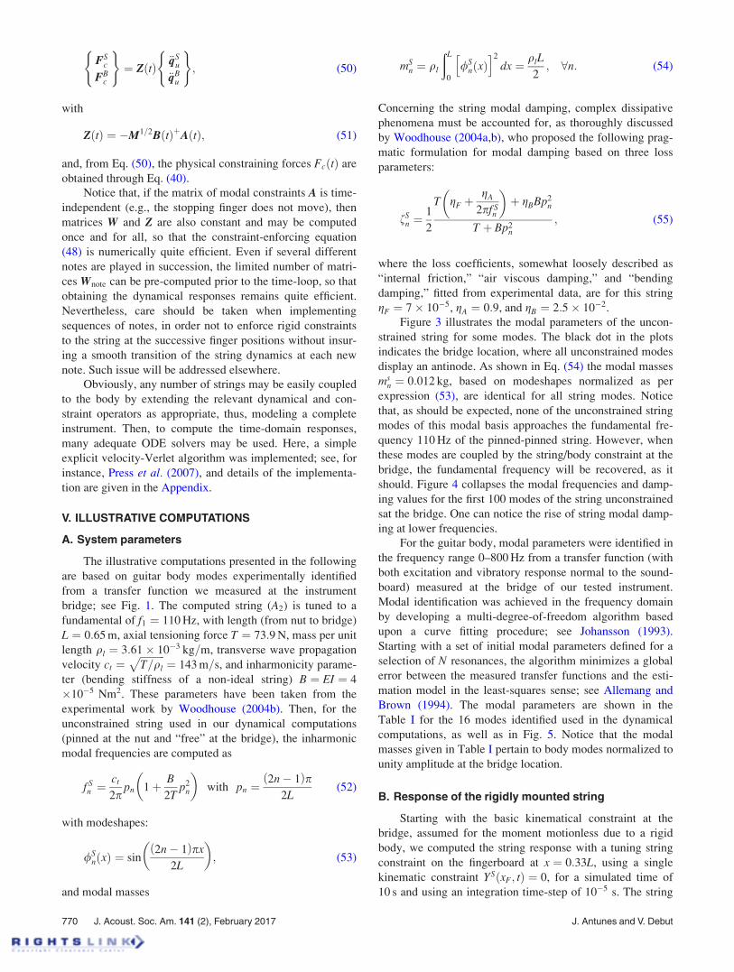
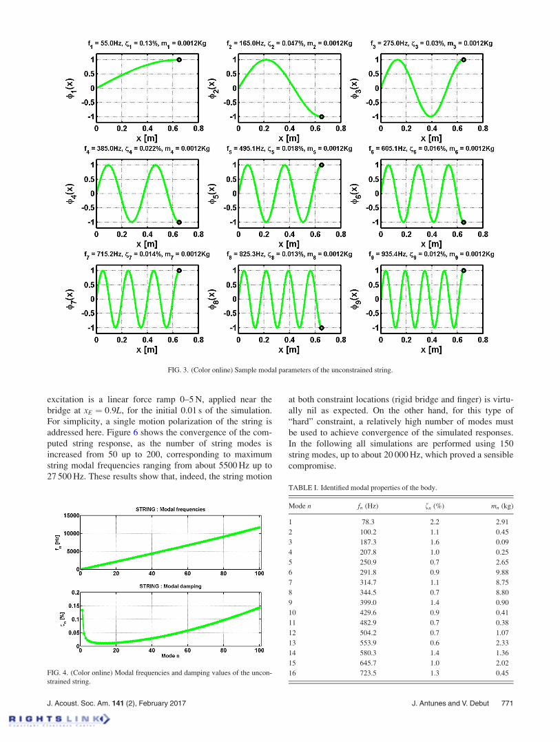
Figure 3 illustrates the modal parameters of the uncon-

strained string for some modes. The black dot in the plots

indicates the bridge location, where all unconstrained modes

display an antinode. As shown in Eq. (54) the modal masses

msn ¼ 0:012 kg, based on modeshapes normalized as per

expression (53), are identical for all string modes. Notice

that, as should be expected, none of the unconstrained string

modes of this modal basis approaches the fundamental fre-

quency 110 Hz of the pinned-pinned string. However, when

these modes are coupled by the string/body constraint at the

bridge, the fundamental frequency will be recovered, as it

should. Figure 4 collapses the modal frequencies and damp-

ing values for the first 100 modes of the string unconstrained

sat the bridge. One can notice the rise of string modal damp-

ing at lower frequencies.

For the guitar body, modal parameters were identified in

the frequency range 0–800 Hz from a transfer function (with

both excitation and vibratory response normal to the sound-

board) measured at the bridge of our tested instrument.

Modal identification was achieved in the frequency domain

by developing a multi-degree-of-freedom algorithm based

upon a curve fitting procedure; see Johansson (1993).

Starting with a set of initial modal parameters defined for a

selection of N resonances, the algorithm minimizes a global

error between the measured transfer functions and the esti-

mation model in the least-squares sense; see Allemang and

Brown (1994). The modal parameters are shown in the

Table I for the 16 modes identified used in the dynamical

computations, as well as in Fig. 5. Notice that the modal

masses given in Table I pertain to body modes normalized to

unity amplitude at the bridge location.

B. Response of the rigidly mounted string

Starting with the basic kinematical constraint at the

bridge, assumed for the moment motionless due to a rigid

body, we computed the string response with a tuning string

constraint on the fingerboard at x ¼ 0:33L, using a single

kinematic constraint YSðxF; tÞ ¼ 0, for a simulated time of

10 s and using an integration time-step of 10�5 s. The string

770 J. Acoust. Soc. Am. 141 (2), February 2017 J. Antunes and V. Debut

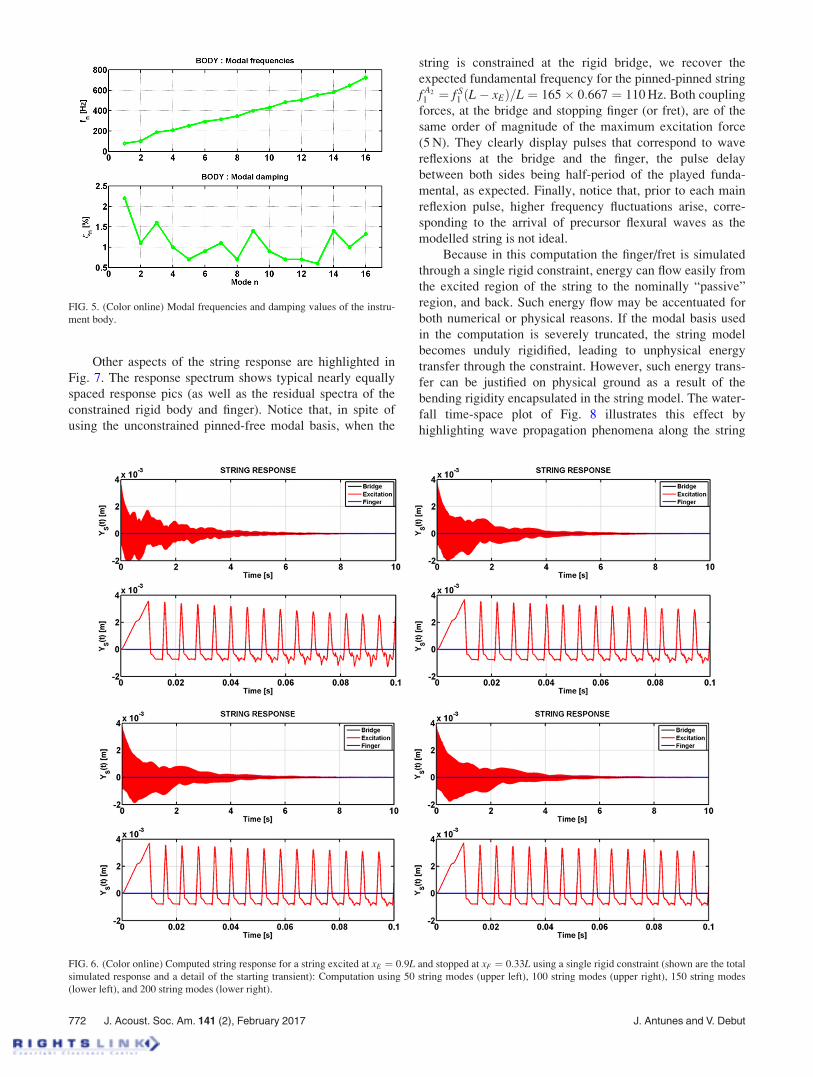
excitation is a linear force ramp 0–5 N, applied near the

bridge at xE ¼ 0:9L, for the initial 0.01 s of the simulation.

For simplicity, a single motion polarization of the string is

addressed here. Figure 6 shows the convergence of the com-

puted string response, as the number of string modes is

increased from 50 up to 200, corresponding to maximum

string modal frequencies ranging from about 5500 Hz up to

27 500 Hz. These results show that, indeed, the string motion

at both constraint locations (rigid bridge and finger) is virtu-

ally nil as expected. On the other hand, for this type of

“hard” constraint, a relatively high number of modes must

be used to achieve convergence of the simulated responses.

In the following all simulations are performed using 150

string modes, up to about 20 000 Hz, which proved a sensible

compromise.

FIG. 4. (Color online) Modal frequencies and damping values of the uncon-

strained string.

TABLE I. Identified modal properties of the body.

Mode n fn (Hz) fn (%) mn (kg)

1 78.3 2.2 2.91

2 100.2 1.1 0.45

3 187.3 1.6 0.09

4 207.8 1.0 0.25

5 250.9 0.7 2.65

6 291.8 0.9 9.88

7 314.7 1.1 8.75

8 344.5 0.7 8.80

9 399.0 1.4 0.90

10 429.6 0.9 0.41

11 482.9 0.7 0.38

12 504.2 0.7 1.07

13 553.9 0.6 2.33

14 580.3 1.4 1.36

15 645.7 1.0 2.02

16 723.5 1.3 0.45

FIG. 3. (Color online) Sample modal parameters of the unconstrained string.

J. Acoust. Soc. Am. 141 (2), February 2017 J. Antunes and V. Debut 771

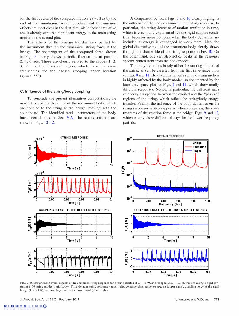
Other aspects of the string response are highlighted in

Fig. 7. The response spectrum shows typical nearly equally

spaced response pics (as well as the residual spectra of the

constrained rigid body and finger). Notice that, in spite of

using the unconstrained pinned-free modal basis, when the

string is constrained at the rigid bridge, we recover the

expected fundamental frequency for the pinned-pinned string

f A2

1 ¼ f S1 ðL� xEÞ=L ¼ 165� 0:667 ¼ 110 Hz. Both coupling

forces, at the bridge and stopping finger (or fret), are of the

same order of magnitude of the maximum excitation force

(5 N). They clearly display pulses that correspond to wave

reflexions at the bridge and the finger, the pulse delay

between both sides being half-period of the played funda-

mental, as expected. Finally, notice that, prior to each main

reflexion pulse, higher frequency fluctuations arise, corre-

sponding to the arrival of precursor flexural waves as the

modelled string is not ideal.

Because in this computation the finger/fret is simulated

through a single rigid constraint, energy can flow easily from

the excited region of the string to the nominally “passive”

region, and back. Such energy flow may be accentuated for

both numerical or physical reasons. If the modal basis used

in the computation is severely truncated, the string model

becomes unduly rigidified, leading to unphysical energy

transfer through the constraint. However, such energy trans-

fer can be justified on physical ground as a result of the

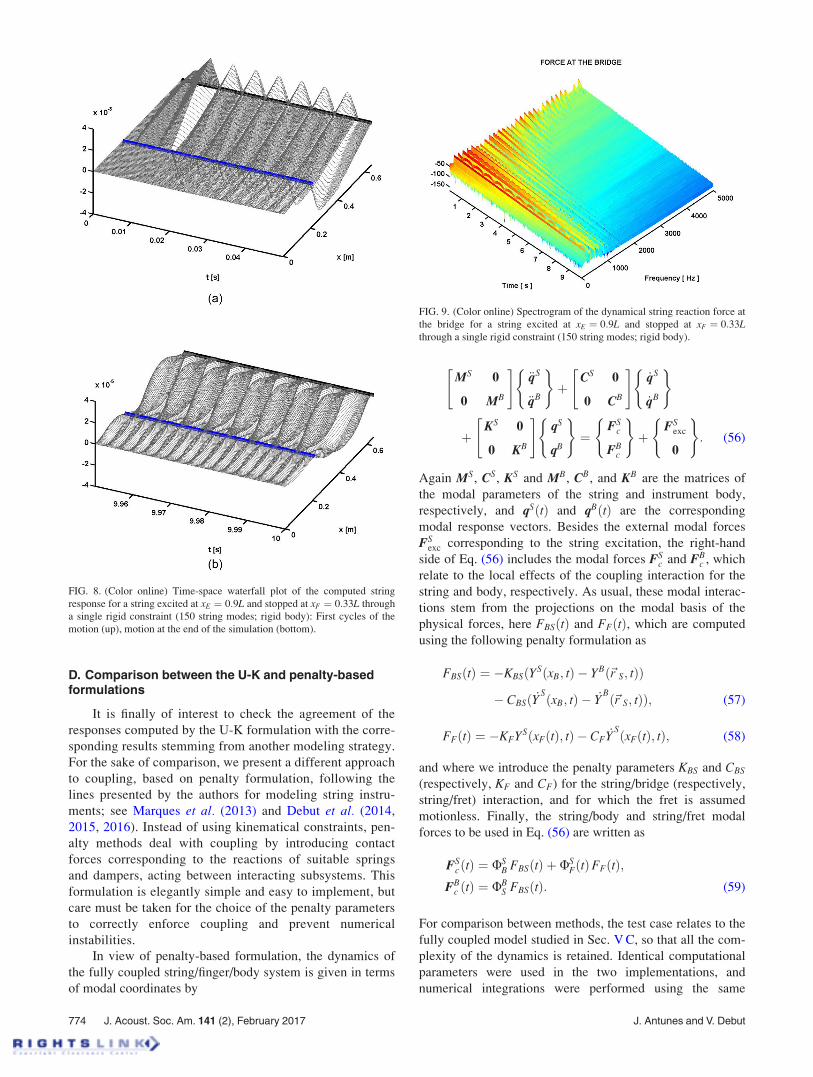
bending rigidity encapsulated in the string model. The water-

fall time-space plot of Fig. 8 illustrates this effect by

highlighting wave propagation phenomena along the string

FIG. 6. (Color online) Computed string response for a string excited at xE ¼ 0:9L and stopped at xF ¼ 0:33L using a single rigid constraint (shown are the total

simulated response and a detail of the starting transient): Computation using 50 string modes (upper left), 100 string modes (upper right), 150 string modes

(lower left), and 200 string modes (lower right).

FIG. 5. (Color online) Modal frequencies and damping values of the instru-

ment body.

772 J. Acoust. Soc. Am. 141 (2), February 2017 J. Antunes and V. Debut

for the first cycles of the computed motion, as well as by the

end of the simulation. Wave reflection and transmission

effects are most clear in the first plot, while their cumulative

result already captured significant energy to the main string

motion in the second plot.

The effects of this energy transfer may be felt by

the instrument through the dynamical string force at the

bridge. The spectrogram of the computed force shown

in Fig. 9 clearly shows periodic fluctuations at partials

2, 4, 6, etc. These are clearly related to the modes 1, 2,

3, etc. of the “passive” region, which have the same

frequencies for the chosen stopping finger location

(xF ¼ 0:33L).

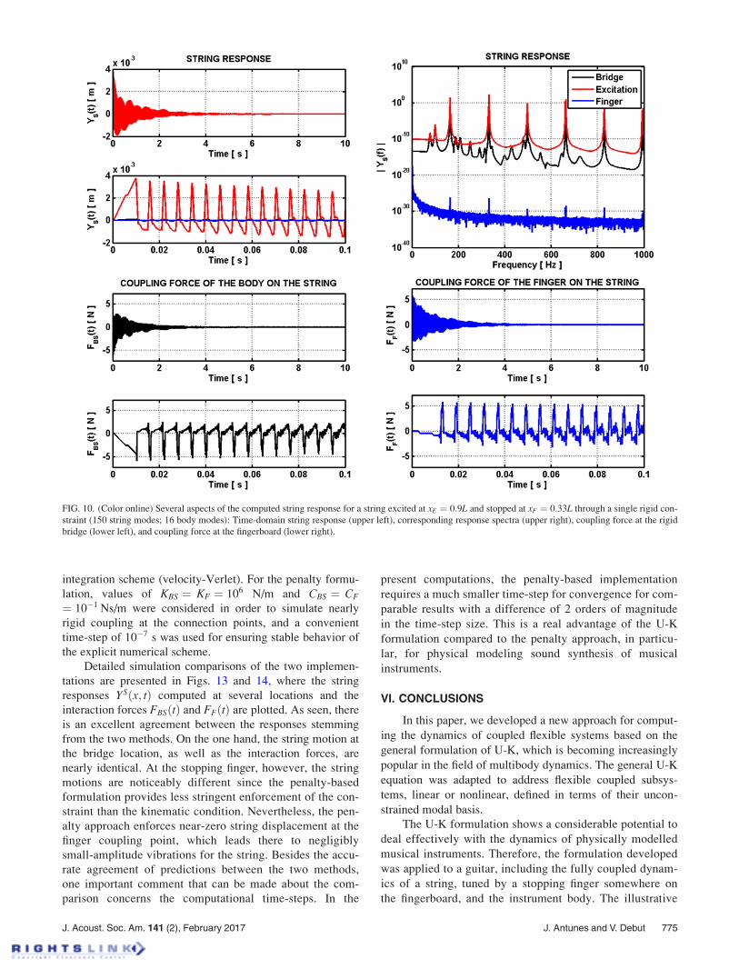
C. Influence of the string/body coupling

To conclude the present illustrative computations, we

now introduce the dynamics of the instrument body, which

are coupled to the string at the bridge, moving with the

soundboard. The identified modal parameters of the body

have been detailed in Sec. V A. The results obtained are

shown in Figs. 10–12.

A comparison between Figs. 7 and 10 clearly highlights

the influence of the body dynamics on the string response. In

particular, the string decrease of motion amplitude in time,

which is essentially exponential for the rigid support condi-

tion, becomes more complex when the body dynamics are

included as energy is exchanged between them. Also, the

global dissipative role of the instrument body clearly shows

through the shorter life of the string response in Fig. 10. On

the other hand, one can also notice peaks in the response

spectra, which stem from the body modes.

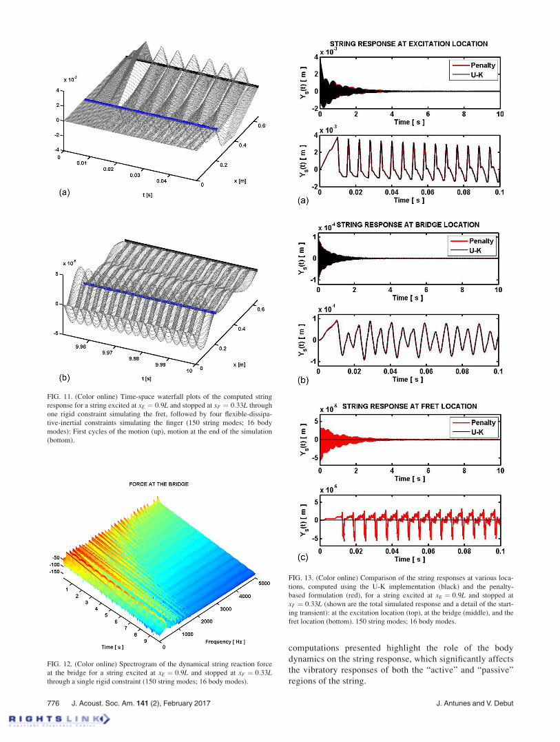
The body dynamics barely affect the starting motion of

the string, as can be asserted from the first time-space plots

of Figs. 8 and 11. However, in the long run, the string motion

is highly affected by the body modes, as documented by the

later time-space plots of Figs. 8 and 11, which show totally

different responses. Notice, in particular, the different rates

of energy dissipation between the excited and the “passive”

regions of the string, which reflect the string/body energy

transfer. Finally, the influence of the body dynamics on the

string responses is also supported when comparing the spec-

trograms of the reaction force at the bridge, Figs. 9 and 12,

which clearly show different decays for the lower frequency

partials.

FIG. 7. (Color online) Several aspects of the computed string response for a string excited at xE ¼ 0:9L and stopped at xF ¼ 0:33L through a single rigid con-

straint (150 string modes; rigid body): Time-domain string response (upper left), corresponding response spectra (upper right), coupling force at the rigid

bridge (lower left), and coupling force at the fingerboard (lower right).

J. Acoust. Soc. Am. 141 (2), February 2017 J. Antunes and V. Debut 773

D. Comparison between the U-K and penalty-basedformulations

It is finally of interest to check the agreement of the

responses computed by the U-K formulation with the corre-

sponding results stemming from another modeling strategy.

For the sake of comparison, we present a different approach

to coupling, based on penalty formulation, following the

lines presented by the authors for modeling string instru-

ments; see Marques et al. (2013) and Debut et al. (2014,

2015, 2016). Instead of using kinematical constraints, pen-

alty methods deal with coupling by introducing contact

forces corresponding to the reactions of suitable springs

and dampers, acting between interacting subsystems. This

formulation is elegantly simple and easy to implement, but

care must be taken for the choice of the penalty parameters

to correctly enforce coupling and prevent numerical

instabilities.

In view of penalty-based formulation, the dynamics of

the fully coupled string/finger/body system is given in terms

of modal coordinates by

MS 0

0 MB

" #€qS

€qB

( )þ

CS 0

0 CB

" #_qS

_qB

( )

þKS 0

0 KB

" #qS

qB

( )¼

FSc

FBc

( )þ

FSexc

0

( ): (56)

Again MS, CS, KS and MB, CB, and KB are the matrices of

the modal parameters of the string and instrument body,

respectively, and qSðtÞ and qBðtÞ are the corresponding

modal response vectors. Besides the external modal forces

FSexc corresponding to the string excitation, the right-hand

side of Eq. (56) includes the modal forces FSc and FB

c , which

relate to the local effects of the coupling interaction for the

string and body, respectively. As usual, these modal interac-

tions stem from the projections on the modal basis of the

physical forces, here FBSðtÞ and FFðtÞ, which are computed

using the following penalty formulation as

FBSðtÞ ¼ �KBSðYSðxB; tÞ � YBð~r S; tÞÞ

� CBSð _YSðxB; tÞ � _Y

Bð~r S; tÞÞ; (57)

FFðtÞ ¼ �KFYSðxFðtÞ; tÞ � CF_Y

SðxFðtÞ; tÞ; (58)

and where we introduce the penalty parameters KBS and CBS

(respectively, KF and CF) for the string/bridge (respectively,

string/fret) interaction, and for which the fret is assumed

motionless. Finally, the string/body and string/fret modal

forces to be used in Eq. (56) are written as

FScðtÞ ¼ US

B FBSðtÞ þ USFðtÞFFðtÞ;

FBc ðtÞ ¼ UB

S FBSðtÞ: (59)

For comparison between methods, the test case relates to the

fully coupled model studied in Sec. V C, so that all the com-

plexity of the dynamics is retained. Identical computational

parameters were used in the two implementations, and

numerical integrations were performed using the same

FIG. 9. (Color online) Spectrogram of the dynamical string reaction force at

the bridge for a string excited at xE ¼ 0:9L and stopped at xF ¼ 0:33Lthrough a single rigid constraint (150 string modes; rigid body).

FIG. 8. (Color online) Time-space waterfall plot of the computed string

response for a string excited at xE ¼ 0:9L and stopped at xF ¼ 0:33L through

a single rigid constraint (150 string modes; rigid body): First cycles of the

motion (up), motion at the end of the simulation (bottom).

774 J. Acoust. Soc. Am. 141 (2), February 2017 J. Antunes and V. Debut

integration scheme (velocity-Verlet). For the penalty formu-

lation, values of KBS ¼ KF ¼ 106 N/m and CBS ¼ CF

¼ 10�1 Ns/m were considered in order to simulate nearly

rigid coupling at the connection points, and a convenient

time-step of 10�7 s was used for ensuring stable behavior of

the explicit numerical scheme.

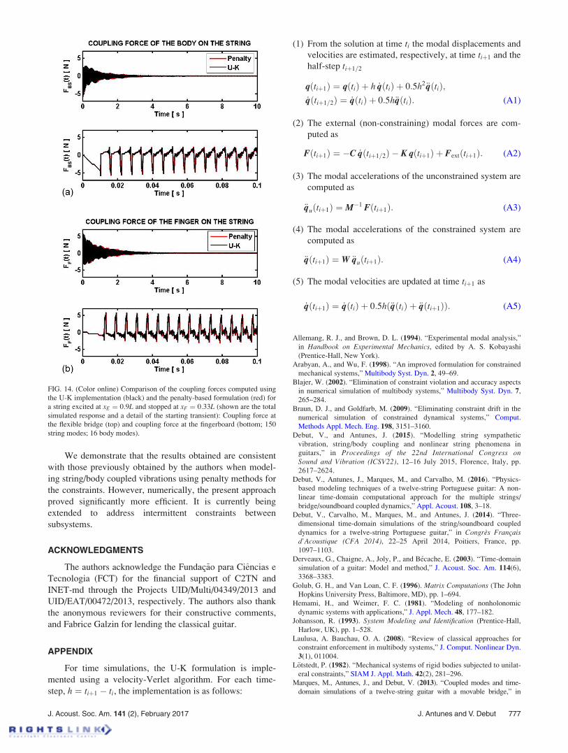
Detailed simulation comparisons of the two implemen-

tations are presented in Figs. 13 and 14, where the string

responses YSðx; tÞ computed at several locations and the

interaction forces FBSðtÞ and FFðtÞ are plotted. As seen, there

is an excellent agreement between the responses stemming

from the two methods. On the one hand, the string motion at

the bridge location, as well as the interaction forces, are

nearly identical. At the stopping finger, however, the string

motions are noticeably different since the penalty-based

formulation provides less stringent enforcement of the con-

straint than the kinematic condition. Nevertheless, the pen-

alty approach enforces near-zero string displacement at the

finger coupling point, which leads there to negligibly

small-amplitude vibrations for the string. Besides the accu-

rate agreement of predictions between the two methods,

one important comment that can be made about the com-

parison concerns the computational time-steps. In the

present computations, the penalty-based implementation

requires a much smaller time-step for convergence for com-

parable results with a difference of 2 orders of magnitude

in the time-step size. This is a real advantage of the U-K

formulation compared to the penalty approach, in particu-

lar, for physical modeling sound synthesis of musical

instruments.

VI. CONCLUSIONS

In this paper, we developed a new approach for comput-

ing the dynamics of coupled flexible systems based on the

general formulation of U-K, which is becoming increasingly

popular in the field of multibody dynamics. The general U-K

equation was adapted to address flexible coupled subsys-

tems, linear or nonlinear, defined in terms of their uncon-

strained modal basis.

The U-K formulation shows a considerable potential to

deal effectively with the dynamics of physically modelled

musical instruments. Therefore, the formulation developed

was applied to a guitar, including the fully coupled dynam-

ics of a string, tuned by a stopping finger somewhere on

the fingerboard, and the instrument body. The illustrative

FIG. 10. (Color online) Several aspects of the computed string response for a string excited at xE ¼ 0:9L and stopped at xF ¼ 0:33L through a single rigid con-

straint (150 string modes; 16 body modes): Time-domain string response (upper left), corresponding response spectra (upper right), coupling force at the rigid

bridge (lower left), and coupling force at the fingerboard (lower right).

J. Acoust. Soc. Am. 141 (2), February 2017 J. Antunes and V. Debut 775

computations presented highlight the role of the body

dynamics on the string response, which significantly affects

the vibratory responses of both the “active” and “passive”

regions of the string.

FIG. 11. (Color online) Time-space waterfall plots of the computed string

response for a string excited at xE ¼ 0:9L and stopped at xF ¼ 0:33L through

one rigid constraint simulating the fret, followed by four flexible-dissipa-

tive-inertial constraints simulating the finger (150 string modes; 16 body

modes): First cycles of the motion (up), motion at the end of the simulation

(bottom).

FIG. 12. (Color online) Spectrogram of the dynamical string reaction force

at the bridge for a string excited at xE ¼ 0:9L and stopped at xF ¼ 0:33Lthrough a single rigid constraint (150 string modes; 16 body modes).

FIG. 13. (Color online) Comparison of the string responses at various loca-

tions, computed using the U-K implementation (black) and the penalty-

based formulation (red), for a string excited at xE ¼ 0:9L and stopped at

xF ¼ 0:33L (shown are the total simulated response and a detail of the start-

ing transient): at the excitation location (top), at the bridge (middle), and the

fret location (bottom). 150 string modes; 16 body modes.

776 J. Acoust. Soc. Am. 141 (2), February 2017 J. Antunes and V. Debut

We demonstrate that the results obtained are consistent

with those previously obtained by the authors when model-

ing string/body coupled vibrations using penalty methods for

the constraints. However, numerically, the present approach

proved significantly more efficient. It is currently being

extended to address intermittent constraints between

subsystems.

ACKNOWLEDGMENTS

The authors acknowledge the Fundac~ao para Ciencias e

Tecnologia (FCT) for the financial support of C2TN and

INET-md through the Projects UID/Multi/04349/2013 and

UID/EAT/00472/2013, respectively. The authors also thank

the anonymous reviewers for their constructive comments,

and Fabrice Galzin for lending the classical guitar.

APPENDIX

For time simulations, the U-K formulation is imple-

mented using a velocity-Verlet algorithm. For each time-

step, h ¼ tiþ1 � ti, the implementation is as follows:

(1) From the solution at time ti the modal displacements and

velocities are estimated, respectively, at time tiþ1 and the

half-step tiþ1=2

qðtiþ1Þ ¼ qðtiÞ þ h _qðtiÞ þ 0:5h2€qðtiÞ;_qðtiþ1=2Þ ¼ _qðtiÞ þ 0:5h€qðtiÞ: (A1)

(2) The external (non-constraining) modal forces are com-

puted as

Fðtiþ1Þ ¼ �C _qðtiþ1=2Þ � K qðtiþ1Þ þ Fextðtiþ1Þ: (A2)

(3) The modal accelerations of the unconstrained system are

computed as

€quðtiþ1Þ ¼ M�1 Fðtiþ1Þ: (A3)

(4) The modal accelerations of the constrained system are

computed as

€qðtiþ1Þ ¼ W €quðtiþ1Þ: (A4)

(5) The modal velocities are updated at time tiþ1 as

_qðtiþ1Þ ¼ _qðtiÞ þ 0:5hð€qðtiÞ þ €qðtiþ1ÞÞ: (A5)

Allemang, R. J., and Brown, D. L. (1994). “Experimental modal analysis,”

in Handbook on Experimental Mechanics, edited by A. S. Kobayashi

(Prentice-Hall, New York).

Arabyan, A., and Wu, F. (1998). “An improved formulation for constrained

mechanical systems,” Multibody Syst. Dyn. 2, 49–69.

Blajer, W. (2002). “Elimination of constraint violation and accuracy aspects

in numerical simulation of multibody systems,” Multibody Syst. Dyn. 7,

265–284.

Braun, D. J., and Goldfarb, M. (2009). “Eliminating constraint drift in the

numerical simulation of constrained dynamical systems,” Comput.

Methods Appl. Mech. Eng. 198, 3151–3160.

Debut, V., and Antunes, J. (2015). “Modelling string sympathetic

vibration, string/body coupling and nonlinear string phenomena in

guitars,” in Proceedings of the 22nd International Congress onSound and Vibration (ICSV22), 12–16 July 2015, Florence, Italy, pp.

2617–2624.

Debut, V., Antunes, J., Marques, M., and Carvalho, M. (2016). “Physics-

based modeling techniques of a twelve-string Portuguese guitar: A non-

linear time-domain computational approach for the multiple strings/

bridge/soundboard coupled dynamics,” Appl. Acoust. 108, 3–18.

Debut, V., Carvalho, M., Marques, M., and Antunes, J. (2014). “Three-

dimensional time-domain simulations of the string/soundboard coupled

dynamics for a twelve-string Portuguese guitar,” in Congres Francaisd’Acoustique (CFA 2014), 22–25 April 2014, Poitiers, France, pp.

1097–1103.

Derveaux, G., Chaigne, A., Joly, P., and B�ecache, E. (2003). “Time-domain

simulation of a guitar: Model and method,” J. Acoust. Soc. Am. 114(6),

3368–3383.

Golub, G. H., and Van Loan, C. F. (1996). Matrix Computations (The John

Hopkins University Press, Baltimore, MD), pp. 1–694.

Hemami, H., and Weimer, F. C. (1981). “Modeling of nonholonomic

dynamic systems with applications,” J. Appl. Mech. 48, 177–182.

Johansson, R. (1993). System Modeling and Identification (Prentice-Hall,

Harlow, UK), pp. 1–528.

Laulusa, A. Bauchau, O. A. (2008). “Review of classical approaches for

constraint enforcement in multibody systems,” J. Comput. Nonlinear Dyn.

3(1), 011004.

L€otstedt, P. (1982). “Mechanical systems of rigid bodies subjected to unilat-

eral constraints,” SIAM J. Appl. Math. 42(2), 281–296.

Marques, M., Antunes, J., and Debut, V. (2013). “Coupled modes and time-

domain simulations of a twelve-string guitar with a movable bridge,” in

FIG. 14. (Color online) Comparison of the coupling forces computed using

the U-K implementation (black) and the penalty-based formulation (red) for

a string excited at xE ¼ 0:9L and stopped at xF ¼ 0:33L (shown are the total

simulated response and a detail of the starting transient): Coupling force at

the flexible bridge (top) and coupling force at the fingerboard (bottom; 150

string modes; 16 body modes).

J. Acoust. Soc. Am. 141 (2), February 2017 J. Antunes and V. Debut 777

Stockholm Music Acoustics Conference (SMAC 2013), edited by R. Bresin

and A. Askenfeldt, 30 July–3 August 2013, Stockholm, Sweden, pp.

633–640.

Pennestri, E., Valentini, P. P., and de Falco, D. (2010). “An application of

the Udwadia-Kalaba dynamic formulation to flexible multibody systems,”

J. Franklin Inst. 347, 173–194.

Press, W. H., Teukolsky, S. A., Vetterling, W. T., and Flannery, B. P.

(2007). Numerical Recipes: The Art of Scientific Computing (Cambridge

University Press, New York), pp. 1–1256.

Shabana, A. A. (2010). Computational Dynamics (Wiley, Chichester, UK),

pp. 1–542.

Udwadia, F. E. (1996). “Equations of motion for mechanical systems: A uni-

fied approach,” Int. J. Nonlinear Mech. 31(6), 951–958.

Udwadia, F. E., and Kalaba, R. E. (1992). “A new perspective on constrained

motion,” Proc. R. Soc. London A 439, 407–410.

Udwadia, F. E., and Kalaba, R. E. (1996). Analytical Dynamics—A NewApproach (Cambridge University Press, New York), pp. 1–276.

Udwadia, F. E., and Kalaba, R. E. (2000). “Nonideal constraints and

Lagrangian dynamics,” J. Aerospace Eng. 13, 17–22.

Udwadia, F. E., and Phohomsiri, P. (2006). “Explicit equations of motion

for constrained mechanical systems with singular mass matrices and appli-

cations to multi-body dynamics,” Proc. R. Soc. London A 462,

2097–2117.

Woodhouse, J. (2004a). “On the synthesis of guitar plucks,” Acta Acust.

associated Ac. 90, 928–944.

Woodhouse, J. (2004b). “Plucked guitar transients: Comparison of measure-

ments and synthesis,” Acta Acust. associated Ac. 90, 945–965.

Yoon, S., Howe, R. M., and Greenwood, D. T. (1994). “Geometric elimina-

tion of constraint violations in numerical simulation of Lagrangian equa-

tions,” J. Mech. Design 116, 1058–1064.

778 J. Acoust. Soc. Am. 141 (2), February 2017 J. Antunes and V. Debut