Embed Size (px)
Citation preview
University of UdineDepartment of Mathematics and Computer Science
University Joseph Fourier - Grenoble IMSTII Doctoral School
Reachability Computation and Parameter
Synthesis for Polynomial Dynamical
Systems
Tommaso Dreossi
Jury
Carla Piazza President, directorThao Dang Examiner, directorSebastiano Battiato ExaminerSabina Rossi ExaminerSriram Sankaranarayanan ReviewerRadu Grosu Reviewer

ii

Acknowledgements
I would like to acknowledge some people who contributed to the development of thiswork.
First, I would like to thank my advisors. I thank Carla Piazza for introducing me tothe research world and advising me. Thanks to her teachings and approach to science,I learned how to explore topics more deeply and to be more precise in what I do. Herguidance and fruitful suggestions helped me a lot, especially with the development ofthis work. I am grateful to Thao Dang; I thank her for conveying to me the passion forresearch and investigation. Her endless positivity and optimism have given me a sereneapproach to research. Thanks to her, I learned to enjoy every aspect of this work andunderstood how lucky I am to be a researcher. I really thank both of you for beingconstant, present, and patient mentors who have always supported me along this path.
I am grateful to Sriram Sankaranarayanan and Radu Grosu who reviewed this workand provided me with useful comments, improvements, and ideas for future develop-ments.
During my Ph.D., I met people who influenced and inspired me. Among these peopleis Oded Maler; his creativity, passion for investigation, and irony made me understand,more deeply, the beauty of science and delights derived from it. I thank him for thestimulating discussions we had and his constant flow of reading suggestions. A greatlearning experience during my studies has been being an intern at Toyota. I want tothank Jim Kapinski, Jyo Deshmukh, and Xiaoqing Jin for giving me the opportunity ofworking with them and introducing me to real-world industrial problems.
Finally, I thank all the officemates, colleagues, and friends with whom I have sharedthis journey. And of course, I would like to thank my family, without whose supportand love none of this would have been possible.
Tommaso Dreossi

AbstractEnglish
Dynamical systems are important mathematical models used to describe the temporalevolution of systems. Often dynamical systems are equipped with parameters thatallow the models to better capture the characteristics of the abstracted phenomena. Animportant question around dynamical systems is to formally determine whether a model(biased by its parameters) behaves well.
In this thesis we deal with two main questions concerning discrete-time polynomialdynamical systems: 1) the reachability computation problem, i.e, given a set of initialconditions and a set of parameters, compute the set of states reachable by the system ina bounded time horizon; 2) the parameter synthesis problem, i.e., given a set of initialconditions, a set of parameters, and a specification, find the largest set of parameterssuch that all the behaviors of the system staring from the set of initial conditions satisfythe specification.
The reachability computation problem for nonlinear dynamical systems is well knownfor being nontrivial. Difficulties arise in handling and representing sets generated bynonlinear transformations. In this thesis we adopt a common technique that consists inover-approximating the complex reachable sets with sets that are easy to manipulate.The challenge is to determine accurate over-approximations. We propose methods tofinely over-approximate the images of sets using boxes, parallelotopes, and a new datastructure called parallelotope bundles (that are collections of parallelotopes whose in-tersections symbolically represent polytopes). These approximation techniques are thebasic steps of our reachability algorithm.
The synthesis of parameters aims at determining the values of the parameters suchthat the system behaves as expected. This feature can be used, for instance, to tune amodel so that it imitates the modeled phenomenon with a sufficient level of precision.The contributions of this thesis concerning the parameter synthesis problem are twofold.Firstly, we define a new semantics for the Signal Temporal Logic (STL) that allows oneto formalize a specification and reason on sets of parameters and flows of behaviors. Sec-ondly, we define an algorithm to compute the synthesis semantics of a formula against adiscrete-time dynamical system. The result of the algorithm constitutes a conservativesolution of the parameter synthesis problem. The developed methods for both reacha-bility computation and parameter synthesis exploit and improve Bernstein coefficientscomputation.
The techniques defined in this thesis have been implemented in a tool called Sapo.The effectiveness of our methods is validated by the application of our tool to severalpolynomial dynamical systems.

AbstractFrench
Les systemes dynamiques sont des importants modeles mathematiques utilises pourdecrire l’evolution temporelle d’un processus physique. Souvent, les systemes dynamiquessont equipes des parametres qui permettent aux modeles de mieux saisir les caracteri-stiques observees des phenomenes. Une question importante est celle de determinerformellement si un modele parametrique peut reproduire des comportement observes ousatisfait une propriete.
Dans cette these, nous traitons deux questions concernant les systemes dynamiquespolynomiaux a temps discret: 1) Calcul d’atteignabilite, i.e, etant donne un ensemblede conditions initiales et un ensemble de parametres, calculer l’ensemble d’etats at-teignables par le systeme dans un horizon de temps borne; 2) Synthese de parametres,i.e., etant donne un ensemble de conditions initiales, un ensemble de parametres, et unespecification, trouver le plus grand ensemble de parametres tel que tous les comporte-ments du systeme a partir de l’ensemble de conditions initiales satisfont la specification.
Le calcul d’atteignabilite pour les systemes dynamiques non-lineaires est bien connupour etre un probleme difficile. Des difficultes surgissent dans le traitement et la re-presentation des ensembles generes par des transformations non-lineaires. Dans cettethese, nous adoptons une technique qui consiste a approximer des ensembles d’etatsatteignables complexes par des ensembles qui sont plus faciles a manipuler. Le defiest de garantir une bonne precision d’approximation. Nous proposons des methodespour approximer les images des ensembles par des polynomiaux en utilisant des boıtes,des parallelotopes, et une nouvelle structure appelees ”parallelotope bundle” (qui sontdes collections de parallelotopes dont les intersections representent symboliquement despolytopes). Ces techniques d’approximation sont les etapes de base de notre algorithmede calcul d’atteignabilite.
La synthese de parametres vise a determiner les valeurs des parametres telles que lesysteme se comporte comme prevu. Cette fonctionnalite peut etre utilisee, par exemple,pour ajuster un modele de sorte qu’il imite le phenomene avec un degre de precisionsuffisant. Les contributions de cette these concernant le probleme de la synthese deparametres comprennent deux volets. Premierement, nous definissons une nouvellesemantique pour la logique STL ”Signal Temporal Logic” permettant de formaliser unespecification et de raisonner sur des ensembles de parametres et les flux de trajectoires.Deuxiemement, nous definissons un algorithme pour calculer la semantique de synthesed’une formule par rapport a un systeme dynamique. Le resultat de l’algorithme con-stitue une solution du probleme de la synthese de parametres. Les methodes mises aupoint pour le calcul d’atteignabilite et la synthese de parametres exploitent et ameliorentle calcul des coefficients de Bernstein des polynomiaux.
Les techniques definies dans cette these ont ete implantees dans un outil appele Sapo.L’efficacite de nos methodes est validee par l’application de notre outil a plusieurs cas.

Contents
1 Introduction 11.1 Motivations . . . . . . . . . . . . . . . . . . . . . . . . . . . . . . . . . . 1
1.1.1 Models . . . . . . . . . . . . . . . . . . . . . . . . . . . . . . . . 11.1.2 Dynamical Systems . . . . . . . . . . . . . . . . . . . . . . . . . . 21.1.3 Reachability . . . . . . . . . . . . . . . . . . . . . . . . . . . . . . 51.1.4 Parameter Synthesis . . . . . . . . . . . . . . . . . . . . . . . . . 6
1.2 Related Works . . . . . . . . . . . . . . . . . . . . . . . . . . . . . . . . 71.2.1 Reachability . . . . . . . . . . . . . . . . . . . . . . . . . . . . . . 81.2.2 Parameter Synthesis . . . . . . . . . . . . . . . . . . . . . . . . . 9
1.3 Contributions . . . . . . . . . . . . . . . . . . . . . . . . . . . . . . . . . 101.3.1 Reachability Analysis . . . . . . . . . . . . . . . . . . . . . . . . 101.3.2 Parameter Synthesis . . . . . . . . . . . . . . . . . . . . . . . . . 121.3.3 Tool Implementation . . . . . . . . . . . . . . . . . . . . . . . . . 12
1.4 Structure of the Thesis . . . . . . . . . . . . . . . . . . . . . . . . . . . . 13
2 Dynamical Systems and Parameters 152.1 Dynamical Systems . . . . . . . . . . . . . . . . . . . . . . . . . . . . . . 15
2.1.1 Parametric Continuous-Time Dynamical Systems . . . . . . . . . 162.1.2 Discrete-Time Dynamical Systems . . . . . . . . . . . . . . . . . 17
2.2 Parameter Synthesis Problem . . . . . . . . . . . . . . . . . . . . . . . . 192.2.1 The Parameter Synthesis Problem . . . . . . . . . . . . . . . . . 21
2.3 Two Important Questions . . . . . . . . . . . . . . . . . . . . . . . . . . 21
3 Parametric Reachability 233.1 Parametric Reachability Problem . . . . . . . . . . . . . . . . . . . . . . 233.2 Numerical Integration . . . . . . . . . . . . . . . . . . . . . . . . . . . . 253.3 Reachability Methods . . . . . . . . . . . . . . . . . . . . . . . . . . . . 26
3.3.1 Trajectory-Based Reachability . . . . . . . . . . . . . . . . . . . 263.3.2 Set-Based Reachability . . . . . . . . . . . . . . . . . . . . . . . . 27
3.4 (Un)Decidability . . . . . . . . . . . . . . . . . . . . . . . . . . . . . . . 28
4 Set Image Computation 314.1 Single Step Reachable Set Approximation . . . . . . . . . . . . . . . . . 31
4.1.1 Polytopes . . . . . . . . . . . . . . . . . . . . . . . . . . . . . . . 324.1.2 Polytope-Based Set Image . . . . . . . . . . . . . . . . . . . . . . 33
4.2 Bounding Polynomials . . . . . . . . . . . . . . . . . . . . . . . . . . . . 35
x Contents
4.2.1 Bernstein Basis and Coefficients . . . . . . . . . . . . . . . . . . 354.2.2 Parametric Bernstein Basis and Coefficients . . . . . . . . . . . . 394.2.3 Computation of upper bound and lower bound . . . . . . . . . . 404.2.4 Summary . . . . . . . . . . . . . . . . . . . . . . . . . . . . . . . 42
4.3 Boxes . . . . . . . . . . . . . . . . . . . . . . . . . . . . . . . . . . . . . 424.3.1 Box-Based Set Image . . . . . . . . . . . . . . . . . . . . . . . . 43
4.4 Parallelotopes . . . . . . . . . . . . . . . . . . . . . . . . . . . . . . . . . 464.4.1 Representation Conversion . . . . . . . . . . . . . . . . . . . . . 484.4.2 Parallelotope-Based Set Image . . . . . . . . . . . . . . . . . . . 49
4.5 Parallelotope Bundles . . . . . . . . . . . . . . . . . . . . . . . . . . . . 534.5.1 Bundle Data Structure . . . . . . . . . . . . . . . . . . . . . . . . 594.5.2 Bundle-Based Set Image . . . . . . . . . . . . . . . . . . . . . . . 62
4.6 Bernstein Coefficients Computation . . . . . . . . . . . . . . . . . . . . . 674.6.1 Improving Efficiency . . . . . . . . . . . . . . . . . . . . . . . . . 674.6.2 Symbolic Coefficients . . . . . . . . . . . . . . . . . . . . . . . . . 724.6.3 Improving Precision . . . . . . . . . . . . . . . . . . . . . . . . . 75
5 Parameter Synthesis 795.1 Signal Temporal Logic . . . . . . . . . . . . . . . . . . . . . . . . . . . . 795.2 STL Synthesis Semantics . . . . . . . . . . . . . . . . . . . . . . . . . . 85
5.2.1 (Un)Decidability . . . . . . . . . . . . . . . . . . . . . . . . . . . 895.3 Synthesis Algorithm . . . . . . . . . . . . . . . . . . . . . . . . . . . . . 90
5.3.1 Overall Structure . . . . . . . . . . . . . . . . . . . . . . . . . . . 915.3.2 Until Synthesis . . . . . . . . . . . . . . . . . . . . . . . . . . . . 925.3.3 Shortcuts . . . . . . . . . . . . . . . . . . . . . . . . . . . . . . . 955.3.4 Correctness and Complexity . . . . . . . . . . . . . . . . . . . . . 97
5.4 The Polynomial Case . . . . . . . . . . . . . . . . . . . . . . . . . . . . . 995.4.1 Parameter Set Representation and Manipulation . . . . . . . . . 1005.4.2 Single Step Evolution . . . . . . . . . . . . . . . . . . . . . . . . 1005.4.3 Basic Refinement . . . . . . . . . . . . . . . . . . . . . . . . . . . 101
6 Tool and Experimental Results 1096.1 Architecture . . . . . . . . . . . . . . . . . . . . . . . . . . . . . . . . . . 109
6.1.1 Sapo . . . . . . . . . . . . . . . . . . . . . . . . . . . . . . . . . . 1106.1.2 STL . . . . . . . . . . . . . . . . . . . . . . . . . . . . . . . . . . 1116.1.3 Model . . . . . . . . . . . . . . . . . . . . . . . . . . . . . . . . . 1126.1.4 Base Converter . . . . . . . . . . . . . . . . . . . . . . . . . . . . 1126.1.5 Bundle . . . . . . . . . . . . . . . . . . . . . . . . . . . . . . . . . 1126.1.6 Parallelotope . . . . . . . . . . . . . . . . . . . . . . . . . . . . . 1136.1.7 Variables Generator . . . . . . . . . . . . . . . . . . . . . . . . . 1136.1.8 Linear System Set . . . . . . . . . . . . . . . . . . . . . . . . . . 1136.1.9 Linear System . . . . . . . . . . . . . . . . . . . . . . . . . . . . 114
6.2 Case Studies . . . . . . . . . . . . . . . . . . . . . . . . . . . . . . . . . 1146.2.1 Test System . . . . . . . . . . . . . . . . . . . . . . . . . . . . . . 1146.2.2 SIR Epidemic Model . . . . . . . . . . . . . . . . . . . . . . . . . 1156.2.3 Influenza . . . . . . . . . . . . . . . . . . . . . . . . . . . . . . . 1196.2.4 Ebola . . . . . . . . . . . . . . . . . . . . . . . . . . . . . . . . . 120

Contents xi
6.2.5 Honeybees Site Choice . . . . . . . . . . . . . . . . . . . . . . . . 1236.2.6 Quadcopter . . . . . . . . . . . . . . . . . . . . . . . . . . . . . . 125
6.3 Related Tools . . . . . . . . . . . . . . . . . . . . . . . . . . . . . . . . . 128
7 Conclusion 1297.1 Thesis Overview . . . . . . . . . . . . . . . . . . . . . . . . . . . . . . . 1297.2 Further Developments . . . . . . . . . . . . . . . . . . . . . . . . . . . . 130

1Introduction
1.1 Motivations
1.1.1 Models
A model is a simplified representation of something that is real, that is not the sameas the modeled thing, but hopefully it is enough precise to be useful. A mathematicalmodel is a model described by a mathematical formalism.
Since ancient times, humans used mathematical models to represent and simplifythe real world aiming to understand the complexity of the surrounding events. Forinstance, numbers, appeared for the first time around 30.000 BC, were probably thefirst mathematical model used to abstract a quantity observable in real life. Since then,many areas benefited of mathematical abstraction and several milestones in humanknowledge were achieved with the help of models. Some examples [173] are given byEratosthenes of Cyrene (around 250 BC), who approximated the circumference of theEarth with a geometrical model, Ptolemy (around 150 AD) who used circles to predictthe movement of planets, or Giotto di Bondone and Filippo Brunelleschi (around 1300AD) who exploited geometry to abstract and picture the reality giving birth to theperspective.
Nowadays numerous domains benefit of mathematical models. Besides the classicnatural and engineering disciplines, such as physics, mechanical engineering, and biol-ogy, models find application also in relatively recent fields such as political sciences,economics, or sociology. This wide range of applications requires the models to have acertain level of versatility and, no wonder, several formalisms have been developed, in-cluding but not limited to stochastic models, game theoretic models, discrete automata,and dynamical systems.
The function of a model varies depending on its use. There are several contexts inwhich models can be useful. Some examples are:
• Disclose phenomena: models can be used to better understand phenomena, in-vestigating the relationships between various elements and formalizing the actingdynamics;
2 1. Introduction
• Make predictions: once that a model has been constructed, it can be used topredict the behaviors of the modeled system or understand the causes that broughtthe system to a particular configuration;
• Make decisions: the ability of the models to make predictions can be used tosimulate different future scenarios and then provide assistance in decision making.
All these features can be extremely useful, but they are effectively exploitable onlyif we are able to simulate the model, i.e., we use the mathematical model to imitatethe abstracted phenomenon by carrying out a sequence of calculations. Moreover, thesimulations provided by the model should be reliable, meaning that they should capturethe characteristics of the modeled phenomenon with a sufficient level of precision.
There are several ways to construct a model from a set of observations. Two com-mon techniques are interpolation and model fitting. In interpolation the construction ofthe model is completely driven by data, without the exploitation of any mathematicalknowledge about the modeled phenomenon. In model fitting, the modeler posses math-ematical hypothesis on the observed phenomenon and tries to calibrate this knowledge,often abstracted through a preexisting model, with the observations. If the simulationsof the built model match the collected data and correctly predict future observations,then the model is validated. If this is not the case, i.e., the simulations provided bythe model are inadequate, then model either needs to be redesigned, or it needs to berecalibrated with the experimental data. The verification of the correctness and the cal-ibration of a model are the central topics of this thesis. In particular, we will focus onone of the most important and exploited class of mathematical models called dynamicalsystems.
1.1.2 Dynamical Systems
Dynamical systems are models that describe the relationship between elements in a se-quence. This relationship captures the change of the terms of the sequence from oneperiod to another one. If the change takes place over discrete time instants, the dynam-ical system is said to be discrete-time. Otherwise, if the change happens continuously,the dynamical system is called continuous-time. The mathematical tools used to formal-ize discrete-time and continuous-time dynamical systems are difference and differentialequations, respectively. In this work we will mainly focus on discrete-time dynamicalsystems and hence on difference equations.
In the following we give an intuition of the definition of dynamical systems andwe introduce the problems we are interested in. Chapter 2 will be devoted to theformalization of dynamical systems.
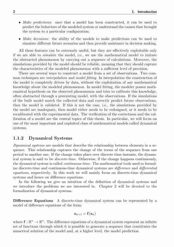
Difference Equations A discrete-time dynamical system can be represented by amodel of difference equations of the form:
xk+1 = f(xk)
where f : Rn → Rn. The difference equations of a dynamical system represent an infiniteset of functions through which it is possible to generate a sequence that constitutes thenumerical solution of the model and, at a higher level, the model prediction.
1.1. Motivations 3
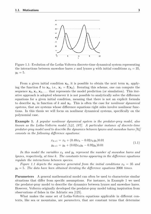
Figure 1.1: Evolution of the Lotka-Volterra discrete-time dynamical system representingthe interactions between snowshoe hares x and lynxes y with initial conditions x0 = 35,y0 = 5.
From a given initial condition x0, it is possible to obtain the next term x1 apply-ing the function f to x0, i.e., x1 = f(x0). Iterating this scheme, one can compute thesequence x0,x1,x2, . . . that represents the model prediction (or simulation). This iter-ative approach is adopted whenever it is not possible to analytically solve the differenceequations for a given initial condition, meaning that there is not an explicit formulato describe xk in function of k and x0. This is often the case for nonlinear dynamicalsystems, that are systems whose difference equations right sides involve nonlinear func-tions. In this thesis we will focus on nonlinear dynamical systems, specifically on thepolynomial case.
Example 1. A popular nonlinear dynamical system is the predator-prey model, alsoknown as the Lotka-Volterra model [142, 187]. A particular instance of discrete-timepredator-pray model used to describe the dynamics between lynxes and snowshoe hares [94]consists in the following difference equations:
xk+1 = xk + (0.48xk − 0.02xkyk)0.01
yk+1 = yk + (0.02xkyk − 0.92yk)0.01(1.1)
In this model the variables xk and yk represent the number of snowshoe hares andlynxes, respectively, at time k. The constants terms appearing in the difference equationsregulate the interactions between species.
Figure 1.1 depicts the sequence generated from the initial conditions x0 = 35 andy0 = 5. The data have been obtained iterating the difference equations 2000 times.
Parameters A general mathematical model can often be used to characterize similarsituations that differ from specific assumptions. For instance, in Example 1 we usedthe predator-pray model to describe the dynamics between lynxes and snowshoe hares.However, Volterra originally developed the predator-pray model taking inspiration fromobservations of fishes in the Adriatic sea [125].
What makes the same set of Lotka-Volterra equations applicable in different con-texts, like sea or mountains, are parameters, that are constant terms that determine
4 1. Introduction
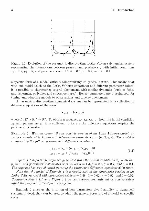
Figure 1.2: Evolution of the parametric discrete-time Lotka-Volterra dynamical systemrepresenting the interactions between prays x and predators y with initial conditionsx0 = 35, y0 = 5, and parameters α = 1.3, β = 0.5, γ = 0.7, and δ = 0.1.
a specific form of a model without compromising its general nature. This means thatwith one model (such as the Lotka-Volterra equations) and different parameter values,it is possible to characterize several phenomena with similar dynamics (such as fishesand fishermen, or lynxes and snowshoe hares). Hence, parameters are a useful tool fortuning and adapting models to observations and diverse phenomena.
A parametric discrete-time dynamical system can be represented by a collection ofdifference equations of the form:
xk+1 = f(xk,p)
where f : Rn×Rm → Rn. To obtain a sequence x0,x1,x2, . . . from the initial conditionx0 and parameters p, it is sufficient to iterate the difference equations keeping theparameter p constant.
Example 2. We now present the parametric version of the Lotka-Volterra model, al-ready encountered in Example 1, introducing parameters p = (α, β, γ, δ). The model iscomposed by the following parametric difference equations:
xk+1 = xk + (αxk − βxkyk)0.01
yk+1 = yk + (δxkyk − γyk)0.01(1.2)
Figure 1.1 depicts the sequence generated from the initial conditions x0 = 35 andy0 = 5, and parameter instantiated with values α = 1.3, β = 0.5, γ = 0.7, and δ = 0.1.The sequence has been obtained iterating the parametric difference equations 2000 times.
Note that the model of Example 1 is a special case of the parametric version of theLotka-Volterra model with parameters set to α = 0.48, β = 0.02, γ = 0.92, and δ = 0.02.Comparing Figure 1.1 with Figure 1.2 we can observe how different parameter valuesaffect the progress of the dynamical system.
Example 2 gives us the intuition of how parameters give flexibility to dynamicalsystems. Indeed, they can be used to adapt the general structure of a model to specificcases.
1.1. Motivations 5
There is a famous quote attributed to John von Neumann by Enrico Fermi [76] thatsummarizes the importance of parameters and the flexibility that their variations cangive to a model: “With four parameters I can fit an elephant, and with five I can makehim wiggle his trunk”.1
1.1.3 Reachability
An interesting problem involving dynamical systems is the verification of their soundnesswith respect to a given specification. Let us imagine that a dynamical system has beenconstructed to study the behavior of a device involved in a safety-critical scenario, i.e, asituation in which a failure of the system may cause serious consequences. In this case,we may want to verify that the modeled device always behaves well and there is no riskin using it.
Several techniques have been developed to study and analyze dynamical systems.Among these, there is formal verification, where it is required to formally establishwhether a dynamical system satisfies a given specification.
An approach to formal verification consists of computing all its possible behaviorsand testing them against the specification. However, it is of usual interest to verifythe model for a uncertain set of initial conditions and parameters (possibly infinite),rather than for single ones. This means that an exhaustive verification procedure maydeal with an infinity of simulations. The problem of computing all the states visitedby a dynamical system is often call reachability problem. Chapter 3 is dedicated to thedefinition and analysis of this problem.
One might suspect that a finite number of simulations is sufficient to verify a dy-namical system, but often there are situations in which small changes in the initialconditions, or in the parameters, cause wild variations in the system behaviors.
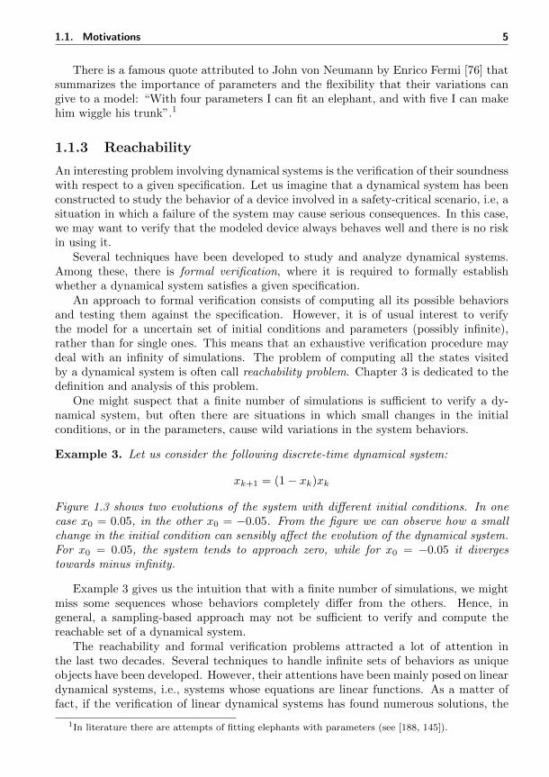
Example 3. Let us consider the following discrete-time dynamical system:
xk+1 = (1− xk)xk
Figure 1.3 shows two evolutions of the system with different initial conditions. In onecase x0 = 0.05, in the other x0 = −0.05. From the figure we can observe how a smallchange in the initial condition can sensibly affect the evolution of the dynamical system.For x0 = 0.05, the system tends to approach zero, while for x0 = −0.05 it divergestowards minus infinity.
Example 3 gives us the intuition that with a finite number of simulations, we mightmiss some sequences whose behaviors completely differ from the others. Hence, ingeneral, a sampling-based approach may not be sufficient to verify and compute thereachable set of a dynamical system.
The reachability and formal verification problems attracted a lot of attention inthe last two decades. Several techniques to handle infinite sets of behaviors as uniqueobjects have been developed. However, their attentions have been mainly posed on lineardynamical systems, i.e., systems whose equations are linear functions. As a matter offact, if the verification of linear dynamical systems has found numerous solutions, the
1In literature there are attempts of fitting elephants with parameters (see [188, 145]).
6 1. Introduction
Figure 1.3: Evolutions with different initial conditions (x0 = 0.05 and x0 = −0.05). Asmall change in the initial condition can affect the evolution of the dynamical system.
analysis of nonlinear dynamical systems remains an open problem that has not yet foundgeneral and efficient solutions. Hence, methods to deal with nonlinear systems, that areparticularly hard to handle, are needed.
Chapter 4 is dedicated to the development of techniques for the computation ofreachable sets of nonlinear (specifically, polynomial) discrete-time dynamical systems.These techniques are useful for the verification of dynamical systems, but they will alsoplay a fundamental role in the identification of valid sets of parameters.
1.1.4 Parameter Synthesis
Parameters play an important role in the versatility of models. The closeness of a modelto the abstracted phenomenon is sensibly influenced by the values of its parameters. It istherefore important to understand how to find good parameter values in order to obtainreliable models. Finding parameters that relate a model with experimental data is afundamental step in model construction that takes the name of parameter estimation.
One major difficulty in parameter estimation is that models may require many pa-rameters, and most of them are neither measurable nor available in literature. Moreover,since often there are many parameter values that can match the observations, param-eter estimation is based not only on the error between the model simulations outputand the observations, but also on the model robustness with respect to parameter varia-tion. From a modeling point of view, robust parameters allow the model to fit new datawithout compromising the fit to the previous ones. This suggests us the importance ofworking with sets of parameters, rather than with single values.
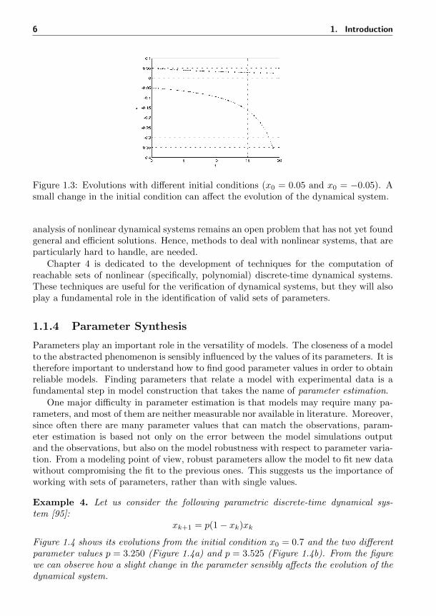
Example 4. Let us consider the following parametric discrete-time dynamical sys-tem [95]:
xk+1 = p(1− xk)xk
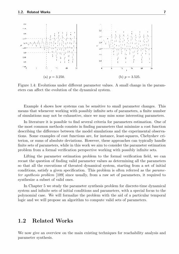
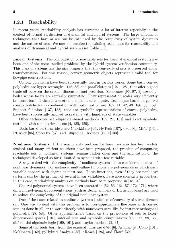
Figure 1.4 shows its evolutions from the initial condition x0 = 0.7 and the two differentparameter values p = 3.250 (Figure 1.4a) and p = 3.525 (Figure 1.4b). From the figurewe can observe how a slight change in the parameter sensibly affects the evolution of thedynamical system.
1.2. Related Works 7
(a) p = 3.250. (b) p = 3.525.
Figure 1.4: Evolutions under different parameter values. A small change in the param-eters can affect the evolution of the dynamical system.
Example 4 shows how systems can be sensitive to small parameter changes. Thismeans that whenever working with possibly infinite sets of parameters, a finite numberof simulations may not be exhaustive, since we may miss some interesting parameters.
In literature it is possible to find several criteria for parameters estimation. One ofthe most common methods consists in finding parameters that minimize a cost functiondescribing the difference between the model simulations and the experimental observa-tions. Some examples of cost functions are, for instance, least-squares, Chebyshev cri-terion, or sums of absolute deviations. However, these approaches can typically handlefinite sets of parameters, while in this work we aim to consider the parameter estimationproblem from a formal verification perspective working with possibly infinite sets.
Lifting the parameter estimation problem to the formal verification field, we canrecast the question of finding valid parameter values as determining all the parametersso that all the executions of threated dynamical system, starting from a set of initialconditions, satisfy a given specification. This problem is often referred as the parame-ter synthesis problem [109] since usually, from a raw set of parameters, it required tosynthesize a subset of valid ones.
In Chapter 5 we study the parameter synthesis problem for discrete-time dynamicalsystem and infinite sets of initial conditions and parameters, with a special focus to thepolynomial case. We will formalize the problem with the aid of a particular temporallogic and we will propose an algorithm to compute valid sets of parameters.
1.2 Related Works
We now give an overview on the main existing techniques for reachability analysis andparameter synthesis.
8 1. Introduction
1.2.1 Reachability
In recent years, reachability analysis has attracted a lot of interest especially in thecontext of formal verification of dynamical and hybrid systems. The large amount oftechniques that have arisen can be cataloged by the complexity of system dynamicsand the nature of sets. We now summarize the existing techniques for reachability andanalysis of dynamical and hybrid system (see Table 1.1).
Linear Systems The computation of reachable sets for linear dynamical systems hasbeen one of the most studied problems by the hybrid system verification community.This class of systems has the nice property that the convexity of sets is preserved undertransformation. For this reason, convex geometric objects represent a valid tool forflowpipe constructions.
Convex polyhedra have been successfully used in various works. Some basic convexpolyhedra are hyper-rectangles [178, 38] and parallelotopes [127, 128], that offer a goodtrade-off between the system dimension and precision. Zonotopes [96, 97, 3] are poly-hedra whose facets are centrally symmetric. Their representation scales very efficientlyin dimension but their intersection is difficult to compute. Techniques based on generalconvex polyhedra in combination with optimization are [107, 41, 42, 43, 186, 85, 169].Support functions [137, 138], that are symbolic representations of convex polyhedra,have been successfully applied to systems with hundreds of state variables.
Other techniques are ellipsoidal-based methods [132, 27, 131] and exact symbolicmethods with semialgebraic sets [4, 135, 159].
Tools based on these ideas are CheckMate [43], HyTech [107], d/dt [6], MPT [134],PHAVer [85], SpaceEx [87], and Ellipsoidal Toolbox (ET) [133].
Nonlinear Systems If the reachability problem for linear systems has been widelystudied and many efficient solutions have been proposed, the problem of computingreachable sets of nonlinear systems remains rather open and the application of thetechniques developed so far is limited to systems with few variables.
A way to deal with the complexity of nonlinear systems, is to consider a subclass ofnonlinear dynamics. For instance, multi-affine functions are polynomials in which eachvariable appears with degree at most one. These functions, even if they are nonlinear(a term can be the product of several linear variables), have nice convexity properties.In this case, reachability analysis on methods have been proposed in [18, 20].
General polynomial systems have been threated in [52, 56, 164, 57, 172, 171], wheredifferent polynomial representations (such as Bezier simplex or Bernstein basis) are usedto reduce the complexity of the original nonlinear system.
One of the issues related to nonlinear systems is the loss of convexity of a transformedset. One way to deal with this problem is to over-approximate flowpipes with convexsets, as done in [9], or to work directly with nonconvex sets, like for instance orthogonalpolyhedra [28, 58]. Other approaches are based on the projections of sets to lower-dimensional spaces [101], interval sets and symbolic computations [165, 77, 88, 36],differential algebraic logic [160, 161], and Taylor models [22, 37].
Some of the tools born from the exposed ideas are d/dt [6], Ariadne [9], Coho [101],KeYmaera [162], pyHybrid Analysis [35], dReach [126], and Flow* [39].
1.2. Related Works 9
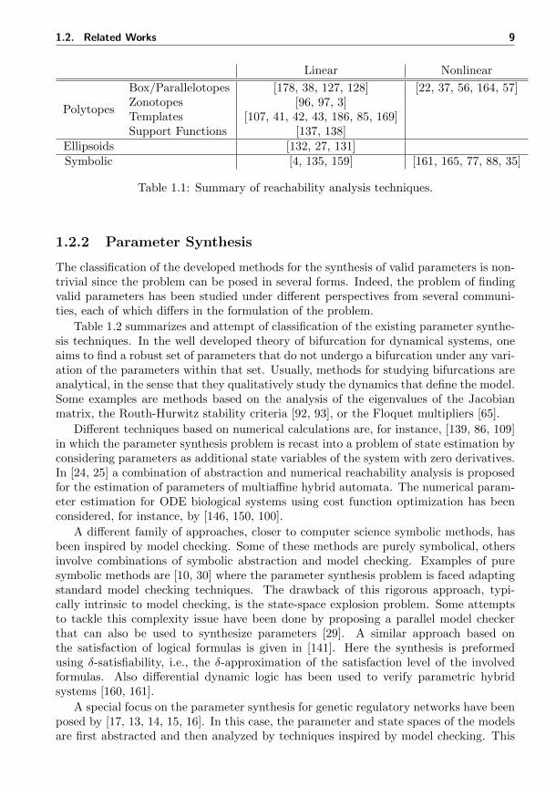
Linear Nonlinear
Polytopes
Box/Parallelotopes [178, 38, 127, 128] [22, 37, 56, 164, 57]Zonotopes [96, 97, 3]Templates [107, 41, 42, 43, 186, 85, 169]Support Functions [137, 138]
Ellipsoids [132, 27, 131]Symbolic [4, 135, 159] [161, 165, 77, 88, 35]
Table 1.1: Summary of reachability analysis techniques.
1.2.2 Parameter Synthesis
The classification of the developed methods for the synthesis of valid parameters is non-trivial since the problem can be posed in several forms. Indeed, the problem of findingvalid parameters has been studied under different perspectives from several communi-ties, each of which differs in the formulation of the problem.
Table 1.2 summarizes and attempt of classification of the existing parameter synthe-sis techniques. In the well developed theory of bifurcation for dynamical systems, oneaims to find a robust set of parameters that do not undergo a bifurcation under any vari-ation of the parameters within that set. Usually, methods for studying bifurcations areanalytical, in the sense that they qualitatively study the dynamics that define the model.Some examples are methods based on the analysis of the eigenvalues of the Jacobianmatrix, the Routh-Hurwitz stability criteria [92, 93], or the Floquet multipliers [65].
Different techniques based on numerical calculations are, for instance, [139, 86, 109]in which the parameter synthesis problem is recast into a problem of state estimation byconsidering parameters as additional state variables of the system with zero derivatives.In [24, 25] a combination of abstraction and numerical reachability analysis is proposedfor the estimation of parameters of multiaffine hybrid automata. The numerical param-eter estimation for ODE biological systems using cost function optimization has beenconsidered, for instance, by [146, 150, 100].
A different family of approaches, closer to computer science symbolic methods, hasbeen inspired by model checking. Some of these methods are purely symbolical, othersinvolve combinations of symbolic abstraction and model checking. Examples of puresymbolic methods are [10, 30] where the parameter synthesis problem is faced adaptingstandard model checking techniques. The drawback of this rigorous approach, typi-cally intrinsic to model checking, is the state-space explosion problem. Some attemptsto tackle this complexity issue have been done by proposing a parallel model checkerthat can also be used to synthesize parameters [29]. A similar approach based onthe satisfaction of logical formulas is given in [141]. Here the synthesis is preformedusing δ-satisfiability, i.e., the δ-approximation of the satisfaction level of the involvedformulas. Also differential dynamic logic has been used to verify parametric hybridsystems [160, 161].
A special focus on the parameter synthesis for genetic regulatory networks have beenposed by [17, 13, 14, 15, 16]. In this case, the parameter and state spaces of the modelsare first abstracted and then analyzed by techniques inspired by model checking. This
10 1. Introduction
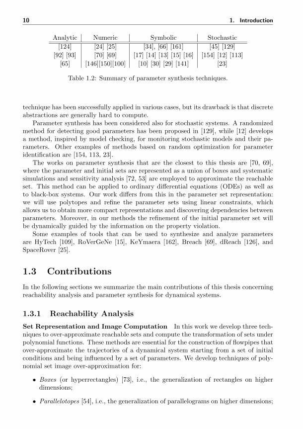
Analytic Numeric Symbolic Stochastic
[124]
[92] [93]
[65]
[24] [25]
[70] [69]
[146][150][100]
[34], [66] [161]
[17] [14] [13] [15] [16]
[10] [30] [29] [141]
[45] [129]
[154] [12] [113]
[23]
Table 1.2: Summary of parameter synthesis techniques.
technique has been successfully applied in various cases, but its drawback is that discreteabstractions are generally hard to compute.
Parameter synthesis has been considered also for stochastic systems. A randomizedmethod for detecting good parameters has been proposed in [129], while [12] developsa method, inspired by model checking, for monitoring stochastic models and their pa-rameters. Other examples of methods based on random optimization for parameteridentification are [154, 113, 23].
The works on parameter synthesis that are the closest to this thesis are [70, 69],where the parameter and initial sets are represented as a union of boxes and systematicsimulations and sensitivity analysis [72, 53] are employed to approximate the reachableset. This method can be applied to ordinary differential equations (ODEs) as well asto black-box systems. Our work differs from this in the parameter set representation:we will use polytopes and refine the parameter sets using linear constraints, whichallows us to obtain more compact representations and discovering dependencies betweenparameters. Moreover, in our methods the refinement of the initial parameter set willbe dynamically guided by the information on the property violation.
Some examples of tools that can be used to synthesize and analyze parametersare HyTech [109], RoVerGeNe [15], KeYmaera [162], Breach [69], dReach [126], andSpaceRover [25].
1.3 Contributions
In the following sections we summarize the main contributions of this thesis concerningreachability analysis and parameter synthesis for dynamical systems.
1.3.1 Reachability Analysis
Set Representation and Image Computation In this work we develop three tech-niques to over-approximate reachable sets and compute the transformation of sets underpolynomial functions. These methods are essential for the construction of flowpipes thatover-approximate the trajectories of a dynamical system starting from a set of initialconditions and being influenced by a set of parameters. We develop techniques of poly-nomial set image over-approximation for:
• Boxes (or hyperrectangles) [73], i.e., the generalization of rectangles on higherdimensions;
• Parallelotopes [54], i.e., the generalization of parallelograms on higher dimensions;
1.3. Contributions 11
• Parallelotope bundles [75], i.e., finite sets of parallelotopes whose intersectionsgenerate polytopes.
The designed techniques share at their cores a property of Bernstein coefficients ofpolynomials. This approach was originally developed in [181, 57] for the reachabilityanalysis of polynomial dynamical systems and boxes. In this work we first extend theoriginal technique to parametric dynamical systems with boxes. Then, we define a newway of approximating and transforming sets using parallelotopes always in combinationwith Bernstein coefficients. This new feature allows one to adopt more flexible sets andobtain finer over-approximating flowpipes. Finally, we further improve the parallelotope-based approximation technique by defining parallelotope bundles, that are sets of paral-lelotopes whose intersections symbolically represent polytopes. We define this new datastructure to represent polytopes and, exploiting the ability of over-approximating the im-ages of single parallelotopes, we define a family of operations for the over-approximationof the images of polytopes. We will exploit parallelotope bundles to define a new reach-ability algorithm for parametric polynomial dynamical systems that produces flowpipesthat are finer than the box-based and parallelotopes-based ones.
Bernstein Coefficients Computation Bernstein coefficients are necessary to ex-press polynomials in Bernstein form [21]. They own several interesting properties [83]including the ability of providing upper and lower bounds of polynomial over the unitbox domain [174]. The techniques developed in this work heavily exploit Bernstein co-efficients. Hence, their computation affects the efficiency and precision of our methods.In this work we contribute to the computation of Bernstein coefficients in several ways:
• We define a new improved matrix method [73] to efficiently compute the Bernsteincoefficients of a given polynomial;
• We introduce the symbolic parametric computation [54] of Bernstein coefficientsto avoid redundant computations;
• We propose a heuristic for subdividing [73] Bernstein coefficients and obtainingtighter bounds of polynomials.
The matrix method [168] is a technique for computing Bernstein coefficients based onoperations on multidimensional matrices that avoids redundant computations. In thiswork we advance the original matrix method defining a more efficient way of transposingmultidimensional matrices. Speeding-up the multidimensional transposition, we boostthe computation of Bernstein coefficients and consequently the flowpipe constructionfor polynomial dynamical systems.
Studying our first reachability algorithm, we noted that we computed similar Bern-stein coefficients for different sets. From certain prospectives, we were wasting com-putations in redundant calculations. For this reason, we developed a new method forsymbolically computing the Bernstein coefficients associated with a particular set thatallows the reachability algorithm to precompute the coefficients only once and then in-stantiate them runtime. This strategy drastically reduces the computational times ofour reachability and parameter synthesis algorithms.
Our final contribution in the context of Bernstein coefficients concerns the precisionof the provided bounds. We developed a subdivision technique to tighten the bounds
12 1. Introduction
and generate finer set image over-approximations based on partial derivatives of thethreated polynomials and the spatial positions of Bernstein coefficients.
1.3.2 Parameter Synthesis
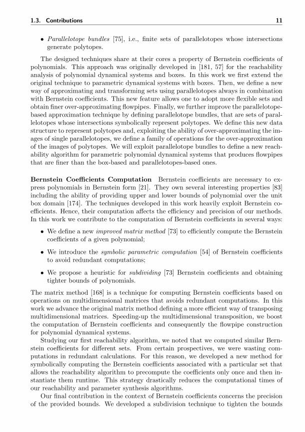
Parameter Synthesis and Signal Temporal Logic Signal Temporal Logic (inshort STL) [143, 144] is a logic suitable for specifying properties of dense-time real-valued signals. In this thesis we adopt STL to formalize the properties that a dynamicalsystem must meet. The contributions of this work that involve parameter synthesis andSTL are:
• The definition of the parameter synthesis problem [55] for dynamical systemsthrough STL specifications;
• The definition of the synthesis semantics [55] for STL formulas;
• The realization of a parameter synthesis algorithm [55] for discrete-time dynamicalsystems and STL properties.
In this thesis we formalize the parameter synthesis problem for dynamical systems withrespect to STL formulas, i.e., given a dynamical system, a set of initial conditions, a setof parameters, and an STL formula, we want to find the largest subset of parameterssuch that all the trajectories of the system starting from the set of initial conditionssatisfy the formula. Since there might be a infinity of trajectories to analyze, we groupthem in a unique flowpipe that over-approximates all the states that a system canreach. However, STL formulas are usually evaluated on single signals, that in thiscase are single trajectories generated by our dynamical system. In order to evaluate aflow of trajectories, we need to adapt the usual semantics of STL. For this reason, wedefine a new semantics, called synthesis semantics, that allows us to reason on flows oftrajectories and whose application to STL formulas produces sets of parameters suchthat the given formulas are satisfied.
We also define a synthesis algorithm that computes the synthesis semantics of anSTL formula for a given discrete-time dynamical system. In particular, our algorithmreceives in input a dynamical system, a set of initial conditions, a set of parameters,and an STL formula. It produces in output a subset of parameters such that all thetrajectories starting from the set of initial conditions satisfy the STL formula. We pro-pose an instance of our algorithm for polynomial discrete-time dynamical systems whosereachable sets can be over-approximated by boxes or parallelotopes, and parameter setscan be represented by polytopes. We prove the correctness and study the computationalcomplexity of our synthesis algorithm.
1.3.3 Tool Implementation
The reachability analysis and parameter synthesis techniques developed in this thesishave been implemented in a C++ tool called Sapo. The main features of our tool arethe following:
• Efficient computation of Bernstein coefficients of polynomials in power basis;
1.4. Structure of the Thesis 13
• Construction of flowpipes that over-approximate reachable sets of polynomial (pos-sibly parametric) discrete-time dynamical systems;
• Synthesis of valid parameter sets with respect to STL specifications for polynomialdiscrete-time dynamical systems.
The computation of Bernstein coefficients is based on our improved matrix method. Theflowpipe construction can be carried out using boxes, parallelotopes, and parallelotopebundles. For the parametric dynamical system, the sets of parameters can be representedas polytopes. The parameter synthesis algorithms supports boxes and parallelotopesto represent sets of states reached by the system and polytopes to represent sets ofparameters.
1.4 Structure of the Thesis
The thesis is structured in the following chapters:
2. Dynamical Systems and Parameters: we begin with the definitions of parametricdynamical system and trajectories. Some illustrative examples are shown to ex-hibit how parameters influence the evolution of systems. We will give an intuitionof what the parameter synthesis problem is and conclude the chapter posing twoimportant questions that are the core of this thesis: how to compute all the statesvisited by a parametric dynamical system in a finite time horizon, and how to findsets of valid parameter values so that a dynamical system behaves well?
3. Parametric Reachability : in this chapter we define and become familiar with theparametric reachability problem, i.e., the problem of determining all the statesvisited by a parametric dynamical system. We will briefly describe the classicalnumerical integration schemes and see how it can be used to compute the trajec-tories generated by dynamical systems. Then, we will focus on the computation ofreachable sets and we will see that the already developed methods can be groupedin two large categories: trajectory-based and set-based techniques. In this work,we will focus on the second one. The chapter ends with a brief discussion aboutthe decidability of the reachability problem;
4. Set Image Computation: in this chapter, with the aim of developing a set-basedreachability algorithm for polynomial dynamical systems, we focus on the problemof computing the polynomial image of a set. As we will discover later, this will bea fundamental task also for the parameter synthesis problem. The chapter startswith the problem formulation and an hypothetical solution based on the polytopicover-approximation of the set. This approach requires the optimization of thetransforming function. Hence, we will introduce Bernstein polynomials whosecoefficients can be used to bound polynomials. We will first adapt the standardBernstein coefficients and their properties to the parametric case, and then we willpresent some new techniques to over-approximate images of sets through boxes,parallelotopes, and parallelotope bundles. We conclude the chapter proposing newmethods to efficiently compute Bernstein coefficients;
14 1. Introduction
5. Parameter Synthesis: this chapter is dedicated to the parameter synthesis prob-lem. In particular, we will give the definition of STL logic and define the newsynthesis semantics that allows us to reason on flows of trajectories and sets ofparameters. Thus, we will formalize the parameter synthesis problem for dynami-cal system through STL specifications. After briefly discussing the decidability ofthe problem, we will present our synthesis algorithm, describing its structure andanalyzing its correctness and computational complexity;
6. Tool and Experimental Results: the developed techniques have been implementedin a tool that is described and evaluated in this chapter. Two main parts composeit: in the first, we will expose the structure of the implemented tool presenting itsmain modules and discussing some implementation choices; in the second, we willapply our tool to some polynomial dynamical systems and evaluate the developedtechniques;
7. Conclusion and Future Works: the thesis ends with some conclusive thoughts anddiscussions on the possible future directions that this work can follow.
2Dynamical Systems and
Parameters
In this chapter we introduce the notion of dynamical systems, important mathematicalobjects widely used to model phenomena evolving in time. The modern theory ofdynamical system dates back to end of the 19th century in the study of the evolution ofthe solar system [31].1 Since then, dynamical systems have found numerous applicationsin important research fields, such as astronomy, biology, physics, and economics.
A dynamical system is often designed to model an observed phenomenon. In order totune the model with the observations, one generally recurs to parameters, i.e., constantterms of the dynamical system that determine a specific form of the system, but notits general nature. Hence, parameters can be used to capture different evolutions of themodeled phenomenon without distorting the dynamical system. However, an importantquestion is: “How to find the values of the parameters in such a way that the dynamicalsystem evolves as expected?”.
This chapter begins with the formalization of dynamical systems, introducing twofundamental classes: the continuous-time dynamical systems (Section 2.1.1) and thediscrete-time dynamical systems (Section 2.1.2). In both cases, we will emphasize therole of parameters. Later, we will introduce the questions that are at the core of thiswork, that are the reachability and the parameter synthesis problems for dynamicalsystems (Section 2.2.1).
A dynamical system is said to be parametric if its dynamics involve parameters, i.e.,constant terms whose values are fixed a priori.
2.1 Dynamical Systems
We begin with some basic notions (some taken from [118]) necessary to define dynamicalsystems.
1It is no surprise that the evolution of a state of a dynamical system is often called orbit.
16 2. Dynamical Systems and Parameters
The state of a system is a description that is sufficient to predict its future. In thiswork we deal with memoryless systems, i.e., systems for which at time t it is possibleto predict the future states without recurring to states prior to t. The space of possiblesystem states is called the state space of the dynamical system.
The nature of a dynamical system is related to the structure of time it relies on.If the time of a system ranges on non-negative real values, then the system is calledcontinuous, while if the time is described by naturals, then the system is said discrete.The evolution of the system over time is a continuous trajectory (in the continuous-timecase) or a sequence (in the discrete-time case) of states through the state space.
The rules that allow us to determine the state of the systems are called dynamics oralso laws of evolution. Typically the dynamics of dynamical systems are described bydifferential equations or difference equations depending on whether they are continuous-time or discrete-time, respectively. Finally, the initial condition is the state at an initialtime from which the evolution starts.
2.1.1 Parametric Continuous-Time Dynamical Systems
Parametric continuous-time dynamical systems are dynamical systems that evolve throughcontinuous time and include parameters in their definition.
Definition 1 (Parametric Continuous-Time Dynamical System). A parametric continuous-time dynamical system is a tuple C = (X ,P, f) where:
• X ⊆ Rn is the state space;
• P ⊆ Rm is the parameter space;
• f : X × P → X is a well-behaving vector field.2
The evolutions of a parametric continuous-time dynamical system are governed bydifferential equations of the form:
x = f(x,p) (2.1)
where x ∈ X are the state variables of the system and p ∈ P are the parameters.The fundamental difference between state variables and parameters is that during theevolution of the dynamical system the values of the state variables can change, whilethe values of the parameters are constant.
For every parameter p ∈ P, if we assume f(x,p) globally Lipschitz continuous inx [140], we guarantee the existence and uniqueness of a solution of the differentialequation x = f(x,p) for every initial condition in X and parameter p ∈ P. Theuniqueness of the solutions ensures that the system is deterministic, i.e., from equalinitial conditions and time lengths, the system evolves identically.
We now formalize the concept of evolution of a dynamical system giving the definitionof trajectory.
Definition 2 (Trajectory of Parametric Continuous-Time Dynamical System). A tra-jectory of a parametric continuous-time dynamical system C = (X ,P, f) starting from
2By well-behaving we mean that the function f has finite derivatives (of all orders) at all points.
2.1. Dynamical Systems 17
a state x ∈ X with parameter p ∈ P is a function ξpx : R≥0 → X such that ξpx is thesolution of the differential equation x = f(x,p) with initial condition x and parameterp, that is:
ξpx (0) = x and ∀t ∈ R≥0, ξpx (t) = f(ξpx (t),p). (2.2)
Let C = (X ,P, f) be a parametric continuous-time dynamical system, X0 ⊆ X bea set of initial conditions, and P ⊆ P be a set of parameters. The set of all possiblecontinuous trajectories of C having initial conditions in X0 and parameters in P is:
Ξ(X0, P ) = ξpx0| x0 ∈ X0,p ∈ P, and ξpx0
is a trajectory of C. (2.3)
Example 5. An example of continuous-time dynamical system is the SIR model [123],often used in biology to model the spread of an epidemic disease.
The SIR model is a dynamical system defined as C = (X ,P, f), with X = R3, P = R2,and f = (fs, fi, fr) such that:
s = fs(s, i, r) = − βsi/Ni = fi(s, i, r) = βsi/N − γir = fr(s, i, r) = γi
(2.4)
The system describes a population of N ∈ R≥0 individuals partitioned in three com-partments: s is the group of susceptible individuals who have not been exposed to thedisease, i is the class of infected individuals, and r are the removed individuals whorecovered from the disease. The migration of individuals from one compartment to an-other is regulated by two parameters: β is the probability for a susceptible individual tobecome infected once there is a contact with an sick person; 1/γ is the mean infectionperiod, that is the time necessary for an infected individual to migrate to the removedcompartment.
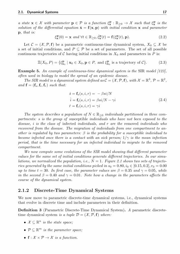
We now compute some evolutions of the SIR model showing that different parametervalues for the same set of initial conditions generate different trajectories. In our simu-lations, we normalized the population, i.e., N = 1. Figure 2.1 shows two sets of trajecto-ries generated by the same initial conditions picked in s0 = 0.80, i0 ∈ [0.15, 0.2], r0 = 0.00up to time t = 30. In first case, the parameter values are β = 0.35 and γ = 0.05, whilein the second β = 0.40 and γ = 0.01. Note how a change in the parameters affects thecourse of the dynamical system.
2.1.2 Discrete-Time Dynamical Systems
We now move to parametric discrete-time dynamical systems, i.e., dynamical systemsthat evolve in discrete time and include parameters in their definition.
Definition 3 (Parametric Discrete-Time Dynamical System). A parametric discrete-time dynamical system is a tuple D = (X ,P, f) where:
• X ⊆ Rn is the state space;
• P ⊆ Rm is the parameter space;
• f : X × P → X is a function.
18 2. Dynamical Systems and Parameters
(a) Evolution of infected individuals i intime.
(b) Evolution of susceptible s, infected i,and removed r individuals in space.
Figure 2.1: Trajectories of continuous-time SIR system with different parameters butsame initial conditions.
The evolutions of parametric discrete-time dynamical systems are governed by dif-ference equation of the form:
xk+1 = f(xk,p) (2.5)
where x ∈ X is the state of the system, p ∈ P are the parameters, and k ∈ N is adiscrete time variable. During the evolution of the dynamical system the state variablescan change their values, while the parameters remain constant. Let us formalize theconcept of evolution through the definition of trajectory.
Definition 4 (Trajectory of Parametric Discrete-Time Dynamical System). A trajec-tory of a parametric discrete-time dynamical system D = (X ,P, f) starting from aninitial state x ∈ X with parameter p ∈ P is a function ξpx : N → X such that ξpx is thesolution of the difference equation xk+1 = f(xk,p) with initial condition x, that is:
ξpx (0) = x and ∀t ∈ N>0, ξpx (t+ 1) = f(ξpx (t),p). (2.6)
Note that differently from the continuous-time systems, a trajectory of a discrete-time system consists in a sequence of states obtainable by iterating the function f .
Let D = (X ,P, f) be a parametric discrete-time dynamical system, X0 ⊆ X be aset of initial conditions, and P ⊆ P be a set of parameters. The set of all possibletrajectories of D with initial conditions in X0 and parameters in P is defined as:
Ξ(X0, P ) = ξpx0| x0 ∈ X0,p ∈ P, and ξpx0
is a trajectory of D. (2.7)
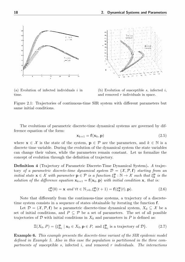
Example 6. This example presents the discrete-time variant of the SIR epidemic modeldefined in Example 5. Also in this case the population is partitioned in the three com-partments of susceptible s, infected i, and removed r individuals. The interactions
2.2. Parameter Synthesis Problem 19
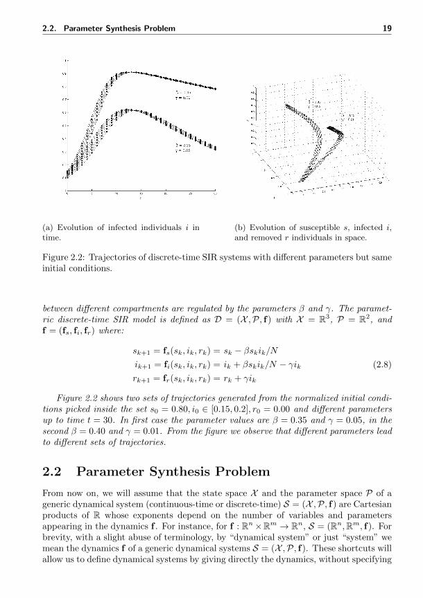
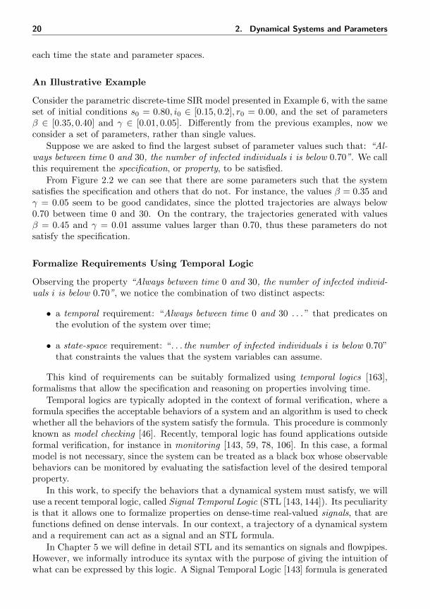
(a) Evolution of infected individuals i intime.
(b) Evolution of susceptible s, infected i,and removed r individuals in space.
Figure 2.2: Trajectories of discrete-time SIR systems with different parameters but sameinitial conditions.
between different compartments are regulated by the parameters β and γ. The paramet-ric discrete-time SIR model is defined as D = (X ,P, f) with X = R3, P = R2, andf = (fs, fi, fr) where:
sk+1 = fs(sk, ik, rk) = sk − βskik/Nik+1 = fi(sk, ik, rk) = ik + βskik/N − γikrk+1 = fr(sk, ik, rk) = rk + γik
(2.8)
Figure 2.2 shows two sets of trajectories generated from the normalized initial condi-tions picked inside the set s0 = 0.80, i0 ∈ [0.15, 0.2], r0 = 0.00 and different parametersup to time t = 30. In first case the parameter values are β = 0.35 and γ = 0.05, in thesecond β = 0.40 and γ = 0.01. From the figure we observe that different parameters leadto different sets of trajectories.
2.2 Parameter Synthesis Problem
From now on, we will assume that the state space X and the parameter space P of ageneric dynamical system (continuous-time or discrete-time) S = (X ,P, f) are Cartesianproducts of R whose exponents depend on the number of variables and parametersappearing in the dynamics f . For instance, for f : Rn×Rm → Rn, S = (Rn,Rm, f). Forbrevity, with a slight abuse of terminology, by “dynamical system” or just “system” wemean the dynamics f of a generic dynamical systems S = (X ,P, f). These shortcuts willallow us to define dynamical systems by giving directly the dynamics, without specifying
20 2. Dynamical Systems and Parameters
each time the state and parameter spaces.
An Illustrative Example
Consider the parametric discrete-time SIR model presented in Example 6, with the sameset of initial conditions s0 = 0.80, i0 ∈ [0.15, 0.2], r0 = 0.00, and the set of parametersβ ∈ [0.35, 0.40] and γ ∈ [0.01, 0.05]. Differently from the previous examples, now weconsider a set of parameters, rather than single values.
Suppose we are asked to find the largest subset of parameter values such that: “Al-ways between time 0 and 30, the number of infected individuals i is below 0.70”. We callthis requirement the specification, or property, to be satisfied.
From Figure 2.2 we can see that there are some parameters such that the systemsatisfies the specification and others that do not. For instance, the values β = 0.35 andγ = 0.05 seem to be good candidates, since the plotted trajectories are always below0.70 between time 0 and 30. On the contrary, the trajectories generated with valuesβ = 0.45 and γ = 0.01 assume values larger than 0.70, thus these parameters do notsatisfy the specification.
Formalize Requirements Using Temporal Logic
Observing the property “Always between time 0 and 30, the number of infected individ-uals i is below 0.70”, we notice the combination of two distinct aspects:
• a temporal requirement: “Always between time 0 and 30 . . . ” that predicates onthe evolution of the system over time;
• a state-space requirement: “. . . the number of infected individuals i is below 0.70”that constraints the values that the system variables can assume.
This kind of requirements can be suitably formalized using temporal logics [163],formalisms that allow the specification and reasoning on properties involving time.
Temporal logics are typically adopted in the context of formal verification, where aformula specifies the acceptable behaviors of a system and an algorithm is used to checkwhether all the behaviors of the system satisfy the formula. This procedure is commonlyknown as model checking [46]. Recently, temporal logic has found applications outsideformal verification, for instance in monitoring [143, 59, 78, 106]. In this case, a formalmodel is not necessary, since the system can be treated as a black box whose observablebehaviors can be monitored by evaluating the satisfaction level of the desired temporalproperty.
In this work, to specify the behaviors that a dynamical system must satisfy, we willuse a recent temporal logic, called Signal Temporal Logic (STL [143, 144]). Its peculiarityis that it allows one to formalize properties on dense-time real-valued signals, that arefunctions defined on dense intervals. In our context, a trajectory of a dynamical systemand a requirement can act as a signal and an STL formula.
In Chapter 5 we will define in detail STL and its semantics on signals and flowpipes.However, we informally introduce its syntax with the purpose of giving the intuition ofwhat can be expressed by this logic. A Signal Temporal Logic [143] formula is generated
2.3. Two Important Questions 21
by the following grammar:
ϕ := s(x1,x2, . . . ,xn) ∼ 0 | ¬ϕ | ϕ ∧ ϕ | ϕUIϕ (2.9)
where s : Rn → R, ∼∈ <,≤, and I is a closed non-singular interval of R≥0. Thereare two elements that distinguish STL from other logics:
• the predicates s(x1,x2, . . . ,xn) ∼ 0 are evaluated on real-values, that in our caseare the states of the dynamical system;
• the temporal operators ϕUIϕ are decorated with intervals that determine the tem-poral windows on which the operators are defined.
From these basic operators, other classical temporal operators can be defined in theusual way, such as true >, false ⊥, eventually/future FIϕ ≡ >UIϕ, or always/globallyGIϕ ≡ ¬FI¬ϕ.
With these elements, we can formalize our requirement expressed in human language“Always between time 0 and 30, the number of infected individuals i is below 0.70” usingthe STL formula G[0,30](i < 0.70).
2.2.1 The Parameter Synthesis Problem
Now that we have defined Signal Temporal Logic formulas, we are ready to formalizethe parameter synthesis problem for a generic dynamical system.
Definition 5 (Parameter Synthesis Problem). Let S = (X ,P, f) be a dynamical system,X0 ⊆ X be a set of initial conditions, P ⊆ P be a set of parameters, and ϕ be an STLspecification. Find the largest subset P ∗ϕ ⊆ P such that:
∀x0 ∈ X0,∀p ∈ P ∗ϕ, ξpx0satisfies ϕ (2.10)
where ξpx0is a trajectory of S.
The notion of formula satisfaction and the parameter synthesis problem will beformalized in Section 5.1.
2.3 Two Important Questions
An intuitive way to generate a valid parameter set is to check the parameters one by oneand populate the set Pϕ. In general, this naive algorithm is incomplete and incorrect.
Incomplete, because the parameter set might be infinite and uncountable, hence wewill never be able to consider all the possible parameter values.
Incorrect, because when we have established the validity of a parameter value, wehave done it considering a finite number of initial conditions and trajectories. If the setof initial conditions is infinite, there might be a point that we have missed such that thecorrespondent trajectory does not satisfy the specification.
These two observations suggest us that in order to solve the parameter synthesisproblem, in the worst case we would need to compute all the trajectories starting fromall the initial conditions with all the parameters. Moreover, even once we have all the
22 2. Dynamical Systems and Parameters
trajectories, we would need to produce a set that contains an infinite number of validparameters. Then, the crucial questions are:
1. How to compute all the parametric trajectories generated from infinite sets ofinitial conditions and parameters?
2. How to compute and represent a valid refinement of the parameter set dealingwith infinite sets?
The objective of this work is to give a possible solution to these questions. InChapter 3 we will clarify the problem of computing all the trajectories generated froman infinite set of initial conditions, while in Chapter 4 we will define some techniquesto over-approximate such computation. Later, in Chapter 5, we will define a method tosynthesize valid parameter sets.
3Parametric Reachability
In this chapter we define and discuss the parametric reachability problem for parametricdynamical systems, i.e., the problem of computing all the states visited by the trajec-tories of a dynamical system starting from a set of initial conditions and being biasedby a set of parameters. This problem plays a central role in the parameter synthesisproblem, since we will be able to determine valid parameter sets only once we are ableto compute the evolution of the system under the influence of the treated parameterset.
The chapter begins with the definition of the reachability problem (Section 3.1), thenit presents the technique of the numerical integration (Section 3.2) and two differentapproaches for the computation of reachable sets (Section 3.3). Finally, there will besome considerations on the decidability of the reachability problem (Section 3.4).
3.1 Parametric Reachability Problem
The problem of computing the states visited by the trajectories of a dynamical systemstarting from an initial set and having a particular parameter set is called the parametricreachability problem.
Let S = (X ,P, f) be a dynamical system. Given two states x,x′ ∈ X , we say that x′
is reachable from x in time 0 ≤ t < +∞ if there are a parameter p ∈ P and a trajectoryξpx of S starting in x such that x′ = ξpx (t). The set of all the states reached by thesystem from x0 ∈ X with parameter p ∈ P is defined as:
Reachp(x0) = x′ | x′ = ξpx0(t), t ∈ T (3.1)
where ξpx0is a trajectory of S and T is the set of non-negative reals R≥0 or the set of
naturals N, depending on whether S is a continuous-time or discrete-time dynamicalsystem, respectively.
We can extend the notion of reachability to sets, that is, given a set of initial condi-tions X0 ⊆ X and a parameter set P ⊆ P, the reachable set is the set of all the states
24 3. Parametric Reachability
reachable by the system:
ReachP (X0) =⋃
x0∈X
⋃p∈P
Reachp(x0). (3.2)
The definition of reachable set reflects the behavior of the dynamical system for aninfinite amount of time. However, we might be interested in studying a model for abounded time horizon. Thus, the set of states reachable in a bounded amount of timeT ∈ T is defined as:
ReachpT (x0) = x′ | x′ = ξpx0(t), 0 ≤ t ≤ T (3.3)
ReachPT (X0) =⋃
x0∈X0
⋃p∈P
ReachpT (x0). (3.4)
Reachable Set Computation
The computation of the reachable set of a dynamical system, in both its bounded orunbounded time versions, might be problematic. The first issue concerns the numericalcomputation of the states visited by a trajectory. With the exception of the caseswhere the trajectories can be characterized by explicit solutions (e.g., x0e
At | t ∈R≥0 for linear systems x = Ax), the usual way to compute the reachable states isto use numerical integration. The second issue interests the possible infinite numberof trajectories we have to deal with, since we might consider infinite sets of initialconditions and parameters. There are several techniques that try to cope with theseproblems. They can be grouped in two classes:
• Trajectory-Based Reachability : a finite number of initial conditions and parame-ters, called nominal values, are chosen. Usually, the nominal values are the resultof a discretization or some statistical assumptions on the state-parameter space.In general, the number of nominal values necessary to reach a certain level ofcoverage of the state-parameter space grows drastically in the dimension of thesystem.
• Set-Based Reachability : considering all the given initial conditions and parame-ters at once, an exhaustive set of trajectories, called flowpipe, is generated. Thisapproach is strongly related to formal verification and set-based computation. Inthis case it is necessary to deal with image computation and manipulation of sets,problems that are mathematically and computationally nontrivial.
In this work we focus exclusively on set-based reachability and on the computationof valid flowpipes for dynamical systems. Before going into the details of our techniques,we become familiar with the notions of numerical integration, trajectory-based and set-based reachability techniques, providing an overview on the existing methods for thereachability problem.
3.2. Numerical Integration 25
3.2 Numerical Integration
Numerical integration is a common technique used to compute the set of states reachableby a dynamical system. The computation of the reachable states (or an approximationof them) is done by simulating1 incrementally the system using discrete-time steps.
The aim of the numerical simulation is to obtain a simulation trace, that is sequenceof states xt0 ,xt1 , . . . , where t0, t1, . . . is a monotonic sequence of time steps and xti ∈ X ,for every ti ∈ N. In order to produce a simulation trace, an integrator needs [110]:
1. an initial value for xt0 ;
2. a procedure to compute xti+1from xti .
A precise integrator will produce a simulation trace xt0 ,xt1 , . . . that is close to theoriginal trajectory generated by the dynamical systems.
Numerical Integration of Continuous-Time Systems
Numerical integration of continuous-time dynamical systems is a well-known and widelystudied mathematical problem for which large collections of techniques have been pro-posed (see, e.g., [61, 130, 110] for surveys on numerical integration or [105, 112] forintegration of ordinary differential equations). The common element among these tech-niques is the discretization scheme that we briefly recall.
Let C = (X ,P, f) be a parametric continuous-time dynamical system. We recall thata valid trajectory ξpx0
of C staring in x0 ∈ X with p ∈ P is such that:
dξpx0(t)
dt= f(ξpx0
(t),p) (3.5)
condition that can be equivalently rewritten as:
ξpx0(t) = x0 +
∫ t
0
f(ξpx0(τ),p)dτ. (3.6)
This suggests us that an approximation xti+1of the state traversed by the trajectory
ξpx0at time ti+1 can be obtained by applying the iterative scheme:
xti+1= xti + gp(xti) (3.7)
where gp is approximation of the integral appearing in Equation 3.6.Some well known examples of numerical integrations are the Euler’s method where:
gp(x) = ∆f(x,p) (3.8)
or the Runge-Kutta’s method :
gp(x) = ∆f(x +∆
2f(x,p),p) (3.9)
1In this work the term simulation is used in the numerical/analytical sense [84] rather than in thealgebraic one [147, 148, 155].
26 3. Parametric Reachability
where ∆ ∈ R is a fixed discretization step. The problem of finding good discretizationfunctions has been widely studied in mathematics and it goes outside the scope of thiswork. For more discretization techniques the reader may refer, e.g., to [61, 130, 110,105, 112].
Numerical Integration of Discrete-Time Systems
The computation of the trajectories of discrete-time systems requires less mechanismsthan the continuous-time case. In fact, here, to obtain a simulation trace xt0 ,xt1 , . . . ,it is sufficient to apply iteratively the system dynamics to an initial condition and aparameter.
Given a parametric discrete-time dynamical systems D = (X ,P, f), the state xti+1
traversed by the trajectory ξpx0at time ti+1 can be obtained by the iterative scheme
dictated by the system dynamics:
xti+1 = f(xti ,p). (3.10)
At the ti-th iteration, the integrator generates a state xti that corresponds exactly tothe state traversed by the trajectory ξpx0
at time ti. Note that here the simulation tracematches exactly the states of the discrete-time trajectory ξpx0
, hence no approximationis introduced by the numerical integration.
In the next sections we will see how numerical integration can be used in differentways to compute the reachable set of a dynamical system. We begin with trajectory-based analysis, where the reachable set is computed in a depth-first fashion. Then, weintroduce set-based analysis, where the reachable set is determined in a breath-first way.We will discuss the benefits and the complications of both the methods, and later wewill focus exclusively on set-based analysis, proposing new techniques to approximatethe reachable set of dynamical systems.
3.3 Reachability Methods
The existing techniques to compute or estimate the reachable sets of dynamical systemscan be grouped in two main categories: trajectory-based and set-based methods.
3.3.1 Trajectory-Based Reachability
Trajectory-based reachability methods are characterized by the depth-first computationof the reachable set (see Figure 3.1). The key steps of these methods are:
1. Selection of an initial condition and parameter;
2. Simulation of the dynamical system up to a maximum time instant (e.g., withsome integration technique like those exposed in Section 3.2);
3. Repetition of Step 1 and 2 until a condition is met.
The halting condition of Step 3 can involve different criteria such as the achieving ofa fix-point in the reachable set computation, the coverage level of the state-parameterspace, or the satisfaction or violation of a specification.

3.3. Reachability Methods 27
Xt0 Xt1 Xt2 Xt3
Figure 3.1: Trajectory-based (black lines) and set-based (gray sets) reachability.
The challenge of this kind of approach resides in the ability of finding conditionsunder which a finite number of simulation is sufficient to deduce all the possible tra-jectories and establish the validity of the system. Such conditions are usually inferredfrom continuity [67, 72] or statistical assumptions of the system under study [190, 26].
The selection of proper initial conditions is usually driven by an abstraction process(often coinciding with partitioning or discretization of the state-parameter space) thatproduces a finite number of quotients of the state-parameter space where each quotientis equivalent with respect to some property. The finite partition is then used to selectsome representative initial conditions and parameters, and construct a flowpipe thatcontains the reachable set [120, 67, 72, 117].
Unluckily there are many cases in which it is not possible to construct a finiteabstraction and it is necessary to recur to approximation techniques. One way is tohalt the abstraction process once it has been reached the level of tolerance expressedby the user. The precision of the result depends on the refinement of the partitions:the finer the partitions, the more accurate the over-approximation of the reachable set.A different approach consists in the relaxation of the definition of equivalence betweenstates [98, 99].
Trajectory-based simulations have found application also outside the scope of reacha-bility analysis. Some examples are the stability analysis of dynamical systems [119, 182],invariant set computation [104, 183] inspired by program analysis [49, 48], i.e., sets fromwhich the system will not escape, and the validation ot falsification of systems againstspecifications [81, 184, 5, 74].
Some tools that exploit trajectory-based methods are Breach [69], S-Taliro [5], andRRT-Rex [74].
3.3.2 Set-Based Reachability
Differently from trajectory-based analysis, set-based reachability methods are character-ized by the incremental computation of the reachable set. The goal here is to computea sequence of sets Xt0 , Xt1 , Xt2 , . . . that constitutes a flowpipe containing all the tra-jectories starting from Xt0 . These methods can be seen as a breath-first computation ofthe reachable set (see Figure 3.1).
The usual way to compute the reachable set of dynamical systems is to use numericalset-integration. Similarly to single trace integrators (see Section 3.2), the key steps a ofa set-based integrator are:
1. Fix a set of initial conditions Xt0 ;
28 3. Parametric Reachability
2. Compute Xti+1 using the set Xti and the parameter set P ;
3. Repeat Step 2 until a condition is met.
Usually the halting condition is defined on a maximum number of steps of the algo-rithm or the achieving of a fix-point in the reachable set computation, checkable by theinclusion Xti+1 ⊆ Xti .
The key element of a set-based method is the computation of the image of a set (seeStep 2). This task is at the core of the exhaustive computation of the transit behaviorof a dynamical system. Nevertheless, the computation of the image of a set can beproblematic and its difficulty depends on the system dynamics and the considered sets.For a survey on the existing reachability techniques see Sections 1.2.1.
3.4 (Un)Decidability
To conclude this overview on the reachability problem, we pose ourselves a fundamentalquestion: Is the reachable set computable? The answer in general is no, since it has beenproved [108] that the reachability problem can be reduced to the halting problem of a2-counter machine (that is undecidable [149]). However, the question as posed, is in itsmost general form. Indeed, there are many variants depending on the considered systemdynamics (linear, nonlinear), sets (polyhedra, ellipsoid, etc.), and time (continuous,discrete, bounded, unbounded).
In this work we focus on polynomial parametric discrete-time dynamical systems, i.e.,parametric discrete-time dynamical systems whose dynamics are polynomials. Thesesystems, in combination with semialgebraic sets (i.e., subsets of Rn defined by a finitesequence of polynomial equations and inequalities, or any finite union of such sets) showinteresting properties. In the next section we will encode the bounded time reachabilityproblem for polynomial discrete-time dynamical systems into the satisfiability of a first-order formula whose decidability is known.
Semialgebraic Reachability
Let D = (X ,P, f) be a polynomial discrete-time dynamical system and X0 ⊆ X , P ⊆ Pbe two semialgebraic sets (note that polytopes fall in this class). We can write twoformulas X0[x] and P [p] that characterize X0 and P , respectively, whose conjunctionXP0[x,p] ≡ X0[x] ∧ P [p] represents the state-parameter space at time zero.
The formula that describes a single step of the system is:
XPi+1[xi+1,p] ≡ ∃xi(XPi[xi,p] ∧ xi+1 = f(xi,p)) (3.11)
that in words means: take xi and p from the state-parameter set XPi[xi,p] , computexi+1 = f(xi,p), and return xi+1 with its correspondent parameter p. Hence, the setreachable in T ∈ N>0 steps can be captured with the formula:
XPT [xT ,p] ≡T∧i=0
∃xi(XPi[xi,p] ∧ xi+1 = f(xi,p)). (3.12)
3.4. (Un)Decidability 29
The set reachable at time T is the set of points that substituted to xT and p make theformula XPT [xT ,p] true. Finding this set is decidable [179] and it can be done by anyquantifier elimination technique [47] (some quantifier elimination tools are QEPCADB [33], Redlog [64], or Z3 [63]).
Example 7. Consider a simple nonlinear dynamical system whose dynamics are xk+1 =f(xk,p) = px2
k, with set of initial conditions X0 = [0.1, 0.2] and parameter set P =[−1.0, 1.0]. The state-parameter set at time zero can be described by the formula:
XP0[x0,p] ≡ 0.1 ≤ x0 ≤ 0.2 ∧ −1.0 ≤ p ≤ 1.0. (3.13)
The set reachable a time 1 can be described by the formula:
XP1[x1,p] ≡ ∃x0(XP0[x0,p] ∧ x1 = f(x0,p))
≡ ∃x0(0.1 ≤ x0 ≤ 0.2 ∧ −1.0 ≤ p ≤ 1.0 ∧ x1 = px20)
(3.14)
whose equivalent version produced by the quantifier eliminator is:
XP1[x1,p] ≡ (−1.0 ≤ p ≤ 1.0 ∧ p + 25x1 = −1)∨(p 6= 0 ∧ px1 ≤ 0 ∧ ((p ≤ 0 ∧ p ≥ −1 ∧ p2 + 25px1 ≥ 0∧p2 + 100px1 ≤ 0) ∨ (p ≥ 0 ∧ p ≤ 1 ∧ p2 + 25px1 ≥ 0∧p2 + 100px1 ≤ 0))).
(3.15)
The drawback of this approach is its computational complexity that is doubly expo-nential in the degree of the formula [102] (or in the number of quantifier alternations,depending on the algorithm). Notice from Example 7 how the degree of the formuladuplicates in a single step. It is not hard to imagine that this approach tends to blowupin time. However, this semialgebraic approach establishes that the exact bounded-timereachability computation for polynomial discrete-time dynamical systems with semial-gebraic sets is decidable.
The next chapter is dedicated to the research of a trade-off between precision andefficiency in the set-image computation problem.

4Set Image Computation
The operation at the core of the reachable set computation is the set image calculation,that is the transformation of a set. This task can be nontrivial, especially when thetransforming function is nonlinear. In this chapter we focus on the problem of computingthe image of sets with respect to polynomial functions. In Section 4.1.2 we will see howthe image set computation can be connected to the problem of optimizing polynomials,issue that will be faced in Section 4.2 through Bernstein coefficients, i.e., coefficients usedto express a polynomial with the Bernstein basis. Bernstein coefficients will be involvedin techniques for over-approximating the transformation of sets using boxes (Section4.3), parallelotopes (Section 4.4), and parallelotope bundles (i.e, sets of parallelotopes)(Section 4.5). At the end of the chapter (Section 4.6), we will focus on the precisionand efficiency of the proposed methods, providing some techniques to obtain tighterover-approximation and faster algorithms.
4.1 Single Step Reachable Set Approximation
The construction of a flowpipe containing the reachable set of a dynamical system isbased on the computation of the image of a set. As previously mentioned, this task canbe difficult, especially when considering nonlinear systems. For instance, such kind ofsystems do not preserve convexity and the generated sets can be hard to handle. It iscommon practice to deal with this issue by over-approximating reachable sets throughconvex sets. The idea is to construct a series of convex sets X0, X1, X2, . . . whose unionleads to a flowpipe that includes all the behaviors of the threated system. The challengeis to efficiently compute an over-approximation that is as tight as possible.
Since we approximate non-convex sets with convex ones, it is very unlikely that wewill obtain the exact reachable set. However, we can try our best, choosing appropriateapproximation sets and squeezing them around the reachable set.
The goal of the next sections is to focus on the computation of a single step reach-ability trying to determine tight sets that over-approximate the states reached by asystem. Formally, given the discrete-time dynamical D = (X ,P, f) and the sets X ⊆ X
32 4. Set Image Computation
and P ⊆ P, we want to find a manipulable tight set X ′ ⊆ X such that:
X ′ ⊇ f(X,P ), (4.1)
where f(X,P ) denotes the set x′ | x′ = f(x,p),x ∈ X,p ∈ P. Note that we do nothave an explicit representation of the set f(x,p) which means that we have to deducethe approximation set X ′ from the previously reached set X, the parameter set P (thatwe assume to be both in an explicit form), and the system dynamics f .
4.1.1 Polytopes
In this section we introduce polytopes, a class of convex sets commonly used in thereachability problem.
Polytopes are the n-dimensional generalization of convex polygons and polyhedra.They are a natural tool to represent sets of states since their facets can be arbitrarilychosen so that precise over-approximations can be obtained.
The term “polytope” is often confusing. Originally, it was introduced by the twelveyears old Alicia Boole Stott (daughter of the logician George Boole) to denote a four-dimensional convex solid [50]. During the years the term has evolved and has been usedto mean related but different mathematical objects.
In geometry a polytope is a geometric object with flat sides definable in any di-mension while the terms polygon and polyhedron denote a two-dimensional and three-dimensional polytope, respectively. However, the terms convex polytope and convexpolyhedra are often used interchangeably. In addition, sometimes polytopes are re-quired to be bounded while others they are allowed to be unbounded.
In this work we use the definition of polytope adopted by the hybrid system com-munity, that is a convex, bounded, with flat sides set of n-dimensional points.
Definition 6 (Polytope). A polytope Q ⊂ Rn is a bounded subset of Rn such that thereis a finite set H = h1, h2, . . . , hm of half-spaces whose intersection is Q, i.e.:
Q =
m⋂i=1
hi, (4.2)
where an half-space h = x | dx ≤ c is a set characterized by a non-null normal vectord ∈ Rn and an offset c ∈ R.
The linear constraints that generate the half-spaces can be organized in a matrixD ∈ Rm×n, called direction matrix (or template) and a vector c ∈ Rk, called offsetvector. The i-th row Di of D together with the i-th component ci of c defines thehalf-space hi ∈ H, being its normal vector and offset, respectively. With a slight abuseof notation, we denote with Q = 〈D, c〉 the polytope generated by the direction matrixD and the offset vector c. Notice that polytopes are bounded subsets of Rn, hence notall the pairs 〈D, c〉 define a polytope.
A polytope Q can be represented as the intersection of different sets of half-spaces.For instance, adding to Q new half-spaces that do not affect the intersection, we get anew representation of Q. Moreover, even without adding new half-spaces we can get anew representation by multiplying the i-th row of D and the i-th component of c by
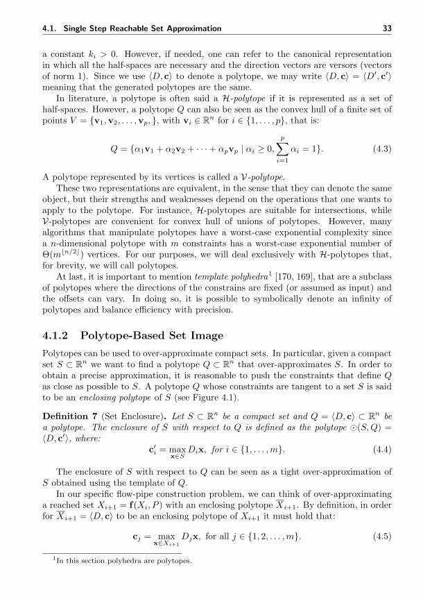
4.1. Single Step Reachable Set Approximation 33
a constant ki > 0. However, if needed, one can refer to the canonical representationin which all the half-spaces are necessary and the direction vectors are versors (vectorsof norm 1). Since we use 〈D, c〉 to denote a polytope, we may write 〈D, c〉 = 〈D′, c′〉meaning that the generated polytopes are the same.
In literature, a polytope is often said a H-polytope if it is represented as a set ofhalf-spaces. However, a polytope Q can also be seen as the convex hull of a finite set ofpoints V = v1,v2, . . . ,vp, , with vi ∈ Rn for i ∈ 1, . . . , p, that is:
Q = α1v1 + α2v2 + · · ·+ αpvp | αi ≥ 0,
p∑i=1
αi = 1. (4.3)
A polytope represented by its vertices is called a V-polytope.These two representations are equivalent, in the sense that they can denote the same
object, but their strengths and weaknesses depend on the operations that one wants toapply to the polytope. For instance, H-polytopes are suitable for intersections, whileV-polytopes are convenient for convex hull of unions of polytopes. However, manyalgorithms that manipulate polytopes have a worst-case exponential complexity sincea n-dimensional polytope with m constraints has a worst-case exponential number ofΘ(mbn/2c) vertices. For our purposes, we will deal exclusively with H-polytopes that,for brevity, we will call polytopes.
At last, it is important to mention template polyhedra1 [170, 169], that are a subclassof polytopes where the directions of the constrains are fixed (or assumed as input) andthe offsets can vary. In doing so, it is possible to symbolically denote an infinity ofpolytopes and balance efficiency with precision.
4.1.2 Polytope-Based Set Image
Polytopes can be used to over-approximate compact sets. In particular, given a compactset S ⊂ Rn we want to find a polytope Q ⊂ Rn that over-approximates S. In order toobtain a precise approximation, it is reasonable to push the constraints that define Qas close as possible to S. A polytope Q whose constraints are tangent to a set S is saidto be an enclosing polytope of S (see Figure 4.1).
Definition 7 (Set Enclosure). Let S ⊂ Rn be a compact set and Q = 〈D, c〉 ⊂ Rn bea polytope. The enclosure of S with respect to Q is defined as the polytope (S,Q) =〈D, c′〉, where:
c′i = maxx∈S
Dix, for i ∈ 1, . . . ,m. (4.4)
The enclosure of S with respect to Q can be seen as a tight over-approximation ofS obtained using the template of Q.
In our specific flow-pipe construction problem, we can think of over-approximatinga reached set Xi+1 = f(Xi, P ) with an enclosing polytope Xi+1. By definition, in orderfor Xi+1 = 〈D, c〉 to be an enclosing polytope of Xi+1 it must hold that:
cj = maxx∈Xi+1
Djx, for all j ∈ 1, 2, . . . ,m. (4.5)
1In this section polyhedra are polytopes.
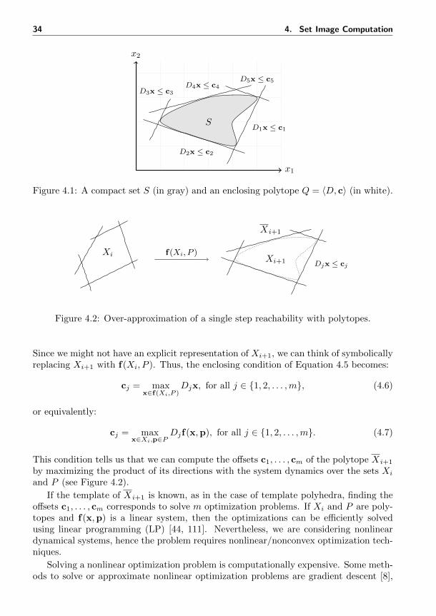
34 4. Set Image Computation
x2
x1
SD1x ≤ c1
D2x ≤ c2
D3x ≤ c3
D5x ≤ c5D4x ≤ c4
Figure 4.1: A compact set S (in gray) and an enclosing polytope Q = 〈D, c〉 (in white).
Xi f(Xi, P )Xi+1
Xi+1
Djx ≤ cj
Figure 4.2: Over-approximation of a single step reachability with polytopes.
Since we might not have an explicit representation of Xi+1, we can think of symbolicallyreplacing Xi+1 with f(Xi, P ). Thus, the enclosing condition of Equation 4.5 becomes:
cj = maxx∈f(Xi,P )
Djx, for all j ∈ 1, 2, . . . ,m, (4.6)
or equivalently:
cj = maxx∈Xi,p∈P
Djf(x,p), for all j ∈ 1, 2, . . . ,m. (4.7)
This condition tells us that we can compute the offsets c1, . . . , cm of the polytope Xi+1
by maximizing the product of its directions with the system dynamics over the sets Xi
and P (see Figure 4.2).
If the template of Xi+1 is known, as in the case of template polyhedra, finding theoffsets c1, . . . , cm corresponds to solve m optimization problems. If Xi and P are poly-topes and f(x,p) is a linear system, then the optimizations can be efficiently solvedusing linear programming (LP) [44, 111]. Nevertheless, we are considering nonlineardynamical systems, hence the problem requires nonlinear/nonconvex optimization tech-niques.
Solving a nonlinear optimization problem is computationally expensive. Some meth-ods to solve or approximate nonlinear optimization problems are gradient descent [8],
4.2. Bounding Polynomials 35
interior point method [60, 121], or sum of squares techniques [158, 157]. Unluckily, theirscalability in the number of variables, degree of the function to optimize, and numberof constraints, is not sufficiently efficient for our verification purposes.
A way to face the non linearity issue is to relax the enclosing constraints of the facetsof Xi+1, namely, instead or requiring the facets to be tangent to reached set, we try topush them as close as possible without falling in the complexity trap. Mathematicallyspeaking, instead of finding the optimum cj of Equation 4.7, we try to efficiently lookfor upper bounds cj ≥ cj such that:
cj ≥ cj = maxx∈Xi,p∈P
Djf(x,p), for all j ∈ 1, 2, . . . ,m. (4.8)
The result will be a polytope Xi+1 = 〈D, c〉 which might not be an enclosing for Xi+1,but will over-approximate the reached set. The quality of the approximation dependson how close the upper bounds cj are to the optimums cj .
4.2 Bounding Polynomials
In the previous section we have seen how the optimization of a function can be usedto over-approximate the image of a set and thus compute the flowpipe of a dynamicalsystem. In this section we focus on the problem of optimizing a polynomial over somesubclasses of polytopes. The presented technique is based on the Bernstein expansionof polynomials and their properties, a mathematical tool that we will often use in thiswork.
A Bernstein polynomial is a polynomial expressed in the Bernstein form, that is alinear combination of the Bernstein basis polynomials. As we will see in the following, thecoefficients associated with these basis own interesting properties that can be exploitedto bound the image of a polynomial over a unit box domain.
This section is organized in two parts. First, we introduce Bernstein basis and theirproperties in their original form considering polynomials of the form π(x) : Rn → R.Second, we extend the definition of Bernstein expansion to parametric polynomials ofthe kind π(x,p) : Rn × Rm → R. We will demonstrate that important propertiesof standard Bernstein basis also hold in the parametric case. These proofs will be thekey element for bounding parametric polynomials, computing parametric flowpipes, andlater, synthesizing valid parameter sets.
4.2.1 Bernstein Basis and Coefficients
Before defining the Bernstein basis, we introduce some notations useful to work withpolynomials.
A multi-index is a vector i = (i1, i2, . . . , in) where each ij ∈ N. Given two multi-indices i and d of the same dimension, we write i ≤ d (d dominates i) if for all j ∈1, 2, . . . , n, ij ≤ dj . Also, we write i/d for the multi-index (i1/d1, i2/d2, . . . , in/dn)
and
(d
i
)for the product of the binomial coefficients
(d1
i1
)(d2
i2
). . .
(dnin
).
36 4. Set Image Computation
A polynomial π(x) : Rn → R can be represented using the power basis as follows:
π(x) =∑i∈Iπ
aixi (4.9)
where i = (i1, i2, . . . , in) is a multi-index of size n ∈ N and xi denotes the monomialxi11 xi2
2 . . .xinn . The set Iπ is called the multi-index set of π. The degree d of π is the
smallest multi-index that dominates all the multi-indices of Iπ, i.e., for all i ∈ Iπ, i ≤ d.The coefficients ai ∈ R assume real values.
Example 8. Consider the polynomial π(x1,x2) = 1/3x21−1/2x2 + 1/4x1x2 + 1/2. The
multi-index set of π is Iπ = (2, 0), (0, 1), (1, 1), (0, 0) and the associated coefficientsare a(2,0) = 1/3,a(0,1) = −1/2,a(1,1) = 1/4, and a(0,0) = 1/2.
Bernstein basis polynomials of degree d are basis for the space of polynomials ofdegree at most d over Rn. For x = (x1,x2, . . . ,xn) ∈ Rn, the i-th Bernstein polynomialof degree d is defined as:
B(d,i)(x) = βd1,i1(x1)βd2,i2(x2) . . . βdn,in(xn) (4.10)
where, for a real number x ∈ R,
βdj ,ij (x) =
(djij
)xij (1− x)dj−ij . (4.11)
A polynomial π(x) : Rn → R can be represented using Bernstein basis as:
π(x) =∑i∈Iπ
biB(d,i)(x) (4.12)
where, for each i ∈ Iπ, the Bernstein coefficient, is defined as:
bi =∑j≤i
(ij
)(dj
)aj. (4.13)
Notice how Bernstein coefficients can be calculated from the coefficients of the mono-mials of the threated polynomial in power basis. The (n + 1)-dimensional points(i/d,bi) ∈ Rn+1 are called Bernstein control points.
Example 9. Consider the polynomial π(x1,x2) = 1/3x21− 1/2x2 + 1/4x1x2 + 1/2 from
Example 8. For illustrative purposes, we examine only the multi-indices (1, 1) whosecorrespondent Bernstein coefficient is:
b(1,1) =
((1,1)(1,1)
)((2,1)(1,1)
)1/4−
((1,1)(0,1)
)((2,1)(0,1)
)1/2 +
((1,1)(1,0)
)((2,1)(1,0)
)0 +
((1,1)(0,0)
)((2,1)(0,0)
)1/2 = 0.125. (4.14)
Applying the same scheme to the other multi-indices, we obtain the Bernstein coefficientsb(0,0) = 0.5, b(0,1) = 0.0, b(1,0) = 0.5, b(1,1) = 0.125, b(2,0) = 0.834, and b(2,1) = 0.584.
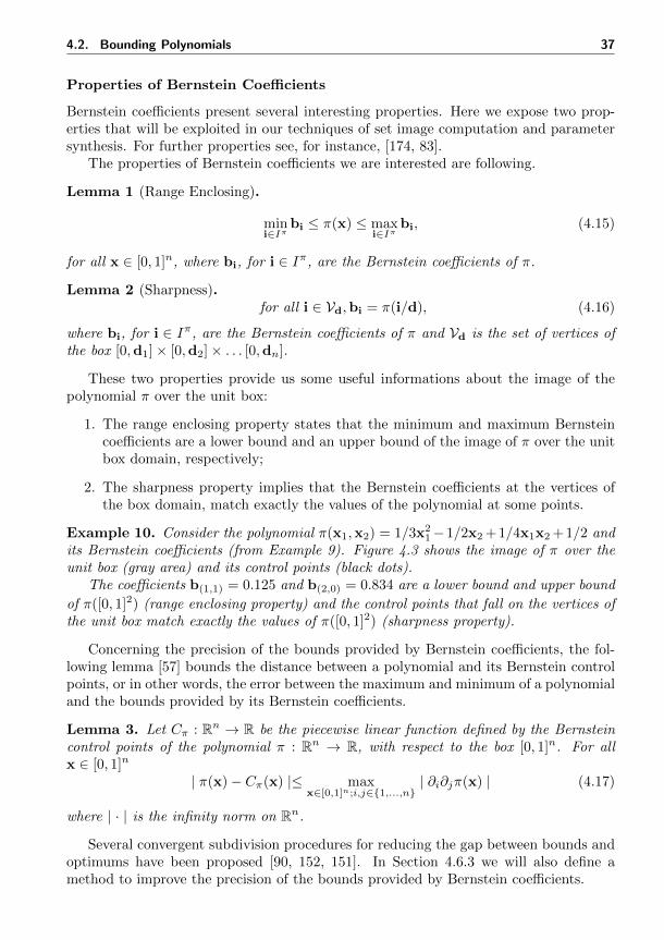
4.2. Bounding Polynomials 37
Properties of Bernstein Coefficients
Bernstein coefficients present several interesting properties. Here we expose two prop-erties that will be exploited in our techniques of set image computation and parametersynthesis. For further properties see, for instance, [174, 83].
The properties of Bernstein coefficients we are interested are following.
Lemma 1 (Range Enclosing).
mini∈Iπ
bi ≤ π(x) ≤ maxi∈Iπ
bi, (4.15)
for all x ∈ [0, 1]n, where bi, for i ∈ Iπ, are the Bernstein coefficients of π.
Lemma 2 (Sharpness).for all i ∈ Vd,bi = π(i/d), (4.16)
where bi, for i ∈ Iπ, are the Bernstein coefficients of π and Vd is the set of vertices ofthe box [0,d1]× [0,d2]× . . . [0,dn].
These two properties provide us some useful informations about the image of thepolynomial π over the unit box:
1. The range enclosing property states that the minimum and maximum Bernsteincoefficients are a lower bound and an upper bound of the image of π over the unitbox domain, respectively;
2. The sharpness property implies that the Bernstein coefficients at the vertices ofthe box domain, match exactly the values of the polynomial at some points.
Example 10. Consider the polynomial π(x1,x2) = 1/3x21−1/2x2 +1/4x1x2 +1/2 and
its Bernstein coefficients (from Example 9). Figure 4.3 shows the image of π over theunit box (gray area) and its control points (black dots).
The coefficients b(1,1) = 0.125 and b(2,0) = 0.834 are a lower bound and upper bound
of π([0, 1]2) (range enclosing property) and the control points that fall on the vertices ofthe unit box match exactly the values of π([0, 1]2) (sharpness property).
Concerning the precision of the bounds provided by Bernstein coefficients, the fol-lowing lemma [57] bounds the distance between a polynomial and its Bernstein controlpoints, or in other words, the error between the maximum and minimum of a polynomialand the bounds provided by its Bernstein coefficients.
Lemma 3. Let Cπ : Rn → R be the piecewise linear function defined by the Bernsteincontrol points of the polynomial π : Rn → R, with respect to the box [0, 1]n. For allx ∈ [0, 1]n
| π(x)− Cπ(x) |≤ maxx∈[0,1]n;i,j∈1,...,n
| ∂i∂jπ(x) | (4.17)
where | · | is the infinity norm on Rn.
Several convergent subdivision procedures for reducing the gap between bounds andoptimums have been proposed [90, 152, 151]. In Section 4.6.3 we will also define amethod to improve the precision of the bounds provided by Bernstein coefficients.
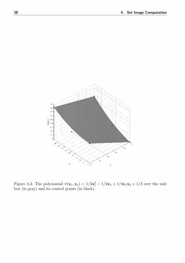
38 4. Set Image Computation
Figure 4.3: The polynomial π(x1,x2) = 1/3x21 − 1/2x2 + 1/4x1x2 + 1/2 over the unit
box (in gray) and its control points (in black).
4.2. Bounding Polynomials 39
4.2.2 Parametric Bernstein Basis and Coefficients
Bernstein coefficients and their properties are useful tools for bounding polynomials.However, since we work with parametric dynamical systems, we want to bound para-metric polynomials of the kind π(x,p) : Rn × Rm → R. Thus, we have to extend thedefinition of Bernstein basis to the parametric case. We will see that all the presentedproperties related to the Bernstein coefficients also hold when parameters are involved.
A parametric polynomial π(x,p) : Rn × Rm → R can be represented in the powerbasis as:
π(x,p) =∑i∈Iπ
ai(p)xi, (4.18)
where the coefficients ai(p) : Rm → R, for i ∈ Iπ, are functions defined over theparameters p ∈ Rm.
Example 11. Consider the parametric polynomial π(x1,x2,p1) = 1/3p1x21−1/2p1x2+
1/4x1x2+1/2. The parametric coefficients are a(2,0)(p1) = 1/3p1, a(0,1)(p1) = −1/2p1,a(1,1)(p1) = 1/4, and a(0,0)(p1) = 1/2.
A parametric polynomial π(x,p) : Rn×Rm → R can be represented using Bernsteinbasis as:
π(x,p) =∑i∈Iπ
bi(p)B(d,i)(x) (4.19)
where, for each i ∈ Iπ, the parametric Bernstein coefficient, is defined as:
bi(p) =∑j≤i
(ij
)(dj
)aj(p). (4.20)
Differently from the nonparametric case, the parametric Bernstein coefficients are func-tions of the form bi(p) : Rm → R.
Example 12. Consider the polynomial π(x1,x2,p1) = 1/3p1x21−1/2p1x2 +1/4x1x2 +
1/2 from Example 11. For illustrative purposes, we study only the multi-index (1, 1)whose parametric Bernstein coefficient is:
b(1,1)(p1) =
((1,1)(1,1)
)((2,1)(1,1)
)1/4−
((1,1)(0,1)
)((2,1)(0,1)
)1/2p1 +
((1,1)(1,0)
)((2,1)(1,0)
)0 +
((1,1)(0,0)
)((2,1)(0,0)
)1/2 = 0.625− 0.5p1. (4.21)
Applying the same scheme to the other multi-indices, we obtain the parametric Bernsteincoefficients b(0,0)(p1) = 0.5, b(0,1)(p1) = 0.5 − 0.5p1, b(1,0)(p1) = 0.5, b(1,1)(p1) =0.625− 0.5p1, b(2,0)(p1) = 0.334p1 + 0.5, and b(2,1)(p1) = 0.75− 0.1667p1.
Properties of Parametric Bernstein Coefficients
We now extend range enclosing and sharpness properties defined on polynomials (seeSection 4.2.1) to the parametric case. Let P ⊂ Rm be a polytope.
40 4. Set Image Computation
Lemma 4 (Parametric Range Enclosing).
mini∈Iπ
minp∈P
bi(p) ≤ π(x,p) ≤ maxi∈Iπ
maxp∈P
bi(p), (4.22)
for all x ∈ [0, 1]n and p ∈ P , where bi(p), for i ∈ Iπ, are the parametric Bernsteincoefficients of π.
Lemma 5 (Parametric Sharpness).
for all i ∈ Vd and p ∈ P,bi(p) = π(i/d,p), (4.23)
where bi(p), for i ∈ Iπ, are the parametric Bernstein coefficients of π and Vd is the setof vertices of the box [0,d1]× [0,d2]× . . . [0,dn].
Proof. Both Lemma 4 and Lemma 5 directly follow from Lemma 1 and 2, respectively.In fact any instantiation of the parametric case holds by the standard properties ofBernstein coefficients (see Lemmas 1 and 2). This is true for every parameter valuep ∈ P , which implies the validity of Lemma 4 and Lemma 5.
Similarly to the standard Bernstein coefficients properties, the parametric coefficientscan be used to get information about the evaluation of a parametric polynomial π(x,p)over the unit box under the influence of the parameters p ∈ P . Precisely:
1. The parametric range enclosing property can be used to find lower bound andupper bound;
2. The parametric sharpness property tells us where a parametric control pointmatches exactly the value of the parametric polynomial π(x,p).
Example 13. Consider the polynomial π(x1,x2,p1) = 1/3p1x21−1/2p1x2 +1/4x1x2 +
1/2, its Bernstein coefficients (from Example 12), and the parameter set P = [−0.1, 0.1].Figure 4.4 shows two images of π over the unit box and parameter p1 with values −0.1and 0.1 (gray areas), and the parametric control points ranging over the parameter setP = [−0.1, 0.1] (in black). Also in this case, it is possible to see how the parametricrange enclosing and sharpness properties hold.
4.2.3 Computation of upper bound and lower bound
The parametric range enclosing property can be used to determine an upper and lowerbound of a parametric polynomial π(x,p) : Rn×Rm → R with x ∈ [0, 1]n and p ∈ P ⊂Rm polytope. We now define the algorithm maxBernCoeff (see Algorithm 1) that,exploiting Bernstein coefficients, determines an upper bound of a polynomial over theunit box and a polytopic parameter set.
maxBernCoeff begins by computing the set Bπ of all the parametric Bernsteincoefficients of the polynomial π(x,p). This can be done using Equation 4.20. Thus, foreach coefficient bi(p) ∈ Bπ, the algorithm maximizes bi(p) over the parameter set Pand updates the current maximum b. Note that if bi(p) is linear in p, the optimizationover P can be carried out using linear programming. At the end of the loop, b will bean upper bound on the polynomial π(x,p) over the unit box and parameter set P .
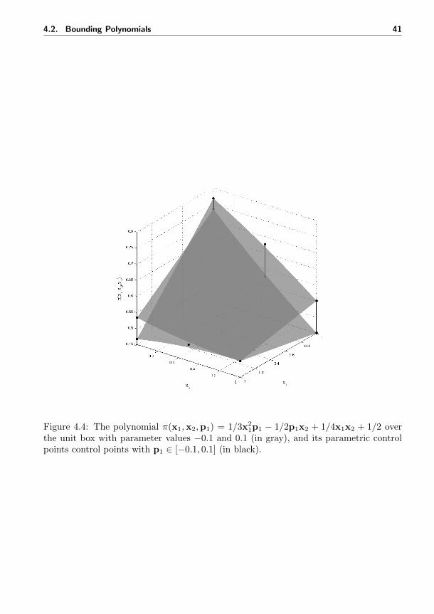
4.2. Bounding Polynomials 41
Figure 4.4: The polynomial π(x1,x2,p1) = 1/3x21p1 − 1/2p1x2 + 1/4x1x2 + 1/2 over
the unit box with parameter values −0.1 and 0.1 (in gray), and its parametric controlpoints control points with p1 ∈ [−0.1, 0.1] (in black).
42 4. Set Image Computation
Algorithm 1 Compute maximum parametric Bernstein Coefficient
1: function maxBernCoeff(π, P ) . π(x,p) : Rn × Rm → R, P ⊂ Rm polytope2: Bπ ←BernCoeffs(π) . Compute Bernstein coefficients3: b← −∞ . Initialize current maximum4: for bi(p) ∈ Bπ do5: b← max
p∈Pbi(p) . Maximize current coefficient
6: b← maxb, b . Update maximum7: end for8: return b9: end function
Similarly, we can define the algorithm minBernCoeff that computes a lower boundof π(x,p). minBernCoeff can be easily obtained from maxBernCoeff by initializingthe bound b with +∞ (Line 3) and replacing maximum operators with minimums.
4.2.4 Summary
Bernstein coefficients can be used to bound the image of a polynomial, eventually para-metric, over the unit box. However, it is very unlikely that the trajectories generated bya dynamical system will only span over unit boxes. The question is then how to exploitBernstein coefficients outside unit boxes and perhaps outside box domains.
In the next chapters, we will define some techniques of set image approximation thatinvolve generic boxes, parallelotopes, and sets generated by the intersection of severalparallelotopes. These techniques will be used to compute over-approximations of sets ofstates reached by polynomial dynamical systems and will allow us to synthesize sets ofparameters so that all the trajectories of the treated dynamical system satisfy a givenSTL property.
Moreover, at the end of the chapter, we will present some techniques to improve theefficiency with which Bernstein coefficients are computed and to obtain tighter bounds.These improvements will lead to faster and preciser reachability and parameter synthesisalgorithms.
4.3 Boxes
We now go into the problem of the image computation. We begin by considering one ofsimplest class of sets called boxes, also known as hyper-rectangles.
Definition 8 (Box). A set B ⊂ Rn is a box if and only if it can be expressed as theproduct of n intervals, that is:
B = [x1, x1]× . . . [xn, xn] =
n∏i=1
[xi, xi], (4.24)
where xi, xi ∈ R, for i ∈ 1, . . . , n.
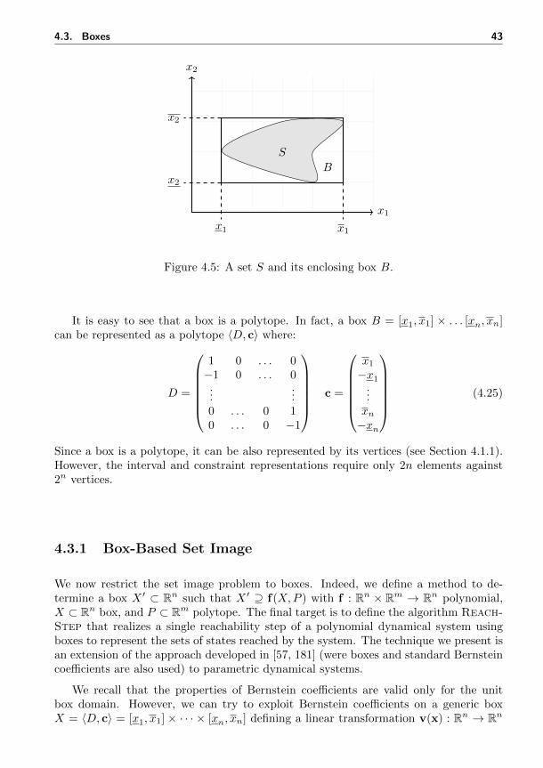
4.3. Boxes 43
x2
x1x1 x1
x2
x2
S
B
Figure 4.5: A set S and its enclosing box B.
It is easy to see that a box is a polytope. In fact, a box B = [x1, x1] × . . . [xn, xn]can be represented as a polytope 〈D, c〉 where:
D =
1 0 . . . 0−1 0 . . . 0...
...0 . . . 0 10 . . . 0 −1
c =
x1−x1
...xn−xn
(4.25)
Since a box is a polytope, it can be also represented by its vertices (see Section 4.1.1).However, the interval and constraint representations require only 2n elements against2n vertices.
4.3.1 Box-Based Set Image
We now restrict the set image problem to boxes. Indeed, we define a method to de-termine a box X ′ ⊂ Rn such that X ′ ⊇ f(X,P ) with f : Rn × Rm → Rn polynomial,X ⊂ Rn box, and P ⊂ Rm polytope. The final target is to define the algorithm Reach-Step that realizes a single reachability step of a polynomial dynamical system usingboxes to represent the sets of states reached by the system. The technique we present isan extension of the approach developed in [57, 181] (were boxes and standard Bernsteincoefficients are also used) to parametric dynamical systems.
We recall that the properties of Bernstein coefficients are valid only for the unitbox domain. However, we can try to exploit Bernstein coefficients on a generic boxX = 〈D, c〉 = [x1, x1] × · · · × [xn, xn] defining a linear transformation v(x) : Rn → Rn
44 4. Set Image Computation
that maps the unit box to X. The map v(x) is defined as follows:
v(x) =
x1 − x1 0 . . . 0
0 x2 − x2 . . . 0...
...0 . . . 0 xn − xn
x1
x2
...xn
+
x1x2...xn
. (4.26)
Now, suppose we want to bound a parametric polynomial π : Rn×Rm → R over a boxX ⊂ Rn and a polytopic parameter set P ⊂ Rm. We can compute the map v(x) for Xand then consider the composition π(v(x),p). It holds that π(X,P ) = π(v([0, 1]n), P ).Note that the domain of π(v(x),p) in x is the unit box. This means that we can use theBernstein coefficients of π(v(x),p), and in particular the algorithm maxBernCoeff(see Algorithm 1), to indirectly bound π(x,p) over X and P .
We can define the function bound (Algorithm 2) that receives in input a parametricpolynomial π : Rn × Rm → R, a box X ⊂ Rn, and a polytopic parameter set P ⊂ Rm.Exploiting the map v(x) and Bernstein coefficients, it returns an upper bound b ∈ R ofπ(X,P ) such that:
b ≥ maxx∈[0,1]n,p∈P
π(v(x),p) = maxx∈X,p∈P
π(x,p). (4.27)
Algorithm 2 Bound polynomial over box and polytopic parameter set
1: function bound(π,X, P ) . X ⊂ Rn box, P ⊂ Rm polytope2: v(x)←mapUnitBoxTo(X) . Map [0, 1]n to X3: b←maxBernCoeff(π(v(x)), P ) . Compute maximum coefficient4: return b5: end function
The function bound, using the function mapUnitBoxTo based on Equation 4.26,computes the transformation v(x) (Line 2) that maps the unit box to the given box X.Then, through the function maxBernCoeff, it computes the Bernstein coefficients ofπ(v(x),p) and returns their maximum over the parameter set P (Line 3).
Now that we know how to bound a polynomial over a generic box, we can focus on theimage set computation. Let f : Rn×Rm → Rn be a parametric polynomial, X,X ′ ⊂ Rnbe boxes, and P ⊂ Rm be a polytopic parameter set. In order for X ′ = 〈D, c′〉 to be anover-approximation box of the set f(X,P ) it must hold that:
c′j ≥ maxx∈X,p∈P
Djf(x,p) for all j ∈ 1, . . . , 2n. (4.28)
Since the functions Djf(x,p) are polynomials and X ⊂ Rn and P ⊂ Rm are a boxand a polytope, respectively, the upper bounds c′j , for j ∈ 1, . . . , 2n, can obtainedexploiting the algorithm bound. The optimizations of the functions Djf(x,p) lead tothe offsets c′j that associated with the template D generate the over-approximation boxX ′ = 〈D, c′〉 ⊇ f(X,P ).
We collect these operations in the algorithm reachStep (Algorithm 3) that receives
4.3. Boxes 45
in input a box X ⊂ Rn and a polytope P ⊂ Rm, and, exploiting the algorithm bound,computes a box X ′ that over-approximates the image f(X,P ).
Algorithm 3 Box-based reachability step
1: function reachStep(X,P ) . X = 〈D, c〉 ⊂ Rn box, P ⊂ Rm polytope2: for i ∈ 1, . . . , 2n do3: c′i ←bound(Dif(x,p), X, P ) . Bound box directions4: end for5: return X ′ = 〈D, c′〉 . Construct and return the new box6: end function
Example 14. Consider the dynamics of the discrete-time SIR epidemic system of Ex-ample 6 with state variables and parameters grouped in the vectors x = (s, i, r) andp = (β, γ):
f(x,p) =
fs(x,p) = s− βsifi(x,p) = i+ βsi− γifr(x,p) = r + γi
(4.29)
Let s ∈ [0.80, 0.85], i ∈ [0.15, 0.20], r ∈ [0, 0], and β ∈ [0.35, 0.36], γ ∈ [0.05, 0.06]whose box-set representations are X = 〈D, c〉 = [0.80, 0.85] × [0.15, 0.20] × [0, 0] andP = [0.35, 0.36]× [0.05, 0.06].
The map v that transforms the unit box to X is:
v(x) =
0.85− 0.80 0 00 0.20− 0.15 00 0 0− 0
sir
+
0.800.15
0
(4.30)
whose composition with the system dynamics leads to the function:
h(x,p) =
fs(v(x),p) = (0.05s+ 0.80)− β(0.05s+ 0.80)(0.05i+ 0.15)fi(v(x),p) = (1− γ)(0.05i+ 0.15) + β(0.05s+ 0.80)(0.05i+ 0.15)fr(v(x),p) = γ(0.05i+ 0.15)
(4.31)
Composing the function h(x,p) with the box template D, we obtain the functions:
D1h(x,p) = (0.05s+ 0.80)− β(0.05s+ 0.80)(0.05i+ 0.15)
D2h(x,p) = − (0.05s+ 0.80) + β(0.05s+ 0.80)(0.05i+ 0.15)
D3h(x,p) = (1− γ)(0.05i+ 0.15) + β(0.05s+ 0.80)(0.05i+ 0.15)
D4h(x,p) = − (1− γ)(0.05i+ 0.15)− β(0.05s+ 0.80)(0.05i+ 0.15)
D5h(x,p) = γ(0.05i+ 0.15)
D6h(x,p) = − γ(0.05i+ 0.15)
(4.32)
46 4. Set Image Computation
whose Bernstein coefficients are:
BD1h(p) = 0.80− 0.12β, 0.80− 0.16β, 0.85− 0.13β, 0.85− 0.17βBD2h(p) = 0.12β − 0.80, 0.16β − 0.80, 0.13β − 0.85, 0.17β − 0.85BD3h(p) = 0.12β − 0.15γ + 0.15, 0.16β − 0.20γ + 0.20,
0.13β − 0.15γ + 0.15, 0.17β − 0.20γ + 0.20BD4h(p) = 0.15γ − 0.12β − 0.15, 0.20γ − 0.16β − 0.20,
0.15γ − 0.13β − 0.15, 0.20γ − 0.17β − 0.20BD5h(p) = 0.15γ, 0.2γBD6h(p) = −0.15γ,−0.2γ
(4.33)
that optimized on the parameter set P lead to the upper bounds:
0.8054 = maxp∈Pbi(p) ∈ BD1h(p) − 0.7424 = max
p∈Pbi(p) ∈ BD2h(p)
0.2512 = maxp∈Pbi(p) ∈ BD3h(p) − 0.1830 = max
p∈Pbi(p) ∈ BD4h(p)
0.0120 = maxp∈Pbi(p) ∈ BD5h(p) − 0.0075 = max
p∈Pbi(p) ∈ BD6h(p)
(4.34)
Note that the signs of the coefficients for the directions D2, D4, and D6 are swappedin the interval representation of X ′. The over-approximation of the reachable set isX ′ = [0.7424, 0.8054]× [0.1830, 0.2512]× [0.0075, 0.0120]. Box X ′ is shown in Figure 4.6(in white) together with some reachable points (in black) computed with a sampling-basedmethod (see Section 3.3.1). Note how X ′ includes all the computed reachable points.
We have developed a method based on boxes for over-approximating the image ofparametric polynomials. However, the approximation introduced by a box can be quiterough due to the differences between the approximated set and the enclosing box. In thenext section we will introduce a new technique based on parallelotopes, a more flexibleclass of sets that represents a good trade-off between computational complexity andapproximation accuracy.
4.4 Parallelotopes
In this section we define a set image approximation method based on parallelotopes, i.e.,the n-dimensional generalization of parallelepipeds. The use of parallelotopes makes themethod more flexible as far as the choice of the initial set is concerned and it allows oneto obtain better approximations.
A parallelotope is a centrally symmetric convex polytope whose opposite facets areparallel. Hence, it can be represented as a collection of linear constraints.
Definition 9 (Parallelotope Constraint Representation). Let Λ ∈ R2n×n be a tem-plate matrix such that, for each i ∈ 1, 2, . . . , n, Λi = −Λi+n, and let c ∈ R2n. Theparallelotope P generated by Λ and c is:
P = Pcon(Λ, c) = 〈Λ, c〉 = x | Λx ≤ c. (4.35)
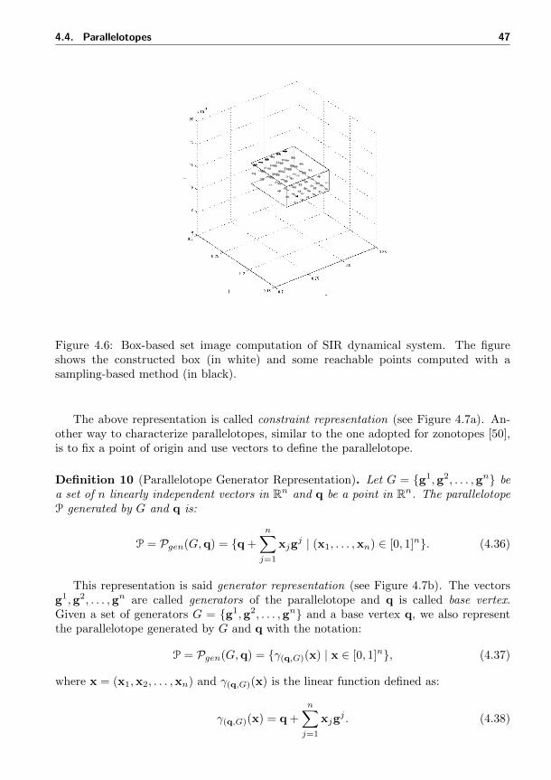
4.4. Parallelotopes 47
Figure 4.6: Box-based set image computation of SIR dynamical system. The figureshows the constructed box (in white) and some reachable points computed with asampling-based method (in black).
The above representation is called constraint representation (see Figure 4.7a). An-other way to characterize parallelotopes, similar to the one adopted for zonotopes [50],is to fix a point of origin and use vectors to define the parallelotope.
Definition 10 (Parallelotope Generator Representation). Let G = g1,g2, . . . ,gn bea set of n linearly independent vectors in Rn and q be a point in Rn. The parallelotopeP generated by G and q is:
P = Pgen(G,q) = q +
n∑j=1
xjgj | (x1, . . . ,xn) ∈ [0, 1]n. (4.36)
This representation is said generator representation (see Figure 4.7b). The vectorsg1,g2, . . . ,gn are called generators of the parallelotope and q is called base vertex.Given a set of generators G = g1,g2, . . . ,gn and a base vertex q, we also representthe parallelotope generated by G and q with the notation:
P = Pgen(G,q) = γ(q,G)(x) | x ∈ [0, 1]n, (4.37)
where x = (x1,x2, . . . ,xn) and γ(q,G)(x) is the linear function defined as:
γ(q,G)(x) = q +
n∑j=1
xjgj . (4.38)
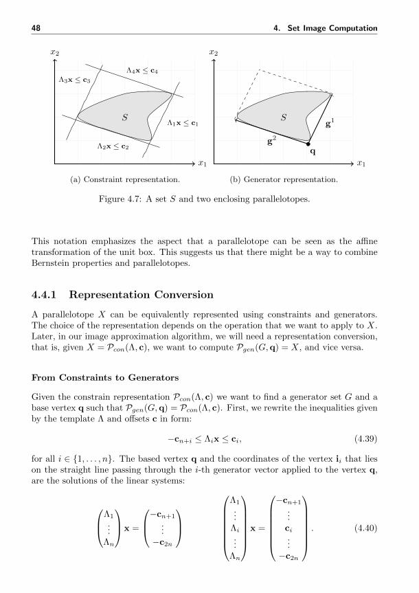
48 4. Set Image Computation
x2
x1
SΛ1x ≤ c1
Λ2x ≤ c2
Λ3x ≤ c3
Λ4x ≤ c4
(a) Constraint representation.
x2
x1
S
q
g1
g2
(b) Generator representation.
Figure 4.7: A set S and two enclosing parallelotopes.
This notation emphasizes the aspect that a parallelotope can be seen as the affinetransformation of the unit box. This suggests us that there might be a way to combineBernstein properties and parallelotopes.
4.4.1 Representation Conversion
A parallelotope X can be equivalently represented using constraints and generators.The choice of the representation depends on the operation that we want to apply to X.Later, in our image approximation algorithm, we will need a representation conversion,that is, given X = Pcon(Λ, c), we want to compute Pgen(G,q) = X, and vice versa.
From Constraints to Generators
Given the constrain representation Pcon(Λ, c) we want to find a generator set G and abase vertex q such that Pgen(G,q) = Pcon(Λ, c). First, we rewrite the inequalities givenby the template Λ and offsets c in form:
−cn+i ≤ Λix ≤ ci, (4.39)
for all i ∈ 1, . . . , n. The based vertex q and the coordinates of the vertex ii that lieson the straight line passing through the i-th generator vector applied to the vertex q,are the solutions of the linear systems:
Λ1
...Λn
x =
−cn+1
...−c2n
Λ1
...Λi...
Λn
x =
−cn+1
...ci...−c2n
. (4.40)
4.4. Parallelotopes 49
Hence, the i-th generator gi is the difference between the vertex vi and the base vertexq, i.e., gi = vi−q. Finally, the versor ui and the generator norm βi such that gi = βiui
are given by βi = ‖gi‖ and ui =gi
‖gi‖.
From Generators to Constraints
We now consider the inverse conversion: given a generator representation Pgen(G,q)we want to find a template Λ and a vector c such that Pcon(Λ, c) = Pgen(G,q). LetG = g1, . . . ,gn be the generator set and q be the base vertex.
As first step we calculate the points p1, . . . ,pn that are traversed by the hyper-planes correspondent to the constrains. Each pi is obtained by adding the generatorgi to the base vertex q, i.e., pi = q + gi. The i-th constraint of the parallelotopelies on the hyperplane (whose equation is πi = aix + ci) passing through the pointsq,p1, . . . ,pi−1,pi+1, . . . ,pn. The equation πi+n = ai+nx + ci+n of the hyperplane par-allel to πi can be found by translating the vertices used to compute πi by the vector gi,i.e., πi+n is the hyperplane passing through the points q+gi,p1+gi, . . . ,pi−1+gi,pi+1+gi, . . . ,pn + gi. Let ci and ci be defined as ci = mindi, di+n and ci = maxdi, di+n.
Since πi and πi+n are parallel it must hold ai = ai+n. Hence, the portion of theparallelotope included between πi and πi+n is the solution of the inequalities ci ≤ aix ≤ci, which means that the i-th and (i+n)-th rows of the template matrix are Λi = ai andΛi+n = −ai, while the i-th and (i+ n)-th offset elements are ci = ci and ci+n = −ci.
4.4.2 Parallelotope-Based Set Image
We now focus on the set image computation problem. Let X ⊂ Rn be a parallelo-tope whose constraint representation is X = Pcon(Λ, c) and generator representationis X = Pgen(G,q) (recall that γ(q,G)(x) is the linear function that defines the genera-tor representation, see Equation 4.38). We are interested in computing a parallelotopeX ′ ⊂ Rn such that f(X,P ) ⊆ X ′. Adopting the template Λ of X, we can obtain X ′ bydetermining the offsets c′ ∈ R2n such that f(X,P ) ⊆ Pcon(Λ, c′) = X ′.
In order for a parallelotope X ′ = 〈Λ, c′〉 in constraint representation to be an over-approximation of the set f(X,P ) it must hold that:
c′j ≥ maxx∈X,p∈P
Λjf(x,p) for all j ∈ 1, . . . , 2n. (4.41)
Then the inclusion f(X,P ) ⊆ Pcon(Λ, c) is guaranteed.
This condition can be rewritten using the generator representation as:
c′j ≥ maxx∈[0,1]n,p∈P
hj(x,p) for all j ∈ 1, . . . , 2n, (4.42)
where hj(x,p) = Λjf(γ(q,G)(x),p). Note that hj(x,p) is a polynomial function of xwhose domain is the unit box. Therefore, we can use Bernstein coefficients to computean upper bound c′j ∈ R of the function hj(x,p).
Let Bhj (p) = bi(p) | i ∈ Ihj be the set of Bernstein coefficients of the functionhj(x,p).
50 4. Set Image Computation
Theorem 1. Let c′ = (c′1, . . . , c′2n) be such that for each j ∈ 1, . . . , 2n the component
c′j is defined as:
c′j = maxbi(p) | i ∈ Ihj ,p ∈ P. (4.43)
The vector c′ satisfies the inclusion f(X,P ) ⊆ Pcon(Λ, c′).
Proof. It follows directly from Lemma 4 (range enclosing property of parametric Bern-stein coefficients) and Equation 4.42.
Before defining the algorithm for bounding the reachable set, we rewrite the generatorrepresentation explicitly distinguishing between the directions of the generators and theirlengths.
Let G = g1, . . . ,gn be a set of generators. Let βi ∈ R be the Euclidean normof gi and ui be the versor of gi, i.e., gi = βiu
i. Let β = (β1, . . . ,βn) and U =u1, . . . ,un. With a slight abuse of notation, we rewrite the generator representationof a parallelotope X as:
X = Pgen(q,β, U) = γU (q,β,x) | x ∈ [0, 1]n (4.44)
where γU (q,β,x) is the linear function of x defined as:
γU (q,β,x) = q +
n∑j=1
xjβjuj . (4.45)
When working on parallelotopes using the constraint representation, we can fix atemplate Λ and let the offset c free. In this way we symbolically denote an infinite setof parallelotopes. On the generator representation, this corresponds to fixing a set U ofn versors and letting the base vertex q and vector lengths β free.
Let us now focus on a single reachability step: given a parallelotopeX = Pcon(Λ, c) ⊂Rn and a polytopic parameter set P ⊂ Rm, we want to compute c′ ∈ R2n such thatPcon(Λ, c′) ⊂ Rn over-approximates the set f(X,P ). The set f(X,P ) can be character-ized as:
f(X,P ) = f(γU (q,β, [0, 1]n), P ) = f(γU (q,β,x),p) | x ∈ [0, 1]n,p ∈ P, (4.46)
where γU (q,β,x) is the generator function of X. Finding the base vertex q′ and thevector lengths β′ such that f(γU (q,β, [0, 1]n), P )) ⊆ γU (q′,β′, [0, 1]n) means obtainingan over-approximation in generator representation of f(X,P ). These q′ and β′ can befound thanks to the constraint representation.
Let Λ be the template matrix associated with the generator versors U . The offsetc′ such that f(γU (q,β, [0, 1]n), P ) ⊆ Pcon(Λ, c′) can be calculated using Theorem 1.That is, an upper bound of Λjf(γU (q,β, [0, 1]n), P ) can be found using the algorithmmaxBernCoeff (see Algorithm 1) based on Bernstein coefficients.
Let us algorithmically formalize these ideas. First, we define the algorithm bound(Algorithm 4) that receives in input a parametric polynomial π : Rn × Rm → R, aparallelotope X = 〈Λ, c〉 in constraint representation, and a polytopic parameter setP ⊂ Rm, and returns an upper bound b ∈ R of π(X,P ).
4.4. Parallelotopes 51
Algorithm 4 Bound polynomial over parallelotope and polytopic parameter set
1: function bound(π,X, P ) . X = 〈Λ, c〉 ⊂ Rn parallelotope, P ⊂ Rm polytope2: γU (q,β,x)←con2gen(X) . Compute generator function3: b←maxBernCoeff(π(γU (q,β,x), P ) . Compute maximum coefficient4: return b5: end function
The algorithm bound, using the function con2gen, converts the parallelotope Xfrom the constraint to the generator representation (Line 2), obtaining the generatorfunction γU (q,β,x). Then, it composes the polynomial π(x,p) with the generatorfunction γU (q,β,x) and, using the function maxBernCoeff, it determines an upperbound b of π(X,P ).
Thanks to the algorithm bound, we can now develop the parallelotope-based setimage algorithm reachStep (Algorithm 5) that, given a parametric polynomial func-tion f : Rn ×Rm → Rn, receives in input a parallelotope X = 〈Λ, c〉 ⊂ Rn in constraintrepresentation and a polytope P ⊂ Rm, and returns a parallelotope X = 〈Λ, c′〉 ⊂ Rnthat over-approximates the set f(X,P ).
Algorithm 5 Parallelotope-based reachability step
1: function reachStep(X,P ) . X = 〈Λ, c〉 ⊆ Rn parallelotope, P ⊆ Rm polytope2: for i ∈ 1, . . . , 2n do3: c′i ←bound(Λif(x,p), X, P )4: end for5: return X ′ = 〈Λ, c′〉6: end function
For each constraint of the parallelotope, the bounding functions Λif(x,p) are com-puted by composing the template directions Λi with the polynomial f(x,p). The upperbounds c′i are determined with the function bound, where Bernstein coefficients arecomputed and the values c′i are obtained by maximizing the parametric coefficients overthe parameter set P . The vector c′ is the offset that associated with the template Λconstitutes the searched approximation set X ′ = 〈Λ, c′〉 of f(X,P ).
Example 15. Consider the dynamics of the discrete-time SIR epidemic model of Ex-ample 6 with state variables and parameters grouped in the vectors x = (s, i, r) andp = (β, γ):
f(x,p) =
fs(x,p) = s− βsifi(x,p) = i+ βsi− γifr(x,p) = r + γi
(4.47)
52 4. Set Image Computation
Let X = Pcon(Λ, c) be the parallelotope in constraint representation defined as:
X = Λx ≤ c =
−1 0 0−1 −1 00 0 −11 0 01 1 00 0 1
x ≤
−0.80−0.950.000.851.000.00
(4.48)
and P = [0.35, 0.36] × [0.05, 0.06] be the parameter set with β ∈ [0.35, 0.36] and γ ∈[0.05, 0.06].
The equivalent generator representation of X is X = Pgen(q,β, U), with q =(0.80, 0.15, 0), β = (0.0707, 0.0500, 0.0000), and U = (0.7071,−0.7071, 0), (0, 1, 0),(0, 0, 1), whose generator function is:
γU (q,β,x) =
q1 + 0.7070β1sq2 − 0.7070β1s+ β2iq3 + rβ3
(4.49)
We now show how to bound the direction Λ1 = (−1, 0, 0). The composition h(x,p) =Λ1f(γU (q,β,x),p) is:
h(x,p) = (−1, 0, 0)
fs(γU (q,β,x),p)fi(γU (q,β,x),p)fr(γU (q,β,x),p)
= −fs(γU (q,β,x),p)
= −((q1 + 0.7070β1s)− β(q1 + 0.7070β1s)(q2 − 0.7070β1s+ β2i))
(4.50)
Instantiating the base vertex q and lengths β, we obtain the set of coefficients:
Bh = −0.8000 + 0.1200β,−0.8000 + 0.1600β,−0.8250 + 0.1038β,−0.8250 + 0.1450β,−0.8500 + 0.0850β,−0.8500 + 0.1275β,
(4.51)whose maximum over the parameter set P = [0.35, 0.36]×[0.05, 0.06], obtained by solvingsix linear programs, is c′1 = −0.7942.
Repeating the procedure for all the directions of the template Λ we obtain the vector ofoffsets c′ = (−0.7440,−0.9425,−0.0050, 0.8203, 0.9925, 0.0100) that, associated with thetemplate Λ, can be used to construct the over-approximating parallelotope X ′ = 〈Λ, c′〉 =Pcon(Λ, c′).
Figure 4.8 shows the constructed parallelotope X ′ (in white) with some reachablepoints (in black) computed with a sampling-based method. Note how X ′ contains all thecomputed points.
In this section we developed some methods to bound parametric polynomials overparallelotopes and compute parallelotopic over-approximations of set images. Parallelo-topes allow us to obtain approximations that are finer than the ones provided by boxes.However, in the next section, we will further improve in precision, exploiting sets ofparallelotopes and their intersections for the representation of sets of states reached bya dynamical system.
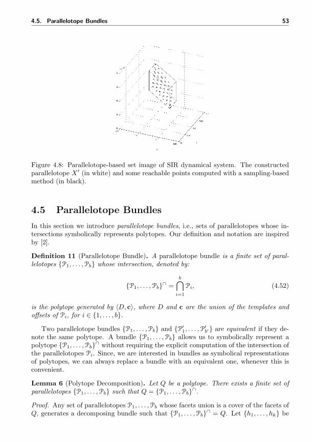
4.5. Parallelotope Bundles 53
Figure 4.8: Parallelotope-based set image of SIR dynamical system. The constructedparallelotope X ′ (in white) and some reachable points computed with a sampling-basedmethod (in black).
4.5 Parallelotope Bundles
In this section we introduce parallelotope bundles, i.e., sets of parallelotopes whose in-tersections symbolically represents polytopes. Our definition and notation are inspiredby [2].
Definition 11 (Parallelotope Bundle). A parallelotope bundle is a finite set of paral-lelotopes P1, . . . ,Pb whose intersection, denoted by:
P1, . . . ,Pb∩ =
b⋂i=1
Pi, (4.52)
is the polytope generated by 〈D, c〉, where D and c are the union of the templates andoffsets of Pi, for i ∈ 1, . . . , b.
Two parallelotope bundles P1, . . . ,Pb and P′1, . . . ,P′b′ are equivalent if they de-note the same polytope. A bundle P1, . . . ,Pb allows us to symbolically represent apolytope P1, . . . ,Pb∩ without requiring the explicit computation of the intersection ofthe parallelotopes Pi. Since, we are interested in bundles as symbolical representationsof polytopes, we can always replace a bundle with an equivalent one, whenever this isconvenient.
Lemma 6 (Polytope Decomposition). Let Q be a polytope. There exists a finite set ofparallelotopes P1, . . . ,Pb such that Q = P1, . . . ,Pb∩.
Proof. Any set of parallelotopes P1, . . . ,Pb whose facets union is a cover of the facets ofQ, generates a decomposing bundle such that P1, . . . ,Pb∩ = Q. Let h1, . . . , hk be
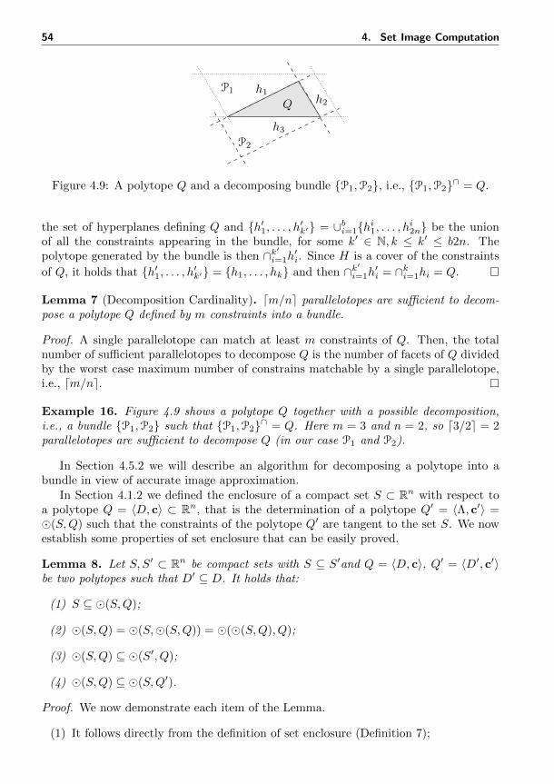
54 4. Set Image Computation
h1h2
h3
Q
P1
P2
Figure 4.9: A polytope Q and a decomposing bundle P1,P2, i.e., P1,P2∩ = Q.
the set of hyperplanes defining Q and h′1, . . . , h′k′ = ∪bi=1hi1, . . . , hi2n be the unionof all the constraints appearing in the bundle, for some k′ ∈ N, k ≤ k′ ≤ b2n. Thepolytope generated by the bundle is then ∩k
′
i=1h′i. Since H is a cover of the constraints
of Q, it holds that h′1, . . . , h′k′ = h1, . . . , hk and then ∩k′
i=1h′i = ∩ki=1hi = Q.
Lemma 7 (Decomposition Cardinality). dm/ne parallelotopes are sufficient to decom-pose a polytope Q defined by m constraints into a bundle.
Proof. A single parallelotope can match at least m constraints of Q. Then, the totalnumber of sufficient parallelotopes to decompose Q is the number of facets of Q dividedby the worst case maximum number of constrains matchable by a single parallelotope,i.e., dm/ne.
Example 16. Figure 4.9 shows a polytope Q together with a possible decomposition,i.e., a bundle P1,P2 such that P1,P2∩ = Q. Here m = 3 and n = 2, so d3/2e = 2parallelotopes are sufficient to decompose Q (in our case P1 and P2).
In Section 4.5.2 we will describe an algorithm for decomposing a polytope into abundle in view of accurate image approximation.
In Section 4.1.2 we defined the enclosure of a compact set S ⊂ Rn with respect toa polytope Q = 〈D, c〉 ⊂ Rn, that is the determination of a polytope Q′ = 〈Λ, c′〉 =(S,Q) such that the constraints of the polytope Q′ are tangent to the set S. We nowestablish some properties of set enclosure that can be easily proved.
Lemma 8. Let S, S′ ⊂ Rn be compact sets with S ⊆ S′and Q = 〈D, c〉, Q′ = 〈D′, c′〉be two polytopes such that D′ ⊆ D. It holds that:
(1) S ⊆ (S,Q);
(2) (S,Q) = (S,(S,Q)) = ((S,Q), Q);
(3) (S,Q) ⊆ (S′, Q);
(4) (S,Q) ⊆ (S,Q′).
Proof. We now demonstrate each item of the Lemma.
(1) It follows directly from the definition of set enclosure (Definition 7);
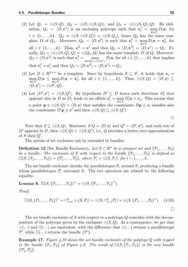
4.5. Parallelotope Bundles 55
(2) Let Q1 = (S,Q), Q2 = (S,(S,Q)), and Q3 = ((S,Q), Q). By defi-nition, Q1 = 〈D, c1〉 is an enclosing polytope such that c1i = max
x∈SDix, for
i ∈ 1, . . . , k. Q2 = (S,(S,Q)) = (S,Q1), hence Q2 has the same tem-plate D of Q1. Moreover, Q2 = 〈D, c2〉 is such that c2i = max
x∈SDix = c11, for
all i ∈ 1, . . . , k. Thus, c2 = c1 and then Q2 = 〈D, c2〉 = 〈D, c1〉 = Q1. Fi-nally, Q3 = ((S,Q), Q) = (Q1, Q) has the same template D of Q. Moreover,Q3 = 〈D, c3〉 is such that c3i = max
x∈Q1=〈D,c1〉Dix, for all i ∈ 1, . . . , k that implies
that c3i = c1i and then Q3 = 〈D, c3〉 = 〈D, c1〉 = Q1.
(3) Let D ∈ Rk×n be a template. Since by hypothesis S ⊆ S′, it holds that ci =maxx∈S
Dix ≤ maxx∈S′
Dix = c′i, for all i ∈ 1, . . . , k. Thus, (S,Q) = 〈D, c〉 ⊆〈D, c′〉 = (S′, Q).
(4) Let 〈D′, c′〉 = (S,Q′). By hypothesis D′ ⊆ D hence each directions D′i thatappears also in D as Dj leads to an offsets c′i = max
x∈SD′ix = cj . This means that
a point p ∈ (S,Q) = 〈D, c〉 that satisfies the constraints Dp ≤ c, satisfies alsothe constraints D′p ≤ c′ and then (S,Q) ⊆ (S,Q′).
Note that S ⊆ (S,Q). Moreover, if Q = 〈D, c〉 and Q′ = 〈D′, c′〉, and each row ofD′ appears in D, then (S,Q) ⊂ (S,Q′), i.e., Q provides a better over-approximationof S then Q′.
The notion of set enclosure can be extended to bundles.
Definition 12 (Set Bundle Enclosure). Let S ⊂ Rn be a compact set and P1, . . . ,Pbbe a bundle. The enclosure of S with respect to the bundle P1, . . . ,Pb is defined as(S, P1, . . . ,Pb) = P′1, . . . ,P′b, where P′i = (S,Pi), for i = 1, . . . , b.
The set bundle enclosure shrinks the parallelotopes Pi around S, producing a bundlewhose parallelotopes P′i surround S. The two operators are related by the followingequality.
Lemma 9. (S, P1, . . . ,Pb)∩ = (S, P1, . . . ,Pb∩).
Proof.
(S, P1, . . . , Pb)∩ = ∩bi=1 (S, Pi) = (S,∩bi=1Pi) = (S, P1, . . . , Pb∩) (4.53)
The set bundle enclosure of S with respect to a polytope Q coincides with the decom-position of the polytope given by the enclosure (S,Q). As a consequence, we get that(·, ·) and (·, ·) are equivalent, with the difference that (·, ·) returns a parallelotopeP′, while (·, ·) returns the bundle P′.
Example 17. Figure 4.10 shows the set bundle enclosure of the polytope Q with respectto the bundle P1,P2 of Figure 4.9. The result of (S, P1,P2) is the new bundleP′1,P′2.
56 4. Set Image Computation
h1h2
h3
QP′1
P′2
Figure 4.10: A polytope Q and a its set bundle enclosure with respect to P1,P2 ofFigure 4.9: (Q, P1,P2) = P′1,P′2.
We say that P′1, . . . ,P′b′ is a sub-bundle of the bundle P1, . . . ,Pb if P′1, . . . ,P′b′ ⊆P1, . . . ,Pb and that two bundles are strongly similar if the set of normal vectors defin-ing a parallelotope in one bundle is equal to the set of normal vectors defining a paral-lelotope in the other bundle. The following properties of the bundle enclosure operatorimmediately follow by definitions, Lemma 8, and Lemma 9.
Lemma 10. Let S, S′ ⊂ Rn be compact sets with S ⊆ S′, P1, . . . ,Pb be a bundle,P′1, . . . ,P′b′ be one of its sub-bundles, and P′′1 , . . . ,P′′b be a bundle strongly similar toP1, . . . ,Pb. It holds that:
(1) S ⊆ (S, P1, . . . ,Pb)∩;
(2) (S, P1, . . . ,Pb) = (S,(S, P1, . . . ,Pb)) = ((S, P1, . . . ,Pb), P1, . . . ,Pb);
(3) (S, P1, . . . ,Pb)∩ ⊆ (S′, P1, . . . ,Pb)∩;
(4) (S, P′1, . . . ,P′b′) ⊆ (S, P1, . . . ,Pb) and(S, P1, . . . ,Pb)∩ ⊆ (S, P′1, . . . ,P′b′)∩;
(5) (S, P1, . . . ,Pb) is strongly similar to P1, . . . ,Pb;
(6) (S, P1, . . . ,Pb) = (S, P′′1 , . . . ,P′′b ).
Proof. We now demonstrate each item of the Lemma.
(1) By Lemma 8 item (1) it holds that S ⊆ (S, Pi) ⊆ ∩bi=1(S, Pi) = (S, P1, . . . , Pb)∩.
(2) By Lemma 8 item (2) we know that for each Pi, with i ∈ 1, . . . , b it holds that(S, P1) = (S,(S, P1)) = ((S, P1), P1), from which it follows the thesis.
(3) It follows directly from Lemma 8 item (3).
(4) Similar to the previous cases but following from the item (4) of Lemma 8.
(5) By definition of set enclosure each parallelotope (S, Pi) of (S, P1, . . . , Pb) hasthe same template of Pi, for i ∈ 1, . . . , b.
(6) By hypothesis Pi and P ′′i have the same templates, for i ∈ 1, . . . , b. Thus(S, Pi) = (S, P ′′i ) from which it follows the thesis.
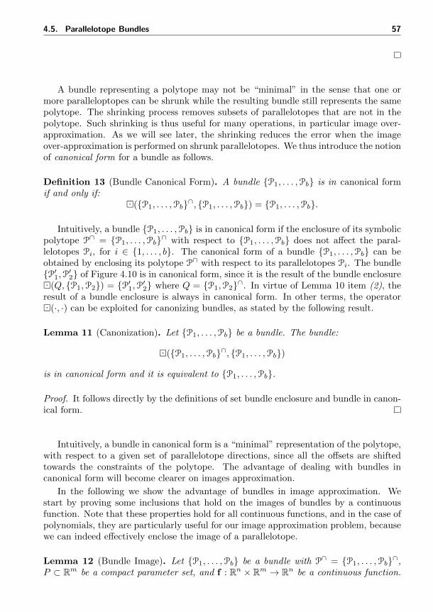
4.5. Parallelotope Bundles 57
A bundle representing a polytope may not be “minimal” in the sense that one ormore paralleloptopes can be shrunk while the resulting bundle still represents the samepolytope. The shrinking process removes subsets of parallelotopes that are not in thepolytope. Such shrinking is thus useful for many operations, in particular image over-approximation. As we will see later, the shrinking reduces the error when the imageover-approximation is performed on shrunk parallelotopes. We thus introduce the notionof canonical form for a bundle as follows.
Definition 13 (Bundle Canonical Form). A bundle P1, . . . ,Pb is in canonical formif and only if:
(P1, . . . ,Pb∩, P1, . . . ,Pb) = P1, . . . ,Pb.
Intuitively, a bundle P1, . . . ,Pb is in canonical form if the enclosure of its symbolicpolytope P∩ = P1, . . . ,Pb∩ with respect to P1, . . . ,Pb does not affect the paral-lelotopes Pi, for i ∈ 1, . . . , b. The canonical form of a bundle P1, . . . ,Pb can beobtained by enclosing its polytope P∩ with respect to its parallelotopes Pi. The bundleP′1,P′2 of Figure 4.10 is in canonical form, since it is the result of the bundle enclosure(Q, P1,P2) = P′1,P′2 where Q = P1,P2∩. In virtue of Lemma 10 item (2), theresult of a bundle enclosure is always in canonical form. In other terms, the operator(·, ·) can be exploited for canonizing bundles, as stated by the following result.
Lemma 11 (Canonization). Let P1, . . . ,Pb be a bundle. The bundle:
(P1, . . . ,Pb∩, P1, . . . ,Pb)
is in canonical form and it is equivalent to P1, . . . ,Pb.
Proof. It follows directly by the definitions of set bundle enclosure and bundle in canon-ical form.
Intuitively, a bundle in canonical form is a “minimal” representation of the polytope,with respect to a given set of parallelotope directions, since all the offsets are shiftedtowards the constraints of the polytope. The advantage of dealing with bundles incanonical form will become clearer on images approximation.
In the following we show the advantage of bundles in image approximation. Westart by proving some inclusions that hold on the images of bundles by a continuousfunction. Note that these properties hold for all continuous functions, and in the case ofpolynomials, they are particularly useful for our image approximation problem, becausewe can indeed effectively enclose the image of a parallelotope.
Lemma 12 (Bundle Image). Let P1, . . . ,Pb be a bundle with P∩ = P1, . . . ,Pb∩,P ⊂ Rm be a compact parameter set, and f : Rn × Rm → Rn be a continuous function.
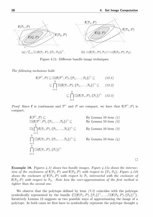
58 4. Set Image Computation
f(P1, P )
f(P2, P )f(Q,P )
(a) ∩2i=1 (f(Pi, P ), P1,P2)∩.
f(P1, P )
f(P2, P )f(Q,P )
(b) (f(P1, P ),P1) ∩ (f(P2, P ),P2).
Figure 4.11: Different bundle image techniques.
The following inclusions hold:
f(P∩, P ) ⊆ (f(P∩, P ), P1, . . . ,Pb)∩ ⊆ (12.1)
⊆b⋂i=1
(f(Pi, P ), P1, . . . ,Pb)∩ ⊆ (12.2)
⊆b⋂i=1
(f(Pi, P ), Pi)∩ (12.3)
Proof. Since f is continuous and P∩ and P are compact, we have that f(P∩, P ) iscompact.
f(P∩, P ) ⊆ By Lemma 10 item (1)(f(P∩, P ), P1, . . . ,Pb)∩ ⊆ By Lemma 10 item (3)
(
b⋂i=1
f(Pi, P ), P1, . . . ,Pb)∩ ⊆ By Lemma 10 item (3)
b⋂i=1
(f(Pi, P ), P1, . . . ,Pb)∩ ⊆ By Lemma 10 item (4)
b⋂i=1
(f(Pi, P ), Pi)∩
Example 18. Figures 4.11 shows two bundle images. Figure 4.11a shows the intersec-tion of the enclosures of f(P1, P ) and f(P2, P ) with respect to P1,P2; Figure 4.11bshows the enclosure of f(P1, P ) with respect to P1 intersected with the enclosure off(P2, P ) with respect to P2. Note how the over-approximation of the first method istighter than the second one.
We observe that the polytope defined by item (7.3) coincides with the polytopesymbolically represented by the bundle (f(P1, P ), P1)∩, . . . ,(f(Pb, P ), Pb)∩.Intuitively Lemma 12 suggests us two possible ways of approximating the image of apolytope. In both cases we first have to symbolically represent the polytope thought a
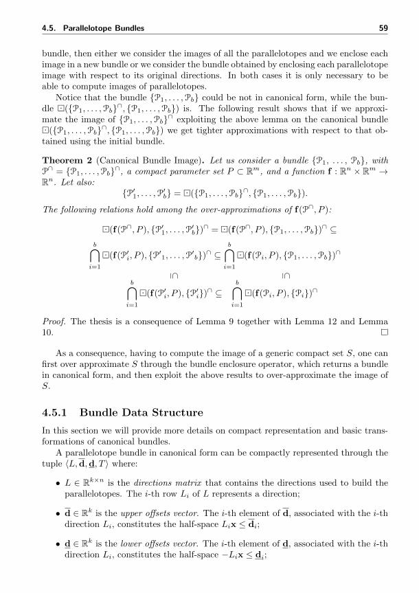
4.5. Parallelotope Bundles 59
bundle, then either we consider the images of all the parallelotopes and we enclose eachimage in a new bundle or we consider the bundle obtained by enclosing each parallelotopeimage with respect to its original directions. In both cases it is only necessary to beable to compute images of parallelotopes.
Notice that the bundle P1, . . . ,Pb could be not in canonical form, while the bun-dle (P1, . . . ,Pb∩, P1, . . . ,Pb) is. The following result shows that if we approxi-mate the image of P1, . . . ,Pb∩ exploiting the above lemma on the canonical bundle(P1, . . . ,Pb∩, P1, . . . ,Pb) we get tighter approximations with respect to that ob-tained using the initial bundle.
Theorem 2 (Canonical Bundle Image). Let us consider a bundle P1, . . . , Pb, withP∩ = P1, . . . ,Pb∩, a compact parameter set P ⊂ Rm, and a function f : Rn × Rm →Rn. Let also:
P′1, . . . ,P′b = (P1, . . . ,Pb∩, P1, . . . ,Pb).
The following relations hold among the over-approximations of f(P∩, P ):
(f(P∩, P ), P′1, . . . ,P′b)∩ = (f(P∩, P ), P1, . . . ,Pb)∩ ⊆b⋂i=1
(f(P′i, P ), P′1, . . . ,P′b)∩ ⊆b⋂i=1
(f(Pi, P ), P1, . . . ,Pb)∩⊆ ⊆
b⋂i=1
(f(P′i, P ), P′i)∩ ⊆b⋂i=1
(f(Pi, P ), Pi)∩
Proof. The thesis is a consequence of Lemma 9 together with Lemma 12 and Lemma10.
As a consequence, having to compute the image of a generic compact set S, one canfirst over approximate S through the bundle enclosure operator, which returns a bundlein canonical form, and then exploit the above results to over-approximate the image ofS.
4.5.1 Bundle Data Structure
In this section we will provide more details on compact representation and basic trans-formations of canonical bundles.
A parallelotope bundle in canonical form can be compactly represented through thetuple 〈L,d,d, T 〉 where:
• L ∈ Rk×n is the directions matrix that contains the directions used to build theparallelotopes. The i-th row Li of L represents a direction;
• d ∈ Rk is the upper offsets vector. The i-th element of d, associated with the i-thdirection Li, constitutes the half-space Lix ≤ di;
• d ∈ Rk is the lower offsets vector. The i-th element of d, associated with the i-thdirection Li, constitutes the half-space −Lix ≤ di;
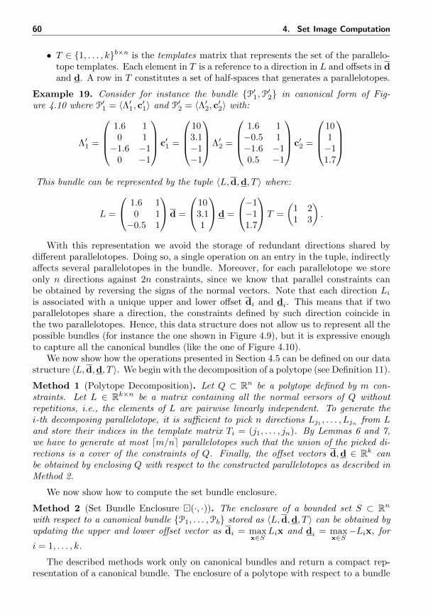
60 4. Set Image Computation
• T ∈ 1, . . . , kb×n is the templates matrix that represents the set of the parallelo-tope templates. Each element in T is a reference to a direction in L and offsets in dand d. A row in T constitutes a set of half-spaces that generates a parallelotopes.
Example 19. Consider for instance the bundle P′1,P′2 in canonical form of Fig-ure 4.10 where P′1 = 〈Λ′1, c′1〉 and P′2 = 〈Λ′2, c′2〉 with:
Λ′1 =
1.6 10 1−1.6 −1
0 −1
c′1 =
103.1−1−1
Λ′2 =
1.6 1−0.5 1−1.6 −10.5 −1
c′2 =
101−11.7
This bundle can be represented by the tuple 〈L,d,d, T 〉 where:
L =
1.6 10 1−0.5 1
d =
103.11
d =
−1−11.7
T =
(1 21 3
).
With this representation we avoid the storage of redundant directions shared bydifferent parallelotopes. Doing so, a single operation on an entry in the tuple, indirectlyaffects several parallelotopes in the bundle. Moreover, for each parallelotope we storeonly n directions against 2n constraints, since we know that parallel constraints canbe obtained by reversing the signs of the normal vectors. Note that each direction Liis associated with a unique upper and lower offset di and di. This means that if twoparallelotopes share a direction, the constraints defined by such direction coincide inthe two parallelotopes. Hence, this data structure does not allow us to represent all thepossible bundles (for instance the one shown in Figure 4.9), but it is expressive enoughto capture all the canonical bundles (like the one of Figure 4.10).
We now show how the operations presented in Section 4.5 can be defined on our datastructure 〈L,d,d, T 〉. We begin with the decomposition of a polytope (see Definition 11).
Method 1 (Polytope Decomposition). Let Q ⊂ Rn be a polytope defined by m con-straints. Let L ∈ Rk×n be a matrix containing all the normal versors of Q withoutrepetitions, i.e., the elements of L are pairwise linearly independent. To generate thei-th decomposing parallelotope, it is sufficient to pick n directions Lj1 , . . . , Ljn from Land store their indices in the template matrix Ti = (j1, . . . , jn). By Lemmas 6 and 7,we have to generate at most dm/ne parallelotopes such that the union of the picked di-rections is a cover of the constraints of Q. Finally, the offset vectors d,d ∈ Rk canbe obtained by enclosing Q with respect to the constructed parallelotopes as described inMethod 2.
We now show how to compute the set bundle enclosure.
Method 2 (Set Bundle Enclosure (·, ·)). The enclosure of a bounded set S ⊂ Rnwith respect to a canonical bundle P1, . . . ,Pb stored as 〈L,d,d, T 〉 can be obtained byupdating the upper and lower offset vector as di = max
x∈SLix and di = max
x∈S−Lix, for
i = 1, . . . , k.
The described methods work only on canonical bundles and return a compact rep-resentation of a canonical bundle. The enclosure of a polytope with respect to a bundle
4.5. Parallelotope Bundles 61
requires the resolution of 2k linear programs. Thus, the canonization of a bundle canbe done by solving a series of linear programs where only the offsets of the constraintsthat do not participate to the intersection are modified.
The transformation of a bundle through a continuous function can be rather diffi-cult, depending on the transforming function. If the function is linear, it is possible toexactly compute the image of each parallelotope and then obtain the exact bundle trans-formation. Things are more complex when the function is nonlinear and the geometricproperties of the parallelotopes are not preserved. We will now describe two methods,based on Theorem 2, that only require to be able to compute the image of a parallelo-tope, besides being able to implement Method 2. As stated by Lemma 12 item (3), anover-approximation of a bundle transformation f(P∩, P ), with P∩ = P1, . . . ,Pb, canbe obtained by enclosing each image f(Pi, P ) with P′i = (f(Pi, P ), Pi)∩ and thenconsidering the intersection ∩bi=1P
′i (see (12.3)). We call such approximation one-for-one
(OFO), since each parallelotope in the bundle is independently approximated.
Method 3 (One-for-One Image (OFO)). The one-for-one approximation of the bundle〈L,d,d, T 〉 can be obtained by retrieving each parallelotope Pi, computing the enclosuresP′i = (f(Pi, P ),Pi), and then computing the canonization of P′1, . . . ,P′b∩ = P′∩, thatis (P′∩, P′1, . . . ,P′b).
The polytope provided by the OFO method corresponds to the set ∩bi=1(f(Pi, P ), Pi)∩of Theorem 2.
In order to obtain a finer over-approximation, it is possible to change the templatein the approximation process, i.e., we can fix a new template to enclose f(Pi, P ). Assuggested by Lemma 12 item (2), we can exploit all the directions of the bundle, i.e.,instead of looking for a new template for each parallelotope, we can bound each setf(Pi, P ) with all the directions of the starting bundle. We call such approximation all-for-one (AFO) since all the directions of the bundle are used to approximate the imageof a single parallelotope.
Method 4 (All-for-One Image (AFO)). The all-for-one approximation of the bundle〈L,d,d, T 〉 can be obtained by retrieving each parallelotope Pi, computing the set bundleenclosure P′i1, . . . ,P
′ib = (f(Pi, P ), P1, . . . ,Pb), and then decomposing the polytope
∩bi=1P′i1, . . . ,P′ib∩, i.e., computing (∩bi=1P′i1, . . . ,P
′ib∩, P1, . . . ,Pb).
The AFO transformation produces a bundle whose symbolic polytope correspondsto the polytope of the left-hand side term of the last line in Theorem 2. By Theorem 2,the AFO approximation is finer than the one produced by the OFO method. Obviouslythe precision has a cost: the OFO method requires b(2n) + k optimizations against theb(2k) + k optimizations of the AFO approach (recall that k ≥ n).
Both the approximation methods are based on a series of enclosures. The offsetsof the constraints necessary to obtain the enclosures, can be attained by solving opti-mization problems of the form dj = max
x∈f(Pi,P )Ljx. If the transformation function f is
nonlinear, these optimization problems might be computationally expensive. However,in the next section we expose a method, based on the Bernstein coefficients, to efficientlydeal with images of polynomial functions.
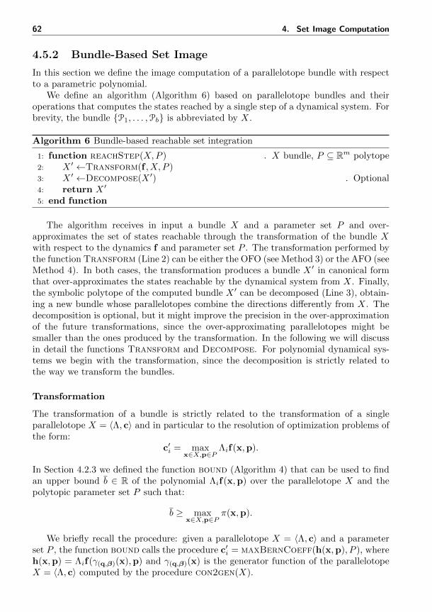
62 4. Set Image Computation
4.5.2 Bundle-Based Set Image
In this section we define the image computation of a parallelotope bundle with respectto a parametric polynomial.
We define an algorithm (Algorithm 6) based on parallelotope bundles and theiroperations that computes the states reached by a single step of a dynamical system. Forbrevity, the bundle P1, . . . ,Pb is abbreviated by X.
Algorithm 6 Bundle-based reachable set integration
1: function reachStep(X,P ) . X bundle, P ⊆ Rm polytope2: X ′ ←Transform(f , X, P )3: X ′ ←Decompose(X ′) . Optional4: return X ′
5: end function
The algorithm receives in input a bundle X and a parameter set P and over-approximates the set of states reachable through the transformation of the bundle Xwith respect to the dynamics f and parameter set P . The transformation performed bythe function Transform (Line 2) can be either the OFO (see Method 3) or the AFO (seeMethod 4). In both cases, the transformation produces a bundle X ′ in canonical formthat over-approximates the states reachable by the dynamical system from X. Finally,the symbolic polytope of the computed bundle X ′ can be decomposed (Line 3), obtain-ing a new bundle whose parallelotopes combine the directions differently from X. Thedecomposition is optional, but it might improve the precision in the over-approximationof the future transformations, since the over-approximating parallelotopes might besmaller than the ones produced by the transformation. In the following we will discussin detail the functions Transform and Decompose. For polynomial dynamical sys-tems we begin with the transformation, since the decomposition is strictly related tothe way we transform the bundles.
Transformation
The transformation of a bundle is strictly related to the transformation of a singleparallelotope X = 〈Λ, c〉 and in particular to the resolution of optimization problems ofthe form:
c′i = maxx∈X,p∈P
Λif(x,p).
In Section 4.2.3 we defined the function bound (Algorithm 4) that can be used to findan upper bound b ∈ R of the polynomial Λif(x,p) over the parallelotope X and thepolytopic parameter set P such that:
b ≥ maxx∈X,p∈P
π(x,p).
We briefly recall the procedure: given a parallelotope X = 〈Λ, c〉 and a parameterset P , the function bound calls the procedure c′i = maxBernCoeff(h(x,p), P ), whereh(x,p) = Λif(γ(q,β)(x),p) and γ(q,β)(x) is the generator function of the parallelotopeX = 〈Λ, c〉 computed by the procedure con2gen(X).
4.5. Parallelotope Bundles 63
We now see how the function Bound can be used to define our bundle transformationmethods.
The OFO transformation of a bundle 〈L,d,d, T 〉 with parameter set P ⊂ Rn, asexposed in Method 3, can be obtained by retrieving each parallelotope Pi = 〈Λ, c〉, fori = 1, . . . , b, computing the new offsets c′j = Bound(Λjf(x,p),Pi, P ), for j = 1, . . . , 2n,and defining the over-approximating parallelotope P′i = 〈Λ, c′〉 ⊇ f(Pi, P ). Finally,the canonization of the transformed bundle P′1, . . . ,P′b can be obtained by solvinga family of linear programs of the form max
x∈P′∩Λix, where Λi belongs to the template
matrices of P′j and P′∩ = P′1, . . . ,P′b∩ is the polytope of the computed bundle.
The AFO transformation of a bundle 〈L,d,d, T 〉 with parameter set P , as definedin Method 4, can be done as follows. For each parallelotope of the bundle Pi, for i =1, . . . , b, we have to compute the enclosure P′i1, . . . ,P
′ib = (f(Pi, P ), P1, . . . ,Pb).
An over-approximation of P′im is the parallelotope 〈Λ, c′〉 where Λ is the template ofPim and c′j = Bound(Λjf(x,p),Pim , P ), for all j = 1, . . . , 2n. Finally, the canonization
enclosure (∩bi=1P′i1, . . . ,P′ib∩, P1, . . . ,Pb) can be computed by solving a group of
linear programs of the form maxx∈P′∩
Λjx, where Λj belongs to the template matrices of
P′im and P′∩ = ∩bi=1P′i1, . . . ,P′ib∩ is the polytope obtained by the intersection of the
polytopes of the computed bundles.
Decomposition
Since in our reachability algorithm (see Algorithm 6) we are interested in decomposing apolytope described by a bundle, we define a function Decompose that receives in inputa bundle in canonical form 〈L,d,d, T 〉 (whose polytope P∩ has to be decomposed) andreorganizes the templates matrix T creating a new collection of parallelotopes aroundthe polytope P∩. The goal of the decomposition is to create a set of small parallelotopeswhose intersection is P∩. There are two reasons why we want small parallelotopes:
1. Smaller parallelotopes Pi lead to a smaller bundle image f(P1, P ), . . . , f(Pd, P )and then to a more accurate over-approximation f(P∩, P ) (see, e.g., Theorem 2);
2. The shorter the largest side length of Pi, the more accurate the over-approximationintroduced by the Bernstein coefficients (see Lemma 3).
The aspects to take into account in the construction of the parallelotopes are: thevolume and the maximum side length. Moreover, we do not have to forget that the setof the parallelotope directions must cover the directions of the decomposed symbolicpolytope (see Definition 11). Finding the best decomposition in terms of volume andmaximum length minimization is computationally expensive and might not be possible(recall that the set cover problem is NP-hard).
In order to efficiently find a good decomposition, we propose a heuristic techniquethat constructs the parallelotopes while trying to minimize the volumes and maximumside lengths. The proposed heuristic starts from a decomposition, applies a series ofrandom changes to the templates matrix, and keeps only the best one accordingly toan evaluation function that we will soon define. The procedure is repeated until a fixednumber of iterations is reached.
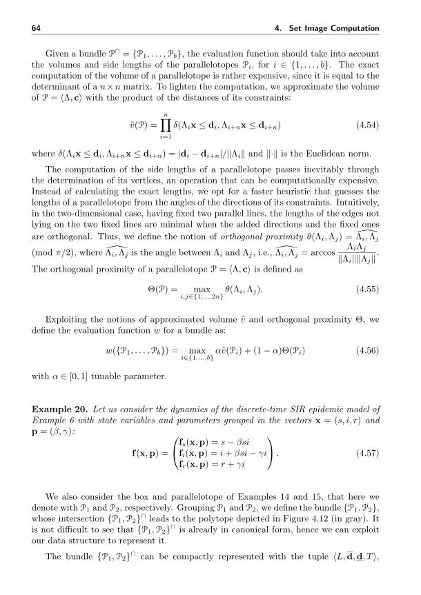
64 4. Set Image Computation
Given a bundle P∩ = P1, . . . ,Pb, the evaluation function should take into accountthe volumes and side lengths of the parallelotopes Pi, for i ∈ 1, . . . , b. The exactcomputation of the volume of a parallelotope is rather expensive, since it is equal to thedeterminant of a n×n matrix. To lighten the computation, we approximate the volumeof P = 〈Λ, c〉 with the product of the distances of its constraints:
v(P) =n∏i=1
δ(Λix ≤ di,Λi+nx ≤ di+n) (4.54)
where δ(Λix ≤ di,Λi+nx ≤ di+n) = |di − di+n|/‖Λi‖ and ‖·‖ is the Euclidean norm.
The computation of the side lengths of a parallelotope passes inevitably throughthe determination of its vertices, an operation that can be computationally expensive.Instead of calculating the exact lengths, we opt for a faster heuristic that guesses thelengths of a parallelotope from the angles of the directions of its constraints. Intuitively,in the two-dimensional case, having fixed two parallel lines, the lengths of the edges notlying on the two fixed lines are minimal when the added directions and the fixed ones
are orthogonal. Thus, we define the notion of orthogonal proximity θ(Λi,Λj) = Λi,Λj
(mod π/2), where Λi,Λj is the angle between Λi and Λj , i.e., Λi,Λj = arccosΛiΛj
‖Λi‖‖Λj‖.
The orthogonal proximity of a parallelotope P = 〈Λ, c〉 is defined as
Θ(P) = maxi,j∈1,...,2n
θ(Λi,Λj). (4.55)
Exploiting the notions of approximated volume v and orthogonal proximity Θ, wedefine the evaluation function w for a bundle as:
w(P1, . . . ,Pb) = maxi∈1,...,b
αv(Pi) + (1− α)Θ(Pi) (4.56)
with α ∈ [0, 1] tunable parameter.
Example 20. Let us consider the dynamics of the discrete-time SIR epidemic model ofExample 6 with state variables and parameters grouped in the vectors x = (s, i, r) andp = (β, γ):
f(x,p) =
fs(x,p) = s− βsifi(x,p) = i+ βsi− γifr(x,p) = r + γi
. (4.57)
We also consider the box and parallelotope of Examples 14 and 15, that here wedenote with P1 and P2, respectively. Grouping P1 and P2, we define the bundle P1,P2,whose intersection P1,P2∩ leads to the polytope depicted in Figure 4.12 (in gray). Itis not difficult to see that P1,P2∩ is already in canonical form, hence we can exploitour data structure to represent it.
The bundle P1,P2∩ can be compactly represented with the tuple 〈L,d,d, T 〉,
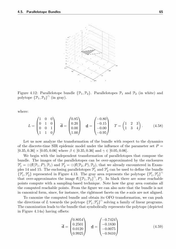
4.5. Parallelotope Bundles 65
Figure 4.12: Parallelotope bundle P1,P2. Parallelotopes P1 and P2 (in white) andpolytope P1,P2∩ (in gray).
where:
L =
1 0 00 1 00 0 11 1 0
d =
0.850.200.001.00
d =
−0.80−0.15−0.00−0.95
T =
(1 2 31 3 4
). (4.58)
Let us now analyze the transformation of the bundle with respect to the dynamicsof the discrete-time SIR epidemic model under the influence of the parameter set P =[0.35, 0.36]× [0.05, 0.06] where β ∈ [0.35, 0.36] and γ ∈ [0.05, 0.06].
We begin with the independent transformation of parallelotopes that compose thebundle. The images of the parallelotopes can be over-approximated by the enclosuresP′1 = (f(P1, P ),P1) and P′2 = (f(P2, P ),P2), that we already encountered in Exam-ples 14 and 15. The enclosing parallelotopes P′1 and P′2 can be used to define the bundleP′1,P′2 represented in Figure 4.13. The gray area represents the polytope P′1,P′2∩that over-approximates the image f(P1,P2∩, P ). In black there are some reachablepoints compute with a sampling-based technique. Note how the gray area contains allthe computed reachable points. From the figure we can also note that the bundle is notin canonical form, since, for instance, the rightmost facets on the s-axis are not aligned.
To canonize the computed bundle and obtain its OFO transformation, we can pushthe directions of L towards the polytope P′1,P′2∩ solving a family of linear programs.The canonization leads to the bundle that symbolically represents the polytope (depictedin Figure 4.14a) having offsets:
d =
0.80540.25010.01200.9925
d =
−0.7424−0.1830−0.0075−0.9410
(4.59)
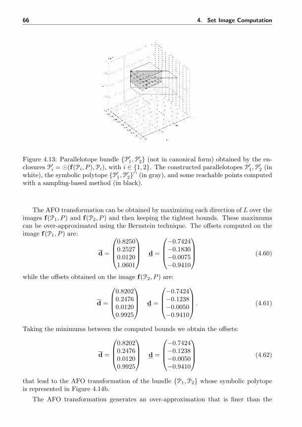
66 4. Set Image Computation
Figure 4.13: Parallelotope bundle P′1,P′2 (not in canonical form) obtained by the en-closures P′i = (f(Pi, P ),Pi), with i ∈ 1, 2. The constructed parallelotopes P′1,P
′2 (in
white), the symbolic polytope P′1,P′2∩ (in gray), and some reachable points computedwith a sampling-based method (in black).
The AFO transformation can be obtained by maximizing each direction of L over theimages f(P1, P ) and f(P2, P ) and then keeping the tightest bounds. These maximumscan be over-approximated using the Bernstein technique. The offsets computed on theimage f(P1, P ) are:
d =
0.82500.25270.01201.0601
d =
−0.7424−0.1830−0.0075−0.9410
(4.60)
while the offsets obtained on the image f(P2, P ) are:
d =
0.82020.24760.01200.9925
d =
−0.7424−0.1238−0.0050−0.9410
. (4.61)
Taking the minimums between the computed bounds we obtain the offsets:
d =
0.82020.24760.01200.9925
d =
−0.7424−0.1238−0.0050−0.9410
(4.62)
that lead to the AFO transformation of the bundle P1,P2 whose symbolic polytopeis represented in Figure 4.14b.
The AFO transformation generates an over-approximation that is finer than the
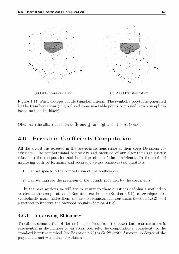
4.6. Bernstein Coefficients Computation 67
(a) OFO transformation. (b) AFO transformation.
Figure 4.14: Parallelotope bundle transformations. The symbolic polytopes generatedby the transformations (in gray) and some reachable points computed with a sampling-based method (in black).
OFO one (the offsets coefficients d1 and d1 are tighter in the AFO case).
4.6 Bernstein Coefficients Computation
All the algorithms exposed in the previous sections share at their cores Bernstein co-efficients. The computational complexity and precision of our algorithms are strictlyrelated to the computation and bound precision of the coefficients. In the spirit ofimproving both performance and accuracy, we ask ourselves two questions:
1. Can we speed-up the computation of the coefficients?
2. Can we improve the precision of the bounds provided by the coefficients?
In the next sections we will try to answer to these questions defining a method toaccelerate the computation of Bernstein coefficients (Section 4.6.1), a technique thatsymbolically manipulates them and avoids redundant computations (Section 4.6.2), anda method to improve the provided bounds (Section 4.6.3).
4.6.1 Improving Efficiency
The direct computation of Bernstein coefficients from the power base representation isexponential in the number of variables, precisely, the computational complexity of thestandard iterative method (see Equation 4.20) is O(d2n) with d maximum degree of thepolynomial and n number of variables.
68 4. Set Image Computation
The Matrix method [168] is a technique based on operations on matrices that avoidsredundant computations and reduces the computational complexity by a multiplica-tive factor to O(dn+1). In [176] an efficient symbolic method for restricting the set ofcoefficients that contains the upper bound is proposed. Unluckily, this technique cannot be applied to parametric polynomials since it requires the numerical knowledge ofthe coefficients of the treated polynomial in power base. However, we now propose animprovement of the matrix method that can reduce further the complexity of this tech-nique. The gain in efficiency relies in a fast transposition of multidimensional matrices.
The Matrix Method
The main idea of the Matrix method is to express Bernstein coefficients as a series ofmatrix products. For instance, the univariate polynomial2 π(x,p) : R× Rm → R, thatcan be expressed in both power and Bernstein basis as (see Section 4.2):
π(x,p) =
d∑i=1
ai(p)xi =
d∑i=1
bi(p)B(d,i)(x), (4.63)
can also be rewritten as:
π(x,p) = (1, x, x2, . . . , xd)
a0(p)...
ad(p)
= Xa(p), (4.64)
or as:
π(x,p) = (B(d,0)(x),B(d,1)(x), . . . ,B(d,d)(x))
b0(p)...
bd(p)
= Bb(p), (4.65)
where B(d,i)(x) is the i-th Bernstein polynomial of degree d and bi(p) is a parametricBernstein coefficient, with i ∈ Iπ.
Defining the matrix:
Ux =
1 0 0 . . . 0
1
(1
0
)(d
1
)−10 . . . 0
1
(2
1
)(d
1
)−1 (2
0
)(d
2
)−1. . . 0
......
.... . .
...1 1 1 1 1
(4.66)
for the unit box domain, it holds that π(x,p) = Bb(p) = XU−1x b(p) from whichfollows b(p) = Uxa(p) [168]. Thus, to obtain the vector of Bernstein coefficients b(p)
2We use the notation π(x,p) instead of π(x,p) to stress the fact that the vector x has only oneelement and the indices i and d are scalars.
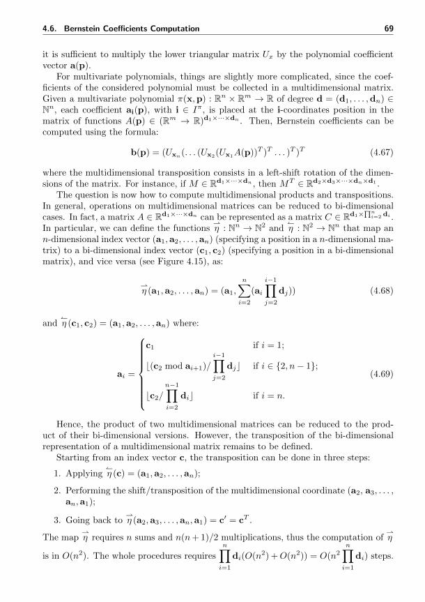
4.6. Bernstein Coefficients Computation 69
it is sufficient to multiply the lower triangular matrix Ux by the polynomial coefficientvector a(p).
For multivariate polynomials, things are slightly more complicated, since the coef-ficients of the considered polynomial must be collected in a multidimensional matrix.Given a multivariate polynomial π(x,p) : Rn × Rm → R of degree d = (d1, . . . ,dn) ∈Nn, each coefficient ai(p), with i ∈ Iπ, is placed at the i-coordinates position in thematrix of functions A(p) ∈ (Rm → R)d1×···×dn . Then, Bernstein coefficients can becomputed using the formula:
b(p) = (Uxn(. . . (Ux2(Ux1A(p))T )T . . . )T )T (4.67)
where the multidimensional transposition consists in a left-shift rotation of the dimen-sions of the matrix. For instance, if M ∈ Rd1×···×dn , then MT ∈ Rd2×d3×···×dn×d1 .
The question is now how to compute multidimensional products and transpositions.In general, operations on multidimensional matrices can be reduced to bi-dimensionalcases. In fact, a matrix A ∈ Rd1×···×dn can be represented as a matrix C ∈ Rd1×
∏ni=2 di .
In particular, we can define the functionsη : Nn → N2 and
η : N2 → Nn that map an
n-dimensional index vector (a1,a2, . . . ,an) (specifying a position in a n-dimensional ma-trix) to a bi-dimensional index vector (c1, c2) (specifying a position in a bi-dimensionalmatrix), and vice versa (see Figure 4.15), as:
η (a1,a2, . . . ,an) = (a1,
n∑i=2
(ai
i−1∏j=2
dj)) (4.68)
andη (c1, c2) = (a1,a2, . . . ,an) where:
ai =
c1 if i = 1;
b(c2 mod ai+1)/i−1∏j=2
djc if i ∈ 2, n− 1;
bc2/n−1∏i=2
dic if i = n.
(4.69)
Hence, the product of two multidimensional matrices can be reduced to the prod-uct of their bi-dimensional versions. However, the transposition of the bi-dimensionalrepresentation of a multidimensional matrix remains to be defined.
Starting from an index vector c, the transposition can be done in three steps:
1. Applyingη (c) = (a1,a2, . . . ,an);
2. Performing the shift/transposition of the multidimensional coordinate (a2, a3, . . . ,an,a1);
3. Going back toη (a2,a3, . . . ,an,a1) = c′ = cT .
The mapη requires n sums and n(n+ 1)/2 multiplications, thus the computation of
η
is in O(n2). The whole procedures requires
n∏i=1
di(O(n2) +O(n2)) = O(n2n∏i=1
di) steps.
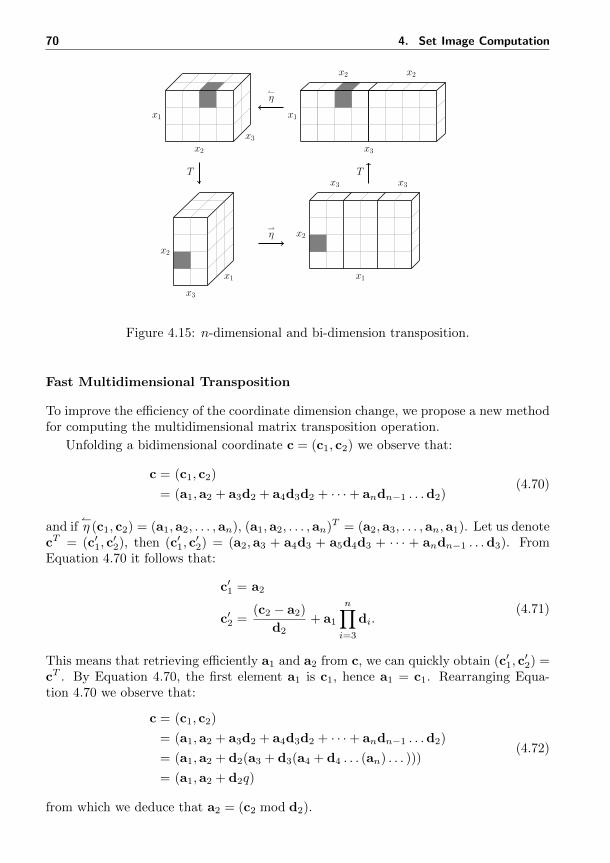
70 4. Set Image Computation
T T
η
η
x1
x2
x3
x1
x3
x2 x2
x2
x3
x1
x2
x1
x3 x3
Figure 4.15: n-dimensional and bi-dimension transposition.
Fast Multidimensional Transposition
To improve the efficiency of the coordinate dimension change, we propose a new methodfor computing the multidimensional matrix transposition operation.
Unfolding a bidimensional coordinate c = (c1, c2) we observe that:
c = (c1, c2)
= (a1,a2 + a3d2 + a4d3d2 + · · ·+ andn−1 . . .d2)(4.70)
and ifη (c1, c2) = (a1,a2, . . . ,an), (a1,a2, . . . ,an)T = (a2,a3, . . . ,an,a1). Let us denote
cT = (c′1, c′2), then (c′1, c
′2) = (a2,a3 + a4d3 + a5d4d3 + · · · + andn−1 . . .d3). From
Equation 4.70 it follows that:
c′1 = a2
c′2 =(c2 − a2)
d2+ a1
n∏i=3
di.(4.71)
This means that retrieving efficiently a1 and a2 from c, we can quickly obtain (c′1, c′2) =
cT . By Equation 4.70, the first element a1 is c1, hence a1 = c1. Rearranging Equa-tion 4.70 we observe that:
c = (c1, c2)
= (a1,a2 + a3d2 + a4d3d2 + · · ·+ andn−1 . . .d2)
= (a1,a2 + d2(a3 + d3(a4 + d4 . . . (an) . . . )))
= (a1,a2 + d2q)
(4.72)
from which we deduce that a2 = (c2 mod d2).
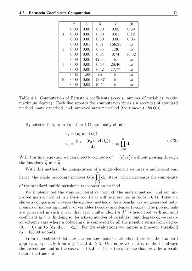
4.6. Bernstein Coefficients Computation 71
2 3 5 7 100.00 0.00 0.00 0.02 0.69
1 0.00 0.00 0.00 0.01 0.120.00 0.00 0.00 0.00 0.050.00 0.01 0.81 166.35 to
3 0.00 0.00 0.05 1.36 to0.00 0.00 0.04 0.74 76.520.00 0.06 42.84 to to
5 0.00 0.00 0.48 28.46 to0.00 0.00 0.32 17.77 to0.02 1.88 to to to
10 0.00 0.06 13.87 to to0.00 0.05 10.54 to to
Table 4.1: Computation of Bernstein coefficients (x-axis: number of variables, y-axis:maximum degree). Each line reports the computation times (in seconds) of standardmethod, matrix method, and improved matrix method (to: time-out 180.00s).
By substitution, from Equation 4.71, we finally obtain:
c′1 = (c2 mod d2)
c′2 =(c2 − (c2 mod d2))
d2+ c1
n∏i=3
di.(4.73)
With this final equation we can directly compute cT = (c′1, c′2) without passing through
the functionsη and
η .
With this method, the transposition of a single element requires n multiplications,
hence, the whole procedure involves O(n
n∏i=1
di) steps, which decreases the complexity
of the standard multidimensional transposition method.
We implemented the standard iterative method, the matrix method, and our im-proved matrix method in a C++ tool (that will be presented in Section 6.1). Table 4.1shows a comparison between the exposed methods. As a benchmark we generated poly-nomials of increasing number of variables (x-axis) and degree (y-axis). The polynomialsare generated in such a way that each multi-index i ∈ Iπ is associated with non-nullcoefficient ai 6= 0. In doing so, for a fixed number of variables n and degrees d, we createan extreme case where a polynomial is composed by all the possible terms from degree(0, . . . , 0) up to (d1,d2, . . . ,dn). For the evaluations we impose a time-out thresholdto = 180.00 seconds.
From the collected data we can see how matrix methods outperform the standardapproach, especially from n ≥ 5 and di ≥ 5. Our improved matrix method is alwaysthe fastest one and in the case n = 10,di = 3 it is the only one that provides a resultbefore the time-out.
72 4. Set Image Computation
4.6.2 Symbolic Coefficients
Bernstein coefficients have been used in all the presented set image algorithms. Inparticular, they have been exploited to bound the maximum of polynomials describingthe directions of approximating sets.
To recall their role, in the following we discuss the parallelotope-based set imagealgorithm; however, the discussion is also valid for the box-based algorithm, since boxesare also parallelotopes.
Let us consider as reference algorithm the parallelotope-based set image algorithmreachStep (Algorithm 5). For a given parallelotope 〈Λ, c〉, the algorithm, passingthrough the intermediate calls to bound (Algorithm 4) and maxBernCoeff (Algo-rithm 1), performs the following main steps:
1. For all the 2n direction Λi, the composition Λif(x,p) is computed;
2. The parallelotope in constraint representation 〈Λ, c〉 is converted to the generatorrepresentation consisting in the linear transformation γU (q,β,x);
3. With the function maxBernCoeff, Bernstein control points of the polynomialΛif(γU (q,β,x),p) are computed and maximized over the parameter space.
Suppose that reachStep is used to compute the reachability set up to k ∈ N steps.With this structure, Bernstein control points are computed k · 2n times.
However, observing the reachStep algorithm, we notice three important aspects:
1. By definition of generator representation, once that the base vertex q, generatorlengths β, and parameters p have been chosen, the domain of Λif(γU (q,β,x),p)is the unit box, that is exactly the domain on which the range enclosing propertyof Bernstein coefficients holds (see Lemma 4);
2. Bernstein coefficients of the functions Λif(γU (q,β,x),p), with q,β, and p seenas symbolic constants, are functions of the form bi(q,β,p);
3. Both the template matrix Λ and generator set U are fixed, i.e., at each reachabilitystep the directions of the facets of the parallelotope are the same.
This means that, since the template matrix Λ and the generator set U are fixed, we donot need to recompute Bernstein coefficients of Λif(γU (q,β,x),p) at each reachStepcall but, keeping symbolically the variables and parameters q,β, and p, we can computethem only once obtaining a template of symbolic Bernstein coefficients that can benumerically instantiated at each reachability step. In the following we formalize thisidea.
Given a template matrix Λ ∈ R2n×n and the correspondent set of generator ver-sors U = u1,u2, . . . ,un ⊂ Rn (obtainable with a representation conversion, see Sec-tion 4.4), we can produce a collection of symbolic Bernstein coefficients Υ, that is a2n-dimensional vector of vectors of parametrizes coefficients of the form bi(q,β,p) :Rn × Rn × Rm → R, with i ∈ Ihj and hj = Λif(γU (q,β,x),p).
getSymbolicCofficients (Algorithm 7) implements the realization of a collectionof symbolic coefficients building each function hj and considering q,β, and p as symbolicconstants. For each direction Λi of the given template Λ a set of symbolic Bernsteincoefficients of the form bi(q,β,p) is computed and stored in the collection Υ.
4.6. Bernstein Coefficients Computation 73
Algorithm 7 Build collection of symbolic Bernstein coefficients
function getSymbolicCofficients(Λ)for j = 1, . . . , 2n do
hj = Λif(γU (q,β,x),p) . Symbolic compositionΥj ←BernCoeffs(hj) . Compute Bernstein coefficients
end forreturn Υ
end function
Example 21. Recall the dynamics of the SIR epidemic system, template matrix Λ, andliner transformation γU (q,β,x) from Example 15:
f(x,p) =
fs(x,p) = s− βsifi(x,p) = i+ βsi− γifr(x,p) = r + γi
(4.74)
Λ =
−1 0 0−1 −1 00 0 −11 0 01 1 00 0 1
(4.75)
γU (q,β,x) =
q1 + 0.7070β1sq2 − 0.7070β1s+ β2iq3 + β3r
. (4.76)
From these elements, we build the compositions hj for j ∈ 1, . . . , 6, where, for in-stance, h1(q,β,x,p) = Λ1f(γU (q,β,x),p) is:
h1(q,β,x,p) = (−1, 0, 0)
fs(γU (q,β,x),p)fi(γU (q,β,x),p)fr(γU (q,β,x),p)
= −fs(γU (q,β,x),p)
= −((q1 + 0.7070β1s)− β(q1 + 0.7070β1s)(q2 − 0.7070β1s+ β2i))
(4.77)
The collection Υ is populated computing the Bernstein coefficients of the various hjkeeping q,β, and p as symbolic constants. For brevity we report some examples:
Υ1,1 = − q1 + q1q2β
Υ1,2 = − q1q1β2β + q1q2β
Υ1,3 = − 0.3535β1 − q1 + q1q2β − 0.3535β1q1β + 0.3535β1q2β
(4.78)
Note how the base vertex q and generator lengths β symbolically appear together withthe system parameter β in the symbolic coefficients.
Suppose we computed a collection Υ of coefficients for a template Λ and a parallelo-
74 4. Set Image Computation
tope X = 〈Λ, c〉 whose generator function is f(γU (q,β,x) is given. In order to computean over-approximation X ′ ⊇ f(X,P ) = f(γU (q,β, [0, 1]n), P ), it is sufficient to:
1. Numerically instantiate q and β in the symbolic coefficient collection Υ;
2. Find the maximum coefficient c′j of each row Υj , for j ∈ 1, . . . , 2n over theparameter set P ;
3. Return the parallelotope 〈Λ, c′〉.
Note that without recomputing the Bernstein coefficients for X we are able to determineX ′. This means that, with this technique, it is sufficient to compute the coefficients onceto obtain a series of parallelotope-base image over-approximations.
The function maxBernCoeff (Algorithm 8) is a variation of Algorithm 1 where,instead of a polynomial, a collection B of Bernstein coefficients of the form b : Rn×Rn×Rm → R is given, together with a base vertex q ∈ Rn, a vector of lengths β ∈ Rn, anda polytopic parameter set P ⊂ Rm. The algorithm considers each coefficient b(q,β,p)from the collection B, instantiates the symbolic coefficient b(q,β,p) with q and β,maximizes the coefficient over P , and updates the current maximum b. At the end, itreturns the computed maximum b.
Algorithm 8 Compute maximum from collection of symbolic Bernstein coefficients
1: function maxBernCoeff(B,q,β, P ) . B set of sym. coeff.,q,β ∈ Rn, P ⊂ Rm2: b← −∞ . Initialize current maximum3: for b(q,β,p) ∈ B do4: b← max
p∈Pb(q,β,p) . Maximize current coefficient
5: b← maxb, b . Update maximum6: end for7: return b8: end function
Now, let us assume that a collection Υ of symbolic Bernstein coefficients for a tem-plate Λ ∈ R2n×n has been computed using getSymbolicCoefficients (Algorithm 7).Such a collection can be exploited in a parallelotope-based set image algorithm. The al-gorithm reachStep based on parametric symbolic coefficients is shown in Algorithm 9.It receives in input a parallelotope X = 〈Λ, c〉 ⊂ Rn in template representation, a pa-rameter set P ⊂ Rm, and a precomputed collection of symbolic Bernstein coefficients Υ.The algorithm begins by converting the parallelotope from constraints to generators, ex-tracting the current numerical base vertex q and generator lengths β. Then, each offsetc′j with j ∈ 1, . . . , n is obtained with the call to the function maxCoeff(Υj ,q,β, P )that numerically instantiates each element of Υ with q and β, maximizes each coefficientover the parameter set P , and finally returns the maximum numerical offset c′j . Finally,the algorithm combines the computed offsets c′ with the template Λ and returns theover-approximating parallelotope 〈Λ, c′〉.
The benefit of this approach is that Bernstein coefficients are precomputed only onceand evaluated on the fly at each set image step. When calculating the reachable set upto k ∈ N steps, we compute Bernstein coefficients only 2n times at the very beginning of
4.6. Bernstein Coefficients Computation 75
Algorithm 9 Parallelotope-based reachable set integration with symbolic coefficients
function ReachStep(X,P,Υ) . X = 〈Λ, c〉 parallelotope, Υ symbolic collectionγU (q,β,x)←con2gen(X) . Get numerical q and βfor j = 1, . . . , 2n do
c′j ←maxCoeff(Υj ,q,β, P ) . Determine maximum coefficientend forreturn 〈Λ, c′〉
end function
the reachability algorithm, against the k2n times of the standard approach. Thanks tothis precomputation, the reduction of the computational load and time is remarkable.A similar technique will be later exploited in the refinement of parameter sets.
4.6.3 Improving Precision
We conclude the chapter providing a method to obtain from Bernstein coefficients tighterbounds and consequently generate finer over-approximations of reachable sets.
Subdivision Procedure
The subdivision procedure is a technique that improves the bounds provided by Bernsteincoefficients. A subdivision of a box X ⊂ Rn in the r-th direction, with 1 ≤ r ≤ n, isa bisection perpendicular to this direction. Let X = [x1, x1] × . . . [xn, xn] ⊆ [0, 1]n.If X is subdivided along the r-th component direction at some point λr ∈ [0, 1], theresulting two sub-boxes XA and XB are XA = [x1, x1] × · · · × [xr, xr] × · · · × [xn, xn]and XB = [x1, x1]× · · · × [xr, xr]× · · · × [xn, xn] where xr = xr + λr(xr − xr).
A trivial way to improve bounds is to directly recompute the coefficients for XA
and XB , mapping the unit box to XA and XB , and then using the standard procedure(see Equation 4.20). However, there exists a more efficient method that allows one toobtain the coefficients for XA and XB exploiting the already computed coefficients ofX [82, 89, 175].
Let π : Rn × Rm → R be a parametric polynomial, 1 ≤ ir ≤ n be a subdivisiondirection, and λ ∈ [0, 1] be a subdivision point. The subdivision procedure begins with
the computation of B(0)π = Bπ = b(0)
i (p) | i ∈ Iπ that is the standard set of Bernstein
coefficients for π. We then update b(k)(i1,...,ir,...,in)
(p) as follows:
• If ir < k, b(k)(i1,...,ir,...,in)
(p) = b(k−1)(i1,...,ir,...,in)
(p);
• If ir ≥ k, b(k)(i1,...,ir,...,in)
(p) = (1− λr)b(k−1)(i1,...,ir−1,...,in)(p) + λrb
(k−1)(i1,...,ir,...,in)
(p).
To obtain the new coefficients of XA after the subdivision of X, we apply the aboveupdate rules for ij = 0, . . . ,dj , j = 1, . . . , r−1, r+1, . . . , n. Then, Bπ(XA) = B(dr)
π (X).Finally, we obtain directly the coefficients Bπ(XB) since, for k = 0, 1, . . . ,dr, it holdsthat:
b(i1,...,dr−k,...,in)(p)(X2) = b(n)(i1,...,dr,...,in)
(p)(X1). (4.79)
76 4. Set Image Computation
The complexity of the subdivision is O(dn+1r ).
The main property of the subdivision is that the minimum (maximum) coefficient ofthe union Bπ(XA)∪Bπ(XB) is not smaller (greater) than the minimum one of Bπ(X).This means that the subdivision can improve and always preserves the accuracy of therange enclosure property.
Selection of Subdivision Direction
The subdivision method requires the identification of a direction ir and a subdivisionpoint λ through which perform the splitting. In this section we consider the problemof finding an appropriate component direction for the subdivision to achieve betterapproximations of the polynomial values by Bernstein coefficients. Heuristics for theselection of a subdivision direction have been considered in [166, 189, 91, 152, 167].
Here we present a technique based on the largest first derivative of the studiedpolynomial [91, 167]. We use the following notation to express neighboring of multi-indices. Let i = (i1, . . . , in) be a multi-index, then i(r,k) = (i1, . . . , ir + k, . . . , in) with0 ≤ ir + k ≤ dr.
The selection is preformed by exploiting again Bernstein expansion. More concretely,we estimate:
maxx∈X,p∈P
| ∂π∂xr
(x,p)| (4.80)
for each variable. Then, we select r ∈ 1, . . . , n with the largest derivative value of Xand P . Exploiting Bernstein properties, the first partial derivative of the polynomialwith respect to xr is given by:
∂π
∂xr(x,p) = dr
∑i≤d(r,−1)
(bi(r,1)(p)− bi(p))B(d(r,−1),i)(x) (4.81)
where B(d(r,−1),i)(x) is the i-th Bernstein basis of degree d(r,−1) (see Section 4.2), thatimplies that we do not need to explicitly compute the various derivatives, but we canrely on Bernstein coefficients.
Finding a Subdivision Point
Once the subdivision direction r ∈ 1, . . . , n has been chosen accordingly with thefirst derivative, the second task is to find a subdivision point λr ∈ [0, 1] such that thesubdivision improves as much as possible the bounds. Since we are interest in decreasingthe upper bound, we should subdivide the domain in order to retain as much as possiblethe coefficient:
bi(p) = maxi∈Iπ,p∈P
bi(p) (4.82)
that determines the bound. We chose as division point λr ∈ [0, 1] the projection of bi(p)with the xr plane, since a good subdivision has to separate this critical intersection pointfrom the rest.
Note that Bernstein coefficients bi(p) are function of the parameters p; to computethis projection, we can determine around each control point a box that accounts theuncertainty in p, and then project the vertices of the resulting boxes (see Figure 4.16).
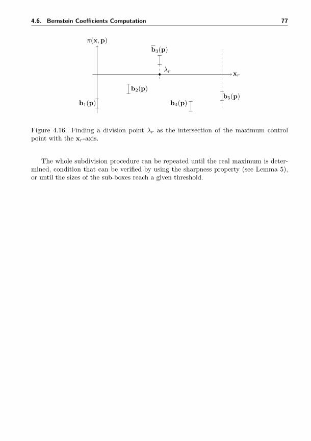
4.6. Bernstein Coefficients Computation 77
xr
π(x,p)
b1(p)
b2(p)
b3(p)
b4(p)b5(p)
λr
Figure 4.16: Finding a division point λr as the intersection of the maximum controlpoint with the xr-axis.
The whole subdivision procedure can be repeated until the real maximum is deter-mined, condition that can be verified by using the sharpness property (see Lemma 5),or until the sizes of the sub-boxes reach a given threshold.

5Parameter Synthesis
In this chapter we focus on the parameter synthesis problem, that is, given a dynamicalsystem S = (X ,P, f), a set of initial conditions X0 ⊆ X , a parameter set P ⊆ P, anda specification ϕ, find the largest subset Pϕ ⊆ P such that for all x0 ∈ X0 and p ∈ P ,the trajectories ξpx0
of S satisfy the specification ϕ. In this work we assume that thespecifications are given as formulas of the Signal Temporal Logic (STL), a logic thatallows one to specify properties on dense-time real-valued functions.
STL and its standard semantics will be presented in Section 5.1. In order to adaptSTL to our parameter synthesis context, in Section 5.2 we will define a new semantics,called synthesis semantics, to reason on flowpipes and sets of parameters rather than onsingle trajectories. In Section 5.3 we will present a synthesis algorithm that can be usedto solve the parameter synthesis problem for discrete-time dynamical systems and STLspecifications. Its correctness and complexity will be discussed in Section 5.3.4. Finally,in Section 5.4, also exploiting the reachability techniques developed in Chapter 4, wewill focus on the implementation of our synthesis algorithm in the case of discrete-timepolynomial dynamical systems.
5.1 Signal Temporal Logic
Temporal logic [163] is a formalism used to specify and reason on properties that involvetime. It is typically adopted in the context of formal verification, where a temporal logicformula specifies the acceptable behaviors of a system and an algorithm is used to checkwhether all the behaviors of the system satisfy the formula. This procedure is commonlyknown as model checking [46]. Recently, temporal logic has found applications outsideformal verification, for instance in monitoring. In this case, a formal model is notnecessary, since the system can be treated as a black box whose observable behaviorscan be monitored by evaluating the satisfaction level of the desired temporal property.
Signal Temporal Logic (STL [143, 144]) is a recent logic that allows one to specifyproperties of dense-time real-valued signals. It is particularly suitable for monitoringblackbox systems, such as industrial models (see, e.g., [116, 115]) and biological systems(see, e.g., [68, 177]). It has also been used in the study of parametric systems, (see,
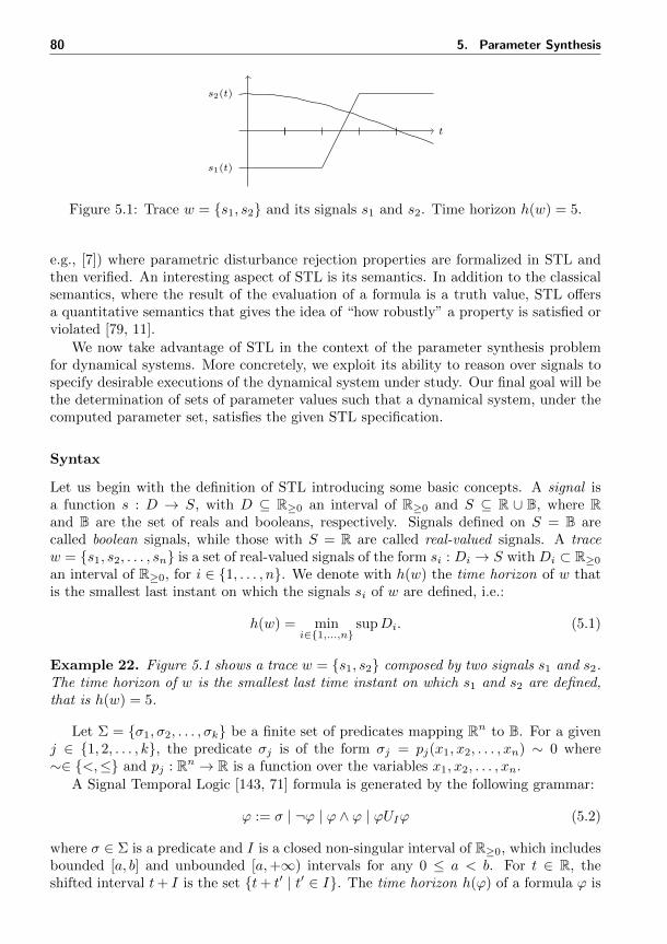
80 5. Parameter Synthesis
t
s1(t)
s2(t)
Figure 5.1: Trace w = s1, s2 and its signals s1 and s2. Time horizon h(w) = 5.
e.g., [7]) where parametric disturbance rejection properties are formalized in STL andthen verified. An interesting aspect of STL is its semantics. In addition to the classicalsemantics, where the result of the evaluation of a formula is a truth value, STL offersa quantitative semantics that gives the idea of “how robustly” a property is satisfied orviolated [79, 11].
We now take advantage of STL in the context of the parameter synthesis problemfor dynamical systems. More concretely, we exploit its ability to reason over signals tospecify desirable executions of the dynamical system under study. Our final goal will bethe determination of sets of parameter values such that a dynamical system, under thecomputed parameter set, satisfies the given STL specification.
Syntax
Let us begin with the definition of STL introducing some basic concepts. A signal isa function s : D → S, with D ⊆ R≥0 an interval of R≥0 and S ⊆ R ∪ B, where Rand B are the set of reals and booleans, respectively. Signals defined on S = B arecalled boolean signals, while those with S = R are called real-valued signals. A tracew = s1, s2, . . . , sn is a set of real-valued signals of the form si : Di → S with Di ⊂ R≥0an interval of R≥0, for i ∈ 1, . . . , n. We denote with h(w) the time horizon of w thatis the smallest last instant on which the signals si of w are defined, i.e.:
h(w) = mini∈1,...,n
supDi. (5.1)
Example 22. Figure 5.1 shows a trace w = s1, s2 composed by two signals s1 and s2.The time horizon of w is the smallest last time instant on which s1 and s2 are defined,that is h(w) = 5.
Let Σ = σ1, σ2, . . . , σk be a finite set of predicates mapping Rn to B. For a givenj ∈ 1, 2, . . . , k, the predicate σj is of the form σj = pj(x1, x2, . . . , xn) ∼ 0 where∼∈ <,≤ and pj : Rn → R is a function over the variables x1, x2, . . . , xn.
A Signal Temporal Logic [143, 71] formula is generated by the following grammar:
ϕ := σ | ¬ϕ | ϕ ∧ ϕ | ϕUIϕ (5.2)
where σ ∈ Σ is a predicate and I is a closed non-singular interval of R≥0, which includesbounded [a, b] and unbounded [a,+∞) intervals for any 0 ≤ a < b. For t ∈ R, theshifted interval t+ I is the set t+ t′ | t′ ∈ I. The time horizon h(ϕ) of a formula ϕ is
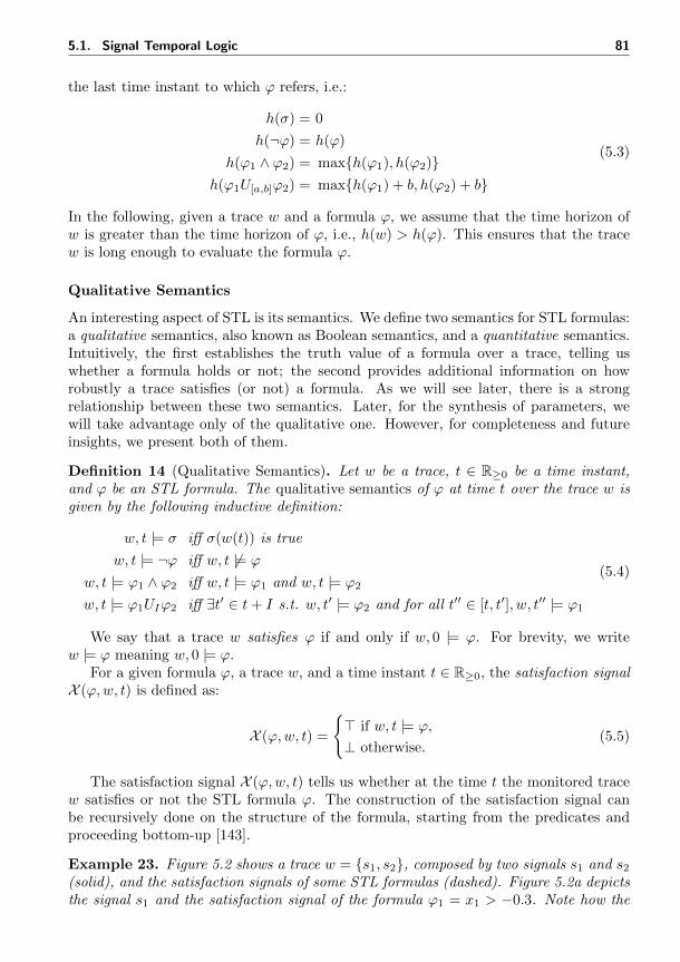
5.1. Signal Temporal Logic 81
the last time instant to which ϕ refers, i.e.:
h(σ) = 0
h(¬ϕ) = h(ϕ)
h(ϕ1 ∧ ϕ2) = maxh(ϕ1), h(ϕ2)h(ϕ1U[a,b]ϕ2) = maxh(ϕ1) + b, h(ϕ2) + b
(5.3)
In the following, given a trace w and a formula ϕ, we assume that the time horizon ofw is greater than the time horizon of ϕ, i.e., h(w) > h(ϕ). This ensures that the tracew is long enough to evaluate the formula ϕ.
Qualitative Semantics
An interesting aspect of STL is its semantics. We define two semantics for STL formulas:a qualitative semantics, also known as Boolean semantics, and a quantitative semantics.Intuitively, the first establishes the truth value of a formula over a trace, telling uswhether a formula holds or not; the second provides additional information on howrobustly a trace satisfies (or not) a formula. As we will see later, there is a strongrelationship between these two semantics. Later, for the synthesis of parameters, wewill take advantage only of the qualitative one. However, for completeness and futureinsights, we present both of them.
Definition 14 (Qualitative Semantics). Let w be a trace, t ∈ R≥0 be a time instant,and ϕ be an STL formula. The qualitative semantics of ϕ at time t over the trace w isgiven by the following inductive definition:
w, t |= σ iff σ(w(t)) is true
w, t |= ¬ϕ iff w, t 6|= ϕ
w, t |= ϕ1 ∧ ϕ2 iff w, t |= ϕ1 and w, t |= ϕ2
w, t |= ϕ1UIϕ2 iff ∃t′ ∈ t+ I s.t. w, t′ |= ϕ2 and for all t′′ ∈ [t, t′], w, t′′ |= ϕ1
(5.4)
We say that a trace w satisfies ϕ if and only if w, 0 |= ϕ. For brevity, we writew |= ϕ meaning w, 0 |= ϕ.
For a given formula ϕ, a trace w, and a time instant t ∈ R≥0, the satisfaction signalX (ϕ,w, t) is defined as:
X (ϕ,w, t) =
> if w, t |= ϕ,
⊥ otherwise.(5.5)
The satisfaction signal X (ϕ,w, t) tells us whether at the time t the monitored tracew satisfies or not the STL formula ϕ. The construction of the satisfaction signal canbe recursively done on the structure of the formula, starting from the predicates andproceeding bottom-up [143].
Example 23. Figure 5.2 shows a trace w = s1, s2, composed by two signals s1 and s2(solid), and the satisfaction signals of some STL formulas (dashed). Figure 5.2a depictsthe signal s1 and the satisfaction signal of the formula ϕ1 = x1 > −0.3. Note how the
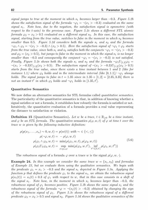
82 5. Parameter Synthesis
signal jumps to true at the moment in which s1 becomes larger than −0.3. Figure 5.2bshows the satisfaction signal of the formula ¬ϕ1 = ¬(x1 > −0.3) evaluated on the samesignal s1. Note how, due to the negation, the satisfaction signal is symmetric (withrespect to the t-axis) to the previous case. Figure 5.2c shows a different STL atomicformula ϕ2 = x2 > 0.5 evaluated on a different signal s2. In this case, the satisfactionsignal, starting from the true value, switches to false in the moment in which s2 becomessmaller than 0.5. Figure 5.2d considers both the signals s1 and s2 and the formula¬ϕ1 ∧ ϕ2 = ¬(x1 > −0.3) ∧ (x2 > 0.5). Here the satisfaction signal of ¬ϕ1 ∧ ϕ2 startsfrom the true value, since both s1 and s2 satisfies both the conjuncts ¬ϕ1 = ¬(x1 > −0.3)and ϕ2 = (x2 > 0.5), but jumps to false in the moment in which the signal s1 is no longersmaller than −0.3 and consequently the conjunct ¬ϕ1 = ¬(x1 > −0.3) is not satisfied.Finally, Figure 5.2e shows both the signals s1 and s2 and the formula ¬ϕ1U[1,2]ϕ2 =¬(x1 > −0.3)U[1,2](x2 > 0.5). The satisfaction signal of ¬(x1 > −0.3)U[1,2](x2 > 0.5)starts from the true value, since there exists a time instant between 1 and 2 (like forinstance 1.1) where ϕ2 holds and in the intermediate interval (like [0, 1.1]) ¬ϕ1 alwaysholds. The signal jumps to false in t = 1.35 since in 1.35 + [1, 2] = [2.35, 3.35] there isnot an instant t′ in which ϕ2 holds and ¬ϕ1 holds in [1.35, t′].
Quantitative Semantics
We now define an alternative semantics for STL formulas called quantitative semantics.The particularity of the quantitative semantics is that, in addition of knowing whether asignal satisfies or not a formula, it establishes how robustly the formula is satisfied or not.Intuitively, the quantitative evaluation of a formula provides a real value representingthe distance to satisfaction or violation.
Definition 15 (Quantitative Semantics). Let w be a trace, t ∈ R≥0 be a time instant,and ϕ be an STL formula. The quantitative semantics ρ(ϕ,w, t) of ϕ at time t over thetrace w is given by the following inductive definition:
ρ(p(x1, . . . , xn) ∼ 0, w, t) = p(w(t)) with ∼ ∈ <,≤ρ(¬ϕ,w, t) = − ρ(ϕ,w, t)
ρ(ϕ1 ∧ ϕ2, w, t) = min(ρ(ϕ1, w, t), ρ(ϕ2, w, t))
ρ(ϕ1UIϕ2, w, t) = supt′∈t+I
min(ρ(ϕ2, w, t′), inf
t′′∈[t,t′]ρ(ϕ1, w, t
′′))
(5.6)
The robustness signal of a formula ϕ over a trace w is the signal ρ(ϕ,w, ·).
Example 24. In this example we consider the same trace w = s1, s2 and formulasof Example 23, but we evaluate them using the qualitative semantics. We begin withthe predicate ϕ1 = x1 > −0.3 and the signal s1 depicted in Figure 5.3a. Applying thefunction p that defines the predicate ϕ1 to the signal s1, we obtain the robustness signalp(s1(t)) = s1(t) + 0.3 of ϕ1 with respect to w, that in this case consists in a shift ofthe signal s1. Note how, in the moment in which s1 becomes larger than −0.3, therobustness signal of ϕ1 becomes positive. Figure 5.3b shows the same signal s1 and therobustness signal of the formula ¬ϕ = ¬(s1(t) > −0.3) obtained by changing the signof the robustness signal of ϕ1. Figure 5.3c shows the robustness signal of a differentpredicate ϕ2 = x2 > 0.5 and signal s2. Figure 5.3d shows the qualitative semantics of the
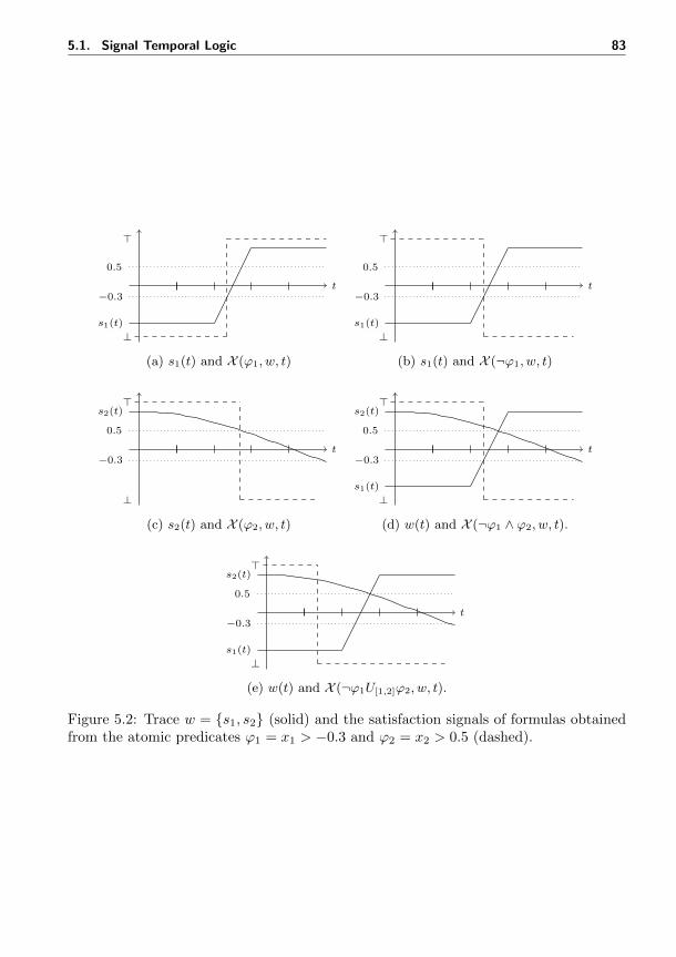
5.1. Signal Temporal Logic 83
t
s1(t)
0.5
−0.3
>
⊥
(a) s1(t) and X (ϕ1, w, t)
t
s1(t)
0.5
−0.3
>
⊥
(b) s1(t) and X (¬ϕ1, w, t)
t
s2(t)
0.5
−0.3
>
⊥
(c) s2(t) and X (ϕ2, w, t)
t
s1(t)
s2(t)
0.5
−0.3
>
⊥
(d) w(t) and X (¬ϕ1 ∧ ϕ2, w, t).
t
s1(t)
s2(t)
0.5
−0.3
>
⊥
(e) w(t) and X (¬ϕ1U[1,2]ϕ2, w, t).
Figure 5.2: Trace w = s1, s2 (solid) and the satisfaction signals of formulas obtainedfrom the atomic predicates ϕ1 = x1 > −0.3 and ϕ2 = x2 > 0.5 (dashed).
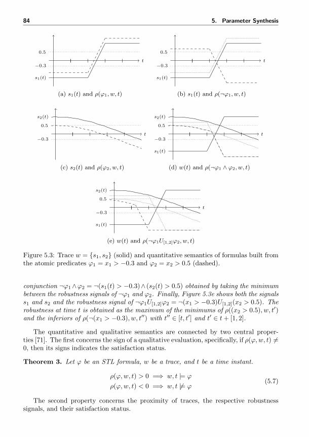
84 5. Parameter Synthesis
t
s1(t)
0.5
−0.3
(a) s1(t) and ρ(ϕ1, w, t)
t
s1(t)
0.5
−0.3
(b) s1(t) and ρ(¬ϕ1, w, t)
t
s2(t)
0.5
−0.3
(c) s2(t) and ρ(ϕ2, w, t)
t
s1(t)
s2(t)
0.5
−0.3
(d) w(t) and ρ(¬ϕ1 ∧ ϕ2, w, t)
t
s1(t)
s2(t)
0.5
−0.3
(e) w(t) and ρ(¬ϕ1U[1,2]ϕ2, w, t)
Figure 5.3: Trace w = s1, s2 (solid) and quantitative semantics of formulas built fromthe atomic predicates ϕ1 = x1 > −0.3 and ϕ2 = x2 > 0.5 (dashed).
conjunction ¬ϕ1∧ϕ2 = ¬(s1(t) > −0.3)∧ (s2(t) > 0.5) obtained by taking the minimumbetween the robustness signals of ¬ϕ1 and ϕ2. Finally, Figure 5.3e shows both the signalss1 and s2 and the robustness signal of ¬ϕ1U[1,2]ϕ2 = ¬(x1 > −0.3)U[1,2](x2 > 0.5). Therobustness at time t is obtained as the maximum of the minimums of ρ((x2 > 0.5), w, t′)and the inferiors of ρ(¬(x1 > −0.3), w, t′′) with t′′ ∈ [t, t′] and t′ ∈ t+ [1, 2].
The quantitative and qualitative semantics are connected by two central proper-ties [71]. The first concerns the sign of a qualitative evaluation, specifically, if ρ(ϕ,w, t) 6=0, then its signs indicates the satisfaction status.
Theorem 3. Let ϕ be an STL formula, w be a trace, and t be a time instant.
ρ(ϕ,w, t) > 0 =⇒ w, t |= ϕ
ρ(ϕ,w, t) < 0 =⇒ w, t 6|= ϕ(5.7)
The second property concerns the proximity of traces, the respective robustnesssignals, and their satisfaction status.
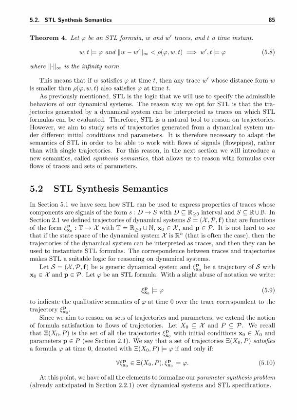
5.2. STL Synthesis Semantics 85
Theorem 4. Let ϕ be an STL formula, w and w′ traces, and t a time instant.
w, t |= ϕ and ‖w − w′‖∞ < ρ(ϕ,w, t) =⇒ w′, t |= ϕ (5.8)
where ‖·‖∞ is the infinity norm.
This means that if w satisfies ϕ at time t, then any trace w′ whose distance form wis smaller then ρ(ϕ,w, t) also satisfies ϕ at time t.
As previously mentioned, STL is the logic that we will use to specify the admissiblebehaviors of our dynamical systems. The reason why we opt for STL is that the tra-jectories generated by a dynamical system can be interpreted as traces on which STLformulas can be evaluated. Therefore, STL is a natural tool to reason on trajectories.However, we aim to study sets of trajectories generated from a dynamical system un-der different initial conditions and parameters. It is therefore necessary to adapt thesemantics of STL in order to be able to work with flows of signals (flowpipes), ratherthan with single trajectories. For this reason, in the next section we will introduce anew semantics, called synthesis semantics, that allows us to reason with formulas overflows of traces and sets of parameters.
5.2 STL Synthesis Semantics
In Section 5.1 we have seen how STL can be used to express properties of traces whosecomponents are signals of the form s : D → S with D ⊆ R≥0 interval and S ⊆ R∪B. InSection 2.1 we defined trajectories of dynamical systems S = (X ,P, f) that are functionsof the form ξpx0
: T → X with T = R≥0 ∪ N, x0 ∈ X , and p ∈ P. It is not hard to seethat if the state space of the dynamical system X is Rn (that is often the case), then thetrajectories of the dynamical system can be interpreted as traces, and then they can beused to instantiate STL formulas. The correspondence between traces and trajectoriesmakes STL a suitable logic for reasoning on dynamical systems.
Let S = (X ,P, f) be a generic dynamical system and ξpx0be a trajectory of S with
x0 ∈ X and p ∈ P. Let ϕ be an STL formula. With a slight abuse of notation we write:
ξpx0|= ϕ (5.9)
to indicate the qualitative semantics of ϕ at time 0 over the trace correspondent to thetrajectory ξpx0
.
Since we aim to reason on sets of trajectories and parameters, we extend the notionof formula satisfaction to flows of trajectories. Let X0 ⊆ X and P ⊆ P. We recallthat Ξ(X0, P ) is the set of all the trajectories ξpx0
with initial conditions x0 ∈ X0 andparameters p ∈ P (see Section 2.1). We say that a set of trajectories Ξ(X0, P ) satisfiesa formula ϕ at time 0, denoted with Ξ(X0, P ) |= ϕ if and only if:
∀ξpx0∈ Ξ(X0, P ), ξpx0
|= ϕ. (5.10)
At this point, we have of all the elements to formalize our parameter synthesis problem(already anticipated in Section 2.2.1) over dynamical systems and STL specifications.
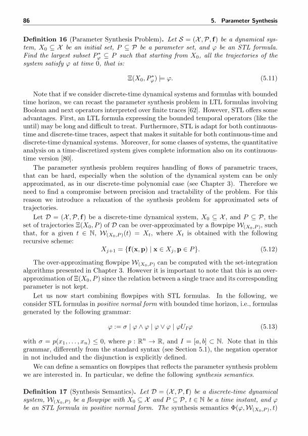
86 5. Parameter Synthesis
Definition 16 (Parameter Synthesis Problem). Let S = (X ,P, f) be a dynamical sys-tem, X0 ⊆ X be an initial set, P ⊆ P be a parameter set, and ϕ be an STL formula.Find the largest subset P ∗ϕ ⊆ P such that starting from X0, all the trajectories of thesystem satisfy ϕ at time 0, that is:
Ξ(X0, P∗ϕ) |= ϕ. (5.11)
Note that if we consider discrete-time dynamical systems and formulas with boundedtime horizon, we can recast the parameter synthesis problem in LTL formulas involvingBoolean and next operators interpreted over finite traces [62]. However, STL offers someadvantages. First, an LTL formula expressing the bounded temporal operators (like theuntil) may be long and difficult to treat. Furthermore, STL is adapt for both continuous-time and discrete-time traces, aspect that makes it suitable for both continuous-time anddiscrete-time dynamical systems. Moreover, for some classes of systems, the quantitativeanalysis on a time-discretized system gives complete information also on its continuous-time version [80].
The parameter synthesis problem requires handling of flows of parametric traces,that can be hard, especially when the solution of the dynamical system can be onlyapproximated, as in our discrete-time polynomial case (see Chapter 3). Therefore weneed to find a compromise between precision and tractability of the problem. For thisreason we introduce a relaxation of the synthesis problem for approximated sets oftrajectories.
Let D = (X ,P, f) be a discrete-time dynamical system, X0 ⊆ X , and P ⊆ P, theset of trajectories Ξ(X0, P ) of D can be over-approximated by a flowpipe W(X0,P ), suchthat, for a given t ∈ N, W(X0,P )(t) = Xt, where Xt is obtained with the followingrecursive scheme:
Xj+1 = f(x,p) | x ∈ Xj ,p ∈ P. (5.12)
The over-approximating flowpipe W(X0,P ) can be computed with the set-integrationalgorithms presented in Chapter 3. However it is important to note that this is an over-approximation of Ξ(X0, P ) since the relation between a single trace and its correspondingparameter is not kept.
Let us now start combining flowpipes with STL formulas. In the following, weconsider STL formulas in positive normal form with bounded time horizon, i.e., formulasgenerated by the following grammar:
ϕ := σ | ϕ ∧ ϕ | ϕ ∨ ϕ | ϕUIϕ (5.13)
with σ = p(x1, . . . , xn) ≤ 0, where p : Rn → R, and I = [a, b] ⊂ N. Note that in thisgrammar, differently from the standard syntax (see Section 5.1), the negation operatorin not included and the disjunction is explicitly defined.
We can define a semantics on flowpipes that reflects the parameter synthesis problemwe are interested in. In particular, we define the following synthesis semantics.
Definition 17 (Synthesis Semantics). Let D = (X ,P, f) be a discrete-time dynamicalsystem, W(X0,P ) be a flowpipe with X0 ⊆ X and P ⊆ P, t ∈ N be a time instant, and ϕbe an STL formula in positive normal form. The synthesis semantics Φ(ϕ,W(X0,P ), t)
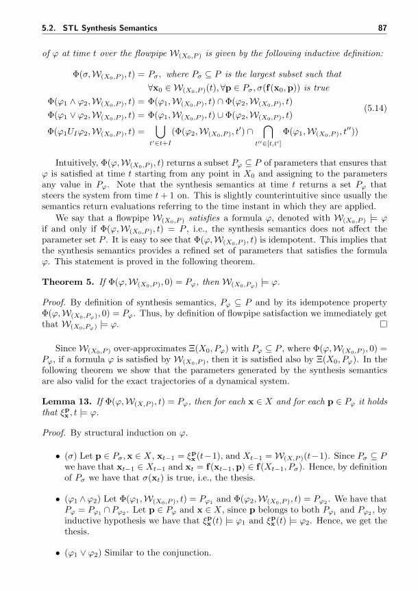
5.2. STL Synthesis Semantics 87
of ϕ at time t over the flowpipe W(X0,P ) is given by the following inductive definition:
Φ(σ,W(X0,P ), t) = Pσ, where Pσ ⊆ P is the largest subset such that
∀x0 ∈ W(X0,P )(t),∀p ∈ Pσ, σ(f(x0,p)) is true
Φ(ϕ1 ∧ ϕ2,W(X0,P ), t) = Φ(ϕ1,W(X0,P ), t) ∩ Φ(ϕ2,W(X0,P ), t)
Φ(ϕ1 ∨ ϕ2,W(X0,P ), t) = Φ(ϕ1,W(X0,P ), t) ∪ Φ(ϕ2,W(X0,P ), t)
Φ(ϕ1UIϕ2,W(X0,P ), t) =⋃
t′∈t+I(Φ(ϕ2,W(X0,P ), t
′) ∩⋂
t′′∈[t,t′]
Φ(ϕ1,W(X0,P ), t′′))
(5.14)
Intuitively, Φ(ϕ,W(X0,P ), t) returns a subset Pϕ ⊆ P of parameters that ensures thatϕ is satisfied at time t starting from any point in X0 and assigning to the parametersany value in Pϕ. Note that the synthesis semantics at time t returns a set Pϕ thatsteers the system from time t+ 1 on. This is slightly counterintuitive since usually thesemantics return evaluations referring to the time instant in which they are applied.
We say that a flowpipe W(X0,P ) satisfies a formula ϕ, denoted with W(X0,P ) |= ϕif and only if Φ(ϕ,W(X0,P ), t) = P , i.e., the synthesis semantics does not affect theparameter set P . It is easy to see that Φ(ϕ,W(X0,P ), t) is idempotent. This implies thatthe synthesis semantics provides a refined set of parameters that satisfies the formulaϕ. This statement is proved in the following theorem.
Theorem 5. If Φ(ϕ,W(X0,P ), 0) = Pϕ, then W(X0,Pϕ) |= ϕ.
Proof. By definition of synthesis semantics, Pϕ ⊆ P and by its idempotence propertyΦ(ϕ,W(X0,Pϕ), 0) = Pϕ. Thus, by definition of flowpipe satisfaction we immediately getthat W(X0,Pϕ) |= ϕ.
SinceW(X0,P ) over-approximates Ξ(X0, Pϕ) with Pϕ ⊆ P , where Φ(ϕ,W(X0,P ), 0) =Pϕ, if a formula ϕ is satisfied by W(X0,P ), then it is satisfied also by Ξ(X0, Pϕ). In thefollowing theorem we show that the parameters generated by the synthesis semanticsare also valid for the exact trajectories of a dynamical system.
Lemma 13. If Φ(ϕ,W(X,P ), t) = Pϕ, then for each x ∈ X and for each p ∈ Pϕ it holdsthat ξpx , t |= ϕ.
Proof. By structural induction on ϕ.
• (σ) Let p ∈ Pσ,x ∈ X, xt−1 = ξpx (t−1), and Xt−1 =W(X,P )(t−1). Since Pσ ⊆ Pwe have that xt−1 ∈ Xt−1 and xt = f(xt−1,p) ∈ f(Xt−1, Pσ). Hence, by definitionof Pσ we have that σ(xt) is true, i.e., the thesis.
• (ϕ1 ∧ϕ2) Let Φ(ϕ1,W(X0,P ), t) = Pϕ1 and Φ(ϕ2,W(X0,P ), t) = Pϕ2 . We have thatPϕ = Pϕ1 ∩Pϕ2 . Let p ∈ Pϕ and x ∈ X, since p belongs to both Pϕ1 and Pϕ2 , byinductive hypothesis we have that ξpx (t) |= ϕ1 and ξpx (t) |= ϕ2. Hence, we get thethesis.
• (ϕ1 ∨ ϕ2) Similar to the conjunction.
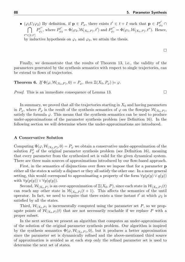
88 5. Parameter Synthesis
• (ϕ1UIϕ2) By definition, if p ∈ Pϕ, there exists t′ ∈ t + I such that p ∈ P t′
ϕ2∩⋂
t′′∈[t,t′]
P t′′
ϕ1, where P t
′
ϕ2= Φ(ϕ2,W(X0,P ), t
′) and P t′′
ϕ1= Φ(ϕ1,W(X0,P ), t
′′). Hence,
by inductive hypothesis on ϕ1 and ϕ2, we attain the thesis.
Finally, we demonstrate that the results of Theorem 13, i.e., the validity of theparameters generated by the synthesis semantics with respect to single trajectories, canbe extend to flows of trajectories.
Theorem 6. If Φ(ϕ,W(X0,P ), 0) = Pϕ, then Ξ(X0, Pϕ) |= ϕ.
Proof. This is an immediate consequence of Lemma 13.
In summary, we proved that all the trajectories starting in X0 and having parametersin Pϕ, where Pϕ is the result of the synthesis semantics of ϕ on the flowpipe W(X0,P ),satisfy the formula ϕ. This means that the synthesis semantics can be used to produceunder-approximations of the parameter synthesis problem (see Definition 16). In thefollowing section we will determine where the under-approximations are introduced.
A Conservative Solution
Computing Φ(ϕ,W(X0,P ), 0) = Pϕ we obtain a conservative under-approximation of thesolution P ∗ϕ of the original parameter synthesis problem (see Definition 16), meaningthat every parameter from the synthesized set is valid for the given dynamical system.There are three main sources of approximations introduced by our flow-based approach.
First, in the semantics of disjunctions over flows we impose that for a parameter peither all the states x satisfy a disjunct or they all satisfy the other one. In a more generalsetting, this would correspond to approximating a property of the form ∀y(p(y) ∨ q(y))with ∀y(p(y)) ∨ ∀y(q(y)).
Second,W(X0,P ) is an over-approximation of Ξ(X0, P ), since each state inW(X0,P )(t)can reach any other state in W(X0,P )(t + 1). This affects the semantics of the untiloperator. In fact, we need to require that there exists a time instant t′ at which ϕ2 issatisfied by all the states.
Third, W(X0,P ) is incrementally computed using the parameter set P , so we prop-agate points of W(X0,P )(t) that are not necessarily reachable if we replace P with aproper subset.
In the next section we present an algorithm that computes an under-approximationof the solution of the original parameter synthesis problem. Our algorithm is inspiredby the synthesis semantics Φ(ϕ,W(X0,P ), 0), but it produces a better approximationsince the parameter set is dynamically refined and the above-mentioned third sourceof approximation is avoided as at each step only the refined parameter set is used todetermine the next set of states.
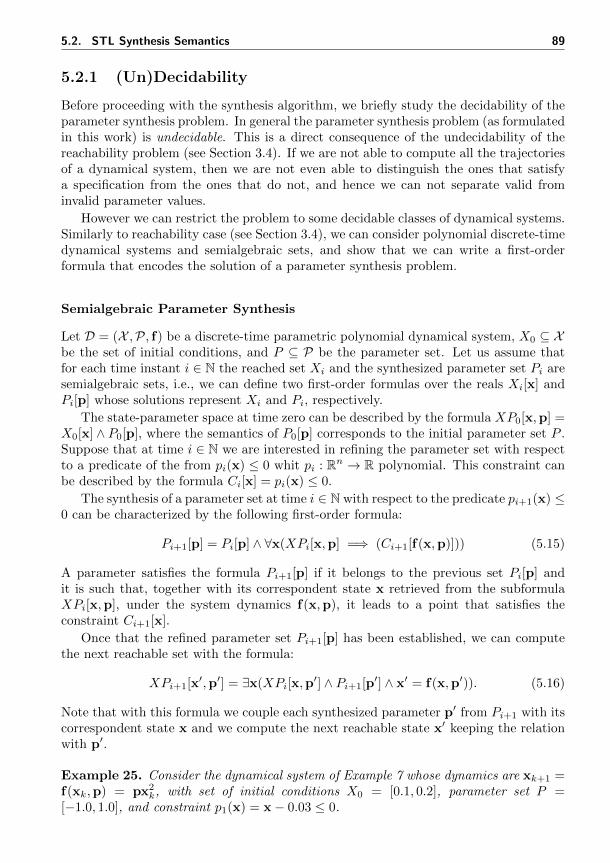
5.2. STL Synthesis Semantics 89
5.2.1 (Un)Decidability
Before proceeding with the synthesis algorithm, we briefly study the decidability of theparameter synthesis problem. In general the parameter synthesis problem (as formulatedin this work) is undecidable. This is a direct consequence of the undecidability of thereachability problem (see Section 3.4). If we are not able to compute all the trajectoriesof a dynamical system, then we are not even able to distinguish the ones that satisfya specification from the ones that do not, and hence we can not separate valid frominvalid parameter values.
However we can restrict the problem to some decidable classes of dynamical systems.Similarly to reachability case (see Section 3.4), we can consider polynomial discrete-timedynamical systems and semialgebraic sets, and show that we can write a first-orderformula that encodes the solution of a parameter synthesis problem.
Semialgebraic Parameter Synthesis
Let D = (X ,P, f) be a discrete-time parametric polynomial dynamical system, X0 ⊆ Xbe the set of initial conditions, and P ⊆ P be the parameter set. Let us assume thatfor each time instant i ∈ N the reached set Xi and the synthesized parameter set Pi aresemialgebraic sets, i.e., we can define two first-order formulas over the reals Xi[x] andPi[p] whose solutions represent Xi and Pi, respectively.
The state-parameter space at time zero can be described by the formula XP0[x,p] =X0[x] ∧ P0[p], where the semantics of P0[p] corresponds to the initial parameter set P .Suppose that at time i ∈ N we are interested in refining the parameter set with respectto a predicate of the from pi(x) ≤ 0 whit pi : Rn → R polynomial. This constraint canbe described by the formula Ci[x] = pi(x) ≤ 0.
The synthesis of a parameter set at time i ∈ N with respect to the predicate pi+1(x) ≤0 can be characterized by the following first-order formula:
Pi+1[p] = Pi[p] ∧ ∀x(XPi[x,p] =⇒ (Ci+1[f(x,p)])) (5.15)
A parameter satisfies the formula Pi+1[p] if it belongs to the previous set Pi[p] andit is such that, together with its correspondent state x retrieved from the subformulaXPi[x,p], under the system dynamics f(x,p), it leads to a point that satisfies theconstraint Ci+1[x].
Once that the refined parameter set Pi+1[p] has been established, we can computethe next reachable set with the formula:
XPi+1[x′,p′] = ∃x(XPi[x,p′] ∧ Pi+1[p′] ∧ x′ = f(x,p′)). (5.16)
Note that with this formula we couple each synthesized parameter p′ from Pi+1 with itscorrespondent state x and we compute the next reachable state x′ keeping the relationwith p′.
Example 25. Consider the dynamical system of Example 7 whose dynamics are xk+1 =f(xk,p) = px2
k, with set of initial conditions X0 = [0.1, 0.2], parameter set P =[−1.0, 1.0], and constraint p1(x) = x− 0.03 ≤ 0.
90 5. Parameter Synthesis
The parameter and state-parameter sets at time zero can be described by the formulas:
P0[x0,p] ≡− 1.0 ≤ p ≤ 1.0
XP0[x0,p] ≡ 0.1 ≤ x0 ≤ 0.2 ∧ −1.0 ≤ p ≤ 1.0(5.17)
and the constraint by the formula:
C1[x] ≡ x− 0.03 ≤ 0. (5.18)
With this setting, the valid parameter set within a single step can be characterizedby the formula:
P1[p] ≡ P0[p] ∧ ∀x(XP0[x,p] =⇒ C1[f(x,p)])
≡ (−p− 1 ≤ 0 ∧ p− 1 ≤ 0) ∧ ∀x(((−10x + 1 ≤ 0 ∧ 5x− 1 ≤ 0)∧(−p− 1 ≤ 0 ∧ p− 1 ≤ 0)) =⇒ 100px2 − 3 ≤ 0)
(5.19)
whose equivalent version produced by the quantifier eliminator is:
P1[p] ≡ p + 1 ≥ 0 ∧ 4p− 3 ≤ 0. (5.20)
Thus, the refined parameter set is the set of points satisfying P1[p], i.e, Ps = [−1, 3/4].
Looking at the big picture, we can decompose an STL formula with bounded timehorizon in a finite series of checks on basic predicates (see the discussion between thecorrespondence of bounded discrete-time STL and LTL in Section 5.2). This meansthat the parameter synthesis, in this specific case, can be reduced to the satisfiability offirst-order formulas, a problem which is well known for being decidable [179, 47].
Unluckily, decidability does not imply feasibility. The quantifier elimination proce-dure, needed to establish the truth value of a first-oder formula over the reals, is doublyexponential in the degree of the functions appearing in the formula [102] (or in thenumber of quantifier alternations, depending on the algorithm). Thus, this approachshows that the problem is decidable and exactly solvable but it also points out that itis computationally costly. Hence, if we want to find valid parameter sets for nontrivialsystems, we need to develop an alternative technique.
5.3 Synthesis Algorithm
An intuitive way to solve our synthesis problem is to compute the reachable sets Xj
at each time instant j, up to a fixed time instant k ∈ N. Then, by examining thesets from time k back to time 0, we can derive the conditions on the parameters forthe satisfaction of the temporal property, as in the standard bottom-up monitoringapproaches [143]. In other terms, we could backwardly compute the synthesis semanticsof a formula with respect to a precomputed flowpipe. However, while in monitoring onlya single trace at a time is considered and that trace is already given, in our parametersynthesis problem the reachable set needs to be approximated (since exact reachabilitycomputation is often impossible). When approximations are used, a major drawback of
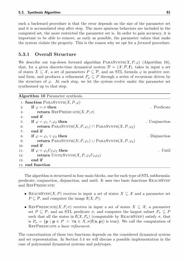
5.3. Synthesis Algorithm 91
such a backward procedure is that the error depends on the size of the parameter setand it is accumulated step after step. The more spurious behaviors are included in thecomputed set, the more restricted the parameter set is. In order to gain accuracy, it isimportant to be able to remove, as early as possible, the parameter values that makethe system violate the property. This is the reason why we opt for a forward procedure.
5.3.1 Overall Structure
We describe our top-down forward algorithm ParaSynth(X,P, ϕ) (Algorithm 10),that, for a given discrete-time dynamical system D = (X ,P, f), takes in input a setof states X ⊆ X , a set of parameters P ⊆ P, and an STL formula ϕ in positive nor-mal form, and produces a refinement Pϕ ⊆ P through a series of recursions driven bythe structure of ϕ. At each step, we let the system evolve under the parameter setsynthesized up to that step.
Algorithm 10 Parameter synthesis.
1: function ParaSynth(X,P, ϕ)2: if ϕ = σ then . Predicate3: return RefPredicate(X,P, σ)4: end if5: if ϕ = ϕ1 ∧ ϕ2 then . Conjunction6: return ParaSynth(X,P, ϕ1) ∩ ParaSynth(X,P, ϕ2)7: end if8: if ϕ = ϕ1 ∨ ϕ2 then . Disjunction9: return ParaSynth(X,P, ϕ1) ∪ ParaSynth(X,P, ϕ2)
10: end if11: if ϕ = ϕ1UIϕ2 then . Until12: return UntilSynth(X,P, ϕ1UIϕ2)13: end if14: end function
The algorithm is structured in four main blocks, one for each type of STL subformula:predicate, conjunction, disjunction, and until. It uses two basic functions ReachStepand RefPredicate:
• ReachStep(X,P ) receives in input a set of states X ⊆ X and a parameter setP ⊆ P, and computes the image f(X,P );
• RefPredicate(X,P, σ) receives in input a set of states X ⊆ X , a parameterset P ⊆ P, and an STL predicate σ, and computes the largest subset Pσ ⊆ Psuch that all the states in f(X,Pσ) (computable by ReachStep) satisfy σ, thatis Pσ = p | p ∈ P ∧ ∀x ∈ X,σ(f(x,p)) is true. We call the computation ofRefPredicate a basic refinement.
The concretization of these two functions depends on the considered dynamical systemand set representation. In Section 5.4 we will discuss a possible implementation in thecase of polynomial dynamical systems and polytopes.
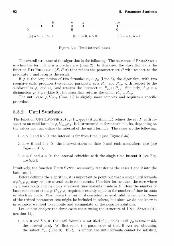
92 5. Parameter Synthesis
0
a b
(a) a > 0, b > 0
0
a b
(b) a = 0, b > 0
0
a, b
(c) a = 0, b = 0
Figure 5.4: Until interval cases.
The overall structure of the algorithm is the following. The base case of ParaSynthis when the formula ϕ is a predicate σ (Line 2). In this case, the algorithm calls thefunction RefPredicate(X,P, σ) that refines the parameter set P with respect to thepredicate σ and returns the result.
If ϕ is the conjunction of two formulas ϕ1 ∧ ϕ2 (Line 5), the algorithm, with tworecursive calls, produces two refined parameter sets Pϕ1
and Pϕ2, with respect to the
subformulas ϕ1 and ϕ2, and returns the intersection Pϕ1∩ Pϕ2
. Similarly, if ϕ is adisjunction ϕ1 ∨ ϕ2 (Line 8), the algorithm returns the union Pϕ1 ∪ Pϕ2 .
The until case ϕ1UIϕ2 (Line 11) is slightly more complex and requires a specificprocedure.
5.3.2 Until Synthesis
The function UntilSynth(X,P, ϕ1U[a,b]ϕ2) (Algorithm 11) refines the set P with re-spect to an until formula ϕ1U[a,b]ϕ2. It is structured in three main blocks, depending onthe values a, b that define the interval of the until formula. The cases are the following:
1. a > 0 and b > 0: the interval is far from time 0 (see Figure 5.4a);
2. a = 0 and b > 0: the interval starts at time 0 and ends somewhere else (seeFigure 5.4b);
3. a = 0 and b = 0: the interval coincides with the single time instant 0 (see Fig-ure 5.4c).
Intuitively, the function UntilSynth recursively transforms the cases 1 and 2 into thebase case 3.
Before defining the algorithm, it is important to point out that a single until formulaϕ1U[a,b]ϕ2 may require several basic refinements. Consider for instance the case whereϕ1 always holds and ϕ2 holds at several time instants inside [a, b]. Here the number ofbasic refinements that ϕ1U[a,b]ϕ2 requires is exactly equal to the number of time instantsin which ϕ2 holds. This means that an until can admit several valid refinements. Someof the refined parameter sets might be included in others, but since we do not know itin advance, we need to compute and accumulate all the possible solutions.
Let us now analyze the three cases constituting the structure of UntilSynth (Al-gorithm 11):
1. a > 0 and b > 0: the until formula is satisfied if ϕ1 holds until ϕ2 is true insidethe interval [a, b]. We first refine the parameters at time 0 over ϕ1, obtainingthe subset Pϕ1 (Line 3). If Pϕ1 is empty, the until formula cannot be satisfied,
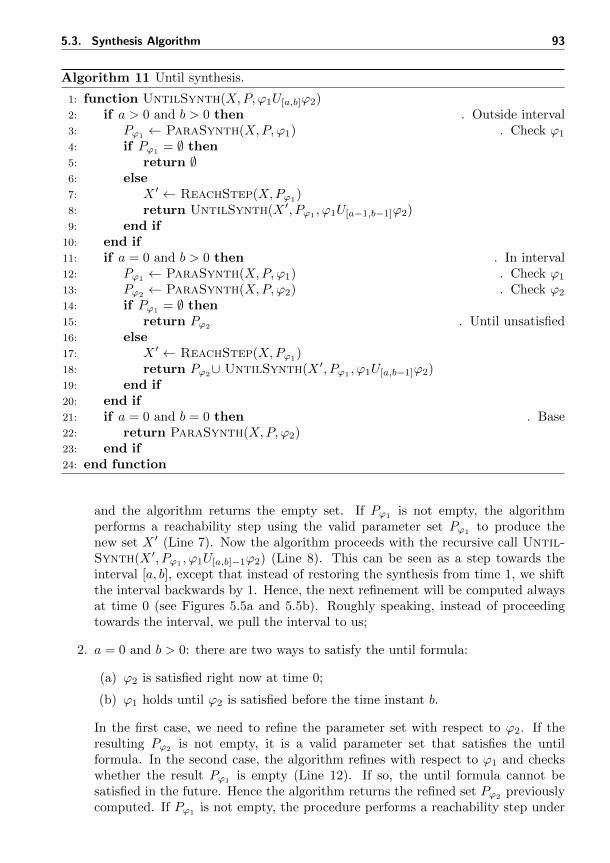
5.3. Synthesis Algorithm 93
Algorithm 11 Until synthesis.
1: function UntilSynth(X,P, ϕ1U[a,b]ϕ2)2: if a > 0 and b > 0 then . Outside interval3: Pϕ1 ← ParaSynth(X,P, ϕ1) . Check ϕ1
4: if Pϕ1 = ∅ then5: return ∅6: else7: X ′ ← ReachStep(X,Pϕ1
)8: return UntilSynth(X ′, Pϕ1 , ϕ1U[a−1,b−1]ϕ2)9: end if
10: end if11: if a = 0 and b > 0 then . In interval12: Pϕ1
← ParaSynth(X,P, ϕ1) . Check ϕ1
13: Pϕ2← ParaSynth(X,P, ϕ2) . Check ϕ2
14: if Pϕ1 = ∅ then15: return Pϕ2 . Until unsatisfied16: else17: X ′ ← ReachStep(X,Pϕ1
)18: return Pϕ2
∪ UntilSynth(X ′, Pϕ1, ϕ1U[a,b−1]ϕ2)
19: end if20: end if21: if a = 0 and b = 0 then . Base22: return ParaSynth(X,P, ϕ2)23: end if24: end function
and the algorithm returns the empty set. If Pϕ1 is not empty, the algorithmperforms a reachability step using the valid parameter set Pϕ1 to produce thenew set X ′ (Line 7). Now the algorithm proceeds with the recursive call Until-Synth(X ′, Pϕ1
, ϕ1U[a,b]−1ϕ2) (Line 8). This can be seen as a step towards theinterval [a, b], except that instead of restoring the synthesis from time 1, we shiftthe interval backwards by 1. Hence, the next refinement will be computed alwaysat time 0 (see Figures 5.5a and 5.5b). Roughly speaking, instead of proceedingtowards the interval, we pull the interval to us;
2. a = 0 and b > 0: there are two ways to satisfy the until formula:
(a) ϕ2 is satisfied right now at time 0;
(b) ϕ1 holds until ϕ2 is satisfied before the time instant b.
In the first case, we need to refine the parameter set with respect to ϕ2. If theresulting Pϕ2
is not empty, it is a valid parameter set that satisfies the untilformula. In the second case, the algorithm refines with respect to ϕ1 and checkswhether the result Pϕ1
is empty (Line 12). If so, the until formula cannot besatisfied in the future. Hence the algorithm returns the refined set Pϕ2 previouslycomputed. If Pϕ1 is not empty, the procedure performs a reachability step under
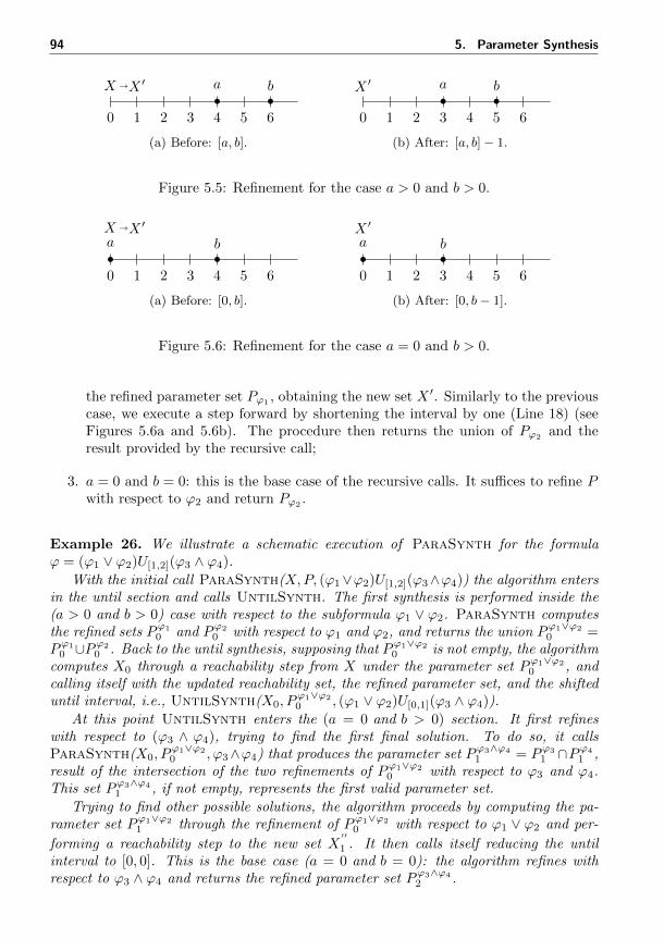
94 5. Parameter Synthesis
0 1 2 3 4 5 6
a bX →X ′
(a) Before: [a, b].
0 1 2 3 4 5 6
a bX ′
(b) After: [a, b]− 1.
Figure 5.5: Refinement for the case a > 0 and b > 0.
0 1 2 3 4 5 6
a bX →X ′
(a) Before: [0, b].
0 1 2 3 4 5 6
a bX ′
(b) After: [0, b− 1].
Figure 5.6: Refinement for the case a = 0 and b > 0.
the refined parameter set Pϕ1, obtaining the new set X ′. Similarly to the previous
case, we execute a step forward by shortening the interval by one (Line 18) (seeFigures 5.6a and 5.6b). The procedure then returns the union of Pϕ2
and theresult provided by the recursive call;
3. a = 0 and b = 0: this is the base case of the recursive calls. It suffices to refine Pwith respect to ϕ2 and return Pϕ2
.
Example 26. We illustrate a schematic execution of ParaSynth for the formulaϕ = (ϕ1 ∨ ϕ2)U[1,2](ϕ3 ∧ ϕ4).
With the initial call ParaSynth(X,P, (ϕ1∨ϕ2)U[1,2](ϕ3∧ϕ4)) the algorithm entersin the until section and calls UntilSynth. The first synthesis is performed inside the(a > 0 and b > 0) case with respect to the subformula ϕ1 ∨ ϕ2. ParaSynth computesthe refined sets Pϕ1
0 and Pϕ2
0 with respect to ϕ1 and ϕ2, and returns the union Pϕ1∨ϕ2
0 =Pϕ1
0 ∪Pϕ2
0 . Back to the until synthesis, supposing that Pϕ1∨ϕ2
0 is not empty, the algorithmcomputes X0 through a reachability step from X under the parameter set Pϕ1∨ϕ2
0 , andcalling itself with the updated reachability set, the refined parameter set, and the shifteduntil interval, i.e., UntilSynth(X0, P
ϕ1∨ϕ2
0 , (ϕ1 ∨ ϕ2)U[0,1](ϕ3 ∧ ϕ4)).
At this point UntilSynth enters the (a = 0 and b > 0) section. It first refineswith respect to (ϕ3 ∧ ϕ4), trying to find the first final solution. To do so, it callsParaSynth(X0, P
ϕ1∨ϕ2
0 , ϕ3∧ϕ4) that produces the parameter set Pϕ3∧ϕ4
1 = Pϕ3
1 ∩Pϕ4
1 ,result of the intersection of the two refinements of Pϕ1∨ϕ2
0 with respect to ϕ3 and ϕ4.This set Pϕ3∧ϕ4
1 , if not empty, represents the first valid parameter set.
Trying to find other possible solutions, the algorithm proceeds by computing the pa-rameter set Pϕ1∨ϕ2
1 through the refinement of Pϕ1∨ϕ2
0 with respect to ϕ1 ∨ ϕ2 and per-
forming a reachability step to the new set X′′
1 . It then calls itself reducing the untilinterval to [0, 0]. This is the base case (a = 0 and b = 0): the algorithm refines withrespect to ϕ3 ∧ ϕ4 and returns the refined parameter set Pϕ3∧ϕ4
2 .
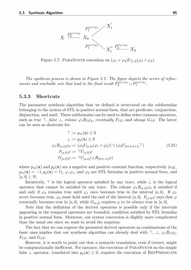
5.3. Synthesis Algorithm 95
X X0
X′
1
X′′
1 X2
Pϕ1∨ϕ2
0
Pϕ3∧ϕ4
1
Pϕ1∨ϕ2
1 Pϕ3∧ϕ4
2
Figure 5.7: ParaSynth execution on (ϕ1 ∨ ϕ2)U[1,2](ϕ3 ∧ ϕ4).
The synthesis process is shown in Figure 5.7. The figure depicts the series of refine-ments and reachable sets that lead to the final result Pϕ3∧ϕ4
2 ∪ Pϕ3∧ϕ4
1 .
5.3.3 Shortcuts
The parameter synthesis algorithm that we defined is structured on the subformulasbelonging to the syntax of STL in positive normal form, that are predicate, conjunction,disjunction, and until. These subformulas can be used to define other common operators,such as true >, false ⊥, release ϕ1RIϕ2, eventually FIϕ, and always GIϕ. The lattercan be seen as shortcuts for:
> := pm(x) ≤ 0
⊥ := pp(x) ≤ 0
ϕ1R[a,b]ϕ2 := (ϕ2U[a,b](ϕ1 ∧ ϕ2)) ∨ (ϕ2U[b+1,b+1]>)
F[a,b]ϕ := >U[a,b]ϕ
G[a,b]ϕ := >U[a,a](⊥R[0,b−a]ϕ)
(5.21)
where pm(x) and pp(x) are a negative and positive constant function, respectively (e.g.,pm(x) = −1, pp(x) = 1), ϕ,ϕ1, and ϕ2 are STL formulas in positive normal form, and[a, b] ⊂ N.
Intuitively, > is the logical operator satisfied by any trace, while ⊥ is the logicaloperator that cannot be satisfied by any trace. The release ϕ1R[a,b]ϕ2 is satisfied ifand only if ϕ2 remains true until ϕ1 once becomes true in the interval [a, b]. If ϕ1
never becomes true, ϕ2 must hold until the end of the interval [a, b]. F[a,b]ϕ says that ϕeventually becomes true in [a, b], while G[a,b] requires ϕ to be always true in [a, b].
Note that the definition of the derived operators is possible only if the intervalsappearing in the temporal operators are bounded, condition satisfied by STL formulasin positive normal form. Moreover, our syntax conversion is slightly more complicatedthan the usual one since we want to avoid the negation.
The fact that we can express the presented derived operators as combinations of thebasic ones implies that our synthesis algorithm can already deal with >, ⊥, ϕ1RIϕ2,FIϕ, and GIϕ.
However, it is worth to point out that a syntactic translation, even if correct, mightbe computationally inefficient. For instance, the execution of ParaSynth on the simplefalse ⊥ operator, translated into pp(x) ≤ 0, requires the execution of RefPredicate
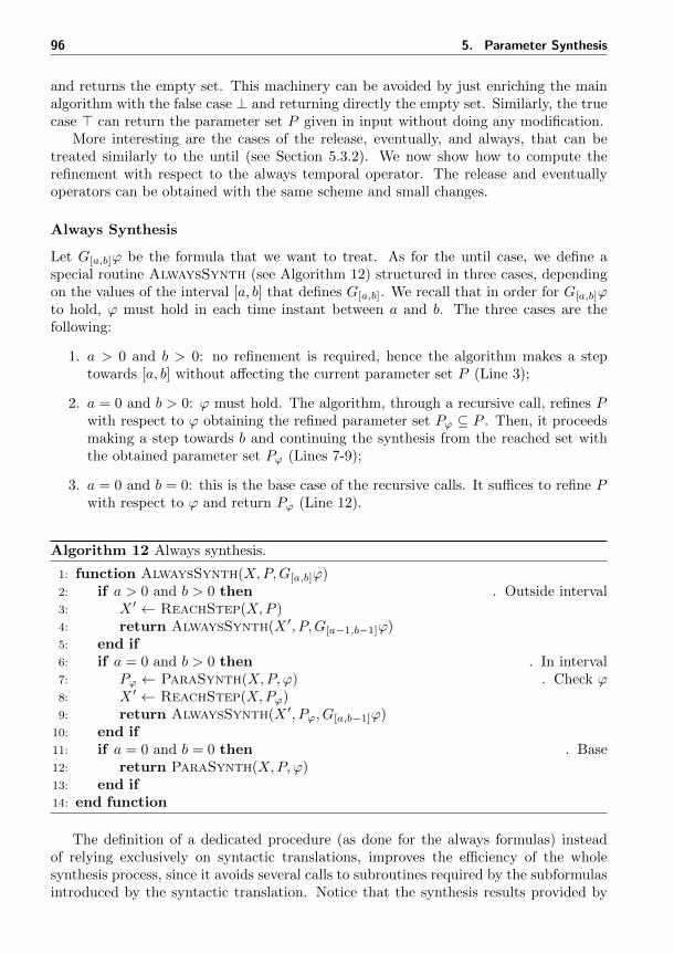
96 5. Parameter Synthesis
and returns the empty set. This machinery can be avoided by just enriching the mainalgorithm with the false case ⊥ and returning directly the empty set. Similarly, the truecase > can return the parameter set P given in input without doing any modification.
More interesting are the cases of the release, eventually, and always, that can betreated similarly to the until (see Section 5.3.2). We now show how to compute therefinement with respect to the always temporal operator. The release and eventuallyoperators can be obtained with the same scheme and small changes.
Always Synthesis
Let G[a,b]ϕ be the formula that we want to treat. As for the until case, we define aspecial routine AlwaysSynth (see Algorithm 12) structured in three cases, dependingon the values of the interval [a, b] that defines G[a,b]. We recall that in order for G[a,b]ϕto hold, ϕ must hold in each time instant between a and b. The three cases are thefollowing:
1. a > 0 and b > 0: no refinement is required, hence the algorithm makes a steptowards [a, b] without affecting the current parameter set P (Line 3);
2. a = 0 and b > 0: ϕ must hold. The algorithm, through a recursive call, refines Pwith respect to ϕ obtaining the refined parameter set Pϕ ⊆ P . Then, it proceedsmaking a step towards b and continuing the synthesis from the reached set withthe obtained parameter set Pϕ (Lines 7-9);
3. a = 0 and b = 0: this is the base case of the recursive calls. It suffices to refine Pwith respect to ϕ and return Pϕ (Line 12).
Algorithm 12 Always synthesis.
1: function AlwaysSynth(X,P,G[a,b]ϕ)2: if a > 0 and b > 0 then . Outside interval3: X ′ ← ReachStep(X,P )4: return AlwaysSynth(X ′, P,G[a−1,b−1]ϕ)5: end if6: if a = 0 and b > 0 then . In interval7: Pϕ ← ParaSynth(X,P, ϕ) . Check ϕ8: X ′ ← ReachStep(X,Pϕ)9: return AlwaysSynth(X ′, Pϕ, G[a,b−1]ϕ)
10: end if11: if a = 0 and b = 0 then . Base12: return ParaSynth(X,P, ϕ)13: end if14: end function
The definition of a dedicated procedure (as done for the always formulas) insteadof relying exclusively on syntactic translations, improves the efficiency of the wholesynthesis process, since it avoids several calls to subroutines required by the subformulasintroduced by the syntactic translation. Notice that the synthesis results provided by
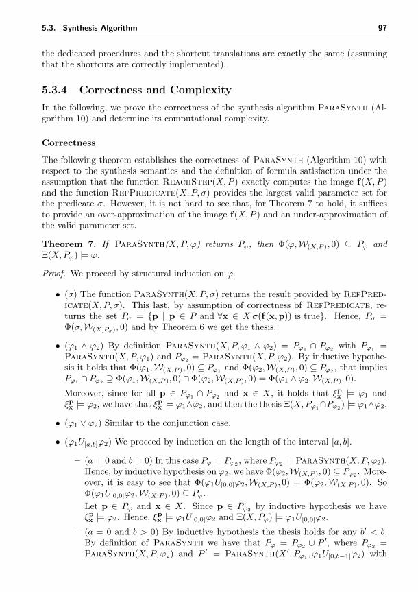
5.3. Synthesis Algorithm 97
the dedicated procedures and the shortcut translations are exactly the same (assumingthat the shortcuts are correctly implemented).
5.3.4 Correctness and Complexity
In the following, we prove the correctness of the synthesis algorithm ParaSynth (Al-gorithm 10) and determine its computational complexity.
Correctness
The following theorem establishes the correctness of ParaSynth (Algorithm 10) withrespect to the synthesis semantics and the definition of formula satisfaction under theassumption that the function ReachStep(X,P ) exactly computes the image f(X,P )and the function RefPredicate(X,P, σ) provides the largest valid parameter set forthe predicate σ. However, it is not hard to see that, for Theorem 7 to hold, it sufficesto provide an over-approximation of the image f(X,P ) and an under-approximation ofthe valid parameter set.
Theorem 7. If ParaSynth(X,P, ϕ) returns Pϕ, then Φ(ϕ,W(X,P ), 0) ⊆ Pϕ andΞ(X,Pϕ) |= ϕ.
Proof. We proceed by structural induction on ϕ.
• (σ) The function ParaSynth(X,P, σ) returns the result provided by RefPred-icate(X,P, σ). This last, by assumption of correctness of RefPredicate, re-turns the set Pσ = p | p ∈ P and ∀x ∈ X σ(f(x,p)) is true. Hence, Pσ =Φ(σ,W(X,Pσ), 0) and by Theorem 6 we get the thesis.
• (ϕ1 ∧ ϕ2) By definition ParaSynth(X,P, ϕ1 ∧ ϕ2) = Pϕ1∩ Pϕ2
with Pϕ1=
ParaSynth(X,P, ϕ1) and Pϕ2= ParaSynth(X,P, ϕ2). By inductive hypothe-
sis it holds that Φ(ϕ1,W(X,P ), 0) ⊆ Pϕ1and Φ(ϕ2,W(X,P ), 0) ⊆ Pϕ2
, that impliesPϕ1 ∩ Pϕ2 ⊇ Φ(ϕ1,W(X,P ), 0) ∩ Φ(ϕ2,W(X,P ), 0) = Φ(ϕ1 ∧ ϕ2,W(X,P ), 0).
Moreover, since for all p ∈ Pϕ1∩ Pϕ2
and x ∈ X, it holds that ξpx |= ϕ1 andξpx |= ϕ2, we have that ξpx |= ϕ1∧ϕ2, and then the thesis Ξ(X,Pϕ1
∩Pϕ2) |= ϕ1∧ϕ2.
• (ϕ1 ∨ ϕ2) Similar to the conjunction case.
• (ϕ1U[a,b]ϕ2) We proceed by induction on the length of the interval [a, b].
– (a = 0 and b = 0) In this case Pϕ = Pϕ2, where Pϕ2
= ParaSynth(X,P, ϕ2).Hence, by inductive hypothesis on ϕ2, we have Φ(ϕ2,W(X,P ), 0) ⊆ Pϕ2
. More-over, it is easy to see that Φ(ϕ1U[0,0]ϕ2,W(X,P ), 0) = Φ(ϕ2,W(X,P ), 0). SoΦ(ϕ1U[0,0]ϕ2,W(X,P ), 0) ⊆ Pϕ.
Let p ∈ Pϕ and x ∈ X. Since p ∈ Pϕ2 by inductive hypothesis we haveξpx |= ϕ2. Hence, ξpx |= ϕ1U[0,0]ϕ2 and Ξ(X,Pϕ) |= ϕ1U[0,0]ϕ2.
– (a = 0 and b > 0) By inductive hypothesis the thesis holds for any b′ < b.By definition of ParaSynth we have that Pϕ = Pϕ2 ∪ P ′, where Pϕ2 =ParaSynth(X,P, ϕ2) and P ′ = ParaSynth(X ′, Pϕ1 , ϕ1U[0,b−1]ϕ2) with
98 5. Parameter Synthesis
Pϕ1 = ParaSynth(X,P, ϕ1) and X ′ = ReachStep(X,Pϕ1). By inductivehypothesis we have that both the following inclusions hold:
Φ(ϕ2,W(X,P ), 0) ⊆ Pϕ2
Φ(ϕ1U[0,b−1]ϕ2,W(X′,Pϕ1 ), 0) ⊆ P ′.
To show the inclusion of the thesis, we now show that if a parameter pbelongs to Φ(ϕ1U[0,b]ϕ2,W(X,P ), 0), then it belongs also to Pϕ2 ∪ P ′. Sincep ∈ Φ(ϕ1U[0,b]ϕ2,W(X,P ), 0), by definition of synthesis semantics, it musthold that either p ∈ Φ(ϕ2,W(X,P ), 0), or there exists t′ ∈ [0, b] such thatp ∈ Φ(ϕ2,W(X,P ), t
′) and for all t′′ ∈ [0, t′], p ∈ Φ(ϕ1,W(X,P ), t′′). In the
first case, since p ∈ Φ(ϕ2,W(X,P ), 0), by inductive hypothesis we have thatp ∈ Pϕ2
. In the second case, we have that:
p ∈t′′⋂t′=0
Φ(ϕ1,W(X,P ), t′) ∩ Φ(ϕ2,W(X,P ), t
′′)
p ∈ Φ(ϕ1,W(X,P ), 0) ∩t′′⋂t′=1
Φ(ϕ1,W(X,P ), t′) ∩ Φ(ϕ2,W(X,P ), t
′′)
p ∈ Φ(ϕ1,W(X,P ), 0) ∩ Φ(ϕ1U[1,b]ϕ2,W(X,P ), 1)
p ∈ Φ(ϕ1,W(X,P ), 0) ∩ Φ(ϕ1U[0,b−1]ϕ2,W(f(X,P ),P ), 0)
Since X ′ = f(X,Pϕ1) ⊆ f(X,P ), it holds the inclusion:
Φ(ϕ1U[0,b−1]ϕ2,W(f(X,P ),P ), 0) ⊆ Φ(ϕ1U[0,b−1]ϕ2,W(X′,Pϕ1 ), 0) ⊆ P ′
from which, by inductive hypothesis, we deduce that p ∈ P ′.Let p ∈ Pϕ and x ∈ X. If p ∈ Pϕ2
, then we immediately get the thesis byinductive hypothesis. If p ∈ P ′, then p ∈ Pϕ1
and ξpx |= ϕ1. Hence, since P ′
is returned by ParaSynth(X ′, Pϕ1 , ϕ1U[0,b−1]ϕ2), by inductive hypothesiswe have that ξp
ξpx (1)|= ϕ1U[0,b−1]ϕ2. Hence, ξpx |= ϕ1U[0,b]ϕ2.
– (a > 0 and b > 0) Identical to the second part of the previous case.
Computational Complexity
Let us now determine the computational complexity of ParaSynth (Algorithm 10).As far as the computational complexity of our algorithm is concerned, let us refer toRefPredicate, ReachStep, ∪, and ∩ as symbolic operations. If we have a formulawithout until operators our procedure performs a number of symbolic operations thatis linear in the length of the formula. In the case of formulas with possibly nesteduntil operators, in the worst case, we could perform an exponential number of symbolicoperations with respect to the minimum between the length of the formula and its timehorizon.
5.4. The Polynomial Case 99
Let us consider the case of formulas using only predicates and U[0,1] operators. Letthe length of a formulas ϕ be defined as the maximum number of nested until operators.For a formula ϕ1U[0,1]ϕ2 having length m and horizon k our recursive procedure has arecursive complexity equation in term of symbolic operations of the form:
T (m, k) =
Θ(1) if m = 1 or k = 0
T (m2, k2) + T (m1, k1) + T (m, k − 1) + Θ(1) otherwise(5.22)
where mi and ki are the length and horizon of ϕi.
In the worst case we could have m2 = m− 2 and k2 = k − 1. In this case we obtainT (m, k) ≥ 2T (m − 2, k − 1) + Θ(1), which tells us that in the worst case T (m, k) =Ω(2min(m,k)) (number of symbolic operations). If we were interested in monitoring aformula over a finite set of traces, we could have reduced such complexity to a polynomialone (see, e.g., [143, 71]). As we already pointed out, since we are interested in refiningsets of parameters and to avoid rough approximations we do not use a precomputed setof traces, we do not see an easy way to reduce this complexity. However, it is importantto notice that the worst case complexity occurs only in very pathological cases, whichare not typical in real case studies.
5.4 The Polynomial Case
In the previous section we presented ParaSynth (Algorithm 10), an abstract algorithmthat synthesizes a parameter set under which the behaviors of a dynamical system satisfya given specification. A concrete application of ParaSynth depends on the ability ofrepresenting parameter sets and implementing the function ReachStep for computingthe system evolution, and the function RefPredicate for refining the parameter set.
We now propose a concretization of the algorithm for polynomial discrete-time dy-namical systems with polytopic parameter sets. However, notice that the abstract algo-rithm exposed in Section 5.3 can be used for more general systems as long as an imple-mentation of the required procedures are provided. An example might be continuous-time piecewise-linear dynamical systems, for which reachability techniques and toolshave been developed [6, 87].
From now on, we work with polynomial discrete-time dynamical systems of the formD = (X ,P, f), where X = Rn, P = Rm, and f : Rn×Rm → Rn is a polynomial. We alsoassume that the threated sets of parameters P ⊂ P are polytopes (see Section 4.1.1).For this class of dynamical systems and set representation we will show how to:
1. Manipulate parameter sets, namely, computing their intersections and symboli-cally representing their unions;
2. Implement the RechStep procedure, that over-approximates the single step evo-lution of the dynamical system;
3. Implement the RefPredicate procedure, that refines a parameter set so that theevolution of the system satisfies a given predicate within a single step.
100 5. Parameter Synthesis
5.4.1 Parameter Set Representation and Manipulation
The first implementation aspect we consider is the representation and manipulation ofsets of parameters. A polytope (see Section 4.1.1) is the simplest form that we use torepresent a parameter set. With the notation P = Ap ≤ b we mean that the parameterset P corresponds to the solution of the linear system Ap ≤ b. More complex parametersets can be obtained by the intersection and the union of several basic convex polytopes.
Let P1 = A1p ≤ b1 and P2 = A2p ≤ b2 be two convex polytopes. It is notdifficult to see that the intersection P1 ∩ P2 is the convex polytope that corresponds toP1 ∩ P2 = Ap ≤ b, where:
A =
(A1
A2
)and b =
(b1b2
). (5.23)
Less trivial is the union of two polytopes that might lead to a nonconvex set andconsequently the representation through a linear system may not be possible. For thisreason we symbolically represent the union of two polytopes P1 and P2 by simply keepingthe list of the corresponding linear systems. Formally, with a slight abuse of notation,P1 ∪ P2 is represented as P1 ∪ P2 = A1p ≤ b1, A2p ≤ b2.
It is now important to note that, thanks to the distributivity property, every param-eter set can be represented as the union of intersections. If a parameter set P is in theform:
P =
n⋃i=1
mi⋂j=1
Pi,j = (P1,1 ∩ . . . ∩ P1,m1) ∪ . . . ∪ (Pn,1 ∩ . . . ∩ Pn,mn) (5.24)
then it is said to be in union normal form. This form is suitable for our set representationsince the intersections of sets can be collapsed in a unique linear system while the unionscan be stored in single list.
Example 27. Let Pi = Aip ≤ bi for i = 1, . . . , 4 be parameter sets and P = P1 ∩ (P2 ∩(P3 ∪ P4)) whose union normal form is:
P1∩(P2∩(P3∪P4)
)= P1∩
((P2∩P3)∪
(P2∩P4)
)= (P1∩P2∩P3)∪(P1∩P2∩P4). (5.25)
Thus P = A′p ≤ b′, A′′p ≤ b′′ where:
A′ =
A1
A2
A3
;
b1b2b3
= b′ A′′ =
A1
A2
A4
;
b1b2b4
= b′′. (5.26)
5.4.2 Single Step Evolution
The second important element of an implementation of ParaSynth is the realization ofthe procedure ReachStep able to compute the single reachability step of the threateddynamical system.
Chapter 4 has been entirely dedicated to the realization of the set image algorithmReachStep. We have defined several techniques that depend on the representation of
5.4. The Polynomial Case 101
the reachable set. In particular, given a parametric polynomial f : Rn × Rm → Rn anda polytope P ⊂ Rm, we have seen how to over-approximate the set f(X,P ) with:
• X ⊂ Rn begin a box (see Section 4.3);
• X ⊂ Rn begin a parallelotope (see Section 4.4);
• X ⊂ Rn begin a symbolic polytope represented by a parallelotope bundle, i.e.,a collection of parallelotopes whose intersection generates a polytope (see Sec-tion 4.5).
We briefly recall that all the developed methods for determining an over-approximationset X ′ ⊇ f(X,P ) share similar key steps:
1. Define a transformation v(x) : Rn → Rn that maps the unit box to the set X;
2. Consider the composition f(v(x),p) and exploit Bernstein coefficients and theirproperties to bound the directions of X ′ over f(X,P ) (see Section 4.2);
3. Use the obtained bounds to construct a set X ′ ⊇ f(X,P ) that over-approximatesthe image of f(X,P ).
For the detailed descriptions of the mentioned methods, the reader can refer to Chap-ter 4.
5.4.3 Basic Refinement
Finally, we focus on the third and last basic element of ParaSynth, that is the im-plementation of the function RefPredicate that refines a parameter set so that thegiven dynamical system satisfies within a single step a given predicate.
We assume that the considered predicates σ = p(x) ≤ 0 are linear in x and thatall the coefficients ai(p) of the system dynamics f(x,p) are linear in the parameters p.These assumptions will allow us to recast the refinement problem in terms of a linearprogram.
Let D = (X ,P, f) be a discrete-time dynamical system and X ⊆ X be a set. Thetechnique we are going to expose can be applied in both the cases when X is a box ora parallelotope. Let v(x) : Rn → Rn be the map that transforms the unit box [0, 1]n
to the set X. In the case where X is a box, v(x) can be obtained with the functionmapUnitBoxTo (see Section 4.3). Otherwise, in the case where X is a parallelotope,v(x) corresponds to the generator function γU (q,β,x) obtainable with the functioncon2gen (see Section 4.4).
To check whether the system satisfies the predicate σ = p(x) ≤ 0 we consider thefunction g(x,p) = p(f(v(x),p)) and its Bernstein coefficients Bg = bi(p) | i ∈ Ig.Since the maximum Bernstein coefficients is an upper bound of the maximum of g(x,p),if we ensure that all the coefficients are smaller-equal than zero, then we are sure thatg(x,p) is smaller-equal than zero too, that corresponds saying that f(v(x),p) satisfiesthe predicate σ.
Formally, the following is a sufficient condition for the system to satisfy the predicateσ after one discrete step starting from the set X with parameter set P :
∀bi(p) ∈ Bg∀p ∈ P,bi(p) ≤ 0. (5.27)
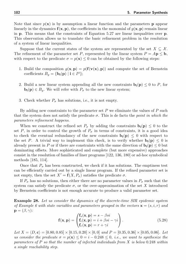
102 5. Parameter Synthesis
Note that since p(x) is by assumption a linear function and the parameters p appearlinearly in the dynamics f(x,p), the coefficients in the monomial of g(x,p) remain linearin p. This means that the constraints of Equation 5.27 are linear inequalities over p.This observation allows us to translate the basic refinement problem in the resolutionof a system of linear inequalities.
Suppose that the current states of the system are represented by the set X ⊆ X .The refinement of the parameter set P , represented by the linear system P = Ap ≤ b,with respect to the predicate σ = p(x) ≤ 0 can be obtained by the following steps:
1. Build the composition g(x,p) = p(f(v(x),p)) and compute the set of Bernsteincoefficients Bg = bi(p) | i ∈ Ig;
2. Build a new linear system appending all the new constraints bi(p) ≤ 0 to P , forbi(p) ∈ Bg. We will refer with Pσ to the new linear system;
3. Check whether Pσ has solutions, i.e., it is not empty.
By adding new constraints to the parameter set P we eliminate the values of P suchthat the system does not satisfy the predicate σ. This is de facto the point in which theparameters refinement happens.
When we construct the refined set Pσ by adding the constraints bi(p) ≤ 0 to theset P , in order to control the growth of Pσ in terms of constraints, it is a good ideato check the eventual redundancy of the new constraints bi(p) ≤ 0 with respect tothe set P . A trivial way to implement this check, is to verify whether bi(p) ≤ 0 isalready present in P or if there are constraints with the same direction of bi(p) ≤ 0 butdominating offsets. More sophisticated and complete (but more expensive) approachesconsist in the resolution of families of liner programs [122, 136, 180] or ad-hoc symbolicalmethods [185, 114].
Once that Pσ has been constructed, we check if it has solutions. The emptiness testcan be efficiently carried out by a single linear program. If the refined parameter set isnot empty, then the set X ′ = f(X,Pσ) satisfies the predicate σ.
If Pσ has no solutions, then either there are no parameter values in Pσ such that thesystem can satisfy the predicate σ, or the over-approximation of the set X introducedby Bernstein coefficients is not enough accurate to produce a valid parameter set.
Example 28. Let us consider the dynamics of the discrete-time SIR epidemic systemof Example 6 with state variables and parameters grouped in the vectors x = (s, i, r) andp = (β, γ):
f(x,p) =
fs(x,p) = s− βsifi(x,p) = i+ βsi− γifr(x,p) = r + γi
. (5.28)
Let X = 〈D, c〉 = [0.80, 0.85]× [0.15, 0.20]× [0, 0] and P = [0.35, 0.36]× [0.05, 0.06]. Letus consider the predicate σ = p(x) ≤ 0 = i − 0.248 ≤ 0, i.e., we want to synthesize theparameters of P so that the number of infected individuals from X is below 0.248 withina single reachability step.
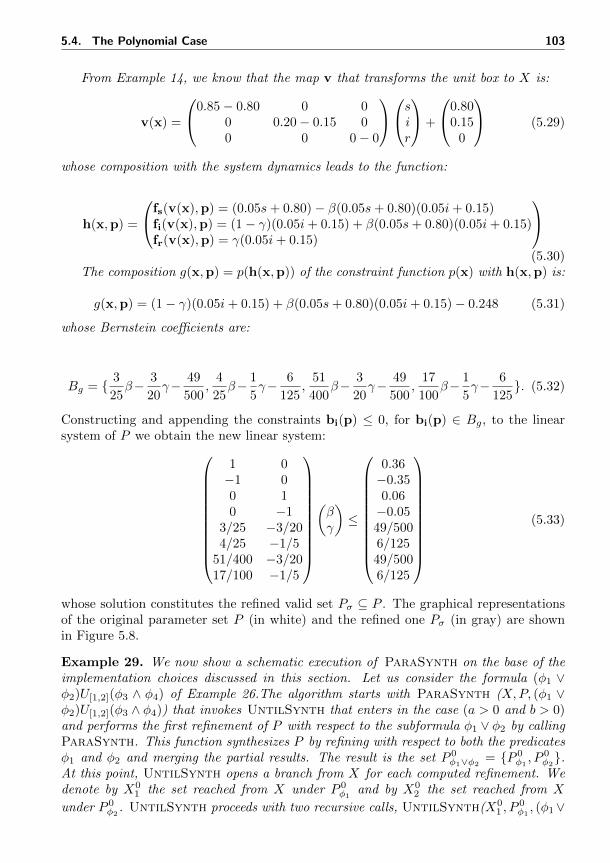
5.4. The Polynomial Case 103
From Example 14, we know that the map v that transforms the unit box to X is:
v(x) =
0.85− 0.80 0 00 0.20− 0.15 00 0 0− 0
sir
+
0.800.15
0
(5.29)
whose composition with the system dynamics leads to the function:
h(x,p) =
fs(v(x),p) = (0.05s+ 0.80)− β(0.05s+ 0.80)(0.05i+ 0.15)fi(v(x),p) = (1− γ)(0.05i+ 0.15) + β(0.05s+ 0.80)(0.05i+ 0.15)fr(v(x),p) = γ(0.05i+ 0.15)
(5.30)
The composition g(x,p) = p(h(x,p)) of the constraint function p(x) with h(x,p) is:
g(x,p) = (1− γ)(0.05i+ 0.15) + β(0.05s+ 0.80)(0.05i+ 0.15)− 0.248 (5.31)
whose Bernstein coefficients are:
Bg = 3
25β− 3
20γ− 49
500,
4
25β− 1
5γ− 6
125,
51
400β− 3
20γ− 49
500,
17
100β− 1
5γ− 6
125. (5.32)
Constructing and appending the constraints bi(p) ≤ 0, for bi(p) ∈ Bg, to the linearsystem of P we obtain the new linear system:
1 0−1 00 10 −1
3/25 −3/204/25 −1/5
51/400 −3/2017/100 −1/5
(βγ
)≤
0.36−0.350.06−0.0549/5006/12549/5006/125
(5.33)
whose solution constitutes the refined valid set Pσ ⊆ P . The graphical representationsof the original parameter set P (in white) and the refined one Pσ (in gray) are shownin Figure 5.8.
Example 29. We now show a schematic execution of ParaSynth on the base of theimplementation choices discussed in this section. Let us consider the formula (φ1 ∨φ2)U[1,2](φ3 ∧ φ4) of Example 26.The algorithm starts with ParaSynth (X,P, (φ1 ∨φ2)U[1,2](φ3 ∧ φ4)) that invokes UntilSynth that enters in the case (a > 0 and b > 0)and performs the first refinement of P with respect to the subformula φ1 ∨ φ2 by callingParaSynth. This function synthesizes P by refining with respect to both the predicatesφ1 and φ2 and merging the partial results. The result is the set P 0
φ1∨φ2= P 0
φ1, P 0
φ2.
At this point, UntilSynth opens a branch from X for each computed refinement. Wedenote by X0
1 the set reached from X under P 0φ1
and by X02 the set reached from X
under P 0φ2
. UntilSynth proceeds with two recursive calls, UntilSynth(X01 , P
0φ1, (φ1∨
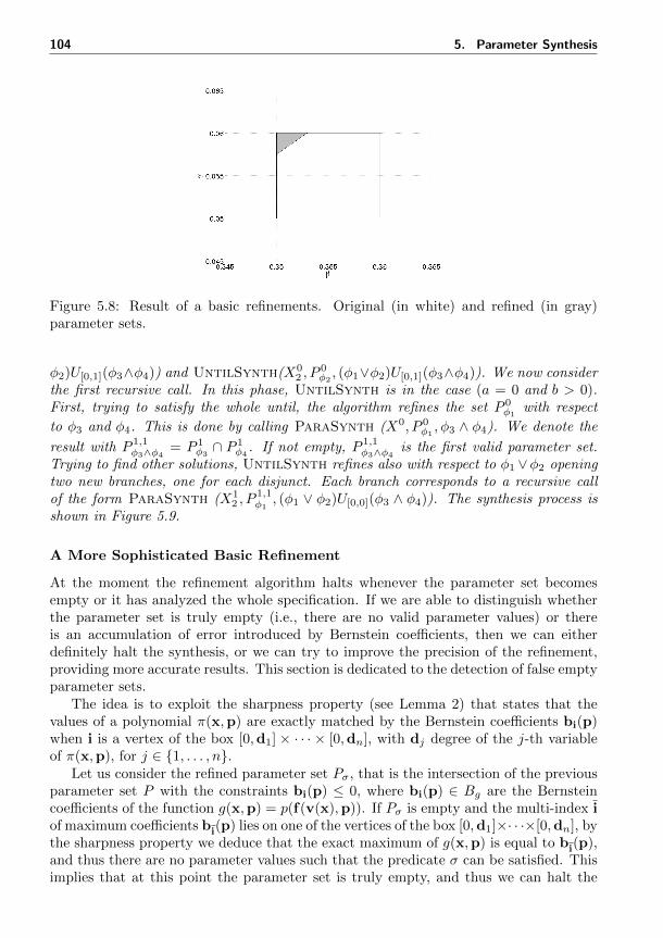
104 5. Parameter Synthesis
Figure 5.8: Result of a basic refinements. Original (in white) and refined (in gray)parameter sets.
φ2)U[0,1](φ3∧φ4)) and UntilSynth(X02 , P
0φ2, (φ1∨φ2)U[0,1](φ3∧φ4)). We now consider
the first recursive call. In this phase, UntilSynth is in the case (a = 0 and b > 0).First, trying to satisfy the whole until, the algorithm refines the set P 0
φ1with respect
to φ3 and φ4. This is done by calling ParaSynth (X0, P 0φ1, φ3 ∧ φ4). We denote the
result with P 1,1φ3∧φ4
= P 1φ3∩ P 1
φ4. If not empty, P 1,1
φ3∧φ4is the first valid parameter set.
Trying to find other solutions, UntilSynth refines also with respect to φ1 ∨φ2 openingtwo new branches, one for each disjunct. Each branch corresponds to a recursive callof the form ParaSynth (X1
2 , P1,1φ1, (φ1 ∨ φ2)U[0,0](φ3 ∧ φ4)). The synthesis process is
shown in Figure 5.9.
A More Sophisticated Basic Refinement
At the moment the refinement algorithm halts whenever the parameter set becomesempty or it has analyzed the whole specification. If we are able to distinguish whetherthe parameter set is truly empty (i.e., there are no valid parameter values) or thereis an accumulation of error introduced by Bernstein coefficients, then we can eitherdefinitely halt the synthesis, or we can try to improve the precision of the refinement,providing more accurate results. This section is dedicated to the detection of false emptyparameter sets.
The idea is to exploit the sharpness property (see Lemma 2) that states that thevalues of a polynomial π(x,p) are exactly matched by the Bernstein coefficients bi(p)when i is a vertex of the box [0,d1] × · · · × [0,dn], with dj degree of the j-th variableof π(x,p), for j ∈ 1, . . . , n.
Let us consider the refined parameter set Pσ, that is the intersection of the previousparameter set P with the constraints bi(p) ≤ 0, where bi(p) ∈ Bg are the Bernsteincoefficients of the function g(x,p) = p(f(v(x),p)). If Pσ is empty and the multi-index iof maximum coefficients bi(p) lies on one of the vertices of the box [0,d1]×· · ·×[0,dn], bythe sharpness property we deduce that the exact maximum of g(x,p) is equal to bi(p),and thus there are no parameter values such that the predicate σ can be satisfied. Thisimplies that at this point the parameter set is truly empty, and thus we can halt the
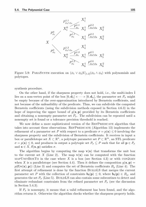
5.4. The Polynomial Case 105
X
X01
X02
X11
X12
X13
X14
X15
X16
X22
X23
X25
X26
P 0φ1
P 0φ2
P 1,1φ3∧φ4
P 1,1φ1
P 1,1φ2
P 1,2φ3∧φ4
P 1,2φ1
P 1,2φ2
P 2,2φ3∧φ4
P 2,3φ3∧φ4
P 2,5φ3∧φ4
P 2,6φ3∧φ4
Figure 5.9: ParaSynth execution on (φ1 ∨ φ2)U[1,2](φ3 ∧ φ4) with polynomials andpolytopes.
synthesis procedure.
On the other hand, if the sharpness property does not hold, i.e., the multi-index ilies on a non-vertex point of the box [0,d1]× · · · × [0,dn], the parameter set Pσ mightbe empty because of the over-approximation introduced by Bernstein coefficients, andnot because of the unfeasibility of the predicate. Thus, we can subdivide the computedBernstein coefficients (using the subdivision methods exposed in Section 4.6.3) in thehope of improving the upper bound of g(x,p) provided by its Bernstein coefficientsand obtaining a nonempty parameter set Pσ. The subdivision can be repeated until anonempty set is found or a tolerance precision threshold is reached.
We now define a more sophisticated version of the RefPredicate algorithm thattakes into account these observations. RefPredicate (Algorithm 13) implements therefinement of a parameter set P with respect to a predicate σ = p(x) ≤ 0 involving thesharpness property and the subdivision of Bernstein coefficients. It receives in input abox or parallelotope set X ⊂ Rn, a polytopic parameter set P ⊂ Rm, an STL predicateσ = p(x) ≤ 0, and produces in output a polytopic set Pσ ⊆ P such that for all p ∈ Pσand x ∈ X, f(x,p) satisfies σ.
The algorithm begins by computing the map v(x) that transforms the unit boxto the current set X (Line 2). The map v(x) can be computed with the functionmapUnitBoxTo in the case where X is a box (see Section 4.3) or with con2genwhen X is a parallelotope (see Section 4.4). Then it defines the composition g(x,p) =p(f(v(x),p)) (Line 3) and computes the set of Bernstein coefficients Bg (Line 4). Thefirst attempt of refinement is done by the function BuildLS that merges the currentparameter set P with the collection of constraints bi(p) ≤ 0, where bi(p) ∈ Bg, andgenerates the set Pσ (Line 5). BuildLS can also contain some subroutines to detect andeliminate redundant constraints from the refined parameter set Pσ (see the discussionin Section 5.4.3).
If Pσ is nonempty, it means that a valid refinement has been found, and the algo-rithm returns it. Otherwise the algorithm checks whether the sharpness property holds.
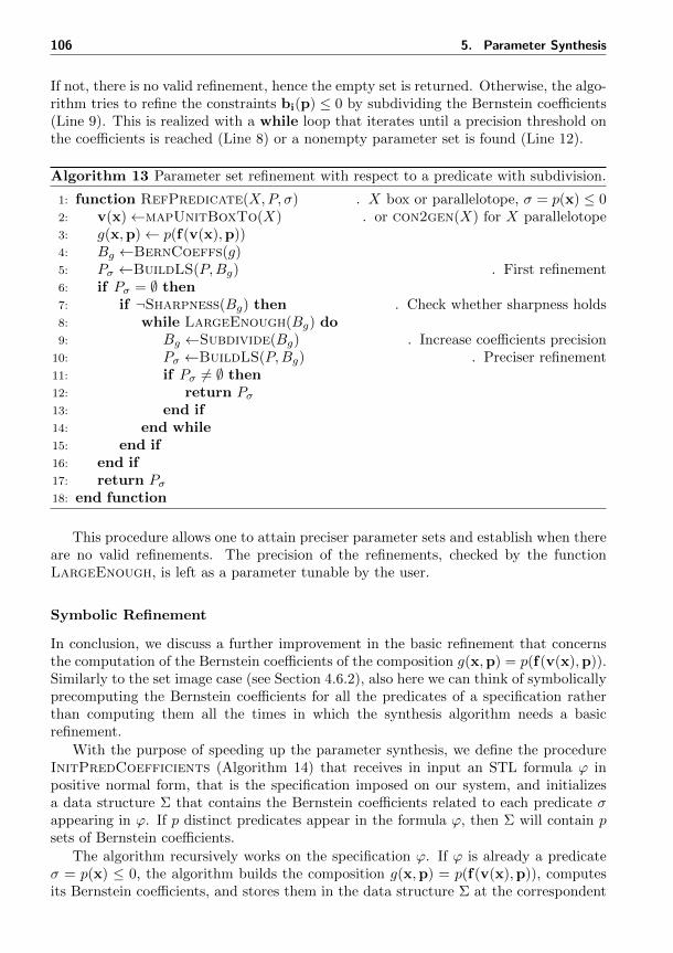
106 5. Parameter Synthesis
If not, there is no valid refinement, hence the empty set is returned. Otherwise, the algo-rithm tries to refine the constraints bi(p) ≤ 0 by subdividing the Bernstein coefficients(Line 9). This is realized with a while loop that iterates until a precision threshold onthe coefficients is reached (Line 8) or a nonempty parameter set is found (Line 12).
Algorithm 13 Parameter set refinement with respect to a predicate with subdivision.
1: function RefPredicate(X,P, σ) . X box or parallelotope, σ = p(x) ≤ 02: v(x)←mapUnitBoxTo(X) . or con2gen(X) for X parallelotope3: g(x,p)← p(f(v(x),p))4: Bg ←BernCoeffs(g)5: Pσ ←BuildLS(P,Bg) . First refinement6: if Pσ = ∅ then7: if ¬Sharpness(Bg) then . Check whether sharpness holds8: while LargeEnough(Bg) do9: Bg ←Subdivide(Bg) . Increase coefficients precision
10: Pσ ←BuildLS(P,Bg) . Preciser refinement11: if Pσ 6= ∅ then12: return Pσ13: end if14: end while15: end if16: end if17: return Pσ18: end function
This procedure allows one to attain preciser parameter sets and establish when thereare no valid refinements. The precision of the refinements, checked by the functionLargeEnough, is left as a parameter tunable by the user.
Symbolic Refinement
In conclusion, we discuss a further improvement in the basic refinement that concernsthe computation of the Bernstein coefficients of the composition g(x,p) = p(f(v(x),p)).Similarly to the set image case (see Section 4.6.2), also here we can think of symbolicallyprecomputing the Bernstein coefficients for all the predicates of a specification ratherthan computing them all the times in which the synthesis algorithm needs a basicrefinement.
With the purpose of speeding up the parameter synthesis, we define the procedureInitPredCoefficients (Algorithm 14) that receives in input an STL formula ϕ inpositive normal form, that is the specification imposed on our system, and initializesa data structure Σ that contains the Bernstein coefficients related to each predicate σappearing in ϕ. If p distinct predicates appear in the formula ϕ, then Σ will contain psets of Bernstein coefficients.
The algorithm recursively works on the specification ϕ. If ϕ is already a predicateσ = p(x) ≤ 0, the algorithm builds the composition g(x,p) = p(f(v(x),p)), computesits Bernstein coefficients, and stores them in the data structure Σ at the correspondent
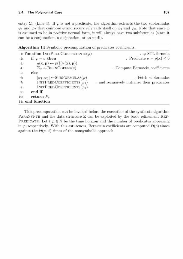
5.4. The Polynomial Case 107
entry Σσ (Line 4). If ϕ is not a predicate, the algorithm extracts the two subformulasϕ1 and ϕ2 that compose ϕ and recursively calls itself on ϕ1 and ϕ2. Note that since ϕis assumed to be in positive normal form, it will always have two subformulas (since itcan be a conjunction, a disjunction, or an until).
Algorithm 14 Symbolic precomputation of predicates coefficients.
1: function InitPredCoefficients(ϕ) . ϕ STL formula2: if ϕ = σ then . Predicate σ = p(x) ≤ 03: g(x,p)← p(f(v(x),p))4: Σσ ←BernCoeffs(g) . Compute Bernstein coefficients5: else6: [ϕ1, ϕ2]←SubFormulas(ϕ) . Fetch subformulas7: InitPredCoefficients(ϕ1) . and recursively initialize their predicates8: InitPredCoefficients(ϕ2)9: end if
10: return Pσ11: end function
This precomputation can be invoked before the execution of the synthesis algorithmParaSynth and the data structure Σ can be exploited by the basic refinement Ref-Predicate. Let t, p ∈ N be the time horizon and the number of predicates appearingin ϕ, respectively. With this astuteness, Bernstein coefficients are computed Θ(p) timesagainst the Θ(p · t) times of the nonsymbolic approach.

6Tool and Experimental Results
This chapter is devoted to the description and evaluation of the tool Sapo that imple-ments the reachability and parameter synthesis techniques previously described. Thedeveloped techniques and tool are assessed on some polynomial dynamical systems forboth reachability analysis and parameter synthesis. We will analyze artificial, biological,and mechanical models.
The chapter is organized in two main sections. In the first (Section 6.1), we willdescribe our tool, focusing on its structure, highlighting its main features, and ourimplementation choices. In the second (Section 6.2), we will exercise and evaluate Sapoon some polynomial parametric discrete-time dynamical systems.
6.1 Architecture
We begin with the description of the tool Sapo that gathers the implementations ofthe reachability and parameter synthesis techniques previously described. The overallarchitecture of Sapo is summarized in Figure 6.1.
The main module of the tool is Sapo (Section 6.1.1), that handles the computation ofreachable sets and the synthesis of parameters. Another important module is the Base
Converter (Section 6.1.4) that allows us to compute the Bernstein coefficients of a givenpolynomial. The Bundle and Parallelotope modules (Sections 6.1.5 and 6.1.6) areused to represent sets of states of dynamical systems, while Linear System and Linear
System Set (Sections 6.1.8 and 6.1.9) are used for representing sets of parameters. WithSTL and Model (Sections 6.1.2 and 6.1.3) the user can formalize a specification andinstantiate a polynomial dynamical system. Finally, Vars Generator (Section 6.1.7) isa utility module that can be used to automatize the declaration of the variables necessaryto instantiate a parallelotope.
Our tool is entirely implemented in C++. It relies on the libraries GiNaC (GiNaCis not a CAS) [19] and GLPK (GNU Linear Programming Kit).1 GiNaC is used for thesymbolic representation of polynomials. In the following, by “symbolic expression” we
1http://www.gnu.org/software/glpk/glpk.html
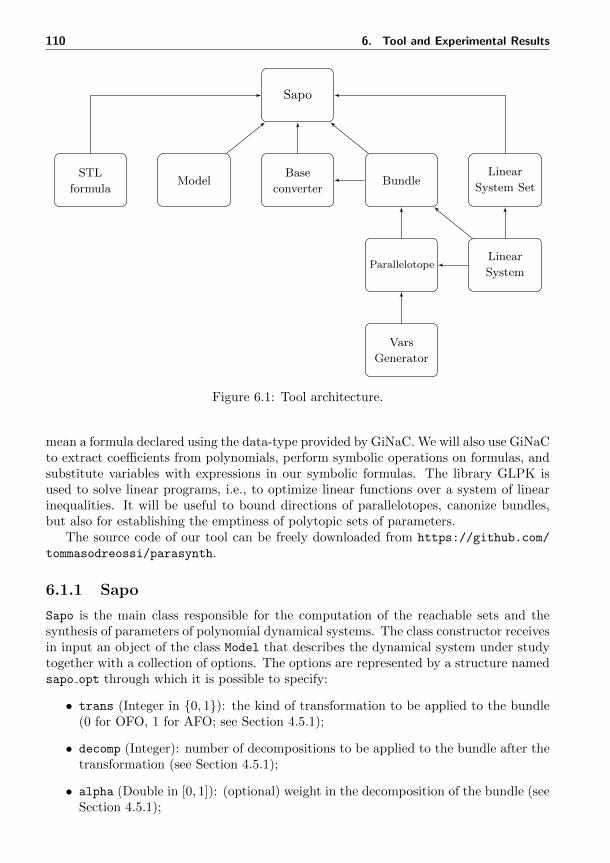
110 6. Tool and Experimental Results
Sapo
Base
converterBundle
Linear
System SetModel
STL
formula
ParallelotopeLinear
System
Vars
Generator
Figure 6.1: Tool architecture.
mean a formula declared using the data-type provided by GiNaC. We will also use GiNaCto extract coefficients from polynomials, perform symbolic operations on formulas, andsubstitute variables with expressions in our symbolic formulas. The library GLPK isused to solve linear programs, i.e., to optimize linear functions over a system of linearinequalities. It will be useful to bound directions of parallelotopes, canonize bundles,but also for establishing the emptiness of polytopic sets of parameters.
The source code of our tool can be freely downloaded from https://github.com/
tommasodreossi/parasynth.
6.1.1 Sapo
Sapo is the main class responsible for the computation of the reachable sets and thesynthesis of parameters of polynomial dynamical systems. The class constructor receivesin input an object of the class Model that describes the dynamical system under studytogether with a collection of options. The options are represented by a structure namedsapo opt through which it is possible to specify:
• trans (Integer in 0, 1): the kind of transformation to be applied to the bundle(0 for OFO, 1 for AFO; see Section 4.5.1);
• decomp (Integer): number of decompositions to be applied to the bundle after thetransformation (see Section 4.5.1);
• alpha (Double in [0, 1]): (optional) weight in the decomposition of the bundle (seeSection 4.5.1);
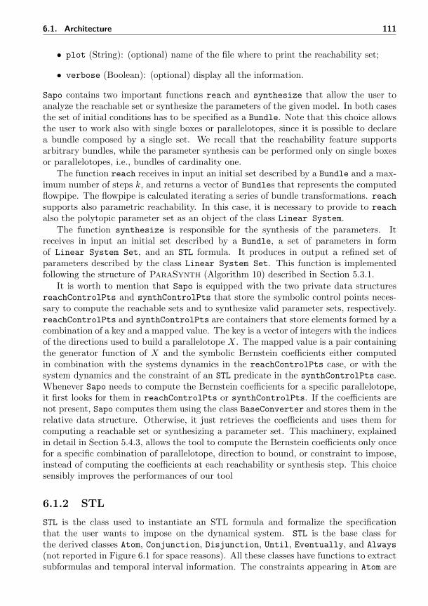
6.1. Architecture 111
• plot (String): (optional) name of the file where to print the reachability set;
• verbose (Boolean): (optional) display all the information.
Sapo contains two important functions reach and synthesize that allow the user toanalyze the reachable set or synthesize the parameters of the given model. In both casesthe set of initial conditions has to be specified as a Bundle. Note that this choice allowsthe user to work also with single boxes or parallelotopes, since it is possible to declarea bundle composed by a single set. We recall that the reachability feature supportsarbitrary bundles, while the parameter synthesis can be performed only on single boxesor parallelotopes, i.e., bundles of cardinality one.
The function reach receives in input an initial set described by a Bundle and a max-imum number of steps k, and returns a vector of Bundles that represents the computedflowpipe. The flowpipe is calculated iterating a series of bundle transformations. reachsupports also parametric reachability. In this case, it is necessary to provide to reach
also the polytopic parameter set as an object of the class Linear System.The function synthesize is responsible for the synthesis of the parameters. It
receives in input an initial set described by a Bundle, a set of parameters in formof Linear System Set, and an STL formula. It produces in output a refined set ofparameters described by the class Linear System Set. This function is implementedfollowing the structure of ParaSynth (Algorithm 10) described in Section 5.3.1.
It is worth to mention that Sapo is equipped with the two private data structuresreachControlPts and synthControlPts that store the symbolic control points neces-sary to compute the reachable sets and to synthesize valid parameter sets, respectively.reachControlPts and synthControlPts are containers that store elements formed by acombination of a key and a mapped value. The key is a vector of integers with the indicesof the directions used to build a parallelotope X. The mapped value is a pair containingthe generator function of X and the symbolic Bernstein coefficients either computedin combination with the systems dynamics in the reachControlPts case, or with thesystem dynamics and the constraint of an STL predicate in the synthControlPts case.Whenever Sapo needs to compute the Bernstein coefficients for a specific parallelotope,it first looks for them in reachControlPts or synthControlPts. If the coefficients arenot present, Sapo computes them using the class BaseConverter and stores them in therelative data structure. Otherwise, it just retrieves the coefficients and uses them forcomputing a reachable set or synthesizing a parameter set. This machinery, explainedin detail in Section 5.4.3, allows the tool to compute the Bernstein coefficients only oncefor a specific combination of parallelotope, direction to bound, or constraint to impose,instead of computing the coefficients at each reachability or synthesis step. This choicesensibly improves the performances of our tool
6.1.2 STL
STL is the class used to instantiate an STL formula and formalize the specificationthat the user wants to impose on the dynamical system. STL is the base class forthe derived classes Atom, Conjunction, Disjunction, Until, Eventually, and Always
(not reported in Figure 6.1 for space reasons). All these classes have functions to extractsubformulas and temporal interval information. The constraints appearing in Atom are
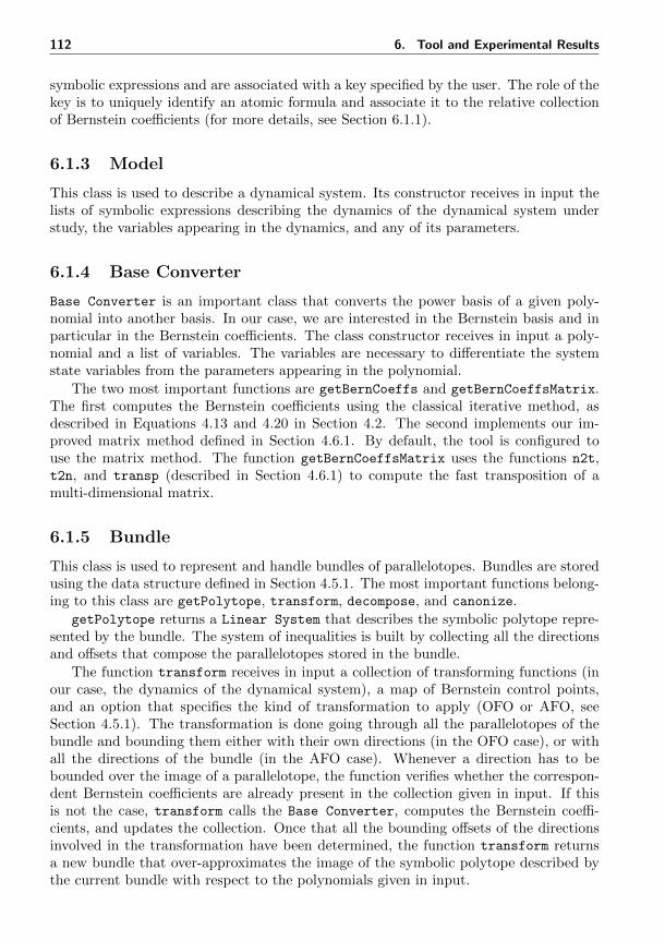
112 6. Tool and Experimental Results
symbolic expressions and are associated with a key specified by the user. The role of thekey is to uniquely identify an atomic formula and associate it to the relative collectionof Bernstein coefficients (for more details, see Section 6.1.1).
6.1.3 Model
This class is used to describe a dynamical system. Its constructor receives in input thelists of symbolic expressions describing the dynamics of the dynamical system understudy, the variables appearing in the dynamics, and any of its parameters.
6.1.4 Base Converter
Base Converter is an important class that converts the power basis of a given poly-nomial into another basis. In our case, we are interested in the Bernstein basis and inparticular in the Bernstein coefficients. The class constructor receives in input a poly-nomial and a list of variables. The variables are necessary to differentiate the systemstate variables from the parameters appearing in the polynomial.
The two most important functions are getBernCoeffs and getBernCoeffsMatrix.The first computes the Bernstein coefficients using the classical iterative method, asdescribed in Equations 4.13 and 4.20 in Section 4.2. The second implements our im-proved matrix method defined in Section 4.6.1. By default, the tool is configured touse the matrix method. The function getBernCoeffsMatrix uses the functions n2t,t2n, and transp (described in Section 4.6.1) to compute the fast transposition of amulti-dimensional matrix.
6.1.5 Bundle
This class is used to represent and handle bundles of parallelotopes. Bundles are storedusing the data structure defined in Section 4.5.1. The most important functions belong-ing to this class are getPolytope, transform, decompose, and canonize.
getPolytope returns a Linear System that describes the symbolic polytope repre-sented by the bundle. The system of inequalities is built by collecting all the directionsand offsets that compose the parallelotopes stored in the bundle.
The function transform receives in input a collection of transforming functions (inour case, the dynamics of the dynamical system), a map of Bernstein control points,and an option that specifies the kind of transformation to apply (OFO or AFO, seeSection 4.5.1). The transformation is done going through all the parallelotopes of thebundle and bounding them either with their own directions (in the OFO case), or withall the directions of the bundle (in the AFO case). Whenever a direction has to bebounded over the image of a parallelotope, the function verifies whether the correspon-dent Bernstein coefficients are already present in the collection given in input. If thisis not the case, transform calls the Base Converter, computes the Bernstein coeffi-cients, and updates the collection. Once that all the bounding offsets of the directionsinvolved in the transformation have been determined, the function transform returnsa new bundle that over-approximates the image of the symbolic polytope described bythe current bundle with respect to the polynomials given in input.
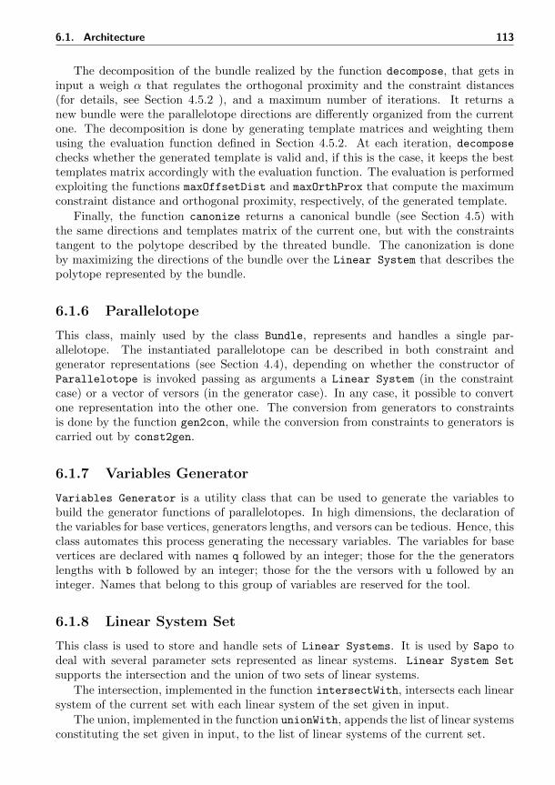
6.1. Architecture 113
The decomposition of the bundle realized by the function decompose, that gets ininput a weigh α that regulates the orthogonal proximity and the constraint distances(for details, see Section 4.5.2 ), and a maximum number of iterations. It returns anew bundle were the parallelotope directions are differently organized from the currentone. The decomposition is done by generating template matrices and weighting themusing the evaluation function defined in Section 4.5.2. At each iteration, decompose
checks whether the generated template is valid and, if this is the case, it keeps the besttemplates matrix accordingly with the evaluation function. The evaluation is performedexploiting the functions maxOffsetDist and maxOrthProx that compute the maximumconstraint distance and orthogonal proximity, respectively, of the generated template.
Finally, the function canonize returns a canonical bundle (see Section 4.5) withthe same directions and templates matrix of the current one, but with the constraintstangent to the polytope described by the threated bundle. The canonization is doneby maximizing the directions of the bundle over the Linear System that describes thepolytope represented by the bundle.
6.1.6 Parallelotope
This class, mainly used by the class Bundle, represents and handles a single par-allelotope. The instantiated parallelotope can be described in both constraint andgenerator representations (see Section 4.4), depending on whether the constructor ofParallelotope is invoked passing as arguments a Linear System (in the constraintcase) or a vector of versors (in the generator case). In any case, it possible to convertone representation into the other one. The conversion from generators to constraintsis done by the function gen2con, while the conversion from constraints to generators iscarried out by const2gen.
6.1.7 Variables Generator
Variables Generator is a utility class that can be used to generate the variables tobuild the generator functions of parallelotopes. In high dimensions, the declaration ofthe variables for base vertices, generators lengths, and versors can be tedious. Hence, thisclass automates this process generating the necessary variables. The variables for basevertices are declared with names q followed by an integer; those for the the generatorslengths with b followed by an integer; those for the the versors with u followed by aninteger. Names that belong to this group of variables are reserved for the tool.
6.1.8 Linear System Set
This class is used to store and handle sets of Linear Systems. It is used by Sapo todeal with several parameter sets represented as linear systems. Linear System Set
supports the intersection and the union of two sets of linear systems.
The intersection, implemented in the function intersectWith, intersects each linearsystem of the current set with each linear system of the set given in input.
The union, implemented in the function unionWith, appends the list of linear systemsconstituting the set given in input, to the list of linear systems of the current set.
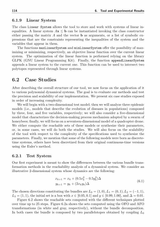
114 6. Tool and Experimental Results
6.1.9 Linear System
The class Linear System allows the tool to store and work with systems of linear in-equalities. A linear system Ax ≤ b can be instantiated invoking the class constructoreither passing the matrix A and the vector b as arguments, or a list of symbolic ex-pressions that are the constraints representing the inequalities of the system and thevariables that appear in them.
The functions maxLinearSystem and minLinearSystem offer the possibility of max-imizing or minimizing, respectively, an objective linear function over the current linearsystem. The optimization of the linear function is performed relying on the libraryGLPK (GNU Linear Programming Kit). Finally, the function appendLinearSystem
appends a linear system to the current one. This function can be used to intersect twopolytopes represented through linear systems.
6.2 Case Studies
After describing the overall structure of our tool, we now focus on the application of itto various polynomial dynamical systems. The goal is to evaluate our methods and testthe precision and scalability of our implementation. We present six case studies exposedin order of increasing complexity.
We will begin with a two-dimensional test model; then we will analyze three epidemicmodels (i.e., models that describe the evolution of diseases in populations) composedby three, four, and five variables, respectively; we will also consider a five-dimensionalmodel that characterizes the decision-making process mechanism adopted by a swarm ofhoneybees; finally, we will focus on a seventeen-dimensional model of a quadcopter drone.We either compute the reachable sets of these models or synthesize their parameters,or, in some cases, we will do both the studies. We will also focus on the scalabilityof the tool with respect to the complexity of the specifications used to synthesize theparameters. Finally, we mention that some of the following models were born as discrete-time systems, others have been discretized from their original continuous-time versionsusing the Euler’s method.
6.2.1 Test System
Our first experiment is meant to show the differences between the various bundle trans-formation methods in the reachability analysis of a dynamical system. We consider anillustrative 2-dimensional system whose dynamics are the following:
xk+1 = xk + (0.5x2k − 0.5y2k)∆
yk+1 = yk + (2xkyk)∆(6.1)
The chosen directions constituting the bundles are L0 = (1, 0), L1 = (0, 1), L2 = (−1, 1),L3 = (1, 1), the initial set is a box with x ∈ [0.05, 0.1] and y ∈ [0.99, 1.00], and ∆ = 0.01.
Figure 6.2 shows the reachable sets computed with the different techniques plottedover time up to 25 steps. Figure 6.2a shows the sets computed using the OFO and AFOtransformations (in white and gray, respectively), without the bundle decomposition.In both cases the bundle is composed by two parallelotopes obtained by coupling L0
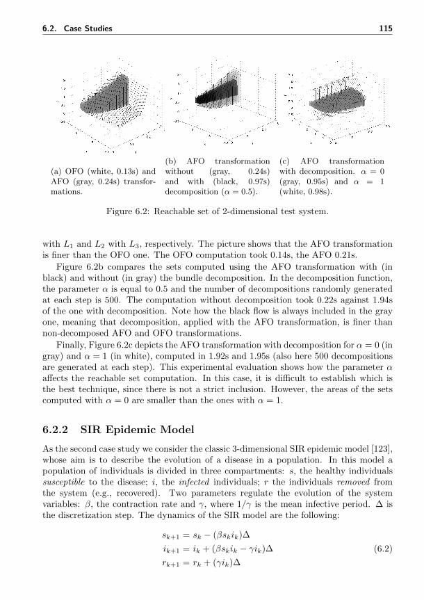
6.2. Case Studies 115
(a) OFO (white, 0.13s) andAFO (gray, 0.24s) transfor-mations.
(b) AFO transformationwithout (gray, 0.24s)and with (black, 0.97s)decomposition (α = 0.5).
(c) AFO transformationwith decomposition. α = 0(gray, 0.95s) and α = 1(white, 0.98s).
Figure 6.2: Reachable set of 2-dimensional test system.
with L1 and L2 with L3, respectively. The picture shows that the AFO transformationis finer than the OFO one. The OFO computation took 0.14s, the AFO 0.21s.
Figure 6.2b compares the sets computed using the AFO transformation with (inblack) and without (in gray) the bundle decomposition. In the decomposition function,the parameter α is equal to 0.5 and the number of decompositions randomly generatedat each step is 500. The computation without decomposition took 0.22s against 1.94sof the one with decomposition. Note how the black flow is always included in the grayone, meaning that decomposition, applied with the AFO transformation, is finer thannon-decomposed AFO and OFO transformations.
Finally, Figure 6.2c depicts the AFO transformation with decomposition for α = 0 (ingray) and α = 1 (in white), computed in 1.92s and 1.95s (also here 500 decompositionsare generated at each step). This experimental evaluation shows how the parameter αaffects the reachable set computation. In this case, it is difficult to establish which isthe best technique, since there is not a strict inclusion. However, the areas of the setscomputed with α = 0 are smaller than the ones with α = 1.
6.2.2 SIR Epidemic Model
As the second case study we consider the classic 3-dimensional SIR epidemic model [123],whose aim is to describe the evolution of a disease in a population. In this model apopulation of individuals is divided in three compartments: s, the healthy individualssusceptible to the disease; i, the infected individuals; r the individuals removed fromthe system (e.g., recovered). Two parameters regulate the evolution of the systemvariables: β, the contraction rate and γ, where 1/γ is the mean infective period. ∆ isthe discretization step. The dynamics of the SIR model are the following:
sk+1 = sk − (βskik)∆
ik+1 = ik + (βskik − γik)∆
rk+1 = rk + (γik)∆
(6.2)
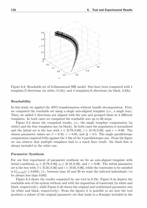
116 6. Tool and Experimental Results
Figure 6.3: Reachable set of 3-dimensional SIR model. Sets have been computed with 1template/3 directions (in white, 0.12s), and 4 templates/6 directions (in black, 2.83s).
Reachability
In this study we applied the AFO transformation without bundle decomposition. First,we computed the reachable set using a single axis-aligned template (i.e., a single box).Then, we added 5 directions not aligned with the axis and grouped them in 4 differenttemplates. In both cases we computed the reachable sets up to 60 steps.
Figure 6.3 shows the computed results, i.e., the single template computation (inwhite) and the four templates one (in black). In both cases the population is normalizedand the initial set is the box with s ∈ [0.79, 0.80], i ∈ [0.19, 0.20], and r = 0.00. Thechosen parameter values are β = 0.34, γ = 0.05, and ∆ = 0.5. The single parallelotopecomputation required 0.05s against the 1.04s of the 4 parallelotopes one. From the figurewe can observe that multiple templates lead to a much finer result: the black flow isalways included in the white one.
Parameter Synthesis
For our first experiment of parameter synthesis we fix an axis-aligned template withinitial conditions s0 ∈ [0.79, 0.80], i0 ∈ [0.19, 0.20], and r = 0.00. The initial parameterset is the box with β ∈ [0.35, 0.36] and γ ∈ [0.05, 0.06], while the constraint to be satisfiedis G[10,30](i ≤ 0.682), i.e., between time 10 and 30 we want the infected individuals i tobe always less than 0.682.
Figure 6.4 shows the results computed by our tool in 0.10s. Figure 6.4a depicts thereachable sets of the system without and with the imposition of constraint (in white andblack, respectively), while Figure 6.4b shows the original and synthesized parameter sets(in white and black, respectively). From the figures it is possible to see how the toolproduces a subset of the original parameter set that leads to a flowpipe included in the
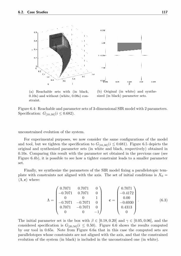
6.2. Case Studies 117
(a) Reachable sets with (in black,0.10s) and without (white, 0.08s) con-straint.
(b) Original (in white) and synthe-sized (in black) parameter sets.
Figure 6.4: Reachable and parameter sets of 3-dimensional SIR model with 2 parameters.Specification: G[10,30](i ≤ 0.682).
unconstrained evolution of the system.
For experimental purposes, we now consider the same configurations of the modeland tool, but we tighten the specification to G[10,30](i ≤ 0.681). Figure 6.5 depicts theoriginal and synthesized parameter sets (in white and black, respectively) obtained in0.10s. Comparing this result with the parameter set obtained in the previous case (seeFigure 6.4b), it is possible to see how a tighter constraint leads to a smaller parameterset.
Finally, we synthesize the parameters of the SIR model fixing a parallelotopic tem-plate with constraints not aligned with the axis. The set of initial conditions is X0 =〈Λ, c〉 where:
Λ =
0.7071 0.7071 0−0.7071 0.7071 0
0 0 1−0.7071 −0.7071 00.7071 −0.7071 0
0 0 −1
c =
0.7071−0.4172
0.00−0.69300.4313
0
. (6.3)
The initial parameter set is the box with β ∈ [0.18, 0.20] and γ ∈ [0.05, 0.06], and theconsidered specification is G[20,50](i ≤ 0.50). Figure 6.6 shows the results computedby our tool in 0.65s. Note from Figure 6.6a that in this case the computed sets areparallelotopes whose constraints are not aligned with the axis, and that the constrainedevolution of the system (in black) is included in the unconstrained one (in white).
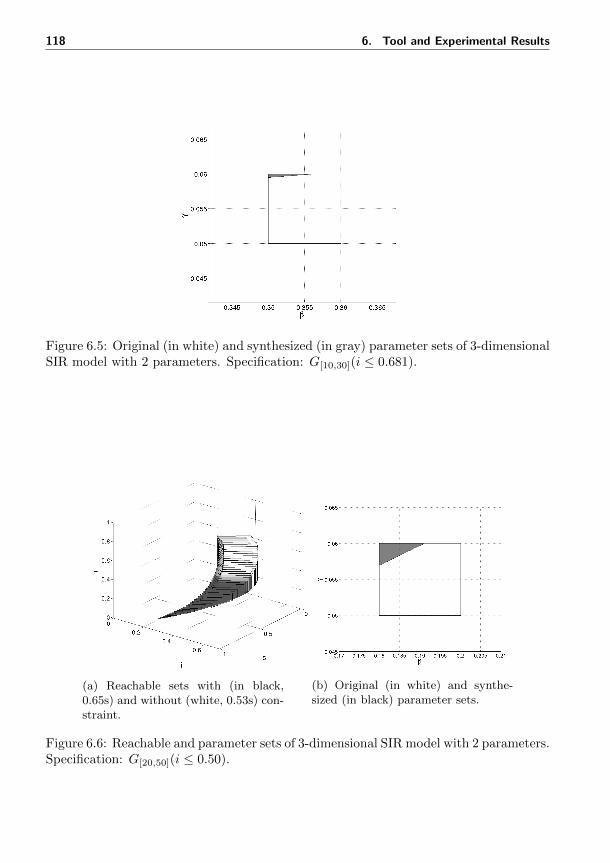
118 6. Tool and Experimental Results
Figure 6.5: Original (in white) and synthesized (in gray) parameter sets of 3-dimensionalSIR model with 2 parameters. Specification: G[10,30](i ≤ 0.681).
(a) Reachable sets with (in black,0.65s) and without (white, 0.53s) con-straint.
(b) Original (in white) and synthe-sized (in black) parameter sets.
Figure 6.6: Reachable and parameter sets of 3-dimensional SIR model with 2 parameters.Specification: G[20,50](i ≤ 0.50).
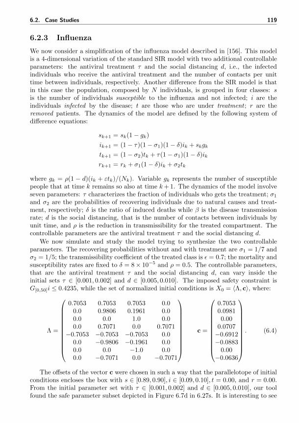
6.2. Case Studies 119
6.2.3 Influenza
We now consider a simplification of the influenza model described in [156]. This modelis a 4-dimensional variation of the standard SIR model with two additional controllableparameters: the antiviral treatment τ and the social distancing d, i.e., the infectedindividuals who receive the antiviral treatment and the number of contacts per unittime between individuals, respectively. Another difference from the SIR model is thatin this case the population, composed by N individuals, is grouped in four classes: sis the number of individuals susceptible to the influenza and not infected; i are theindividuals infected by the disease; t are those who are under treatment ; r are theremoved patients. The dynamics of the model are defined by the following system ofdifference equations:
sk+1 = sk(1− gk)
ik+1 = (1− τ)(1− σ1)(1− δ)ik + skgk
tk+1 = (1− σ2)tk + τ(1− σ1)(1− δ)ikrk+1 = rk + σ1(1− δ)ik + σ2tk
where gk = ρ(1 − d)(ik + εtk)/(Nk). Variable gk represents the number of susceptiblepeople that at time k remains so also at time k+ 1. The dynamics of the model involveseven parameters: τ characterizes the fraction of individuals who gets the treatment; σ1and σ2 are the probabilities of recovering individuals due to natural causes and treat-ment, respectively; δ is the ratio of induced deaths while β is the disease transmissionrate; d is the social distancing, that is the number of contacts between individuals byunit time, and ρ is the reduction in transmissibility for the treated compartment. Thecontrollable parameters are the antiviral treatment τ and the social distancing d.
We now simulate and study the model trying to synthesize the two controllableparameters. The recovering probabilities without and with treatment are σ1 = 1/7 andσ2 = 1/5; the transmissibility coefficient of the treated class is ε = 0.7; the mortality andsusceptibility rates are fixed to δ = 8× 10⁻⁵ and ρ = 0.5. The controllable parameters,that are the antiviral treatment τ and the social distancing d, can vary inside theinitial sets τ ∈ [0.001, 0.002] and d ∈ [0.005, 0.010]. The imposed safety constraint isG[0,50]i ≤ 0.4235, while the set of normalized initial conditions is X0 = 〈Λ, c〉, where:
Λ =
0.7053 0.7053 0.7053 0.00.0 0.9806 0.1961 0.00.0 0.0 1.0 0.00.0 0.7071 0.0 0.7071
−0.7053 −0.7053 −0.7053 0.00.0 −0.9806 −0.1961 0.00.0 0.0 −1.0 0.00.0 −0.7071 0.0 −0.7071
c =
0.70530.09810.00
0.0707−0.6912−0.0883
0.00−0.0636
. (6.4)
The offsets of the vector c were chosen in such a way that the parallelotope of initialconditions encloses the box with s ∈ [0.89, 0.90], i ∈ [0.09, 0.10], t = 0.00, and r = 0.00.From the initial parameter set with τ ∈ [0.001, 0.002] and d ∈ [0.005, 0.010], our toolfound the safe parameter subset depicted in Figure 6.7d in 6.27s. It is interesting to see
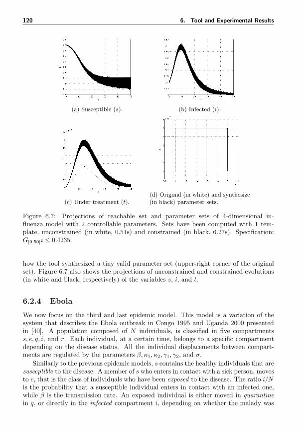
120 6. Tool and Experimental Results
(a) Susceptible (s). (b) Infected (i).
(c) Under treatment (t).(d) Original (in white) and synthesize(in black) parameter sets.
Figure 6.7: Projections of reachable set and parameter sets of 4-dimensional in-fluenza model with 2 controllable parameters. Sets have been computed with 1 tem-plate, unconstrained (in white, 0.51s) and constrained (in black, 6.27s). Specification:G[0,50]i ≤ 0.4235.
how the tool synthesized a tiny valid parameter set (upper-right corner of the originalset). Figure 6.7 also shows the projections of unconstrained and constrained evolutions(in white and black, respectively) of the variables s, i, and t.
6.2.4 Ebola
We now focus on the third and last epidemic model. This model is a variation of thesystem that describes the Ebola outbreak in Congo 1995 and Uganda 2000 presentedin [40]. A population composed of N individuals, is classified in five compartmentss, e, q, i, and r. Each individual, at a certain time, belongs to a specific compartmentdepending on the disease status. All the individual displacements between compart-ments are regulated by the parameters β, κ1, κ2, γ1, γ2, and σ.
Similarly to the previous epidemic models, s contains the healthy individuals that aresusceptible to the disease. A member of s who enters in contact with a sick person, movesto e, that is the class of individuals who have been exposed to the disease. The ratio i/Nis the probability that a susceptible individual enters in contact with an infected one,while β is the transmission rate. An exposed individual is either moved in quarantinein q, or directly in the infected compartment i, depending on whether the malady was
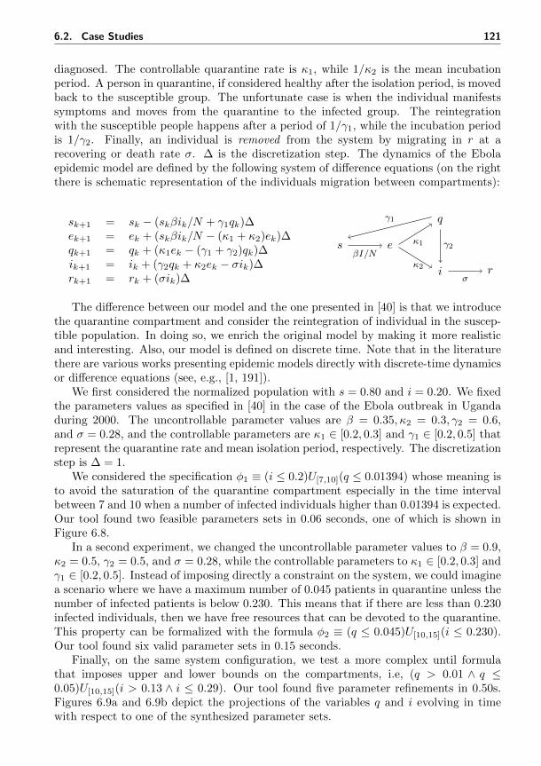
6.2. Case Studies 121
diagnosed. The controllable quarantine rate is κ1, while 1/κ2 is the mean incubationperiod. A person in quarantine, if considered healthy after the isolation period, is movedback to the susceptible group. The unfortunate case is when the individual manifestssymptoms and moves from the quarantine to the infected group. The reintegrationwith the susceptible people happens after a period of 1/γ1, while the incubation periodis 1/γ2. Finally, an individual is removed from the system by migrating in r at arecovering or death rate σ. ∆ is the discretization step. The dynamics of the Ebolaepidemic model are defined by the following system of difference equations (on the rightthere is schematic representation of the individuals migration between compartments):
sk+1 = sk − (skβik/N + γ1qk)∆ek+1 = ek + (skβik/N − (κ1 + κ2)ek)∆qk+1 = qk + (κ1ek − (γ1 + γ2)qk)∆ik+1 = ik + (γ2qk + κ2ek − σik)∆rk+1 = rk + (σik)∆
s e
q
i r
βI/N
κ1
κ2
γ1
γ2
σ
The difference between our model and the one presented in [40] is that we introducethe quarantine compartment and consider the reintegration of individual in the suscep-tible population. In doing so, we enrich the original model by making it more realisticand interesting. Also, our model is defined on discrete time. Note that in the literaturethere are various works presenting epidemic models directly with discrete-time dynamicsor difference equations (see, e.g., [1, 191]).
We first considered the normalized population with s = 0.80 and i = 0.20. We fixedthe parameters values as specified in [40] in the case of the Ebola outbreak in Ugandaduring 2000. The uncontrollable parameter values are β = 0.35, κ2 = 0.3, γ2 = 0.6,and σ = 0.28, and the controllable parameters are κ1 ∈ [0.2, 0.3] and γ1 ∈ [0.2, 0.5] thatrepresent the quarantine rate and mean isolation period, respectively. The discretizationstep is ∆ = 1.
We considered the specification φ1 ≡ (i ≤ 0.2)U[7,10](q ≤ 0.01394) whose meaning isto avoid the saturation of the quarantine compartment especially in the time intervalbetween 7 and 10 when a number of infected individuals higher than 0.01394 is expected.Our tool found two feasible parameters sets in 0.06 seconds, one of which is shown inFigure 6.8.
In a second experiment, we changed the uncontrollable parameter values to β = 0.9,κ2 = 0.5, γ2 = 0.5, and σ = 0.28, while the controllable parameters to κ1 ∈ [0.2, 0.3] andγ1 ∈ [0.2, 0.5]. Instead of imposing directly a constraint on the system, we could imaginea scenario where we have a maximum number of 0.045 patients in quarantine unless thenumber of infected patients is below 0.230. This means that if there are less than 0.230infected individuals, then we have free resources that can be devoted to the quarantine.This property can be formalized with the formula φ2 ≡ (q ≤ 0.045)U[10,15](i ≤ 0.230).Our tool found six valid parameter sets in 0.15 seconds.
Finally, on the same system configuration, we test a more complex until formulathat imposes upper and lower bounds on the compartments, i.e, (q > 0.01 ∧ q ≤0.05)U[10,15](i > 0.13 ∧ i ≤ 0.29). Our tool found five parameter refinements in 0.50s.Figures 6.9a and 6.9b depict the projections of the variables q and i evolving in timewith respect to one of the synthesized parameter sets.
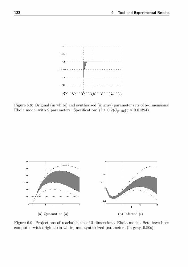
122 6. Tool and Experimental Results
Figure 6.8: Original (in white) and synthesized (in gray) parameter sets of 5-dimensionalEbola model with 2 parameters. Specification: (i ≤ 0.2)U[7,10](q ≤ 0.01394).
(a) Quarantine (q) (b) Infected (i)
Figure 6.9: Projections of reachable set of 5-dimensional Ebola model. Sets have beencomputed with original (in white) and synthesized parameters (in gray, 0.50s).
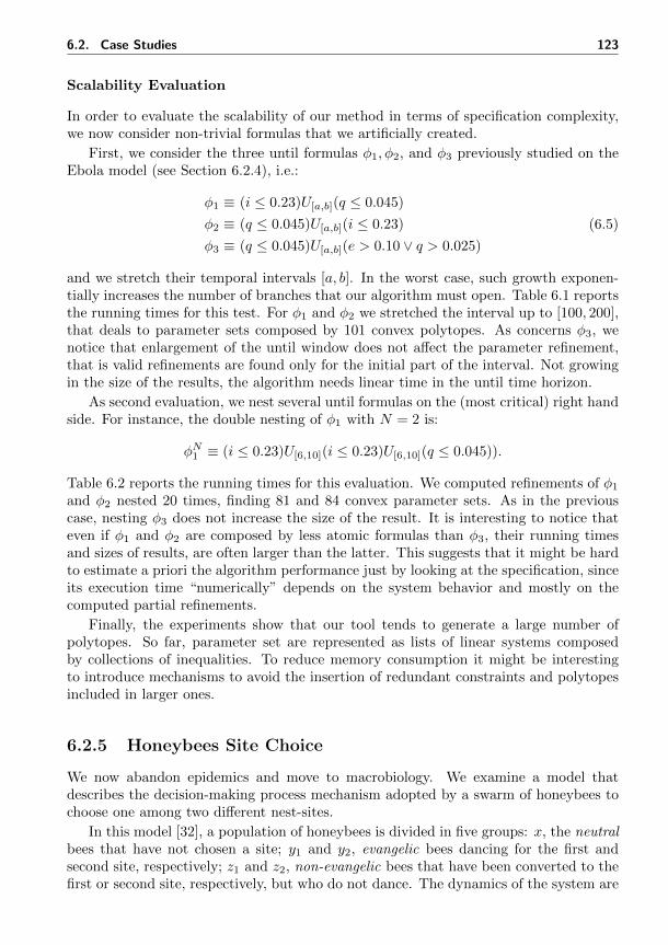
6.2. Case Studies 123
Scalability Evaluation
In order to evaluate the scalability of our method in terms of specification complexity,we now consider non-trivial formulas that we artificially created.
First, we consider the three until formulas φ1, φ2, and φ3 previously studied on theEbola model (see Section 6.2.4), i.e.:
φ1 ≡ (i ≤ 0.23)U[a,b](q ≤ 0.045)
φ2 ≡ (q ≤ 0.045)U[a,b](i ≤ 0.23)
φ3 ≡ (q ≤ 0.045)U[a,b](e > 0.10 ∨ q > 0.025)
(6.5)
and we stretch their temporal intervals [a, b]. In the worst case, such growth exponen-tially increases the number of branches that our algorithm must open. Table 6.1 reportsthe running times for this test. For φ1 and φ2 we stretched the interval up to [100, 200],that deals to parameter sets composed by 101 convex polytopes. As concerns φ3, wenotice that enlargement of the until window does not affect the parameter refinement,that is valid refinements are found only for the initial part of the interval. Not growingin the size of the results, the algorithm needs linear time in the until time horizon.
As second evaluation, we nest several until formulas on the (most critical) right handside. For instance, the double nesting of φ1 with N = 2 is:
φN1 ≡ (i ≤ 0.23)U[6,10](i ≤ 0.23)U[6,10](q ≤ 0.045)).
Table 6.2 reports the running times for this evaluation. We computed refinements of φ1and φ2 nested 20 times, finding 81 and 84 convex parameter sets. As in the previouscase, nesting φ3 does not increase the size of the result. It is interesting to notice thateven if φ1 and φ2 are composed by less atomic formulas than φ3, their running timesand sizes of results, are often larger than the latter. This suggests that it might be hardto estimate a priori the algorithm performance just by looking at the specification, sinceits execution time “numerically” depends on the system behavior and mostly on thecomputed partial refinements.
Finally, the experiments show that our tool tends to generate a large number ofpolytopes. So far, parameter set are represented as lists of linear systems composedby collections of inequalities. To reduce memory consumption it might be interestingto introduce mechanisms to avoid the insertion of redundant constraints and polytopesincluded in larger ones.
6.2.5 Honeybees Site Choice
We now abandon epidemics and move to macrobiology. We examine a model thatdescribes the decision-making process mechanism adopted by a swarm of honeybees tochoose one among two different nest-sites.
In this model [32], a population of honeybees is divided in five groups: x, the neutralbees that have not chosen a site; y1 and y2, evangelic bees dancing for the first andsecond site, respectively; z1 and z2, non-evangelic bees that have been converted to thefirst or second site, respectively, but who do not dance. The dynamics of the system are
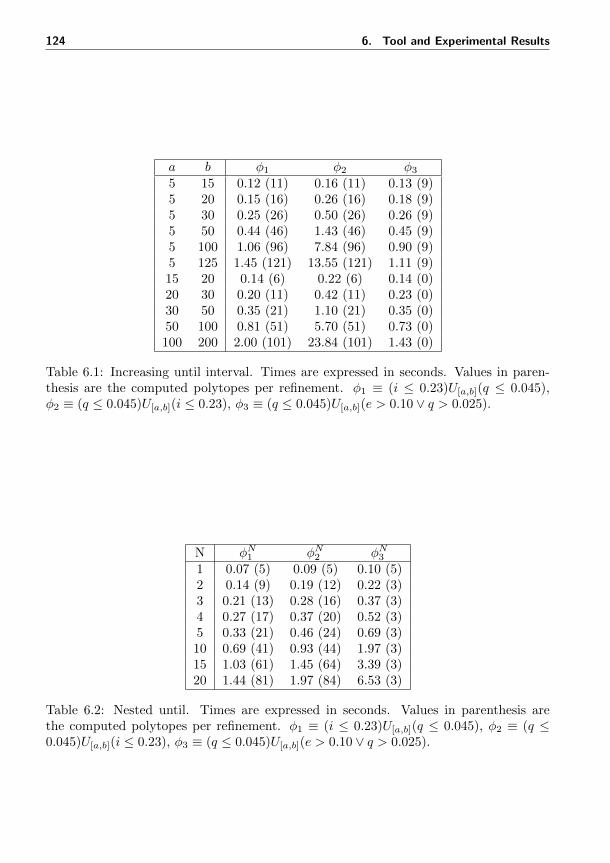
124 6. Tool and Experimental Results
a b φ1 φ2 φ35 15 0.12 (11) 0.16 (11) 0.13 (9)5 20 0.15 (16) 0.26 (16) 0.18 (9)5 30 0.25 (26) 0.50 (26) 0.26 (9)5 50 0.44 (46) 1.43 (46) 0.45 (9)5 100 1.06 (96) 7.84 (96) 0.90 (9)5 125 1.45 (121) 13.55 (121) 1.11 (9)15 20 0.14 (6) 0.22 (6) 0.14 (0)20 30 0.20 (11) 0.42 (11) 0.23 (0)30 50 0.35 (21) 1.10 (21) 0.35 (0)50 100 0.81 (51) 5.70 (51) 0.73 (0)100 200 2.00 (101) 23.84 (101) 1.43 (0)
Table 6.1: Increasing until interval. Times are expressed in seconds. Values in paren-thesis are the computed polytopes per refinement. φ1 ≡ (i ≤ 0.23)U[a,b](q ≤ 0.045),φ2 ≡ (q ≤ 0.045)U[a,b](i ≤ 0.23), φ3 ≡ (q ≤ 0.045)U[a,b](e > 0.10 ∨ q > 0.025).
N φN1 φN2 φN31 0.07 (5) 0.09 (5) 0.10 (5)2 0.14 (9) 0.19 (12) 0.22 (3)3 0.21 (13) 0.28 (16) 0.37 (3)4 0.27 (17) 0.37 (20) 0.52 (3)5 0.33 (21) 0.46 (24) 0.69 (3)10 0.69 (41) 0.93 (44) 1.97 (3)15 1.03 (61) 1.45 (64) 3.39 (3)20 1.44 (81) 1.97 (84) 6.53 (3)
Table 6.2: Nested until. Times are expressed in seconds. Values in parenthesis arethe computed polytopes per refinement. φ1 ≡ (i ≤ 0.23)U[a,b](q ≤ 0.045), φ2 ≡ (q ≤0.045)U[a,b](i ≤ 0.23), φ3 ≡ (q ≤ 0.045)U[a,b](e > 0.10 ∨ q > 0.025).
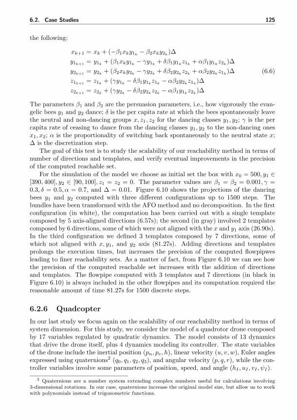
6.2. Case Studies 125
the following:
xk+1 = xk + (−β1xky1k − β2xky2k)∆
y1k+1= y1k + (β1xky1k − γy1k + δβ1y1kz1k + αβ1y1kz2k)∆
y2k+1= y2k + (β2xky2k − γy2k + δβ2y2kz2k + αβ2y2kz1k)∆
z1k+1= z1k + (γy1k − δβ1y1kz1k − αβ2y2kz1k)∆
z2k+1= z2k + (γy2k − δβ2y2kz2k − αβ1y1kz2k)∆
(6.6)
The parameters β1 and β2 are the persuasion parameters, i.e., how vigorously the evan-gelic bees y1 and y2 dance; δ is the per capita rate at which the bees spontaneously leavethe neutral and non-dancing groups x, z1, z2 for the dancing classes y1, y2; γ is the percapita rate of ceasing to dance from the dancing classes y1, y2 to the non-dancing onesx1, x2; α is the proportionality of switching back spontaneously to the neutral state x;∆ is the discretization step.
The goal of this test is to study the scalability of our reachability method in terms ofnumber of directions and templates, and verify eventual improvements in the precisionof the computed reachable set.
For the simulation of the model we choose as initial set the box with x0 = 500, y1 ∈[390, 400], y2 ∈ [90, 100], z1 = z2 = 0. The parameter values are β1 = β2 = 0.001, γ =0.3, δ = 0.5, α = 0.7, and ∆ = 0.01. Figure 6.10 shows the projections of the dancingbees y1 and y2 computed with three different configurations up to 1500 steps. Thebundles have been transformed with the AFO method and no decomposition. In the firstconfiguration (in white), the computation has been carried out with a single templatecomposed by 5 axis-aligned directions (6.57s); the second (in gray) involved 2 templatescomposed by 6 directions, some of which were not aligned with the x and y1 axis (26.90s).In the third configuration we defined 3 templates composed by 7 directions, some ofwhich not aligned with x, y1, and y2 axis (81.27s). Adding directions and templatesprolongs the execution times, but increases the precision of the computed flowpipwesleading to finer reachability sets. As a matter of fact, from Figure 6.10 we can see howthe precision of the computed reachable set increases with the addition of directionsand templates. The flowpipe computed with 3 templates and 7 directions (in black inFigure 6.10) is always included in the other flowpipes and its computation required thereasonable amount of time 81.27s for 1500 discrete steps.
6.2.6 Quadcopter
In our last study we focus again on the scalability of our reachability method in terms ofsystem dimension. For this study, we consider the model of a quadrotor drone composedby 17 variables regulated by quadratic dynamics. The model consists of 13 dynamicsthat drive the drone itself, plus 4 dynamics modeling its controller. The state variablesof the drone include the inertial position (pn, pe, h), linear velocity (u, v, w), Euler anglesexpressed using quaternions2 (q0, q1, q2, q3), and angular velocity (p, q, r), while the con-troller variables involve some parameters of position, speed, and angle (hI , uI , vI , ψI).
2 Quaternions are a number system extending complex numbers useful for calculations involving3-dimensional rotations. In our case, quaternions increase the original model size, but allow us to workwith polynomials instead of trigonometric functions.
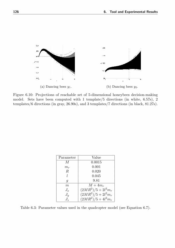
126 6. Tool and Experimental Results
(a) Dancing bees y1. (b) Dancing bees y2.
Figure 6.10: Projections of reachable set of 5-dimensional honeybees decision-makingmodel. Sets have been computed with 1 template/5 directions (in white, 6.57s), 2templates/6 directions (in gray, 26.90s), and 3 templates/7 directions (in black, 81.27s).
Parameter ValueM 0.0015mr 0.001R 0.020l 0.045g 9.81m M + 4mr
Jx (2MR2)/5 + 2l2mr
Jy (2MR2)/5 + 2l2mr
Jz (2MR2)/5 + 4l2mr
Table 6.3: Parameter values used in the quadcopter model (see Equation 6.7).
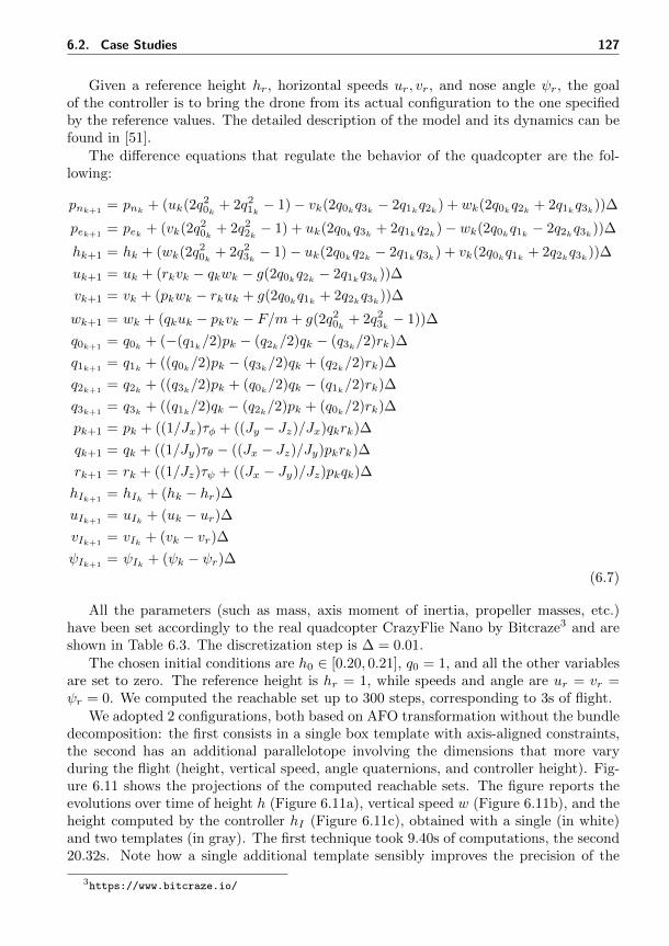
6.2. Case Studies 127
Given a reference height hr, horizontal speeds ur, vr, and nose angle ψr, the goalof the controller is to bring the drone from its actual configuration to the one specifiedby the reference values. The detailed description of the model and its dynamics can befound in [51].
The difference equations that regulate the behavior of the quadcopter are the fol-lowing:
pnk+1= pnk + (uk(2q20k + 2q21k − 1)− vk(2q0kq3k − 2q1kq2k) + wk(2q0kq2k + 2q1kq3k))∆
pek+1= pek + (vk(2q20k + 2q22k − 1) + uk(2q0kq3k + 2q1kq2k)− wk(2q0kq1k − 2q2kq3k))∆
hk+1 = hk + (wk(2q20k + 2q23k − 1)− uk(2q0kq2k − 2q1kq3k) + vk(2q0kq1k + 2q2kq3k))∆
uk+1 = uk + (rkvk − qkwk − g(2q0kq2k − 2q1kq3k))∆
vk+1 = vk + (pkwk − rkuk + g(2q0kq1k + 2q2kq3k))∆
wk+1 = wk + (qkuk − pkvk − F/m+ g(2q20k + 2q23k − 1))∆
q0k+1= q0k + (−(q1k/2)pk − (q2k/2)qk − (q3k/2)rk)∆
q1k+1= q1k + ((q0k/2)pk − (q3k/2)qk + (q2k/2)rk)∆
q2k+1= q2k + ((q3k/2)pk + (q0k/2)qk − (q1k/2)rk)∆
q3k+1= q3k + ((q1k/2)qk − (q2k/2)pk + (q0k/2)rk)∆
pk+1 = pk + ((1/Jx)τφ + ((Jy − Jz)/Jx)qkrk)∆
qk+1 = qk + ((1/Jy)τθ − ((Jx − Jz)/Jy)pkrk)∆
rk+1 = rk + ((1/Jz)τψ + ((Jx − Jy)/Jz)pkqk)∆
hIk+1= hIk + (hk − hr)∆
uIk+1= uIk + (uk − ur)∆
vIk+1= vIk + (vk − vr)∆
ψIk+1= ψIk + (ψk − ψr)∆
(6.7)
All the parameters (such as mass, axis moment of inertia, propeller masses, etc.)have been set accordingly to the real quadcopter CrazyFlie Nano by Bitcraze3 and areshown in Table 6.3. The discretization step is ∆ = 0.01.
The chosen initial conditions are h0 ∈ [0.20, 0.21], q0 = 1, and all the other variablesare set to zero. The reference height is hr = 1, while speeds and angle are ur = vr =ψr = 0. We computed the reachable set up to 300 steps, corresponding to 3s of flight.
We adopted 2 configurations, both based on AFO transformation without the bundledecomposition: the first consists in a single box template with axis-aligned constraints,the second has an additional parallelotope involving the dimensions that more varyduring the flight (height, vertical speed, angle quaternions, and controller height). Fig-ure 6.11 shows the projections of the computed reachable sets. The figure reports theevolutions over time of height h (Figure 6.11a), vertical speed w (Figure 6.11b), and theheight computed by the controller hI (Figure 6.11c), obtained with a single (in white)and two templates (in gray). The first technique took 9.40s of computations, the second20.32s. Note how a single additional template sensibly improves the precision of the
3https://www.bitcraze.io/
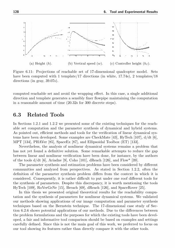
128 6. Tool and Experimental Results
(a) Height (h). (b) Vertical speed (w). (c) Controller height (hI).
Figure 6.11: Projections of reachable set of 17-dimensional quadcopter model. Setshave been computed with 1 template/17 directions (in white, 17.74s), 2 templates/18directions (in gray, 39.07s).
computed reachable set and avoid the wrapping effect. In this case, a single additionaldirection and template generates a sensibly finer flowpipe maintaining the computationin a reasonable amount of time (20.32s for 300 discrete steps).
6.3 Related Tools
In Sections 1.2.1 and 1.2.2 we presented some of the existing techniques for the reach-able set computation and the parameter synthesis of dynamical and hybrid systems.As pointed out, efficient methods and tools for the verification of linear dynamical sys-tems have been developed. Some examples are CheckMate [43], HyTech [107], d/dt [6],MPT [134], PHAVer [85], SpaceEx [87], and Ellipsoidal Toolbox (ET) [133].
Nevertheless, the analysis of nonlinear dynamical systems remains a problem thathas not yet found a definitive solution. Some remarkable attempts to reduce the gapbetween linear and nonlinear verification have been done, for instance, by the authorsof the tools d/dt [6], Ariadne [9], Coho [101], dReach [126], and Flow* [39].
The parameter synthesis and estimation problems have been considered by differentcommunities and analyzed from perspectives. As stated in Section 1.2.2, often thedefinition of the parameter synthesis problem differs from the context in which it isconsidered. Consequently, it is rather difficult to put under one roof different tools forthe synthesis of parameters. Despite this discrepancy, it is worth mentioning the toolsHyTech [109], RoVerGeNe [15], Breach [69], dReach [126], and SpaceRover [25].
In this thesis we presented original theoretical results for the reachability compu-tation and the synthesis of parameters for nonlinear dynamical systems. We validatedour methods showing applications of our image computation and parameter synthesistechniques based on the Bernstein technique. The 17-dimensional case study of Sec-tion 6.2.6 shows potential applications of our methods. Due to the differences betweenthe problem formulations and the purposes for which the existing tools have been devel-oped, a fair and informative tool comparison should be based on examples and settingscarefully defined. Since this is not the main goal of this work, we preferred to focus onour tool showing its features rather than directly compare it with the other tools.
7Conclusion
7.1 Thesis Overview
With this thesis we contributed to the development of theoretical and practical tech-niques for the analysis of discrete-time dynamical systems.
Our theoretical results involve the reachable set computation and the synthesisof parameters. Concerning reachability computation, we developed methods to over-approximate the images of sets with respects to polynomial functions (Chapter 4). Setsto be transformed can be over-approximated using boxes (Section 4.3), parallelotopes(Section 4.4), and our new data structure called parallelotope bundles (Section 4.5), thatcan be used to represent polytopes as intersections of parallelotopes. All these methodsare based on the representation of polynomials in Bernstein basis, and in particular onBernstein coefficients and their properties. We introduced new methods to efficientlycompute Bernstein coefficients and improve the bounds that they provide (Section 4.6).
Regarding parameter synthesis, we formalized the problem from a formal verificationperspective involving the Signal Temporal Logic (STL) for the characterization of thespecifications that the system must meet. We developed a new semantics for STL,called synthesis semantics, suitable for working with flowpipes and sets of parameters(Section 5.2). We defined an algorithm to compute the synthesis semantics of STLspecifications and obtain valid sets of parameters for discrete-time dynamical systems(Section 5.3). We also provided an instantiation of our synthesis algorithm for dynamicalsystems with polynomial dynamics, in which the reachable set can be approximated withboxes or parallelotopes, while parameter sets are represent by polytopes (Section 5.4).The synthesis technique broadly consists in the resolution of linear programs involving,also in this case, Bernstein coefficients.
From the practical point of view, we implemented a tool called Sapo that integratesall the techniques developed in work (Section 6.1). Sapo can be either used to com-pute flowpipes that over-approximate the reachable sets of dynamical systems, or tosynthesize sets of parameters with respect to STL specifications. We shown the effec-tiveness of our tool and analyzed its performances on several case studies coming fromepidemiology, macrobiology, and embedded systems (Section 6.2).
130 7. Conclusion
7.2 Further Developments
There are several aspects of this work that can be further investigated.
Parallelization There are several stages of our methods that can be easily paral-lelized. For instance, the computation of Bernstein coefficients of the functions thatencode the lifting of a direction over a reached set, can be independently performed foreach direction of a box or parallelotope. Or else, when working with bundles, everyparallelotope can be independently treated, meaning that the bundle-based reachabilitymethod can be straightforwardly parallelized. Also, in a hypothetical error containmentapproach where the reachability computation or parameter synthesis problems are splitin several subproblems, each instance can be separately treated in parallel.
It might be interesting to investigate the parallelization of our methods exploitingsome environment for parallel computations (such as MPI [103] or CUDA [153]).
Error Approximation In Section 4.2.1 we have seen how the error between themaximum of a polynomial and its maximum Bernstein coefficient can be bound. Inthe bundle transformation we provided a heuristic to minimize this error. Moreover,in Section 4.5.2, we provided a subdivision method to obtain tight bounds. However,it remains the question of how automatically control the error introduced by Bernsteincoefficients in the image of sets and in the synthesis of parameters. One can imaginea procedure that automatically splits the Bernstein coefficients so that to maintain theerrors below a given threshold.
Since Bernstein coefficients are sensitive to the size of the set on which they areexploited, an additional technique to produce finer results, could consist in splitting thereachability and parameter sets. This approach could be integrated in a backtrackingalgorithm that, once it determines that the results are not enough precise, jumps backin the constructed flowpipe, splits the sets, solves the subproblems for the split sets, andfinally combines the results.
Input Synthesis The parameter synthesis methods developed in this work can beadapted to synthesize valid inputs for open dynamical systems.
A discrete-time dynamical system with inputs can be described by difference equa-tions of the form:
xk+1 = f(xk,uk)
with f : Rn × Rm → Rn. Differently from parameters, inputs uk can change in a giveninput space U ⊆ Rm at every time step. The evolution x0,x1,x2, . . . of a dynamicalsystem with inputs starts from an initial condition x0 and it is driven by a sequence ofinputs u0,u1,u2, . . . .
The input synthesis problem asks to determine a sequence of input sets U0, U1, U2, . . . ,with Ui ⊆ U , that leads to a flowpipe of inputs, such that all the trajectories startingin a given set of initial conditions X0 with input sequence u0,u1,u2, . . . , with ui ∈ Ui,satisfy a given specification.
Our parameter refinements can be used for input synthesis. Instead of accumulatinga sequence of restrictions on the initial set to refine (in the case of parameter synthesis,the set P ), at each step we can independently compute a refined set of inputs Ui ⊆
7.2. Further Developments 131
U , producing a flowpipe of inputs U0, U1, U2, . . . so that the system satisfies a givenspecification.
Hybrid Automata Verification In this thesis we considered the computation ofthe reachable set of dynamical systems. A natural extension of this work could involvehybrid automata, that are mathematical models particularly suitable for the descriptionof systems that exhibit discrete and continuous behaviors.
Intuitively, hybrid automata are directed graphs with decorated nodes and edges.Each node of the graph, often called mode or location, is equipped with a dynamicalsystem (usually a set of difference or differential equations) that drives the system withina mode. Edges are decorated with activation and reset constraints that tell the systemwhen a discrete transition between modes can occur, and with which values the systemis reset once it jumps from a mode to another one.
The verification of hybrid automata with nonlinear dynamics is a difficult problemfor which not many efficient methods have been developed (in comparison with those forthe linear case; see Section 1.2.1 for an overview on the existing nonlinear reachabilitymethods). The set image computation techniques developed in this work could beused to compute the reachable set of hybrid automata with polynomial dynamics: theevolutions within modes could be directly carried out applying our reachability methods;the activations would require the intersection between sets (here some attention shouldbe placed on the sets described by the activations); the reset would consist in a singleset image computable with one of our techniques (assuming that the reset function ispolynomial).

Bibliography
[1] Linda JS Allen. Some discrete-time si, sir, and sis epidemic models. Mathematicalbiosciences, 124(1):83–105, 1994.
[2] Matthias Althoff and Bruce H Krogh. Zonotope bundles for the efficient compu-tation of reachable sets. In Conference on Decision and Control and EuropeanControl Conference, CDC-ECC, pages 6814–6821. IEEE, 2011.
[3] Matthias Althoff, Colas Le Guernic, and Bruce H Krogh. Reachable set computa-tion for uncertain time-varying linear systems. In Hybrid Systems: Computationand Control, HSCC, pages 93–102. ACM, 2011.
[4] Hirokazu Anai and Volker Weispfenning. Reach set computations using real quan-tifier elimination. In Hybrid Systems: Computation and Control, HSCC, pages63–76, 2001.
[5] Yashwanth Annpureddy, Che Liu, Georgios E. Fainekos, and Sriram Sankara-narayanan. S-TaLiRo: A tool for temporal logic falsification for hybrid systems.In Tools and Algorithms for the Construction and Analysis of Systems, TACAS,pages 254–257, 2011.
[6] Eugene Asarin, Olivier Bournez, Thao Dang, and Oded Maler. Approximatereachability analysis of piecewise-linear dynamical systems. In Hybrid Systems:Computation and Control, HSCC, pages 20–31. Springer, 2000.
[7] Eugene Asarin, Alexandre Donze, Oded Maler, and Dejan Nickovic. Parametricidentification of temporal properties. In Runtime Verification, RV, pages 147–160.Springer-Verlag, 2012.
[8] M. Avriel. Nonlinear Programming: Analysis and Methods. Dover Books onComputer Science Series. Dover Publications, 2003.
[9] Andrea Balluchi, Alberto Casagrande, Pieter Collins, Alberto Ferrari, TizianoVilla, and Alberto L Sangiovanni-Vincentelli. Ariadne: a framework for reach-ability analysis of hybrid automata. In Mathematical Theory of Networks andSystems, MTNS. Citeseer, 2006.
[10] Jiri Barnat, Lubos Brim, Adam Krejci, Adam Streck, David Safranek, MartinVejnar, and Tomas Vejpustek. On parameter synthesis by parallel model checking.IEEE/ACM Trans. Comput. Biology Bioinform., 9(3):693–705, 2012.
134 Bibliography
[11] Ezio Bartocci, Luca Bortolussi, and Laura Nenzi. On the robustness of temporalproperties for stochastic models. In Hybrid Systems and Biology, HSB, volume125 of EPTCS, pages 3–19, 2013.
[12] Ezio Bartocci, Luca Bortolussi, Laura Nenzi, and Guido Sanguinetti. On therobustness of temporal properties for stochastic models. In Hybrid Systems andBiology, HSB, pages 3–19, 2013.
[13] Gregory Batt, Calin Belta, and Ron Weiss. Model checking genetic regulatory net-works with parameter uncertainty. In Hybrid Systems: Computation and Control,HSCC, pages 61–75, 2007.
[14] Gregory Batt, Calin Belta, and Ron Weiss. Model checking liveness properties ofgenetic regulatory networks. In Tools and Algorithms for the Construction andAnalysis of Systems, TACAS, pages 323–338, 2007.
[15] Gregory Batt, Calin Belta, and Ron Weiss. Temporal logic analysis of gene net-works under parameter uncertainty. IEEE Trans. Automat. Contr., 53:215–229,2008.
[16] Gregory Batt, Michel Page, Irene Cantone, Gregor Goessler, Pedro T. Monteiro,and Hidde de Jong. Efficient parameter search for qualitative models of regulatorynetworks using symbolic model checking. Bioinformatics, 26(18), 2010.
[17] Gregory Batt, Delphine Ropers, Hidde de Jong, Johannes Geiselmann, Radu Ma-teescu, Michel Page, and Dominique Schneider. Analysis and verification of qual-itative models of genetic regulatory networks: A model-checking approach. InInternational Joint Conference on Artificial Intelligence, IJCAI, pages 370–375,2005.
[18] Gregory Batt, Boyan Yordanov, Ron Weiss, and Calin Belta. Robustness analysisand tuning of synthetic gene networks. Bioinformatics, 23(18):2415–2422, 2007.
[19] Christian Bauer, Alexander Frink, and Richard Kreckel. Introduction to theGiNaC framework for symbolic computation within the C++ programming lan-guage. Journal of Symbolic Computation, 33(1):1–12, 2002.
[20] Spring Berman, Adam Halasz, and Vijay Kumar. Marco: a reachability algorithmfor multi-affine systems with applications to biological systems. In Hybrid Systems:Computation and Control, HSCC, pages 76–89. Springer, 2007.
[21] Sergei Natanovich Bernstein. Demonstration du theoreme de weierstrass fondeesur le calcul des probabilites. Communications de la Societe Mathematique deKharkov 2, 1(4/5):1–2, 1912.
[22] Martin Berz and Kyoko Makino. Verified integration of odes and flows usingdifferential algebraic methods on high-order taylor models. Reliable Computing,4(4):361–369, 1998.
Bibliography 135
[23] Sergiy Bogomolov, Thomas A. Henzinger, Andreas Podelski, Jakob Ruess, andChristian Schilling. Adaptive moment closure for parameter inference of biochem-ical reaction networks. In Computational Methods in Systems Biology, CMSB,pages 77–89, 2015.
[24] Sergiy Bogomolov, Christian Schilling, Ezio Bartocci, Gregory Batt, Hui Kong,and Radu Grosu. Abstraction-based parameter synthesis for multiaffine systems.In Hardware and Software: Verification and Testing, Haifa Verification Confer-ence, HVC, pages 19–35, 2015.
[25] Sergiy Bogomolov, Christian Schilling, Ezio Bartocci, Gregory Batt, AndreasPodelski, and Radu Grosu. Spacerover: Parameter synthesis for multiaffine sys-tems beyond RoVerGeNe. To appear, 2015.
[26] Luca Bortolussi and Guido Sanguinetti. A statistical approach for computingreachability of non-linear and stochastic dynamical systems. In Quantitative Eval-uation of Systems, QEST, pages 41–56, 2014.
[27] Oleg Botchkarev and Stavros Tripakis. Verification of hybrid systems with lin-ear differential inclusions using ellipsoidal approximations. In Hybrid Systems:Computation and Control, HSCC, pages 73–88. Springer, 2000.
[28] Olivier Bournez, Oded Maler, and Amir Pnueli. Orthogonal polyhedra: Represen-tation and computation. In Hybrid Systems: Computation and Control, HSCC,pages 46–60. Springer, 1999.
[29] Lubos Brim, Milan Ceska, Martin Demko, Samuel Pastva, and David Safranek.Parameter synthesis by parallel coloured CTL model checking. In ComputationalMethods in Systems Biology, CMSB, pages 251–263, 2015.
[30] Lubos Brim, Milan Ceska, and David Safranek. Model checking of biologicalsystems. In Formal Methods for Dynamical Systems, SFM, pages 63–112, 2013.
[31] M. Brin and G. Stuck. Introduction to Dynamical Systems. Cambridge UniversityPress, 2002.
[32] NF Britton, NR Franks, SC Pratt, and TD Seeley. Deciding on a new home:how do honeybees agree? Royal Society of London B: Biological Sciences,269(1498):1383–1388, 2002.
[33] Christopher W. Brown. QEPCAD B: A program for computing with semi-algebraic sets using CADs. SIGSAM BULLETIN, 37:97–108, 2003.
[34] Laurence Calzone, Francois Fages, and Sylvain Soliman. BIOCHAM: an envi-ronment for modeling biological systems and formalizing experimental knowledge.Bioinformatics, 22(14):1805–1807, 2006.
[35] Alberto Casagrande and Tommaso Dreossi. pyhybrid analysis: A package forsemantics analysis of hybrid systems. In Euromicro Conference on Digital SystemDesign, DSD, pages 815–818, 2013.

136 Bibliography
[36] Alberto Casagrande, Tommaso Dreossi, Jana Fabrikova, and Carla Piazza. ε-semantics computations on biological systems. Inf. Comput., 236:35–51, 2014.
[37] Xin Chen, Edo Abraham, and Sriram Sankaranarayanan. Taylor model flowpipeconstruction for non-linear hybrid systems. In Real-Time Systems Symposium,RTSS, pages 183–192. IEEE, 2012.
[38] Xin Chen, Erika Abraham, and Goran Frehse. Efficient bounded reachabilitycomputation for rectangular automata. In Reachability Problems, RP, pages 139–152, 2011.
[39] Xin Chen, Erika Abraham, and Sriram Sankaranarayanan. Flow*: An analyzer fornon-linear hybrid systems. In Computer Aided Verification, CAV, pages 258–263,2013.
[40] Gerardo Chowell, Nick W Hengartner, Carlos Castillo-Chavez, Paul W Fenimore,and JM Hyman. The basic reproductive number of Ebola and the effects of publichealth measures: the cases of Congo and Uganda. Journal of Theoretical Biology,229(1):119–126, 2004.
[41] Alongkrit Chutinan and Bruce H Krogh. Computing polyhedral approximationsto flow pipes for dynamic systems. In Conference on Decision and Control, CDC,volume 2, pages 2089–2094. IEEE, 1998.
[42] Alongkrit Chutinan and Bruce H Krogh. Computing approximating automatafor a class of linear hybrid systems. In Hybrid Systems V, pages 16–37. Springer,1999.
[43] Alongkrit Chutinan and Bruce H Krogh. Verification of polyhedral-invariant hy-brid automata using polygonal flow pipe approximations. In Hybrid Systems:Computation and Control, HSCC, pages 76–90. Springer, 1999.
[44] Vasek Chvatal. Linear programming. Macmillan, 1983.
[45] Eugenio Cinquemani, Andreas Milias-Argeitis, Sean Summers, and John Lygeros.Stochastic dynamics of genetic networks: modelling and parameter identification.Bioinformatics, 24(23):2748–2754, 2008.
[46] Edmund M Clarke, Orna Grumberg, and Doron Peled. Model checking. MITpress, 1999.
[47] George E Collins. Quantifier elimination for real closed fields by cylindrical alge-braic decompostion. In Automata Theory and Formal Languages, pages 134–183.Springer, 1975.
[48] Michael A Colon, Sriram Sankaranarayanan, and Henny B Sipma. Linear invariantgeneration using non-linear constraint solving. In Computer Aided Verification,CAV, pages 420–432. Springer, 2003.
Bibliography 137
[49] Patrick Cousot and Radhia Cousot. Abstract interpretation: a unified latticemodel for static analysis of programs by construction or approximation of fix-points. In SIGACT-SIGPLAN symposium on Principles of programming lan-guages, pages 238–252. ACM, 1977.
[50] Harold Scott Macdonald Coxeter. Regular polytopes. Courier Corporation, 1973.
[51] Antonio Eduardo Carrilho da Cunha. Benchmark: Quadrotor attitude control. InApplied Verification for Continuous and Hybrid Systems, ARCH, 2015.
[52] Thao Dang. Approximate reachability computation for polynomial systems. InHybrid Systems: Computation and Control, HSCC, pages 138–152. Springer, 2006.
[53] Thao Dang, Alexandre Donze, Oded Maler, and Noa Shalev. Sensitive state-spaceexploration. In Conference on Decision and Control, CDC, pages 4049–4054, 2008.
[54] Thao Dang, Tommaso Dreossi, and Carla Piazza. Parameter synthesis using par-allelotopic enclosure and applications to epidemic models. In Hybrid Systems andBiology, HSB, pages 67–82, 2014.
[55] Thao Dang, Tommaso Dreossi, and Carla Piazza. Parameter synthesis throughtemporal logic specifications. In International Synmposium on Formal Methods,FM, pages 213–230, 2015.
[56] Thao Dang and David Salinas. Image computation for polynomial dynamicalsystems using the Bernstein expansion. In Computer Aided Verification, CAV,pages 219–232. Springer, 2009.
[57] Thao Dang and Romain Testylier. Reachability analysis for polynomial dynamicalsystems using the Bernstein expansion. Reliable Computing, 17(2):128–152, 2012.
[58] Thi Xuan Thao Dang. Verification and synthesis of hybrid systems. PhD thesis,Institut National Polytechnique de Grenoble-INPG, 2000.
[59] Ben D’Angelo, Sriram Sankaranarayanan, Cesar Sanchez, Will Robinson, BerndFinkbeiner, Henny B. Sipma, Sandeep Mehrotra, and Zohar Manna. LOLA: run-time monitoring of synchronous systems. In Temporal Representation and Rea-soning, TIME, pages 166–174, 2005.
[60] George B Dantzig and Mukund N Thapa. Linear programming 2: theory andextensions. Springer Science & Business Media, 2006.
[61] Philip J Davis and Philip Rabinowitz. Methods of numerical integration. CourierCorporation, 2007.
[62] Giuseppe De Giacomo and Moshe Y Vardi. Linear temporal logic and lineardynamic logic on finite traces. In International Joint Conference on ArtificialIntelligence, IJCAI, pages 854–860. AAAI Press, 2013.
[63] Leonardo De Moura and Nikolaj Bjørner. Z3: An efficient smt solver. In Tools andAlgorithms for the Construction and Analysis of Systems, TACAS, pages 337–340.Springer, 2008.
138 Bibliography
[64] Andreas Dolzmann and Thomas Sturm. REDLOG computer algebra meets com-puter logic. ACM SIGSAM Bulletin, 31:2–9, 1996.
[65] M.M. Donahue, G.T. Buzzard, and A.E. Rundell. Robust parameter identificationwith adaptive sparse grid-based optimization for nonlinear systems biology models.In American Control Conference, ACC, pages 5055–5060, June 2009.
[66] Robin Donaldson and David R. Gilbert. A model checking approach to the param-eter estimation of biochemical pathways. In Computational Methods in SystemsBiology, CMSB, pages 269–287, 2008.
[67] A. Donze. Trajectory-Based Verification and Controller Synthesis for Continuousand Hybrid Systems. PhD thesis, 2007.
[68] A. Donze, E. Fanchon, L. M. Gattepaille, O. Maler, and P. Tracqui. Robustnessanalysis and behavior discrimination in enzymatic reaction networks. PLOS One,6(9):e24246, 2011.
[69] Alexandre Donze. Breach, a toolbox for verification and parameter synthesis ofhybrid systems. In Computer Aided Verification, CAV, pages 167–170. Springer,2010.
[70] Alexandre Donze, Gilles Clermont, and Christopher James Langmead. Parametersynthesis in nonlinear dynamical systems: Application to systems biology. Journalof Computational Biology, 17(3):325–336, 2010.
[71] Alexandre Donze, Thomas Ferrere, and Oded Maler. Efficient robust monitoringfor stl. In Computer Aided Verification, CAV, pages 264–279. Springer, 2013.
[72] Alexandre Donze and Oded Maler. Systematic simulation using sensitivity anal-ysis. In Hybrid Systems: Computation and Control, HSCC, pages 174–189, 2007.
[73] Tommaso Dreossi and Thao Dang. Parameter synthesis for polynomial biologicalmodels. In Hybrid Systems: Computation and Control, HSCC, pages 233–242,2014.
[74] Tommaso Dreossi, Thao Dang, Alexandre Donze, James Kapinski, Xiaoqing Jin,and Jyotirmoy V. Deshmukh. Efficient guiding strategies for testing of temporalproperties of hybrid systems. In NASA Formal Method, NFM, pages 127–142,2015.
[75] Tommaso Dreossi, Thao Dang, and Carla Piazza. Parallelotope bundles for poly-nomial reachability. In Hybrid Systems: Computation and Control, HSCC, 2016.to appear.
[76] Freeman Dyson. A meeting with Enrico Fermi. Nature, 427(6972):297–297, 2004.
[77] Andreas Eggers, Nacim Ramdani, Nedialko S Nedialkov, and Martin Franzle.Improving the sat modulo ode approach to hybrid systems analysis by combiningdifferent enclosure methods. Software & Systems Modeling, 14(1):121–148, 2012.
Bibliography 139
[78] Georgios E. Fainekos, Antoine Girard, and George J. Pappas. Temporal logicverification using simulation. In Formal Modeling and Analysis of Timed Systems,FORMATS, pages 171–186, 2006.
[79] Georgios E. Fainekos and George J. Pappas. Robustness of temporal logic specifi-cations for continuous-time signals. Theoretical Computer Science, 410(42):4262–4291, 2009.
[80] Georgios E Fainekos and George J Pappas. Robustness of temporal logic specifi-cations for continuous-time signals. Theoretical Computer Science, 410(42):4262–4291, 2009.
[81] Georgios E. Fainekos, Sriram Sankaranarayanan, Franjo Ivancic, and Aarti Gupta.Robustness of model-based simulations. In Real-Time Systems Symposium, RTSS,pages 345–354. IEEE Press, 2009.
[82] Gerald E Farin. Curves and surfaces for CAGD: a practical guide. Morgan Kauf-mann, 2002.
[83] Rida T. Farouki. The Bernstein polynomial basis: a centennial retrospective.Computer Aided Geometric Design, 29(6):379–419, 2012.
[84] Richard P Feynman. Simulating physics with computers. International journal oftheoretical physics, 21(6/7):467–488, 1982.
[85] Goran Frehse. Phaver: Algorithmic verification of hybrid systems past hytech.In Hybrid Systems: Computation and Control, HSCC, pages 258–273. Springer,2005.
[86] Goran Frehse, Sumit Kumar Jha, and Bruce H. Krogh. A counterexample-guidedapproach to parameter synthesis for linear hybrid automata. In Hybrid Systems:Computation and Control, HSCC, pages 187–200, 2008.
[87] Goran Frehse, Colas Le Guernic, Alexandre Donze, Scott Cotton, Rajarshi Ray,Olivier Lebeltel, Rodolfo Ripado, Antoine Girard, Thao Dang, and Oded Maler.Spaceex: Scalable verification of hybrid systems. In Computer Aided Verification,CAV, pages 379–395. Springer, 2011.
[88] Sicun Gao. Computable Analysis, Decision Procedures, and Hybrid Automata:A New Framework for the Formal Verification of Cyber-Physical Systems. PhDthesis, PhD thesis, Carnegie Mellon University, 2012.
[89] Jurgen Garloff. The Bernstein algorithm. Interval Computations, 2(6):154–168,1993.
[90] Jurgen Garloff and Andrew P Smith. Investigation of a subdivision based algo-rithm for solving systems of polynomial equations. Nonlinear Analysis: Theory,Methods & Applications, 47(1):167–178, 2001.
[91] Jurgen Garloff and Andrew P Smith. Solution of systems of polynomial equationsby using Bernstein expansion. Springer, 2001.
140 Bibliography
[92] R. Ghaemi and D. Del Vecchio. Evaluating the robustness of a biochemical networkmodel. In Conference on Decision and Control, CDC, pages 615–620, Dec 2007.
[93] Reza Ghaemi, Jing Sun, Pablo A Iglesias, and Domitilla Del Vecchio. A methodfor determining the robustness of bio-molecular oscillator models. BMC systemsbiology, 3(1):95, 2009.
[94] Michael E Gilpin. Do hares eat lynx? American Naturalist, pages 727–730, 1973.
[95] Frank Giordano, William P Fox, and Steven Horton. A first course in mathemat-ical modeling. Cengage Learning, 2013.
[96] Antoine Girard. Reachability of uncertain linear systems using zonotopes. InHybrid Systems: Computation and Control, HSCC, pages 291–305. Springer, 2005.
[97] Antoine Girard, Colas Le Guernic, and Oded Maler. Efficient computation ofreachable sets of linear time-invariant systems with inputs. In Hybrid Systems:Computation and Control, HSCC, pages 257–271. Springer, 2006.
[98] Antoine Girard and George J Pappas. Verification using simulation. In HybridSystems: Computation and Control, HSCC, pages 272–286. Springer, 2006.
[99] Antoine Girard and George J Pappas. Approximation metrics for discrete andcontinuous systems. IEEE Transactions on Automatic Control, 52(5):782–798,2007.
[100] Diana-Elena Gratie, Bogdan Iancu, and Ion Petre. ODE analysis of biologicalsystems. In Formal Methods for Dynamical Systems, SFM, pages 29–62, 2013.
[101] Mark R Greenstreet and Ian Mitchell. Reachability analysis using polygonal pro-jections. In Hybrid Systems: Computation and Control, HSCC, pages 103–116.Springer, 1999.
[102] D Yu Grigor’ev. Complexity of deciding tarski algebra. Journal of symbolic Com-putation, 5(1):65–108, 1988.
[103] William Gropp, Ewing Lusk, Nathan Doss, and Anthony Skjellum. A high-performance, portable implementation of the mpi message passing interface stan-dard. Parallel computing, 22(6):789–828, 1996.
[104] Ashutosh Kumar Gupta, Rupak Majumdar, and Andrey Rybalchenko. Fromtests to proofs. International Journal on Software Tools for Technology Trans-fer, 15(4):291–303, 2013.
[105] Ernst Hairer, Christian Lubich, and Gerhard Wanner. Geometric numerical in-tegration: structure-preserving algorithms for ordinary differential equations, vol-ume 31. Springer Science & Business Media, 2006.
[106] John Havlicek, Scott Little, Oded Maler, and Dejan Nickovic. Property-basedmonitoring of analog and mixed-signal systems. In Formal Modeling and Analysisof Timed Systems, FORMATS, pages 23–24, 2010.
Bibliography 141
[107] Thomas A Henzinger, Pei-Hsin Ho, and Howard Wong-Toi. Hytech: A modelchecker for hybrid systems. In Computer Aided Verification, CAV, pages 460–463.Springer, 1997.
[108] Thomas A Henzinger, Peter W Kopke, Anuj Puri, and Pravin Varaiya. What’sdecidable about hybrid automata? In Symposium on Theory of computing, STOC,pages 373–382. ACM, 1995.
[109] Thomas A. Henzinger and Howard Wong-Toi. Using hytech to synthesize controlparameters for a steam boiler. In Formal Methods for Industrial Applications,pages 265–282, London, UK, UK, 1996. Springer-Verlag.
[110] Francis Begnaud Hildebrand. Introduction to numerical analysis. Courier Corpo-ration, 1987.
[111] Frederick S Hillier. Introduction to operations research. Tata McGraw-Hill Edu-cation, 1995.
[112] Alan C Hindmarsh, Peter N Brown, Keith E Grant, Steven L Lee, Radu Serban,Dan E Shumaker, and Carol S Woodward. Sundials: Suite of nonlinear anddifferential/algebraic equation solvers. Transactions on Mathematical Software,TOMS, 31(3):363–396, 2005.
[113] Faraz Hussain, Sumit Kumar Jha, Susmit Jha, and Christopher James Langmead.Parameter discovery in stochastic biological models using simulated annealing andstatistical model checking. IJBRA, 10(4/5):519–539, 2014.
[114] Jean-Louis Imbert and Pascal Van Hentenryck. Redundancy elimination witha lexicographic solved form. Annals of Mathematics and Artificial Intelligence,17(1):85–106, 1996.
[115] X. Jin, A. Donze, J. V. Deshmukh, and S. A. Seshia. Mining requirements fromclosed-loop control models. In Hybrid Systems: Computation and Control, HSCC,pages 43–52. ACM, 2013.
[116] K. D. Jones, V. Konrad, and D. Nickovic. Analog property checkers: a DDR2case study. Formal Methods in System Design, 36(2):114–130, 2010.
[117] A Agung Julius and George J Pappas. Trajectory based verification using localfinite-time invariance. In Hybrid Systems: Computation and Control, HSCC, pages223–236. Springer, 2009.
[118] Rudolf Emil Kalman, Peter L Falb, and Michael A Arbib. Topics in mathematicalsystem theory, volume 33. McGraw-Hill New York, 1969.
[119] James Kapinski, Jyotirmoy V Deshmukh, Sriram Sankaranarayanan, and NikosArechiga. Simulation-guided lyapunov analysis for hybrid dynamical systems. InHybrid Systems: Computation and Control, HSCC, pages 133–142. ACM, 2014.
[120] Jim Kapinski, Bruce H Krogh, Oded Maler, and Olaf Stursberg. On systematicsimulation of open continuous systems. In Hybrid Systems: Computation andControl, HSCC, pages 283–297. Springer, 2003.
142 Bibliography
[121] Narendra Karmarkar. A new polynomial-time algorithm for linear programming.In Symposium on Theory of computing, STOC, pages 302–311. ACM, 1984.
[122] Mark H Karwan, Vahid Lotfi, Jan Telgen, and Stanley Zionts. Redundancy inmathematical programming: A state-of-the-art survey, volume 206. Springer Sci-ence & Business Media, 2012.
[123] William O Kermack and Anderson G McKendrick. A contribution to the mathe-matical theory of epidemics. In Royal Society of London A: Mathematical, Physicaland Engineering Sciences, volume 115, pages 700–721. The Royal Society, 1927.
[124] Jongrae Kim, Declan G Bates, Ian Postlethwaite, Lan Ma, and Pablo A Iglesias.Robustness analysis of biochemical network models. IEE Proceedings-SystemsBiology, 153(3):96–104, 2006.
[125] Sharon E Kingsland. Modeling nature. University of Chicago Press, 1995.
[126] Soonho Kong, Sicun Gao, Wei Chen, and Edmund Clarke. dreach: δ-reachabilityanalysis for hybrid systems. In Tools and Algorithms for the Construction andAnalysis of Systems, TACAS, pages 200–205. Springer, 2015.
[127] EK Kostousova. State estimation for dynamic systems via parallelotopes optimiza-tion and parallel computations. Optimization Methods and Software, 9(4):269–306,1998.
[128] E. K. Kostousovat. Control synthesis via parallelotopes: optimzation and parallelcompuations. Optimization Methods and Software, 4(14):267–310, 1 2001.
[129] Konstantinos Koutroumpas, Zoi Lygerou, and John Lygeros. Parameter iden-tification for a DNA replication model. In Conference on Bioinformatics andBioengineering, BIBE, pages 1–6, 2008.
[130] Arnold R Krommer. Numerical Integration: On Advanced Computer Systems,volume 848. Springer Science & Business Media, 1994.
[131] Alexander B. Kurzhanski and Pravin Varaiya. Ellipsoidal techniques for reachabil-ity analysis. In Hybrid Systems: Computation and Control, HSCC, pages 202–214,2000.
[132] Alexander B Kurzhanski and Pravin Varaiya. Ellipsoidal techniques for reacha-bility analysis: internal approximation. Systems & control letters, 41(3):201–211,2000.
[133] Alex A Kurzhanskiy, Pravin Varaiya, et al. Ellipsoidal toolbox. EECS Department,University of California, Berkeley, Tech. Rep. UCB/EECS-2006-46, 2006.
[134] Michal Kvasnica, Pascal Grieder, Mato Baotic, and Manfred Morari. Multi-parametric toolbox (mpt). In Hybrid Systems: Computation and Control, HSCC,pages 448–462. Springer, 2004.
Bibliography 143
[135] Gerardo Lafferriere, George J Pappas, and Sergio Yovine. Symbolic reachabilitycomputation for families of linear vector fields. Journal of Symbolic Computation,32(3):231–253, 2001.
[136] Jean-Louis Lassez, Tien Huynh, and Ken McAloon. Simplification and eliminationof redundant linear arithmetic constraints. Mit Press, 1993.
[137] Colas Le Guernic. Reachability analysis of hybrid systems with linear continuousdynamics. PhD thesis, Universite Joseph-Fourier-Grenoble I, 2009.
[138] Colas Le Guernic and Antoine Girard. Reachability analysis of linear systems usingsupport functions. Nonlinear Analysis: Hybrid Systems, 4(2):250–262, 2010.
[139] Gabriele Lillacci and Mustafa Khammash. Parameter estimation and model se-lection in computational biology. PLoS Comput Biol, 6(3):e1000696, 2010.
[140] Ernest Lindelof. Sur lapplication de la methode des approximations successivesaux equations differentielles ordinaires du premier ordre. Comptes rendus hebdo-madaires des seances de l’Academie des sciences, 114:454–457, 1894.
[141] Bing Liu, Soonho Kong, Sicun Gao, Paolo Zuliani, and Edmund M. Clarke. Pa-rameter synthesis for cardiac cell hybrid models using delta-decisions. CoRR,abs/1407.1524, 2014.
[142] Alfred Lotka. Elements of physical biology. 1925.
[143] Oded Maler and Dejan Nickovic. Monitoring temporal properties of continuous sig-nals. In Formal Techniques, Modelling and Analysis of Timed and Fault-TolerantSystems, pages 152–166. Springer, 2004.
[144] Oded Maler, Dejan Nickovic, and Amir Pnueli. Checking temporal propertiesof discrete, timed and continuous behaviors. Pillars of computer science, pages475–505, 2008.
[145] Jurgen Mayer, Khaled Khairy, and Jonathon Howard. Drawing an elephant withfour complex parameters. American Journal of Physics, 78(6):648–649, 2010.
[146] Pedro Mendes and D Kell. Non-linear optimization of biochemical pathways:applications to metabolic engineering and parameter estimation. Bioinformatics,14(10):869–883, 1998.
[147] Robin Milner. An Algebraic Definition of Simulation Between Programs. StanfordUniversity, Stanford, CA, USA, 1971.
[148] Robin Milner. Communication and Concurrency. Prentice-Hall, Inc., Upper Sad-dle River, NJ, USA, 1989.
[149] Marvin L Minsky. Computation: finite and infinite machines. Prentice-Hall, Inc.,1967.
[150] Carmen G Moles, Pedro Mendes, and Julio R Banga. Parameter estimation inbiochemical pathways: a comparison of global optimization methods. Genomeresearch, 13(11):2467–2474, 2003.
144 Bibliography
[151] Bernard Mourrain and Jean Pascal Pavone. Subdivision methods for solving poly-nomial equations. J. Symb. Comput., 44(3):292–306, 2009.
[152] PSV Nataraj and M Arounassalame. A new subdivision algorithm for the Bern-stein polynomial approach to global optimization. International journal of au-tomation and computing, 4(4):342–352, 2007.
[153] CUDA Nvidia. Programming guide, 2008.
[154] Sucheendra K. Palaniappan, Benjamin M. Gyori, Bing Liu, David Hsu, and P. S.Thiagarajan. Statistical model checking based calibration and analysis of bio-pathway models. In Computational Methods in Systems Biology, CMSB, pages120–134, 2013.
[155] David Park. Concurrency and automata on infinite sequences. Springer, 1981.
[156] P. A. Gonzlez Parra, S. Lee, L. Velzquez, and C. Castillo-Chavez. A note on the useof optimal control on a discrete time model of influenza dynamics. MathematicalBiosciences and Engineering, 8(1):183–197, 2011.
[157] Pablo A Parrilo. Semidefinite programming relaxations for semialgebraic prob-lems. Mathematical programming, 96(2):293–320, 2003.
[158] Pablo A Parrilo and Bernd Sturmfels. Minimizing polynomial functions. Al-gorithmic and quantitative real algebraic geometry, DIMACS Series in DiscreteMathematics and Theoretical Computer Science, 60:83–99, 2003.
[159] Carla Piazza, Marco Antoniotti, Venkatesh Mysore, Alberto Policriti, Franz Win-kler, and Bud Mishra. Algorithmic algebraic model checking i: Challenges fromsystems biology. In Computer Aided Verification, CAV, pages 5–19. Springer,2005.
[160] Andre Platzer. Differential dynamic logic for verifying parametric hybrid sys-tems. In Automated Reasoning with Analytic Tableaux and Related Methods,TABLEAUX, pages 216–232, 2007.
[161] Andre Platzer. Differential dynamic logic for hybrid systems. J. Autom. Reason-ing, 41(2):143–189, 2008.
[162] Andre Platzer and Jan-David Quesel. Keymaera: A hybrid theorem prover forhybrid systems (system description). In International Joint Conference on Auto-mated Reasoning, IJCAR, pages 171–178, 2008.
[163] Amir Pnueli. The temporal logic of programs. In Symposium on Foundations ofComputer Science, SFCS, pages 46–57. IEEE, 1977.
[164] Pavithra Prabhakar and Mahesh Viswanathan. A dynamic algorithm for approx-imate flow computations. In Hybrid Systems: Computation and Control, HSCC,HSCC ’11, pages 133–142, New York, NY, USA, 2011. ACM.
Bibliography 145
[165] Nacim Ramdani and Nedialko S Nedialkov. Computing reachable sets for uncer-tain nonlinear hybrid systems using interval constraint-propagation techniques.Nonlinear Analysis: Hybrid Systems, 5(2):149–162, 2011.
[166] Dietmar Ratz and Tibor Csendes. On the selection of subdivision directions ininterval branch-and-bound methods for global optimization. Journal of GlobalOptimization, 7(2):183–207, 1995.
[167] Shashwati Ray and PSV Nataraj. An efficient algorithm for range computation ofpolynomials using the Bernstein form. Journal of Global Optimization, 45(3):403–426, 2009.
[168] Shashwati Ray and PSV Nataraj. A matrix method for efficient computation ofbernstein coefficients. Reliable Computing, 17(1):40–71, 2012.
[169] Sriram Sankaranarayanan, Thao Dang, and Franjo Ivancic. Symbolic model check-ing of hybrid systems using template polyhedra. In Tools and Algorithms for theConstruction and Analysis of Systems, TACAS, pages 188–202. Springer, 2008.
[170] Sriram Sankaranarayanan, Henny B. Sipma, and Zohar Manna. Scalable anal-ysis of linear systems using mathematical programming. In Verification, ModelChecking, and Abstract Interpretation, VMCAI, pages 25–41, 2005.
[171] Mohamed Amin Ben Sassi and Sriram Sankaranarayanan. Bernstein poly-nomial relaxations for polynomial optimization problems. arXiv preprintarXiv:1509.01156, 2015.
[172] Mohamed Amin Ben Sassi, Sriram Sankaranarayanan, Xin Chen, and ErikaAbraham. Linear relaxations of polynomial positivity for polynomial lyapunovfunction synthesis. IMA Journal of Mathematical Control and Information, pagednv003, 2015.
[173] Hermann Schichl. Models and the history of modeling. In Josef Kallrath, editor,Modeling Languages in Mathematical Optimization, volume 88 of Applied Opti-mization, pages 25–36. Springer US, 2004.
[174] O Shisha. The Bernstein form of a polynomial. Journal of Research of the NationalBureau of Standards: Mathematics and mathematical physics. B, 70:79, 1966.
[175] Andrew Paul Smith. Enclosure Methods for Systems of Polynomial Equations andInequalities. PhD thesis, 2012.
[176] AndrewPaul Smith. Fast construction of constant bound functions for sparsepolynomials. Journal of Global Optimization, 43(2-3):445–458, 2009.
[177] S. Stoma, A. Donze, F. Bertaux, O. Maler, and G. Batt. STL-based Analysisof TRAIL-induced Apoptosis Challenges the Notion of Type I/Type II Cell LineClassification. PLoS Computational Biology, 9(5):e1003056, 2013.
[178] Olaf Stursberg and Bruce H Krogh. Efficient representation and computation ofreachable sets for hybrid systems. In Hybrid Systems: Computation and Control,HSCC, pages 482–497. Springer, 2003.
146 Bibliography
[179] Alfred Tarski. A decision method for elementary algebra and geometry. 1948,1951.
[180] Jan Telgen. Redundancy and linear programs. MC Tracts, 137:1–125, 1981.
[181] Romain Testylier. Reachability analysis of non-linear systems. PhD thesis, 2012.
[182] Ufuk Topcu, Andrew Packard, and Peter Seiler. Local stability analysis using sim-ulations and sum-of-squares programming. Automatica, 44(10):2669–2675, 2008.
[183] Ufuk Topcu, Andrew Packard, Peter Seiler, and Timothy Wheeler. Stability regionanalysis using simulations and sum-of-squares programming. In American ControlConference, ACC, pages 6009–6014. IEEE, 2007.
[184] Tayssir Touili, Byron Cook, and Paul Jackson, editors. Computer Aided Verifica-tion, CAV, volume 6174 of Lecture Notes in Computer Science. Springer, 2010.
[185] Pascal Van Hentenryck and Thomas Graf. Standard forms for rational lineararithmetic in constraint logic programming. Annals of Mathematics and ArtificialIntelligence, 5(2-4):303–319, 1992.
[186] Pravin Varaiya. Reach set computation using optimal control. In M.Kemal Inanand RobertP. Kurshan, editors, Verification of Digital and Hybrid Systems, volume170 of NATO ASI Series, pages 323–331. Springer Berlin Heidelberg, 2000.
[187] Vito Volterra. Variazioni e fluttuazioni del numero d’individui in specie animaliconviventi. C. Ferrari, 1927.
[188] J Wei. Least square fitting of an elephant. Chemtech, 5(2):128–129, 1975.
[189] Michael Zettler and Jurgen Garloff. Robustness analysis of polynomials withpolynomial parameter dependency using bernstein expansion. IEEE Transactionson Automatic Control, 43(3):425–431, 1998.
[190] Yan Zhang, Sriram Sankaranarayanan, Fabio Somenzi, Xin Chen, and ErikaAbraham. From statistical model checking to statistical model inference: charac-terizing the effect of process variations in analog circuits. In International Con-ference on Computer-Aided Design, ICCAD, pages 662–669, 2013.
[191] Xiaoliang Zhou, Xiaopei Li, and Wu-Sheng Wang. Bifurcations for a deterministicsir epidemic model in discrete time. Advances in Difference Equations, 2014(1):1–16, 2014.


![Polynomial-time Computation via Local Inference Relationsgivan/papers/tocl00.pdfF.1.1 [Mathematical Logic and Formal Languages] Models of Abstract Computation— computability theory;](https://img.pdfslide.us/doc/110x75/60295cbf6b7a1e587127ae94/polynomial-time-computation-via-local-inference-relations-givanpaperstocl00pdf.jpg)


![Masteroppgave i kryptografi - COnnecting REpositories · 2018-04-14 · Definition2.2(Polynomialparameter[3]). A parameter ais called a polynomial parameter if there exists a constant](https://img.pdfslide.us/doc/110x75/5f4b4997d5678f59a81330db/masteroppgave-i-kryptografi-connecting-repositories-2018-04-14-deinition22polynomialparameter3.jpg)