Embed Size (px)
Citation preview
Implementation Methods
Paulo Oliveira
Dynamic Stochastic Estimation, Prediction and Smoothing DEEC/SSC, Spring 2003
PhD. Programme
09/02/15 Paulo Oliveira 2
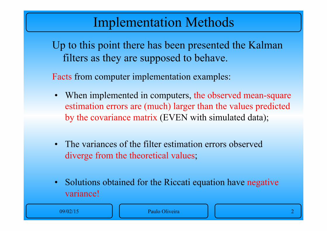
Implementation Methods Up to this point there has been presented the Kalman
filters as they are supposed to behave.
• When implemented in computers, the observed mean-square estimation errors are (much) larger than the values predicted by the covariance matrix (EVEN with simulated data);
• The variances of the filter estimation errors observed diverge from the theoretical values;
• Solutions obtained for the Riccati equation have negative variance!
Facts from computer implementation examples:
09/02/15 Paulo Oliveira 3
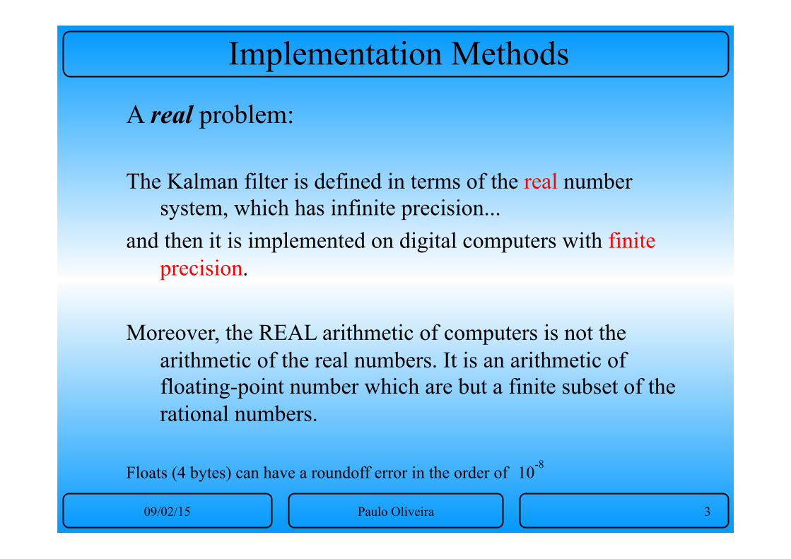
Implementation Methods
A real problem: The Kalman filter is defined in terms of the real number
system, which has infinite precision... and then it is implemented on digital computers with finite
precision. Moreover, the REAL arithmetic of computers is not the
arithmetic of the real numbers. It is an arithmetic of floating-point number which are but a finite subset of the rational numbers.
Floats (4 bytes) can have a roundoff error in the order of 10-8
09/02/15 Paulo Oliveira 4
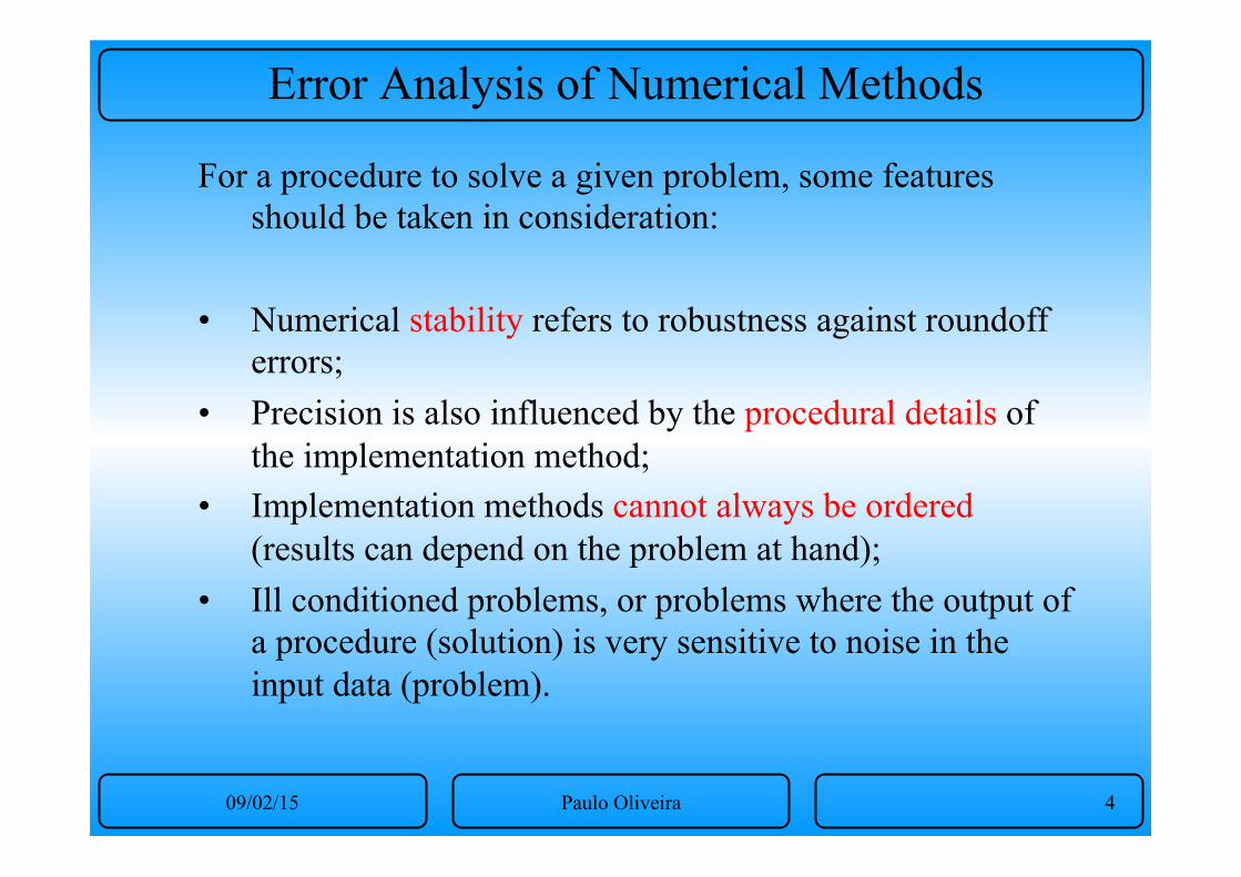
Error Analysis of Numerical Methods
For a procedure to solve a given problem, some features should be taken in consideration:
• Numerical stability refers to robustness against roundoff
errors; • Precision is also influenced by the procedural details of
the implementation method; • Implementation methods cannot always be ordered
(results can depend on the problem at hand); • Ill conditioned problems, or problems where the output of
a procedure (solution) is very sensitive to noise in the input data (problem).
09/02/15 Paulo Oliveira 5
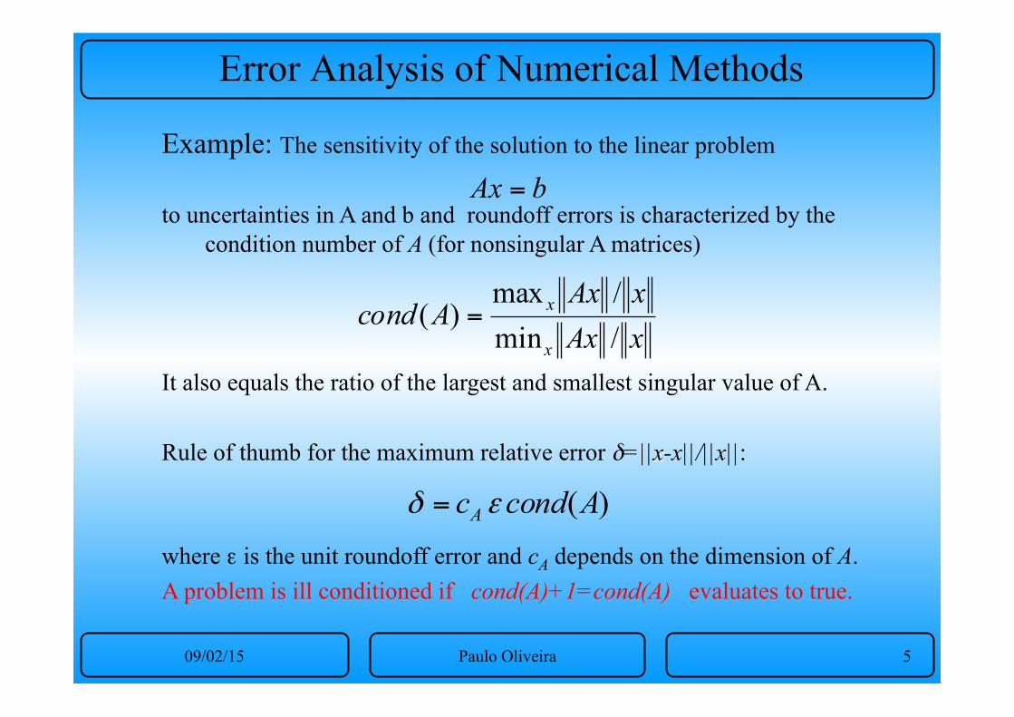
Error Analysis of Numerical Methods
Example: The sensitivity of the solution to the linear problem
to uncertainties in A and b and roundoff errors is characterized by the condition number of A (for nonsingular A matrices)
It also equals the ratio of the largest and smallest singular value of A. Rule of thumb for the maximum relative error δ=||x-x||/||x||: where ε is the unit roundoff error and cA depends on the dimension of A. A problem is ill conditioned if cond(A)+1=cond(A) evaluates to true.
bAx =
xAxxAx
Acondx
x
/min/max
)( =
)(AcondcAεδ =
09/02/15 Paulo Oliveira 6
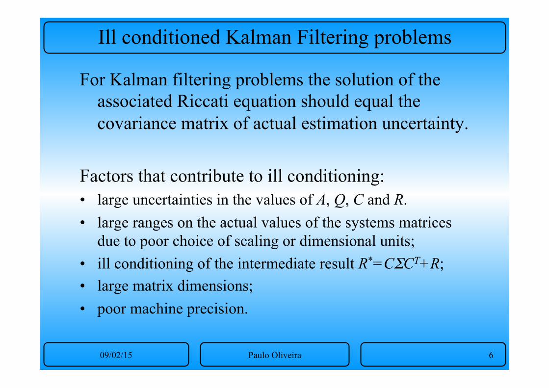
Ill conditioned Kalman Filtering problems
For Kalman filtering problems the solution of the associated Riccati equation should equal the covariance matrix of actual estimation uncertainty.
Factors that contribute to ill conditioning: • large uncertainties in the values of A, Q, C and R. • large ranges on the actual values of the systems matrices
due to poor choice of scaling or dimensional units; • ill conditioning of the intermediate result R*=CΣCT+R; • large matrix dimensions; • poor machine precision.
09/02/15 Paulo Oliveira 7
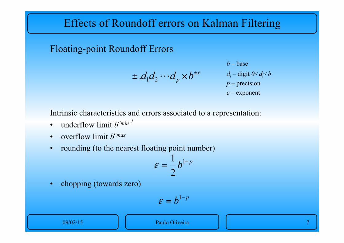
Effects of Roundoff errors on Kalman Filtering
Floating-point Roundoff Errors b – base di – digit 0<di<b p – precision e – exponent
Intrinsic characteristics and errors associated to a representation: • underflow limit bemin-1
• overflow limit bemax • rounding (to the nearest floating point number) • chopping (towards zero)
ep bddd ±×± !21.
pb −= 1
21
ε
pb −= 1ε
09/02/15 Paulo Oliveira 8
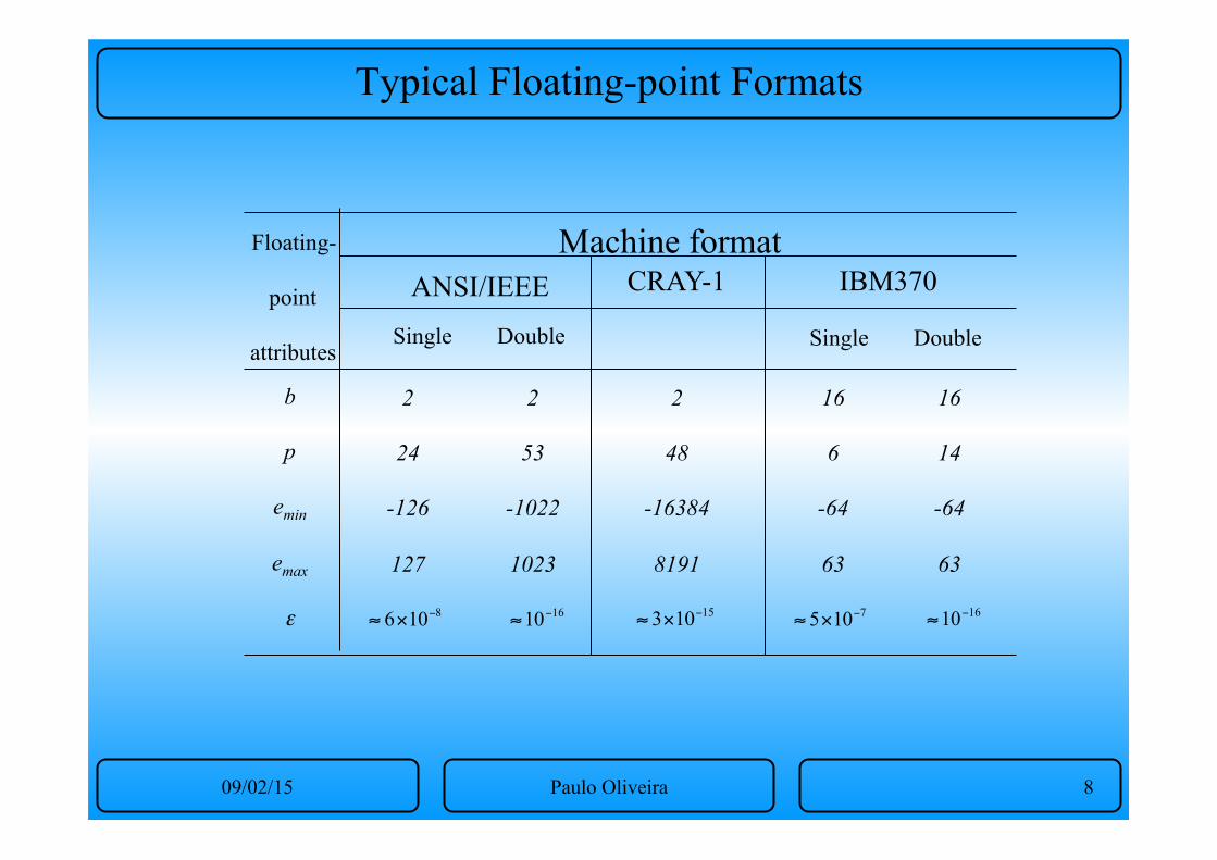
Typical Floating-point Formats
Machine format ANSI/IEEE CRAY-1 IBM370
Single Double Single Double
Floating-
point
attributes
b p
emin
emax ε
2 24
-126
127 8106 −×≈
2 53
-1022
1023 1610−≈
2 48
-16384
8191 15103 −×≈
16 6
-64 63 7105 −×≈
16 14
-64 63 1610−≈
09/02/15 Paulo Oliveira 9
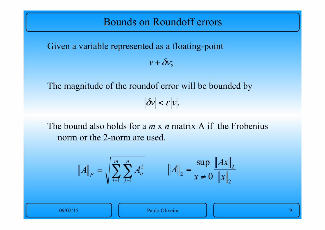
Bounds on Roundoff errors
Given a variable represented as a floating-point The magnitude of the roundof error will be bounded by The bound also holds for a m x n matrix A if the Frobenius
norm or the 2-norm are used.
;vv δ+
.vv εδ <
∑∑= =
=m
i
n
jijFAA
1 1
2
2
22 0
supxAx
xA
≠=
09/02/15 Paulo Oliveira 10
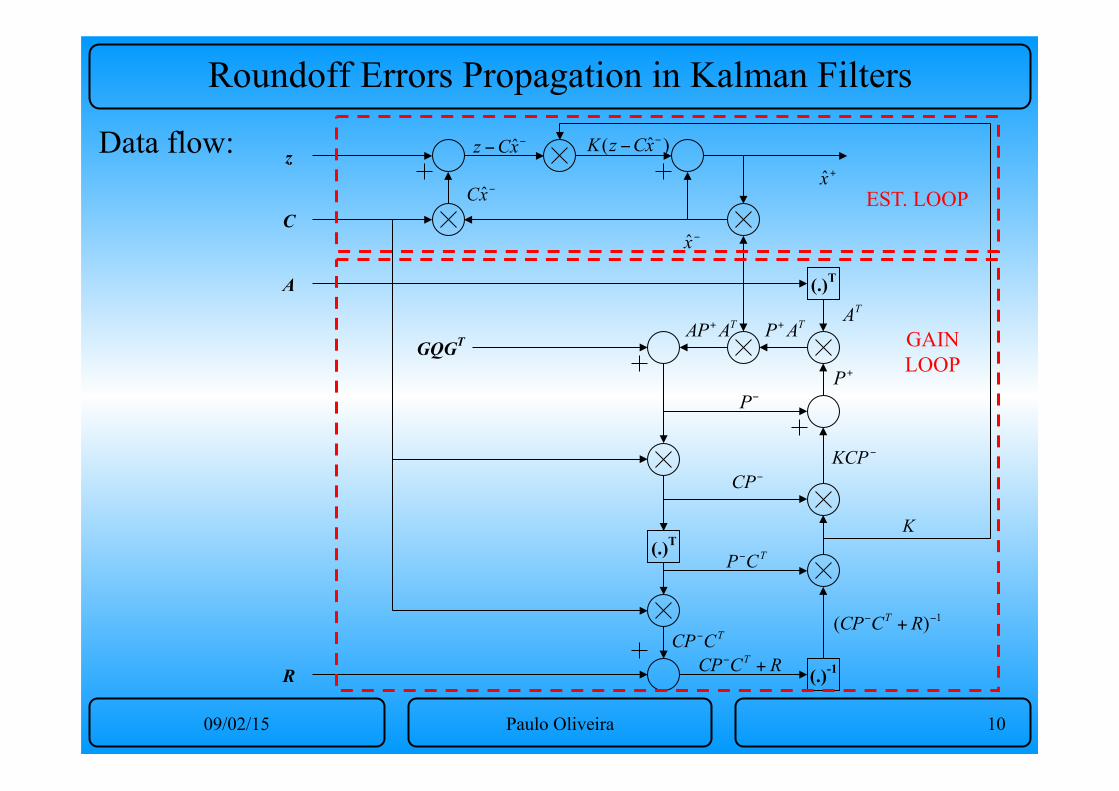
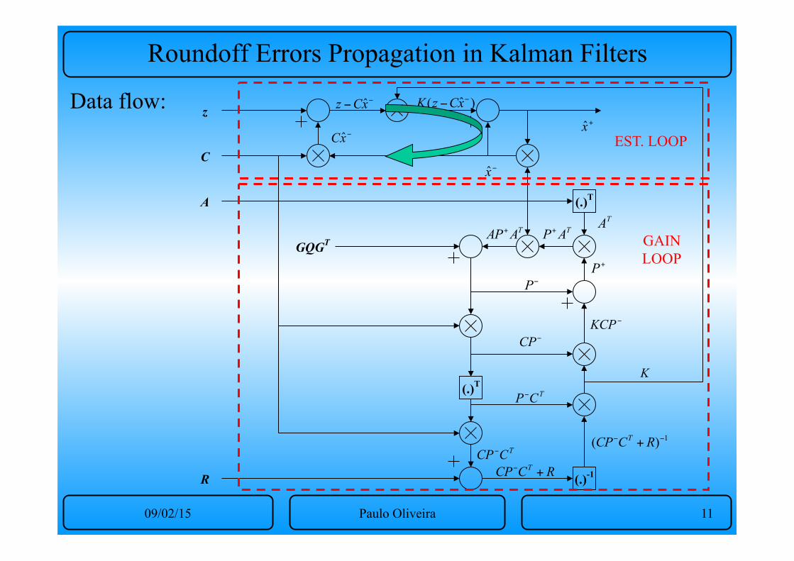
Roundoff Errors Propagation in Kalman Filters
Data flow:
(.)T
(.)T
(.)-1
z
C
A
GQGT
R
−− xCz ˆ )ˆ( −− xCzK
K
−x
−xC ˆ
TA
−P
+P
TAP+TAAP+
−CP
−KCP
TCP−
TCCP−
RCCP T +−
1)( −− + RCCP T
EST. LOOP
GAIN LOOP
+x
09/02/15 Paulo Oliveira 11
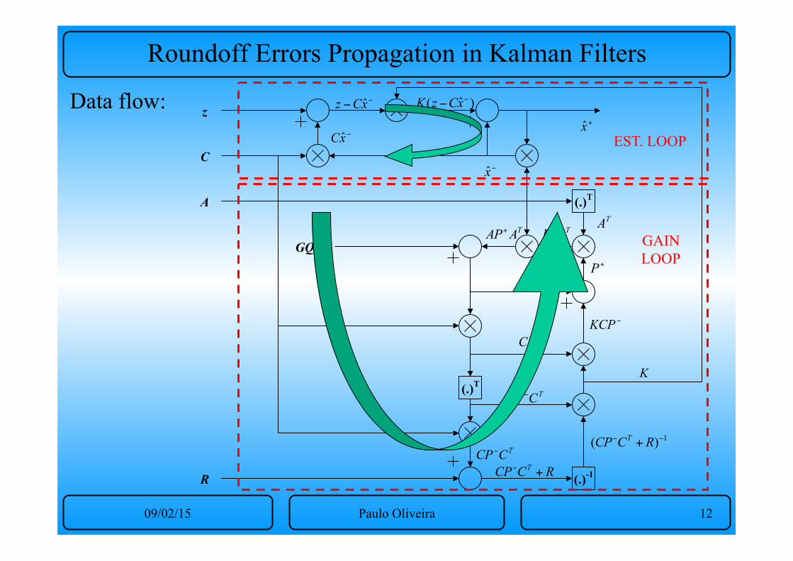
Roundoff Errors Propagation in Kalman Filters
Data flow:
(.)T
(.)T
(.)-1
z
C
A
GQGT
R
−− xCz ˆ )ˆ( −− xCzK
K
−x
−xC ˆ
TA
−P
+P
TAP+TAAP+
−CP
−KCP
TCP−
TCCP−
RCCP T +−
1)( −− + RCCP T
EST. LOOP
GAIN LOOP
+x
09/02/15 Paulo Oliveira 12
Roundoff Errors Propagation in Kalman Filters
Data flow:
(.)T
(.)T
(.)-1
z
C
A
GQGT
R
−− xCz ˆ )ˆ( −− xCzK
K
−x
−xC ˆ
TA
−P
+P
TAP+TAAP+
−CP
−KCP
TCP−
TCCP−
RCCP T +−
1)( −− + RCCP T
EST. LOOP
GAIN LOOP
+x
09/02/15 Paulo Oliveira 13
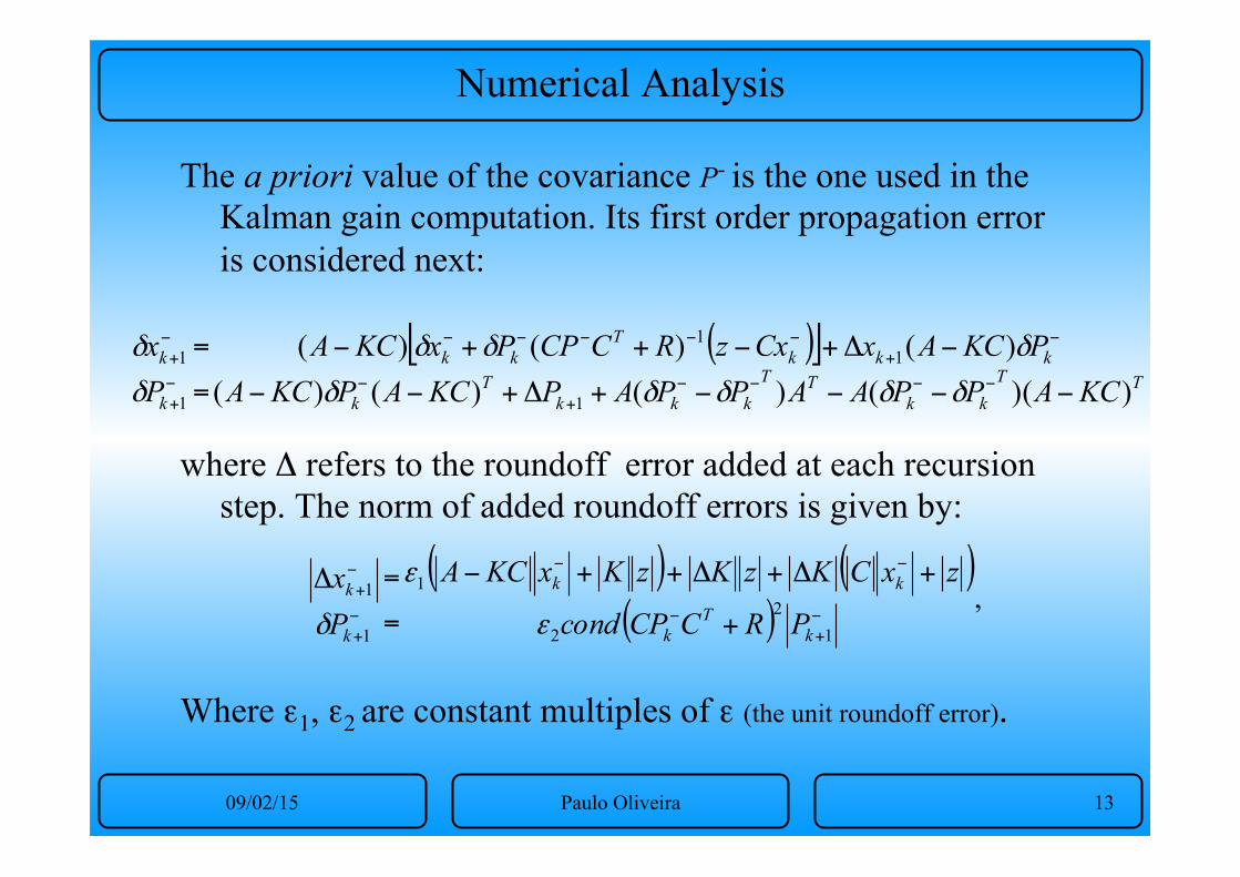
Numerical Analysis
The a priori value of the covariance P- is the one used in the Kalman gain computation. Its first order propagation error is considered next:
where Δ refers to the roundoff error added at each recursion
step. The norm of added roundoff errors is given by: Where ε1, ε2 are constant multiples of ε (the unit roundoff error).
( )[ ],
))(()()()()()()(
1
11
1
1TT
kkTT
kkkT
k
kkkT
kk
k
k
KCAPPAAPPAPKCAPKCAPKCAxCxzRCCPPxKCA
Px
−−−−+Δ+−−
−Δ+−++−
=
=−−−−
+−
−+
−−−−−
−+
−+
δδδδδ
δδδ
δ
δ
( ) ( )( ) ,
12
2
1
1
1−+
−
−−
−+
−+
+
+Δ+Δ++−
=
=Δ
kT
k
kk
k
k
PRCCPcond
zxCKzKzKxKCA
Px
ε
ε
δ
09/02/15 Paulo Oliveira 14
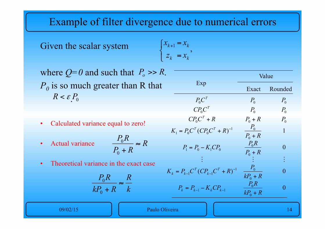
Example of filter divergence due to numerical errors
Given the scalar system where Q=0 and such that . P0 is so much greater than R that . • Calculated variance equal to zero!
• Actual variance
• Theoretical variance in the exact case
,1
⎩⎨⎧
=
=+
k
k
k
k
xx
zx
RPo >>
0PR ε<
Exp Value
Exact Rounded
0
0)(
0
1)(
0
011
0
0111
0
00101
0
01001
000
000
000
RkPRPCPKPP
RkPPRCCPCPK
RPRPCPKPP
RPPRCCPCPK
PRPRCCPPPCCPPPCP
kkkk
Tk
Tkk
TT
T
T
T
+−=
++=
+−=
++=
++
−−
−−−
−
!!!
RRPRP
≈+0
0
kR
RkPRP
≈+0
0

09/02/15 Paulo Oliveira 15
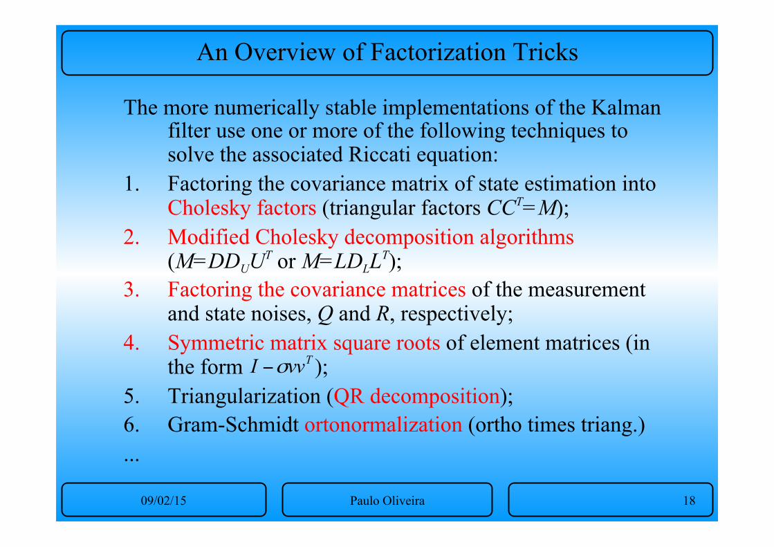
An Overview of Factorization Tricks
The more numerically stable implementations of the Kalman filter use one or more of the following techniques to solve the associated Riccati equation:
1. Factoring the covariance matrix of state estimation into Cholesky factors (triangular factors CCT=M);
2. Modified Cholesky decomposition algorithms (M=DDUUT or M=LDLLT);
3. Factoring the covariance matrices of the measurement and state noises, Q and R, respectively;
4. Symmetric matrix square roots of element matrices (in the form );
5. Triangularization (QR decomposition); 6. Gram-Schmidt ortonormalization (ortho times triang.) ...
TvvI σ−
09/02/15 Paulo Oliveira 16
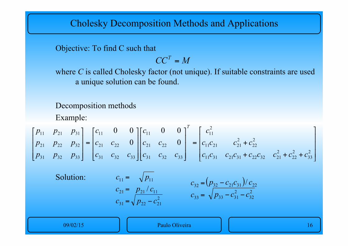
Cholesky Decomposition Methods and Applications
Objective: To find C such that where C is called Cholesky factor (not unique). If suitable constraints are used
a unique solution can be found. Decomposition methods Example: Solution:
MCCT =
⎥⎥⎥
⎦
⎤
⎢⎢⎢
⎣
⎡
+++
+=
⎥⎥⎥
⎦
⎤
⎢⎢⎢
⎣
⎡
⎥⎥⎥
⎦
⎤
⎢⎢⎢
⎣
⎡
=
⎥⎥⎥
⎦
⎤
⎢⎢⎢
⎣
⎡
233
222
221322231213111
222
2212111
211
333231
2221
11
333231
2221
11
333231
322221
312111
000
000
ccccccccccccc
c
ccccc
c
ccccc
c
ppppppppp T
22122
1121
11
31
21
11
/cpcpp
ccc
−=
=
= ( )232
23133
22312132
33
32 /ccpcccp
cc
−−
−
=
=
09/02/15 Paulo Oliveira 17
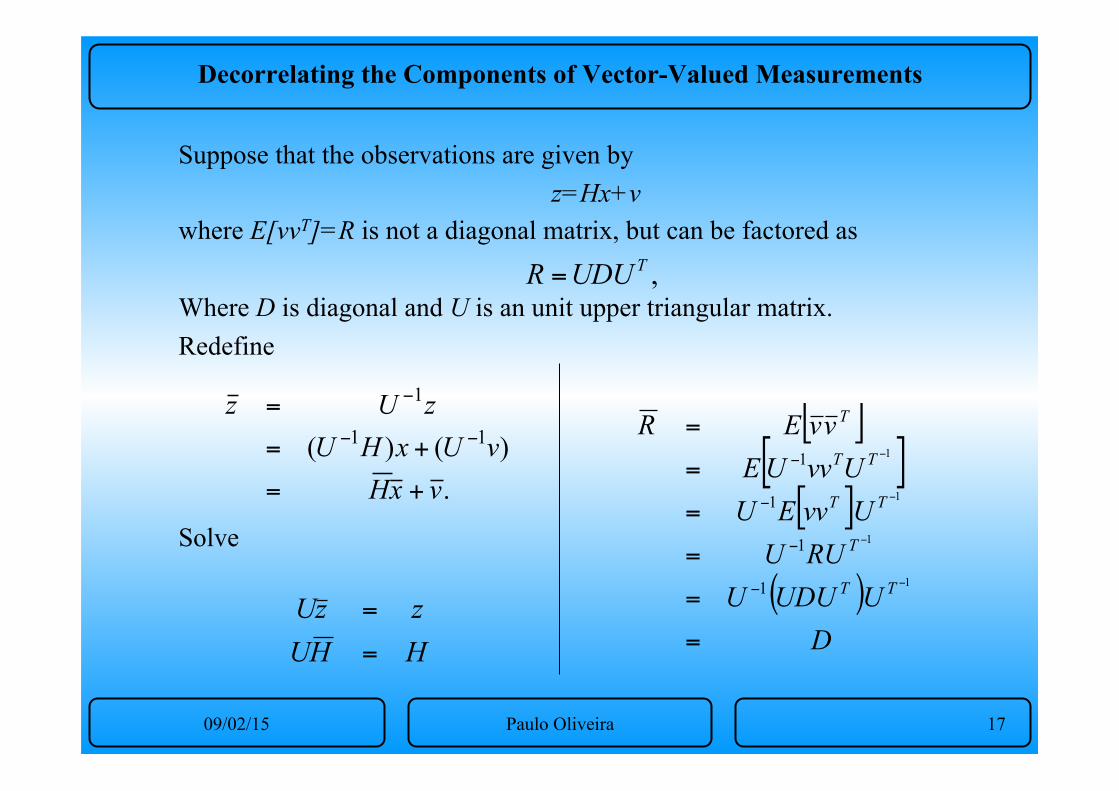
Decorrelating the Components of Vector-Valued Measurements
Suppose that the observations are given by z=Hx+v
where E[vvT]=R is not a diagonal matrix, but can be factored as Where D is diagonal and U is an unit upper triangular matrix. Redefine Solve
,TUDUR =
.)()( 11
1
vxHvUxHU
zUz
+=
+=
=−−
−
[ ][ ][ ]
( )D
UUDUURUU
UvvEUUvvUEvvER
TT
T
TT
TT
T
=
=
=
=
=
=
−
−
−
−
−
−
−
−
1
1
1
1
1
1
1
1
HHUzzU
=
=
09/02/15 Paulo Oliveira 18
An Overview of Factorization Tricks
The more numerically stable implementations of the Kalman filter use one or more of the following techniques to solve the associated Riccati equation:
1. Factoring the covariance matrix of state estimation into Cholesky factors (triangular factors CCT=M);
2. Modified Cholesky decomposition algorithms (M=DDUUT or M=LDLLT);
3. Factoring the covariance matrices of the measurement and state noises, Q and R, respectively;
4. Symmetric matrix square roots of element matrices (in the form );
5. Triangularization (QR decomposition); 6. Gram-Schmidt ortonormalization (ortho times triang.) ...
TvvI σ−
09/02/15 Paulo Oliveira 19
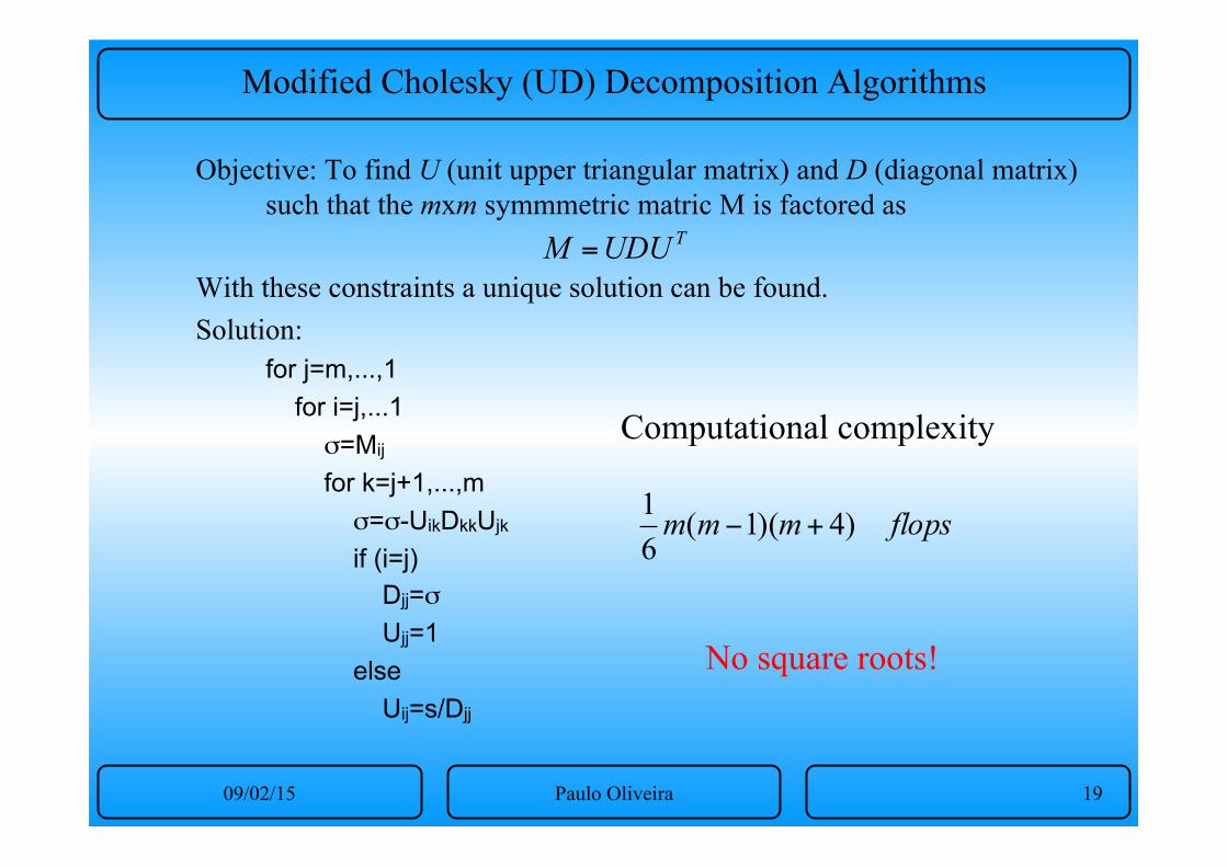
Modified Cholesky (UD) Decomposition Algorithms
Objective: To find U (unit upper triangular matrix) and D (diagonal matrix) such that the mxm symmmetric matric M is factored as
With these constraints a unique solution can be found. Solution:
for j=m,...,1 for i=j,...1
σ=Mij
for k=j+1,...,m σ=σ-UikDkkUjk
if (i=j) Djj=σ Ujj=1 else Uij=s/Djj
TUDUM =
Computational complexity
flopsmmm )4)(1(61
+−
No square roots!
09/02/15 Paulo Oliveira 20
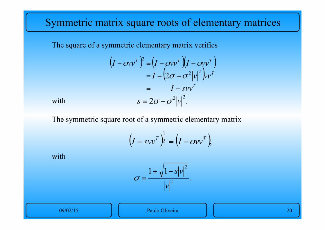
Symmetric matrix square roots of elementary matrices
The square of a symmetric elementary matrix verifies with The symmetric square root of a symmetric elementary matrix with
( ) ( )( )( )
T
T
TTT
svvIvvvIvvIvvIvvI
−
−−
−−
=
=
=−22
2
2 σσ
σσσ
.2 22 vs σσ −=
.112
2
v
vs−+=σ
( ) ( ),21
TT vvIsvvI σ−=−
09/02/15 Paulo Oliveira 21
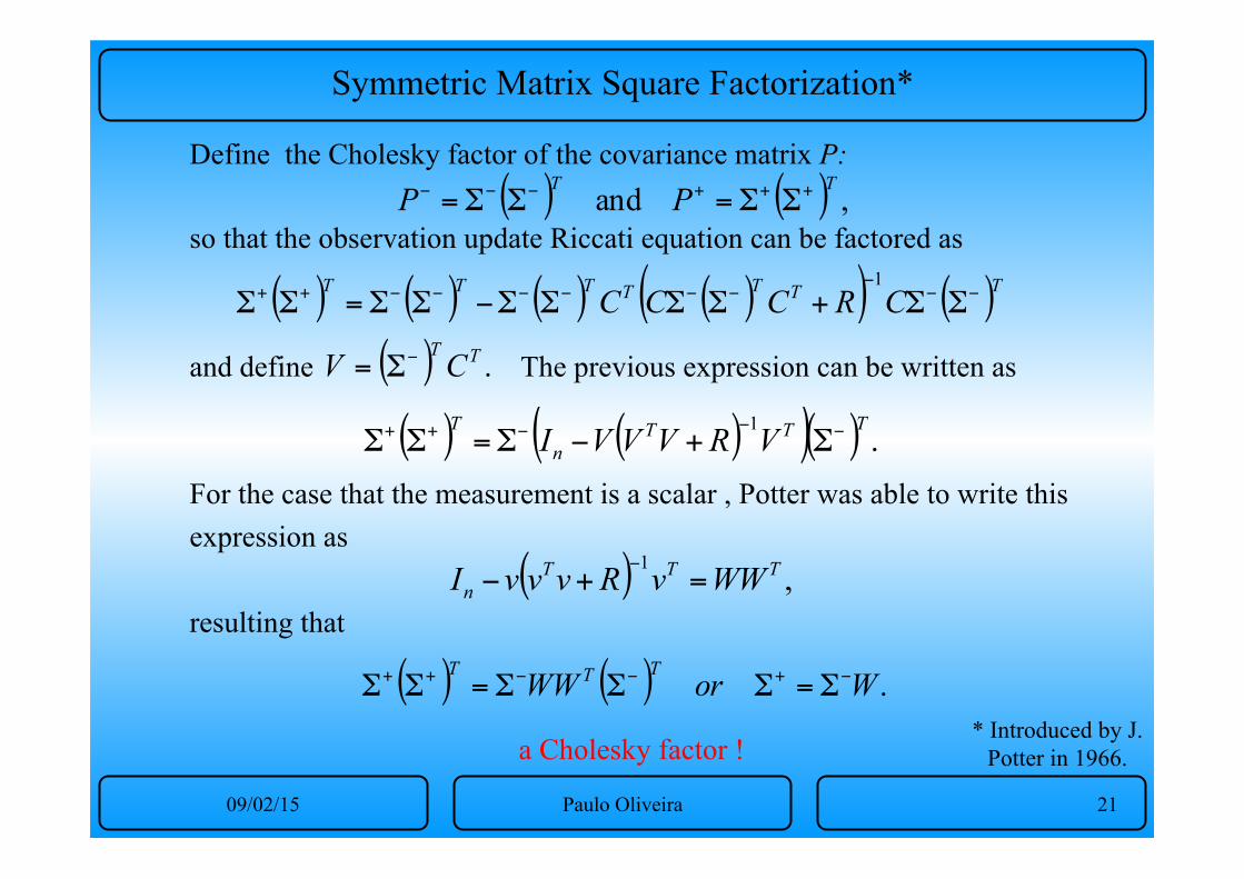
Symmetric Matrix Square Factorization*
* Introduced by J. Potter in 1966.
Define the Cholesky factor of the covariance matrix P: so that the observation update Riccati equation can be factored as and define The previous expression can be written as For the case that the measurement is a scalar , Potter was able to write this expression as resulting that
a Cholesky factor !
( ) ( ) ,and TT PP +++−−− ΣΣ=ΣΣ=
( ) ( ) ( ) ( )( ) ( )TTTTTTT CRCCC −−−
−−−−−−++ ΣΣ+ΣΣΣΣ−ΣΣ=ΣΣ1
( ) .TT CV −Σ=
( ) ( )( )( ) .1 TTTn
T VRVVVI −−−++ Σ+−Σ=ΣΣ
( ) ,1 TTTn WWvRvvvI =+−
−
( ) ( ) .WorWW TTT −+−−++ Σ=ΣΣΣ=ΣΣ
09/02/15 Paulo Oliveira 22
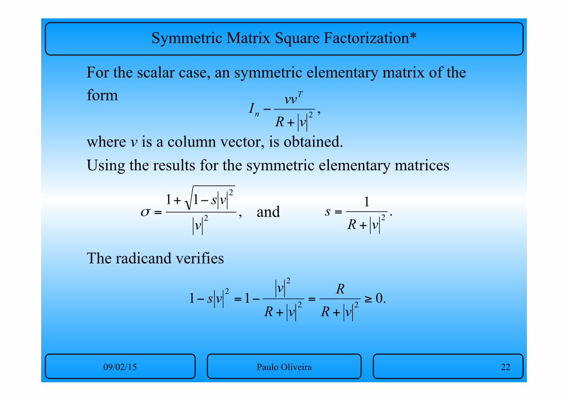
Symmetric Matrix Square Factorization*
For the scalar case, an symmetric elementary matrix of the form where v is a column vector, is obtained. Using the results for the symmetric elementary matrices and The radicand verifies
,2vRvvIT
n+
−
,112
2
v
vs−+=σ .1
2vRs
+=
.011 22
22
≥+
=+
−=−vRR
vRv
vs
09/02/15 Paulo Oliveira 23
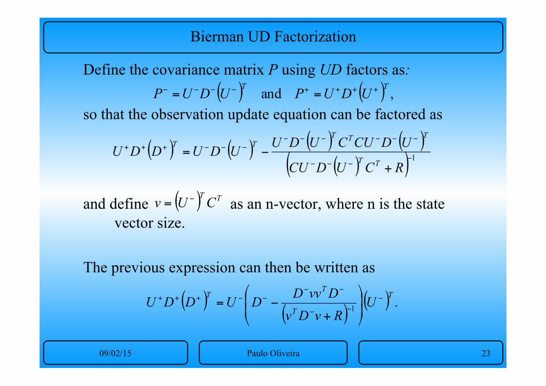
Bierman UD Factorization
Define the covariance matrix P using UD factors as: so that the observation update equation can be factored as and define as an n-vector, where n is the state
vector size. The previous expression can then be written as
( ) ( ) ,and TT UDUPUDUP ++++−−−− ==
( ) ( ) ( ) ( )( )( ) 1−−−−
−−−−−−−−−+++
+−=
RCUDCU
UDCUCUDUUDUDDUTT
TTTTT
( ) TT CUv −=
( )( )
( ) .1
T
T
TT U
RvDvDvvDDUDDU −
−−
−−−−+++
⎟⎟⎠
⎞⎜⎜⎝
⎛
+−=
09/02/15 Paulo Oliveira 24
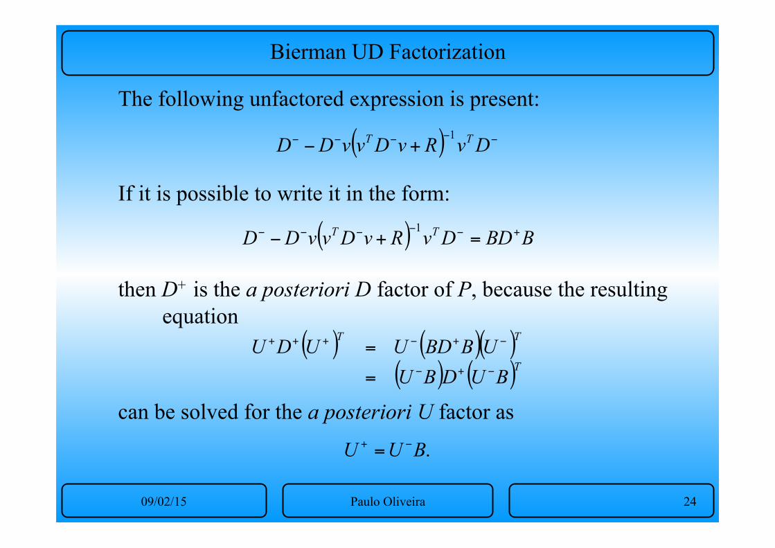
Bierman UD Factorization
The following unfactored expression is present: If it is possible to write it in the form: then D+ is the a posteriori D factor of P, because the resulting
equation can be solved for the a posteriori U factor as
.BUU −+ =
( ) ( )( )( ) ( )T
TT
BUDBUUBBDUUDU−+−
−+−+++
=
=
( ) −−−−− +− DvRvDvvDD TT 1
( ) BBDDvRvDvvDD TT +−−−−− =+−1
09/02/15 Paulo Oliveira 25
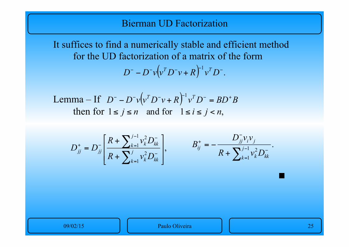
Bierman UD Factorization
It suffices to find a numerically stable and efficient method for the UD factorization of a matrix of the form
Lemma – If
then for
,12
1
12
⎥⎥
⎦
⎤
⎢⎢
⎣
⎡
+
+=
∑∑
=
−
−
=
−−+
j
k kkk
j
k kkkjjjj
DvR
DvRDD
( ) .1 −−−−− +− DvRvDvvDD TT
( ) BBDDvRvDvvDD TT +−−−−− =+−1
,1forand1 njinj <≤≤≤≤
.1
12∑
−
=
−
−+
+−= j
k kkk
jijjij
DvR
vvDB
09/02/15 Paulo Oliveira 26
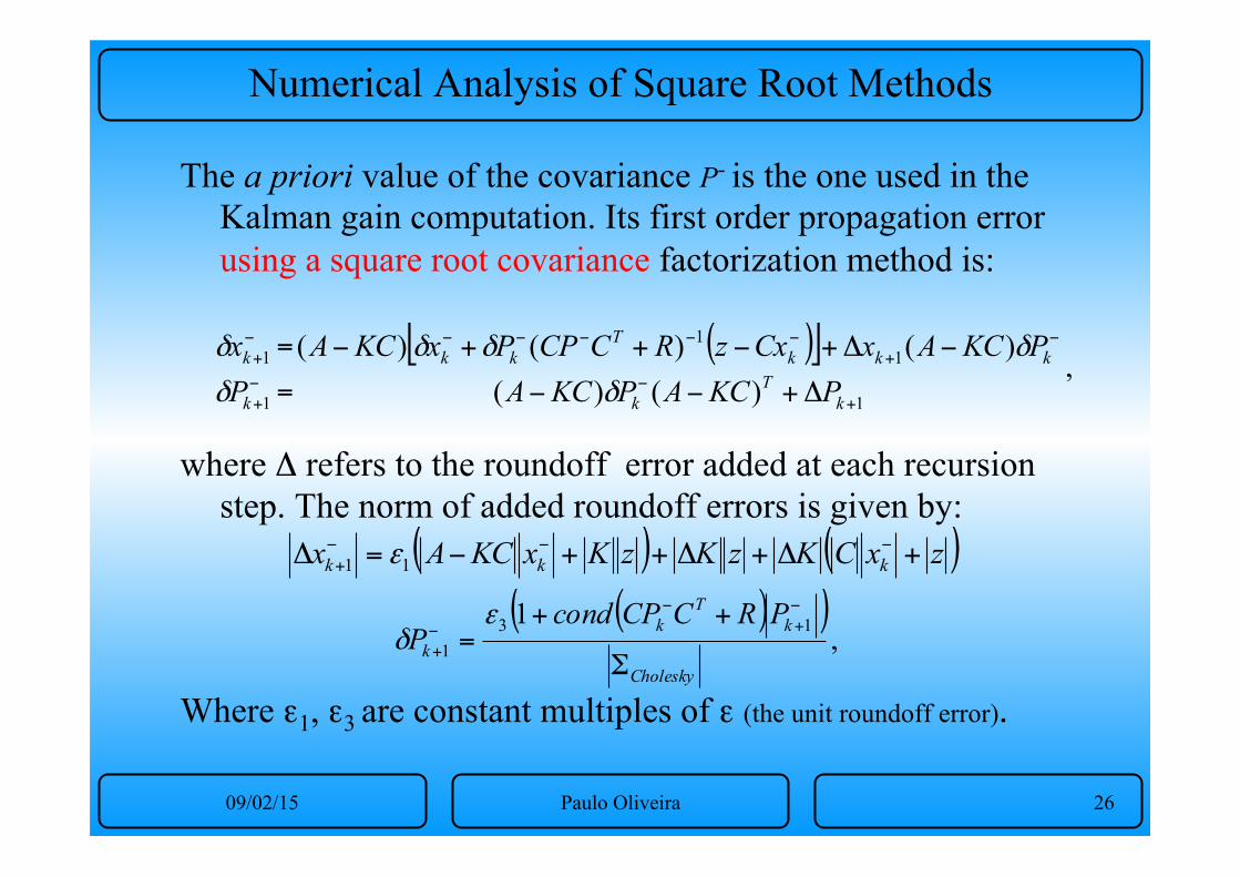
Numerical Analysis of Square Root Methods
The a priori value of the covariance P- is the one used in the Kalman gain computation. Its first order propagation error using a square root covariance factorization method is:
where Δ refers to the roundoff error added at each recursion
step. The norm of added roundoff errors is given by: Where ε1, ε3 are constant multiples of ε (the unit roundoff error).
( )[ ],
)()()()()(
1
11
1
1
+−
−+
−−−−−
−+
−+
Δ+−−
−Δ+−++−
=
=
kT
k
kkkT
kk
k
k
PKCAPKCAPKCAxCxzRCCPPxKCA
Px
δ
δδδ
δ
δ
( )( ),
1 131
Cholesky
kT
kk
PRCCPcondP
Σ
++=
−+
−
−+
εδ
( ) ( )zxCKzKzKxKCAx kkk +Δ+Δ++−=Δ −−−+ 11 ε
09/02/15 Paulo Oliveira 27
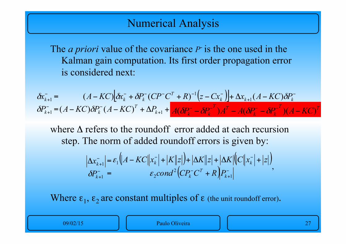
Numerical Analysis
The a priori value of the covariance P- is the one used in the Kalman gain computation. Its first order propagation error is considered next:
where Δ refers to the roundoff error added at each recursion
step. The norm of added roundoff errors is given by: Where ε1, ε2 are constant multiples of ε (the unit roundoff error).
( )[ ],
))(()()()()()()(
1
11
1
1TT
kkTT
kkkT
k
kkkT
kk
k
k
KCAPPAAPPAPKCAPKCAPKCAxCxzRCCPPxKCA
Px
−−−−+Δ+−−
−Δ+−++−
=
=−−−−
+−
−+
−−−−−
−+
−+
δδδδδ
δδδ
δ
δ
( ) ( )( ) ,
12
2
1
1
1−+
−
−−
−+
−+
+
+Δ+Δ++−
=
=Δ
kT
k
kk
k
k
PRCCPcondzxCKzKzKxKCA
Px
ε
ε
δ
TTkk
TTkk KCAPPAAPPA ))(()( −−−− −−−− δδδδ
09/02/15 Paulo Oliveira 28
• Kalman Filtering: Theory and Practice - M. Grewal and A. Andrews, Prentice Hall, 1993;
• Applied Optimal Estimation, A. Gelb, MIT Press, 1974;
• Optimal Filtering, B. Anderson and J. Moore, Prentice Hall, 1979.
• Factorization Methods for Discrete Sequential Estimation, G. J. Bierman, New York: Academic Press, 1977.
Bibliography

1!
H∞ Filtering and Smoothing"
PAULO OLIVEIRA!!
DEEC/IST and ISR!!
Last Revised: November 10, 2007!Ref. No. NLO#1!
2!
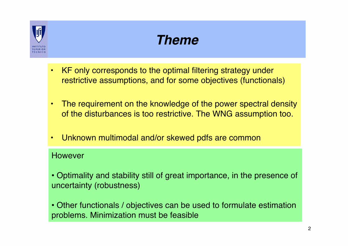
Theme"
• KF only corresponds to the optimal filtering strategy under restrictive assumptions, and for some objectives (functionals)!
• The requirement on the knowledge of the power spectral density of the disturbances is too restrictive. The WNG assumption too.!
• Unknown multimodal and/or skewed pdfs are common!
However!
• Optimality and stability still of great importance, in the presence of uncertainty (robustness)!
• Other functionals / objectives can be used to formulate estimation problems. Minimization must be feasible!
3!
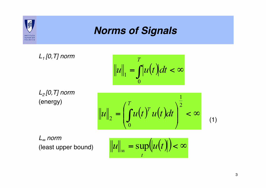
Norms of Signals"
L1 [0,T] norm !!!!L2 [0,T] norm !(energy) !!! ! ! ! ! ! ! ! ! !(1)!
!L∞ norm !(least upper bound)!
( ) ∞<= ∫T
dttuu0
1
( ) ( ) ∞<⎟⎟⎠
⎞⎜⎜⎝
⎛= ∫
21
02
TT dttutuu
( )( ) ∞<=∞
tuutsup
4!
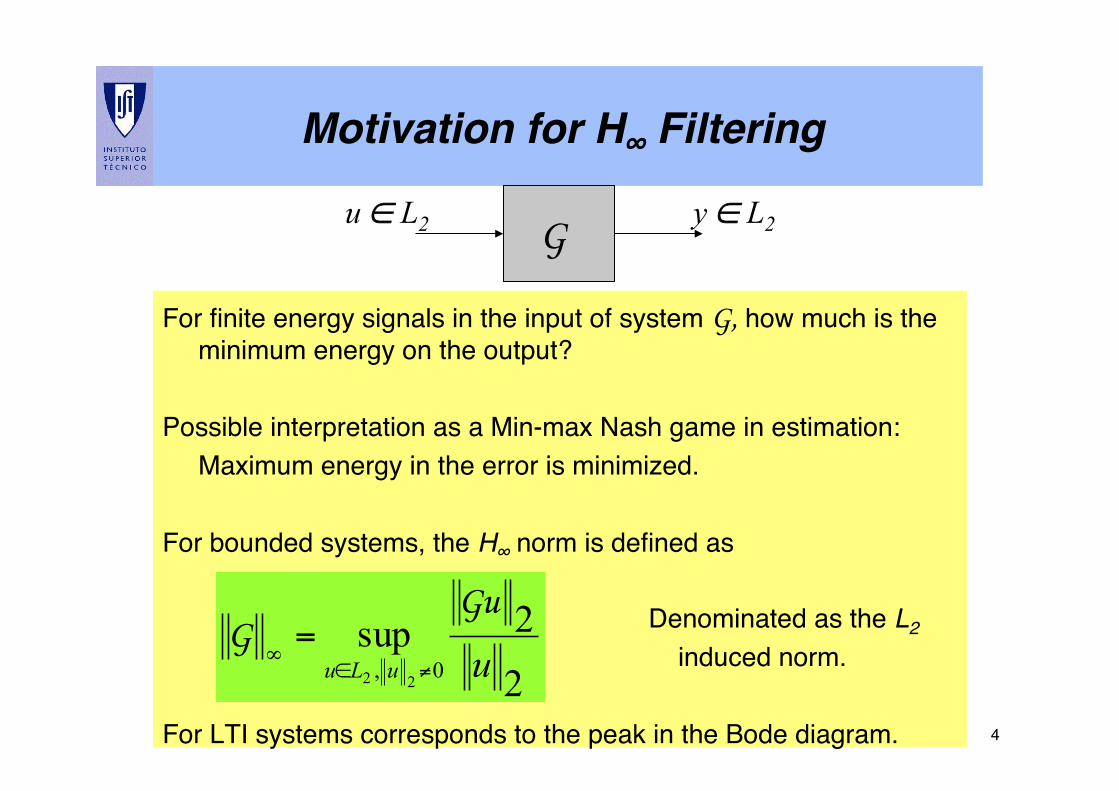
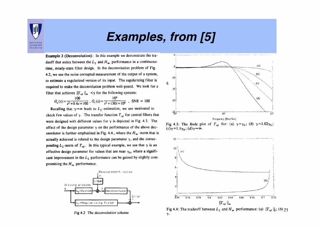
Motivation for H∞ Filtering "
For finite energy signals in the input of system G, how much is the minimum energy on the output? !
!Possible interpretation as a Min-max Nash game in estimation:!!Maximum energy in the error is minimized.!! ! ! ! !!
For bounded systems, the H∞ norm is defined as!!! ! ! ! ! ! ! Denominated as the L2 !! ! ! ! ! ! ! induced norm.!
!For LTI systems corresponds to the peak in the Bode diagram.!
G u ∈ L2 y ∈ L2
2
2sup0, 22 uuLu
GuG
≠∈∞=
5!
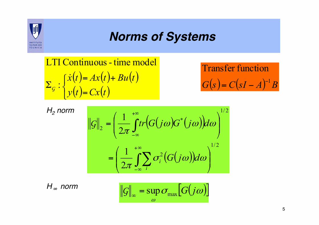
Norms of Systems"
H2 norm!!!!!!!H ∞ norm!!
( )( )
( )( )
( )⎩⎨⎧ +
=
=Σ
tButCxtAx
tytx!
:
model time-Continuous LTI
G ( ) ( ) BAsICsG 1
functionTransfer −−=
( ) ( )( )
( )( )2/1
2
2/1
*2
21
21
⎟⎟⎠
⎞⎜⎜⎝
⎛=
⎟⎟⎠
⎞⎜⎜⎝
⎛=
∫∑
∫∞+
∞−
+∞
∞−
ωωσπ
ωωωπ
djG
djGjGtr
ii
G
( )[ ]ωσω
jGmaxsup=∞
G
6!
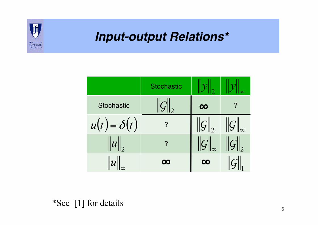
Input-output Relations*"
Stochastic!
Stochastic! ?!
?!
?!
( ) ( )ttu δ=
2u
2G
2y
∞y
2G
∞G
∞G
2G
*See [1] for details
∞u
1G∞"∞"
∞"
7!
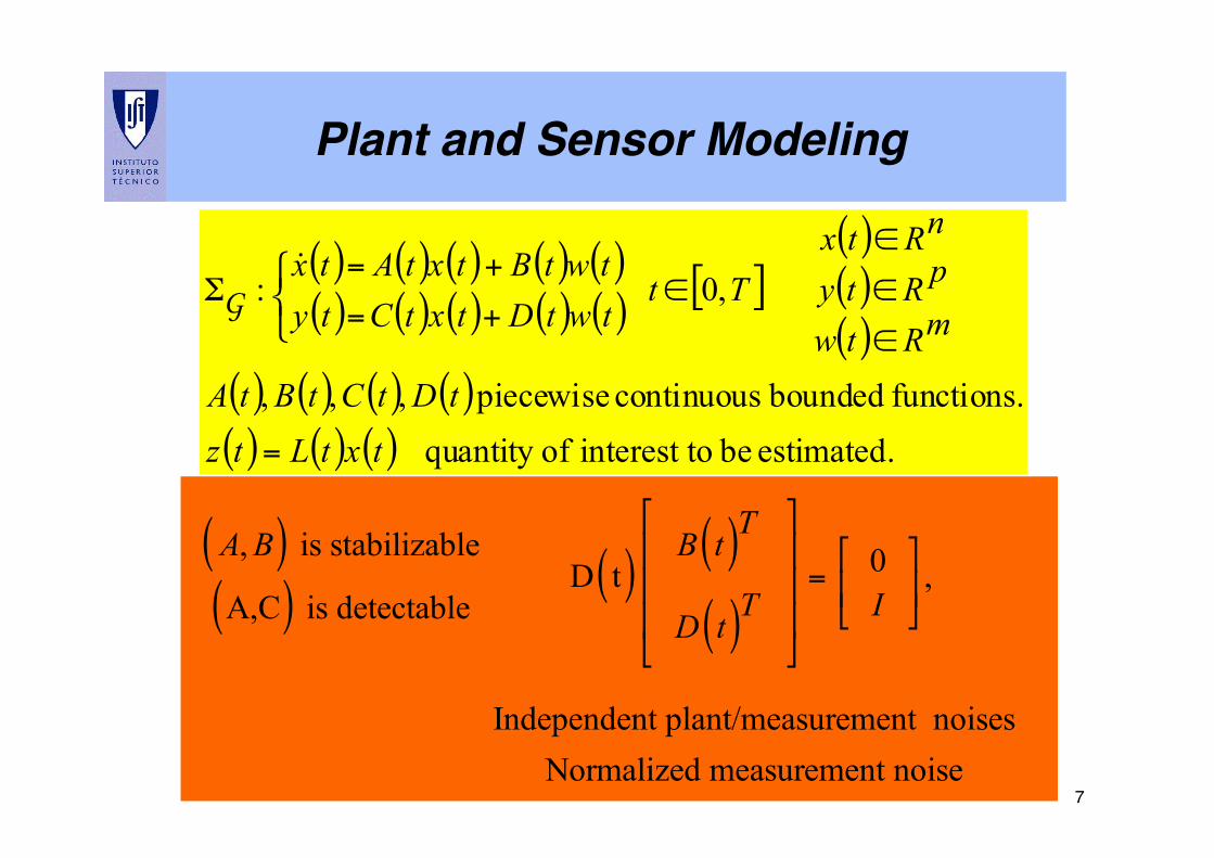
Plant and Sensor Modeling "
( )( )
( ) ( )( ) ( )
( ) ( )( ) ( ) [ ]
( )( )( )
( ) ( ) ( ) ( )( ) ( ) ( ) estimated. be ointerest t ofquantity
functions. bounded continuous piecewise ,,,
,0:
txtLtztDtCtBtA
mRtw
pRty
nRtxTt
twtDtwtB
txtCtxtA
tytx
=
∈
∈
∈
∈+
+
=
=Σ
⎩⎨⎧ !
G
Assume that !!!
A, B( ) is stabilizable
A,C( ) is detectableD t( )
B t( )T
D t( )T
!
"
###
$
%
&&&= 0
I!
"#
$
%& ,
Independent plant/measurement noisesNormalized measurement noise
8!
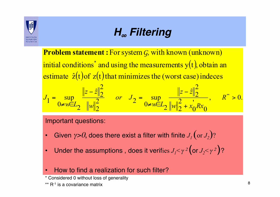
H∞ Filtering"
( )( ) ( )
.0,
0'0
22
22ˆ
20sup22
2
22ˆ
20sup1
**
indeces case)(worst theminimizes that tz of tz estimatean obtain ,ty tsmeasuremen theusing and conditions initial
(unknown)known with systemFor *
>+
−
∈≠=
−
∈≠= R
Rxxw
zz
LwJor
w
zz
LwJ
G, :statement Problem
Important questions:!
• Given γ>0, does there exist a filter with finite J1 (or J2)?
• Under the assumptions , does it verifies J1<γ 2 (or J2<γ 2 )?!
• How to find a realization for such filter?!* Considered 0 without loss of generality!** R-1 is a covariance matrix!
!
9!
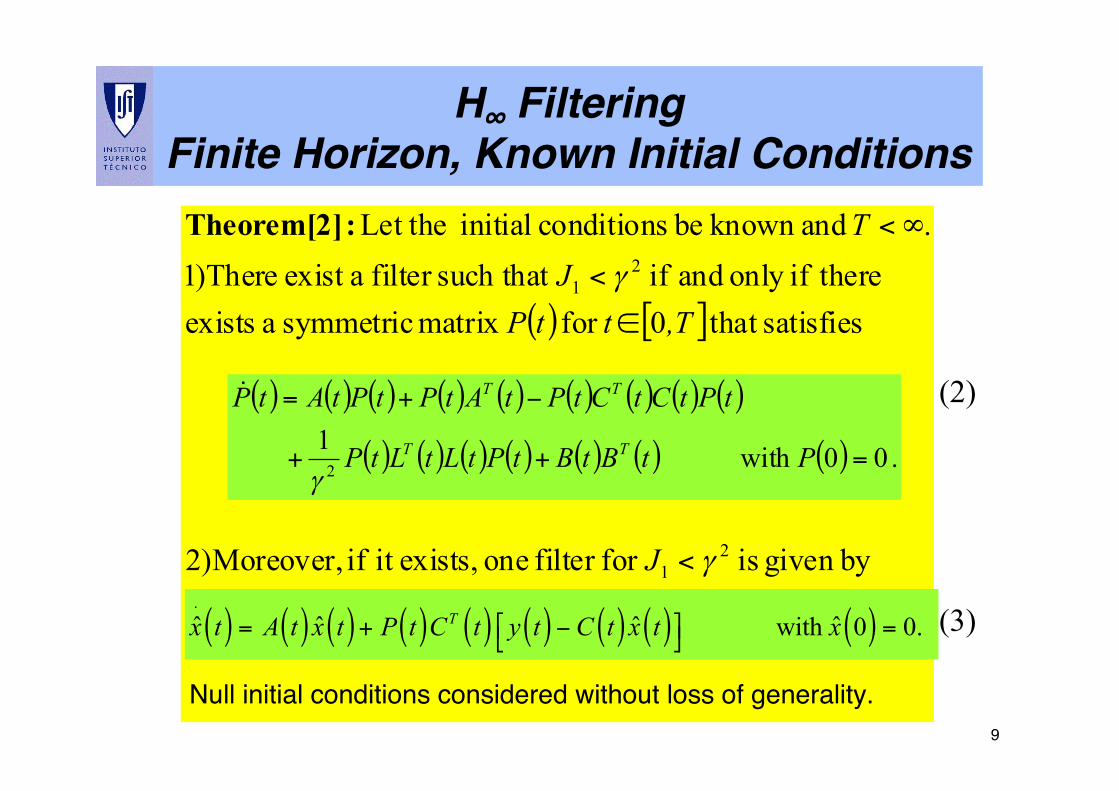
H∞ FilteringFinite Horizon, Known Initial Conditions"
( ) [ ]
bygiven is for filter one exists,it if Moreover,)2
satisfies that 0for matrix symmetric a exists thereifonly and if such that filter aexist There)1
. andknown be conditions initial Let the
21
21
γ
γ
<
∈
<
∞<
J
,TttPJ
T :Theorem[2]
( ) ( ) ( ) ( ) ( ) ( ) ( ) ( ) ( )
( ) ( ) ( ) ( ) ( ) ( ) ( ) . 00with 12 =++
−+=
PtBtBtPtLtLtP
tPtCtCtPtAtPtPtAtP
TT
TT
γ
!
x.
t( ) = A t( ) x t( ) + P t( )CT t( ) y t( ) − C t( ) x t( )"# $% with x 0( ) = 0.
(2) (3)
Null initial conditions considered without loss of generality.!
10!
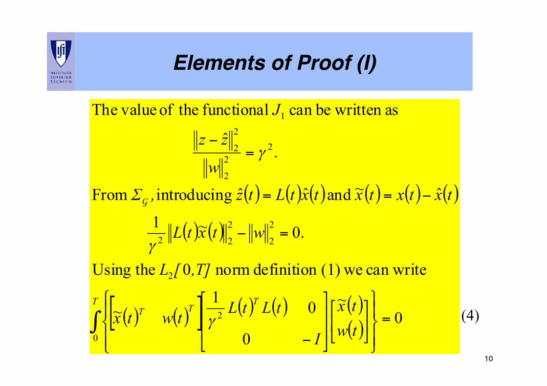
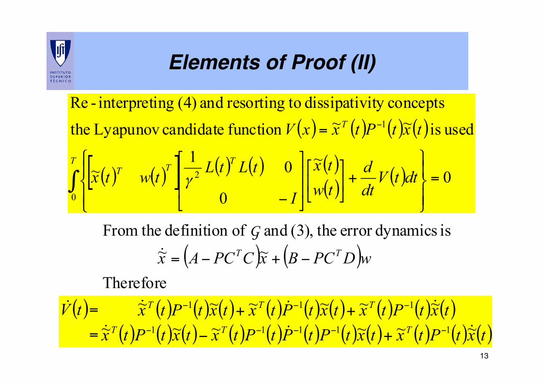
Elements of Proof (I)"
( ) ( ) ( ) ( ) ( ) ( )
( ) ( )
( ) ( )[ ] ( ) ( ) ( )( )∫ =
⎪⎭
⎪⎬
⎫
⎪⎩
⎪⎨
⎧
⎥⎦
⎤⎢⎣
⎡⎥⎥
⎦
⎤
⎢⎢
⎣
⎡
−
=−
−==
=−
T TTT
twtx
I
tLtLtwtx
,T][L
wtxtL
txtxtxtxtLtzΣ
w
zz
J
0
2
2
2
2
2
22
22
2
2
2
1
0~
0
01~
can write we(1) definition norm 0 theUsing
.0~1
ˆ~ and ˆˆ gintroducin From
.ˆ
as written becan functional theof valueThe
γ
γ
γ
,G
(4)
11!
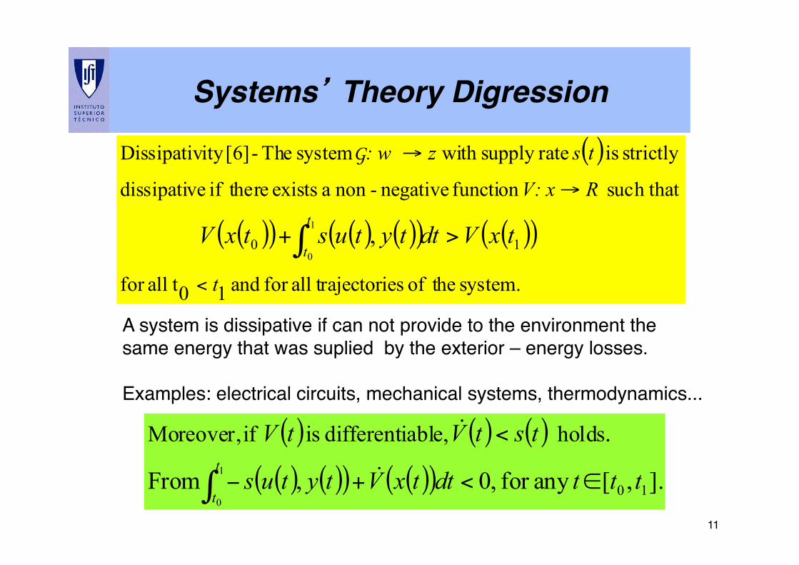
Systems’ Theory Digression"
A system is dissipative if can not provide to the environment the !same energy that was suplied by the exterior – energy losses.!!Examples: electrical circuits, mechanical systems, thermodynamics...!
( )
( )( ) ( ) ( )( ) ( )( )
system. theof ies trajectorallfor and 10 tallfor
such that function negative-non a exists thereif edissipativ
strictly is ratesupply with system The - [6]ity Dissipativ
101
0
,
t
RV: x
tsz: w
txVdttytustxVt
t
<
→
→
>+ ∫
G
( ) ( ) ( )
( ) ( )( ) ( )( ) ].,[any for ,0, From
.
101
0
holds e,iabldifferent is if Moreover,
tttdttxVtytus
tstVtVt
t∈<+−
<
∫ !
!
12!
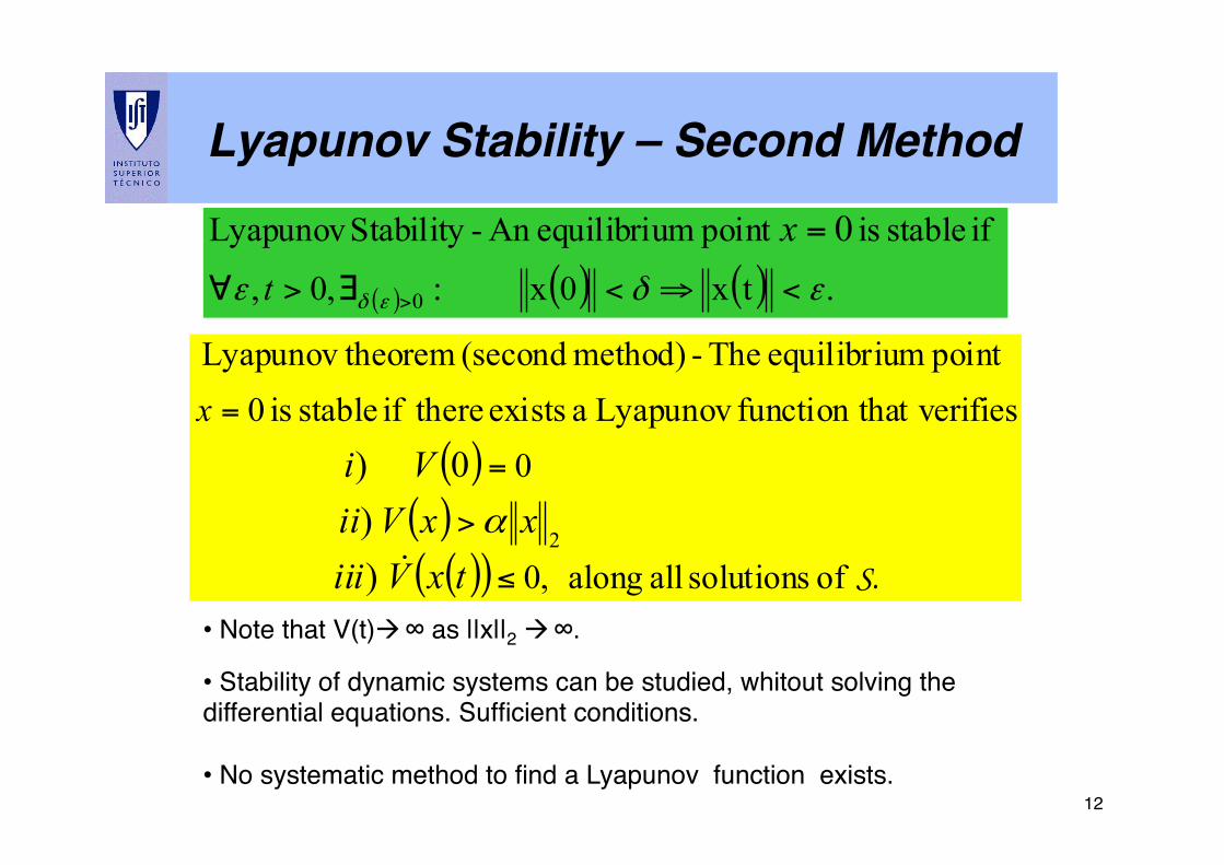
Lyapunov Stability – Second Method"
• Note that V(t)à ∞ as ||x||2 à ∞.!
• Stability of dynamic systems can be studied, whitout solving the differential equations. Sufficient conditions.!
• No systematic method to find a Lyapunov function exists.!
( )( )( )( ) S. of solutions all along ,0
0eshat verififunction t Lyapunov a exists thereif stable is 0
point mequilibriu The - method) (second theoremLyapunov
2
0
)))
≤
>
=
=
txVxxV
V
iiiiii
x
!α
( ) ( ) ( ) .tx0x:,0,
if stable is point mequilibriuAn -Stability Lyapunov
0
0εδε εδ <⇒<∃>∀ >
=
t
x
13!
Elements of Proof (II)"
( ) ( ) ( ) ( )
( ) ( )[ ] ( ) ( ) ( )( )
( )∫ =⎪⎭
⎪⎬
⎫
⎪⎩
⎪⎨
⎧+⎥⎦
⎤⎢⎣
⎡⎥⎥
⎦
⎤
⎢⎢
⎣
⎡
−
= −
T TTT
T
dttVdtd
twtx
I
tLtLtwtx
txtPtxxV
0
2
1
0~
0
01~
used is ~~function candidate Lyapunov the conceptsity dissipativ toresorting and (4) nginterpreti-Re
γ
( ) ( )Therefore
~~is dynamicserror the(3), and of definition theFrom
wDPCBxCPCAx TT −+−=!G
( ) ( ) ( ) ( ) ( ) ( ) ( ) ( ) ( ) ( )( ) ( ) ( ) ( ) ( ) ( ) ( ) ( ) ( ) ( ) ( )txtPtxtxtPtPtPtxtxtPtx
txtPtxtxtPtxtxtPtxtVTTT
TTT
!!!!!!!
~~~~~~~~~~~~11111
111
−−−−−
−−−
+−
++
=
=
14!
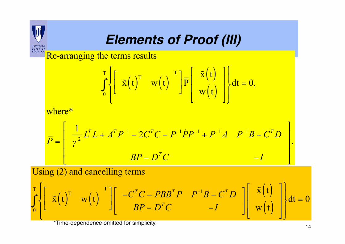
Elements of Proof (III)"
Re-arranging the terms results
!x t( )Tw t( )
T!
"#
$
%&P
!x t( )w t( )
!
"
###
$
%
&&&
'
()
*)
+
,)
-)
dt0
T
∫ = 0,
where*
P =1γ 2
LT L + AT P−1 − 2CTC − P−1 "PP−1 + P−1A P−1B − CT D
BP − DTC − I
!
"
###
$
%
&&&.
Using (2) and cancelling terms
!x t( )Tw t( )
T!
"#
$
%& −CTC − PBBT P P−1B − CT D
BP − DTC − I
!
"##
$
%&&
!x t( )w t( )
!
"
###
$
%
&&&
(
)*
+*
,
-*
.*
dt0
T
∫ = 0
*Time-dependence omitted for simplicity.!
15!
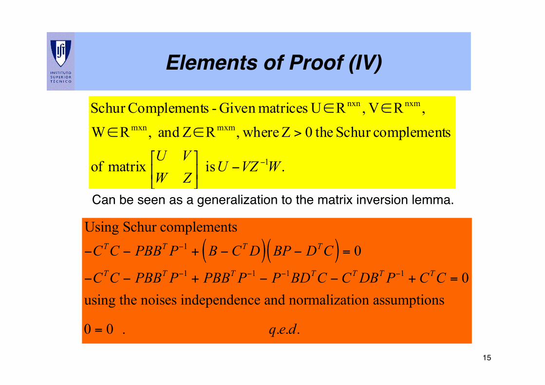
Elements of Proof (IV)"
Using Schur complements
−CTC − PBBT P−1 + B − CT D( ) BP − DTC( ) = 0
−CTC − PBBT P−1 + PBBT P−1 − P−1BDTC − CT DBT P−1 + CTC = 0using the noises independence and normalization assumptions
0 = 0 . q.e.d.
. is matrix of
scomplementSchur the0 Z where,R Zand ,RW,RV ,R UmatricesGiven - sComplementSchur
1
mxmmxn
nxmnxn
WVZUZWVU −−⎥⎦
⎤⎢⎣
⎡
>∈∈
∈∈
Can be seen as a generalization to the matrix inversion lemma. !
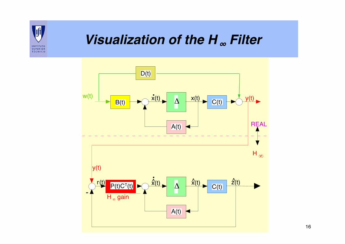
16!
Visualization of the H ∞ Filter"
B(t) w(t) x(t) x(t) Δ y(t) C(t)
A(t)
r (t) x(t) x(t) z(t) C(t)
A(t)
y(t)
-
.
^ ^ ^ .
H ∞ gain
REAL
H ∞
Δ P(t)CT(t)
D(t)
17!
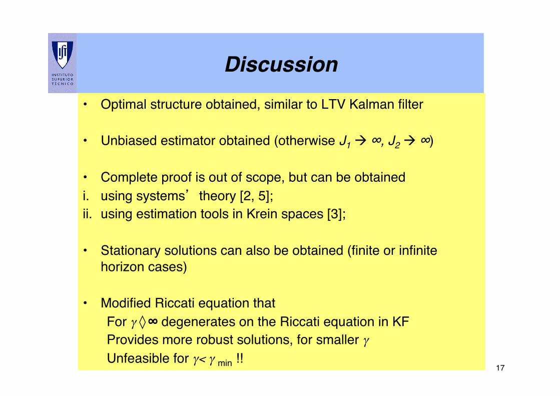
Discussion"• Optimal structure obtained, similar to LTV Kalman filter!
• Unbiased estimator obtained (otherwise J1 à ∞, J2 à ∞)!
• Complete proof is out of scope, but can be obtained !i. using systems’ theory [2, 5]; !ii. using estimation tools in Krein spaces [3]; !!• Stationary solutions can also be obtained (finite or infinite
horizon cases)!
• Modified Riccati equation that!For γ ◊ ∞ degenerates on the Riccati equation in KF Provides more robust solutions, for smaller γ Unfeasible for γ< γ min !!!!
18!
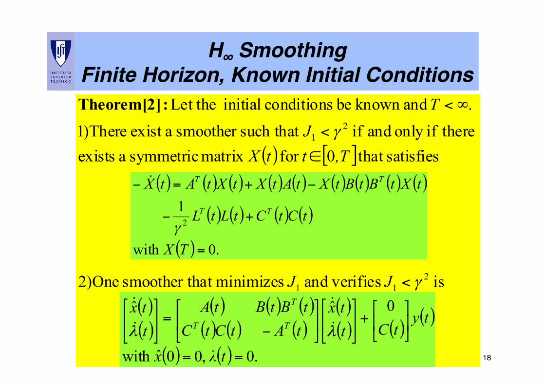
H∞ SmoothingFinite Horizon, Known Initial Conditions"
( ) [ ]
is verifiesand minimizeshat smoother t One)2
satisfies that 0for matrix symmetric a exists thereifonly and if such that smoother aexist There)1
. andknown be conditions initial Let the
211
21
γ
γ
<
∈
<
∞<
JJ
,TttXJ
T :Theorem[2]
( ) ( ) ( ) ( ) ( ) ( ) ( ) ( ) ( )
( ) ( ) ( ) ( )
( ) .0with
12
=
+−
−+=−
TX
tCtCtLtL
tXtBtBtXtAtXtXtAtX
TT
TT
γ
!
( )( )
( ) ( ) ( )( ) ( ) ( )
( )( ) ( )
( )
( ) ( ) .0 ,00ˆwith
0ˆˆ
==
⎥⎦
⎤⎢⎣
⎡+⎥⎦
⎤⎢⎣
⎡⎥⎦
⎤⎢⎣
⎡
−=⎥
⎦
⎤⎢⎣
⎡
tλx
tytCt
txtAtCtCtBtBtA
ttx
TT
T
λλ !
!
!
!
19!
Remarks"
• Proof is omitted, see [2] for details.!
• The H ∞ smoother structure is equal to the H2!!
• Smoothers for all 4 cases are well known.!
• Much more recent results than the H2 solutions!
• Other functionals have already been solved, e.g. mixed H2/H ∞ Also, solutions for nonlinear cases available!
• Now a couples of examples from [5] are included to document some of the results outlined!
20!
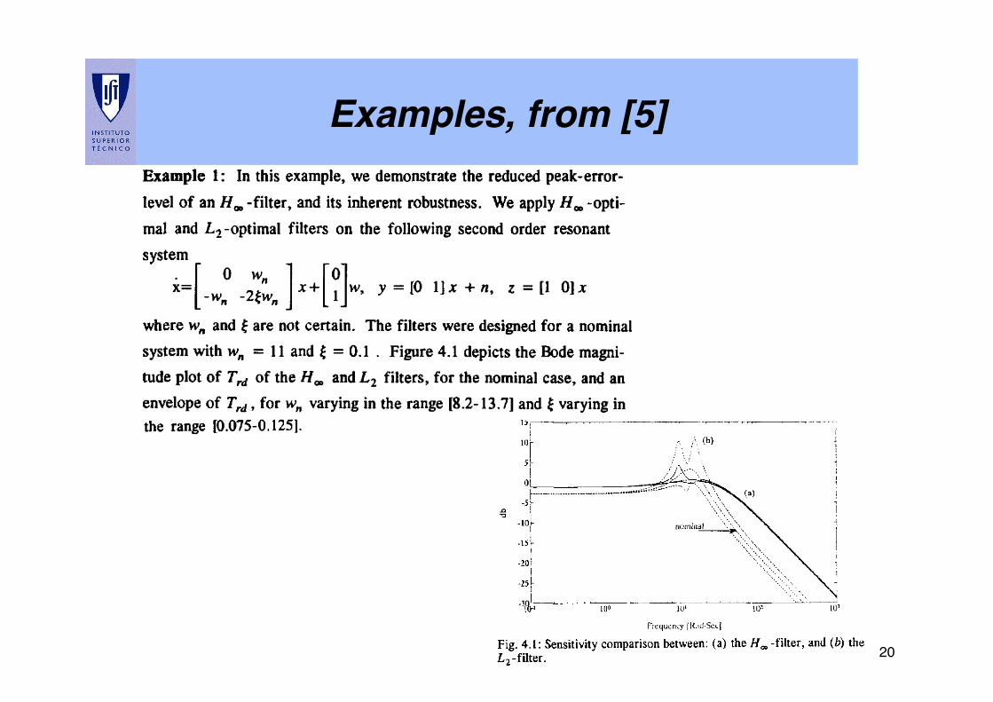
Examples, from [5]"
21!
Examples, from [5]"
22!
References"
[1] J. Doyle, B. Francis, and A. Tannenbaum, Feedback Control Theory, Macmillan Press, 1990 !
[2] K. Nagpal and P. Khargonekar, “Filtering and Smoothing in the H∞ Setting,” IEEE TAC, vol 36, n2, Feb. 1991!
[3] B. Hassibi, A. Sayed, and T, Kailath, “Linear Estimation in Krein Stpaces – Part I Theory,” IEEE TAC, vol 41, n1, Jan. 1996!
[4] C. Scherer, P. Gahinet, and M. Chilali, “Multiobjective Output-feedback Control Via LMI Optimization,” IEEE TAC, vol 42, n7, 1997!
[5] U. Shaked and Y. Theodor, “H∞-Optimal Estimation: A Tutorial,” Proc. CDC, pp. 2278-2286Arizona, USA,1992. !
[6] J. Willems, “Dissipative dynamic systems,” Arch. Rational Mech. Anal, Vol. 45, pp. 321-393, 1971.!

1!
New Methods for State Estimation!
PAULO OLIVEIRA!!
DEEC/IST and ISR!!
Last Revised: December 14, 2007!Ref. No. NLO#2!
2!
Key Challenges in Estimation!
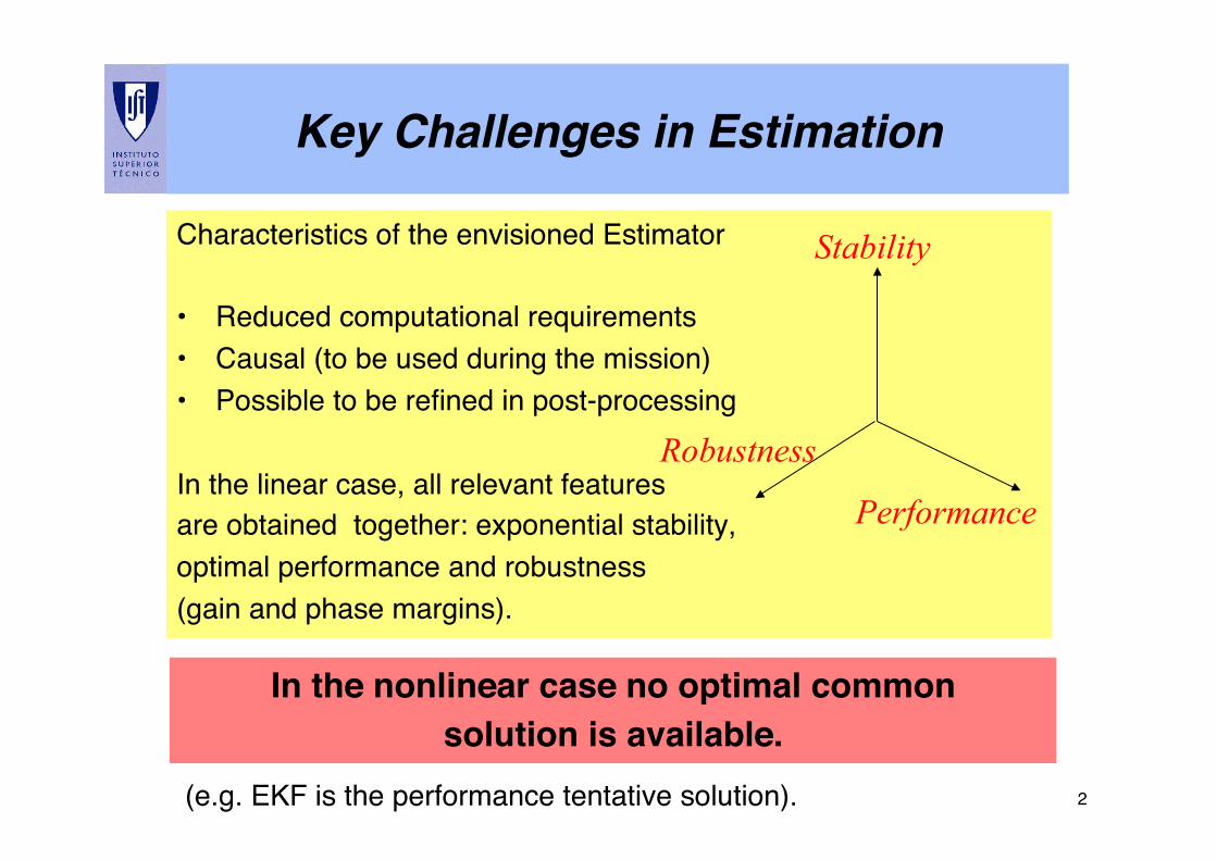
Characteristics of the envisioned Estimator!!• Reduced computational requirements!• Causal (to be used during the mission)!• Possible to be refined in post-processing!!In the linear case, all relevant features !are obtained together: exponential stability, !optimal performance and robustness !(gain and phase margins).!!!
Stability
Performance
Robustness
In the nonlinear case no optimal common!solution is available.!
!(e.g. EKF is the performance tentative solution).!
3!
Theme!
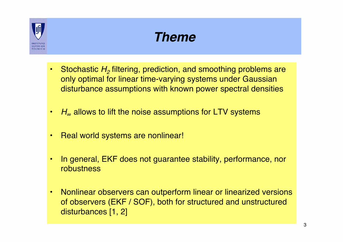
• Stochastic H2 filtering, prediction, and smoothing problems are only optimal for linear time-varying systems under Gaussian disturbance assumptions with known power spectral densities!
• H∞ allows to lift the noise assumptions for LTV systems!
• Real world systems are nonlinear!!!• In general, EKF does not guarantee stability, performance, nor
robustness!
• Nonlinear observers can outperform linear or linearized versions of observers (EKF / SOF), both for structured and unstructured disturbances [1, 2]!
4!
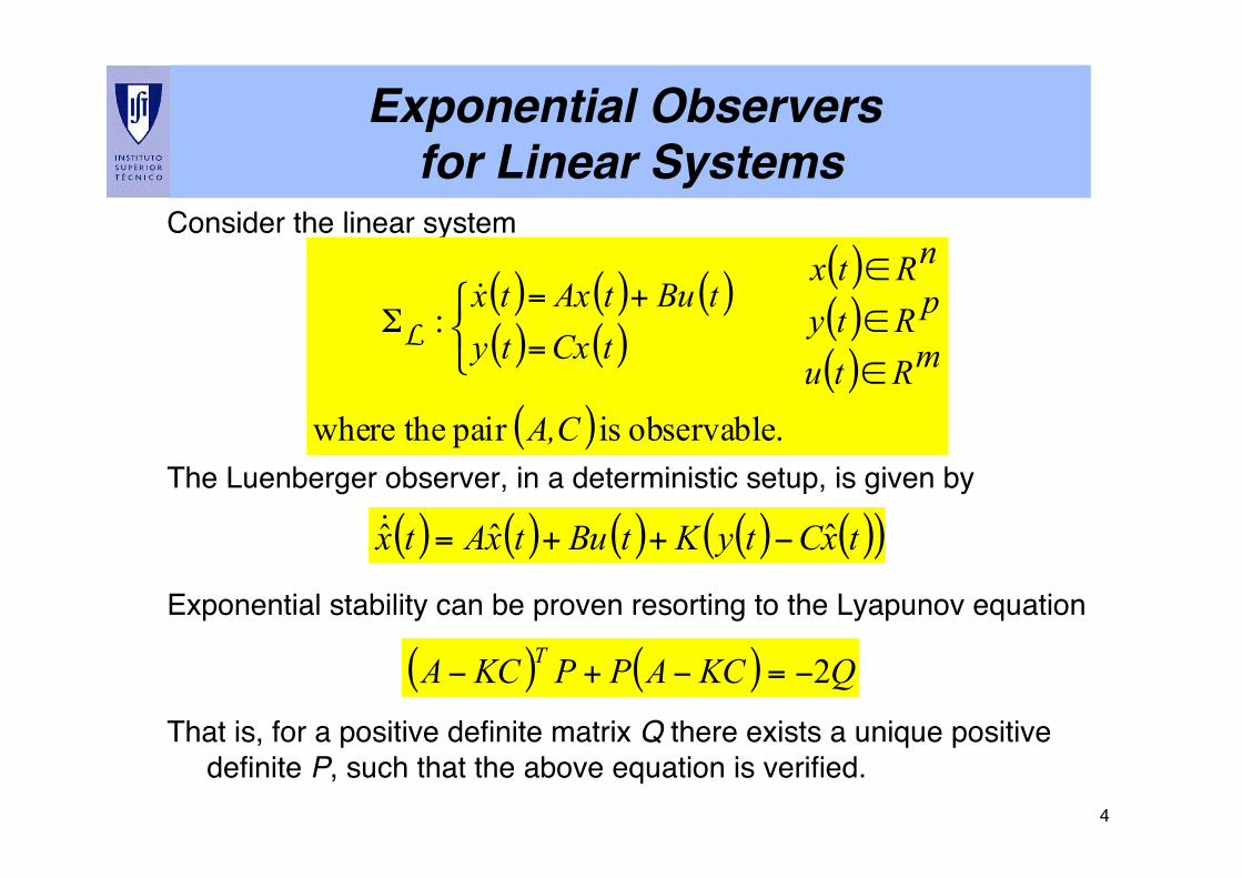
Exponential Observers for Linear Systems!
Consider the linear system !!!!!!The Luenberger observer, in a deterministic setup, is given by !!!Exponential stability can be proven resorting to the Lyapunov equation!!!That is, for a positive definite matrix Q there exists a unique positive
definite P, such that the above equation is verified.!
( )( )
( )( )
( ) ( )( )( )
( ) .observable is pair thewhere
:
A,C
mRtu
pRty
nRtxtBu
tCxtAx
tytx
∈
∈
∈+
=
=Σ
⎩⎨⎧ !
L
( ) ( ) ( ) ( ) ( )( )txCtyKtButxAtx ˆˆˆ −++=!
( ) ( ) QKCAPPKCA T 2−=−+−
5!
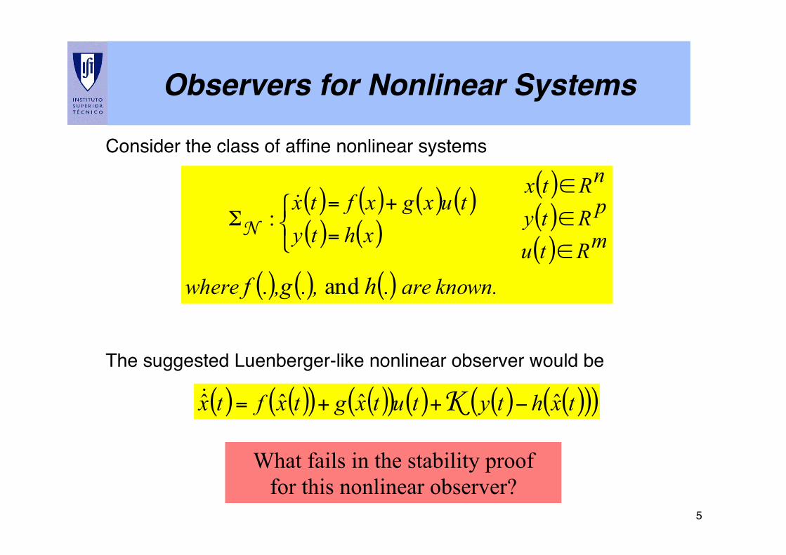
Observers for Nonlinear Systems!
Consider the class of affine nonlinear systems!!!!!!!!The suggested Luenberger-like nonlinear observer would be!! ( ) ( )( ) ( )( ) ( ) ( ) ( )( )( )txhtytutxgtxftx ˆˆˆˆ −++= K!
( )( )
( )( )
( ) ( ) ( )( )( )
( ) ( ) ( ) are known.where
mRtu
pRty
nRtxtuxg
xhxf
tytx
. h, .,g.f and
:∈
∈
∈+
=
=Σ
⎩⎨⎧ !
N
What fails in the stability proof for this nonlinear observer?
6!
Lipschitz Nonlinear Observers!
PAULO OLIVEIRA!!
DEEC/IST and ISR!!
Last Revised: December 14, 2007!Ref. No. NLO#2!
7!
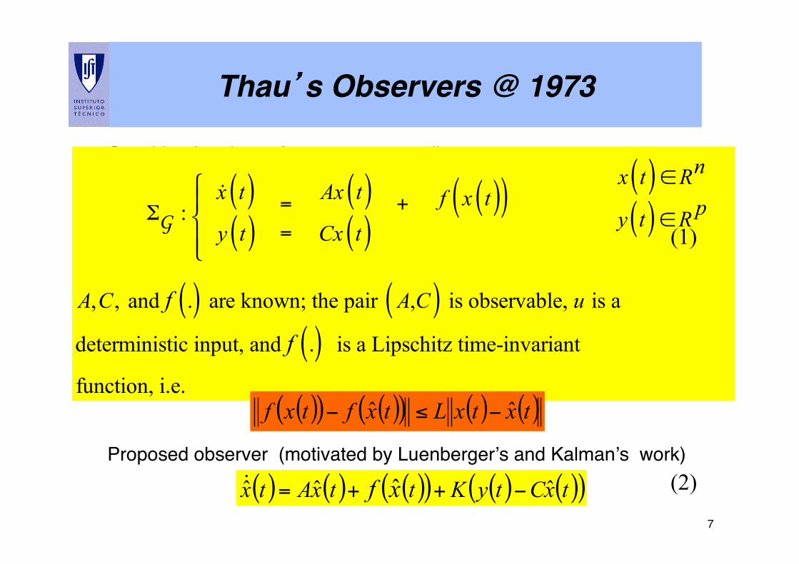
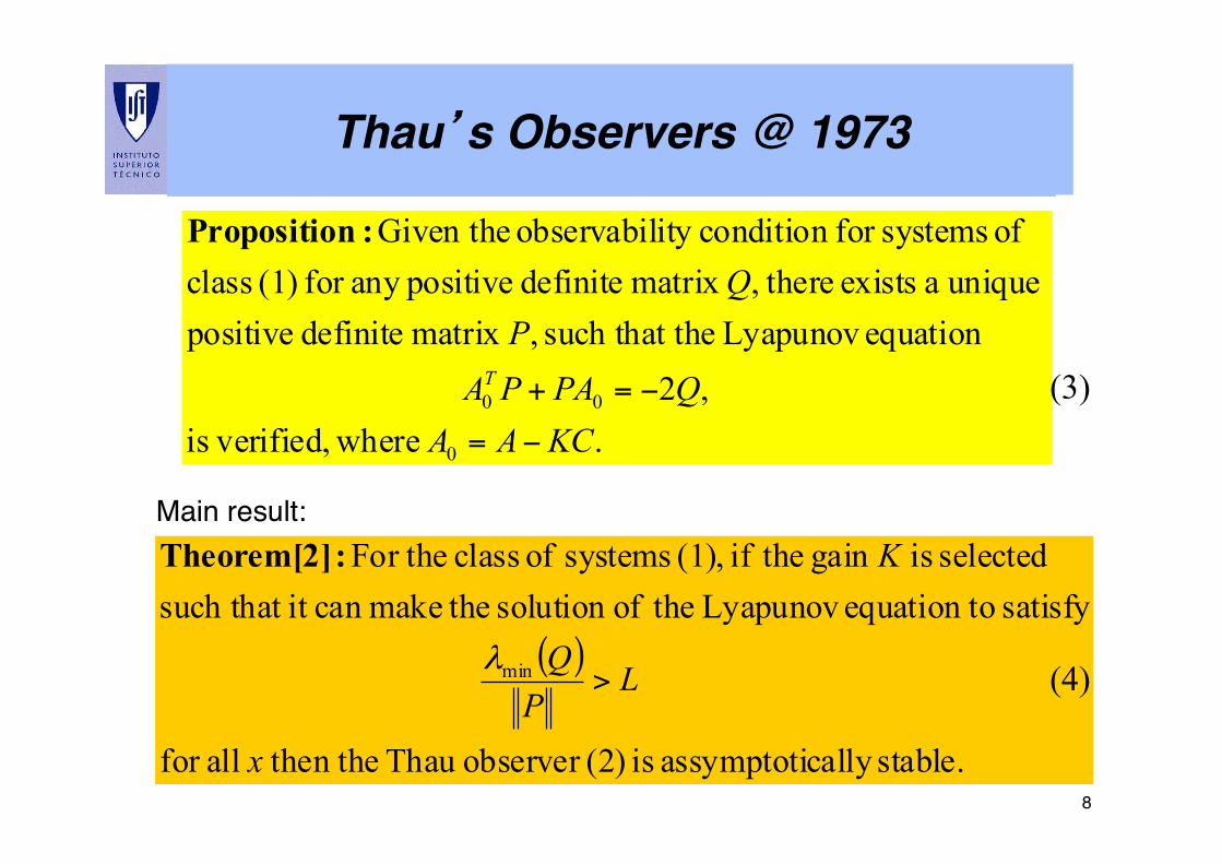
Thau’s Observers @ 1973!
Consider the class of autonomous nonlinear systems !!!!!!!!!!!Proposed observer (motivated by Luenberger’s and Kalman’s work)!!
ΣG :!x t( )y t( )
==
Ax t( )Cx t( )
+ f x t( )( )"#$
%$
x t( )∈Rn
y t( )∈R p
A,C, and f .( ) are known; the pair A,C( ) is observable, u is a
deterministic input, and f .( ) is a Lipschitz time-invariant
function, i.e.
( ) ( ) ( )( ) ( ) ( )( )txCtyKttxAtx xf ˆˆˆ ˆ −++=!
(1) (2)
( )( ) ( )( ) ( ) ( )txtxLtxftxf ˆˆ −≤−
8!
( )
stable.cally assymptoti is (2)observer Thau then the allfor
satisfy oequation t Lyapunov theofsolution themakecan it such that selected is gain theif (1), systems of class For the
min
x
LPQ
K
>λ
:Theorem[2]
. where verified,is,2
equation Lyapunov thesuch that ,matrix definite positive unique a exists there,matrix definite positiveany for (1) class
of systemsfor condition ity observabil Given the
0
00
KCAAQPAPA
PQ
T
−=
−=+
:nPropositio
Main result:!
(3) (4)
Thau’s Observers @ 1973!
9!
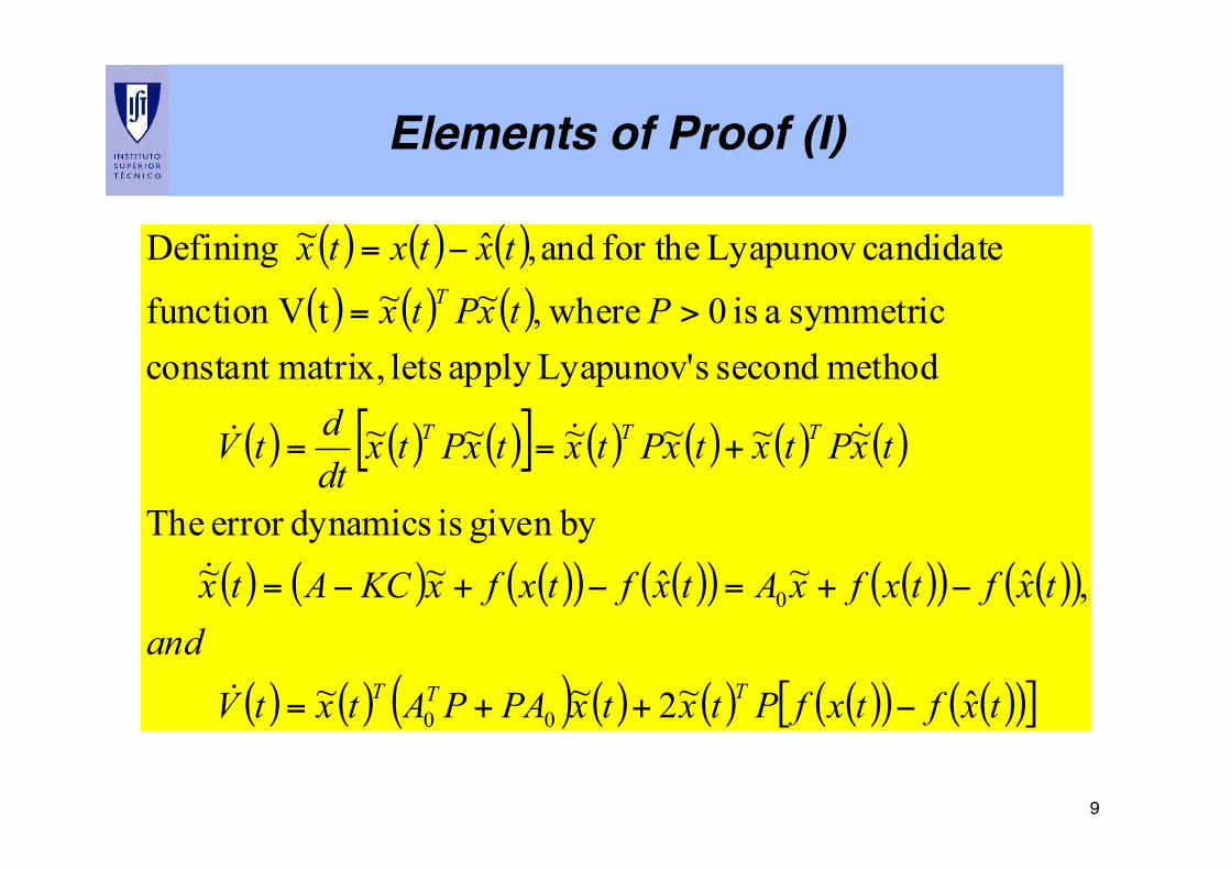
Elements of Proof (I)!
( ) ( ) ( )( ) ( ) ( )
( ) ( ) ( )[ ] ( ) ( ) ( ) ( )
( ) ( ) ( )( ) ( )( ) ( )( ) ( )( )
( ) ( ) ( ) ( ) ( ) ( )( ) ( )( )[ ]txftxfPtxtxPAPAtxtV
andtxftxfxAtxftxfxKCAtx
txPtxtxPtxtxPtxdtdtV
PtxPtx
txtxtx
TTT
TTT
T
ˆ~2~~
,ˆ~ˆ~~by given is dynamicserror The
~~~~~~
method second sLyapunov'apply lets matrix,constant symmetric a is 0 where,~~tVfunction
candidate Lyapunov for the and,ˆ~ Defining
00
0
−++=
−+=−+−=
+==
>=
−=
!
!
!!!
10!
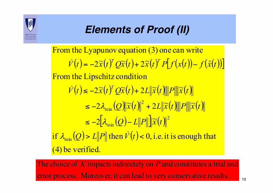
Elements of Proof (II)!
( ) ( ) ( ) ( ) ( )( ) ( )( )[ ]
( ) ( ) ( ) ( ) ( )
( ) ( ) ( ) ( )
( )[ ] ( )( ) ( ) verified.be (4)
t enough tha isit i.e. ,0 then if
~2
~~2~2
~~2~~2
condition Lipschitz theFromˆ~2~~2
can write one (3)equation Lyapunov theFrom
min
2min
2min
<>
−−≤
+−≤
+−≤
−+−=
tVPLQ
txPLQ
txPtxLtxQ
txPtxLtxQtxtV
txftxfPtxtxQtxtV
T
TT
!
!
!
λ
λ
λ
results. veconservati very toleadcan it Moreover, process.error and triala sconstitute and on y indirectel impacts of choice The PK
11!
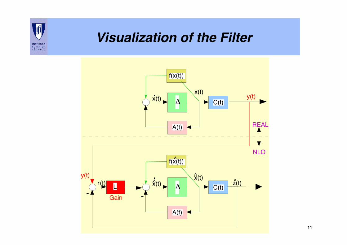
Visualization of the Filter!
x(t) x(t)
Δ y(t) C(t)
A(t)
r (t) x(t) x(t) z(t)
C(t)
A(t)
y(t)
-
.
^ ^
^ .
Gain
REAL
Δ L
f(x(t))
f(x(t)) ^ NLO
12!
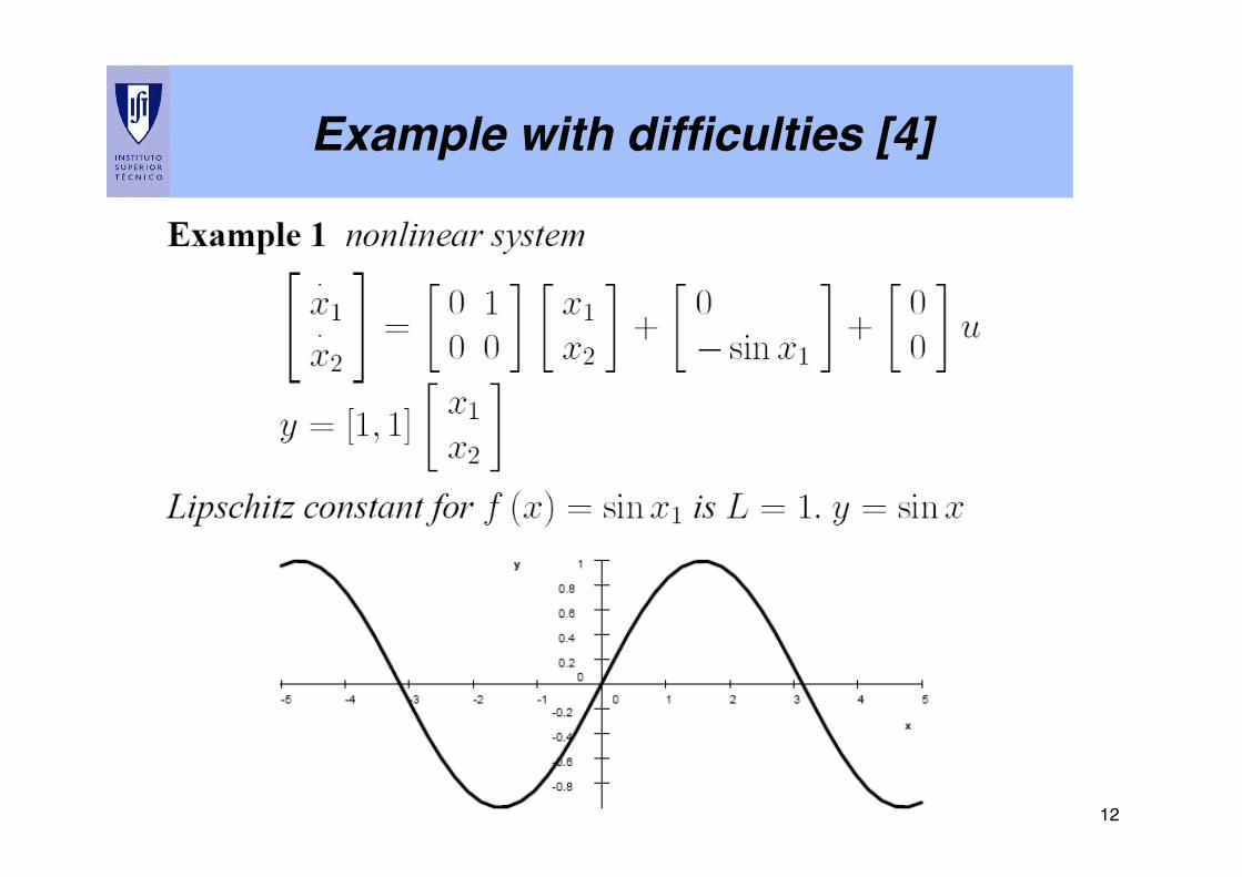
Example with difficulties [4]!
13!
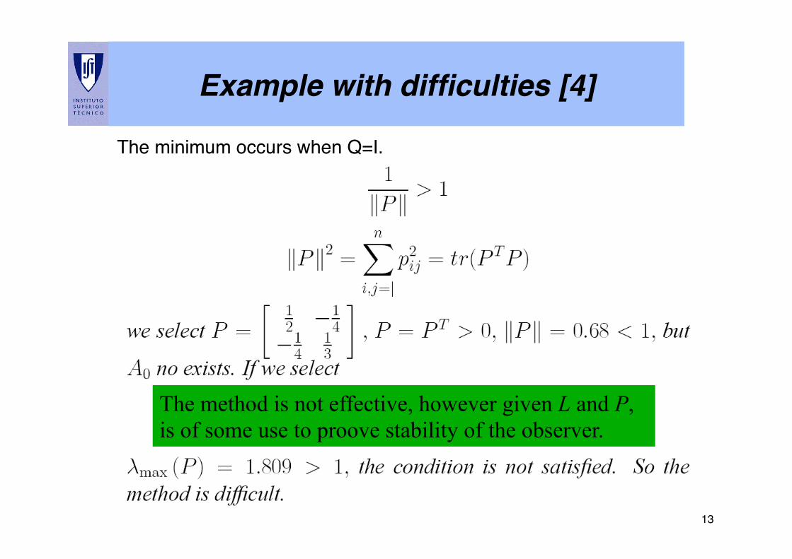
The minimum occurs when Q=I.!
Example with difficulties [4]!
The method is not effective, however given L and P, is of some use to proove stability of the observer.
14!
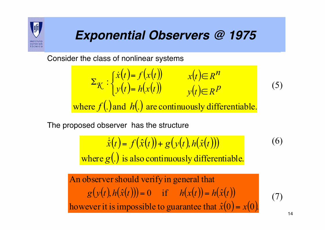
Consider the class of nonlinear systems !!!!!!The proposed observer has the structure!!
( )( )
( )( )( )( )
( )( )
( ) ( ) able.differentily continuous are and where
:
.h.f
pRty
nRtxtxhtxf
tytx
∈
∈=
=Σ
⎩⎨⎧ !
K
( ) ( )( ) ( ) ( )( )( )( ) able.differentily continuous also is . where
ˆ,ˆ ˆg
gxf txhtyttx +=!
(5) (6) (7)
Exponential Observers @ 1975!
( ) ( )( )( ) ( )( ) ( )( )( ) ( ).00ˆ that guarantee toimpossible isit however
ˆ if 0ˆ, thatgeneralin verify shouldobserver An
xxtxhtxhtxhtyg=
==
15!
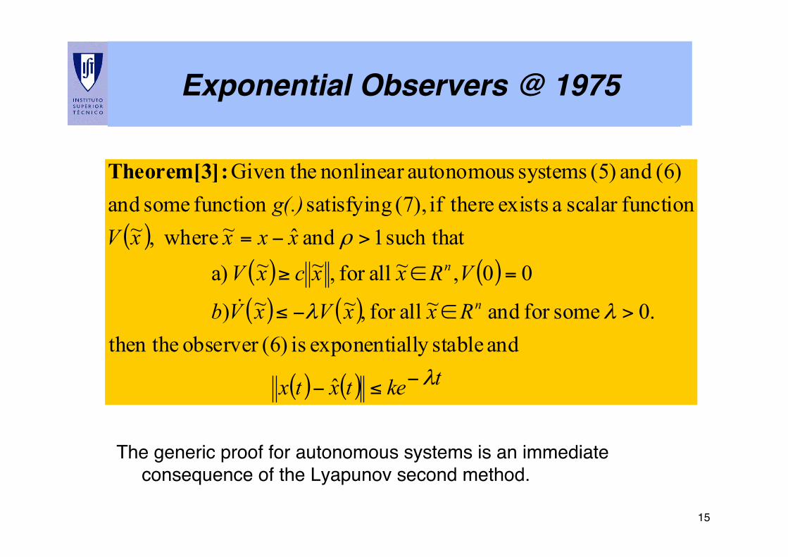
Exponential Observers @ 1975!
( )( ) ( )( ) ( )
( ) ( ) tketxtx
RxxVxVb
VRxxcxVxxxxVg(.)
n
n
λ
λλ
ρ
−≤−
>∈−≤
=∈≥
>−=
ˆ
and stablelly exponentia is (6)observer then the.0 somefor and ~ allfor ,~~)
00,~ allfor ,~~ a)such that 1 and ˆ~ where,~
functionscalar a exists thereif (7), satisfying function some and(6) and (5) systems autonomousnonlinear Given the
!
:Theorem[3]
The generic proof for autonomous systems is an immediate consequence of the Lyapunov second method.!
16!
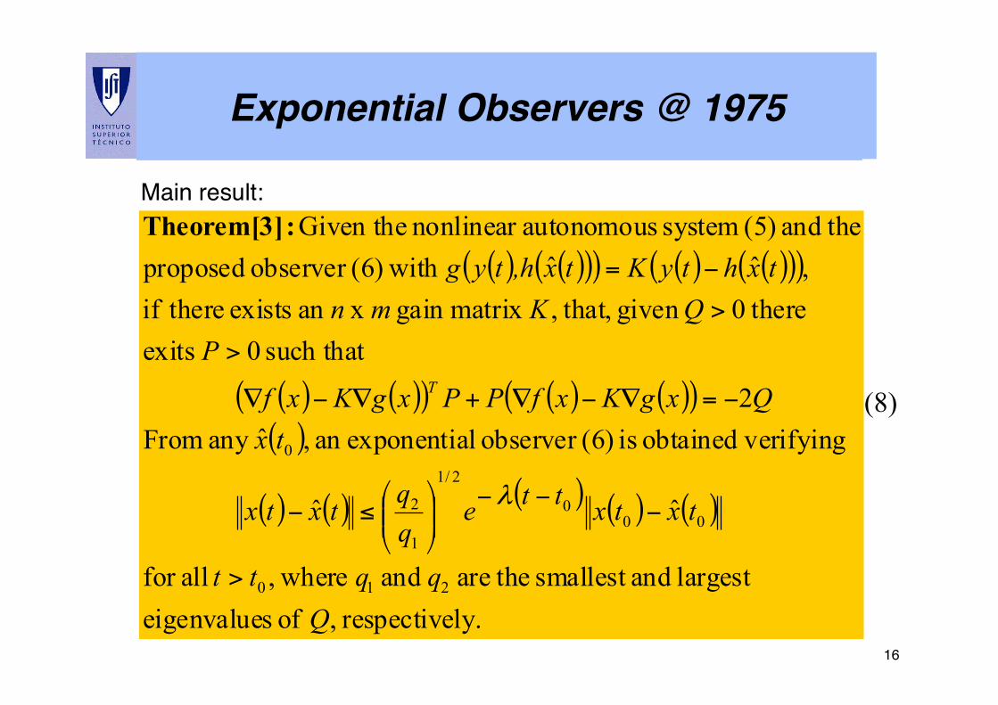
Exponential Observers @ 1975!
( ) ( )( )( ) ( ) ( )( )( )
( ) ( )( ) ( ) ( )( )( )
( ) ( ) ( ) ( ) ( )
ly.respective , of seigenvaluelargest andsmallest theare and where, allfor
ˆˆ
verifyingobtained is (6)observer lexponentiaan ,ˆany From2
such that 0 exits there0given that,,matrix gain x an exists thereif
,ˆˆ with (6)observer proposed theand (5) system autonomousnonlinear Given the
210
000
2/1
1
2
0
Qqqtt
txtxtteqqtxtx
txQxgKxfPPxgKxf
PQKmn
txhtyKtx,htyg
T
>
−−−
⎟⎟⎠
⎞⎜⎜⎝
⎛≤−
−=∇−∇+∇−∇
>
>
−=
λ
:Theorem[3]Main result:!
(8)
17!
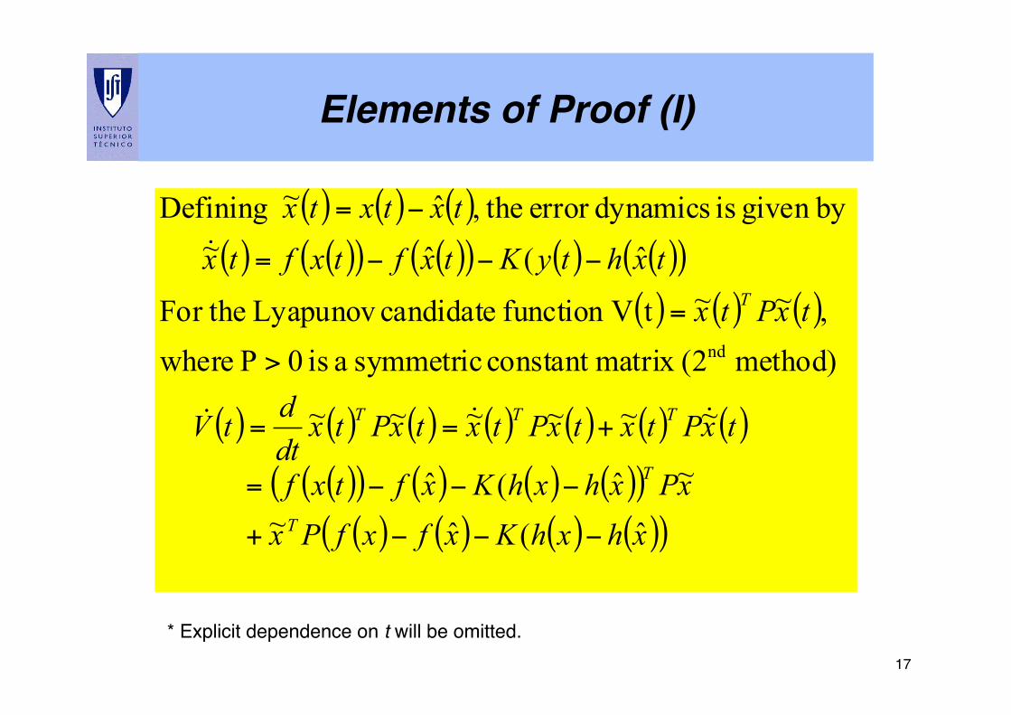
Elements of Proof (I)!
( ) ( ) ( )( ) ( )( ) ( )( ) ( ) ( )( )
( ) ( ) ( )
( ) ( ) ( ) ( ) ( ) ( ) ( )
( )( ) ( ) ( ) ( )( )( ) ( ) ( ) ( )( )xhxhKxfxfPx
xPxhxhKxftxf
txPtxtxPtxtxPtxdtdtV
txPtx
txhtyKtxftxftx
txtxtx
T
T
TTT
T
ˆ(ˆ~~ˆ(ˆ
~~~~~~
method) (2matrix constant symmetric a is 0P where ,~~tVfunction candidate Lyapunov For the
ˆ(ˆ~by given is dynamicserror the,ˆ~ Defining
nd
−−−+
−−−=
+==
>
=
−−−=
−=
!!!
!
* Explicit dependence on t will be omitted. !
18!
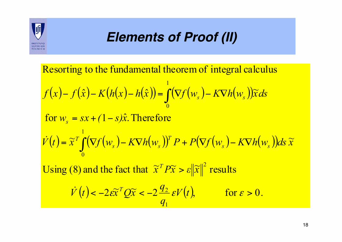
Elements of Proof (II)!
( ) ( ) ( ) ( )( ) ( ) ( )( )
( ) ( ) ( )( ) ( ) ( )( )
( ) ( ) .0for ,2~~2
results ~~~ fact that theand (8) Using
~~
Therefore .ˆ1for
~ˆˆ
calculus integral of theoremlfundamenta the toResorting
1
2
2
1
0
1
0
>−<−<
>
∇−∇+∇−∇=
−+=
∇−∇=−−−
∫
∫
εεε tVqqxQxtV
xεxPx
xdswhKwfPPwhKwfxtV
xs)(sxw
dsxwhKwfxhxhKxfxf
T
T
ssT
ssT
s
ss
!
!
19!
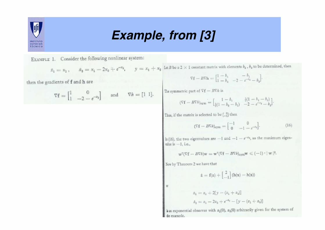
Example, from [3]!
20!
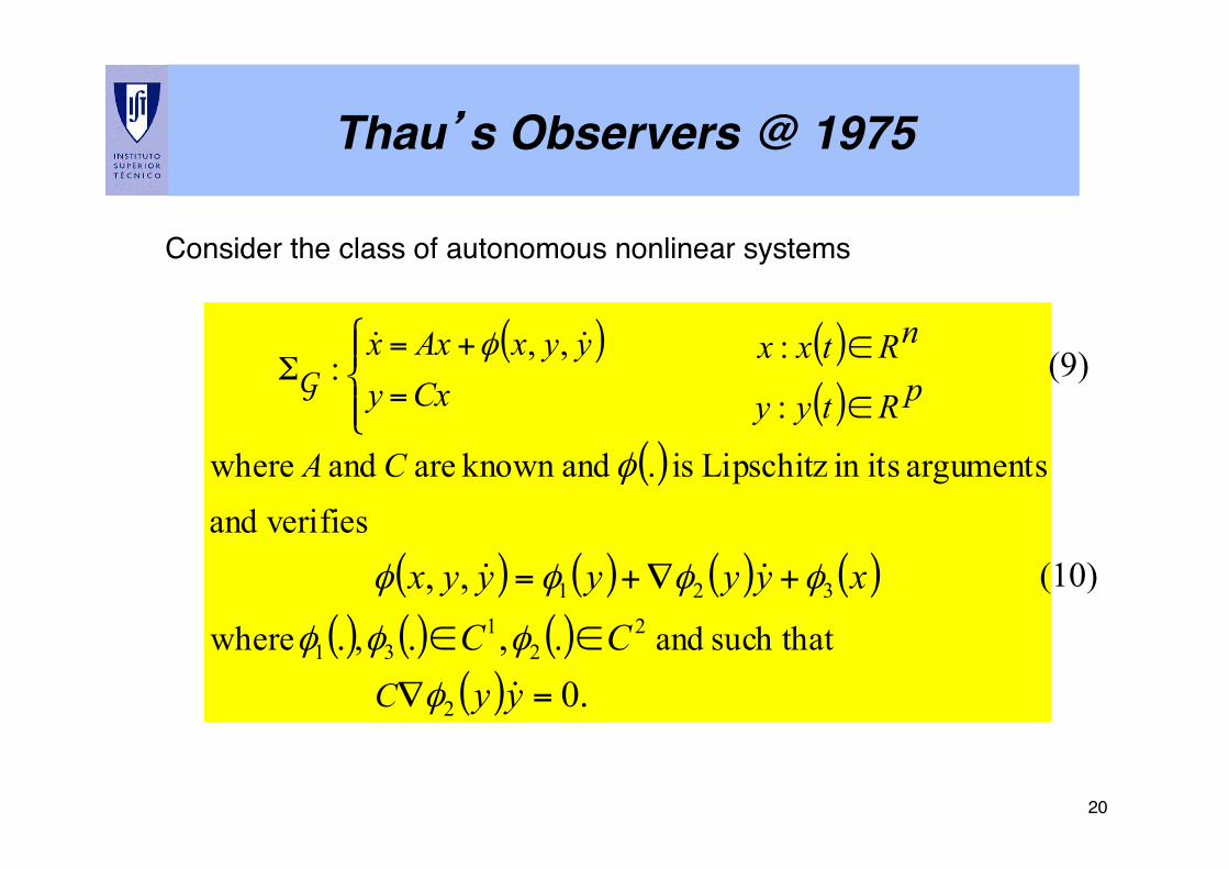
Thau’s Observers @ 1975!
Consider the class of autonomous nonlinear systems !
( ) ( )( )
( )
( ) ( ) ( ) ( )( ) ( ) ( )
( ) .0.,..
,,
2
22
131
321
such that and , where
verifiesandarguments itsin Lipschitz is andknown are and where
:
:,,:
=∇
∈∈
+∇+=
⎪⎩
⎪⎨⎧
∈
∈+
=
=Σ
yyCC
xyyyyyx
.
C
CA
pRtyy
nRtxxyyxCxAx
yx
!
!!
!!
φ
φφφ
φφφφ
φ
φG (9)
(10)
21!
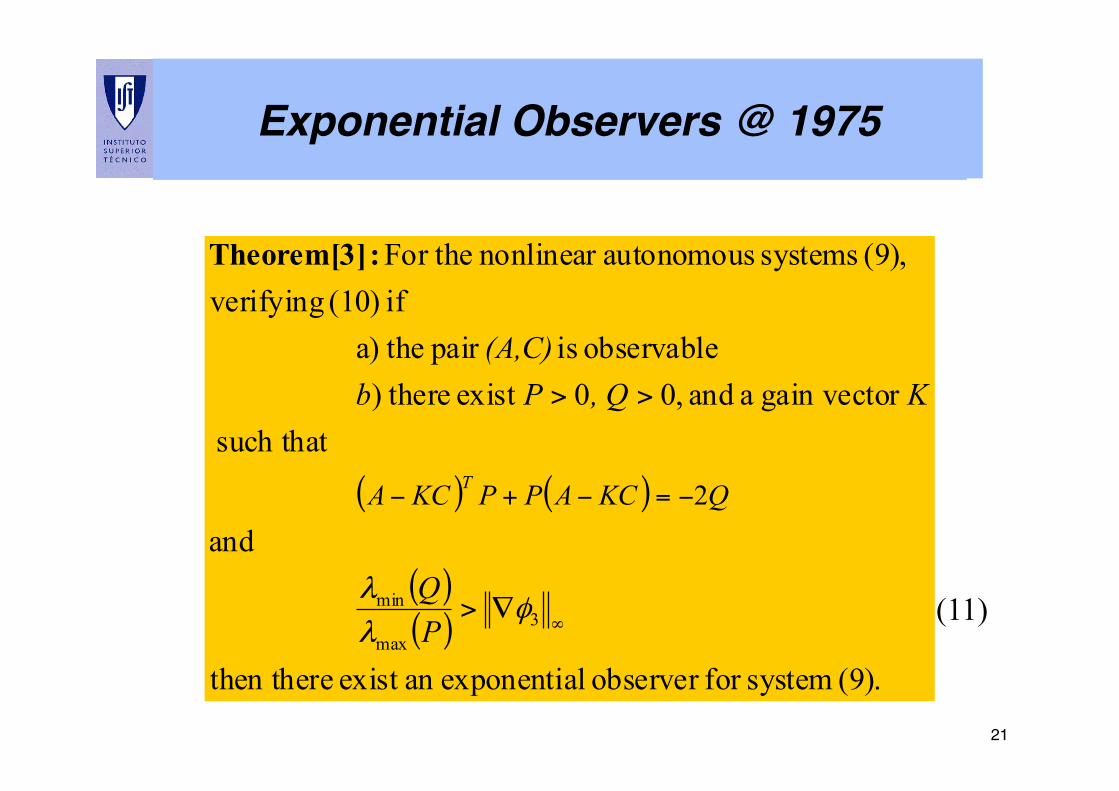
Exponential Observers @ 1975!
( ) ( )
( )( )
(9). systemfor observer lexponentiaan exist then there
and
such that r gain vecto a and ,00exist there)
observable is pair thea)if (10) verifying
(9), systems autonomousnonlinear For the
3max
min
2
∞∇>
>>
−=−+−
φλλ
PQ
K, QPb(A,C)
QKCAPPKCA T
:Theorem[3]
(11)
22!
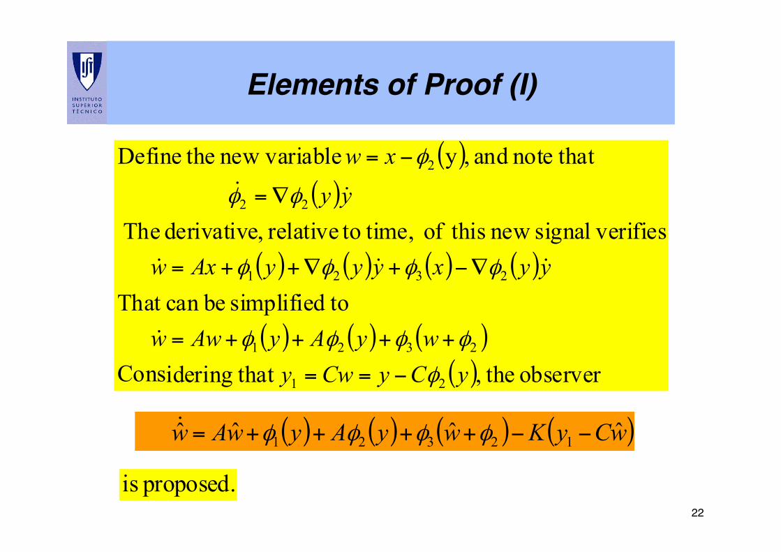
Elements of Proof (I)!
( )( )
( ) ( ) ( ) ( )
( ) ( ) ( )( ) observer the, that ideringCons
tosimplified becan That
verifiessignal new thisof time, torelative ,derivative The
thatnote and ,y variablenew theDefine
21
2321
2321
22
2
yCyCwywyAyAww
yyxyyyAxw
yy
xw
φ
φφφφ
φφφφ
φφ
φ
−==
++++=
∇−+∇++=
∇=
−=
!
!!!
!!
( ) ( ) ( ) ( )wCyKwyAywAw ˆˆˆˆ 12321 −−++++= φφφφ!
proposed. is
23!
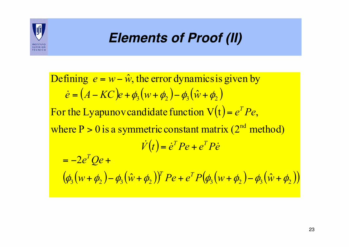
Elements of Proof (II)!
( ) ( ) ( )( )
( )
( ) ( )( ) ( ) ( )( )23232323
nd
2323
ˆˆ
2
method) (2matrix constant symmetric a is 0P where ,tVfunction candidate Lyapunov For the
ˆby given is dynamicserror the,ˆ Defining
φφφφφφφφ
φφφφ
+−+++−+
+−=+=
>
=
+−++−=
−=
wwPePeww
QeeePePeetV
PeewweKCAe
wwe
TT
T
TT
T
!!!
!
24!
Elements of Proof (III)!
( ) ( )( )
( )( )
( )[ ] 23min
1
023
1
023min
22
2
ePQ
dseywPe
PedseywQV
sT
T
s
∞∇+−≤
⎟⎟⎠
⎞⎜⎜⎝
⎛+∇+
⎟⎟⎠
⎞⎜⎜⎝
⎛+∇+−≤
∫
∫
φλ
φφ
φφλ!
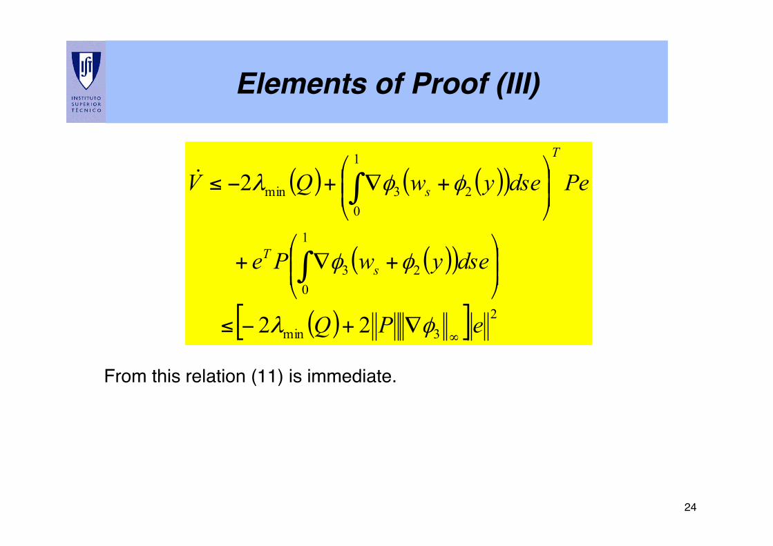
From this relation (11) is immediate.!
25!
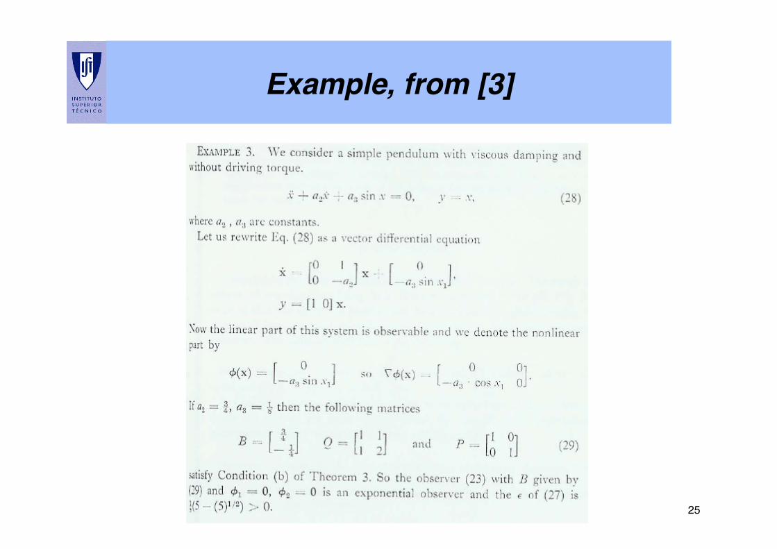
Example, from [3]!
26!
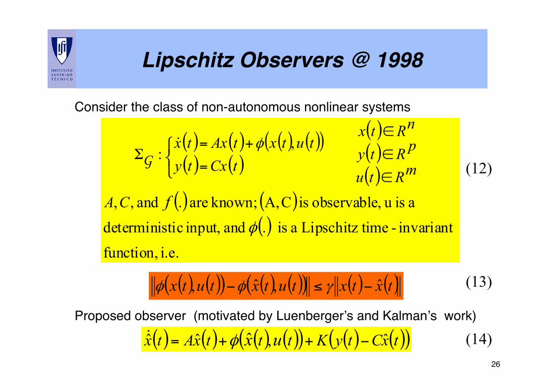
Lipschitz Observers @ 1998!
Consider the class of non-autonomous nonlinear systems !!!!!!!!!!!Proposed observer (motivated by Luenberger’s and Kalman’s work)!!
( )( )
( )( )
( ) ( )( ) ( )( )( )
( ) ( )( )
i.e. function,invariant - timeLipschitz a is and input, ticdeterminis
a isu ,observable is CA, known; are and ,,
,:
..fCA
mRtu
pRty
nRtxtutx
tCxtAx
tytx
φ
φ
∈
∈
∈+
=
=Σ
⎩⎨⎧ !
G
( ) ( ) ( ) ( )( ) ( ) ( )( )txCtyKtttxAtx ux ˆ,ˆˆ ˆ −++= φ!
(12) (13) (14)
( ) ( )( ) ( ) ( )( ) ( ) ( )txtxtutxtutx ˆ,ˆ, −≤− γφφ
27!
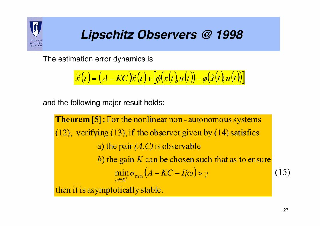
( )
stable.ally asymptotic isit then
minensure toassuch that chosen becan gain the)
observable is pair thea)satisfies (14)by given observer theif (13), g verifyin(12),systems autonomous-nonnonlinear For the
min γIjωKCAσKb(A,C)
Rω>−−
+∈
:[5] Theorem
(15)
Lipschitz Observers @ 1998!
( ) ( ) ( ) ( ) ( )( ) ( ) ( )( )[ ]tutxtutxtxKCAtx ,ˆ,~~ φφ −+−=!
The estimation error dynamics is!!!!and the following major result holds:!!
28!
Elements of Proof (I)!
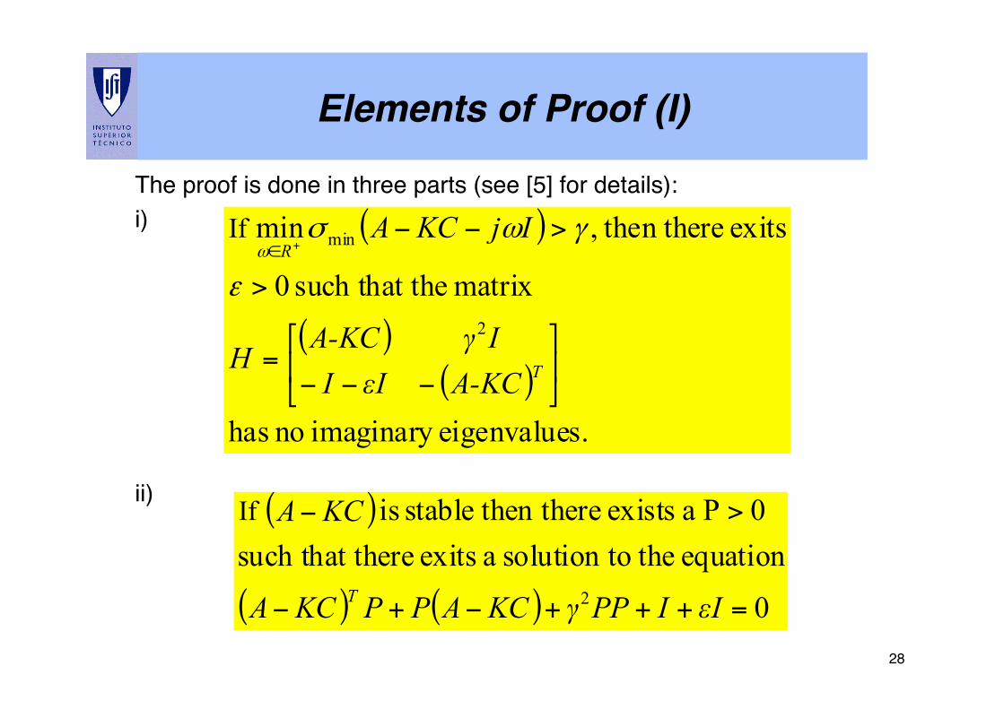
The proof is done in three parts (see [5] for details):!i)!!!!!!!!ii) !
( )
( )( )
s.eigenvalueimaginary no has
matrix thesuch that 0
exits e then ther,min
2
min If
⎥⎦
⎤⎢⎣
⎡
−−−=
>
>−−+∈
T
R
A-KCεIIIγA-KC
H
IjKCA
ε
γωσω
( )
( ) ( ) 0
equation theosolution t a exits theresuch that 0P a exists e then therstable is
2
If
=+++−+−
>−
εIIPPγKCAPPKCA
KCA
T
29!
Elements of Proof (II)!
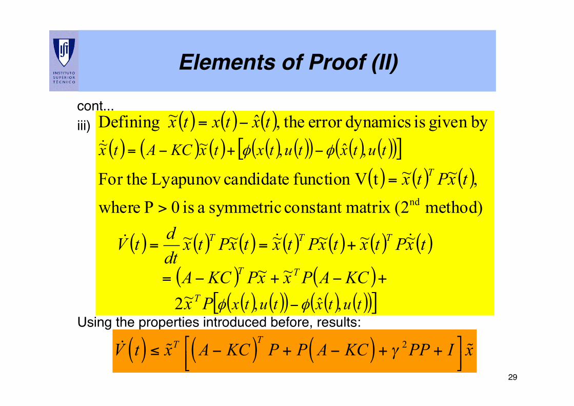
cont...!iii)!!!!!!!!!!Using the properties introduced before, results:!!!!!
( ) ( ) ( )( ) ( ) ( ) ( ) ( )( ) ( ) ( )( )[ ]
( ) ( ) ( )
( ) ( ) ( ) ( ) ( ) ( ) ( )
( ) ( )( ) ( )( ) ( ) ( )( )[ ]tutxtutx
tutxtutxtxKCAtx
PxKCAPxxPKCA
txPtxtxPtxtxPtxdtdtV
txPtx
txtxtx
T
TT
TTT
T
,ˆ,
,ˆ,~~
~2
~~
~~~~~~
method) (2matrix constant symmetric a is 0P where ,~~tVfunction candidate Lyapunov For the
by given is dynamicserror the,ˆ~ Defining
nd
φφ
φφ
−
−+−=
+−+−=
+==
>
=
−=
!!!
!
!V t( ) ≤ "xT A− KC( )T P + P A− KC( ) + γ 2 PP + I$
%&'()"x
30!
References!
[1] P. Kokotovic , The Joy of Feedback: Nonlinear and Adaptive, Macmillan Press, 1991 Bode Prize Lecture, 1992.!
![2] F. Thau, ”Observing the state of nonlinear dynamical systems,”
International Journal of Control, pp. 471-479, 1973. !![3] S. Kou, D. Elliot, and T. Tarn, ”Exponential observers for
nonlinear dynamic systems,” Journal of Information and Control pp. 204-216, 1975. !
![4] Wen Yu, ”Nonlinear Observer,” class notes, CINVESTAV-IPN.!![5] R. Rajamani, ”Observers for Lipschitz Nonlinear Systems,”
Transactions on Automatic Control, pp. 397-400, 1998.!!
1!
Nonlinear Observers with Linearizable Error Dynamics!
PAULO OLIVEIRA!!
DEEC/IST and ISR!!
Last Revised: January 8, 2007!Ref. No. NLO#3!
2!
Theme!
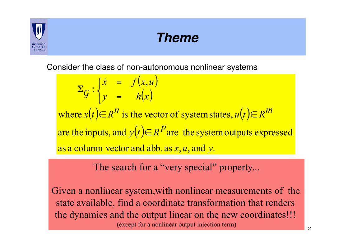
The search for a “very special” property...
Given a nonlinear system,with nonlinear measurements of the state available, find a coordinate transformation that renders the dynamics and the output linear on the new coordinates!!!
(except for a nonlinear output injection term)
( )( )
( ) ( )( )
. and ,, as abb. andtor column vec a as expressed outputs system theare and inputs, theare
,states system of vector theis where
,:
yux
pRty
mRtunRtx
xhyuxfx
∈
∈∈
=
=Σ
⎩⎨⎧ !
G
Consider the class of non-autonomous nonlinear systems !
3!
Theme!
• Challenge for the control problem set at IFAC 1978 (Helsinki) by Roger Brockett to Arthur Krener [1]!
• Control problem well understood (during the 80s), see [1, 2] for a survey on the new techniques: feedback linearization, input-output linearization, backstepping , zero dynamics, …!
• Harder to be solved for nonlinear observers!
Relevant questions:!• Conditions for the existence of such transformation!
• Synthesis methods (complexity)!
• Robustness relative to unmodelled dynamics...!!!!!
4!
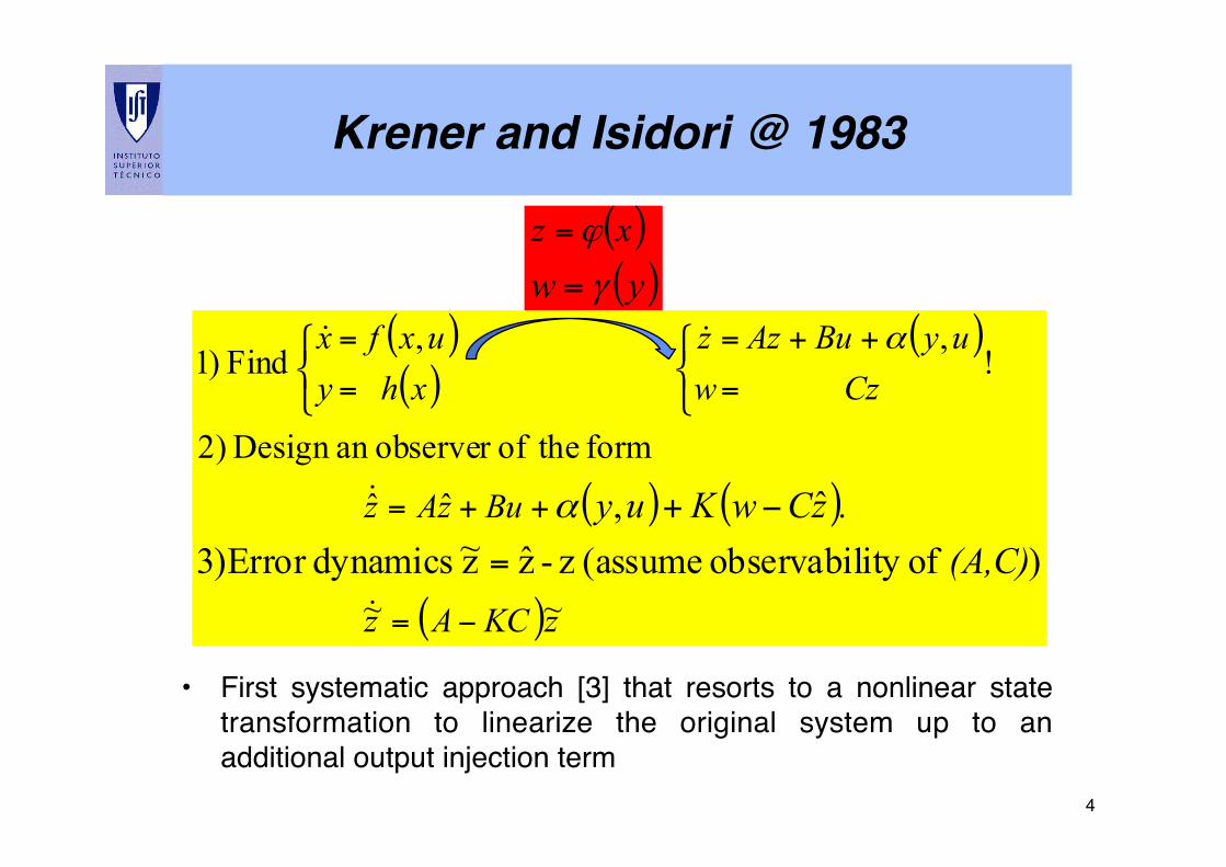
• First systematic approach [3] that resorts to a nonlinear state transformation to linearize the original system up to an additional output injection term!
Krener and Isidori @ 1983!
( )( )
( )
( ) ( )
( )zKCAz
BuzAz
CzuyBuAz
wz
xhuxf
yx
(A,C).zCwKuy
~~
ˆˆ
form theofobserver an Design 2)
!,,
Find )1
) ofity observabil (assume z-zz~ dynamicsError )3ˆ,
−=
++=
++
=
=
=
=
=
−+
⎩⎨⎧
⎩⎨⎧
!
!
!!
α
α
( )( )ywxz
γ
ϕ
=
=
5!
Krener and Isidori @ 1983!
The proposed solution proposed is composed of three steps (see [1, 3] for details):!
!
1) A set of partial differential equations (PDE) must be solved to find γ(y)!
2) The integrability of conditions for this PDE involve the vanishing of a pseudo-curvature!
3) A coordinate transformation z=φ(x) can be obtained after a set of PDEs is solved, resorting to conditions on the Lie derivatives of the outputs!
“The process is more complicated then feedback linearization and even less likely to be successful...” in [1]!
6!
Kazantzis and Kravaris @ 1997!
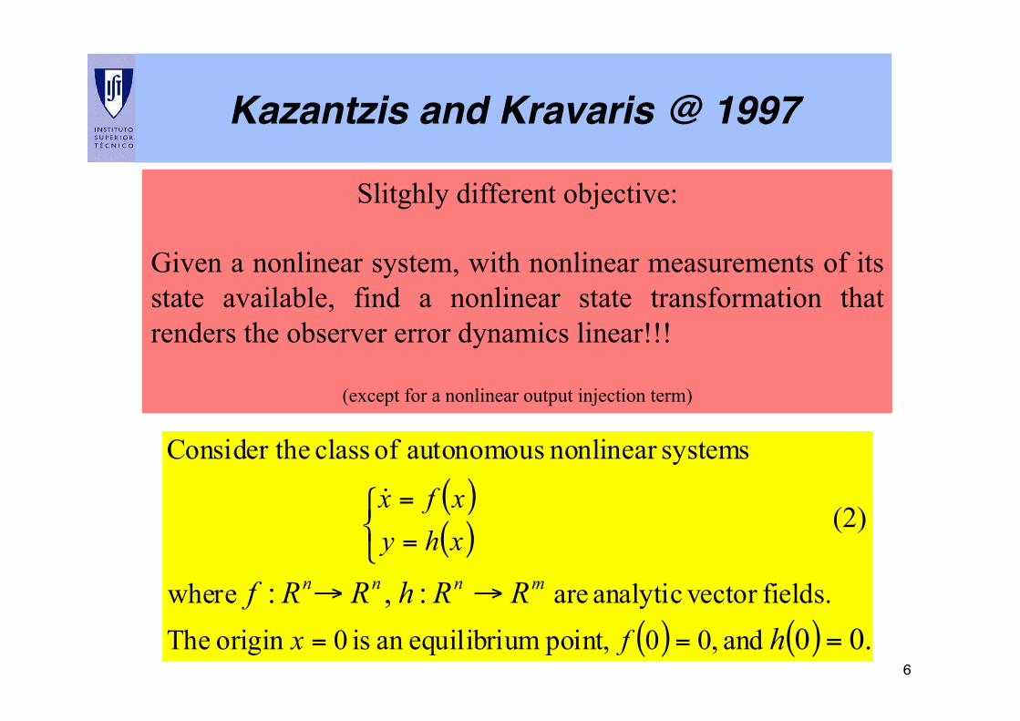
Slitghly different objective:
Given a nonlinear system, with nonlinear measurements of its state available, find a nonlinear state transformation that renders the observer error dynamics linear!!!
(except for a nonlinear output injection term)
( )( )
( ) ( ) .00 :,:
and ,00 point, mequilibriuan is 0origin Thefields. vector analytic are where
systemsnonlinear autonomous of class heConsider t
=
→→
⎩⎨⎧
==
=
=
hRRhRRf
fx
xhyxfx
mnnn
!(2)
7!
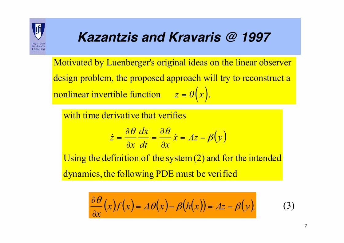
Kazantzis and Kravaris @ 1997!
Motivated by Luenberger's original ideas on the linear observer
design problem, the proposed approach will try to reconstruct a
nonlinear invertible function z = θ x( ).
( )
verifiedbemust PDE following thedynamics,intended for the and (2) system theof definition theUsing
fies that veriderivative with time
yAzxxdt
dxx
z βθθ
−=∂
∂=
∂
∂= !!
( ) ( ) ( ) ( )( ) ( ),yAzxhxAxfxx
ββθθ
−=−=∂
∂ (3)
8!
Kazantzis and Kravaris @ 1997!
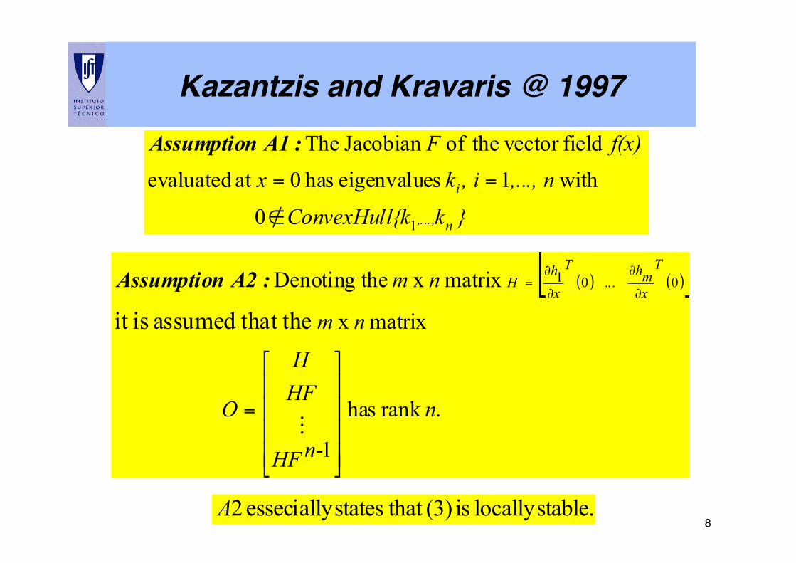
}k{kConvexHull
,..., n, ikxf(x)F
n,...,
i
10
with 1 seigenvalue has 0at evaluated field vector theof Jacobian The
∉
==
:A1 Assumption
( ) ( )[ ]
.rank has
1
matrix x
matrix x theDenoting
that theassumed isit
001
n
n-HF
HFH
O
nm
nmT
xmh...
T
xh
H
⎥⎥⎥⎥
⎦
⎤
⎢⎢⎢⎢
⎣
⎡
=
∂
∂
∂
∂=
!
:A2 Assumption
stable.locally is (3) that states essecially 2A
9!
Kazantzis and Kravaris @ 1997!
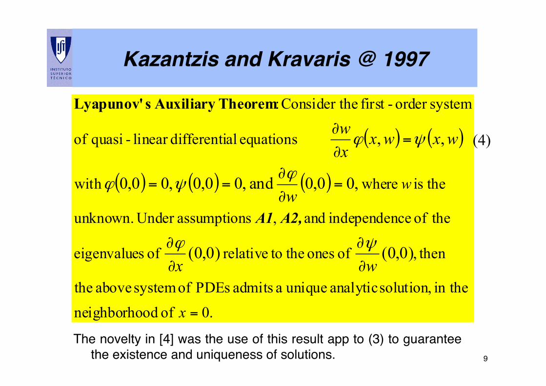
( ) ( )
( ) ( ) ( )
.0 of odneighborho in the solution, analytic unique a admits PDEs of system above the
then , of ones the torelative of seigenvalue
theof ceindependen and , sassumption Under unknown.
theis wherewith
equations aldifferentilinear -quasi of
systemorder -first heConsider t :
(0,0) (0,0)
,00,0 and 0,0,0 0,0,0
,,
=
∂
∂
∂
∂
=∂
∂==
=∂
∂
x
w
wx
w
wxwxxw
ψϕ
ϕψϕ
ψϕ
A2,A1
Theorem AuxiliarysLyapunov'
The novelty in [4] was the use of this result app to (3) to guarantee the existence and uniqueness of solutions.!
(4)
10!
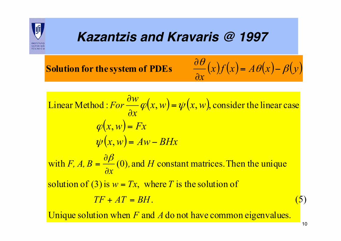
Kazantzis and Kravaris @ 1997!
( ) ( ) ( ) ( )yxAxfxx
βθθ
−=∂
∂ PDEs of system thefor Solution
( ) ( )
( )( )
s.eigenvaluecommon havenot do and hen solution w Unique.
ofsolution theis where, is (3) ofsolution
unique Then the matrices.constant and )0( with
caselinear heconsider t :MethodLinear
,,
,,,
AFBHATTF
TTxw
H,x
BA,F,
For
BHxAwwxFxwx
wxwxxw
=+
=∂
∂=
−=
=
=∂
∂
β
ψ
ϕ
ψϕ
(5)
11!
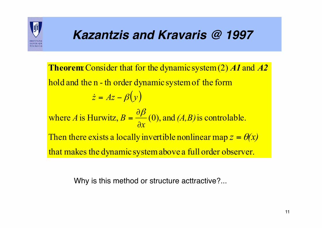
Kazantzis and Kravaris @ 1997!
( )
observer.order full a above system dynamic themakesthat mapnonlinear invertiblelocally a exists Then there
e.controlabl is and ),0( Hurwitz, is where
form theof system dynamicorder th -n theand hold and (2) system dynamic for thehat Consider t :
(x)z
(A,B)x
BA
yAzz
θ
β
β
=∂
∂=
−=!
A2A1Theorem
Why is this method or structure acttractive?...!
12!
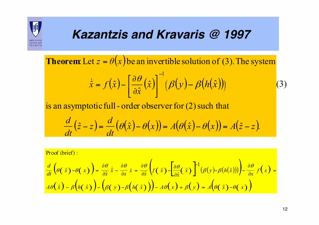
Kazantzis and Kravaris @ 1997!
(3)
( )
( ) ( ) ( ) ( )( )
( ) ( ) ( )( ) ( ) ( )( ) ( ).ˆˆˆˆ
such that (2)for observer order -full asymptotican is
ˆˆ
ˆˆ
system The (3). ofsolution invertiblean be Let :
ˆ1
zzAxxAxxdtdzz
dtd
xx
xfx
xθz
xhy
−=−=−=−
∂
∂−=
=
⎟⎠⎞⎜
⎝⎛
−
−⎥⎦⎤
⎢⎣⎡
θθθθ
θββ!
Theorem
( ) ( )( ) ( ) ( )[ ] ( ) ( )( )( )( ) ( )
( ) ( )( ) ( ) ( )( )( ) ( ) ( ) ( ) ( )( )xxAyxAxhyxhxA
xfxxhyxx
xfxxxxxxxdtd
θθβθβββθ
θββ
θθθθθθ
−=+−−−−
=∂∂
−−−
∂∂
−∂∂
=∂∂
−∂∂
=−
ˆˆˆˆ
ˆ1
ˆˆ
ˆˆˆˆˆ
:(brief) Proof
!!
13!
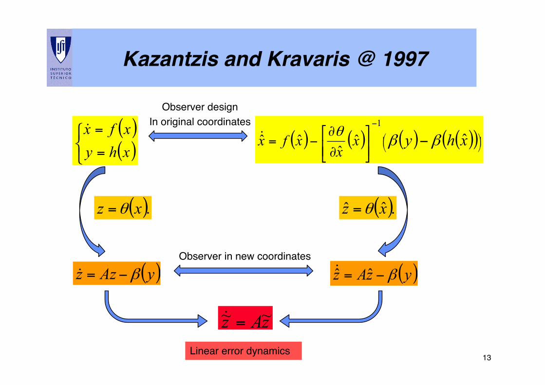
Kazantzis and Kravaris @ 1997!
( )( )⎩
⎨⎧
=
=
xhyxfx!
( ).xz θ=
( )yAzz β−=!
( ) ( ) ( ) ( )( )⎟⎠⎞⎜⎝⎛
−
−⎥⎦⎤
⎢⎣⎡∂
∂−= xhyx
xxfx ˆ
1
ˆˆ
ˆˆ ββθ!
( ).ˆˆ xz θ=
( )yzAz β−= ˆ!
zAz ~~ =!
Observer design!In original coordinates!
Observer in new coordinates!
Linear error dynamics!
14!
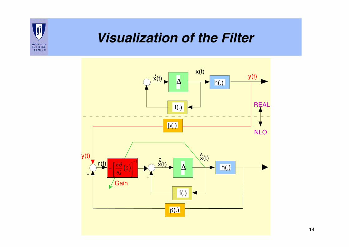
Visualization of the Filter!
x(t) x(t)
Δ y(t)
r (t) x(t) x(t) y(t)
-
.
^ ^ .
Gain
REAL
Δ
f(.)
NLO
f(.)
h(.)
h(.) ( )1
ˆˆ
−
⎥⎦⎤
⎢⎣⎡∂
∂− x
xθ
β(.)
β(.)
15!
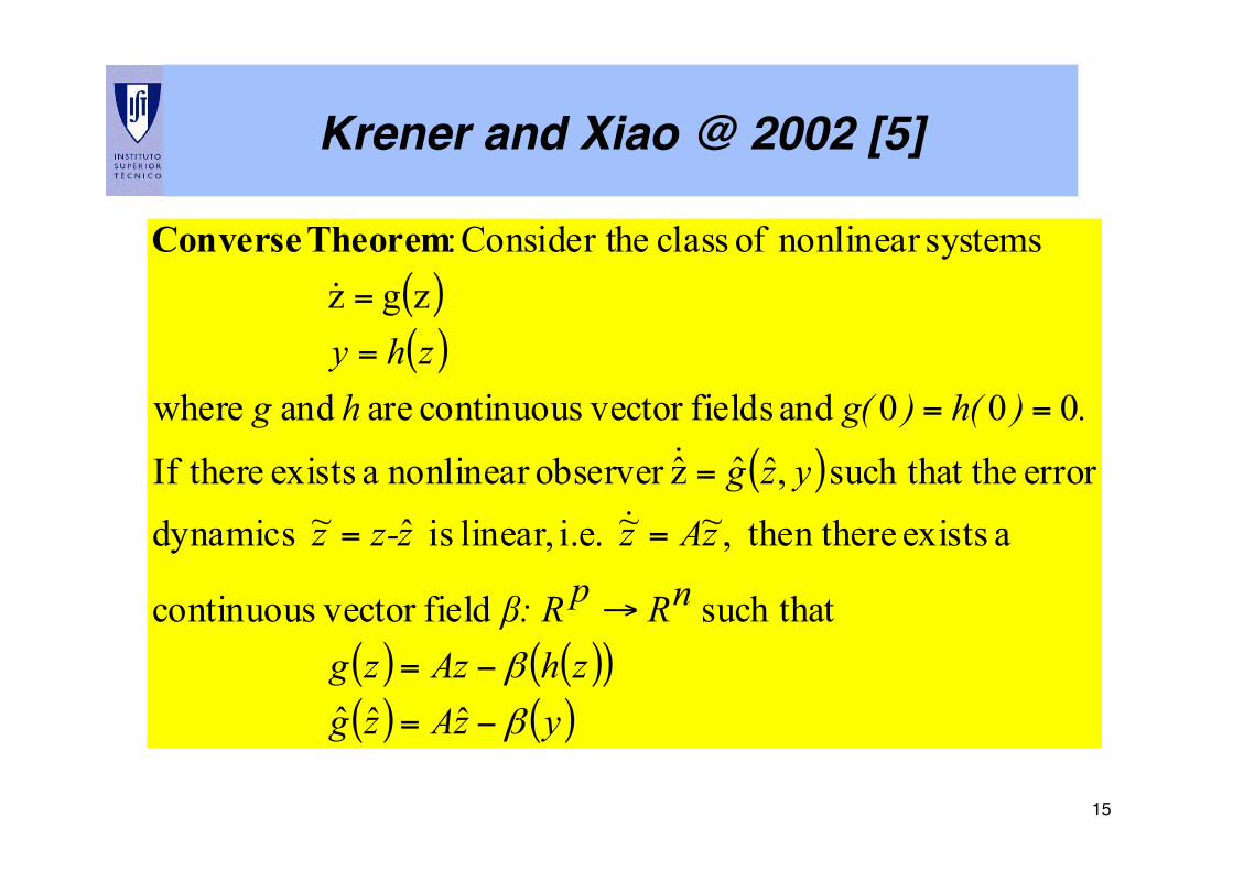
Krener and Xiao @ 2002 [5]!
( )( )
( )
( ) ( )( )( ) ( )yzAzg
zhAzzg
nRpβ: R
zAzzz-z
yzg
.)h()g(hgzhy
β
β
−=
−=
→
==
=
==
=
=
ˆˆˆ
such that field vector continuous
a exists re then the,~~ i.e. linear, is ˆ~ dynamics
error thesuch that ,ˆˆzobserver nonlinear a exists thereIf
000 and fields vector continuous are and where
zgz systemsnonlinear of class heConsider t :
!
!
!Theorem Converse
16!
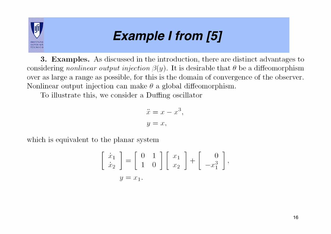
Example I from [5]!
17!
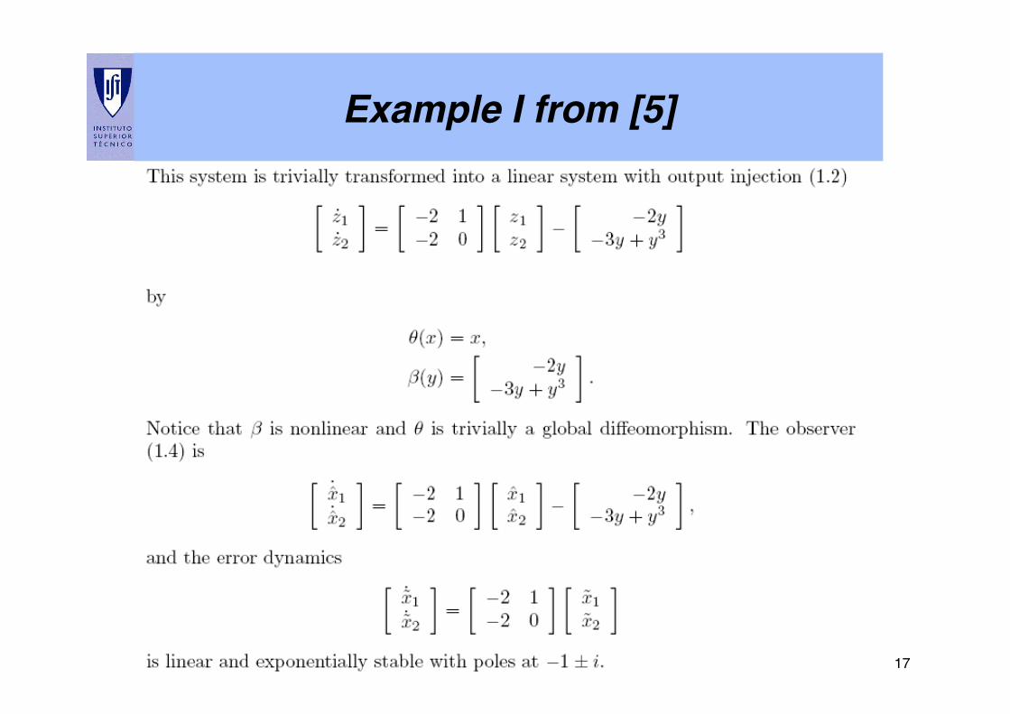
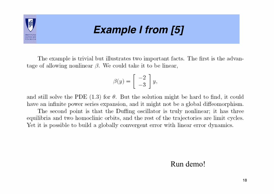
Example I from [5]!
18!
Example I from [5]!
Run demo!
19!
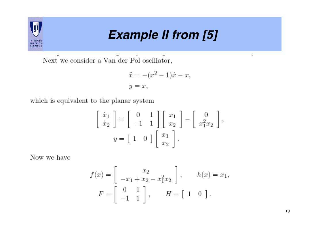
Example II from [5]!
20!
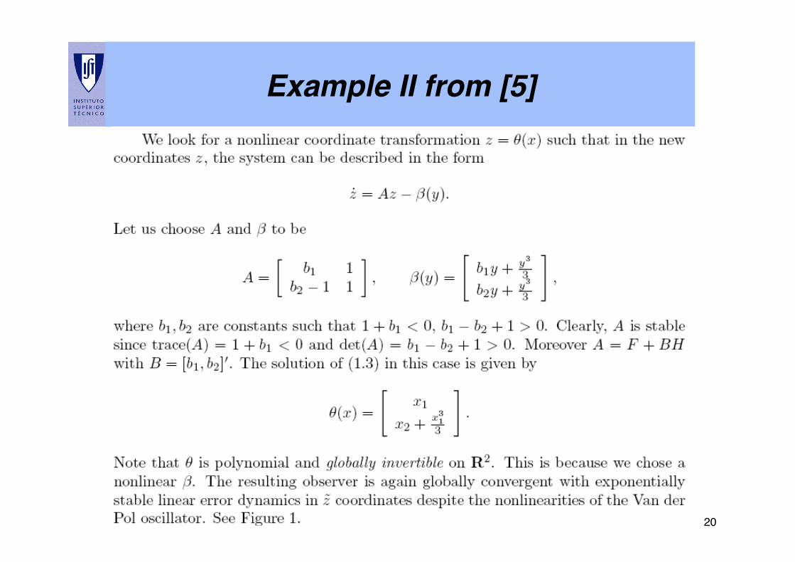
Example II from [5]!
21!
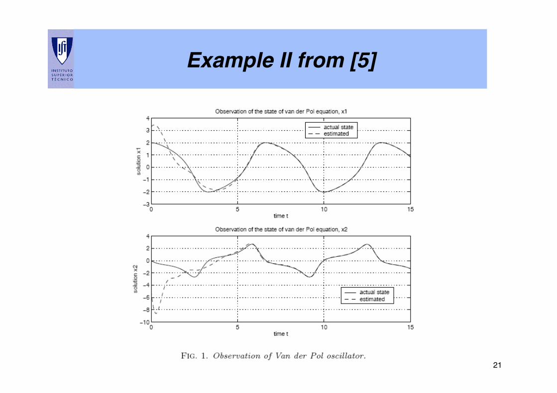
Example II from [5]!
22!
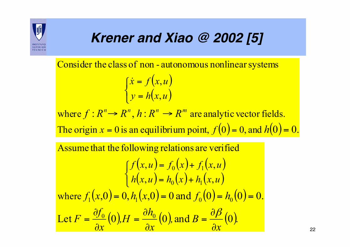
Krener and Xiao @ 2002 [5]!
( )( )
( ) ( ) .00 :,:
and ,00 point, mequilibriuan is 0origin Thefields. vector analytic are where
,,
systemsnonlinear autonomous-non of class heConsider t
=
→→
⎩⎨⎧
==
=
=
hRRhRRf
fx
uxhyuxfx
mnnn
!
( ) ( ) ( )( ) ( ) ( )
( ) ( ) ( ) ( )
( ) ( ) ( ).0 and 00Let
.000 and 00,,00,
00
0011
10
10
where
,,,,
verifiedare relations following that theAssume
xB,
xh,H
xfF
hfxhxfuxhxhuxhuxfxfuxf
∂
∂=
∂
∂=
∂
∂=
====⎩⎨⎧
+=
+=
β
23!
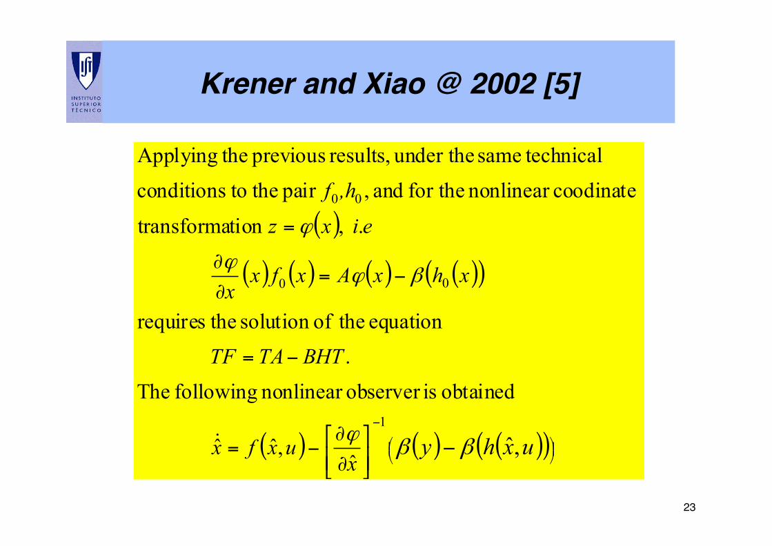
Krener and Xiao @ 2002 [5]!
( )
( ) ( ) ( ) ( )( )
( ) ( ) ( )( )⎟⎠⎞⎜⎝⎛
−
−⎥⎦⎤
⎢⎣⎡∂
∂−=
−=
−=∂
∂
=
uxhyx
uxfx
BHTTATF
xhxAxfxx
eixz
,hf
,ˆ1
00
00
ˆ,ˆˆ
obtained isobserver nonlinear following The.
equation theofsolution therequires
. ,tion transforma
coodinatenonlinear for the and ,pair the toconditions technicalsame under the results, previous theApplying
ββϕ
βϕϕ
ϕ
!
24!
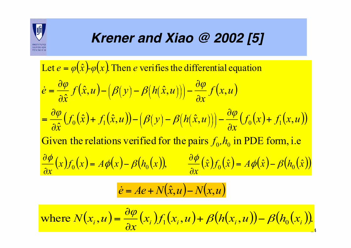
Krener and Xiao @ 2002 [5]!
( ) ( )
( ) ( )
( ) ( )( ) ( ) ( )( )
( ) ( ) ( ) ( )( ) ( ) ( ) ( ) ( )( )xhxAxfxx
xhxAxfxx
ex-φxφe
,hf
uxfxfxφuxhyuxfxf
xφ
uxfxφuxhyuxf
xφe
ˆˆˆˆ,
equation aldifferenti the verifiesThen .ˆLet
0000
00
1010
i.e form, PDEin pairs for the verifiedrelations Given the
,,ˆ,ˆˆˆ
,,ˆ,ˆˆ
βφ
βφ
φφ
ββ
ββ
−=∂
∂−=
∂
∂
=
+∂
∂−−−+
∂
∂=
∂
∂−−−
∂
∂=
⎟⎟⎠
⎞⎜⎜⎝
⎛⎟⎠⎞
⎜⎝⎛ ⎟
⎠⎞⎜
⎝⎛⎟
⎠⎞⎜
⎝⎛
⎟⎟⎠
⎞⎜⎜⎝
⎛⎟⎠⎞
⎜⎝⎛ ⎟
⎠⎞⎜
⎝⎛⎟
⎠⎞⎜
⎝⎛!
( ) ( )uxNuxNAee ,,ˆ −+=!
( ) ( ) ( ) ( )( ) ( )( ).,,, where 01 iiiii xhuxhuxfxxφuxN ββ −+∂
∂=
25!
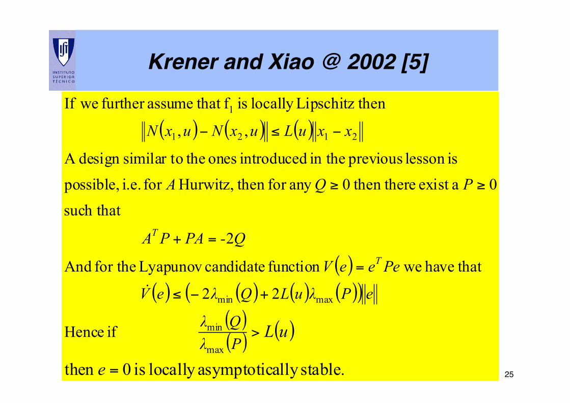
Krener and Xiao @ 2002 [5]!
( ) ( ) ( )
( )( ) ( ) ( ) ( )( )
( )( ) ( )
stable.ally asymptoticlocally is 0then max
min
maxmin
2121
1
if Hence
22
thathave wefunction candidate Lyapunov for the And
2
such that0 aexist e then ther0any for then Hurwitz, for i.e. possible,
islesson previous in the introduced ones thesimilar todesign A
,,
then Lipschitzlocally is f that assumefurther weIf
=
>
+−≤
=
=+
≥≥
−≤−
e
uLPλQλ
ePλuLQλeV
PeeeV
Q-PAPA
PQA
xxuLuxNuxN
T
T
!
26!
• Other methods to solve the PDE could be used [5]!
• Design method easier to be accomplished than [3]!
• The authors of [4] claim “to be able to do so for all linearly observable, real analytic systems whose spectrum of the linear part lies wholly in the right half complex plane”.!
• Krener and Xiao extended the method to arbitrary specta [5] (the Siegel domain) and showed that the sufficient conditions were also necessary.!
• Discrete time [6] and state and disturbance estimation design [7] versions became available!
Krener and Xiao @ 2002 [5]!
27!
References!
[1] !Mitter S., Baillieul J., and Willems J., “Mathematical Control Theory,” 1998.!!
[2] ! Kokotovic P. and Arcak M., “Constructive Nonlinear Control: A Historical Perspective,” Elsevier, 2000.!
!
[3] Krener A. and Isidori A. , “Linearization by Output Injection and Nonlinear Observers”, Systems and Control Letters, nº3, pp. 47-52, 1983.!
!
[4] Kazantzis N. and Kravaris C., “Nonlinear Observer Design using Lyapunov’s Auxiliary Theorem,” CDC, San Diego,1997. !
!
[5] ! Krener A. and Xiao M., “Nonlinear Observer Design in the Siegel Domain,” SIAM Journal of Control and Optimization, v. 41, nº 3, pp. 932-953, 2002. !
!
[6] Xiao M., Kazantzis N., Kravaris C., and Krener A., “Nonlinear Discrete-time Observer Design with Linearizable Error Dynamics,” IEEE Trans. Automatic Control, v.48, nº4, pp. 622-626, 2003. !
!
[7] !Kravaris C., Sotiropoulos V., Georgiou C., Kazantzis N., Xiao M., and Krener A., “Nonlinear Observer Design for State and Disturbance Estimation,” Systems and Control Letters, v. 57, pp. 730-735, 2007.!
!