September 2003 1

BASIC TECHNIQUES IN STATISTICAL NLP

Word predictionn-gramssmoothing

September 2003 2

Statistical Methods in NLE

Two characteristics of NL make it desirable to endow programs with the ability to LEARN from examples of past use:

– VARIETY (no programmer can really take into account all possibilities)

– AMBIGUITY (need to have ways of choosing between alternatives)

In a number of NLE applications, statistical methods are very common

The simplest application: WORD PREDICTION

September 2003 3

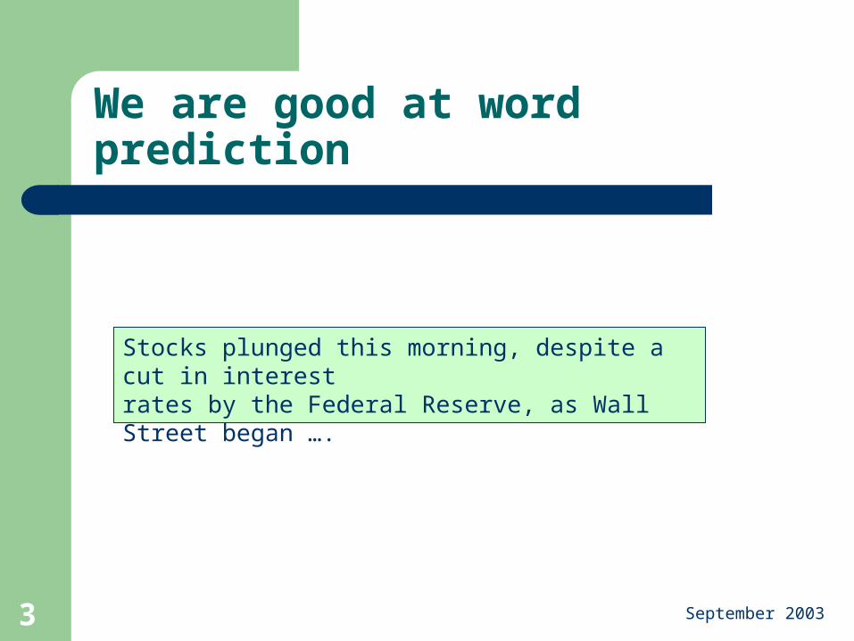
We are good at word prediction

Stocks plunged this morning, despite a cut in interestStocks plunged this morning, despite a cut in interestrates by the Federal Reserve, as WallStocks plunged this morning, despite a cut in interestrates by the Federal Reserve, as WallStreet began ….

September 2003 4

Real Spelling Errors

They are leaving in about fifteen minuets to go to her house

The study was conducted mainly be John Black.

The design an construction of the system will take more than one year.

Hopefully, all with continue smoothly in my absence.

Can they lave him my messages?

I need to notified the bank of this problem.

He is trying to fine out.

September 2003 5

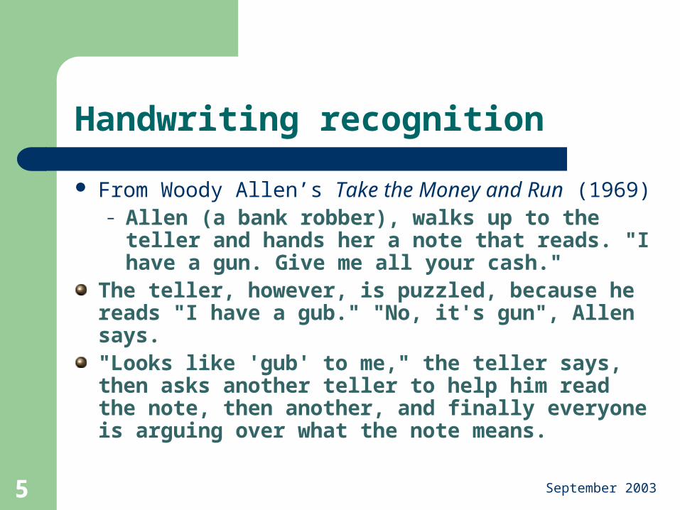
Handwriting recognition

From Woody Allen’s Take the Money and Run (1969)– Allen (a bank robber), walks up to the teller and

hands her a note that reads. "I have a gun. Give me all your cash."

The teller, however, is puzzled, because he reads "I have a gub." "No, it's gun", Allen says. "Looks like 'gub' to me," the teller says, then asks another teller to help him read the note, then another, and finally everyone is arguing over what the note means.

September 2003 6

Applications of word prediction

Spelling checkers Mobile phone texting Speech recognition Handwriting recognition Disabled users

September 2003 7

Statistics and word prediction

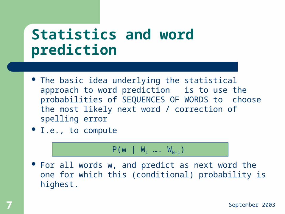
The basic idea underlying the statistical approach to word prediction is to use the probabilities of SEQUENCES OF WORDS to choose the most likely next word / correction of spelling error

I.e., to compute

For all words w, and predict as next word the one for which this (conditional) probability is highest.

P(w | W1 …. WN-1)

September 2003 8

Using corpora to estimate probabilities

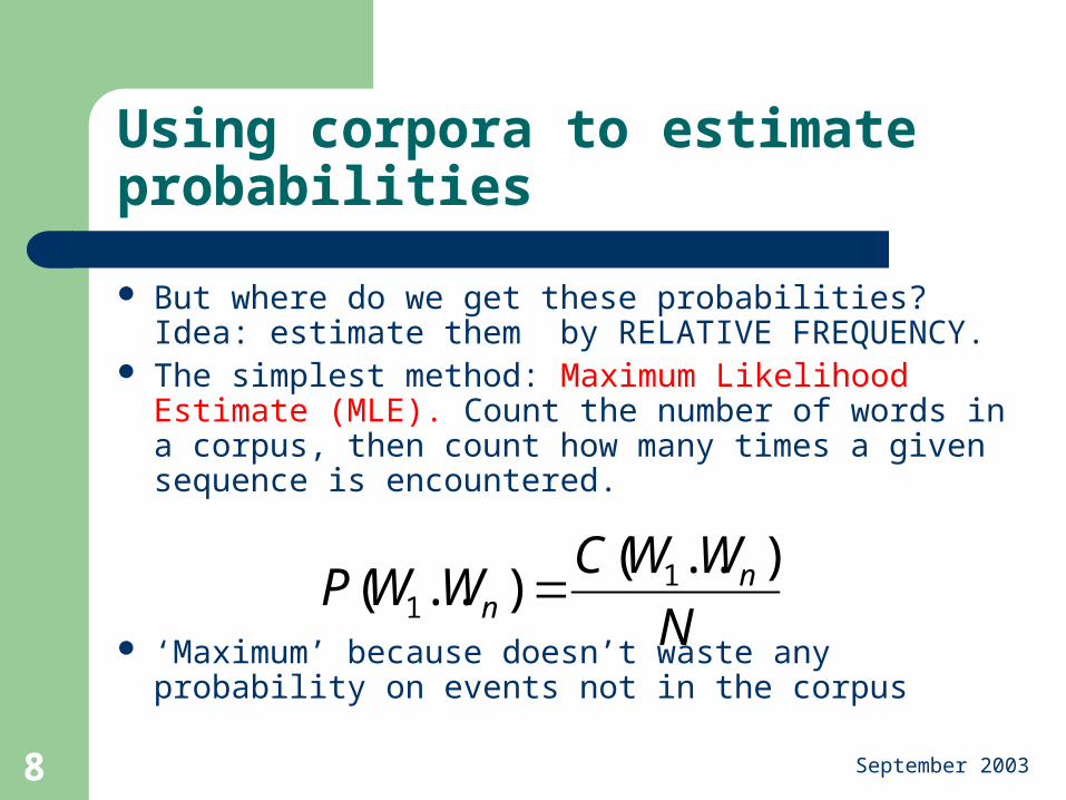
But where do we get these probabilities? Idea: estimate them by RELATIVE FREQUENCY.

The simplest method: Maximum Likelihood Estimate (MLE). Count the number of words in a corpus, then count how many times a given sequence is encountered.

‘Maximum’ because doesn’t waste any probability on events not in the corpus

N

WWCWWP nn

)..()..( 1

1

September 2003 9

Maximum Likelihood Estimation for conditional probabilities

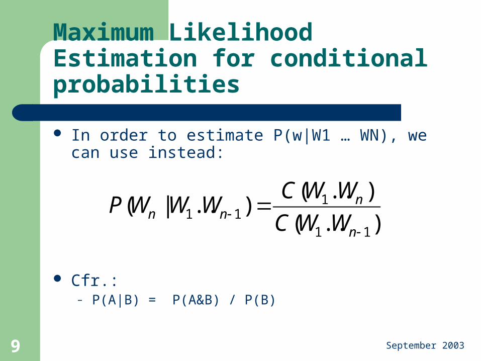
In order to estimate P(w|W1 … WN), we can use instead:

Cfr.: – P(A|B) = P(A&B) / P(B)

)..(

)..()..|(

11

111

n

nnn WWC

WWCWWWP

September 2003 10

Aside: counting words in corpora

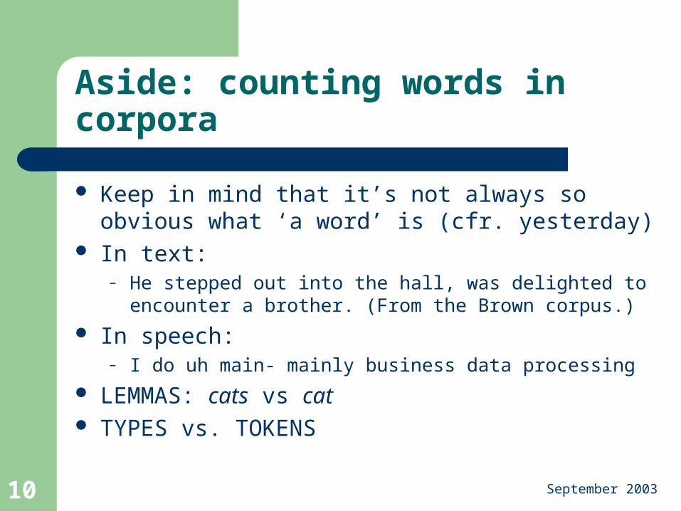
Keep in mind that it’s not always so obvious what ‘a word’ is (cfr. yesterday)

In text:– He stepped out into the hall, was delighted to encounter a

brother. (From the Brown corpus.)

In speech:– I do uh main- mainly business data processing

LEMMAS: cats vs cat TYPES vs. TOKENS

September 2003 11

The problem: sparse data

In principle, we would like the n of our models to be fairly large, to model ‘long distance’ dependencies such as:– Sue SWALLOWED the large green …

However, in practice, most events of encountering sequences of words of length greater than 3 hardly ever occur in our corpora! (See below)

(Part of the) Solution: we APPROXIMATE the probability of a word given all previous words

September 2003 12

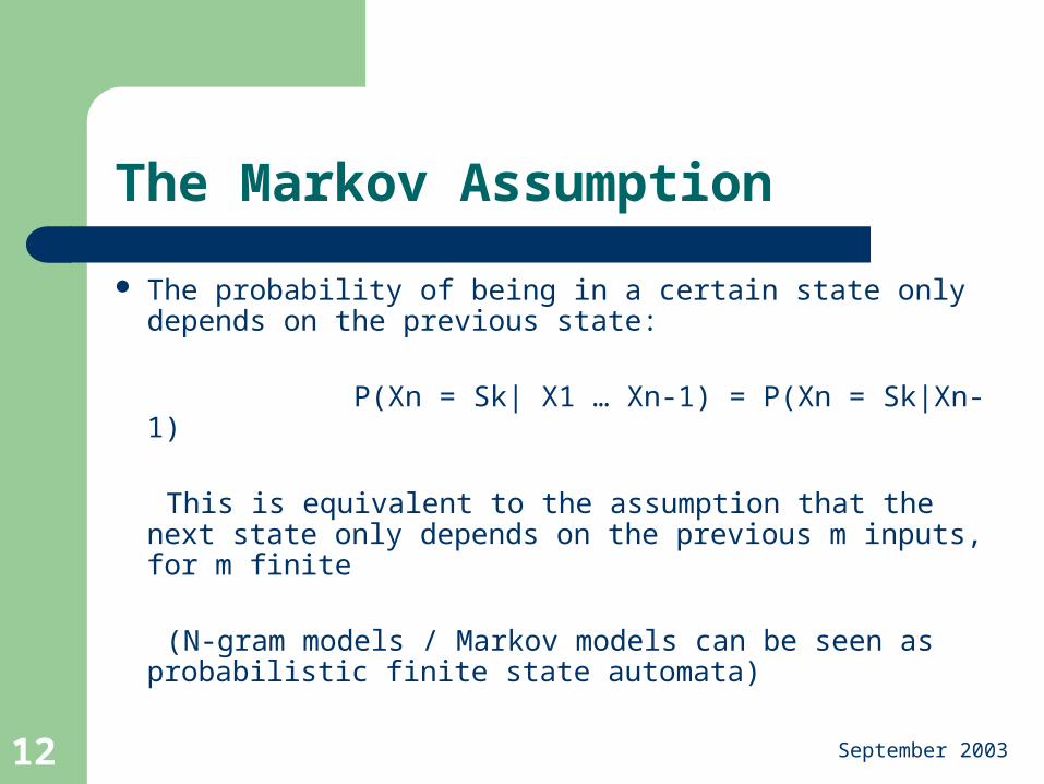
The Markov Assumption

The probability of being in a certain state only depends on the previous state:

P(Xn = Sk| X1 … Xn-1) = P(Xn = Sk|Xn-1)

This is equivalent to the assumption that the next state only depends on the previous m inputs, for m finite

(N-gram models / Markov models can be seen as probabilistic finite state automata)

September 2003 13

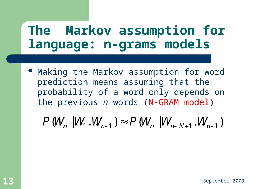
The Markov assumption for language: n-grams models

Making the Markov assumption for word prediction means assuming that the probability of a word only depends on the previous n words (N-GRAM model)

)..|()..|( 1111 nNnnnn WWWPWWWP

September 2003 14

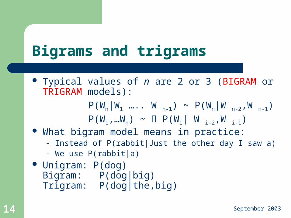
Bigrams and trigrams

Typical values of n are 2 or 3 (BIGRAM or TRIGRAM models):

P(Wn|W1 ….. W n-1) ~ P(Wn|W n-2,W n-1)

P(W1,…Wn) ~ П P(Wi| W i-2,W i-1) What bigram model means in practice:

– Instead of P(rabbit|Just the other day I saw a)– We use P(rabbit|a)

Unigram: P(dog)Bigram: P(dog|big)Trigram: P(dog|the,big)

September 2003 15

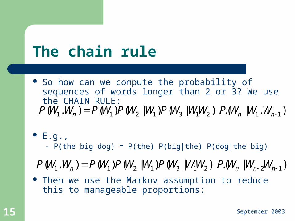
The chain rule

So how can we compute the probability of sequences of words longer than 2 or 3? We use the CHAIN RULE:

E.g., – P(the big dog) = P(the) P(big|the) P(dog|the big)

Then we use the Markov assumption to reduce this to manageable proportions:

)..|()..|()|()()..( 112131211 nnn WWWPWWWPWWPWPWWP

)|()..|()|()()..( 122131211 nnnn WWWPWWWPWWPWPWWP

September 2003 16

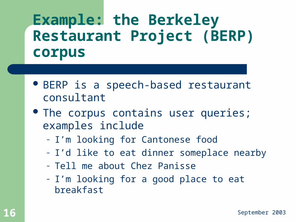
Example: the Berkeley Restaurant Project (BERP) corpus

BERP is a speech-based restaurant consultant The corpus contains user queries; examples

include– I’m looking for Cantonese food– I’d like to eat dinner someplace nearby– Tell me about Chez Panisse– I’m looking for a good place to eat breakfast

September 2003 17

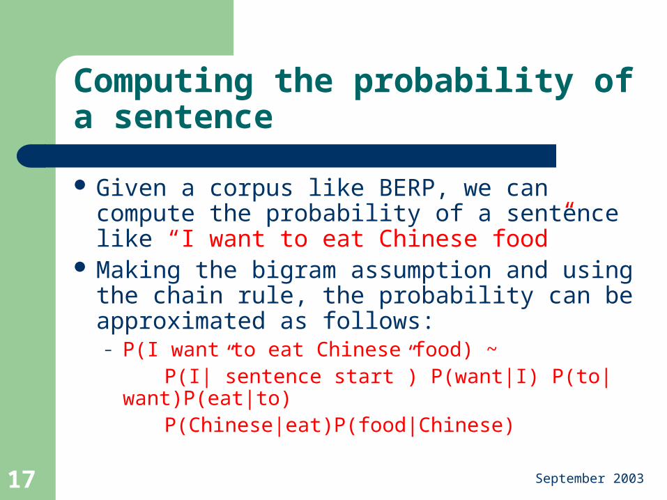
Computing the probability of a sentence

Given a corpus like BERP, we can compute the probability of a sentence like “I want to eat Chinese food”

Making the bigram assumption and using the chain rule, the probability can be approximated as follows:– P(I want to eat Chinese food) ~ P(I|”sentence start”) P(want|I) P(to|want)P(eat|to) P(Chinese|eat)P(food|Chinese)

September 2003 18

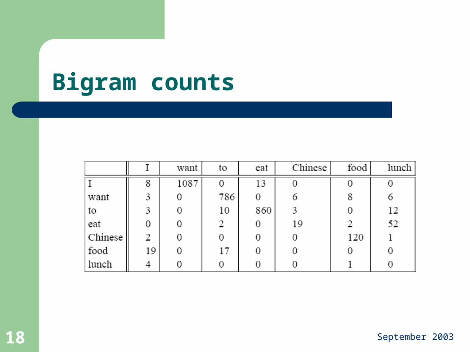
Bigram counts

September 2003 19

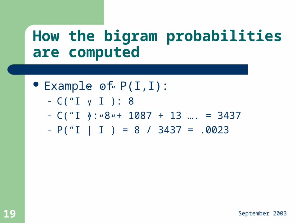
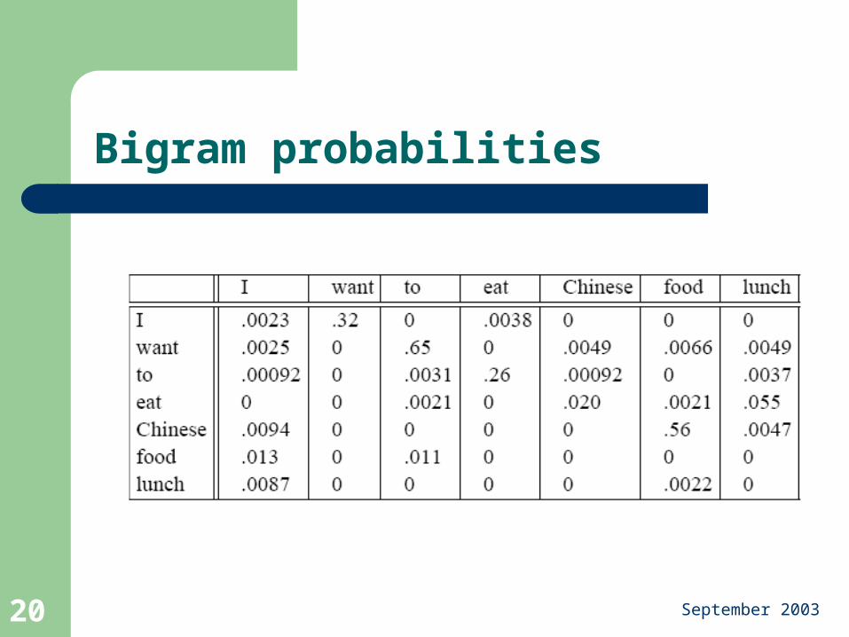
How the bigram probabilities are computed

Example of P(I,I):– C(“I”,”I”): 8– C(“I”): 8 + 1087 + 13 …. = 3437– P(“I”|”I”) = 8 / 3437 = .0023

September 2003 20

Bigram probabilities

September 2003 21

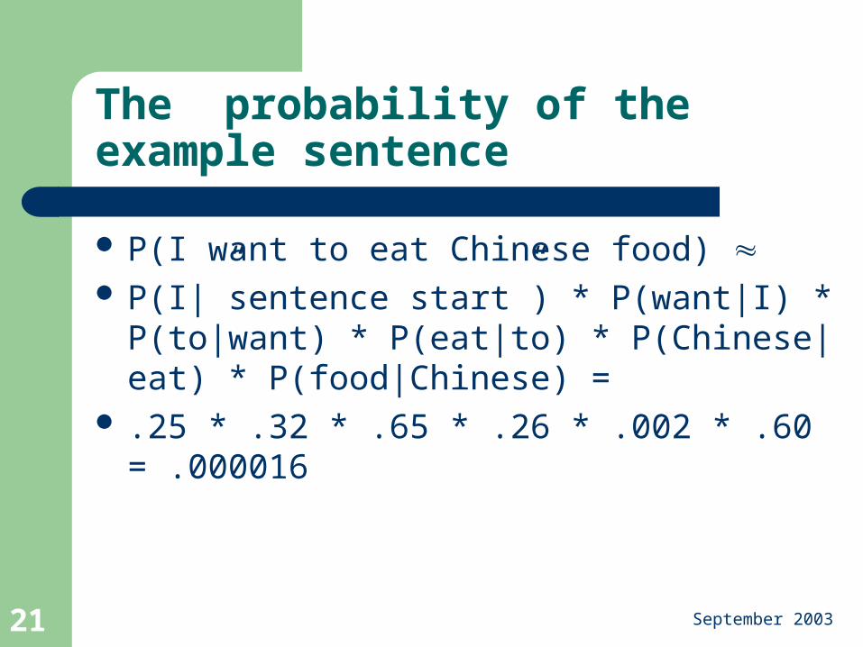
The probability of the example sentence

P(I want to eat Chinese food) P(I|”sentence start”) * P(want|I) * P(to|want) *

P(eat|to) * P(Chinese|eat) * P(food|Chinese) = .25 * .32 * .65 * .26 * .002 * .60 = .000016

September 2003 22

Examples of actual bigram probabilities computed using BERP

September 2003 23

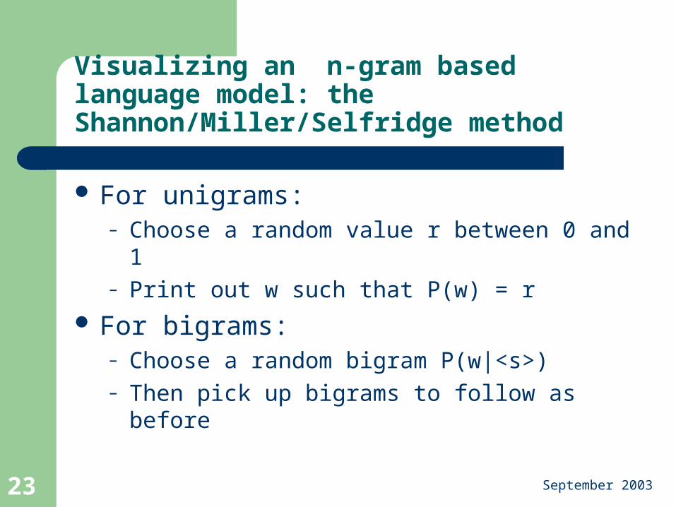
Visualizing an n-gram based language model: the Shannon/Miller/Selfridge method

For unigrams:– Choose a random value r between 0 and 1– Print out w such that P(w) = r

For bigrams:– Choose a random bigram P(w|<s>)– Then pick up bigrams to follow as before

September 2003 24

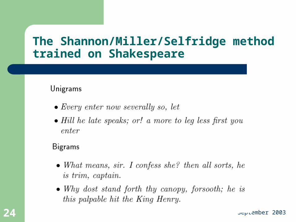
The Shannon/Miller/Selfridge method trained on Shakespeare

September 2003 25

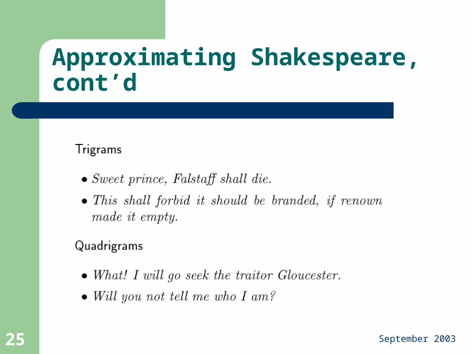
Approximating Shakespeare, cont’d

September 2003 26

A more formal evaluation mechanism

Entropy Cross-entropy

September 2003 27

The downside

The entire Shakespeare oeuvre consists of – 884,647 tokens (N)– 29,066 types (V)– 300,000 bigrams

All of Jane Austen’s novels (on Manning and Schuetze’s website): – N = 617,091 tokens– V = 14,585 types

September 2003 28

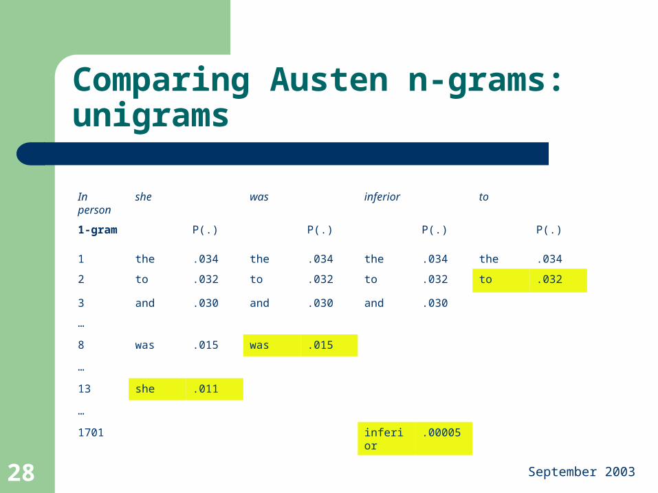
Comparing Austen n-grams: unigrams

In person

she was inferior to

1-gram P(.) P(.) P(.) P(.)

1 the .034 the .034 the .034 the .034

2 to .032 to .032 to .032 to .032

3 and .030 and .030 and .030

…

8 was .015 was .015

…

13 she .011

…

1701 inferior .00005

September 2003 29

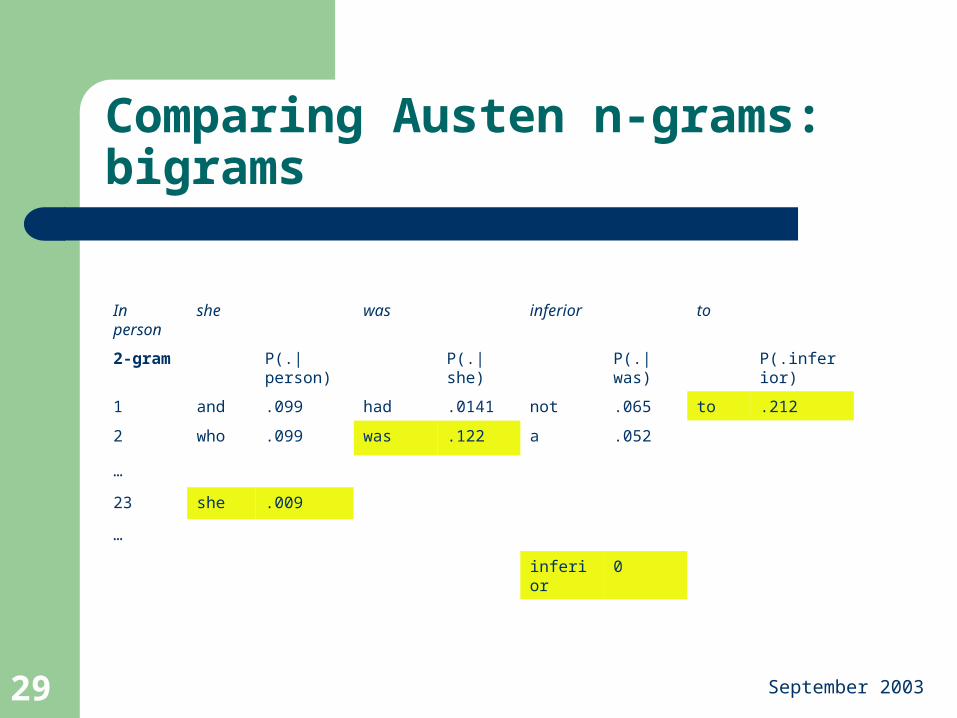
Comparing Austen n-grams: bigrams

In person

she was inferior to

2-gram P(.|person) P(.|she) P(.|was) P(.inferior)

1 and .099 had .0141 not .065 to .212

2 who .099 was .122 a .052

…

23 she .009

…

inferior 0

September 2003 30

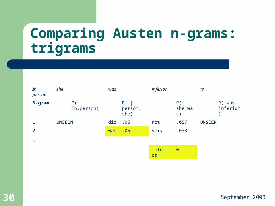
Comparing Austen n-grams: trigrams

In person

she was inferior to

3-gram P(.|In,person) P(.|person, she)

P(.|she,was)

P(.was,inferior)

1 UNSEEN did .05 not .057 UNSEEN

2 was .05 very .038

…

inferior 0

September 2003 31

Maybe with a larger corpus?

Words such as ‘ergativity’ unlikely to be found outside a corpus of linguistic articles

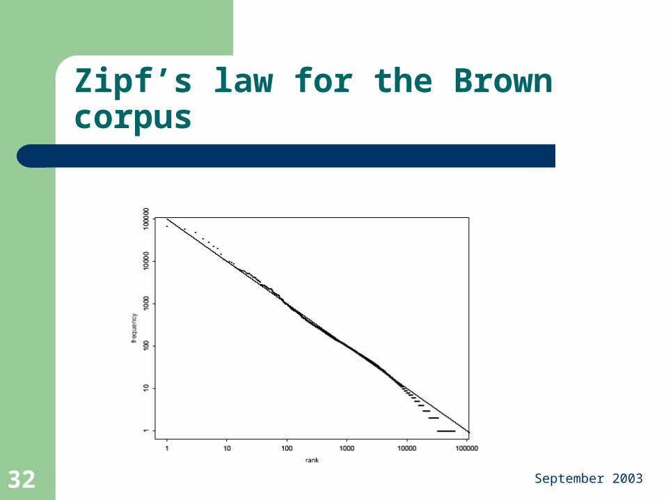
More in general: Zipf’s law

September 2003 32

Zipf’s law for the Brown corpus

September 2003 33

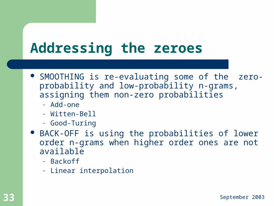
Addressing the zeroes

SMOOTHING is re-evaluating some of the zero-probability and low-probability n-grams, assigning them non-zero probabilities

– Add-one– Witten-Bell– Good-Turing

BACK-OFF is using the probabilities of lower order n-grams when higher order ones are not available

– Backoff– Linear interpolation

September 2003 34

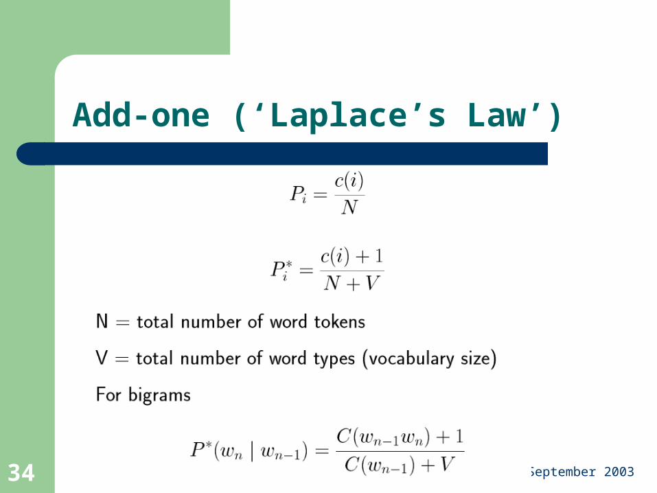
Add-one (‘Laplace’s Law’)

September 2003 35

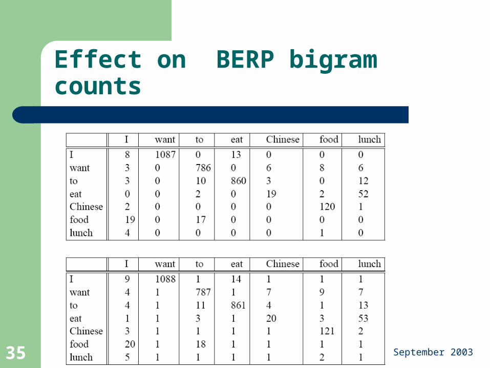
Effect on BERP bigram counts

September 2003 36

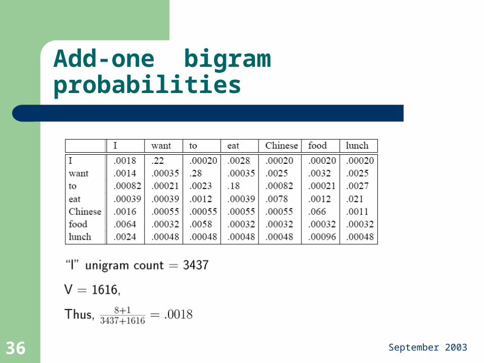
Add-one bigram probabilities

September 2003 37

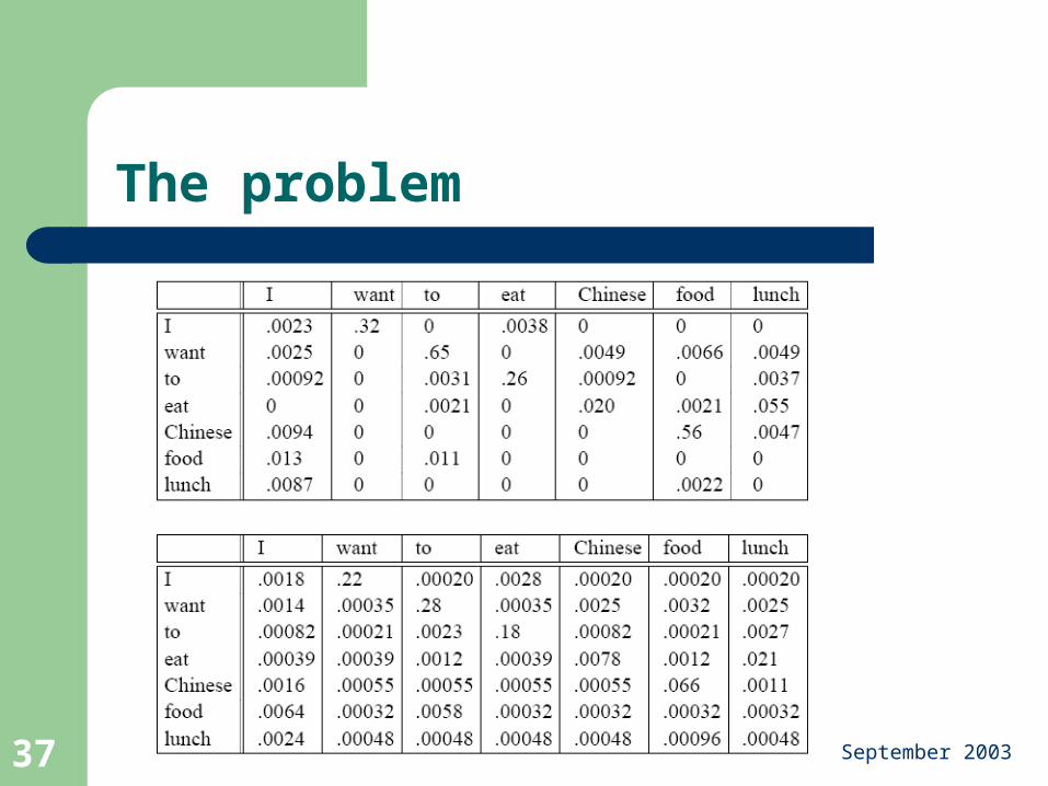
The problem

September 2003 38

The problem

Add-one has a huge effect on probabilities: e.g., P(to|want) went from .65 to .28!

Too much probability gets ‘removed’ from n-grams actually encountered– (more precisely: the ‘discount factor’

September 2003 39

Witten-Bell Discounting

How can we get a better estimate of the probabilities of things we haven’t seen?

The Witten-Bell algorithm is based on the idea that a zero-frequency N-gram is just an event that hasn’t happened yet

How often these events happen? We model this by the probability of seeing an N-gram for the first time (we just count the number of times we first encountered a type)

September 2003 40

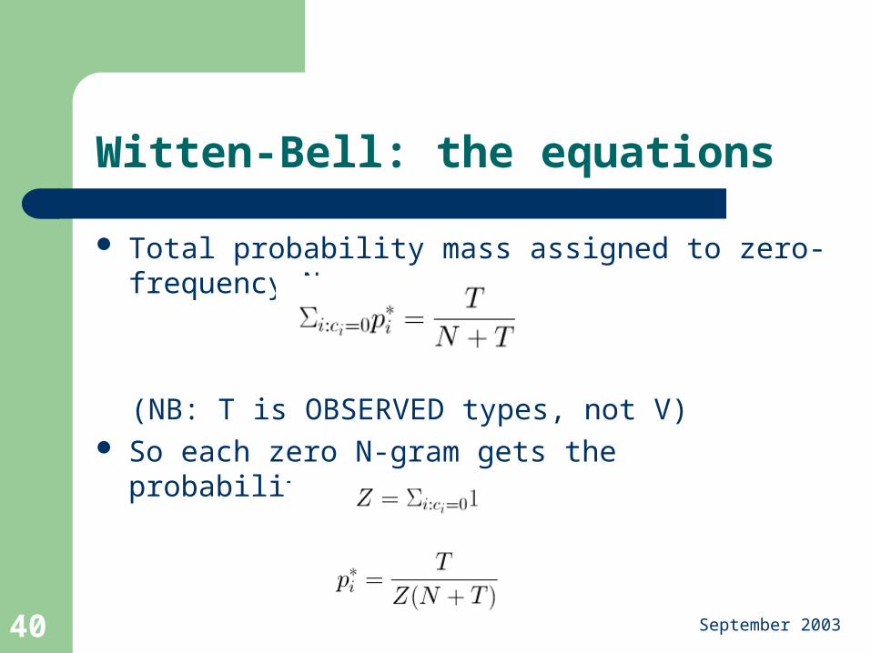
Witten-Bell: the equations

Total probability mass assigned to zero-frequency N-grams:

(NB: T is OBSERVED types, not V) So each zero N-gram gets the probability:

September 2003 41

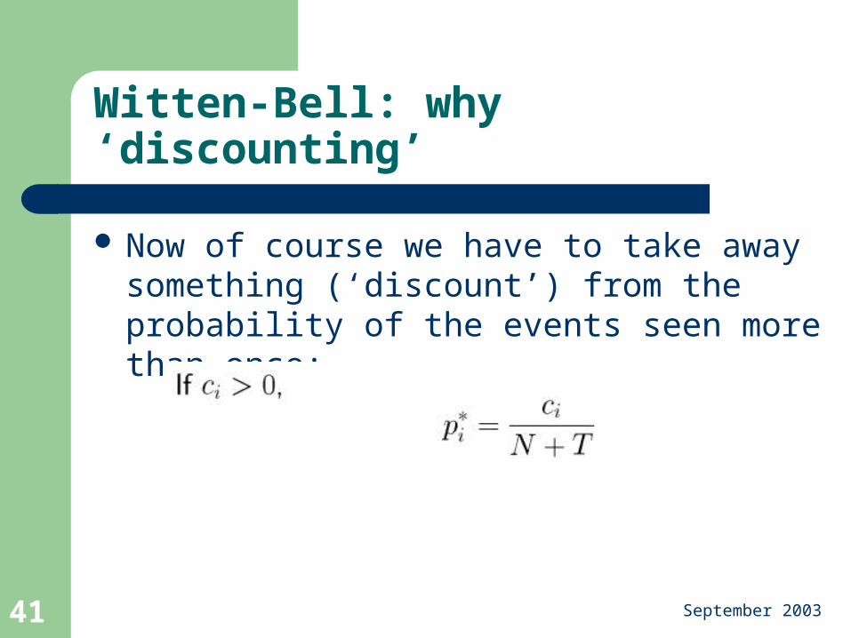
Witten-Bell: why ‘discounting’

Now of course we have to take away something (‘discount’) from the probability of the events seen more than once:

September 2003 42

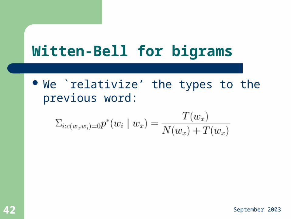
Witten-Bell for bigrams

We `relativize’ the types to the previous word:

September 2003 43

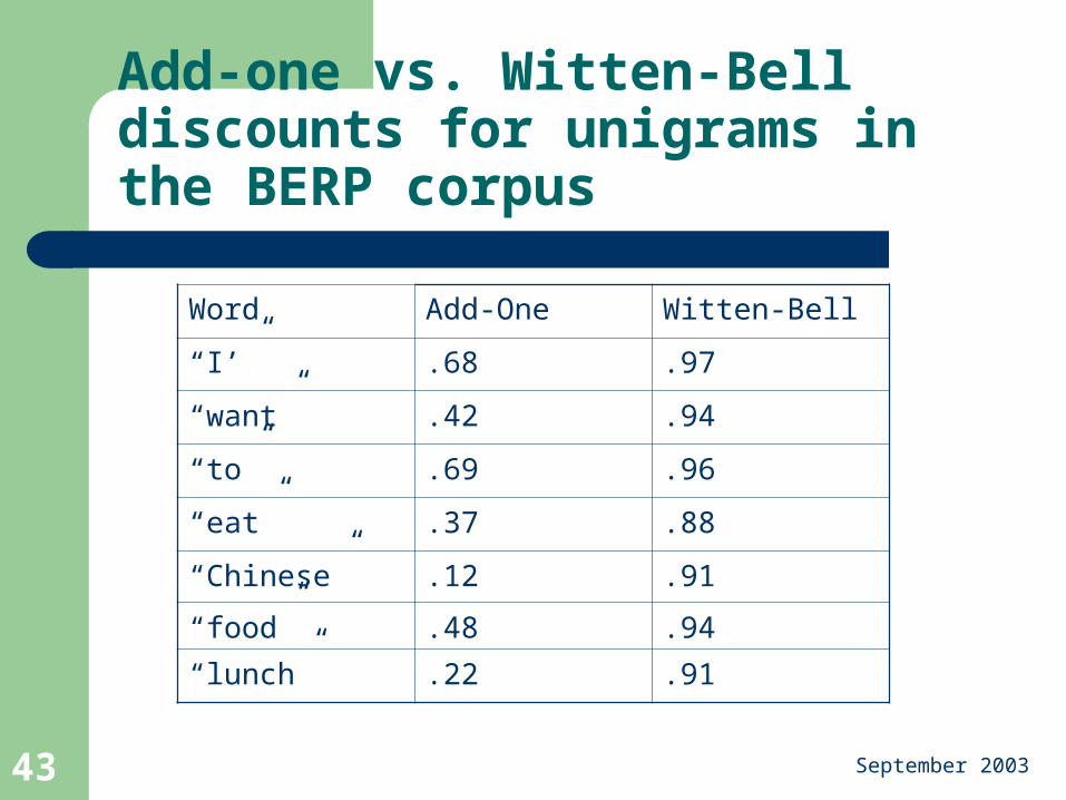
Add-one vs. Witten-Bell discounts for unigrams in the BERP corpus

Word Add-One Witten-Bell

“I’” .68 .97

“want” .42 .94

“to” .69 .96

“eat” .37 .88

“Chinese” .12 .91

“food” .48 .94

“lunch” .22 .91

September 2003 44

One last discounting method ….

The best-known discounting method is GOOD-TURING (Good, 1953)

Basic insight: re-estimate the probability of N-grams with zero counts by looking at the number of bigrams that occurred once

For example, the revised count for bigrams that never occurred is estimated by dividing N1, the number of bigrams that occurred once, by N0, the number of bigrams that never occurred

September 2003 45

Combining estimators

A method often used (generally in combination with discounting methods) is to use lower-order estimates to ‘help’ with higher-order ones

Backoff (Katz, 1987) Linear interpolation (Jelinek and Mercer, 1980)

September 2003 46

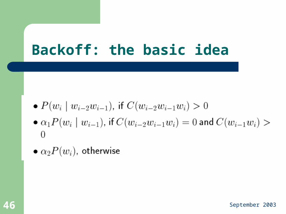
Backoff: the basic idea

September 2003 47

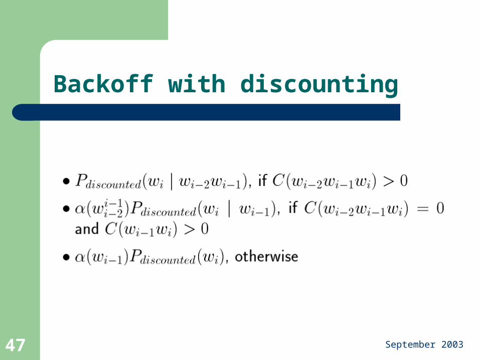
Backoff with discounting

September 2003 48

Readings

Jurafsky and Martin, chapter 6 The Statistics Glossary Word prediction:

– For mobile phones– For disabled users

Further reading: Manning and Schuetze, chapters 6 (Good-Turing)

September 2003 49

Acknowledgments

Some of the material in these slides was taken from lecture notes by Diane Litman & James Martin