Financial Economics Separation Theorem

Portfolio Choice with Many Risky Assets

Consider portfolio choice with many risky assets and a risk-free

asset. It turns out that the single risky asset model still applies!

1

Financial Economics Separation Theorem

Efficient Frontier for Risky Assets

Consider all possible portfolios of risky assets only. Theseportfolios determine all possible combinations of mean andstandard deviation. In (standard deviation, mean)-space,typically a parabola forms the boundary of these combinations.

The upper left boundary constitutes the efficient frontier for

risky assets. For any point on the frontier, there is someportfolio that achieves this combination of mean and standarddeviation, and no other portfolio can achieve either the samemean with a lower standard deviation, or a lower standarddeviation with the same mean. One refers to this portfolio asefficient.

2

Financial Economics Separation Theorem

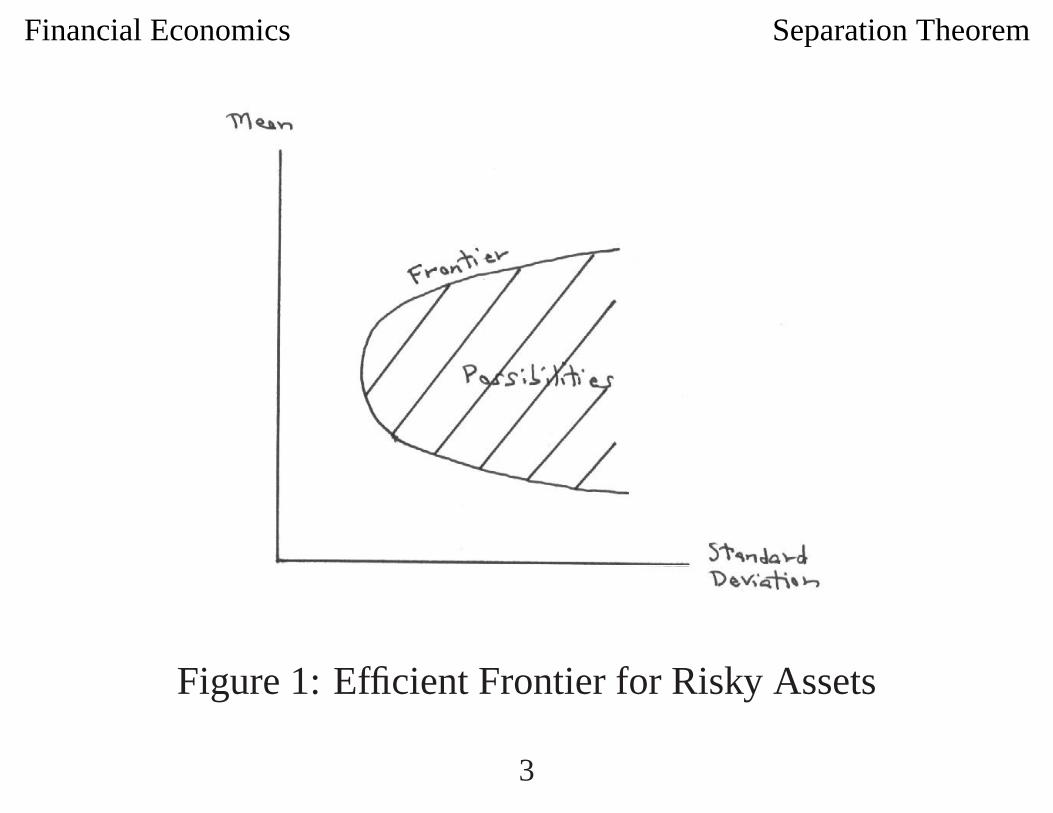
Figure 1: Efficient Frontier for Risky Assets

3

Financial Economics Separation Theorem

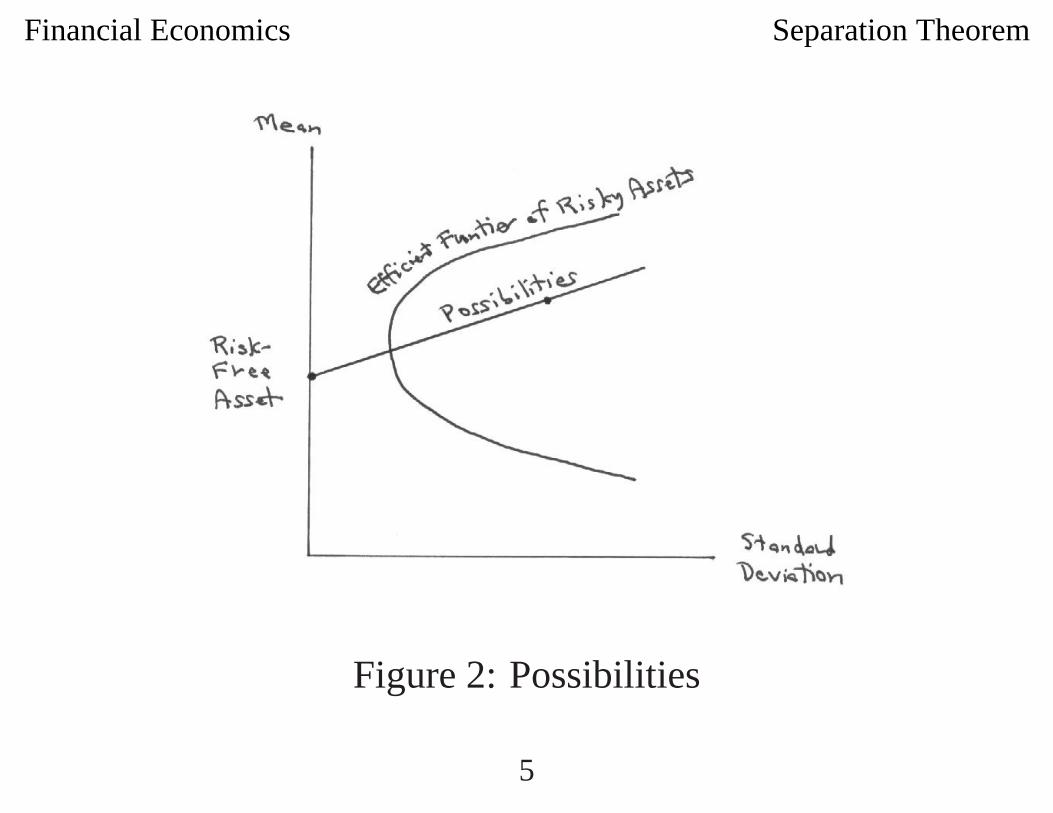
Risky Portfolio and Risk-Free Portfolio

Consider a portfolio in which one invests the fraction f of

wealth in a portfolio of risky assets and the fraction 1− f in the

risk-free asset. In (standard deviation, mean)-space, the

possible combinations lie along the straight line connecting the

(standard deviation, mean)-values for each.

4

Financial Economics Separation Theorem

Figure 2: Possibilities

5

Financial Economics Separation Theorem

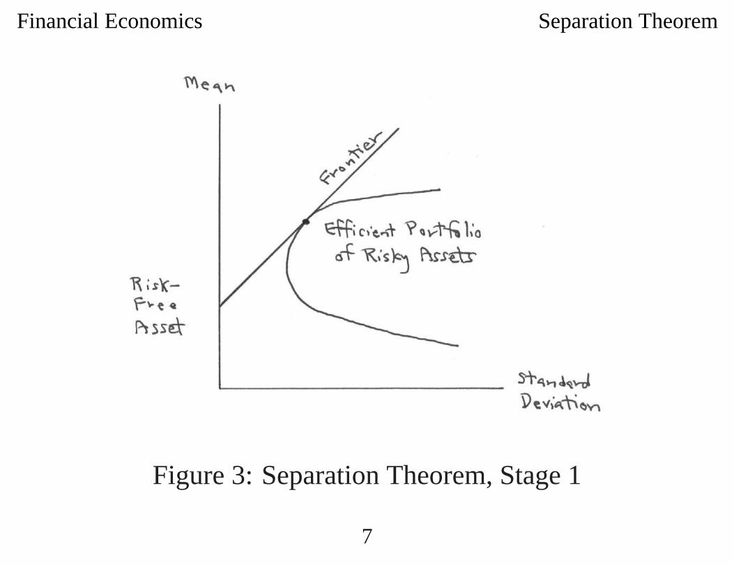
Efficient Frontier for All Assets

The efficient frontier for all assets is the line tangent to the

efficient frontier of risky assets passing though the point

(0, risk-free rate of return) for the risk-free asset.

Definition 1 (Efficient Portfolio of Risky Assets) The

efficient portfolio of risky assets is the portfolio corresponding

to the tangent point.

6

Financial Economics Separation Theorem

Figure 3: Separation Theorem, Stage 1

7

Financial Economics Separation Theorem

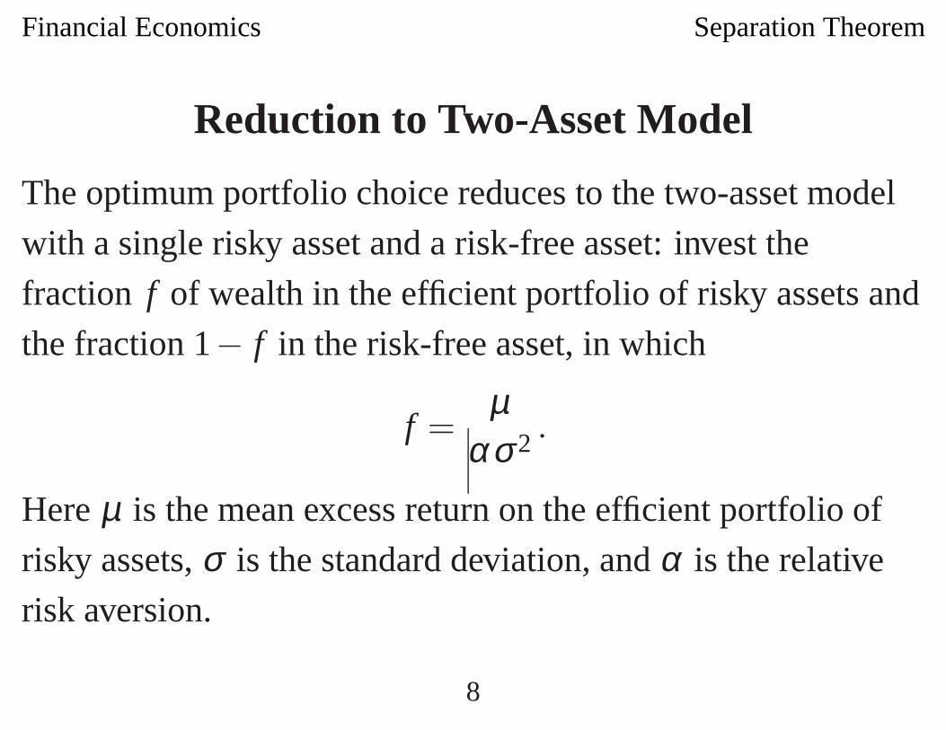
Reduction to Two-Asset Model

The optimum portfolio choice reduces to the two-asset model

with a single risky asset and a risk-free asset: invest the

fraction f of wealth in the efficient portfolio of risky assets and

the fraction 1− f in the risk-free asset, in which

f =µ

ασ 2 .

Here µ is the mean excess return on the efficient portfolio of

risky assets, σ is the standard deviation, and α is the relative

risk aversion.

8

Financial Economics Separation Theorem

Separation Theorem

Theorem 2 (Tobin [1]) Portfolio choice is separated into two

stages:

• Find the efficient portfolio of risky assets;

• Find the optimum fraction to invest in the efficient portfolio

of risky assets and the risk-free asset.

The role of risk aversion is confined to the second stage and

plays no role in the first stage.

9

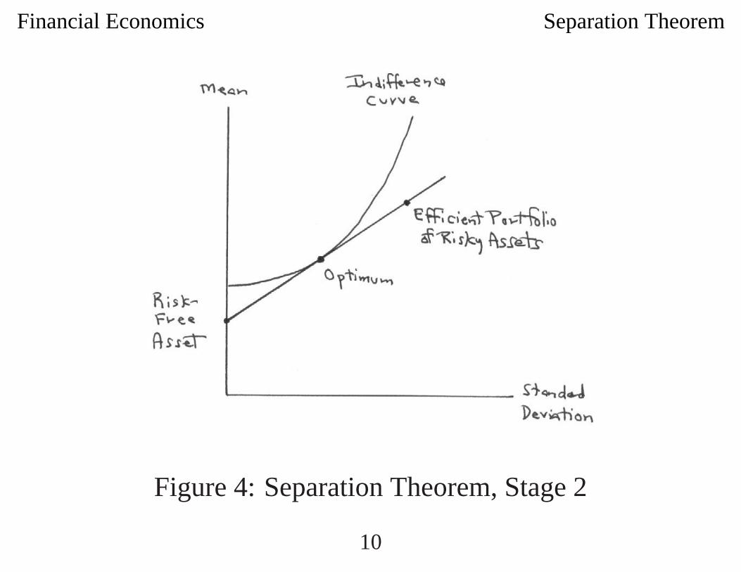
Financial Economics Separation Theorem

Figure 4: Separation Theorem, Stage 2

10

Financial Economics Separation Theorem

Tangent Slope

Suppose that m is the vector of mean excess returns on the

risky assets and that V is the variance (non-singular). Let fdenote a portfolio of risky assets, in which fi is the fraction of

wealth invested in asset i, normalized so

f�1 = 1 (1)

(1 is a vector with every component one).

11

Financial Economics Separation Theorem

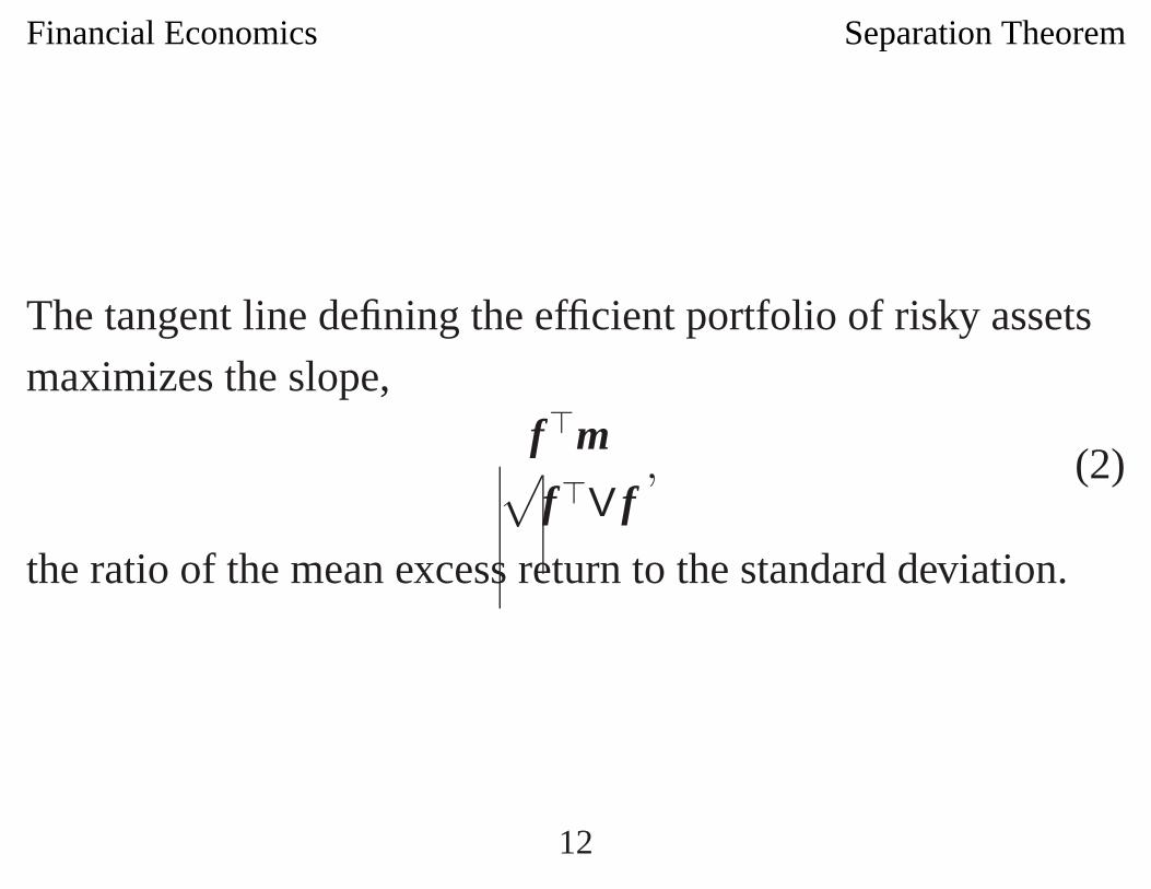
The tangent line defining the efficient portfolio of risky assets

maximizes the slope,f�m√f�V f

, (2)

the ratio of the mean excess return to the standard deviation.

12

Financial Economics Separation Theorem

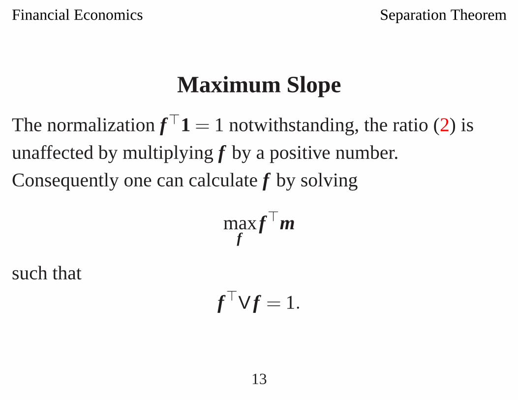
Maximum Slope

The normalization f�1 = 1 notwithstanding, the ratio (2) is

unaffected by multiplying f by a positive number.

Consequently one can calculate f by solving

maxf

f�m

such that

f�V f = 1.

13

Financial Economics Separation Theorem

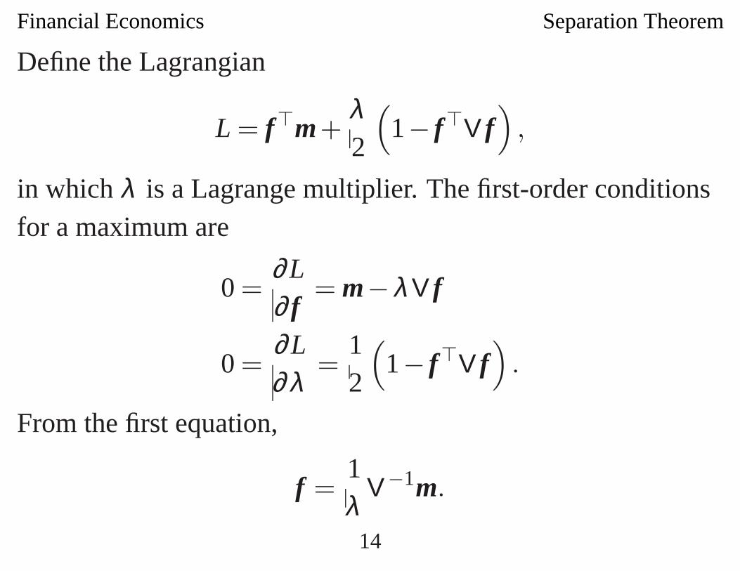
Define the Lagrangian

L = f�m+λ2

(1− f�V f

),

in which λ is a Lagrange multiplier. The first-order conditionsfor a maximum are

0 =∂L∂ f

= m−λ V f

0 =∂L∂λ

=12

(1− f�V f

).

From the first equation,

f =1λ

V−1m.

14

Financial Economics Separation Theorem

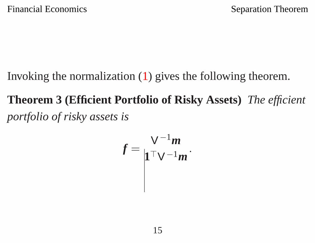
Invoking the normalization (1) gives the following theorem.

Theorem 3 (Efficient Portfolio of Risky Assets) The efficient

portfolio of risky assets is

f =V−1m

1�V−1m.

15

Financial Economics Separation Theorem

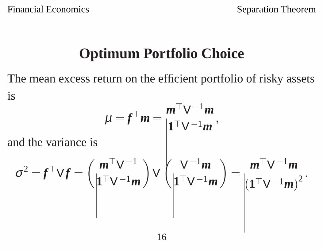
Optimum Portfolio Choice

The mean excess return on the efficient portfolio of risky assets

is

µ = f�m =m�V−1m1�V−1m

,

and the variance is

σ2 = f�V f =(

m�V−1

1�V−1m

)V

(V−1m

1�V−1m

)=

m�V−1m

(1�V−1m)2 .

16

Financial Economics Separation Theorem

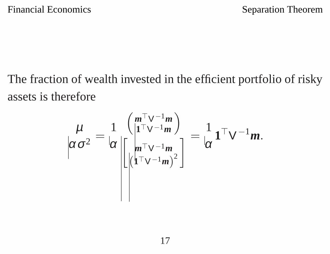
The fraction of wealth invested in the efficient portfolio of risky

assets is therefore

µασ 2 =

1α

(m�V−1m1�V−1m

)[

m�V−1m

(1�V−1m)2

] =1α

1�V−1m.

17

Financial Economics Separation Theorem

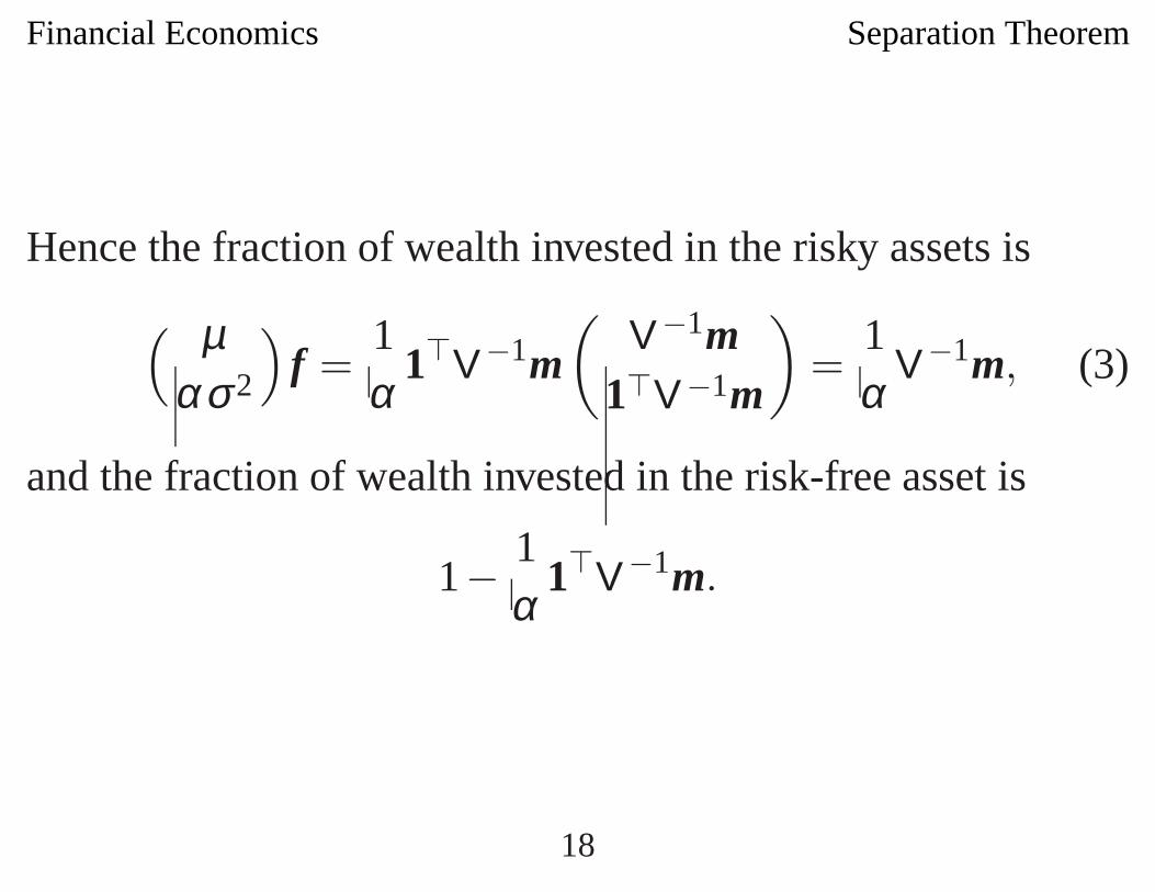
Hence the fraction of wealth invested in the risky assets is

( µασ 2

)f =

1α

1�V−1m(

V−1m1�V−1m

)=

1α

V−1m, (3)

and the fraction of wealth invested in the risk-free asset is

1− 1α

1�V−1m.

18

Financial Economics Separation Theorem

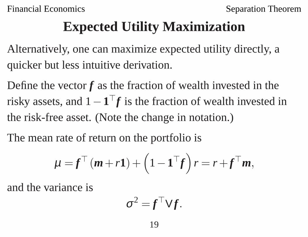
Expected Utility Maximization

Alternatively, one can maximize expected utility directly, aquicker but less intuitive derivation.

Define the vector f as the fraction of wealth invested in therisky assets, and 1−1�f is the fraction of wealth invested inthe risk-free asset. (Note the change in notation.)

The mean rate of return on the portfolio is

µ = f� (m+ r1)+(

1−1�f)

r = r + f�m,

and the variance is

σ2 = f�V f .

19

Financial Economics Separation Theorem

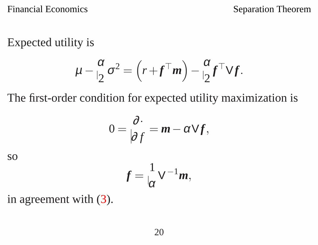
Expected utility is

µ − α2

σ2 =(

r + f�m)− α

2f�V f .

The first-order condition for expected utility maximization is

0 =∂ ·∂ f

= m−α V f ,

so

f =1α

V−1m,

in agreement with (3).

20

Financial Economics Separation Theorem

References

[1] James Tobin. Liquidity preference as behavior towards

risk. Review of Economic Studies, XXV(2):65–86,

February 1958. HB1R4.

21