Dynamic Point Coverage Problem in Wireless Sensor ...ceit.aut.ac.ir/~meybodi/paper/Esnaashari-2010-ad hoc and...One way to prolong the lifetime of a wireless sensor network is to schedule

“aswin150” — 2010/3/12 — 9:37 — page 193 — #1

Ad Hoc & Sensor Wireless Networks Vol. 10, pp. 193–234 ©2010 Old City Publishing, Inc.Reprints available directly from the publisher Published by license under the OCP Science imprint,Photocopying permitted by license only a member of the Old City Publishing Group

Dynamic Point Coverage Problem in WirelessSensor Networks: A Cellular Learning

Automata Approach

Mehdi Esnaashari and Mohammad Reza Meybodi

Soft Computing Laboratory, Computer Engineering and Information Technology Department,Amirkabir University of Technology, Tehran, Iran, P. O. Box: 15875-4413

E-mail: [email protected], [email protected]

Received: March 18, 2009. Accepted: September 14, 2009.

One way to prolong the lifetime of a wireless sensor network is to schedulethe active times of sensor nodes, so that a node is active only when it is reallyneeded. In the dynamic point coverage problem, which is to detect somemoving target points in the area of the sensor network, a node is needed tobe active only when a target point is in its sensing region. A node can beaware of such times using a predicting mechanism. In this paper, we pro-pose a solution to the problem of dynamic point coverage using irregularcellular learning automata. In this method, learning automaton residing ineach cell in cooperation with the learning automata residing in its neigh-boring cells predicts the existence of any target point in the vicinity of itscorresponding node in the network. This prediction is then used to sched-ule the active times of that node. In order to show the performance of theproposed method, computer experimentations have been conducted. Theresults show that the proposed method outperforms the existing methodssuch as LEACH, GAF, PEAS and PW in terms of energy consumption.

Keywords: Wireless Sensor Network, dynamic point coverage, scheduling, learningautomata, cellular learning automata.

1 INTRODUCTION

One important problem addressed in literature is the sensor coverage prob-lem. This problem is centered on a fundamental question: “How well do thesensors observe physical space?” The coverage concept is a measure of thequality of service (QoS) of the sensing function and is subject to a wide range

193

“aswin150” — 2010/3/12 — 9:37 — page 194 — #2

194 M. Esnaashari and M. Reza Meybodi

of interpretations due to a large variety of sensors and applications [88]. Var-ious coverage formulations have been proposed in literature among whichfollowing three are most discussed [1]:

• Area coverage: Covering (monitoring) the whole area of the network isthe main objective of area coverage problem.

• Point coverage: The objective of point coverage problem is to cover aset of stationary or moving target points using as little sensor nodes aspossible.

• Barrier coverage: Barrier coverage can be considered as the coveragewith the goal of minimizing the probability of undetected penetrationthrough the barrier (sensor network).

In this paper, we focus on the problem of dynamic point coverage whichis the point coverage problem with non-stationary target points. Any solutionto this problem must select a subset of sensor nodes in the network to beactive and monitor the target points. This can be done through a fixed or adynamic scheduling mechanism. In fixed scheduling mechanisms [2, 3, 5,39–43, 47–57], the set of sensors in the network is divided into disjoint setsso that every set completely covers the entire area of the network. Thesedisjoint sets are activated successively, so at any moment in time only oneset is active. Because all target points are monitored by every sensor set, thegoal of this approach is to determine a maximum number of disjoint sets sothat the time interval between two activations for any given sensor is longer.Besides its complexity, this approach needs the information of the networktopology to be available in a central node which is not always possible. Indynamic scheduling mechanisms, nodes are locally scheduled to be active orinactive based on the movement paths of target points [6–10, 11, 59–69]. Insuch schemes, usually some of the nodes which have higher residual energythan other nodes are active all of the times and monitoring the whole areafor detecting target points. Whenever a target point is detected, these activenodes track the target and estimate its movement path. This estimation leadsto a prediction about the location of the target point in near future. Sleepingnodes in the vicinity of the predicted location are then activated by currentlyactive nodes. This activation is performed using some sort of notificationmessages. This dynamic scheduling approach has two major drawbacks; oneis the overhead of the notification messages and the other is that sleeping nodesshould have the ability to receive messages, and hence they cannot power offtheir receiving antenna. This means that a sleeping node can only switch offits processing unit, but its communicating unit must be in idle state, waitingfor notification messages. According to [12], energy consumption of a sensornode in receiving and idle states is nearly equal to the energy consumed duringthe transmission state. As the energy consumed by a processing unit is in theorder of .001 of the energy consumed by a communicating unit, it is concluded

“aswin150” — 2010/3/12 — 9:37 — page 195 — #3

DPC Problem: A CLA Approach 195

that using these dynamic scheduling mechanisms, not so much energy savingcan be gained in sleeping nodes.

To overcome the above drawbacks, in this paper a novel dynamic schedul-ing algorithm based on irregular cellular learning automata is proposed todeal with the problem of dynamic point coverage. In the proposed algorithm,the sensor network is mapped into an irregular cellular learning automata.In this mapping, each sensor node in the network is mapped into a cell inthe ICLA. Each cell is equipped with a learning automaton. The learningautomaton residing in each cell in cooperation with the learning automataresiding in neighboring cells dynamically learns (predicts) the existence ofany target points in the vicinity of its corresponding node in the network innear future. This prediction is then used to schedule the active times of thatnode. Instead of notification messages which are exchanged between neigh-boring nodes in the dynamic scheduling schemes, in the proposed method, alocal base station in each neighborhood is always active and is responsiblefor queuing and relaying control packets between neighbor nodes during theiractive times. As a consequence, sleeping nodes in the proposed method canswitch off their communicating units as well as their processing units, sav-ing more energy and hence prolonging the network lifetime. Experimentalresults show that the proposed method outperforms the existing methods suchas LEACH1 [19], GAF2 [29], PEAS3 [55, 89] and PW4 [7] in terms of energyconsumption.

The rest of this paper is organized as follows. Section 2, gives a briefliterature overview. The problem statement is given in Section 3. Learningautomata, cellular learning automata and irregular cellular learning automatawill be discussed in Section 4. In Section 5 the proposed method is presented.Simulation results are given in Section 6. Section 7 is the conclusion.

2 RELATED WORK

We classify the scheduling algorithms into 3 categories; MAC layer algo-rithms, routing layer algorithms and application layer algorithms. Applicationlayer algorithms can be further classified into grid-based algorithms, coverage-related algorithms and tracking-based algorithms.

MAC Layer scheduling algorithms: In this category of algorithms,scheduling is performed in the MAC layer [21–28]. Usually, this is done byallocating a slot for one node per neighborhood uniquely. This collision-freeslot is used by that node for transmissions to any or all of its neighbors. Thus

1Low Energy Adaptive Clustering Hierarchy.2Geographical Adaptive Fidelity.3Probing Environment and Adaptive Sensing.4Proactive Wakeup based on PEAS.

“aswin150” — 2010/3/12 — 9:37 — page 196 — #4


two nodes cannot be assigned the same slot if one station is within the range ofthe others, or if two stations have common neighbors. The objective of thesealgorithms is to allow communication without interference, while maximizingthe number of parallel transmissions.

Routing layer scheduling algorithms: This category of scheduling algo-rithms relates to the hierarchical routing [14–20]. In hierarchical routingalgorithms, usually a number of clusters are formed in the network, each hav-ing one node as cluster head. The rest of the nodes in each cluster are calledcluster members. Cluster members must send their readings to their clusterheads, therefore, cluster heads schedule the sending time of their membersto prevent intra-cluster collisions. This way, a cluster member needs to beactivated only at its scheduled sending times.

One of the famous hierarchical routing layer algorithms is LEACH [19]given by Heinzelmanet al. In this algorithm, each node locally and basedon a random probability decides to be a cluster head. A cluster head thenadvertises itself in the area of the network. Other nodes join one of the clustersadvertised in the network based on the signal strength of the advertisementpackets. When clusters are formed, each cluster head adapts a TDMA-basedscheduling approach for data transmissions within its cluster. Each sensor nodesk in a cluster sends its reading to its cluster head at the time slots assignedto sk by the cluster head. Each cluster head receives data packets from itsmembers, aggregates them and sends them directly to the sink node.

Grid-based scheduling algorithms: In this category of scheduling algo-rithms [29–38], usually the network is partitioned into rectangular orhexagonal grids. Only one node is scheduled to be active in each grid atany time, to monitor that grid and to relay the data from other grids. Griddimensions are calculated in such a way that a node resides within a grid canmonitor the whole area of that grid and communicate with all nodes residingin its neighboring grids.

GAF [29] algorithm given by Xuet al. is one of the most known grid-basedalgorithms in the sensor network. In this algorithm, the area of the networkis partitioned into a number of rectangular cells. The dimensions of each cellis selected so that each node resides within a cell can monitor the entire areaof that cell and be able to communicate with any node resides in its adjacentcells. Each nodesk in a cell waits for a random duration to receive a packetfrom its neighbors within the same cell indicating that the sender of the packetwill be active in the cell. If no such packet is received,sk decides to becomethe active node of the cell and broadcasts a packet within its cell to indicateits decision. This packet also contains the active duration of the nodesk. Thisactive duration is selected based on the energy level ofsk; more energy levelresults in longer active duration. When the active node for each cell is selected,rest of the nodes in that cell will go to sleep for the duration of the specifiedactive duration. Selection of the active node for each cell is repeated when theactive duration of the active node of that cell is over.

“aswin150” — 2010/3/12 — 9:37 — page 197 — #5


Coverage-related scheduling algorithms: This category of schedulingalgorithms, deals with the problem of covering (monitoring) either the entirearea of the network or some target points (stationary or moving) in the area ofthe network using as little sensor nodes as possible [1]. Usually, a minimumnumber of nodes are selected to be active and monitor the area or the targetpoints while the rest of the nodes are inactive and save energy. The node selec-tion is repeated periodically or based on a certain schedule to allow balanceenergy consumption of all nodes. A number of centralized [2–4, 39–43] anddecentralized [5, 15, 42–58] methods are given in literature for addressingthis problem. In centralized methods, by assuming that the sink node has thetopology information of the network, usually the problem is solved optimallyusing a linear integer programming approach or sub-optimally using a heuris-tic approach. In distributed methods, each node locally checks whether it isnecessary for it to be active or not. It is necessary for a node to be active only ifthe sensing region of the node cannot be covered completely by its neighbors.

One of the famous algorithms in this category is PEAS [55, 89] given byYe et al. At the startup of the algorithm, each nodesk sleeps for an exponen-tially distributed duration. When this duration is over,sk becomes active andprobes for an active node in its neighborhood. If some nodes are active inthe neighborhood of the node,sk returns to sleep mode for a newly selectedduration. This duration is computed based on the local information collectedduring the probing process. Otherwisesk stays in active mode until its energyis depleted completely.

Tracking-based scheduling algorithms: The last category of schedulingalgorithms is tracking-based algorithms. These scheduling algorithms are usedto address the tracking problem in which a number of targets are movingthroughout the network and the objective of the network is to monitor themovement path of these targets. Since at any instance of time, only a fractionof the nodes are able to monitor a moving target, the rest of the nodes can beinactive and save their energy. In these algorithms [6–10, 11, 59–69], usuallythe nodes which are currently monitoring the targets use some sort of predictionto predict the movement path of the targets. Based on this prediction, a subsetof currently inactive nodes which are more probable to be able to monitorthe moving targets in near future are scheduled to be activated. Activation isperformed using some sort of notification messages. Note that these methodsassume that inactive nodes have the ability to receive notification messages.

PW [7] given by Guiet al. is one of the most known tracking-basedscheduling algorithms given in literature. In this algorithm, the operationof the network is divided into two phases; surveillance and tracking. In thesurveillance phase, the network actively monitors the area to check if anytarget point enters the field. In the tracking phase, a target which has beenentered the field is being tracked by the network. In the surveillance phase, anextension of the PEAS algorithm called PECAS is used. The major differencebetween the PECAS and PEAS is in that an active node in PECAS algorithm

“aswin150” — 2010/3/12 — 9:37 — page 198 — #6


remains active only for a specified duration whereas in PEAS, an active noderemains active until its energy is completely depleted. In the tracking phase,each sensor node has four working modes: Waiting, Prepare, SubTrack, andTracking mode. Anode is in Tracking working mode if it is within a circle cen-tered around the location of the target with radiusr (tracking circle). A nodeis in SubTrack working mode if it is outside thetracking circle but within acircle centered around the location of the target with radiusr + R (subtrackcircle). A node is in Prepare working mode if it is outside thesubtrack circle,but within a circle centered around the location of the target with radiusr+2R(prepare circle). Rests of the nodes are in Waiting working mode. A node maychange its working mode if it senses a target, if it cannot sense a target anymore or if it receives a packet from a neighborsk indicating that a target existsin the sensing range ofsk.

3 PROBLEM STATEMENT

Consider a sensor network consists ofN sensor nodess1, s2, . . . , sN ,M reporter nodesr1, r2, . . . , rM and one sink within aL × L rectangular,completely known and accessible field (�). Sensor nodes, which are respon-sible for sensing and monitoring the field, are scattered randomly throughoutthe area of the network so that� is completely covered. Reporter nodes areplaced manually in specified positions within� and form an infrastructurethrough which packets received from sensor nodes are relayed towards thesink. This manual placement of reporter nodes is feasible since we assumethat� is completely known and accessible. Reporter nodes are powerful andrechargeable nodes which are always active. All sensor nodes have the samesensing range ofRs and communicating range ofRc. Each sensor nodesk has4 different modes of operation [72] as follows:

• On-duty (CPUASACA): CPU, sensing and communicating units areswitched on referred to as active mode.

• Sensing Unit On-duty (CPUASACS): The CPU and the sensing unitsare switched on, but the communicating unit is switched off.

• Communicating Unit On-duty (CPUASSCA): The CPU and the com-municating units are switched on, but the sensing unit is switchedoff.

• Off-duty (CPUSSSCS): CPU, sensing and communicating units areswitched off referred to as sleep mode.

Note that inCPUASACA, CPUASACS , CPUASSCA andCPUSSSCS , indexA stands for active and indexS stands for sleep. For further simplicity innotation, we use indexx in the above notations to refer to more than one

“aswin150” — 2010/3/12 — 9:37 — page 199 — #7


operation mode, i.e.CPUASACx refers to bothCPUASACA andCPUASACSmodes, andCPUxSxCx refers to all 4 modes of operation. At any instance oftime, a sensor node can be only in one of the above 4 operation modes. Theoperation mode of a sensorsk at time instantt is denoted byOsk (t).

Let P be a finite set of target points residing in�. P is divided into twodisjoint sets;Moving objects (PM ) andEvents (PE). A target pointpMi ∈ PMis a moving object which has a continuous movement trajectory. On the otherhand, a target pointpEi ∈ PE is an event which occurs somewhere in�repeatedly or randomly following a Poisson distribution and lasts for a shortstatic or random duration.

We denote the Euclidean distance between a sensor nodesk located at(x(sk), y(sk)) and a target pointpi located at(x(pk), y(pk)) asd(sk, pi), i.e.d(sk, pi) = √

(x(sk)− x(pi))2 + (y(sk)− y(pi))2.Assuming the binary sensing model [13] and sensing range ofRs for all

sensor nodes in the network, we say a target pointpi ∈ P is sensed, detectedor monitored by a sensor nodesk at timet if and only if d(sk, pi) < Rs andOsk (t) = CPUASACx . The network detects a target pointpi ∈ P at timet ifand only if at least one of the sensor nodes of the network detectspi at timet .

Definition 1. Network lifetime (T) is defined as the time elapsed from thenetwork startup to the time at which the� is not further completely coveredby the network due to node deaths.

Definition 2. Activation time of a target pointpi ∈ P denoted byτpi is thesummation of all the times during whichpi can be detected by the network.

Definition 3. Activation time of a sensor nodesk denoted byτsk is the sum-mation of all the times during which the sensor is inCPUASACx operationmode; that is Osk (t) = CPUASACx .

Definition 4. Detection time of a target pointpi ∈ P denoted byτdpi is thesummation of all the times during whichpi is detected by the network.

Definition 5. Detection time of a target pointpi ∈ P by a sensor nodeskdenoted byτsk,pi is the summation of all the times during whichpi is detectedby sk.

Definition 6. Network detection rate denoted byηD is the rate of the targetdetection in the network and is defined according to equation (1).

ηD =∑pi∈P τ

dpi∑

pi∈P τpi(1)

Definition 7. Network sleep rate denoted byηS is defined as the ratio of thetimes during which nodes of the network are in sleep mode to the times during

“aswin150” — 2010/3/12 — 9:37 — page 200 — #8


which they can be in sleep mode.ηS is defined according to equation (2).

ηS =∑sk

(T−τsk

T−∑pi∈P τsk ,pi

)N

(2)

The objective of the network is to detect the target points and report theirlocations to the sink. We assume that the reporter nodes are placed so that eachsensor node can directly communicate with at least oneri . Sensor nodes sendtheir packets directly to reporter nodes and reporter nodes forward receivedpackets towards the sink.

To prolong the network lifetime, a sensor node will switch to theCPUASxCA operation mode only if it wants to communicate with a reporternode; otherwise, the communicating unit of the sensor node will be switchedoff. The sensing unit of a sensor node has to be switched on only if a tar-get point is in its sensing range, but since sensor nodes have no knowledgeabout the movement paths of target points, they cannot calculate the timesfor switching their sensing units on or off. As an alternative way, we assumethe time to be divided into a number of very short epochs (Ep) having equaldurations (τEp). The sensing units of sensor nodes can be switched on or offonly at the startup of each epoch. Therefore, at the startup of each epochEpnk ,a sensor nodesk has to predict if any target points will pass through its sensingregion duringEpnk . Based on this prediction,sk switches its sensing unit onor off duringEpnk . Indexk in Epnk states that we assume no synchronizationbetween sensor nodes, and hence, each sensor node has its own timing andepochs. We refer to the operation mode of a sensor nodesk during the epochEpnk as Osk (Epnk).

Having the above definitions and assumptions, the problem is to locallypredict the status of the sensing unit of each node at the startup of each epochsuch that the network sleep rate (ηS) is maximized while the network detectionrate (ηD) does not drop below an acceptable level.

To clarify the problem, we give an application. A trial wireless sensornetwork which is going to be tested in San Francisco is a sensor networkthat announce which of the parking spaces of the city are free at any moment[70]. This network uses a wireless sensor embedded in a 4-inch-by-4-inchpiece of plastic, fastened to the pavement adjacent to each parking space.In this application, each sensor node has to monitor its parking space andreports the free times of the parking space to a local base station (a reporternode). The local base station then prepares the information of free parkingspaces for drivers passing the area and requesting such information. Fromthe viewpoint of the sensor network, cars coming into the parking spaces andgetting out of them are moving target points which must be monitored. If asensor nodesk switches periodically betweenCPUASACx andCPUxSSCxoperation modes, it will have a longer lifetime than if it always remains inCPUASACx operation mode, however this makes it possible for a driver to be

“aswin150” — 2010/3/12 — 9:37 — page 201 — #9


mistakenly guided tosk ’s parking space, while it is occupied by another car.Such incorrect guidances are acceptable while their rate is below an acceptablelevel, and hence, a local prediction can be performed in each sensor node topredict the status of its sensing unit at the startup of each epoch.

4 CELLULAR LEARNING AUTOMATA

In this section we briefly review cellular automata, learning automata, cellularlearning automata and irregular cellular learning automata.

Cellular Automata: Cellular automata (CA) is a mathematical model forsystems consisting of large number of simple identical components with localinteractions. CA is a non-linear dynamical system in which space and timeare discrete. It is called cellular because it is made up of cells like points ina lattice or like squares of checker boards, and it is called automata becauseit follows a simple rule [74]. CA performs complex computations with a highdegree of efficiency and robustness. Informally, a d-dimensional CA consistsof an infinite d-dimensional lattice of identical cells. Each cell can assumea state from a finite set of states. The state of each cell at any time instantis determined by a rule from states of neighboring cells at the previous timeinstant.

Learning Automata: Learning automata (LA) is an abstract model whichrandomly selects one action out of its finite set of actions and performs it ona random environment. Environment then evaluates the selected action andresponses to the automata with a reinforcement signal. Based on the selectedaction, and received signal, the automata updates its internal state and selectsits next action. Learning automata are classified into fixed-structure stochas-tic, and variable-structure stochastic. A variable-structure learning automatonis defined by the quadruple{α, β, p, T } in which α = {α1, α2, . . . , αr} rep-resents the action set of the automata,β = {β1, β2, . . . , βr} represents theinput set,p = {p1, p2, . . . , pr} represents the action probability set, andfinally p(n + 1) = T [α(n), β(n), p(n)] represents the learning algorithm.This automaton operates as follows. Based on the action probability setp,automaton randomly selects an actionαi , and performs it on the environment.After receiving the environment’s reinforcement signal, automaton updatesits action probability set based on equations (3) for favorable responses, andequations (4) for unfavorable ones.

pn+1i = pni + a.(1 − pni )

pn+1j = pnj − a.pnj ∀j j �= i

(3)

pn+1i = (1 − b).pni

pn+1j = b

r − 1+ (1 − b)pnj ∀j j �= i

(4)

“aswin150” — 2010/3/12 — 9:37 — page 202 — #10


In these equations,a andb are reward and penalty parameters respectively. Ifa = b, learning algorithm is calledLR−P 5, if b � a, it is calledLRεP 6, andif b = 0, it is calledLR−I 7. For more information about learning automatathe reader may refer to [75, 76].

Cellular Learning Automata: Cellular learning automata, which is a combi-nation of cellular automata and learning automata, is a powerful mathematicalmodel for many decentralized problems and phenomena. A CLA is a CA inwhich a learning automaton is assigned to every cell. At any instant of time,the action probability vector of the LA resides in a particular cell constitutesthe state of that cell. Like CA, there is a rule that the CLA operates under.The local rule of CLA and the actions selected by the neighboring LAs of anyparticular LA determine the reinforcement signal to that LA. The neighboringLAs of any particular LA constitute the local environment of the cell in whichthat LA resides. The local environment of a cell is nonstationary because theaction probability vectors of the neighboring LAs vary during the evolutionof the CLA. The operation of a CLA could be described as follows: At thefirst step, the internal state of every cell is specified. This initial value maybe chosen on the basis of past experience or at random. In the second step,each LA selects one of its actions based on its action probability vector andperforms it on the environment. Next, the local rule of CLA determines thereinforcement signal to each LA. Finally, each LA updates its action proba-bility vector on the basis of the supplied reinforcement signal and the chosenaction. This process continues until the desired result is obtained. A CLA iscalled synchronous if all LAs are activated at the same time in parallel. A CLAis called asynchronous (ACLA) if at a given time only some LAs are activatedindependently from each other, rather than all together in parallel. The LAsmay be activated in either time-driven or step-driven manner. In time-drivenACLA, each cell is assumed to have an internal clock which wakes up theLA associated to that cell while in step-driven ACLA; a cell is selected infixed or random sequence. CLA has found many applications such as imageprocessing [77–80], rumor diffusion [81], modeling of commerce networks[79], channel assignment in cellular networks [82] and VLSI placement [83],to mention a few. For more information about CLA the reader may refer to[81, 84–86].

Irregular Cellular Learning Automata: An Irregular cellular learningautomata (ICLA) (Figure 1) is a cellular learning automata in which therestriction of regular grid structure is removed. This generalization is expectedbecause there are applications such as wireless sensor networks, immune net-work systems, graphs, etc. that cannot be adequately modeled with regular

5Linear Reward-Penalty.6Linear Reward epsilon Penalty.7Linear Reward Inaction.

“aswin150” — 2010/3/12 — 9:37 — page 203 — #11


FIGURE 1Irregular cellular learning automata.

grids. An ICLA is defined as an undirected graph in which, each vertex repre-sents a cell which is equipped with a learning automaton. Like CLA, there is arule that the ICLAoperates under. The rule of the ICLAand the actions selectedby the neighboring LAs of any particular LA determine the reinforcement sig-nal to that LA. The neighboring LAs of any particular LA constitute the localenvironment of the cell in which that LA resides. The local environment ofa cell is non-stationary because the action probability vectors of the neigh-boring LAs vary during the evolution of the ICLA. The operation of ICLA isidentical to the operation of CLA. Like CLA, an ICLA can be synchronous orasynchronous and an asynchronous ICLA can be time-driven or step-driven.ICLAis recently used as a learning model in a clustering algorithm for wirelesssensor networks [87].

5 THE PROPOSED METHOD

The proposed scheduling method consists of 3 major phases; Initialization,mapping and operation. During the initialization phase, each sensor node inthe network finds a reporter node in its neighborhood through which it cansends its packets towards the sink. Mapping the network topology to an ICLAis done in the mapping phase. Finally, scheduling the active times of sensornodes for different epochs is performed during the operation phase. We explainthese three phases in more details in the subsequent sections.

“aswin150” — 2010/3/12 — 9:37 — page 204 — #12


5.1 InitializationEach sensor node has to find a reporter node through which it can send its’packets towards the sink. We refer to the reporter node of a sensor nodeskasr(sk). During the initialization phase, all sensor nodes are inCPUASCCAoperation mode; that is both CPU and communicating units of all sensor nodesare switched on. Each reporter noderi periodically broadcastsReporterADVpackets which contain the id and location ofri . A reporter noderi broadcastsReporterADV packets at timesRnd i + τAdv. τAdv is the period of transmittingReporterADV packets andRndi is a random delay which is used to reduce theprobability of collisions between neighboring reporter nodes. A sensor nodesk, upon receiving aReporterADV packet from a reporter noderi , performsone of the followings:

1. If sk has not seen anyReporterADV packets before, then it setsr(sk)to ri .

2. If r(sk) �= ri and the distance betweenri andsk is less than the distancebetweenr(sk) andsk, thensk setsr(sk) to ri .

3. Otherwisesk ignores the received packet.

Since we assume that the reporter nodes are placed so that each sensor nodecan directly communicate with at least one reporter node, using the aboveprocedure, each sensor nodesk is able to find itsr(sk) during the initializationphase.

5.2 MappingIn the mapping phase, a time-driven asynchronous ICLA which is isomorphicto the sensor network topology is created. Each sensor nodesk in the sensornetwork corresponds to the cellck in ICLA. Two cellsck andcm in ICLA areadjacent to each other ifr(sk) is equal tor(sm); that is, the reporter nodesof sk andsm are identical. The learning automaton in each cellck of ICLA,referred to asLAk, has two actionsα0 andα1. Action α0 is “switch off thesensing unit of sensor nodesk” and actionα1 is “switch on the sensing unit ofsensor nodesk”. The probability of selecting each of these actions is initiallyset to 0.5.

5.3 OperationDuring the operation mode, normal operation of the network is performed;that is sensor nodes sense the environment for the existence of target pointsand if any target is detected, send information about the detected target tothe sink through the infrastructure of reporter nodes. The operation phase isdivided into a number of epochs. Each epoch starts with anevaluation phase,followed by astatus selection phase and ends with amonitoring phase. Thefirst epoch is an exception, since it starts with thestatus selection phase and ithas noevaluation phase.

“aswin150” — 2010/3/12 — 9:37 — page 205 — #13


Each cell of ICLA during the operation phase is activated asynchronously.Thenth activation of cellck occurs at the startup of the epochEpnk . We callnthe local iteration number for the cell. The operation phase starts when a cellin ICLA is activated.

1. If (the activation of cellck of ICLA is its first activation (local iterationn = 1)) then

1-1. Status Selection phase: sensor nodesk makes decision for the statusof its sensing unit for epochEpnk . The operation mode ofsk duringthestatus selection phase isCPUASACS .

1-2. Monitoring phase: sensor nodesk switches its sensing unit on or offbased on the decision made in the previous step. If the sensing unit isactive, thensk monitors its sensing region and sends any requiredinformation about detected target points in its sensing region tor(sk). Required information about a detected target is applicationspecific, and hence we do not specify any details for it. The opera-tion mode ofsk during themonitoring phase isCPUASACS (if thesensing unit is selected to be active) orCPUSSSCS (if the sensingunit is selected to be sleep).

2. If (the activation of cellck is not its first activation (local iterationn > 1)) then

2-1. Evaluation phase: sensor nodesk evaluates its selected status andsends it tor(sk). The operation mode ofsk during theevaluationphase isCPUASACA.

2-2. Status Selection phase: This step is similar to the step 1-1.

2-3. Monitoring phase: This step is similar to the step 1-2.

Figure 2 gives the transition diagram of the operation modes of a sensornode in different phases of the proposed scheduling algorithm.

5.3.1 Status selection phaseAs we stated before, at the startup of each epoch, every sensor node has toselect the status of its sensing unit for the monitoring phase of that epoch. Thisselection must be done based on a short-term prediction about the movementpaths of target points in the vicinity of each sensor node. Learning automatonresides in the cellck of the ICLA helps the sensor nodesk to select the statusof its sensing unit for the monitoring phase of each epochEpnk . This is donethrough the following algorithm.

1. Sensor nodesk checks its sensing region for at mostCheckingDurationto see if any target points can be detected;

2. If (any target points can be detected) Then2-1. sk sets its operation mode for the monitoring phase of the epoch

Epnk to CPUASACS ;

“aswin150” — 2010/3/12 — 9:37 — page 206 — #14


FIGURE 2Transition diagram of the operation modes of a sensor node in different phases of the proposedscheduling algorithm.

3. Else3-1. LAk decides whether to switch the sensing unit ofsk on or off for

the monitoring phase of the epochEpnk ; that is, the cellck choosesone of its actions using its action probability vector. We refer tothis action byαni,k

4. sk enters the monitoring phase of the epochEpnk with the specifiedoperation mode;

In the above algorithm,CheckingDuration is a constant which specifies themaximum duration of theselection status phase.

5.3.2 Monitoring phaseDuring themonitoring phase, a sensor nodesk may be inCPUASACS orCPUSSSCS operation mode based on the selection done in thestatus selectionphase. A sensor nodesk which is in CPUASACS operation mode, senses itssensing region and if detects a target point, switches its communicating deviceon and sends any required information about it tor(sk). Asensor nodesk whichis in CPUSSSCS operation mode, does nothing during themonitoring phase.In other words, the short-term prediction which is performed by each sensornodesk in the status selection phase is applied to the status of the sensingunit of sk during themonitoring phase. Eachmonitoring phase lasts for theduration ofMonitoringDuration. Since a short-term prediction can be validonly for a short duration of time, long values ofMonitoringDuration resultsin lesser network detection rate (See experiment 5).

“aswin150” — 2010/3/12 — 9:37 — page 207 — #15


5.3.3 Evaluation phaseAt the startup of each epochEpnk , each sensor nodesk has to evaluate itsprediction for the status of its sensing unit during the epochEpn−1

k (which isused as a reinforcement signal toLAk). The evaluation phase of the epochEpnkwill be performed only if in the status selection phase of epochEpn−1

k , thestatus of the sensing device of sensor nodesk is selected byLAk (step 3-1 inthe status selection phase).

The evaluation process consists of two parts; computing the internal feed-back (denoted byδn−1

k ) and computing the external feedback (denoted by

δn−1k ). For computing the internal feedback, each sensor nodesk evaluates its

predicted status based on its own information about the target points passedthrough its sensing region whereas for computing the external feedback, theevaluation is performed using the information of the neighboring sensor nodes.The external feedback can enhance the internal feedback due to the fact that atarget point which passes through the sensing region of a sensor nodesk mayalso pass through the sensing region of its neighboring sensor nodes with ahigh probability.

Depending on the action selected byLAk in epochEpn−1k , the internal

feedback is computed differently as follows:

• The action selected by LAk was “switch on the sensing device”: Sen-sor nodesk uses equation (5) for computing the internal feedback (δn−1

k ).

δn−1k =

1 − τn−1M,sk

MonitoringDuration;

τn−1M,sk

MonitoringDuration< NDRM

− τn−1M,sk

MonitoringDuration; Otherwise

(5)

In the above equation,τn−1M,sk

is a fraction of themonitoring phase of

epochEpn−1k during which no target point is detected bysk. If τn−1

M,skis a

substantially small fraction ofMonitoringDuration then it can be con-cluded that the selected action ofLAk (switch on the sensing device) was

a proper selection for epochEpn−1k . In other words, if

τn−1M,sk

MonitoringDurationis lower than a specified threshold (NDRM ), then the internal feedbackof sk for epochEpn−1

k (δn−1k ) is positive. Otherwise,δn−1

k is negative.

• The action selected by LAk was “switch off the sensing device”: Inthis case, sensor nodesk has no information about the passage of targetpoints through its sensing region during themonitoring phase of epochEpn−1

k . Therefore it cannot evaluate the action selected by its learn-ing automaton. To compensate this lack of information, sensor nodesk

“aswin150” — 2010/3/12 — 9:37 — page 208 — #16


checks its sensing region for a very short duration calledEvaluation-Duration (EvaluationDuration � MonitoringDuration) to see if anytarget point can be detected. This short term checking is used by sensornodesk for computing the internal feedback. In this case, the internalfeedback of the sensor nodesk is computed using equation (6).

δn−1k =

1 − τnE,sk

EvaluatingDuration;

τnE,sk

EvaluatingDuration> NDRE

− τnE,sk

EvaluatingDuration; Otherwise

(6)

In the above equation,τnE,sk is a fraction of theEvaluationDuration duringwhich no target point is detected bysk. If τnE,sk is a substantially small frac-tion of EvaluationDuration then we conclude that the action selected byLAk(switch off the sensing device) was not a proper selection for epochEpn−1

k . In

other words, ifτnE,sk

MonitoringDuration is higher than a specified threshold (NDRE),

the internal feedback ofsk for epochEpn−1k (δn−1

k ) is positive. Otherwise,δn−1k

is negative.Each nodesk computes its internal feedback using equation (5) or (6) as

described above and then creates anInternalEvaluation packet which containsαn−1i,k andδn−1

k . This packet is then sent tor(sk). r(sk) upon the reception of anInternalEvaluation packet from a sensor nodesk, replies to this packet witha NeighborEvaluations packet which contains for each neighborsl of sk itsαn−1i,l andδn−1

l . Using the information received by theNeighborEvaluations

packet, each sensor nodesk computes the external feedback (δn−1k ) as follows:

δn−1k

=

0; |N(sk)| = 0

|NA||N(sk)| ;

|NA||N(sk)| > LNSA and αn−1

i,k = α1

− |NA||N(sk)| ;

|NA||N(sk)| > LNSA and αn−1

i,k = α0

|NA||N(sk)| − 1; |NA|

|N(sk)| ≤ LNSA and αn−1i,k = α1

1 − |NA||N(sk)| ;

|NA||N(sk)| ≤ LNSA and αn−1

i,k = α0

(7)

In the above equation,N (sk) is the set of neighbor nodes ofsk i.e. set of sensornodessl for which r(sl)=r(sk) and|S| represents the cardinality of the setS.

“aswin150” — 2010/3/12 — 9:37 — page 209 — #17


NA is a subset ofN (sk) and is defined according to equation (8).

NA = {sl ∈ N(sk)|(αn−1i,l = α1) ∧ (δn−1

l > 0).} (8)

In other words,NA is the subset ofN (sk) whose sensing devices were activein their previousmonitoring phase and their internal evaluations are positive.

|NA||N(sk)| gives the fraction of such neighbors. If this fraction falls below a certainthreshold (LNSA), it can be concluded thatα1was not a proper selection forsensor nodesk in epochEpn−1

k . According to the equation (7), only a properselection will result in a positive external feedback.

Using the computed internal and external feedbacks, each sensor nodeskcomputes its feedback for the previous epoch (δn−1

k ) using the equation (9).

δn−1k =

{ψn−1k .δn−1

k + (1 − ψn−1k ) · δn−1

k ; δn−1k > 0

δn−1k ; otherwise

(9)

In the above equation,ψn−1k is a coefficient which specifies the impact of

internal and external feedbacks on the value ofδn−1k . It can be a time vary-

ing coefficient (as it is indicated in equation (9)) or a constant coefficient(See experiments 6 and 7).δn−1

k is then used for the computation of thereinforcement signalβn−1

k as follows:

βn−1k =

{0; δn−1

k ≥ 01; Otherwise

(10)

This reinforcement signal is given toLAk. LAk updates its action probabilityvector based on the selected actionαn−1

i,k and the givenβn−1k according to the

following learning algorithm with time varying parametersan andbn:

pn+1i,k = pni,k + ank .(1 − pni,k)

pn+1j,k = 1 − pn+1

i,k

(11)

pn+1i,k = (1 − bnk ) · pni,kpn+1j,k = 1 − pn+1

i,k

(12)

Reward parameterankand penalty parameterbnk are time varying parameterswhich vary according to equations (13) and (14).

ank = a · δnk (13)

bnk = −b · δnk (14)

In equations (13) and (14),a andb are two constants which control the rateof learning. Higher values ofa and b results in faster learning and lesserprecision.

“aswin150” — 2010/3/12 — 9:37 — page 210 — #18


In short, on thenth activation of each cellck of ICLA, if LAk selected anyaction on the (n − 1)th activation of ICLA, the reinforcement signalβnk iscomputed and the selected action is rewarded or penalized accordingly. Then,the nodesk checks if any target points exist in its sensing region and if so, itselects its operation mode asCPUASACS for the upcomingmonitoring phase.Otherwise,LAk decides whether to switch the sensing device ofsk on or offfor the upcomingmonitoring phase.

6 EXPERIMENTAL RESULTS

To evaluate the performance of the proposed method several experiments havebeen conducted and the results are compared with the results obtained forLEACH [19] from routing layer algorithms, GAF [29] from grid-based algo-rithms, PEAS [55, 89] from coverage-related algorithms, Proactive Wakeupbased on PEAS (PW) [7] from tracking-based algorithms.

The simulation environment is a 100(m) × 100(m) area through which100 sensor nodes are scattered randomly. Sensing range (r) of sensor nodes isassumed to be 10(m). For placing the reporter nodes, the simulation environ-ment is divided into a number of square cells with dimensions 14(m)×14(m).One reporter node is placed on each boundary point of cells.

Energy consumption of nodes follows the energy model of the J-sim sim-ulator [71]. Based on this model, the power consumption of a node during theCPUASACA, CPUASACS , CPUASSCA andCPUSSSCS operation modes are18.9(mW), 2.901(mW), 18.9(mW), 0.001(mW) respectively. Energy requiredto switch a node from one operation mode to another operation mode isassumed to be negligible.CheckingDuration, MonitoringDuration, Evalu-atingDuration, τAdv, NDRM , NDRE andLNSA are set to 5(s), 100(s), 20(s),1(s), .6, .6 and .2 respectively.ψnk is assumed to be constant and is set to .4for all sensor nodes. Learning parametersa andb are both set to .1.

In all experiments, following different types of moving target points areconsidered to exist in the area of the network:

– Constant Events: Constant events have constant start times and dura-tions. At the startup of the simulation, number of constant events isselected uniformly at random from the range [1, 10]. The start time ofeach event is a constant which is uniformly and randomly selected fromthe range [1, 1000] and the duration of each event is a constant whichis uniformly and randomly selected from the range [1, 10]. Each eventhas a static occurrence position which is selected uniformly at randomin�. Events are repeated with the same start times and durations every1000 seconds of the simulation.

– Noisy Events: Noisy events are like constant events except that thestart times and durations of events are affected every 1000 seconds bya normally distributed random noise.

“aswin150” — 2010/3/12 — 9:37 — page 211 — #19


– Poisson Events: The occurrences of Poisson events follow the Poissondistribution. To generate such events, a number of Poisson randomnumber generators (selected uniformly and randomly from the range[1, 10]) are used. Each Poisson random number generator separatelygenerates events in a randomly selected location in�.

– Straight Path Moving Objects: Each straight path moving object hasa start position, stop position and a velocity. A straight path movingobject starts from its start position and moves directly towards its stopposition using its velocity. The start and stop positions are selecteduniformly at random in� and the velocity is selected uniformly andrandomly from the range [0,MaxVelocity]. The number of straight pathmoving objects is selected randomly from the range [1, 10]. A straightpath moving object restarts its movement from its start position with anewly random velocity when it reaches its stop position.

– Complex Path Moving Objects: These target points are like straightpath moving objects except that they are not moving from their startpositions directly towards their stop positions. Instead, each complexpath moving object has a sorted list of points

〈(xstart, ystart), (x1, y1), (x2, y2), . . . , (xStop, yStop)〉.A complex path moving object starts from its start point and movesdirectly towards (x1, y1) using its velocity. Whenever the target pointreaches (x1, y1), it changes its direction towards (x2, y2) with a newlyrandom velocity. This movement continues until the target point reachesits stop position. The number of intermediate points for each movingobject is selected randomly from the range [1, 5]. A complex pathmoving object restarts its movement from its start position with a newlyrandom velocity when it reaches its stop position.

– Random Waypoint Moving Objects: A random waypoint movingobject follows the random waypoint movement model [73].

All simulations have been implemented using J-Sim simulator [71] and theresults are averaged over 25 runs.

6.1 Experiment 1In this experiment, the proposed algorithm is compared with GAF, LEACH,PEAS and PW algorithms in terms of network detection rate (ηD), networksleep rate (ηS), network redundant active rate (ηR) defined by equation (15)and the mean energy consumption of nodes.

ηR =∑sk

(τsk−

∑pi∈P τsk ,piT

)N

(15)

Table 1 gives the parameters used for simulating the moving target points.

“aswin150” — 2010/3/12 — 9:37 — page 212 — #20


Target Point Parameter Distribution Value

Constant Events Number of Events Uniform [1, 10]Event Start Time Uniform [1, 1000]Event Duration Uniform [1, 10]

Noisy Events Number of Events Normal µ = Randomlyselected from therange [1, 10]σ = 20

Event Start Time Uniform µ = Randomlyselected from therange [1, 1000]σ = 20

Event Duration Uniform µ = Randomlyselected from therange [1, 10]σ = 20

Poisson Events λ Poisson 2.0Event Duration Constant 2

Straight PathMoving Objects

MaxVelocity Uniform 1

Complex PathMoving Objects

MaxVelocity Uniform 1Number ofIntermediatepoints

Uniform [1, 5]

TABLE 1Parameters used for simulating different target points in experiment 1

Figures 3 through 6 give the results of comparison in terms ofηD, ηS , ηRand mean consumed energy of all nodes of the network respectively. As itcan be seen from Figure 3, network detection rate in the proposed algorithmoutperforms PEAS and GAF, approaches PW, and about 4% worse than theLEACH for which the network detection rate is equal to 1.

Figure 4 shows that for the proposed algorithm the network sleep rate (ηS)is about 0.6 which is better than all the existing algorithms.

Figure 5 shows for the proposed algorithm that the fraction of the times inwhich nodes are in active mode while no target point is in their sensing regionis about .25 on average which is better than all the other methods.

Finally, Figure 6 shows that for the proposed algorithm, the mean energyconsumption is lower than the mean energy consumption of all the existingalgorithms except for GAF. The mean energy consumption of GAF algorithmis nearly equal to that of the proposed algorithm.

“aswin150” — 2010/3/12 — 9:37 — page 213 — #21


0.87

0.89

0.91

0.93

0.95

0.97

0.99

1.01

1 2 3 4 5 6 7 8 9 10 11 12 13 14 15 16 17 18

Time

LEACH

GAF

PEAS

PW

Proposed Algorithm

D

FIGURE 3Network detection rate (ηD).

0

0.1

0.2

0.3

0.4

0.5

0.6

0.7

1 2 3 4 5 6 7 8 9 10 11 12 13 14 15 16 17 18

Time

LEACH

GAF

PEAS

PW

Proposed Algorithm

S

FIGURE 4Network sleep rate (ηS ).

Table 2 gives the network lifetime for the proposed method and the existingmethods. We use the number of simulation round at which the network area(�) is no further completely covered by the network (Definition 1). As it isshown, the proposed method can better prolong the network lifetime.

6.2 Experiment 2In this experiment, we study the effect of the noise level in noisy events onthe performance of the proposed algorithm. For this purpose, we change the

“aswin150” — 2010/3/12 — 9:37 — page 214 — #22


0

0.1

0.2

0.3

0.4

0.5

0.6

0.7

0.8

0.9

1

1 2 3 4 5 6 7 8 9 10 11 12 13 14 15 16 17 18

Time

LEACH

GAF

PEAS

PW

Proposed AlgorithmR

FIGURE 5Network redundant active rate (ηR).

0

5

10

15

20

25

30

1 2 3 4 5 6 7 8 9 10 11 12 13 14 15 16 17 18

Time

Co

nsu

med

En

erg

y (

J)

LEACH

GAF

PEAS

PW

Proposed Algorithm

FIGURE 6Mean Consumed Energy of all nodes of the network.

ProposedAlgorithm LEACH PEAS PW GAF Method

Network Lifetime 198 269 238 317 319

TABLE 2Network lifetime

standard deviation of the normally distributed noise from 20 to 400. Fig-ures 7 to 10 show the results of this study. As it is shown, increasing thenoise level does not affect the performance of the proposed method verymuch.

“aswin150” — 2010/3/12 — 9:37 — page 215 — #23


0.84

0.85

0.86

0.87

0.88

0.89

0.9

0.91

0.92

0.93

1 2 3 4 5 6 7 8 9 10 11 12 13 14 15 16 17 18

Time

= 20

= 100

= 200

= 400

D


0.35

0.4

0.45

0.5

0.55

0.6

1 2 3 4 5 6 7 8 9 10 11 12 13 14 15 16 17 18

Time

= 20

= 100

= 200

= 400

S


0.25

0.27

0.29

0.31

0.33

0.35

0.37

0.39

0.41

0.43

1 2 3 4 5 6 7 8 9 10 11 12 13 14 15 16 17 18

Time

= 20

= 100

= 200

= 400R


“aswin150” — 2010/3/12 — 9:37 — page 216 — #24


0

1

2

3

4

5

6

1 2 3 4 5 6 7 8 9 10 11 12 13 14 15 16 17 18

Time

Co

nsu

med

En

erg

y (

J)

= 20

= 100

= 200

= 400


0.84

0.85

0.86

0.87

0.88

0.89

0.9

0.91

0.92

0.93

1 2 3 4 5 6 7 8 9 10 11 12 13 14 15 16 17 18

Time

=1

=2

=4

=8

D


6.3 Experiment 3In this experiment, we evaluate the performance of the proposed algorithmwhen the mean number of Poisson events per round (λ) varies. Figures 11 to14 show the results of this experiment whenλ varies from 1 to 8. It can beseen from these figures that the performance of the proposed algorithm doesnot depend very much on the value ofλ.

6.4 Experiment 4This experiment is designed to evaluate the performance of the proposedmethod when theMaxVelocity of moving objects varies. For this purpose, wechangeMaxVelocity from 0 to 1. Figures 15 to 18 show the results in terms of

“aswin150” — 2010/3/12 — 9:37 — page 217 — #25


0.35

0.4

0.45

0.5

0.55

0.6

1 2 3 4 5 6 7 8 9 10 11 12 13 14 15 16 17 18

Time

=1

=2

=4

=8

S


0.25

0.27

0.29

0.31

0.33

0.35

0.37

0.39

0.41

0.43

0.45

1 2 3 4 5 6 7 8 9 10 11 12 13 14 15 16 17 18

Time

=1

=2

=4

=8

Rη


0

1

2

3

4

5

6

7

1 2 3 4 5 6 7 8 9 10 11 12 13 14 15 16 17 18

Time

Co

ns

um

ed

En

erg

y (

J)

=1

=2

=4

=8


“aswin150” — 2010/3/12 — 9:37 — page 218 — #26


0.86

0.88

0.9

0.92

0.94

0.96

0.98

1

1.02

1 2 3 4 5 6 7 8 9 10 11 12 13 14 15 16 17 18

Time

V = 0

V = .1

V = .5

V = 1

Dη


0.35

0.4

0.45

0.5

0.55

0.6

0.65

0.7

0.75

1 2 3 4 5 6 7 8 9 10 11 12 13 14 15 16 17 18

Time

V = 0

V = .1

V = .5

V = 1

S


0.15

0.2

0.25

0.3

0.35

0.4

1 2 3 4 5 6 7 8 9 10 11 12 13 14 15 16 17 18

Time

V = 0

V = .1

V = .5

V = 1

R


“aswin150” — 2010/3/12 — 9:37 — page 219 — #27


1

2

3

4

5

6

1 2 3 4 5 6 7 8 9 10 11 12 13 14 15 16 17 18

Time

Co

nsu

med

En

erg

y (

J)

V = 0

V = .1

V = .5

V = 1


network detection rate (ηD), network sleep rate (ηS), network redundant activerate (ηR) and the mean energy consumption of nodes. As indicated by thesefigures, when moving objects have no movement at all (MaxVelocity = 0),the performance of the proposed method in terms ofηD, ηS , ηRand meanenergy consumption of the nodes is very high. Increasing the value ofMaxVe-locity from 0 to .5, degrades the performance of the proposed method, butfurther increasing in the value ofMaxVelocity does not affect it that much. Inother words, performance of the proposed method is highly affected by themovement of target points (in comparison to the case when target points haveno movement), but it is not affected too much by increasing the movementvelocity.

6.5 Experiment 5This experiment is conducted to study the effect of theMonitoringDuration onthe performance of the proposed method. For this experiment we use the targetpoints of experiment 1. We also letMonitoringDuration varies in the range [25,200]. Figures 19 to 22 show the results of this experiment in terms of networkdetection rate (ηD), network sleep rate (ηS), network redundant active rate(ηR) and mean energy consumption of the nodes. From these figures we canconclude that 1. Lower values ofMonitoringDuration results in more networkdetection rate at the expense of more energy consumption, more redundantactive times and less sleep times. 2. Higher values ofMonitoringDurationresults in more energy saving in the network at the expense of poor networkdetection rate.

Figure 23 gives the mean energy consumption of nodes versus networkdetection rate asMonitoringDuration varies. As it can be seen from this figure,increasing the value ofMonitoringDuration results in the network detection

“aswin150” — 2010/3/12 — 9:37 — page 220 — #28


0.84

0.86

0.88

0.9

0.92

0.94

0.96

0.98

1 2 3 4 5 6 7 8 9 10 11 12 13 14 15 16 17 18

Time

MonitoringDuration=25




D


0.3

0.35

0.4

0.45

0.5

0.55

0.6

0.65

1 2 3 4 5 6 7 8 9 10 11 12 13 14 15 16 17 18

Time





S


0.25

0.3

0.35

0.4

0.45

1 2 3 4 5 6 7 8 9 10 11 12 13 14 15 16 17 18

Time





R


“aswin150” — 2010/3/12 — 9:37 — page 221 — #29


2

3

4

5

6

7

8

1 2 3 4 5 6 7 8 9 10 11 12 13 14 15 16 17 18

Time

Co

nsu

med

En

erg

y (

J)






FIGURE 23Mean energy consumption of nods vs. Network detection rate asMonitoringDuration varies.

rate to decrease. This can be explained as follows: By increasing the value ofMonitoringDuration the length of themonitoring phase in the proposed algo-rithm increases. As a result, the short-term prediction of thestatus selectionphase of the algorithm must apply to a longer period of time which results inthe precision of the algorithm to decrease.

The figure also indicates that asMonitoringDuration increases, themean energy consumption of nodes decreases to a minimum level(MonitoringDuration = 200) and then remains almost fixed. This can also

“aswin150” — 2010/3/12 — 9:37 — page 222 — #30


be explained by the effect of a longMonitoringDuration on the precisionof the short-term prediction performed in thestatus selection phase. A lowprecise prediction results in a pure chance selection, i.e. the probability ofselecting for the sensing unit of the node to be off or on in each epochbecomes equal. Therefore, number of epochs in which the sensor node isin CPUASACS or CPUSSSCS operation mode is equal in expected sense. Inaddition, considering a large value forMonitoringDuration, the times a sensornode spends inCheckingDuration andEvaluatingDuration would be negligi-ble. This indicates that no matter how long is theMonitoringDuration, eachsensor node spends half of its lifetime in theCPUASACS operation mode andthe other half inCPUSSSCS operation mode in expected sense, and hence themean energy consumption of nodes remains almost fixed for large values ofMonitoringDuration.

Figure 24 compares the proposed algorithm with LEACH, GAF, PEAS andPW in terms of the network detection rate and the mean energy consumptionof nodes. This figure shows that there exists a value forMonitoringDu-ration (MonitoringDuration = 10) below which the proposed algorithmoutperforms GAF, PEAS and PW and approaches LEACH in terms of net-work detection rate and there exists another value forMonitoringDuration(MonitoringDuration = 200) above which the proposed algorithm outper-forms GAF, PEAS, PW and LEACH in terms of mean energy consumption ofnodes.

Determination ofMonitoringDuration for an application is very crucialand is a matter of cost versus precision. For higher network detection rate,higher price must be paid. For example, as it is indicated in Figure 24, fornetwork detection rate to be above 98 percent, each node must consume about

FIGURE 24Comparison of the proposed algorithm with LEACH, GAF, PEAS and PW in terms of the networkdetection rate and the mean energy consumption of nodes.

“aswin150” — 2010/3/12 — 9:37 — page 223 — #31


7.34(J) on average during the lifetime of the network whereas to obtain anetwork detection rate of about 92 percent, each node must consume onlyabout 5.98(J) on average. Reaching highest precision which can be obtained bysettingMonitoringDuration to zero results in maximum energy consumptionby the network.

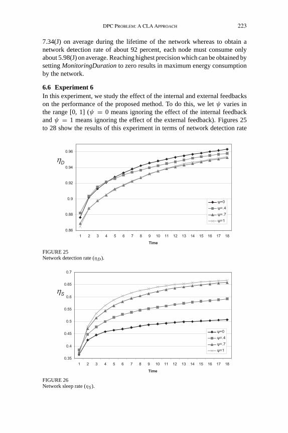
6.6 Experiment 6In this experiment, we study the effect of the internal and external feedbackson the performance of the proposed method. To do this, we letψ varies inthe range [0, 1] (ψ = 0 means ignoring the effect of the internal feedbackandψ = 1 means ignoring the effect of the external feedback). Figures 25to 28 show the results of this experiment in terms of network detection rate

0.86

0.88

0.9

0.92

0.94

0.96

1 2 3 4 5 6 7 8 9 10 11 12 13 14 15 16 17 18

Time

=0

=.4

=.7

=1

D


0.35

0.4

0.45

0.5

0.55

0.6

0.65

0.7

1 2 3 4 5 6 7 8 9 10 11 12 13 14 15 16 17 18

Time

=0

=.4

=.7

=1

S


“aswin150” — 2010/3/12 — 9:37 — page 224 — #32


0.2

0.25

0.3

0.35

0.4

0.45

1 2 3 4 5 6 7 8 9 10 11 12 13 14 15 16 17 18

Time

=0

=.4

=.7

=1R


2

2.5

3

3.5

4

4.5

5

5.5

6

6.5

7

1 2 3 4 5 6 7 8 9 10 11 12 13 14 15 16 17 18

Time

Co

nsu

med

En

erg

y (

J)

=0

=.4

=.7

=1


(ηD), network sleep rate (ηS), network redundant active rate (ηR) and meanenergy consumption of the nodes. From these figures we can conclude that1. decreasing the effect of the internal feedback in equation (9) by decreas-ing parameterψ results in more network detection rate at the expense ofmore energy consumption, more redundant active times and less sleep times.2. Increasing the effect of the internal feedback in equation (9) by increasingparameterψresults in more energy saving in the network at the expense oflower network detection rate.

“aswin150” — 2010/3/12 — 9:37 — page 225 — #33


6.7 Experiment 7Experiment 6 has shown that the internal and external feedbacks have differenteffects on the performance of the proposed algorithm in terms of networkdetection rate (ηD), network sleep rate (ηS), network redundant active rate(ηR) and mean energy consumption of the nodes. The results reported inexperiment 6 are holding only if the number of sensors in the network remainsunchanged. This is because of the fact that the accuracy of external feedbackof sensor nodesk starts degrading as the number of its neighboring sensorsstarts to decrease due to malfunctioning or energy depletion. Lesser numberof neighboring sensors for a sensor means that the probability of accuracy ofinformation obtained about the surrounding environment decreases. When theaccuracy of the external feedback reduces, a node has to depends on its owninformation about the movement pattern of target points obtained using itssensing unit. Therefore, if a node wants its detection rate not to fall too much,then it has to let its sensing unit be in active state more often, which meansmore energy consumption.

One way to reduce the effect of the external feedback as the number ofnodes reduces is to use a time varyingψsuch as the one given in equation(16). In equation 16ψ for each sensor node is defined to be a function of thenumber of neighbors of the node.

ψnk =N(sk)−Nn(sk)

N(sk); N(sk) �= 0

1; N(sk) = 0(16)

In equation (16),Nn(sk) is the number of neighbors ofsk in thenth activationof ck of the ICLA.

In this experiment, we study the performance of the proposed algorithmwhenψvaries according to the equation (16). We compare the results obtainedfor the proposed algorithm for a fixed value ofψ (ψ = .4) and a time vary-ingψ . Figures 29 to 32 show the results of this experiment in terms of networkdetection rate (ηD), network sleep rate (ηS), network redundant active rate (ηR)and mean energy consumption of the nodes. These figures show that using atime varyingψenhances the network detection rate at the expense of moreenergy consumption, more redundant active times and less sleep times.

6.8 Experiment 8This experiment is conducted to study the effect of the number of reporternodes on the performance of the proposed method. As we stated before, forplacing the reporter nodes, the simulation environment is divided into a numberof square cells and one reporter node is placed on each boundary point ofcells. The experiment is conducted for different sizes of the square cells:14(m)×14(m), 10(m)×10(m), 7(m)×7(m) and 5(m)×5(m). The numberof reporter nodes (M) for these cases will be 49, 100, 196 and 500 respectively.

“aswin150” — 2010/3/12 — 9:37 — page 226 — #34


0.845

0.855

0.865

0.875

0.885

0.895

0.905

0.915

0.925

1 2 3 4 5 6 7 8 9 10 11 12 13 14 15 16 17 18 19 20 21 22 23 24

Time

Static

Time Varying

D


0.4

0.45

0.5

0.55

0.6

0.65

1 2 3 4 5 6 7 8 9 10 11 12 13 14 15 16 17 18 19 20 21 22 23 24

Time

Static

Time Varying

S


0.29

0.31

0.33

0.35

0.37

0.39

0.41

0.43

1 2 3 4 5 6 7 8 9 10 11 12 13 14 15 16 17 18 19 20 21 22 23 24

Time

Static

Time Varying

R


“aswin150” — 2010/3/12 — 9:37 — page 227 — #35


0

0.5

1

1.5

2

2.5

1 2 3 4 5 6 7 8 9 10 11 12 13 14 15 16 17 18 19 20 21 22 23 24

Time

Co

nsu

med

En

erg

y (

J)

Static

Time Varying


0.8

0.82

0.84

0.86

0.88

0.9

0.92

1 3 5 7 9 11 13 15 17 19 21 23 25 27 29

Time

Reporter Nodes=500

Reporter Nodes=196

Reporter Nodes=100

ReporterNodes=49

D


Figures 33 through 36 show the results of this experiment in terms of networkdetection rate (ηD), network sleep rate (ηS), network redundant active rate(ηR) and mean energy consumption of the nodes. These figures show that asthe number of reporter nodes (M) increases from 49 to 196,ηDandηRdecreaseandηSand mean energy consumption of the nodes increase. Further increasein M beyond 196, has no significant effect onηD, ηR, ηS and mean energyconsumption of the nodes. The reason for this is that by increasing the numberof reporter nodes from 49 to 196, the number of neighbors of each sensor nodedecreases which according to the results of experiment 7, reduces the accuracyof the external feedbacks of sensor nodes. WhenM = 196, no sensor nodein the network has a neighbor and for this reason increasingM beyond 195

“aswin150” — 2010/3/12 — 9:37 — page 228 — #36


0.37

0.42

0.47

0.52

0.57

0.62

0.67

1 3 5 7 9 11 13 15 17 19 21 23 25 27 29

Time

Reporter Nodes=500

Reporter Nodes=196

Reporter Nodes=100

ReporterNodes=49

S


0.25

0.27

0.29

0.31

0.33

0.35

0.37

0.39

0.41

0.43

0.45

1 3 5 7 9 11 13 15 17 19 21 23 25 27 29

Time

Reporter Nodes=500

Reporter Nodes=196

Reporter Nodes=100

ReporterNodes=49

R


0

1

2

3

4

5

6

7

1 3 5 7 9 11 13 15 17 19 21 23 25 27 29

Time

Co

nsu

me

d E

ne

rgy

(J

)

Reporter Nodes=500

Reporter Nodes=196

Reporter Nodes=100

ReporterNodes=49


“aswin150” — 2010/3/12 — 9:37 — page 229 — #37


has no effect on the number of neighbors of sensor nodes. This implies thatincreasingM beyond 196 will have no significant effect onηD, ηR, ηS andmean energy consumption of the nodes.

7 CONCLUSION

In this paper, an algorithm based on irregular cellular learning automata(ICLA) for the problem of detecting and monitoring a number of movingtarget points in an area by sensor networks was proposed. The sensor networkwas mapped into an ICLA. The learning automaton residing in each cell of theICLA in cooperation with the learning automata residing in the neighboringcells dynamically predicts the existence of any target points in the vicinityof its corresponding node in the network in near future. This prediction isthen used to schedule the active times of that node. The experimental resultsshowed that there exists a parameter in the proposed method which can betuned so that one can save more energy in the network at the expense of lesserprecision or has more precision at the expense of lower network lifetime. Infact determination of this parameter for an application is very crucial and is amatter of cost versus precision. Furthermore, the experimental results showedthat the proposed algorithm is robust against changes in the parameters of thetarget points’ movement patterns such as the velocity of moving targets andthe frequency of occurrences of events.

REFERENCES

[1] M. Ilyas and I. Mahgoub.Handbook of Sensor Networks: Compact Wireless and WiredSensing Systems. CRC Press, London, Washington, D.C., 2005.

[2] H. Chen, H. Wu and N.-F. Tzeng. Grid-based Approach for Working Node Selection inWireless Sensor Networks.Proc. of IEEE Intl. Conf. on Communications 2004 (ICC 2004),2004.

[3] Y. Zou and K. Chakrabarty. A Distributed Coverage- and Connectivity-Centric Techniquefor Selecting Active Nodes in Wireless Sensor Networks.IEEE Transactions on Computers54(8), 978–991, August 2005.

[4] F. Pedraza,A. García andA. L. Medaglia. Efficient CoverageAlgorithms forWireless SensorNetworks.in Proc. of the 2006 Systems and Information Engineering Design Symposium,2006.

[5] Zh. Dingxing, X. Ming, Ch. Yingwen and W. Shulin. Probabilistic Coverage Configurationfor Wireless Sensor Networks.2nd Intl. Conf. on Wireless Communications, Networkingand Mobile Computing (WiCOM 2006), Wuhan, September 2006.

[6] R. Gupta and S. R. Das. Tracking Moving Targets in a Smart Sensor Network.Proc. IEEEVTC 5, 3035–3039, October 2003.

[7] Ch. Gui and P. Mohapatra. Power Conservation and Quality of Surveillance in TargetTracking Sensor Networks.Proc. of the 10th Annual Intl. Conf. on Mobile Computing andNetworking (MOBICOM 2004), Philadelphia, PA, USA, September–October, 2004.

[8] G. He and J. C. Hou. Tracking Targets with Quality in Wireless Sensor Networks.13th IEEEIntl. Conf. on Network Protocols (ICNP 2005), Boston, MA, USA, November 2005.

“aswin150” — 2010/3/12 — 9:37 — page 230 — #38


[9] M. K.Watfa and S. Commuri.AReduced CoverApproach to Energy EfficientTracking usingWireless Sensor Networks.World Congress in Computer Sceince, Computer Engineeringand Applied Computing, Las Vegas, Nevada, USA, June 2006.

[10] J. Jeong, S. Sharafkandi and D. H. C. Du. Energy-aware scheduling with quality ofsurveillance guarantee in wireless sensor networks.Intl. Conf. on Mobile Computing andNetworking, Los Angeles, CA, USA, 2006.

[11] J. Jeong, T. Hwang, T. He and D. Du. MCTA: Target Tracking Algorithm based on MinimalContour in Wireless Sensor Networks.In IEEE Infocom2007 Minisymposia, August 2007.

[12] V. Raghunathan, C. Schurgers, S. Park and M. B. Srivastava. Energy-Aware Wireless sensornetworks.IEEE Singal Processing Magazine, 2002–03.

[13] K. Chakrabarty, S. S. Iyengar, H. Qi and E. Cho. Grid coverage for surveillance and targetLocation in distributed sensor networks.IEEE Transactions on Computers 51, 1448–1453,2002.

[14] G. Bontempi and Y. Le Borgne. An adaptive modular approach to the mining of sensornetwork data.Workshop on Data Mining in Sensor Networks, SIAM SDM, Newport Beach,CA, USA, April 2005.

[15] C. Liu, K. Wu and J. Pei. ADynamic Clustering and SchedulingApproach to Energy Savingin Data Collection from Wireless Sensor Networks.In Proceedings of the Second AnnualIEEE Communications Society Conference on Sensor and Ad Hoc Communications andNetworks (SECON’05), Santa Clara, California, USA, September, 2005.

[16] O.Younis and S. Fahmy. An Experimental Study of Routing and DataAggregation in SensorNetworks.In Proceedings of the International Workshop on Localized Communication andTopology Protocols for Ad hoc Networks (LOCAN), held in conjunction with The 2nd IEEEInternational Conference on Mobile Ad Hoc and Sensor Systems (MASS-2005), November2005.

[17] R. Virrankoski and A. Savvides. TASC: Topology Adaptive Spatial Clustering for SensorNetworks.Second IEEE Intl. Conf. on Mobile Ad Hoc and Sensor Systems, Washington,DC, November, 2005.

[18] S. Soro and W. Heinzelman. Prolonging the Lifetime of Wireless Sensor Networks viaUnequal Clustering.Proceedings of the 5th International Workshop on Algorithms forWireless, Mobile, Ad Hoc and Sensor Networks (IEEE WMAN ’05), April 2005.

[19] W. Heinzelman, A. Chandrakasan and H. Balakrishnan. Energy-efficient communicationprotocol for wireless microsensor networks.Proc. of 33rd Hawaii Intl. Conf. on SystemScience (HICSS ’00), January 2000.

[20] O. Younis and S. Fahmy. Distributed Clustering in Ad-hoc Sensor Networks: A Hybrid,Energy-Efficient Approach. InProc. of IEEE INFOCOM 1, 629–640, March 2004.

[21] S. P. Chaudhuri and D. B. Johnson. An Adaptive Scheduling Protocol for Multi-scale Sen-sor Network Architecture.IEEE Intl. Conf. on Distributed Computing in Sensor Systems(DCOSS), Santa Fe, New Mexico, June 2007.

[22] A. M. Chou and V. Li. Slot Allocation Strategies for TDMA Protocols in Multihop PacketRadio Networks.In Proceedings of INFOCOM, pp. 710–716, 1992.

[23] I. Chlamtac and A. Farago. Making Transmission Schedules Immune to Topology Changesin Multi-hop Packet Radio Networks.IEEE/ACM Transactions on Networks 2, 23–29, 1994.

[24] V. Rajendran, K. Obraczka and J. J. Garcia-Luna-Aceves. Energy-efficient Collision-FreeMedium Access Control for Wireless Sensor Networks.In Proceedings of the First Intl.Conf. on Embedded Networked Sensor Systems (Sensys’03), New York, pp. 181–192,2003.

[25] L. Bao and J. J. Garcia-Luna-Aceves. A New Approach to Channel Access Scheduling forAd hoc Networks.In Proceedings of the 7th Annual International Conference on MobileComputing and Networking (MobiCom’01), New York, pp. 210–221, 2001.

[26] M. Sichitiu. Cross-Layer Scheduling for Power Efficiency in Wireless Sensor Networks. InProc. of IEEE INFOCOM, volume 1, March 2004.

“aswin150” — 2010/3/12 — 9:37 — page 231 — #39


[27] Y. Nam, T. Kwon, H. Lee, H. Jung and Y. Choi. Guaranteeing the network lifetime inwireless sensor networks: A MAC Layer Approach.Elsevier Computer Communications30, 2532–2545, June 2007.

[28] Sh. Liu, K. W. Fan and P. Sinha. Dynamic Sleep Scheduling using Online Experimentationfor Wireless Sensor Networks.In Proceeding of SenMetrics, San Diego, July 2005.

[29] Y. Xu, J. S. Heidemann and D. Estrin. Geography-informed energy conservation for ad hocrouting.In Proceedings of Mobile Computing and Networking, pp. 70–84, 2001.

[30] J. Salzmann, S. Kubisch, F. Reichenbach and D. Timmermann. Energy and CoverageAware RoutingAlgorithm in Self Organized Sensor Networks.In Proceedings of NetworkedSensing Systems (INSS’07), June 2007.

[31] C. Schurgers, V. Tsiatsis and M. Srivastava. STEM: Topology management for energyefficient sensor networks.In Proceedings of the IEEE Aerospace Conference, March 2002.

[32] R. Akl and U. Sawant. Grid-based Coordinated Routing in Wireless Sensor Networks.InProceedings of 4th IEEE Conf. on Computer Communications and Networking, January2007.

[33] G. Wang, G. Cao, T. La Porta and W. Zhang. Sensor Relocation in Mobile Sensor Networks.In Proceedings of IEEE INFOCOM, March 2005.

[34] J. N. Al-Karaki, R. Ul-Mustafa and A. E. Kamal. Data aggregation in wireless sensornetworks – exact and approximate algorithms.In Proceedings of IEEE Workshop on HighPerformance Switching and Routing, pp. 241–245, April 2004.

[35] F. Araújo and L. Rodrigues. On the Monitoring Period for Fault-Tolerant Sensor Networks.In Proceedings of Latin-American Symposium on Dependable Computing, pp. 174–190,2005.

[36] Z. Jiang, J. Wu, A. Agah and B. Lu. Topology Control for Secured Coverage in WirelessSensor Networks.In Proceedings of 3rd IEEE Intl. Workshop on Wireless and SensorNetworks Security (WSNS’07), October 2007.

[37] R. P. Liu, G. Rogers, S. Zhou and J. Zic. Topology control with Hexagonal Tessellation.Intl. Journal of Sensor Networks 2(1/2), 91–98, 2007.

[38] R. P. Liu, G. Rogers and S. Zhou. Honeycomb Architecture for Energy Conservation inWireless Sensor Networks. InProceedings of IEEE Globecom, San Francisco, November2006.

[39] Y. Wu, S. Fahmy and N. B. Shroff. Optimal QoS-Aware Sleep/Wake Scheduling forTime-Synchronized Sensor Networks.Invited Sessions on Optimization of Communica-tion Networks 40th Annual Conf. on Information Sciences and Systems (CISS), Princeton,NJ, 2006.

[40] M. Bagheri and M. Hefeeda. Randomized k-Coverage Algorithms For Dense Sensor Net-works.in Proc. of IEEE INFOCOM 2007 Minisymposium, Anchorage, AK, pp. 2376–2380,May 2007.

[41] M. Bagheri, M. Hefeeda and H. Ahmadi. A Near Optimal K-Coverage Algorithm for Large-scale Sensor Networks. Technical ReportTR 2006-10, School of Computing Science, SimonFraser University, Burnaby, BC, Canada, May 2006.

[42] B. Wang, K.C. Chua, V. Srinivasan and W. Wang. Scheduling Sensor Activity for PointInformation Coverage in Wireless Sensor Networks.In Proc. of WiOpt, 2006.

[43] B. Wang, K.C. Chua, V. Srinivasan and W. Wang. Sensor Density for Complete InformationCoverage in Wireless Sensor Networks.In Proc. of EWSN 2006, Zurich, Switzerland,February 2006.

[44] B. Liang, J. Frolik and X. S. Wang. A Predictive QoS Control Strategy for Wireless SensorNetworks.The 1st Workshop on Resource Provisioning and Management in Sensor Net-works (PRMSN 05) in Conjunction with the 2nd IEEE MASS, Washington DC, November2005.

[45] J. Frolik. QoS Control for Random Access Wireless Sensor Networks.Wireless Communi-cations and Networking Conf. (WCNC04), Atlanta, March 2004.

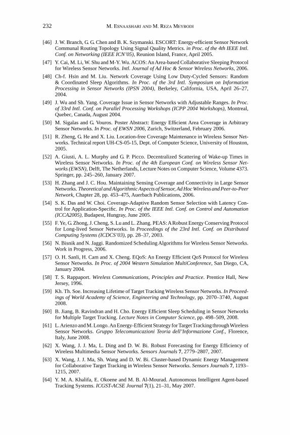
“aswin150” — 2010/3/12 — 9:37 — page 232 — #40


[46] J. W. Branch, G. G. Chen and B. K. Szymanski. ESCORT: Energy-efficient Sensor NetworkCommunal Routing Topology Using Signal Quality Metrics.in Proc. of the 4th IEEE Intl.Conf. on Networking (IEEE ICN’05), Reunion Island, France, April 2005.

[47] Y. Cai, M. Li, W. Shu and M-Y. Wu. ACOS:AnArea-based Collaborative Sleeping Protocolfor Wireless Sensor Networks.Intl. Journal of Ad Hoc & Sensor Wireless Networks, 2006.

[48] Ch-f. Hsin and M. Liu. Network Coverage Using Low Duty-Cycled Sensors: Random& Coordinated Sleep Algorithms.In Proc. of the 3rd Intl. Symposium on InformationProcessing in Sensor Networks (IPSN 2004), Berkeley, California, USA, April 26–27,2004.

[49] J. Wu and Sh. Yang. Coverage Issue in Sensor Networks with Adjustable Ranges.In Proc.of 33rd Intl. Conf. on Parallel Processing Workshops (ICPP 2004 Workshops), Montreal,Quebec, Canada, August 2004.

[50] M. Sigalas and G. Vouros. Poster Abstract: Energy Efficient Area Coverage in ArbitrarySensor Networks.In Proc. of EWSN 2006, Zurich, Switzerland, February 2006.

[51] R. Zheng, G. He and X. Liu. Location-free Coverage Maintenance in Wireless Sensor Net-works. Technical report UH-CS-05-15, Dept. of Computer Science, University of Houston,2005.

[52] A. Giusti, A. L. Murphy and G. P. Picco. Decentralized Scattering of Wake-up Times inWireless Sensor Networks.In Proc. of the 4th European Conf. on Wireless Sensor Net-works (EWSN), Delft, The Netherlands, Lecture Notes on Computer Science, Volume 4373.Springer, pp. 245–260, January 2007.

[53] H. Zhang and J. C. Hou. Maintaining Sensing Coverage and Connectivity in Large SensorNetworks.Theoretical and Algorithmic Aspects of Sensor, Ad Hoc Wireless and Peer-to-PeerNetwork, Chapter 28, pp. 453–475, Auerbach Publications, 2006.

[54] S. K. Das and W. Choi. Coverage-Adaptive Random Sensor Selection with Latency Con-trol for Application-Specific.In Proc. of the IEEE Intl. Conf. on Control and Automation(ICCA2005), Budapest, Hungray, June 2005.

[55] F.Ye, G. Zhong, J. Cheng, S. Lu and L. Zhang. PEAS:ARobust Energy Conserving Protocolfor Long-lived Sensor Networks. InProceedings of the 23rd Intl. Conf. on DistributedComputing Systems (ICDCS’03), pp. 28–37, 2003.

[56] N. Bisnik and N. Jaggi. Randomized Scheduling Algorithms for Wireless Sensor Networks.Work in Progress, 2006.

[57] O. H. Sanli, H. Cam and X. Cheng. EQoS: An Energy Efficient QoS Protocol for WirelessSensor Networks.In Proc. of 2004 Western Simulation MultiConference, San Diego, CA,January 2004.

[58] T. S. Rappaport.Wireless Communications, Principles and Practice. Prentice Hall, NewJersey, 1996.

[59] Kh. Th. Soe. Increasing Lifetime of Target Tracking Wireless Sensor Networks.In Proceed-ings of World Academy of Science, Engineering and Technology, pp. 2070–3740, August2008.

[60] B. Jiang, B. Ravindran and H. Cho. Energy Efficient Sleep Scheduling in Sensor Networksfor Multiple Target Tracking.Lecture Notes in Computer Science, pp. 498–509, 2008.

[61] L.Arienzo and M. Longo.An Energy-Efficient Strategy forTargetTracking throughWirelessSensor Networks.Gruppo Telecomunicazioni Teoria dell’Informazione Conf., Florence,Italy, June 2008.

[62] X. Wang, J. J. Ma, L. Ding and D. W. Bi. Robust Forecasting for Energy Efficiency ofWireless Multimedia Sensor Networks.Sensors Journals 7, 2779–2807, 2007.

[63] X. Wang, J. J. Ma, Sh. Wang and D. W. Bi. Cluster-based Dynamic Energy Managementfor Collaborative Target Tracking in Wireless Sensor Networks.Sensors Journals 7, 1193–1215, 2007.

[64] Y. M. A. Khalifa, E. Okoene and M. B. Al-Mourad. Autonomous Intelligent Agent-basedTracking Systems.ICGST-ACSE Journal 7(1), 21–31, May 2007.

“aswin150” — 2010/3/12 — 9:37 — page 233 — #41


[65] M. K. Watfa. An Energy Efficient Approach to Dynamic Coverage in Wireless SensorNetworks.Journal of Networks 1(4), 10–20, August 2006.

[66] T. He, P. Vicaire, T. Yan, L. Luo, L. Gu and G. Zhou. Achieving Real-Time Target TrackingUsing Wireless Sensor Networks.In Proc. of the 12th IEEE Real-Time and EmbeddedTechnology and Applications Symposium (RTAS’06), April 2006.

[67] H. Yang and B. Sidkar. Lightweight Target Tracking Protocol Using Ad hoc SensorNetworks.In Proceedings of IEEE VTC, Stockholm, Sweden, May 2005.

[68] S. Bhattacharya, G. Xing, Ch. Lu, G.C. Roman, O. Chipara and B. Harris. Dynamic Wake-up and Topology Maintenance Protocol with Spatiotemporal Guarantees.In Proceedingsof 4th International Symposium on Information Processing in Sensor Networks, pp. 28–34,2005.

[69] W. Zhang and G. Cao. Optimizing Tree Reconfiguration for Mobile Target Tracking inSensor Networks.In Proceedings of Twenty-third Annual Joint Conf. of INFOCOM, vol. 4,pp. 2434–2445, 2004.

[70] http://www.nytimes.com/2008/07/12/business/12newpark.html

[71] A. Sobeih, W. P. Chen, J. C. Hou, L. C. Kung, N. Li, H. Lim, H.Y. Tyan and H. Zhang. J-Sim:A Simulation and Emulation Environment for Wireless Sensor Networks.IEEE WirelessCommunications 13(4), 104–119, August 2006.

[72] L. Wang and Y. Ziao. A Survey of Energy-Efficient Scheduling Mechanisms in SensorNetworks.Mobile Networks and Applications 11(5), 723–740, 2006.

[73] C. Bettstetter, H. Hartenstein and X. Pérez-Costa. Stochastic Properties of the RandomWaypoint Mobility Model. ACM/Kluwer Wireless Networks: Special Issue on Modelingand Analysis of Mobile Networks 10(5), 555–567, September 2004.

[74] E. Fredkin. Digital machine:An informational process based on reversible cellular automata.Physica D45, 245–270, 1990.

[75] M. A. L. Thathachar and P. S. Sastry. Varieties of Learning Automata: An Overview.IEEETransaction on Systems, Man, and Cybernetics-Part B: Cybernetics 32(6), 711–722, 2002.

[76] K. S. Narendra and M.A. L. Thathachar.Learning Automata: An Introduction. Prentice-HallInc, 1989.

[77] M. R. Kharazmi and M. R. Meybodi. Image Segmentation Using Cellular LearningAutomata.In Proc. of 10th Iranian Conf. on Electrical Engineering, ICEE-96, Tabriz,Iran, May 2001.

[78] M. R. Kharazmi and M. R. Meybodi. Image Restoration Using Cellular LearningAutomata.In Proc. of 2nd Iranian Conf. on Machine Vision, Image Processing and Applications,Tehran, Iran, pp. 261–270, 2003.

[79] M. R. Meybodi, H. Beygi and M. Taherkhani. Cellular Learning Automata and its Applica-tions.Journal of Science Tech., Sharif (Sharif University of Technology, Tehran, Iran), pp.54–77, 2004.

[80] M. R. Meybodi and M. R. Khojaste. Application of Cellular LearningAutomata in Modelingof Commerce Networks.In Proc. of 6th Annual Intl. Computer Society of Iran ComputerConf., CSICC-2001, Isfehan, Iran, pp. 284–295, February 2001.

[81] M. R. Meybodi and M. Taherkhani. Application of Cellular LearningAutomata in Modelingof Rumor Diffusion.In Proc. of 9th Conf. on Electrical Engineering, Power and WaterInstitute of Technology, Tehran, Iran, pp. 102–110, May 2001.

[82] H. Beigy and M. R. Meybodi. ASelf-Organizing ChannelAssignmentAlgorithm: ACellularLearning Automata Approach.Springer-Verlag Lecture Notes in Computer Science, vol.2690, pp. 119–126, 2003.

[83] H. Beigy and M. R. Meybodi. Call Admission in Cellular Networks: A Learning AutomataApproach.Springer-Verlag Lecture Notes in Computer Science, vol. 2510, pp. 450–457,2002.

[84] H. Beigy and M. R. Meybodi. A Mathematical Framework for Cellular Learning Automata.Advances in Complex Systems7(3 & 4), 295–319, September & December 2004.

“aswin150” — 2010/3/12 — 9:37 — page 234 — #42


[85] H. Beigy and M. R. Meybodi. Open Synchronous Cellular Learning Automata.Advancesin Complex Systems 10(4), 1–30, December 2007.

[86] H. Beigy and M. R. Meybodi. Asynchronous Cellular Learning Automata.Automatica44(5), 1350–1357, May 2008.

[87] M. Esnaashari and M. R. Meybodi. A Cellular Learning Automata based ClusteringAlgorithm for Wireless Sensor Networks.Sensor Letters 6(5), 723–735, December 2008.

[88] S. Meguerdichian, F. Koushanfar, M. Potkonjak and M. B. Srivastava. Coverage Problemsin Wireless Ad-Hoc Sensor Networks.In Proc. of the IEEE INFOCOM ’01, the Conferenceon Computer Communications, vol. 3, pp. 1380–1387, April 2001.

[89] F. Ye, S. Lu and L. Zhang. A Randomized Energy-Conservation Protocol for ResilientSensor Networks.Wireless Networks 12(5), 637–652, October 2006.

Documents

Dynamic Point Coverage Problem in Wireless Sensor ...ceit.aut.ac.ir/~meybodi/paper/Esnaashari-2010-ad hoc and...One way to prolong the lifetime of a wireless sensor network is to schedule