Embed Size (px)
Citation preview
1
Learning Automatabased Algorithms for Solving Stochastic Minimum Spanning Tree Problem
Javad Akbari Torkestani Department of Computer Engineering, Islamic Azad University, Arak Branch, Arak, Iran
j‐akbari@iau‐arak.ac.ir
Mohammad Reza Meybodi Department of Computer Engineering and IT, Amirkabir University of Technology, Tehran, Iran
Institute for Studies in Theoretical Physics and Mathematics (IPM), School of Computer Science, Tehran, Iran [email protected]
Abstract Due to the hardness of solving the minimum spanning tree (MST) problem in stochastic environments, the stochastic MST (SMST) problem has not received the attention it merits, specifically when the probability distribution function (PDF) of the edge weight is not a priori known. In this paper, we first propose a learning automata‐based sampling algorithm (Algorithm 1) to solve the MST problem in stochastic graphs where the PDF of the edge weight is assumed to be unknown. At each stage of the proposed algorithm, a set of learning automata is randomly activated and determines the graph edges that must be sampled in that stage. As the proposed algorithm proceeds, the sampling process focuses on the spanning tree with the minimum expected weight. Therefore, the proposed sampling method is capable of decreasing the rate of unnecessary samplings and shortening the time required for finding the SMST. The convergence of this algorithm is theoretically proved and it is shown that by a proper choice of the learning rate the spanning tree with the minimum expected weight can be found with a probability close enough to unity. Numerical results show that Algorithm 1 outperforms the standard sampling method. Selecting a proper learning rate is the most challenging issue in learning automata theory by which a good trade off can be achieved between the cost and efficiency of algorithm. To improve the efficiency (i.e., the convergence speed and convergence rate) of Algorithm 1, we also propose four methods to adjust the learning rate in Algorithm 1 and the resultant algorithms are called as Algorithm 2 through Algorithm 5. In these algorithms, the probabilistic distribution parameters of the edge weight are taken into consideration for adjusting the learning rate. Simulation experiments show the superiority of Algorithm 5 over the others. To show the efficiency of Algorithm 5, its results are compared with those of the multiple edge sensitivity method (MESM). The obtained results show that Algorithm 5 performs better than MESM both in terms of the running time and sampling rate.
Keyword: Learning automata, Minimum spanning tree, Stochastic graph
1. Introduction A minimum spanning tree (MST) of an edge‐weighted network is a spanning tree having the minimum sum
of edge weights among all spanning trees. The weight associated with the graph edge represents its cost, traversal time, or length depending on the context. Minimum spanning tree has many applications in different areas such as data storage [31, 32], statistical cluster analysis [33, 34], picture processing [35], and especially in communication networks [36, 37]. In network routing protocols, the minimum cost spanning tree is one of the most effective methods to multicast or broadcast the massages from a source node to a set of destinations. In most scenarios, the edge weight is assumed to be fixed, but this does not hold always true and they vary with time in real applications. For example, the links in a communication network may be affected by collisions, congestions and interferences. Therefore, the MST problem is generalized toward a stochastic minimum spanning tree (SMST) problem in which the edge weight is a random variable rather than a constant value. There have been many studies of the minimum spanning tree problem dealing with the deterministic graphs and several well‐known sequential algorithms such as Boruvka [1], Kruskal [2] and Prim [3], in which the MST problem can be solved in polynomial time, have been presented. Furthermore, several efficient
2
distributed [20‐24] and approximation [25‐27] algorithms have been also proposed to solve the MST problem in deterministic graphs. However, when the edge weight is allowed to be random (vary with time), this problem becomes considerably hard to solve. This becomes more difficult if the probability distribution function (PDF) of the edge weight is not a priori known. Unlike the deterministic graphs, due to hardness the MST problem has not received much attention in stochastic graphs.
Ishii et al. [4] proposed a method for solving the stochastic spanning tree problem in which the mentioned problem is transformed into its proxy deterministic equivalent problem and then a polynomial time algorithm presented to solve the latter problem. In this method, the probability distribution of the edges' weights is assumed to be known. Ishii and Nishida [5] considered a stochastic version of the bottleneck spanning tree problem on the edges whose weights are random variables. They showed that, under reasonable restrictions, the problem can be reduced to a minimum bottleneck spanning tree problem in a deterministic case. Mohd [6] proposed a method for stochastic spanning tree problem called interval elimination and introduced several modifications to the algorithm of Ishii et al. [4] and showed that the modified algorithm is able to obtain the better results in less time. Ishii and Matsutomi [7] presented a polynomial time algorithm to solve the problem stated in [4] when the probability distribution of the edges weight is unknown. They applied a statistical approach to a stochastic spanning tree problem and considered a minimax model of the stochastic spanning tree problems with a confidence region of unknown distribution parameters. Alexopoulos and Jacobson [8] proposed some methods to determine the probability distribution of the weight of the MST in stochastic graphs in which the edges have independent discrete random weights, and the probability that a given edge belongs to a minimum spanning tree. Dhamdhere et al. [9] and Swamy and Shmoys [10] formulated the stochastic MST problem as a stochastic optimization problem and proposed some approximation approaches to solve two and multistage stochastic optimization problems.
In [41], Hutson and Shier studied several approaches to find (or to optimize) the minimum spanning tree when the edges undergo the weight changes. Repeated Prim method, cut‐set method, cycle tracing method, and multiple edge sensitivity method are the proposed approaches to find the MST of the stochastic graph in which the edge weight can assume a finite number of distinct values as a random variable. To approximate the expected weight of the optimal spanning tree, Hutson and Shier used the algebraic structure to describe the relationship between the different edge‐weight realizations of the stochastic graph. They compared different approaches and showed that the multiple edge sensitivity method, which is here referred to as MESM, outperforms the others in terms of the time complexity and the size of the constructed state space. Katagiri et al. [38] introduced a fuzzy‐based approach to model the minimum spanning tree problem in case of fuzzy random weights. They examined the case where the edge weights are fuzzy random variables. Fangguo and Huan [39] considered the problem of minimum spanning tree in uncertain networks in which the edge weights are random variables. They initially define the concept of the expected minimum spanning tree and mathematically model (formulate) the problem accordingly. Then, based on the resulting model they propose a hybrid intelligent algorithm which is a combination of the genetic algorithm and a stochastic simulation technique to solve the SMST problem. In [44], a new classification is presented for MST algorithms. This paper generally classifies the existing approaches into deterministic and stochastic MST algorithms. Deterministic algorithms are further subdivided into constrained and unconstrained classes. In this paper, the authors propose a heuristic method to solve the stochastic version of the minimum spanning tree problem. In [39], the Prüfer encoding scheme which is able to represent all possible trees is used to code the corresponding spanning trees in the genetic representation. Almeida et al. [40] studied the minimum spanning tree problem with fuzzy parameters and proposed an exact algorithm to solve this problem.
The main drawback of the above mentioned SMST algorithms is that they are feasible only when the probability distribution function of the edge weight is assumed to be a priori known, whereas this assumption can not hold true in realistic applications. In this paper, we first propose a learning automata‐based approximation algorithm called Algorithm 1 to solve the minimum spanning tree problem in a stochastic graph, where the probability distribution function of the edge weight is unknown. As Algorithm 1 proceeds, the process of sampling from the graph is concentrated on the edges of the spanning tree with the minimum expected weight. This is theoretically proved for Algorithm 1 that by the proper choice of the learning rate the spanning tree with the minimum expected weight will be found with a probability close enough to unity. To show the performance of Algorithm 1, the number of samples that is required to be taken from the stochastic graph by this algorithm is compared with that of the standard sampling method when the approximated value of the edge weight converges to its mean value with a certain probability. The obtained results show that the average number of samples taken by Algorithm 1 is much less than that of the standard sampling method. In
3
Algorithm 1, a learning automaton is assigned to each graph node and the incident edges of node are defined as its action‐set. This algorithm is composed of a number of stages and at each stage a spanning tree of the graph is constructed by the random selection of the graph edges by the activated automata. At each stage, if the expected weight of the constructed spanning tree is larger than the average weight of all spanning trees constructed so far, the constructed spanning tree is penalized and it is rewarded otherwise. The performance of a learning automata‐based algorithm is directly affected by the learning rate. Choosing the same learning rate for all learning automata to update their action probability vectors may prolong the convergence for some learning automata and accelerate the convergence to a non‐optimal solution for some others. To avoid this, we also propose four methods for adjusting the learning rate and apply them to Algorithm 1. Algorithm 1 in which the learning rate is computed by these four statistical methods are named as Algorithm 2 through Algorithm 5. Computer simulation shows that Algorithm 5 outperforms the others in terms of sampling rate (the number of samples) and convergence rate. To investigate the efficiency of the best proposed algorithm (Algorithm 5), we compare Algorithm 5 with MESM proposed by Hutson and Shier [41]. The obtained results show that Algorithm 5 is superior to MESM in terms of running time and sampling rate.
The rest of the paper is organized as follows. The stochastic graph and learning automata theory are briefly reviewed in section 2. In section 3, our learning automata‐based algorithms are presented. Section 4 presents the convergence proof of the first proposed algorithm (Algorithm 1) and studies the relationship between the learning rate and convergence rate of Algorithm 1. Section 5 evaluates the performance of the proposed algorithms through simulation experiments, and Section 6 concludes the paper.
2. Stochastic Graph, Learning Automata Theory To provide the sufficient background for understanding the basic concepts of the Stochastic minimum
spanning tree algorithms which are presented in this paper, the stochastic graphs and learning automata theory are briefly described in this section.
2.1. Stochastic Graph An undirected stochastic graph G can be defined by a triple ),Ε,(= WVG , where },...,,{ 21 nvvvV = is the
vertex set, VVE ×⊂ is the edge set, and matrix nnW × denotes the probability distribution function of the random weight associated with the graph edges, where n is the number of nodes. For each edge ),( jie the
associated weight is assumed to be a positive random variable with probability density function jiw , , which is assumed to be unknown in this paper. An undirected stochastic sub‐graph ),Ε′,′(=′ WVG is also called a stochastic spanning tree of G if ′G is a connected sub‐graph, ′G has the same edge set asG , and EE ⊆′ , satisfying 1n-|E| =′ , where |E| ′ denotes the cardinality of set E′ . Let },,,{ 321 Kτττ=T be the set of all possible
stochastic spanning trees of graphG and iWτ denotes the expected weight of spanning tree iτ . SMST is defined as the stochastic spanning tree with the minimum expected weight. In other words, a given stochastic minimum spanning tree T∈*τ is the SMST if and only if }{min*
iTiWW ττ τ ∈∀= [4, 7].
2.2. Learning Automaton A learning automaton [11, 12] is an adaptive decision‐making unit that improves its performance by
learning how to choose the optimal action from a finite set of allowed actions through repeated interactions with a random environment. Learning automaton has shown to perform well in computer networks [43, 46, 48, 49, 50, 51, 52] and solving combinatorial optimization problems [44, 45, 47, 53]. The action is chosen at random based on a probability distribution kept over the action‐set and at each instant the given action is served as the input to the random environment. The environment responds the taken action in turn with a reinforcement signal. The action probability vector is updated based on the reinforcement feedback from the environment. The objective of a learning automaton is to find the optimal action from the action‐set so that the average penalty received from the environment is minimized.
The environment can be described by a triple , , , where , , … , represents the finite set of the inputs, , , … , denotes the set of the values that can be taken by the reinforcement signal, and , , … , denotes the set of the penalty probabilities, where the element is associated with the given action . If the penalty probabilities are constant, the random environment is said to be a stationary random environment, and if they vary with time, the environment is called a non stationary
4
environment. The environments depending on the nature of the reinforcement signal can be classified into ‐model, ‐model and ‐model. The environments in which the reinforcement signal can only take two binary
values 0 and 1 are referred to as ‐model environments. Another class of the environment allows a finite number of the values in the interval [0, 1] can be taken by the reinforcement signal. Such an environment is referred to as ‐model environment. In ‐model environments, the reinforcement signal lies in the interval a, b .
Learning automata can be classified into two main families [11, 13‐19]: fixed structure learning automata and variable structure learning automata. Variable structure learning automata are represented by a triple , , where is the set of inputs, is the set of actions, and is learning algorithm. The learning algorithm is a recurrence relation which is used to modify the action probability vector. Let and denote the action selected by learning automaton and the probability vector defined over the action set at instant , respectively. Let and denote the reward and penalty parameters and determine the amount of increases and decreases of the action probabilities, respectively. Let be the number of actions that can be taken by learning automaton. At each instant , the action probability vector is updated by the linear learning algorithm given in Equation (1), if the selected action is rewarded by the random environment, and it is updated as given in Equation (2) if the taken action is penalized.
11
1 1
11
1 (2)
If , the recurrence equations (1) and (2) are called linear reward‐penalty ( ) algorithm, if the given equations are called linear reward‐ penalty ( ), and finally if 0 they are called linear
reward‐Inaction ( ). In the latter case, the action probability vectors remain unchanged when the taken action is penalized by the environment.
2.3. Variable Action Set Learning Automaton A variable action‐set learning automaton is an automaton in which the number of actions available at
each instant changes with time. It has been shown in [11] that a learning automaton with a changing number of actions is absolutely expedient and also ‐optimal, when the reinforcement scheme is . Such an automaton has a finite set of actions, , , … , . , , … , denotes the set of action subsets and is the subset of all the actions can be chosen by the learning automaton, at each instant . The selection of the particular action subsets is randomly made by an external agency according to the probability distribution , , … , defined over the possible subsets of the actions, where | , 1 2 1 .
| , denotes the probability of choosing action , conditioned on the event that the action subset has already been selected and too. The scaled probability is defined as
3
where ∑ is the sum of the probabilities of the actions in subset , and .
The procedure of choosing an action and updating the action probabilities in a variable action‐set learning automaton can be described as follows. Let be the action subset selected at instant . Before choosing an action, the probabilities of all the actions in the selected subset are scaled as defined in Equation (3). The automaton then randomly selects one of its possible actions according to the scaled action probability vector . Depending on the response received from the environment, the learning automaton updates its scaled action probability vector. Note that the probability of the available actions is only updated. Finally, the action probability vector of the chosen subset is rescaled as 1 1 · , for all . The absolute expediency and ε-optimality of the method described above have been proved in [11].
5
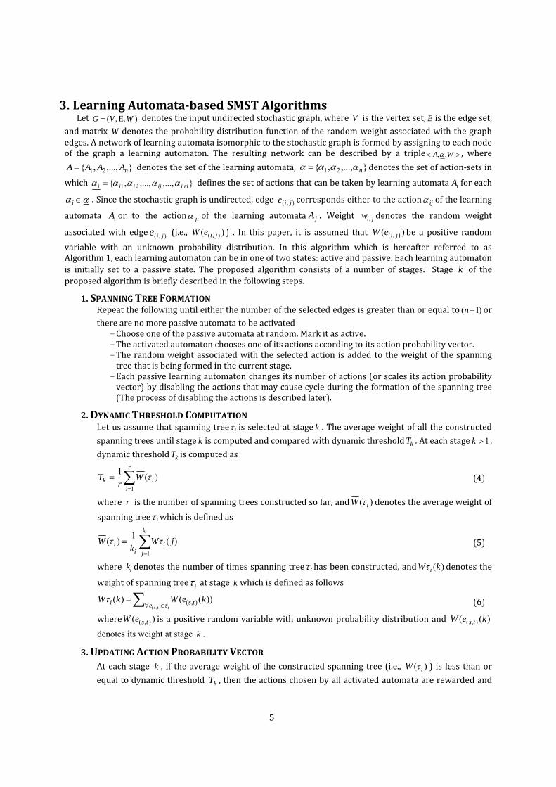
3. Learning Automatabased SMST Algorithms Let ),Ε,(= WVG denotes the input undirected stochastic graph, where V is the vertex set, E is the edge set,
and matrix W denotes the probability distribution function of the random weight associated with the graph edges. A network of learning automata isomorphic to the stochastic graph is formed by assigning to each node of the graph a learning automaton. The resulting network can be described by a triple >< WA ,,α , where
},...,,{ 21 nAAAA = denotes the set of the learning automata, },...,,{ 21 nαααα = denotes the set of action‐sets in
which },...,,...,,{ 21 riiijiii ααααα = defines the set of actions that can be taken by learning automata iA for each
αα ∈i . Since the stochastic graph is undirected, edge ),( jie corresponds either to the action ijα of the learning
automata iA or to the action jiα of the learning automata jA . Weight jiw , denotes the random weight
associated with edge ),( jie (i.e., )( ),( jieW ) . In this paper, it is assumed that )( ),( jieW be a positive random variable with an unknown probability distribution. In this algorithm which is hereafter referred to as Algorithm 1, each learning automaton can be in one of two states: active and passive. Each learning automaton is initially set to a passive state. The proposed algorithm consists of a number of stages. Stage k of the proposed algorithm is briefly described in the following steps.
1. SPANNING TREE FORMATION Repeat the following until either the number of the selected edges is greater than or equal to )1( −n or there are no more passive automata to be activated
- Choose one of the passive automata at random. Mark it as active. - The activated automaton chooses one of its actions according to its action probability vector. - The random weight associated with the selected action is added to the weight of the spanning tree that is being formed in the current stage.
- Each passive learning automaton changes its number of actions (or scales its action probability vector) by disabling the actions that may cause cycle during the formation of the spanning tree (The process of disabling the actions is described later).
2. DYNAMIC THRESHOLD COMPUTATION Let us assume that spanning tree iτ is selected at stage k . The average weight of all the constructed spanning trees until stage k is computed and compared with dynamic threshold kT . At each stage 1>k , dynamic threshold kT is computed as
(4) ∑=
=r
iik W
rT
1
)(1 τ
where r is the number of spanning trees constructed so far, and )( iW τ denotes the average weight of spanning tree iτ which is defined as
(5) ∑=
=ik
ji
ii jW
kW
1
)(1)( ττ
where ik denotes the number of times spanning tree iτ has been constructed, and )(kW iτ denotes the
weight of spanning tree iτ at stage k which is defined as follows
(6) ∑ ∈∀=
itse tsi keWkWτ
τ),(
))(()( ),( where )( ),( tseW is a positive random variable with unknown probability distribution and )(( ),( keW ts
denotes its weight at stage k .
3. UPDATING ACTION PROBABILITY VECTOR At each stage k , if the average weight of the constructed spanning tree (i.e., )( iW τ ) is less than or equal to dynamic threshold kT , then the actions chosen by all activated automata are rewarded and
6
penalized otherwise. In this algorithm, each automaton updates its action probability vector by using a IRL − reinforcement scheme. The disabled actions are enabled again and the probability vectors are updated as described in Subsection 2.3.
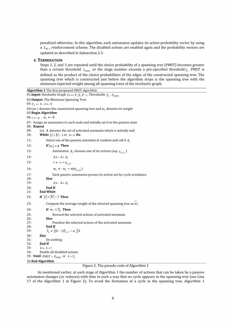
4. TERMINATION Steps 1, 2, and 3 are repeated until the choice probability of a spanning tree (PMST) becomes greater than a certain threshold PMSTT or the stage number exceeds a pre‐specified threshold kT . PMST is defined as the product of the choice probabilities of the edges of the constructed spanning tree. The spanning tree which is constructed just before the algorithm stops is the spanning tree with the minimum expected weight among all spanning trees of the stochastic graph.
Algorithm 1 The first proposed SMST algorithm01:Input: Stochastic Graph >=< FEVG ,, , Thresholds kT , PMSTT
02:Output: The Minimum Spanning Tree 03: 0←kT , 0←k 04:Let denotes the constructed spanning tree and denotes its weight 05:Begin Algorithm 06: ϕτ ← , 0←τw 07: Assign an automaton to each node and initially set it to the passive state 08: Repeat 09: Let A denotes the set of activated automata which is initially null 10: While 1−< Vτ or nA < Do 11: Select one of the passive automata at random and call it iA 12: If φα ≠i Then 13: Automaton iA chooses one of its actions (say ),( jie )
14: iAAA +← 15: ),( jie+←ττ
16: )( ),( jiewww +← ττ
17: Each passive automaton prunes its action‐set for cycle avoidance 18: Else 19: iAAA +← 20: End If 21: End While
22: If 1−= Vτ Then
23: Compute the average weight of the selected spanning tree as τw
24: If kTw ≤τ Then 25: Reward the selected actions of activated automata 26: Else 27: Penalize the selected actions of the activated automata 28: End If 29: [ ] kwTkT kk τ+−← −1)1( 30: Else 31: Do nothing 32: End If 33: 1+← kk 34: Enable all disabled actions 35: Until PMSTPPMST > or kTk > 36:End Algorithm
Figure 2. The pseudo code of Algorithm 1
As mentioned earlier, at each stage of Algorithm 1 the number of actions that can be taken by a passive automaton changes (or reduces) with time in such a way that no cycle appears in the spanning tree (see Line 17 of the Algorithm 1 in Figure 2). To avoid the formation of a cycle in the spanning tree, Algorithm 1
7
performs as follows: Let ji,π denotes the path connecting node iv to node jv , and ijp and i
jq denote the
choice probability of edge ) ,( jie and path ji,π , respectively. Now, at each stage k , the proposed algorithm
removes every edge )s ,(re (or ) ,( rse ) and temporarily disables its corresponding action in the action‐set of the
passive automata rA and sA , if edge ) ,( jie is chosen at stage k and both paths ri,π and sj,π
has been already
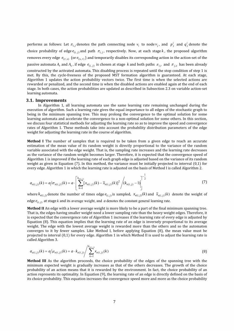
constructed by the activated automata. This disabling process is repeated until the stop condition of step 1 is met. By this, the cycle‐freeness of the proposed MST formation algorithm is guaranteed. At each stage, Algorithm 1 updates the action probability vectors twice. The first time is when the selected actions are rewarded or penalized, and the second time is when the disabled actions are enabled again at the end of each stage. In both cases, the action probabilities are updated as described in Subsection 2.3 on variable action‐set learning automata.
3.1. Improvements In Algorithm 1, all learning automata use the same learning rate remaining unchanged during the
execution of algorithm. Such a learning rate gives the equal importance to all edges of the stochastic graph to being in the minimum spanning tree. This may prolong the convergence to the optimal solution for some learning automata and accelerate the convergence to a non‐optimal solution for some others. In this section, we discuss four statistical methods for adjusting the learning rate so as to improve the speed and convergence rates of Algorithm 1. These methods take into account the probability distribution parameters of the edge weight for adjusting the learning rate in the course of algorithm. Method I The number of samples that is required to be taken from a given edge to reach an accurate estimation of the mean value of its random weight is directly proportional to the variance of the random variable associated with the edge weight. That is, the sampling rate increases and the learning rate decreases as the variance of the random weight becomes larger. Therefore, it is expected that the convergence speed of Algorithm 1 is improved if the learning rate of each graph edge is adjusted based on the variance of its random weight as given in Equation (7). In this method, the variance must be initially projected to interval 0,1 for every edge. Algorithm 1 in which the learning rate is adjusted on the basis of Method I is called Algorithm 2.
(7) 21
),(1
2),(),(),(),( )1()]()([)()(
),(−
= ⎥⎥⎦
⎤
⎢⎢⎣
⎡−−⋅== ∑ jie
k
kjiejiejiejie kkxkxakaka
jie
σ
where ),( jiek denote the number of times edge ),( jie is sampled, )(),( kx jie and )(),( kx jie denote the weight of
edge ),( jie at stage k and its average weight, and a denotes the constant general learning rate.
Method II An edge with a lower average weight is more likely to be a part of the final minimum spanning tree. That is, the edges having smaller weight need a lower sampling rate than the heavy weight edges. Therefore, it is expected that the convergence rate of Algorithm 1 increases if the learning rate of every edge is adjusted by Equation (8). This equation implies that the learning rate of an edge is inversely proportional to its average weight. The edge with the lowest average weight is rewarded more than the others and so the automaton converges to it by fewer samples. Like Method I, before applying Equation (8), the mean value must be projected to interval 0,1 for every edge. Algorithm 1 in which Method II is used to adjust the learning rate is called Algorithm 3.
(8) ∑=
⋅==),(
1),(),(),(),( )()()(
jiek
kjiejiejiejie kxkakaka µ
Method III As the algorithm proceeds, the choice probability of the edges of the spanning tree with the minimum expected weight is gradually increases as that of the others decreases. The growth of the choice probability of an action means that it is rewarded by the environment. In fact, the choice probability of an action represents its optimality. In Equation (9), the learning rate of an edge is directly defined on the basis of its choice probability. This equation increases the convergence speed more and more as the choice probability
8
increases (or as the algorithm approaches to the end). Algorithm 1 in which the learning rate is computed by Equation (9) is called Algorithm 4.
(9) )()( ),(),( kPaka jiejie ⋅=
Method IV Equation (8) can be used in applications that sacrifice the running time in favor of the solution optimality, while Equation (9) is appropriate for applications that give significant importance to the running time. Different combinations of the previous methods (Methods I‐III) can be also used for applications in which a trade‐off between the running time and solution optimality is desired. We combined Method II and Method III in order to improve both the convergence rate and convergence speed of Algorithm 1. This method is called Method IV and computes the learning rate as given in Equation (10). Algorithm 1 in which Method IV is used to adjust the learning rate is called Algorithm 5.
(10) ∑=
⋅⋅=⋅
=),(
1),(),(),(
),(
),(),( )()(
)()(
)(jiek
kjiejiejie
jie
jiejie kxkkPa
kkPa
kaµ
4. Convergence Results In this section we prove two main results of the paper. The first result concerns the convergence of
Algorithm 1 to the optimal solution when each learning automaton updates its action‐set by a linear reward‐inaction reinforcement scheme (Theorem 1). This result represents that by choosing a proper learning rate for Algorithm 1, the choice probability of the optimal solution converges to one as much as possible. Since Algorithm 1 is designed for stochastic environments where the environmental parameters vary over time, the method that is used to prove the convergence of the Algorithm 1 partially follows the method given in [12, 13] to analyze the behavior of the learning automata operating in non‐stationary environments. The second result concerns the relationship between the convergence error parameter ε (i.e. the error parameter involves in the standard sampling method) and the learning rate of the Algorithm 1 (Theorem 3). The second result aims at determining a learning rate )(εa under which the probability of constructing the spanning tree with the minimum expected weight exceeds ε−1 .
Theorem 1 Let )(kqi be the probability of constructing spanning tree iτ at stage k . If )(kq is updated according
to Algorithm 1, then there exists a learning rate )1,0()(* ∈εa (for every 0>ε ) such that for all ),0( *aa∈ , we have
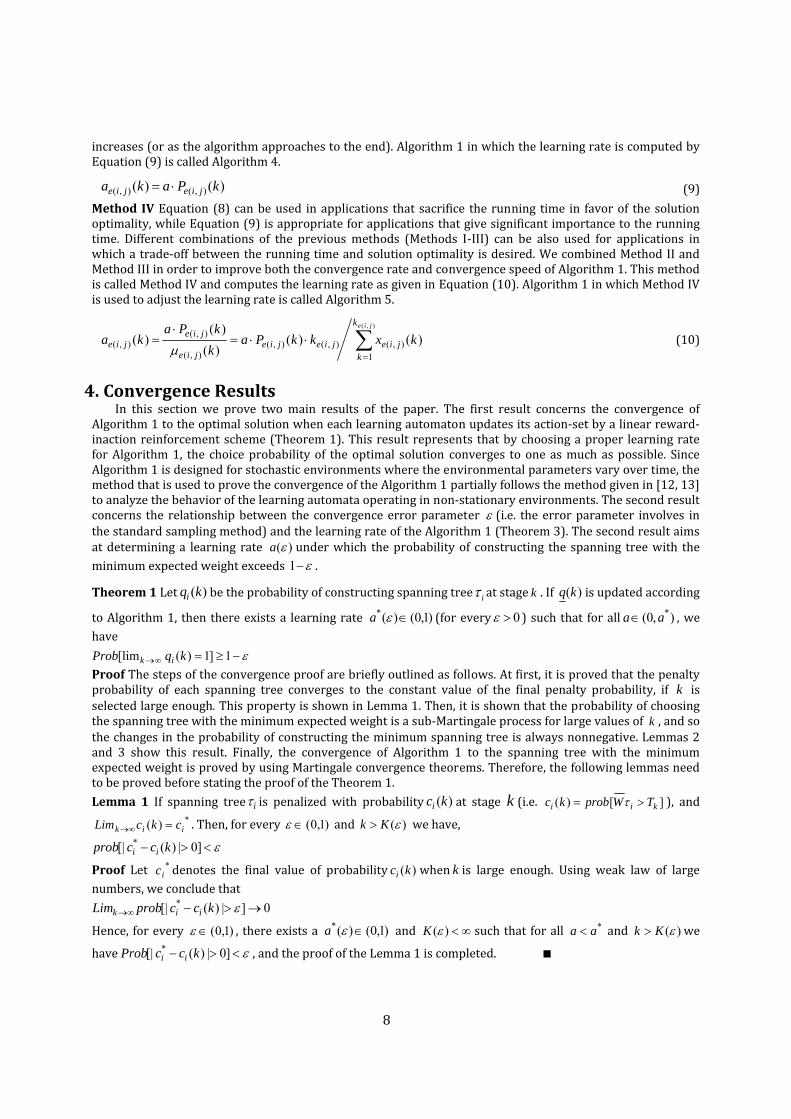
ε−≥=∞→ 1]1)([lim kqProb ik Proof The steps of the convergence proof are briefly outlined as follows. At first, it is proved that the penalty probability of each spanning tree converges to the constant value of the final penalty probability, if k is selected large enough. This property is shown in Lemma 1. Then, it is shown that the probability of choosing the spanning tree with the minimum expected weight is a sub‐Martingale process for large values of k , and so the changes in the probability of constructing the minimum spanning tree is always nonnegative. Lemmas 2 and 3 show this result. Finally, the convergence of Algorithm 1 to the spanning tree with the minimum expected weight is proved by using Martingale convergence theorems. Therefore, the following lemmas need to be proved before stating the proof of the Theorem 1. Lemma 1 If spanning tree iτ is penalized with probability )(kci at stage k (i.e. ][)( kii TWprobkc >= τ ), and
*)( iik ckcLim =∞→ . Then, for every )1,0(∈ε and )(εKk > we have, ε<>− ]0|)([| * kccprob ii
Proof Let *ic denotes the final value of probability )(kci when k is large enough. Using weak law of large
numbers, we conclude that 0]|)([| * →>−∞→ εkccprobLim iik
Hence, for every )1,0(∈ε , there exists a )1,0()(* ∈εa and ∞<)(εK such that for all *aa < and )(εKk > we
have ε<>− ]0|)([| * kccProb ii , and the proof of the Lemma 1 is completed. ■
9
Lemma 2 Let ])1([)( kjj TkWprobkc >+= τ and )(1)( kckd jj −= be the probability of penalizing and
rewarding spanning tree jτ (for all rj ,...,2,1= ) at stage k , respectively. If )(kq evolves according to Algorithm
1, then the conditional expectation of )(kqi is defined as
∑ ∏= ∈
+=+r
j nme
mnjijji
i
kdkqkckqkqkqE1 ),(
])()()()[()](|)1([τ
δ
where
⎪⎩
⎪⎨⎧
∉−⋅=+
∈−+=+=
jnmmn
mn
jnmmn
mn
mnm
neakpkp
ekpakpkpk
τ
τδ
),(
),(
;)1()()1(
;))(1()()1()(
where r denotes all constructed spanning trees. Proof Since the reinforcement scheme that is used to update the probability vectors in Algorithm 1 is IRL − , at each stage k the probability of choosing the spanning tree iτ (i.e., )(kqi ), remains unchanged with probability
)(kc j (for all rj ,...,2,1= ), when the selected spanning tree jτ is penalized by the random environment. On the
other hand, when the selected spanning tree jτ is rewarded, the probability of choosing the edges of the
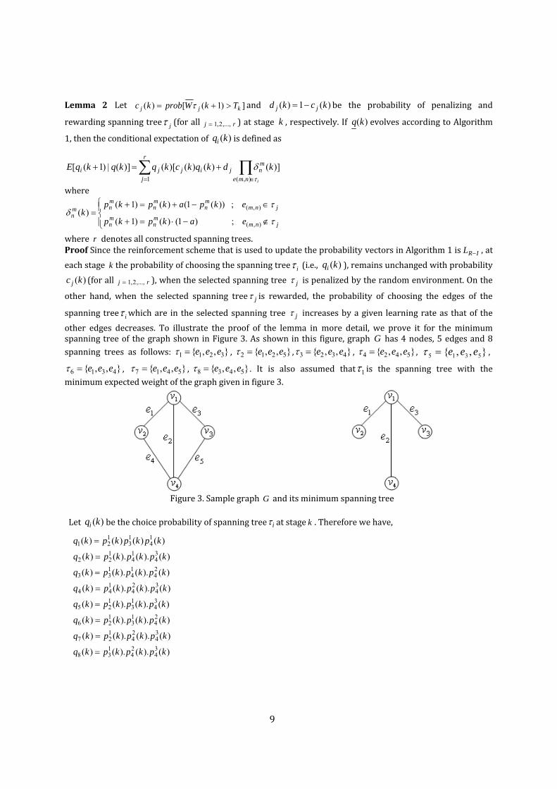
spanning tree iτ which are in the selected spanning tree jτ increases by a given learning rate as that of the other edges decreases. To illustrate the proof of the lemma in more detail, we prove it for the minimum spanning tree of the graph shown in Figure 3. As shown in this figure, graph G has 4 nodes, 5 edges and 8 spanning trees as follows: },,{ 3211 eee=τ , },,{ 5212 eee=τ , },,{ 4323 eee=τ , },,{ 5424 eee=τ , },,{ 5315 eee=τ ,
},,{ 4316 eee=τ , },,{ 5417 eee=τ , },,{ 5438 eee=τ . It is also assumed that 1τ is the spanning tree with the minimum expected weight of the graph given in figure 3.
Figure 3. Sample graph G and its minimum spanning tree
Let )(kqi be the choice probability of spanning tree iτ at stage k . Therefore we have,
)().().()(
)().().()(
)().().()(
)().().()(
)().().()(
)().().()(
)().().()(
)()()()(
34
24
138
34
24
127
24
13
126
34
13
125
34
24
144
24
14
133
34
14
122
14
13
121
kpkpkpkq
kpkpkpkq
kpkpkpkq
kpkpkpkq
kpkpkpkq
kpkpkpkq
kpkpkpkq
kpkpkpkq
=
=
=
=
=
=
=
=
10
where )(kpij denotes the probability of choosing action ijα of automaton iA at stage k. The conditional
expectation of )1(1 +kq , assuming )(kq is updated according to Algorithm 1, is defined as
[ ][ ][ ][ ][ ][ ][ ][ ])}1)(())}{(1()()}{1)((){()()(
)}1)(()}{1)(())}{(1()(){()()(
)}1)(())}{(1()())}{(1()(){()()(
)}1)(())}{(1()())}{(1()(){()()(
))}(1()()}{1)(()}{1)((){()()(
))}(1()())}{(1()()}{1)((){()()(
))}(1()()}{1)(())}{(1()(){()()(
))}(1()())}{(1()())}{(1()(){()()(
)](|)1([
14
13
13
128188
14
13
12
127177
14
13
13
12
126166
14
13
13
12
125155
14
14
13
124144
14
14
13
13
123133
14
14
13
12
122122
14
14
13
13
12
121111
1
akpkpakpakpkdkqckq
akpakpkpakpkdkqckq
akpkpakpkpakpkdkqckq
akpkpakpkpakpkdkqckq
kpakpakpakpkdkqckq
kpakpkpakpakpkdkqckq
kpakpakpkpakpkdkqckq
kpakpkpakpkpakpkdkqckq
kqkqE
−−+−+
+−−−++
+−−+−++
+−−+−++
+−+−−+
+−+−+−+
+−+−−++
+−+−+−++
=+
After simplifying all terms in the right hand side of the equation above and some algebraic manipulations, we obtain
⎪⎩
⎪⎨⎧
∉−⋅=+
∈−+=+=
+=+ ∑ ∏= ∈
jnmmn
mn
jnmmn
mn
mnm
n
j nme
mnjjj
eakpkp
ekpakpkpk
kkdkqkckqkqkqE
τ
τδ
δτ
),(
),(
8
1 ),(11
;)1()()1(
;))(1()()1()(
])()()()()[()](|)1([1
and hence the proof of the lemma. ■ Lemma 3 The increment in the conditional expectation of )(kqi is always non‐negative subject to )(kq is
updated according to Algorithm 1. That is, 0)( >∆ kqi .
Proof. Define )()](|)1([)( kqkqkqEkq iii −+=∆ .
From Lemma 2, we have
(11)
)(])()()()[()()](|)1([)(1 ),(
kqkdkqkckqkqkqkqEkq i
r
j nme
mnjijjiii
i
−+=−+=∆ ∑ ∏= ∈τ
δ
where
⎪⎩
⎪⎨⎧
∉−⋅=+
∈−+=+=
jnmmn
mn
jnmmn
mn
mnm
neakpkp
ekpakpkpk
τ
τδ
),(
),(
;)1()()1(
;))(1()()1()(
where )(kpmn is the probability of choosing edge ),( nme
at stage k . Since the probability with which the
spanning trees are constructed, rewarded or penalized is defined as the product of the probability of choosing the edges along the spanning trees, we have
∏
∑ ∏∏∏∏∏
∈
= ∈∈∈∈∈
−
⎥⎥
⎦
⎤
⎢⎢
⎣
⎡⋅+⋅=∆
i
ijijj
nme
mn
r
j nme
mn
nme
mn
nme
mn
nme
mn
nme
mni
kp
kkdkpkckpkq
τ
τττττ
δ
),(
1 ),(),(),(),(),(
)(
)()()()()()(
where )(kmnδ is defined as given in Equation (11) and )(kcm
n is the probability of penalizing edge ),( nme at stage
k and )(1)( kckd mn
mn −= . At each stage, Algorithm 1 exactly chooses )1( −n edges of the stochastic graph
forming one of r possible spanning trees.
11
[ ] ∏∏∈∈
−+=∆ii nme
mn
nme
mmni kpkpkpEkq
ττ ),(),(
)()(|)1()(
The equality above can be rewritten as
(12) [ ] ∏∏∈∈
∆=−+≥∆ii nme
mn
mn
nme
mmni kpkpkpkpEkq
ττ ),(),(
)())()(|)1(()(
and
∑≠
−⋅⋅=∆mr
ns
mn
ms
ms
mn
mn kckckpkpakp ))()(()()()(
)1,0()( ∈kqi for all 0rSq ∈ , where }1)(;1)(0:)({
1=≤≤= ∑ =
r
i iir kqkqkqS and 0rS denotes the interior of rS .
Hence, )1,0()( ∈kpmn for all nm, . Since edge inme τ∈),(
is the edge with the minimum expected weight which
can be selected by automaton mA , it is shown that 0**
>− mn
ms cc for all ns ≠ . It follows from Lemma 1 that for
large values of k , 0)()( >− kckc mn
ms . Therefore, we conclude that for large values of k , the right hand side of
the equation above consists of the nonnegative quantities and so we have
0))()(()()(),(
≥−⋅⋅∏ ∑∈ ≠i
m
nme
r
ns
mn
ms
ms
mn kckckpkpa
τ
and from Equation (12),we have
∏ ∑∈ ≠
−⋅⋅≥∆i
m
nme
r
ns
mn
ms
ms
mni kckckpkpakq
τ),(
))()(()()()(
which completes the proof of this lemma. ■ Corollary 1 The set of unit vectors in 0
rr SS − forms the set of all absorbing barriers of the Markov process
1)}({ ≥kkq , where }1)();1,0()(:)({1
0 =∈= ∑ =
r
i iir kqkqkqS
Proof Lemma 3 implicitly proves that )}({ kq is a sub‐Martingale. Using Martingale theorems and the fact that
)}({ kq is a non‐negative and uniformly bounded function, it is concluded that )(kqLim ik ∞→ converges to *q with probability one. Hence, from Equation (11), it can be seen that )()1( kqkq ii ≠+ with a nonzero probability
if and only if }1,0{)( ∉kqi , and )()1( kqkq =+ with probability one if and only if }1,0{* ∈q where*)( qkqLim ik =∞→ , and hence the proof is completed. ■
Let )(qiΓ be the probability of convergence of Algorithm 1 to unit vector ie with initial probability vector q . )(qiΓ is defined as follows
])0(|[])0(|1)([)( qqeqprobqqqprobq iii =====∞=Γ ∗ Let ℜ→rr SSC :)( be the state space of all real‐valued continuously differentiable functions with
bounded derivative defined on rS , whereℜ is the real line. If )((.) rSC∈ψ , the operatorU is defined as
(13) ])(|)1(([)( qkqkqEqU =+= ψψ where [.]E represents the mathematical expectation.
12
It has been shown in [13] that operatorU is linear, and it preserves the non‐negative functions as the expectation of a nonnegative function remains nonnegative. In other word, 0)( ≥qUψ for all rSq∈ , if 0)( ≥qψ. If the operatorU is applied n (for all 1>n ) times repeatedly, we have
])1(|)1(([)(1 qqkqEqU n =+=− ψψ Function )(qψ is called super‐regular (sub‐regular) if and only if )()( qUq ψψ ≥ ( ))()( qUq ψψ ≤ , for all
rSq∈ . It has been shown in [13] that )(qiΓ is the only continuous solution of )()( qqU ii Γ=Γ subject to the following boundary conditions.
(14) ijee
ji
ii
≠=Γ=Γ
;0)(1)( Define
1
1],[−
−= −
−
ai x
aixq
e
eqxφ
where 0>x . )(],[ ri SCqx ∈φ satisfies the boundary conditions above.
Theorem 2 Let )((.) ri SC∈ψ be super‐regular with 1)( =ii eψ and 0)( =ji eψ for ij ≠ , then
)()( qq ii Γ≥ψ for all rSq∈ . If )((.) ri SC∈ψ is sub‐regular with the same boundary conditions, then
(15) )()( qq ii Γ≤ψ for all rSq∈ . Proof. Theorem 2 has been proved in [12]. ■
In what follows, we show that ],[ qxiφ is a sub‐regular function, and ],[ qxiφ qualifies as a lower bound on )(qiΓ . Super and sub‐regular functions are closed under addition and multiplication by a positive constant, and if (.)φ is super‐regular then (.)φ− is sub‐regular. Therefore, it follows that ],[ qxiφ is sub‐regular if and only if
aixq
eqxi
−
=],[θ is super‐regular. We now determine the conditions under which ],[ qxiθ is super‐regular. From the definition of operator Ugiven in Equation (13), we have
⎥⎥⎥⎥
⎦
⎤
⎢⎢⎢⎢
⎣
⎡
++=
⎥⎥⎥⎥
⎦
⎤
⎢⎢⎢⎢
⎣
⎡
+=⎥⎥⎦
⎤
⎢⎢⎣
⎡==
∑∑
∑∑
≠
−−
≠
−+−−+−
=
−−
=
−+−+
−
∏∏
∏∏
∉∈
∈∈
∉∈
∈∈
ij
apax
jjij
papax
jjqaq
ax
ii
r
j
apax
jj
r
j
papax
jjakxq
i
jnmeinme
mn
jnmeinme
mn
mn
ii
jnmeinme
mn
jnmeinme
mn
mn
i
edqedqedq
edqedqqkqeEqxU
]))1(([
*
]))1(([
*))1((*
1
]))1(([
*
1
]))1(([
*)1(
),(,),(
),(,),(
),(,),(
),(,),(
)(),(
ττ
ττ
ττ
ττ
θ
13
where *jd denotes the final value to which the reward probability )(kd j is converged (for large values of k ),
and ))1(( ii qaq
ax
e−+−
is the expectation of ),( qxiθ when the minimum spanning tree iτ is rewarded by the environment .
⎥⎥⎦
⎤
⎢⎢⎣
⎡+=
⎥⎥⎥⎥⎥⎥
⎦
⎤
⎢⎢⎢⎢⎢⎢
⎣
⎡
+=
∑∑
∑
≠
−−
=
−+−
≠
⎟⎟⎟⎟
⎠
⎞
⎜⎜⎜⎜
⎝
⎛
−−+
⋅−−
−+−∏
∈∈
ij
aqax
jjij
qaqax
jj
ij
appapaq
ax
jjqaq
ax
iii
iijii
ij
jnmeinme
mn
mn
mn
i
ii
edqedq
edqedqqxU
))1((*))1((*
))1(())1(()1(
*))1((* ),(,),(
),(
ρρ
ττ
θ
where 0>ijρ
is defined as
⎪⎪⎩
⎪⎪⎨
⎧
=∩=
≠∏−
−+
= ∈∈
φττ
ρ ττ
)(;1
;))1((
))1((
),(,),(
ji
nmenme m
n
mn
mn
ij
orji
jiappap
ji
axq
xq
ijjj
axq
ij
qxjj
axq
ii
iiji
iji
iji
iji
eedqeedqeqxqxU−
≠
−
=
−−−−
⎥⎥⎥
⎦
⎤
⎢⎢⎢
⎣
⎡+=− ∑∑ ρ
ρρ
ρ
θθ *)1(*),(),(
),( qxiθ is super‐regular if
axq
xq
ijjj
axq
ij
qxjj
axq ii
ji
iji
iji
iji
eedqeedqe−
≠
−
=
−−−≤+ ∑∑ ρ
ρρ
ρ*)1(*
and
i
i
i
ixq
ijjj
axq
qxii
axq
i edqeedqeqxU ∑≠
−−−−+≤ *)1(*),(θ
If ),( qxiθ is super‐regular. Therefore, we have
axq
xq
ijjj
axq
qxii
axq
ii
i
i
i
i
i
eedqeedqeqxqxU−
≠
−−−−−
⎥⎥⎦
⎤
⎢⎢⎣
⎡+≤− ∑ *)1(*),(),( θθ
After multiplying and dividing the right hand side of the inequality above by ixq− and some algebraic simplifications, we have
14
⎥⎥⎦
⎤
⎢⎢⎣
⎡ −−
−−−
−−=
⎥⎥⎦
⎤
⎢⎢⎣
⎡ −−
−−
−=
⎥⎥⎦
⎤
⎢⎢⎣
⎡ −−
−−
−≤−
∑
∑
∑
≠
−−
≠
−−
≠
−−
−
−
−
i
xq
ijjj
i
qx
iii
i
xq
ijjj
qx
ii
i
xq
ijjj
i
qx
iiiii
xqedq
qxedqexq
xqedq
xedexq
xqedq
xqedqexqqxqxU
ii
ii
ii
aixq
aixq
aixq
1)1(1)1(
11
11),(),(
*)1(
*
*)1(
*
*)1(
*θθ
and
⎪⎩
⎪⎨
⎧
=
≠−
=0;1
0;1][
u
uu
euV
u
),(),(
][)()]1([)1(),(),( **
qxGqxxq
xqVdqqxVdqexqqxqxU
iii
iij
jjiiiiiia
ixq
θ
θθ
−=
⎥⎥⎦
⎤
⎢⎢⎣
⎡−−−−−≤− ∑
≠
−
where ),( qxGi is defined as
(16) ][)()]1([)1(),( **iij jjiiii xqVdqqxVdqqxG ∑ ≠
−−−−= Therefore, ),( qxiθ is super‐regular if
(17) 0),( ≥qxGi for all rSq∈ .
From Equation (16), it follows that ),( qxiθ is super‐regular if we have
(18) *
*
)1(][)]1([),(
ii
ij jj
i
ii dq
dq
xqVqxVqxf
−≤
−−=
∑ ≠ The right hand side of the inequality (18) consists of the nonnegative terms, so we have
⎟⎟
⎠
⎞
⎜⎜
⎝
⎛⎟⎠⎞⎜
⎝⎛≤
−≤
⎟⎟
⎠
⎞
⎜⎜
⎝
⎛⎟⎠⎞⎜
⎝⎛
≠≠≠≠≠ ∑∑∑ *
*
*
*
*
*
max)1(
1mini
j
ijij ji
jij j
ii
j
ijij j d
dq
d
dq
qd
dq
Substituting ∑ ≠ij jq by )1( iq− in the above inequality, we can rewrite it as
⎟⎟
⎠
⎞
⎜⎜
⎝
⎛≤≤
⎟⎟
⎠
⎞
⎜⎜
⎝
⎛
≠≠
≠
≠ ∑∑
*
**
*
*
*
maxmini
j
ijij j
i
jij j
i
j
ij d
d
qd
dq
d
d
From Equation (18), it follows that ),( qxiθ is super‐regular if we have
( )**max),( ijij
i ddqxf≠
≥ For further simplification, let employ logarithms. Let
),(ln),( qxfxq i=∆
It has been shown in [13] that
15
)(ln)(,)()(
)(),()(0
0
uVuHdu
udHuH
duuHxqduuHx
x
==
′−≤∆≤′− ∫∫ −
Therefore, we have
][][
)]1([][
1 xVxqV
qxVxV i
i −≤−−
≤ and
(19) ⎟⎟
⎠
⎞
⎜⎜
⎝
⎛=
≠ *
*
max][
1
i
j
ij d
dxV
Let *x be the value of x for which Equation (19) is true. It is shown that there exists a value of 0>x under which the Equation (19) is satisfied, if )( ij dd is smaller than 1 for all ij ≠ . By choosing *xx = Equation (19) holds true. Consequently, Equation (17) is true and ),( qxiθ is a super‐regular function. Therefore,
1
1],[−
−= −
−
ai x
aixq
e
eqxφ
is a sub‐regular function satisfying the boundary conditions given in Equation (14). From Theorem 2 and Inequality (15), we conclude that
1)(],[ ≤Γ≤ qqx iiφ From definition of ],[ qxiφ , we see that given any 0>ε there exists a positive constant 1* <a such that
1)(],[1 ≤Γ≤≤− qqx iiφε for all *0 aa ≤< .
Thus we conclude that the probability with which Algorithm 1 constructs the spanning tree with the minimum expected weight is equal to 1 as k converges to infinity, and so Theorem 1 is proved. ■ Theorem 3 Let )(kqi be the probability of constructing minimum spanning tree iτ at stage k , and )1( ε− be the
probability with which Algorithm 1 converges to spanning tree iτ . If )(kq is updated by Algorithm 1, then for
every error parameter )1,0(∈ε there exists a learning rate ),( qa ε∈ so that
⎟⎟⎠
⎞⎜⎜⎝
⎛=
−≠
i
jijxa d
d
exa max
1
where )1()1(1 ε−⋅−=− −− xxq ee i and ]0|)([ == kkqq ii .
Proof It has been proved in [13, 17] that there always exists a 0>x under which Equation (19) is satisfied, if 1<ij dd for all ij ≠ . Hence, it is concluded that
x
xq
ii eeqqx
i
−
−
−−
≤Γ≤1
1)(],[φ where iq is the initial choice probability of the optimal spanning tree iτ . From Theorem 1, we have for each
*0 aa << the probability of converging Algorithm 1 to the spanning tree with the minimum expected weight is )1( ε− where )1,0()(* ∈εa . Therefore, we conclude that
(20) ε−=−
−−
−
11
1x
xq
ee i
16
It is shown that for every error parameter )1,0(∈ε there exists a value of x under which Equation (19) is satisfied, and so we have
⎟⎟
⎠
⎞
⎜⎜
⎝
⎛=
− ≠ *
*
*
*max
1 i
j
ijax d
d
eax
It is concluded that for every error parameter )1,0(∈ε there exists a learning rate ),( qa ε∈ under which the probability of converging Algorithm 1 to the spanning tree with the minimum expected weight is greater than )1( ε− and hence the proof of the theorem. ■
5. Numerical Results To study the efficiency of the proposed algorithms, we have conducted three set of simulation
experiments on four well‐known stochastic benchmark graphs borrowed from [41, 42]. The first set of experiments aims to investigate the relationship between the learning rate of Algorithm 1 and the error rate in standard sampling method. These experiments show that for every error rate , there exists a learning rate such that for algorithm 1 construct the spanning tree with the minimum expected weight. This set
of experiment is conducted on stochastic graphs Alex2‐B and Alex3‐B [41]. The second set of simulation experiments compare the performance of the SMST algorithms proposed in this paper (Algorithm 1 to Algorithm 5). These experiments are conducted on Alex2‐B and Alex3‐B too. The third set of experiments aims to show the efficiency of Algorithm 5 which is the best proposed algorithm in comparison with MESM (multiple edge sensitivity method)[41]. In all three set of experiments conducted in this paper, the reinforcement scheme by which the action probability vector is updated is IRL − . Each algorithm stops if the probability of the constructed spanning tree (PMST) is equal to or greater than 0.95 or the number of constructed spanning trees exceeds a pre‐defined threshold 100,000. For each experiment, the results are averaged over 100 different independent runs.
5.1. Experiment I This set of experiments is conducted on two sparse graphs called Alex2 and Alex3. Alex2 comprises 9
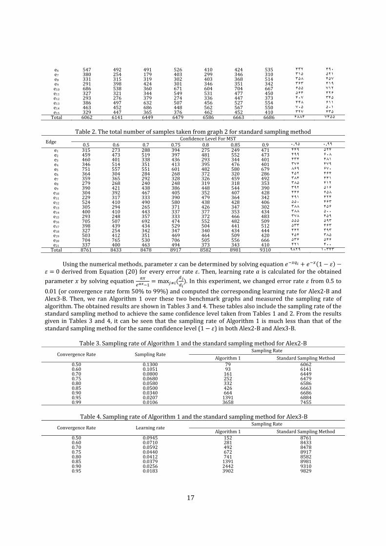
nodes and 15 edges, and Alex3 has 10 nodes and 21 edges. The discrete random variable associated with the edge weight of Alex2 and Alex3 has two and three states in mode A and B, respectively. The probability distribution of the random weight assigned to the edges of Alex2 and Alex3 tends toward the smaller edge weights. In other words, the higher probabilities are assigned to the edges with smaller weights. Such a biased distribution is more pragmatic for modeling the network dynamics than a simple uniform distribution. The first set of experiment compares the efficiency of Algorithm 1 with the standard sampling method in terms of the sampling rate. To do so, by Theorem 3, the learning rate corresponding to each confidence level 1 in initially computed (see Tables 1 and 2). Then, Algorithm 1 is run with the obtained learning rate and its sampling rate is measured. Finally, the sampling rate of Algorithm 1 is compared with that of the standard sampling method to obtain the same confidence level.
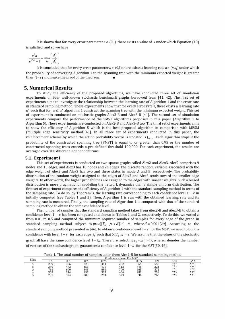
The number of samples that the standard sampling method takes from Alex2‐B and Alex3‐B to obtain a confidence level 1 has been computed and shown in Tables 1 and 2, respectively. To do this, we varied from 0.01 to 0.5 and computed the minimum required number of samples for every edge of the graph in standard sampling method subject to εδµ −≥<− 1]|[| nxprob , where 001.0=δ [29]. According to the standard sampling method presented in [46], to obtain a confidence level ε−1 for the MST, we need to build a confidence with level iε−1 for each edge ie such that ∑ . We assume that the edges of the stochastic graph all have the same confidence level 01 ε− . Therefore, selecting )1(0 −= nεε , where n denotes the number of vertices of the stochastic graph, guarantees a confidence level ε−1 for the MST[30, 46].
Table 1. The total number of samples taken from Alex2‐B for standard sampling method Edge Confidence Level For MST
0.5 0.6 0.7 0.75 0.8 0.85 0.9 ٠٫٩۵ ٠٫٩٩ e1 299 366 323 314 282 365 555 ۴٣۴ ۴٧٢ e2 359 473 451 475 412 345 324 ۴٣٨ ٩٩۴ e3 761 600 843 694 700 665 572 ۶٧ ١١۶٧ e4 307 314 357 337 404 282 259 ٣٢٩ ۴۵٧ e5 295 394 289 294 373 336 265 ۴٢٩ ۴۵٠
17
e6 547 492 491 526 410 424 535 ۴٣٢ ۴٩٠ e7 380 254 179 403 299 346 310 ٣١۵ ۵٢١ e8 331 315 319 302 403 368 514 ٣۵٨ ۴۵٧ e9 291 398 424 301 346 351 342 ٣۶٣ ۴١٩ e10 686 538 360 671 604 704 667 ۶۵۵ ٧١٢ e11 327 321 344 549 531 477 450 ۵۶۴ ۴٢۶ e12 293 276 379 274 336 447 373 ۴٣ ٠٧۴۵ e13 386 497 632 507 456 527 554 ۴۴٨ ۶١١ e14 463 452 686 448 562 567 550 ٧٠۵ ۵٠١ e15 329 447 365 376 462 452 410 ٣٢٧ ۴٣۵ Total 6062 6141 6449 6479 6586 6663 6686 ۶٨٨۴ ٧۴۵۵
Table 2. The total number of samples taken from graph 2 for standard sampling method Edge Confidence Level For MST
0.5 0.6 0.7 0.75 0.8 0.85 0.9 ٠٫٩۵ ٠٫٩٩ e1 315 273 288 394 275 249 471 ۴۴٩ ۵٢۴ e2 459 473 519 397 481 552 473 ۴٩٩ ۶٠٨ e3 460 401 338 436 293 344 401 ۴٣۴ ۴٨١ e4 346 514 351 413 395 476 401 ٣٧۶ ۴٧٩ e5 751 557 551 601 482 580 679 ٨۶٩ ۶٧٠ e6 364 304 284 268 372 320 286 ۴۵٢ ۴۶۴ e7 359 365 292 328 326 459 492 ٣٨۴ ۴۴١ e8 279 268 240 248 319 318 353 ٣٨۵ ۴١٢ e9 390 421 438 386 448 544 390 ٣٩٢ ۵١۶ e10 304 392 467 405 352 407 428 ۴۴۶ ۶۵٨ e11 229 317 333 390 479 364 342 ۴٩١ ۴٢۴ e12 524 410 490 580 438 428 406 ۵۵٠ ۴۶٣ e13 305 294 265 371 426 347 302 ٣٨٨ ۴۵۶ e14 400 410 443 337 377 353 434 ٣٨٨ ۵٠٠ e15 293 248 357 333 372 466 483 ٣٧٨ ۴۵٩ e16 705 507 692 474 552 482 509 ۵۵۵ ۵٩٣ e17 398 439 434 529 504 441 512 ۵٣٣ ۴۶٣ e18 327 254 342 347 340 434 444 ۴۴٣٩٣ ٢ e19 503 412 351 469 464 509 420 ۴۵۴ ٣٨۵ e20 704 765 530 706 505 556 666 ۵٣۶ ۵۴۶ e21 337 400 463 494 373 343 410 ۴٢١ ۴٠٠ Total 8761 8433 8478 8917 8582 8981 9310 ٩٨٢٩ ١٠٣۴٣
Using the numerical methods, parameter can be determined by solving equation 10 derived from Equation (20) for every error rate . Then, learning rate is calculated for the obtained
parameter by solving equation max . In this experiment, we changed error rate from 0.5 to 0.01 (or convergence rate form 50% to 99%) and computed the corresponding learning rate for Alex2‐B and Alex3‐B. Then, we ran Algorithm 1 over these two benchmark graphs and measured the sampling rate of algorithm. The obtained results are shown in Tables 3 and 4. These tables also include the sampling rate of the standard sampling method to achieve the same confidence level taken from Tables 1 and 2. From the results given in Tables 3 and 4, it can be seen that the sampling rate of Algorithm 1 is much less than that of the standard sampling method for the same confidence level (1 ) in both Alex2‐B and Alex3‐B.
Table 3. Sampling rate of Algorithm 1 and the standard sampling method for Alex2‐B Sampling Rate
Sampling Rate Convergence Rate Standard Sampling Method Algorithm 1
6062 790.1300 0.50 6141 930.1051 0.60 6449 1610.0800 0.70 6479 2520.0680 0.75 6586 3320.0580 0.80 6663 4260.0500 0.85 6686 6640.0340 0.90 6884 13910.0207 0.95 7455 36580.0106 0.99
Table 4. Sampling rate of Algorithm 1 and the standard sampling method for Alex3‐B Sampling Rate
Learning rate Convergence Rate Standard Sampling Method Algorithm 1
8761 1520.0945 0.50 8433 2810.0710 0.60 8478 4920.0592 0.70 8917 6720.0440 0.75 8582 7410.0412 0.80 8981 13910.0379 0.85 9310 24420.0256 0.90 9829 39020.0183 0.95
18
10343 56110.0089 0.99
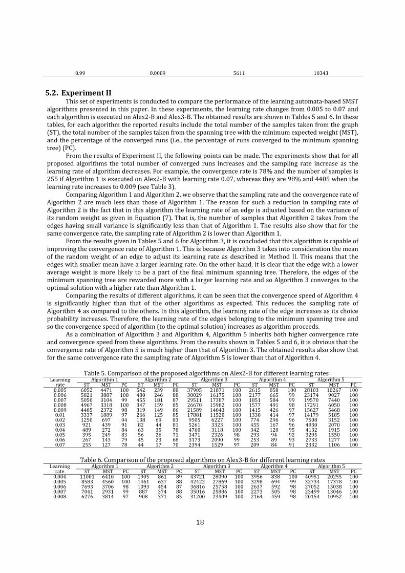
5.2. Experiment II This set of experiments is conducted to compare the performance of the learning automata‐based SMST
algorithms presented in this paper. In these experiments, the learning rate changes from 0.005 to 0.07 and each algorithm is executed on Alex2‐B and Alex3‐B. The obtained results are shown in Tables 5 and 6. In these tables, for each algorithm the reported results include the total number of the samples taken from the graph (ST), the total number of the samples taken from the spanning tree with the minimum expected weight (MST), and the percentage of the converged runs (i.e., the percentage of runs converged to the minimum spanning tree) (PC).
From the results of Experiment II, the following points can be made. The experiments show that for all proposed algorithms the total number of converged runs increases and the sampling rate increase as the learning rate of algorithm decreases. For example, the convergence rate is 78% and the number of samples is 255 if Algorithm 1 is executed on Alex2‐B with learning rate 0.07, whereas they are 98% and 4405 when the learning rate increases to 0.009 (see Table 3).
Comparing Algorithm 1 and Algorithm 2, we observe that the sampling rate and the convergence rate of Algorithm 2 are much less than those of Algorithm 1. The reason for such a reduction in sampling rate of Algorithm 2 is the fact that in this algorithm the learning rate of an edge is adjusted based on the variance of its random weight as given in Equation (7). That is, the number of samples that Algorithm 2 takes from the edges having small variance is significantly less than that of Algorithm 1. The results also show that for the same convergence rate, the sampling rate of Algorithm 2 is lower than Algorithm 1.
From the results given in Tables 5 and 6 for Algorithm 3, it is concluded that this algorithm is capable of improving the convergence rate of Algorithm 1. This is because Algorithm 3 takes into consideration the mean of the random weight of an edge to adjust its learning rate as described in Method II. This means that the edges with smaller mean have a larger learning rate. On the other hand, it is clear that the edge with a lower average weight is more likely to be a part of the final minimum spanning tree. Therefore, the edges of the minimum spanning tree are rewarded more with a larger learning rate and so Algorithm 3 converges to the optimal solution with a higher rate than Algorithm 1.
Comparing the results of different algorithms, it can be seen that the convergence speed of Algorithm 4 is significantly higher than that of the other algorithms as expected. This reduces the sampling rate of Algorithm 4 as compared to the others. In this algorithm, the learning rate of the edge increases as its choice probability increases. Therefore, the learning rate of the edges belonging to the minimum spanning tree and so the convergence speed of algorithm (to the optimal solution) increases as algorithm proceeds.
As a combination of Algorithm 3 and Algorithm 4, Algorithm 5 inherits both higher convergence rate and convergence speed from these algorithms. From the results shown in Tables 5 and 6, it is obvious that the convergence rate of Algorithm 5 is much higher than that of Algorithm 3. The obtained results also show that for the same convergence rate the sampling rate of Algorithm 5 is lower than that of Algorithm 4.
Table 5. Comparison of the proposed algorithms on Alex2‐B for different learning rates Algorithm 5Algorithm 4Algorithm 3Algorithm 2Algorithm 1 Learning
rate PCMSTST PC MSTSTPCMSTSTPCMST ST PC MST ST 1001026728103 100 8582615100218713790588239 542 100 4471 6052 0.005 100902723174 99 6652177100161753002988246 480 100 3887 5821 0.006 100744019570 99 5841851100173872951187181 455 99 3104 5050 0.007 100605017291 98 4911577100159822667085159 347 100 3318 4967 0.008 100546815627 97 4261415100140432158986149 319 98 2372 4405 0.009 100518514179 97 4141338100115201788185125 266 97 1889 3337 0.01 10031527508 96 296774100622795058369 138 94 697 1250 0.02 10020704930 96 167455100332352618144 82 91 439 921 0.03 10019154132 95 120342100311847607835 63 84 272 489 0.04 10015503295 92 9429398232634717126 56 83 249 395 0.05 10012772733 93 8925399209031736823 45 79 143 267 0.06 10011062332 91 8420997152923947017 44 78 127 255 0.07
Table 6. Comparison of the proposed algorithms on Alex3‐B for different learning rates Algorithm 5Algorithm 4 Algorithm 3Algorithm 2Algorithm 1 Learning
rate PCMSTST PC MSTSTPCMSTSTPCMST ST PC MST ST 1002025540951 100 83839561002809043721 89861 1905 100 6410 11001 0.004 1001737832734 99 6943298 1002786942422 88637 1461 100 4560 8583 0.005 1001503827052 98 59226371002575836816 87454 1093 98 3706 7693 0.006 1001304623499 98 50522731002588635016 88374 887 99 2931 7041 0.007 1001095220154 98 4592164100234093120085371 908 97 3814 6276 0.008
19
100998317951 96 41518231001598323663 82238 641 95 3176 5402 0.009 100901416191 97 3181615100135792066476237 511 94 2855 5258 0.01 10045568010 96 219865 100976913332 69137 310 90 1329 3203 0.02 10032985691 94 156598 10052937376 6279 157 86 548 1148 0.03 10025334293 92 11846910037985276 5981 141 80 422 857 0.04 10020113397 90 973699935254839 5652 107 72 261 532 0.05 10016772890 88 7930310022923259 5249 98 68 178 400 0.06 10014322461 88 7126198222230645541 65 67 140 278 0.07
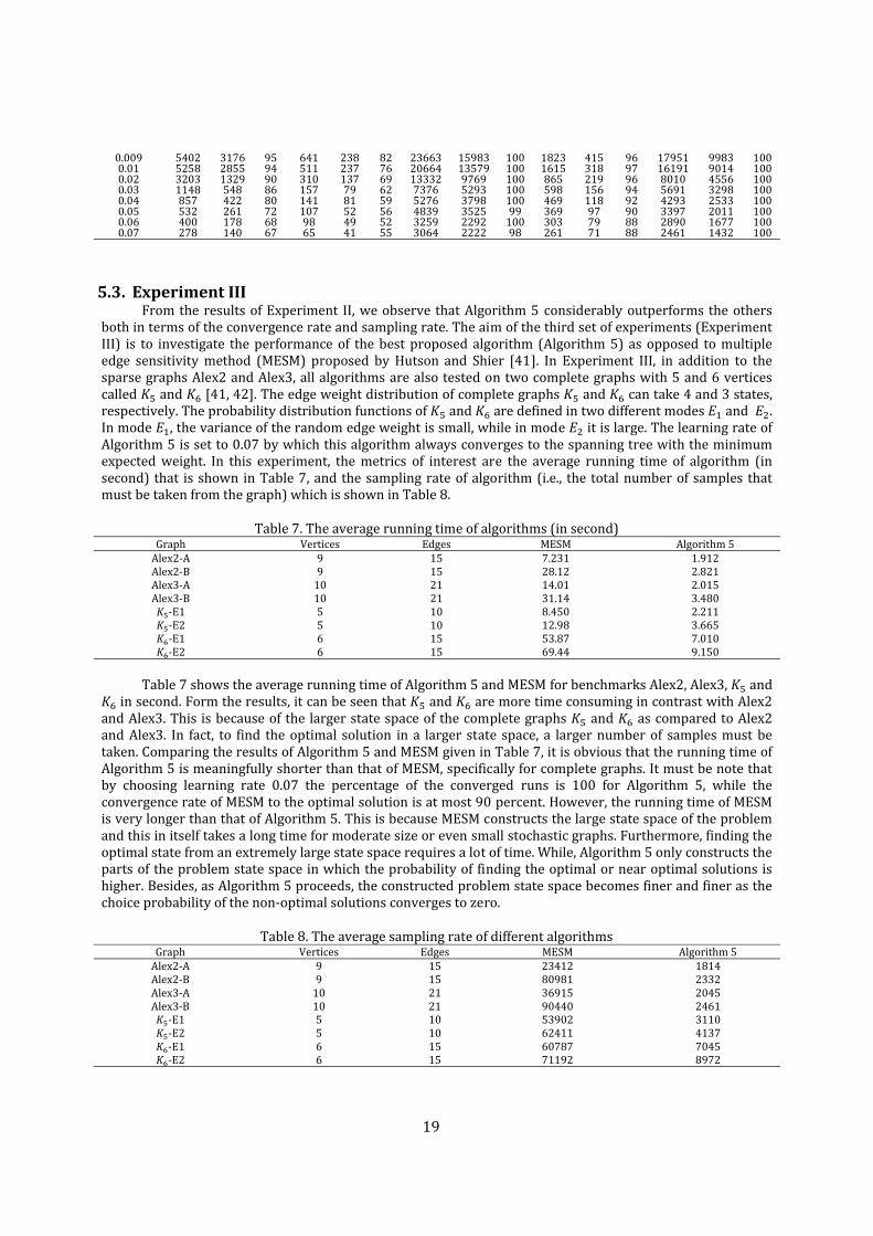
5.3. Experiment III From the results of Experiment II, we observe that Algorithm 5 considerably outperforms the others
both in terms of the convergence rate and sampling rate. The aim of the third set of experiments (Experiment III) is to investigate the performance of the best proposed algorithm (Algorithm 5) as opposed to multiple edge sensitivity method (MESM) proposed by Hutson and Shier [41]. In Experiment III, in addition to the sparse graphs Alex2 and Alex3, all algorithms are also tested on two complete graphs with 5 and 6 vertices called and [41, 42]. The edge weight distribution of complete graphs and can take 4 and 3 states, respectively. The probability distribution functions of and are defined in two different modes and . In mode , the variance of the random edge weight is small, while in mode it is large. The learning rate of Algorithm 5 is set to 0.07 by which this algorithm always converges to the spanning tree with the minimum expected weight. In this experiment, the metrics of interest are the average running time of algorithm (in second) that is shown in Table 7, and the sampling rate of algorithm (i.e., the total number of samples that must be taken from the graph) which is shown in Table 8.
Table 7. The average running time of algorithms (in second) Algorithm 5 MESM Edges Vertices Graph
1.912 7.231 159 Alex2‐A 2.821 28.12 15 9 Alex2‐B 2.015 14.01 21 10 Alex3‐A 3.480 31.14 2110 Alex3‐B 2.211 8.450 105 ‐E1 3.665 12.98 10 5 ‐E2 7.010 53.87 156 ‐E1 9.150 69.44 156 ‐E2
Table 7 shows the average running time of Algorithm 5 and MESM for benchmarks Alex2, Alex3, and
in second. Form the results, it can be seen that and are more time consuming in contrast with Alex2 and Alex3. This is because of the larger state space of the complete graphs and as compared to Alex2 and Alex3. In fact, to find the optimal solution in a larger state space, a larger number of samples must be taken. Comparing the results of Algorithm 5 and MESM given in Table 7, it is obvious that the running time of Algorithm 5 is meaningfully shorter than that of MESM, specifically for complete graphs. It must be note that by choosing learning rate 0.07 the percentage of the converged runs is 100 for Algorithm 5, while the convergence rate of MESM to the optimal solution is at most 90 percent. However, the running time of MESM is very longer than that of Algorithm 5. This is because MESM constructs the large state space of the problem and this in itself takes a long time for moderate size or even small stochastic graphs. Furthermore, finding the optimal state from an extremely large state space requires a lot of time. While, Algorithm 5 only constructs the parts of the problem state space in which the probability of finding the optimal or near optimal solutions is higher. Besides, as Algorithm 5 proceeds, the constructed problem state space becomes finer and finer as the choice probability of the non‐optimal solutions converges to zero.
Table 8. The average sampling rate of different algorithms Algorithm 5 MESM Edges Vertices Graph
1814 23412 159 Alex2‐A 2332 80981 159 Alex2‐B 2045 36915 21 10 Alex3‐A 2461 90440 21 10 Alex3‐B 3110 53902 105 ‐E1 4137 62411 10 5 ‐E2 7045 60787 15 6 ‐E1 8972 71192 156 ‐E2
20
Table 8 includes the results of the simulation experiments conducted to measure the sampling rate of
Algorithm 5 and MESM. From the obtained results, we observe that the sampling rate of Algorithm 5 is much less than that of MESM. This is because Algorithm 5 focuses on the sampling from the edges of the optimum spanning tree (avoids unnecessary samples) by excluding the non‐optimal edges (the edges that do not belong to the optimal spanning tree) from the sampling process at each stage. In MESM, sampling from the very huge state space of the stochastic problem results in a mush higher sampling rate compared to Algorithm 5. Briefly speaking, the higher convergence rate and lower sampling rate of Algorithm 5 confirm its superiority over MESM.
6. Conclusion In this paper, we first presented a learning automata‐based algorithm called Algorithm 1 for finding a
near optimal solution to the MST problem in stochastic graphs where the probability distribution function of the edge weight is unknown. The convergence of the proposed algorithm was theoretically proved. Convergence results confirmed that by a proper choice of the learning rate the probability of choosing the spanning tree with the minimum expected weight converges to one. Algorithm 1 was compared with the standard sampling method in terms of the sampling rate and the obtained results showed that this algorithm outperforms it. Then, to improve the convergence rate and convergence speed of Algorithm 1, we proposed four methods to adjust the learning rate of this algorithm. The algorithms in which the learning rate is determined by these four statistical methods were called as Algorithm 2 through Algorithm 5. Simulation experiments showed that Algorithm 5 performs better than the other algorithms in terms of the sampling and convergence rates and Algorithm 1 has the worst results. To show the performance of the best proposed SMST algorithm (Algorithm 5), we compared its results with those of the multiple edge sensitivity method (MESM) proposed by Hutson and Shier [41]. Experimental results confirmed the superiority of Algorithm 5 over MESM both in terms of the running time and sampling rate.
References [1] O. Boruvka, “O jistem Problemu Minimalnım (about a certain minimal problem),” Praca Moravske Prirodovedecke Spolecnosti, 1926, Vol. 3, pp. 37–58.
[2] J. B. Kruskal, “On the Shortest Spanning Sub Tree of a Graph and the Traveling Salesman Problem,” Proc. Amer. Math. Soc, 1956, Vol. pp. 748–750.
[3] R. C. Prim, “Shortest Connection Networks and Some Generalizations,” Bell. Syst. Tech. Journal, 1957, Vol. 36, pp. 1389–1401.
[4] H. Ishii, S. Shiode, T. Nishida and Y. Namasuya, "Stochastic Spanning Tree Problem," Discrete Applied Mathematics, 1981, Vol. 3, pp. 263‐273.
[5] H. lshii and T. Nishida, "Stochastic Bottleneck Spanning Tree Problem," Networks, 1983, Vol. 13, pp. 443‐449.
[6] I. B. Mohd, "Interval Elimination Method for Stochastic Spanning Tree Problem," Applied Mathematics and Computation, 1994, Vol. 66, pp. 325‐341.
[7] H. Ishii and T. Matsutomi, "Confidence Regional Method of Stochastic Spanning Tree Problem," Mathl. Comput. Modelling Vol. 22, No. 19‐12, 1995, pp. 77‐82.
[8] C. Alexopoulos and J. A. Jacobson, "State Space Partition Algorithms for Stochastic Systems with Applications to Minimum Spanning Trees," Networks, Vol. 35, No.2, 2000, pp. 118.138.
[9] K. Dhamdhere, R. Ravi and M. Singh, "On Two‐Stage Stochastic Minimum Spanning Trees," SpringerVerlag Berlin, 2005, pp. 321‐334.
21
[10] C. Swamy and D. B. Shmoys, " Algorithms Column: Approximation Algorithms for 2‐Stage Stochastic Optimization Problems," ACM SIGACT News, 2006, Vol. 37, No. 1, pp. 1‐16.
[11] M. A. L. Thathachar and B. R. Harita, "Learning Automata with Changing Number of Actions,” IEEE Transactions on Systems, Man, and Cybernetics, 1987, Vol. SMG17, pp. 1095‐1100.
[12] K. S. Narendra and K. S. Thathachar, "Learning Automata: An Introduction", New York, PrinticeHall, 1989.
[13] S. Lakshmivarahan and M. A. L. Thathachar, "Bounds on the Convergence Probabilities of Learning Automata," IEEE Transactions on Systems, Man, and Cybernetics, 1976, Vol. SMC‐6, pp. 756‐763.
[14] J. Zhou, E. Billard and S. Lakshmivarahan, " Learning in Multilevel Games with Incomplete Information‐Part II," IEEE Transactions on Syustem, Man, and, Cybernetics, 1999, Vol. 29, No.3, pp. 340‐349.
[15] M. A. L. Thathachar and P. S. Sastry, “A Hierarchical System of Learning Automata That Can Learn the Globally Optimal Path,” Information Science, 1997, Vol.42, pp.743‐766.
[16] M. A. L. Thathachar, V. V. Phansalkar, “Convergence of Teams and Hierarchies of Learning Automata in Connectionist Systems,” IEEE Transactions on Systems, Man and Cybernetics, 1995, Vol. 24, pp. 1459‐1469.
[17] S. Lakshmivarahan and K. S. Narendra, “Learning Algorithms for Two Person Zero‐sum Stochastic Games with Incomplete Information: A unified approach,” SIAM Journal of Control Optim., 1982, Vol. 20, pp. 541–552.
[18] K. S. Narenrdra and M. A. L. Thathachar, "On the Behavior of a Learning Automaton in a Changing Environment with Application to Telephone Traffic Routing," IEEE Transactions on Systems, Man, and, Cybernetics,1980, Vol. SMC‐l0, No. 5, pp. 262‐269.
[19] H. Beigy and M. R. Meybodi, “Utilizing Distributed Learning Automata to Solve Stochastic Shortest Path Problems,” International Journal of Uncertainty, Fuzziness and KnowledgeBased Systems, 2006, Vol.14, pp. 591‐615.
[20] R.G. Gallager, P.A. Humblet and P.M. Spira, “A Distributed Algorithm for Minimum Weight Spanning Trees,” ACM Trans. on Program. Lang. & Systems, 1983, Vol. 5, pp. 66‐77.
[21] F. Chin and H.F. Ting, “An Almost Linear Time and O(n log n + e) Messages Distributed Algorithm for Minimum‐Weight Spanning Trees,” in Proceedings of the 26th IEEE Symposium on Foundations of Computer Science (FOCS), 1985, pp. 257‐ 266.
[22] E. Gafni, “Improvements in the Time Complexity of Two Message‐Optimal Election Algorithms,” in Proceedings s of the 4th Symposium on Principles of Distributed Computing (PODC), 1985, pp. 175‐185.
[23] B. Awerbuch, “Optimal Distributed Algorithms for Minimum Weight Spanning Tree, Counting, Leader Election, and Related Problems,” in Proceedings of the 19th ACM Symposium on Theory of Computing (STOC), 1987, pp 230‐240.
[24] J. Garay, S. Kutten, and D. Peleg, “A Sublinear Time Distributed Algorithm for Minimum‐Weight Spanning Trees,” SIAM Journal of Computing, 1998, Vol. 27, pp. 302‐316.
[25] M. Elkin, “Unconditional Lower Bounds on the Time‐Approximation Tradeoffs for the Distributed Minimum Spanning Tree Problem,” in Proceedings of the ACM Symposium on Theory of Computing (STOC), 2004, pp. 331‐340.
[26] M. Elkin, “An Overview of Distributed Approximation,” ACM SIGACT News Distributed Computing Column, 2004, Vol. 35 No. 4, pp. 40‐57.
22
[27] M. Khan and G. Pandurangan, “A Fast Distributed Approximation Algorithm for Minimum Spanning Trees,” in Proceedings of the 20th International Symposium on Distributed Computing (DISC), September 2006.
[28] F. B. ALT, “Bonferroni Inequalities and Intervals,” in Encyclopedia of Statistical Sciences, 1982, Vol. 1, pp. 294–301.
[29] C. E. Bonferroni, "Teoria Statistica Delle Classi e Calcolo Delle Probabilit`a," Pubblicazioni del R Istituto Superiore di Scienze Economiche e Commerciali di Firenze, 1936, Vol. 8, pp. 3–62.
[30] S. Holm, "A Simple Sequentially Rejective Multiple Test Procedure," Scandinavian Journal of Statistics, 1979, Vol. 6, pp. 65–70.
[31] S. Marchand‐Maillet, Y. M. Sharaiha, “A Minimum Spanning Tree Approach to Line Image Analysis,” in Proceedings of 13th International Conference on Pattern Recognition (ICPR'96), 1996, pp. 225.
[32] J. Li, S. Yang, X. Wang, X. Xue, and B. Li, “Tree‐structured Data Regeneration with Network Coding in Distributed Storage Systems,” in Proceedings of International Conference on Image Processing, Charleston, USA, 2009, pp. 481–484.
[33] J. C. Gower, and G. J. S. Ross, “Minimum Spanning Trees and Single Linkage Cluster Analysis,” Journal of the Royal Statistical Society (Applied Statistics), 1969, Vol. 18, No. 1, pp. 54‐64.
[34] Z. Barzily, Z. Volkovich, B. Akteke‐Öztürk, G. W. Weber, “On a Minimal Spanning Tree Approach in the Cluster Validation Problem,” Informatica, 2009, Vol. 20, No. 2, pp. 187‐202.
[35] R. E. Osteen, and P. P. Lin, “Picture Skeletons Based on Eccentricities of Points of Minimum Spanning Trees,” SIAM Journal on Computing, 1974, Vol. 3, pp. 23‐40.
[36] T. C. Chiang, C. H. Liu, and Y.M. Huang, “A Near‐Optimal Multicast Scheme for Mobile Ad hoc Networks Using a Hybrid Genetic Algorithm,” Expert Systems with Applications, 2007, Vol. 33 pp. 734–742.
[37] G. Rodolakis, A. Laouiti, P. Jacquet, and A. M. Naimi, “Multicast Overlay Spanning Trees in Ad hoc Networks: Capacity bounds protocol design and performance evaluation,” Computer Communications, 2008, Vol. 31, pp. 1400‐1412.
[38] H. Katagiri, E. B. Mermri, M. Sakawa and K. Kato, “A Study on Fuzzy Random Minimum Spanning Tree Problems through Possibilistic Programming and the Expectation Optimization Model,” in Proceedings of the 47th IEEE International Midwest Symposium on Circuits and Systems, 2004.
[39] H. Fangguo, and Q. Huan, “A Model and Algorithm for Minimum Spanning Tree Problems in Uncertain Networks,” in Proceedings of the 3rd International Conference on Innovative Computing Information and Control (ICICIC'08), 2008.
[40] T. A. Almeida, A. Yamakami, and M. T. Takahashi, “An Evolutionary Approach to Solve Minimum Spanning Tree Problem with Fuzzy Parameters,” in Proceedings of the International Conference on Computational Intelligence for Modelling, Control and Automation, 2005.
[41] K. R. Hutson, and D. R. Shier, “Minimum Spanning Trees in Networks with varying Edge Weights,” Annals of Operations Research, Vol. 146, pp. 3–18, 2006.
[42] K. R. Hutson, and D. R. Shier, “Bounding Distributions for the Weight of a Minimum Spanning Tree in Stochastic Networks,” Operations Research, 2005, Vol. 53, No. 5, pp. 879‐886.
23
[43] J. Akbari Torkestani, and M. R. Meybodi, "A Learning Automata‐based Cognitive Radio for Clustered Wireless Ad‐Hoc Networks", Journal of Network and Systems Management, 2011, Vol. 19, No. 2, pp. 278‐297.
[44] J. Akbari Torkestani, and M. R. Meybodi, “A Learning automata‐based Heuristic Algorithm for Solving the Minimum Spanning Tree Problem in Stochastic Graphs,” Journal of Supercomputing, Springer Publishing Company, 2010, in press.
[45] J. Akbari Torkestani, and M. R. Meybodi, “Learning Automata‐Based Algorithms for Finding Minimum Weakly Connected Dominating Set in Stochastic Graphs,” International Journal of Uncertainty, Fuzziness and Knowledge‐based Systems, 2010, Vol. 18, No. 6, pp. 721‐758.
[46] J. Akbari Torkestani, and M. R. Meybodi, “Mobility‐based Multicast Routing Algorithm in Wireless Mobile Ad Hoc Networks: A Learning Automata Approach,” Journal of Computer Communications, 2010, Vol. 33, pp. 721‐735.
[47] J. Akbari Torkestani, and M. R. Meybodi, “A New Vertex Coloring Algorithm Based on Variable Action‐Set Learning Automata,” Journal of Computing and Informatics, 2010, Vol. 29, No. 3, pp. 1001‐1020.
[48] J. Akbari Torkestani, and M. R. Meybodi, “Weighted Steiner Connected Dominating Set and its Application to Multicast Routing in Wireless MANETs,” Wireless Personal Communications, Springer Publishing Company, 2010, in press.
[49] J. Akbari Torkestani, and M. R. Meybodi, “An Efficient Cluster‐based CDMA/TDMA Scheme for Wireless Mobile AD‐Hoc Networks: A Learning Automata Approach,” Journal of Network and Computer applications, 2010, Vol. 33, pp. 477‐490.
[50] J. Akbari Torkestani, and M. R. Meybodi, “Clustering the Wireless Ad‐Hoc Networks: A Distributed Learning Automata Approach,” Journal of Parallel and Distributed Computing, 2010, Vol. 70, pp. 394‐405.
[51] J. Akbari Torkestani, and M. R. Meybodi, “An Intelligent Backbone Formation Algorithm in Wireless Ad Hoc Networks based on Distributed Learning Automata,” Journal of Computer Networks, 2010, Vol. 54, pp. 826‐843.
[52] J. Akbari Torkestani, and M. R. Meybodi, “A Mobility‐based Cluster Formation Algorithm for Wireless Mobile Ad Hoc Networks,” Journal of Cluster Computing, Springer Publishing Company, 2011, in press.
[53] J. Akbari Torkestani, and M. R. Meybodi, “A Cellular Learning Automata‐based Algorithm for Solving the Vertex Coloring Problem,” Journal of Expert Systems with Applications, 2011, in press.