Dynamic modelling of flexibly supported gears using iterative

convergence of tooth mesh stiffness

Song Xue, Ian Howard*

Department of Mechanical Engineering, Curtin University, Bentley, Western Australia, Australia Department of Mechanical Engineering, Curtin University of Technology, GPO Box U1987, Perth,

WA 6845, Australia

* Corresponding author. Phone: (+61) 89266 7047.

E-mail: i.howard@curtin.edu.au

Abstract: This paper presents a new gear dynamic model for flexibly supported gear sets aiming to

improve the accuracy of gear fault diagnostic methods. In the model, the operating gear centre distance, which

can affect the gear design parameters, like the gear mesh stiffness, has been selected as the iteration criteria

because it will significantly deviate from its nominal value for a flexible supported gearset when it is operating.

The FEA method was developed for calculation of the gear mesh stiffnesses with varying gear centre distance,

which can then be incorporated by iteration into the gear dynamic model. The dynamic simulation results from

previous models that neglect the operating gear centre distance change and those from the new model that

incorporate the operating gear centre distance change were obtained by numerical integration of the differential

equations of motion using the Newmark method. Some common diagnostic tools were utilized to investigate the

difference and comparison of the fault diagnostic results between the two models. The results of this paper

indicate that the major difference between the two diagnostic results for the cracked tooth exists in the extended

duration of the crack event and in changes to the phase modulation of the coherent time synchronous averaged

signal even though other notable differences from other diagnostic results can also be observed.

Keyword: Gear dynamics, Mesh stiffness, Tooth fault, Gear fault diagnostics, phase modulation

1 Introduction

Gears are considered to be one of the most widely used mechanical components in various applications,

including automotive, aerospace and mining. However, noise and vibration, reliability and early detection of

gear damage remain major concerns in their applications. As a result, gearbox vibration condition monitoring is

an important aspect of engineering maintenance.

Dynamic modelling of gear vibration can be used to further the understanding of the vibration generation

mechanisms in gear transmissions as well as the dynamic behaviour of the transmission in the presence of

various types of gear faults. A comprehensive review of gear dynamic models can be found in [1]. Among the

various models, the coupled torsional and transverse model is one of the common modelling approaches that

have been used recently. The advantage of this model is that it includes the flexibility of the shaft and bearings

as well as the tooth mesh deformation and therefore, the dynamic response from this type of model is more

realistic and closer to the measured vibration data [1-6]. Mathematical gear simulation, where both torsional and

lateral vibrations have been considered, has been used as an aid to gearbox diagnostics [2]. It suggests that a

one-stage gearbox model which consists of a motor, couplings, and a driven machine is the best approach for

investigation of the gear dynamic behaviour. Based on the model developed by Du [3], Howard et al. developed

a 16-degree-of-freedom gear dynamic model which included the effect of friction and the effect of a tooth crack

[4]. Some diagnostic techniques were used to deal with the resultant vibration signal and it showed that the

result obtained from the simulation was very similar to that observed from a helicopter gearbox, but in most

cases, friction gave a negligible change in the resulting diagnostic value. Later on, a 26-degree-of-freedom gear

dynamic model which included three shafts and two pairs of gears in mesh was developed for the purpose of

comparing localised tooth spalling and damage [5]. The effect of spalling and tooth breakage on the gear mesh

stiffness was analytical formulated and then the resultant gear mesh stiffness curves was incorporated into a

one-stage spur gear model where the flexibility of the shaft and bearing was considered [6].

One of the major assumptions in these models mentioned above is that gear pairs are intended to mesh on

standard centre distance and its contribution to the change of the gear design parameters, such as pressure angle,

contact ratio and even the gear mesh stiffness, is limited. In fact, the actual operating gear centre distance is

influenced by the combined effects of manufacturing tolerances, bearing backlash and deflections in the support

structure [7]. Especially for a flexible supported gear system, the change of the operating gear centre distance

from its nominal value cannot be neglected and therefore, the dynamic performance induced by the change of

the gear centre distance is expected to be different.

However, few studies have been found that were focused on the influence of gear centre distance on the gear

dynamic performance. Hsiang His Lin presented an analytical study on using hob offset to balance the dynamic

tooth strength of spur gears operating at a centre distance greater than the standard value [8]. A new dynamic

model considering the time-varying gear centre distance was proposed in [9]. They found that the bearing

stiffness had a significant effect upon the gear vibration. Later, they extended the time-varying factor to

planetary gear systems, finding that the dynamic response of planetary gears with time-varying pressure angles

and contact ratios had more frequency components than the dynamic responses with constant pressure angles

and contact ratios [10]. Despite these publications, there remains a paucity of research on the effect of the gear

centre distance variation on the gear dynamic performance, and the gear centre distance variation on the

resulting gear fault diagnosis methods.

In this paper, a new gear dynamic model is proposed that considers the gear centre distance variation, which has

been selected as the iteration criteria to ascertain the accuracy of the dynamic response. Based on the dynamic

response, some common diagnostic techniques are used to examine the gear system vibration behaviour results

compared with the results from the model without considering the gear centre distance variation. The first

section of this paper derives the differential equations used for the gear system. The finite element analysis

(FEA) method was then used to analysis the gear mesh stiffness with different gear centre distance changes. The

effect of a 5 mm root crack on the gear mesh stiffness curve has also been modelled with different gear centre

distances. As the change of the gear mesh stiffness largely relies on the variation of the gear centre distance, a

subsequent iteration strategy was developed by comparing the gear centre distance at two nearby time steps.

This was then used in the gear dynamic model to ensure the gear dynamic solution convergence at each time

step as outlined in the third section. The fourth section compares the findings of the diagnostic results, which

have been examined by coherent time synchronous averaging, followed by root mean squared (RMS) spectrum

analysis, residual signal, Pseudo Wigner-Ville distribution (PWVD), narrow band envelope, amplitude

modulation, phase modulation and analytic signal plots.

2 Modelling of Spur Gears considering the gear centre variation

2.1 Influence of gear centre distance variation

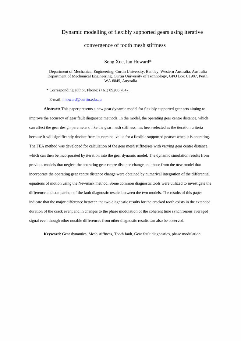
The centre distance of a gear pair in mesh is determined by the pinion and gear geometry, as shown in Fig. 1. In

the reference coordinate, the designed position for the pinion centre is Op and the designed position for the gear

centre is Og. On the application of input load displacements will occur in the vertical direction while there will

be no displacement in the horizontal direction because the friction force is neglected. The resulting pinion centre

will change from position Op to position Op’ and the gear centre will change from position Og to position Og’. In

the reference coordinate, the operating position for the pinion centre Op’ is,

𝑑𝑑𝑝𝑝����⃑ = (0)�⃑�𝑥 + �𝑦𝑦𝑝𝑝��⃑�𝑦, (1)

and the operating position for the gear centre Og’ is,

𝑑𝑑𝑔𝑔����⃑ = �𝑟𝑟𝑝𝑝 + 𝑟𝑟𝑔𝑔��⃑�𝑥 + ��𝑟𝑟𝑝𝑝 + 𝑟𝑟𝑔𝑔� tan𝛼𝛼 + 𝑦𝑦𝑔𝑔� �⃑�𝑦, (2)

where rp is the base radius of the pinion and rg is the base radius of the gear and α is the designed pressure angle.

Fig. 1 Spur gear centre distance variation

From Fig.1, it can be found that the designed gear centre distance d is,

𝑑𝑑 =𝑟𝑟𝑃𝑃 + 𝑟𝑟𝑔𝑔cos𝛼𝛼

, (3)

The operating gear centre distance 𝑑𝑑′ is,

𝑑𝑑′ = ���𝑟𝑟𝑝𝑝 + 𝑟𝑟𝑔𝑔��2 + [�𝑟𝑟𝑝𝑝 + 𝑟𝑟𝑔𝑔� tan𝛼𝛼 + 𝑦𝑦𝑔𝑔 − 𝑦𝑦𝑝𝑝]2. (4)

The designed pressure angle α is,

𝛼𝛼 = cos−1𝑟𝑟𝑃𝑃 + 𝑟𝑟𝑔𝑔𝑑𝑑

, (5)

while the operating gear pressure angle 𝛼𝛼′will become,

𝛼𝛼′ = cos−1𝑟𝑟𝑃𝑃 + 𝑟𝑟𝑔𝑔𝑑𝑑′

, (6)

The designed gear contact ratio mp is,

𝑚𝑚𝑝𝑝 =�𝑟𝑟𝑎𝑎𝑝𝑝2 − 𝑟𝑟𝑝𝑝2 + �𝑟𝑟𝑎𝑎𝑔𝑔2 − 𝑟𝑟𝑔𝑔2 − 𝑑𝑑 sin𝛼𝛼

𝜋𝜋 ∙ 𝑚𝑚 ∙ cos𝛼𝛼, (7)

where rap is the addendum radius of the pinion and rag is the addendum radius of the gear and m is the gear module. The operating gear contact ratio 𝑚𝑚𝑝𝑝

′ will become,

𝑚𝑚𝑝𝑝′ =

�𝑟𝑟𝑎𝑎𝑝𝑝2 − 𝑟𝑟𝑝𝑝2 + �𝑟𝑟𝑎𝑎𝑔𝑔2 − 𝑟𝑟𝑔𝑔2 − 𝑑𝑑′ sin𝛼𝛼′

𝜋𝜋 ∙ 𝑚𝑚 ∙ cos𝛼𝛼′, (8)

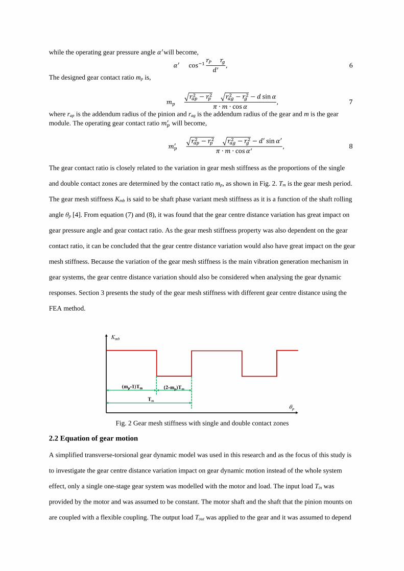
The gear contact ratio is closely related to the variation in gear mesh stiffness as the proportions of the single

and double contact zones are determined by the contact ratio mp, as shown in Fig. 2. Tm is the gear mesh period.

The gear mesh stiffness Kmb is said to be shaft phase variant mesh stiffness as it is a function of the shaft rolling

angle θp [4]. From equation (7) and (8), it was found that the gear centre distance variation has great impact on

gear pressure angle and gear contact ratio. As the gear mesh stiffness property was also dependent on the gear

contact ratio, it can be concluded that the gear centre distance variation would also have great impact on the gear

mesh stiffness. Because the variation of the gear mesh stiffness is the main vibration generation mechanism in

gear systems, the gear centre distance variation should also be considered when analysing the gear dynamic

responses. Section 3 presents the study of the gear mesh stiffness with different gear centre distance using the

FEA method.

Fig. 2 Gear mesh stiffness with single and double contact zones

2.2 Equation of gear motion

A simplified transverse-torsional gear dynamic model was used in this research and as the focus of this study is

to investigate the gear centre distance variation impact on gear dynamic motion instead of the whole system

effect, only a single one-stage gear system was modelled with the motor and load. The input load Tin was

provided by the motor and was assumed to be constant. The motor shaft and the shaft that the pinion mounts on

are coupled with a flexible coupling. The output load Tout was applied to the gear and it was assumed to depend

on the gear angular velocity. A flexible coupling was also attached between the output load and gear shafts. A

linear bearing arrangement was used to connect the gear centre, the ground and the bearing and includes the

radial stiffness kij (i=x, y; j=p,g), radial damping qij (i=x, y; j=p,g) and torsional damping qstj (i=x, y; j=p,g).

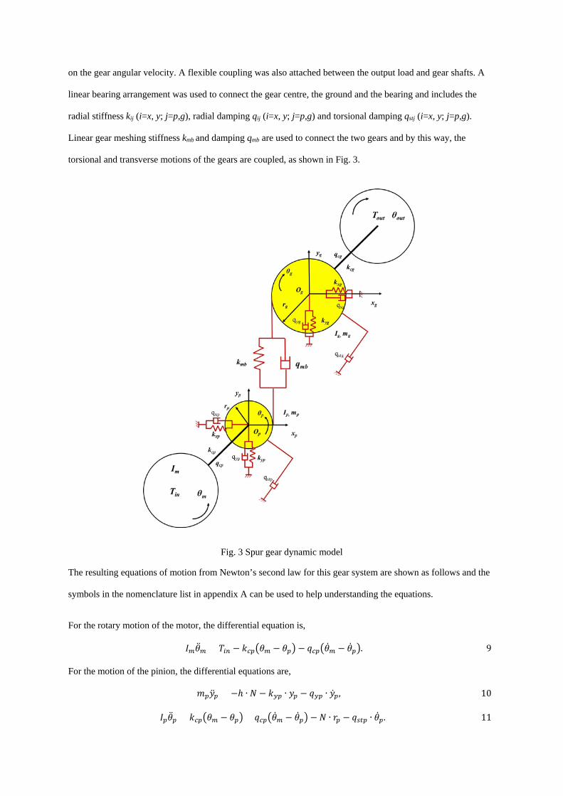
Linear gear meshing stiffness kmb and damping qmb are used to connect the two gears and by this way, the

torsional and transverse motions of the gears are coupled, as shown in Fig. 3.

Fig. 3 Spur gear dynamic model

The resulting equations of motion from Newton’s second law for this gear system are shown as follows and the

symbols in the nomenclature list in appendix A can be used to help understanding the equations.

For the rotary motion of the motor, the differential equation is,

𝐼𝐼𝑚𝑚�̈�𝜃𝑚𝑚 = 𝑇𝑇𝑖𝑖𝑖𝑖 − 𝑘𝑘𝑐𝑐𝑝𝑝�𝜃𝜃𝑚𝑚 − 𝜃𝜃𝑝𝑝� − 𝑞𝑞𝑐𝑐𝑝𝑝��̇�𝜃𝑚𝑚 − �̇�𝜃𝑝𝑝�. (9)

For the motion of the pinion, the differential equations are,

𝑚𝑚𝑝𝑝�̈�𝑦𝑝𝑝 = −ℎ ∙ 𝑁𝑁 − 𝑘𝑘𝑦𝑦𝑝𝑝 ∙ 𝑦𝑦𝑝𝑝 − 𝑞𝑞𝑦𝑦𝑝𝑝 ∙ �̇�𝑦𝑝𝑝, (10)

𝐼𝐼𝑝𝑝�̈�𝜃𝑝𝑝 = 𝑘𝑘𝑐𝑐𝑝𝑝�𝜃𝜃𝑚𝑚 − 𝜃𝜃𝑝𝑝� + 𝑞𝑞𝑐𝑐𝑝𝑝��̇�𝜃𝑚𝑚 − �̇�𝜃𝑝𝑝� − 𝑁𝑁 ∙ 𝑟𝑟𝑝𝑝 − 𝑞𝑞𝑠𝑠𝑠𝑠𝑝𝑝 ∙ �̇�𝜃𝑝𝑝. (11)

For the motion of the gear, the differential equations are,

𝑚𝑚𝑔𝑔�̈�𝑦𝑔𝑔 = ℎ ∙ 𝑁𝑁 − 𝑘𝑘𝑦𝑦𝑔𝑔 ∙ 𝑦𝑦𝑔𝑔 − 𝑞𝑞𝑦𝑦𝑔𝑔 ∙ �̇�𝑦𝑔𝑔, (12)

𝐼𝐼𝑔𝑔�̈�𝜃𝑔𝑔 = ℎ ∙ 𝑁𝑁 ∙ 𝑟𝑟𝑔𝑔 − 𝑘𝑘𝑐𝑐𝑔𝑔�𝜃𝜃𝑔𝑔 − 𝜃𝜃𝑜𝑜𝑜𝑜𝑠𝑠� − 𝑞𝑞𝑐𝑐𝑔𝑔��̇�𝜃𝑔𝑔 − �̇�𝜃𝑜𝑜𝑜𝑜𝑠𝑠� − 𝑞𝑞𝑠𝑠𝑠𝑠𝑝𝑝 ∙ �̇�𝜃𝑔𝑔, (13)

where N is the normal contact force between pinion and gear and is given by,

𝑁𝑁 = 𝑘𝑘𝑚𝑚𝑚𝑚 ∙ �𝑦𝑦𝑝𝑝 + 𝑟𝑟𝑝𝑝 ∙ 𝜃𝜃𝑝𝑝 − 𝑦𝑦𝑔𝑔 − 𝑟𝑟𝑔𝑔 ∙ 𝜃𝜃𝑔𝑔� + 𝑞𝑞𝑚𝑚𝑚𝑚 ∙ ��̇�𝑦𝑝𝑝 + 𝑟𝑟𝑝𝑝 ∙ �̇�𝜃𝑝𝑝 − �̇�𝑦𝑔𝑔 − 𝑟𝑟𝑔𝑔 ∙ �̇�𝜃𝑔𝑔�. (14)

h is a unit step function that can be used to represent the tooth separation phenomenon,

ℎ = �1,𝑝𝑝 ≥ 0 0,𝑝𝑝 < 0 ,

where p represents the relative gear mesh displacement defined as,

𝑝𝑝 = 𝑦𝑦𝑝𝑝 + 𝑟𝑟𝑝𝑝 ∙ 𝜃𝜃𝑝𝑝 − 𝑦𝑦𝑔𝑔 − 𝑟𝑟𝑔𝑔 ∙ 𝜃𝜃𝑔𝑔. (15)

In this way, if p is at a position where the relative gear mesh displacement has a negative value, the teeth will

lose contact and the resulting spring force will be equal to zero.

For the rotary motion of the load, the differential equation of motion becomes,

𝐼𝐼𝑜𝑜𝑜𝑜𝑠𝑠�̈�𝜃𝑜𝑜𝑜𝑜𝑠𝑠 = −𝑇𝑇𝑜𝑜𝑜𝑜𝑠𝑠 + 𝑘𝑘𝑐𝑐𝑔𝑔�𝜃𝜃𝑔𝑔 − 𝜃𝜃𝑜𝑜𝑜𝑜𝑠𝑠�+ 𝑞𝑞𝑐𝑐𝑔𝑔��̇�𝜃𝑔𝑔 − �̇�𝜃𝑜𝑜𝑜𝑜𝑠𝑠�. (16)

The derived differential gear equations of motion can be represented in matrix-vector form. This matrix-vector

form is useful in computing dynamic responses when applying numerical time integration algorithms. The

matrix-vector form of the nonlinear equations can be written as,

𝑀𝑀�̈�𝑥 + 𝐶𝐶�̇�𝑥 + 𝐾𝐾𝑥𝑥 = 𝐹𝐹, (17)

where �̈�𝑥 is the 1×6 acceleration vector, �̇�𝑥 is the 1×6 speed vector, x is the 1×6 displacement vector, M is

the 6×6 mass matrix, K is the 6×6 stiffness matrix, C is the 6×6 damping matrix and F is the 1×6 external

loading force. The details of these matrixes can be found in appendix B.

3 Effect of gear centre distance variation on gear mesh stiffness using FEA methods

As analysed in section 2.1, the gear mesh stiffness will be affected by the gear centre distance in both magnitude

and phase. In this section, FEA models were developed to study the effect of gear centre distance variation on

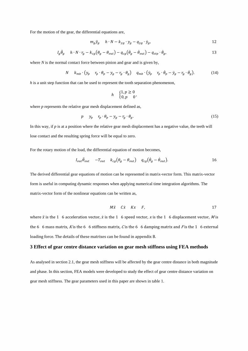
gear mesh stiffness. The gear parameters used in this paper are shown in table 1.

Table 1 Gear parameters

Number of teeth, pinion, Zp 23 Number of teeth, gear, Zg 23

Module, mn 6 mm Designed pressure angle, α 20º

Base radius, pinion, rp 129.7 mm Base radius, gear, rg 129.7 mm

Designed gear centre distance, d 138 mm Designed gear contact ratio, ctr 1.59

Young’s modulus, E 69 GPa Mass, pinion, mp 0.7 kg Mass, gear, mg 0.7 kg

Moment of inertia, Ip 0.0025 kgm2 Moment of inertia, Ig 0.0025 kgm2

Pinion bearing stiffness, N/m 1×106 Gear bearing stiffness, N/m 1×106

The detailed method of calculating gear torsional mesh stiffness can be found in [11]. Using the strategy

mentioned in [11], one FEA spur gear model with one pinion and one gear can be obtained. The whole gear

model can then be moved intentionally in the vertical direction with a distance increment of ∆d, as shown in Fig.

4. This results in a new gear centre distance d+∆d, where distance increment ∆d will also introduce a backlash

ΔB=2·Δd·tanα between the pinion involute profile and the gear involute profile. As a result, an imposed

displacement of Δd·tanα/rpp can be introduced to the pinion gear hub to eliminate the backlash ΔB. After

rotation, the adaptive re-mesh method can be used at each contact position. The weak spring connected with the

pinion hub node method is also needed followed by the element birth & death command to disable the weak

spring after the pinion moves to be just in contact with the gear profile.

Fig. 4 FEA gear model with distance increment

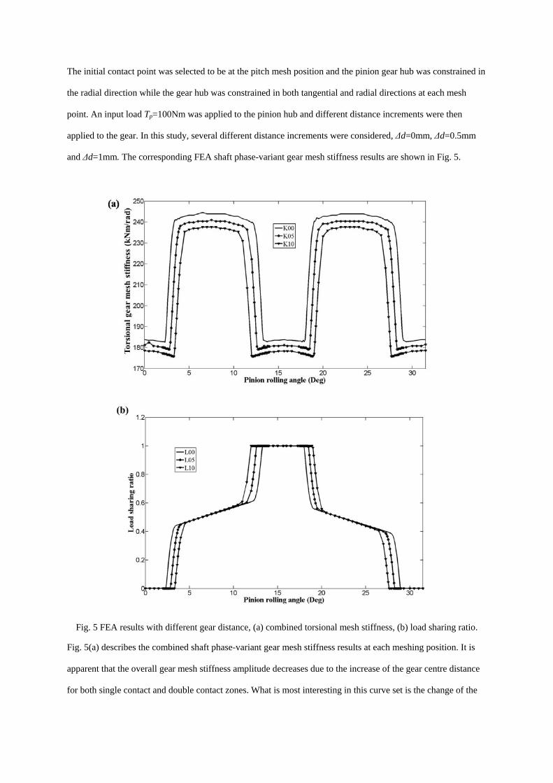
The initial contact point was selected to be at the pitch mesh position and the pinion gear hub was constrained in

the radial direction while the gear hub was constrained in both tangential and radial directions at each mesh

point. An input load Tp=100Nm was applied to the pinion hub and different distance increments were then

applied to the gear. In this study, several different distance increments were considered, Δd=0mm, Δd=0.5mm

and Δd=1mm. The corresponding FEA shaft phase-variant gear mesh stiffness results are shown in Fig. 5.

Fig. 5 FEA results with different gear distance, (a) combined torsional mesh stiffness, (b) load sharing ratio.

Fig. 5(a) describes the combined shaft phase-variant gear mesh stiffness results at each meshing position. It is

apparent that the overall gear mesh stiffness amplitude decreases due to the increase of the gear centre distance

for both single contact and double contact zones. What is most interesting in this curve set is the change of the

proportions of the single and double contact zones, which will result in a phase lag when the adjacent gear tooth

comes into mesh. This mesh lag can also be seen in the load sharing ratio plot, in Fig 5(b). With the increase of

the gear centre distance, the length of the single contact zone, whose length is (2-mp)Tm, increases while the

length of the double contact zone, whose length is (mp-1)Tm, decreases accordingly. Traditionally, only the K00

curve will be interpolated into the gear dynamic equation when the gear dynamic response was studied, no

matter what the gear centre distance variation was. In other words, the gear mesh stiffness was assumed to be

only the function of the pinion rolling angle. However, if the gear centre distance increment varies from 0mm to

1mm during the operation, the mesh stiffness will have to vary between K00 and K10 accordingly, which will

result in a dramatically different dynamic response.

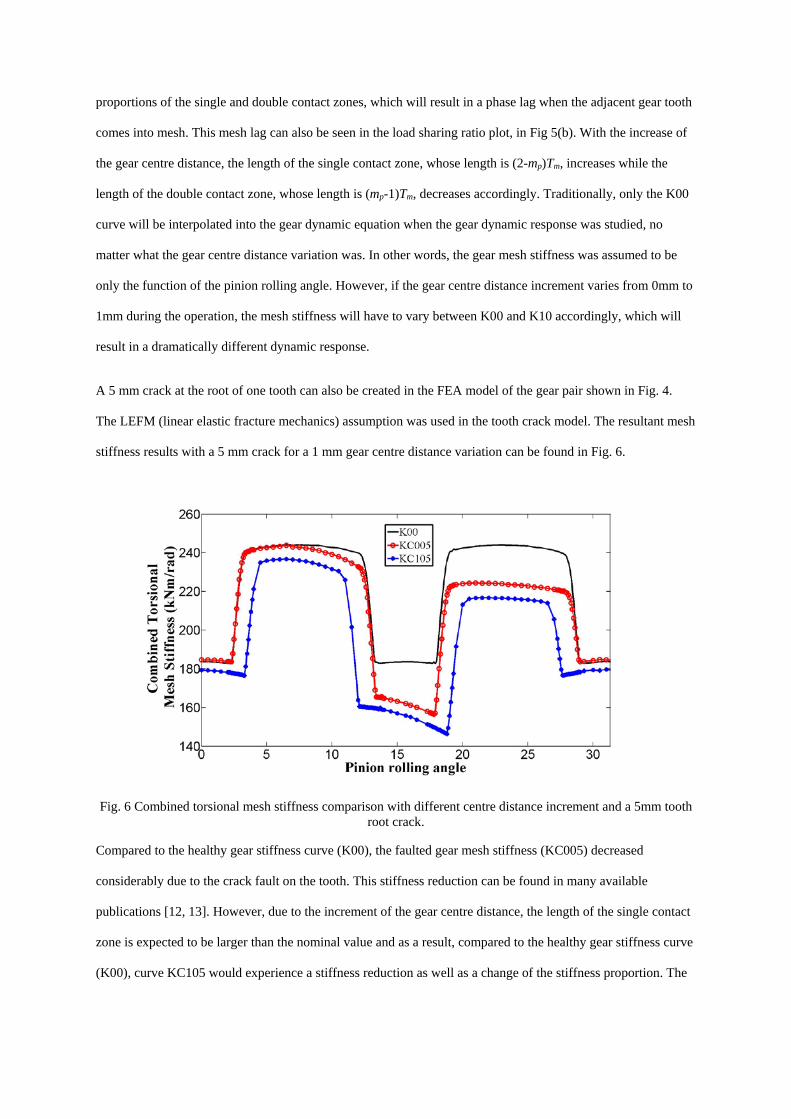
A 5 mm crack at the root of one tooth can also be created in the FEA model of the gear pair shown in Fig. 4.

The LEFM (linear elastic fracture mechanics) assumption was used in the tooth crack model. The resultant mesh

stiffness results with a 5 mm crack for a 1 mm gear centre distance variation can be found in Fig. 6.

Fig. 6 Combined torsional mesh stiffness comparison with different centre distance increment and a 5mm tooth root crack.

Compared to the healthy gear stiffness curve (K00), the faulted gear mesh stiffness (KC005) decreased

considerably due to the crack fault on the tooth. This stiffness reduction can be found in many available

publications [12, 13]. However, due to the increment of the gear centre distance, the length of the single contact

zone is expected to be larger than the nominal value and as a result, compared to the healthy gear stiffness curve

(K00), curve KC105 would experience a stiffness reduction as well as a change of the stiffness proportion. The

dynamic gear system response caused by curve KC105 would therefore be expected to be different from the

dynamic response caused by curve KC005.

4 Numerical simulation and result discussion

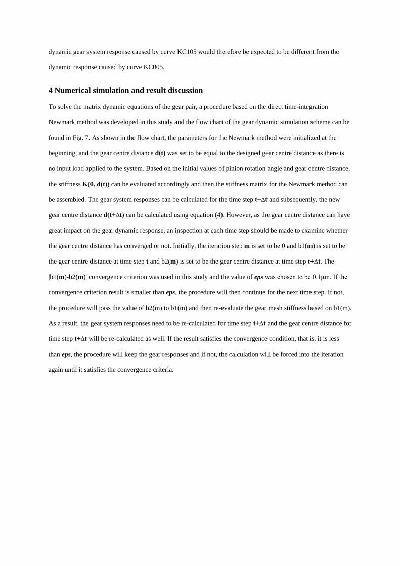
To solve the matrix dynamic equations of the gear pair, a procedure based on the direct time-integration

Newmark method was developed in this study and the flow chart of the gear dynamic simulation scheme can be

found in Fig. 7. As shown in the flow chart, the parameters for the Newmark method were initialized at the

beginning, and the gear centre distance d(t) was set to be equal to the designed gear centre distance as there is

no input load applied to the system. Based on the initial values of pinion rotation angle and gear centre distance,

the stiffness K(θ, d(t)) can be evaluated accordingly and then the stiffness matrix for the Newmark method can

be assembled. The gear system responses can be calculated for the time step t+∆t and subsequently, the new

gear centre distance d(t+∆t) can be calculated using equation (4). However, as the gear centre distance can have

great impact on the gear dynamic response, an inspection at each time step should be made to examine whether

the gear centre distance has converged or not. Initially, the iteration step m is set to be 0 and b1(m) is set to be

the gear centre distance at time step t and b2(m) is set to be the gear centre distance at time step t+∆t. The

|b1(m)-b2(m)| convergence criterion was used in this study and the value of eps was chosen to be 0.1μm. If the

convergence criterion result is smaller than eps, the procedure will then continue for the next time step. If not,

the procedure will pass the value of b2(m) to b1(m) and then re-evaluate the gear mesh stiffness based on b1(m).

As a result, the gear system responses need to be re-calculated for time step t+∆t and the gear centre distance for

time step t+∆t will be re-calculated as well. If the result satisfies the convergence condition, that is, it is less

than eps, the procedure will keep the gear responses and if not, the calculation will be forced into the iteration

again until it satisfies the convergence criteria.

Fig. 7 Flowchart of iterative numerical gear dynamic time integration

4.1 Gear design parameter analysis

From the MATLAB program, the gearbox system was simulated over several seconds, after which the initial

transient start-up phase has decayed away and the steady-state conditions were obtained. The gear mesh

stiffness curve due to a 5 mm crack was then incorporated into the differential equations of motions. The

presence of the crack can introduce some transient disturbance into the gear system affecting the gear centre

distance, even though the gear system is still in the steady-state vibration stage. Fig. 8 illustrates the variation of

gear centre distance change, gear pressure angle and gear contact ratio with the presence of the gear tooth root

crack during the steady-state stage.

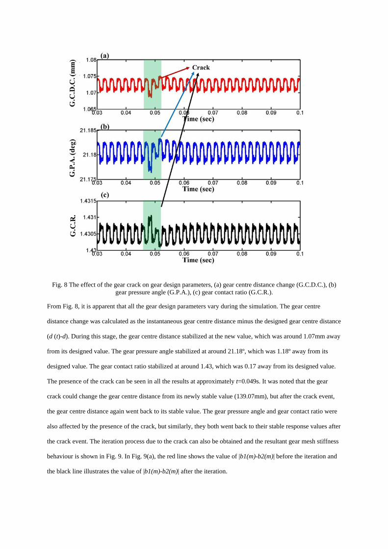
Fig. 8 The effect of the gear crack on gear design parameters, (a) gear centre distance change (G.C.D.C.), (b) gear pressure angle (G.P.A.), (c) gear contact ratio (G.C.R.).

From Fig. 8, it is apparent that all the gear design parameters vary during the simulation. The gear centre

distance change was calculated as the instantaneous gear centre distance minus the designed gear centre distance

(d (t)-d). During this stage, the gear centre distance stabilized at the new value, which was around 1.07mm away

from its designed value. The gear pressure angle stabilized at around 21.18º, which was 1.18º away from its

designed value. The gear contact ratio stabilized at around 1.43, which was 0.17 away from its designed value.

The presence of the crack can be seen in all the results at approximately t=0.049s. It was noted that the gear

crack could change the gear centre distance from its newly stable value (139.07mm), but after the crack event,

the gear centre distance again went back to its stable value. The gear pressure angle and gear contact ratio were

also affected by the presence of the crack, but similarly, they both went back to their stable response values after

the crack event. The iteration process due to the crack can also be obtained and the resultant gear mesh stiffness

behaviour is shown in Fig. 9. In Fig. 9(a), the red line shows the value of |b1(m)-b2(m)| before the iteration and

the black line illustrates the value of |b1(m)-b2(m)| after the iteration.

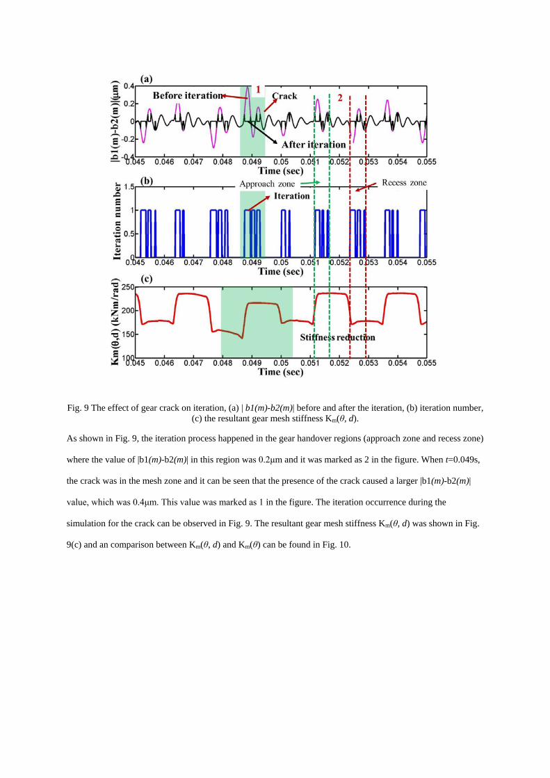
Fig. 9 The effect of gear crack on iteration, (a) | b1(m)-b2(m)| before and after the iteration, (b) iteration number, (c) the resultant gear mesh stiffness Km(θ, d).

As shown in Fig. 9, the iteration process happened in the gear handover regions (approach zone and recess zone)

where the value of |b1(m)-b2(m)| in this region was 0.2μm and it was marked as 2 in the figure. When t=0.049s,

the crack was in the mesh zone and it can be seen that the presence of the crack caused a larger |b1(m)-b2(m)|

value, which was 0.4μm. This value was marked as 1 in the figure. The iteration occurrence during the

simulation for the crack can be observed in Fig. 9. The resultant gear mesh stiffness Km(θ, d) was shown in Fig.

9(c) and an comparison between Km(θ, d) and Km(θ) can be found in Fig. 10.

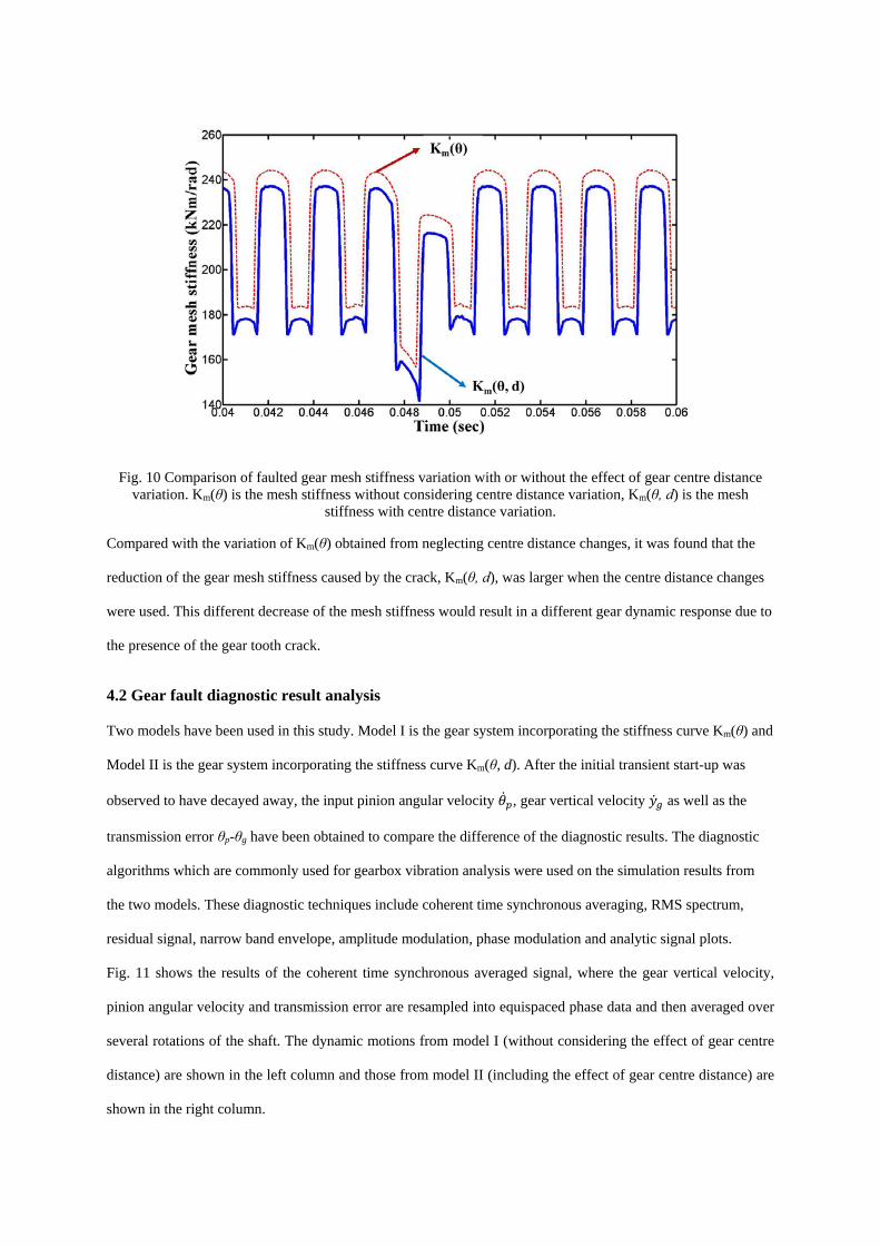
Fig. 10 Comparison of faulted gear mesh stiffness variation with or without the effect of gear centre distance variation. Km(θ) is the mesh stiffness without considering centre distance variation, Km(θ, d) is the mesh

stiffness with centre distance variation.

Compared with the variation of Km(θ) obtained from neglecting centre distance changes, it was found that the

reduction of the gear mesh stiffness caused by the crack, Km(θ, d), was larger when the centre distance changes

were used. This different decrease of the mesh stiffness would result in a different gear dynamic response due to

the presence of the gear tooth crack.

4.2 Gear fault diagnostic result analysis

Two models have been used in this study. Model I is the gear system incorporating the stiffness curve Km(θ) and

Model II is the gear system incorporating the stiffness curve Km(θ, d). After the initial transient start-up was

observed to have decayed away, the input pinion angular velocity �̇�𝜃𝑝𝑝, gear vertical velocity �̇�𝑦𝑔𝑔 as well as the

transmission error θp-θg have been obtained to compare the difference of the diagnostic results. The diagnostic

algorithms which are commonly used for gearbox vibration analysis were used on the simulation results from

the two models. These diagnostic techniques include coherent time synchronous averaging, RMS spectrum,

residual signal, narrow band envelope, amplitude modulation, phase modulation and analytic signal plots.

Fig. 11 shows the results of the coherent time synchronous averaged signal, where the gear vertical velocity,

pinion angular velocity and transmission error are resampled into equispaced phase data and then averaged over

several rotations of the shaft. The dynamic motions from model I (without considering the effect of gear centre

distance) are shown in the left column and those from model II (including the effect of gear centre distance) are

shown in the right column.

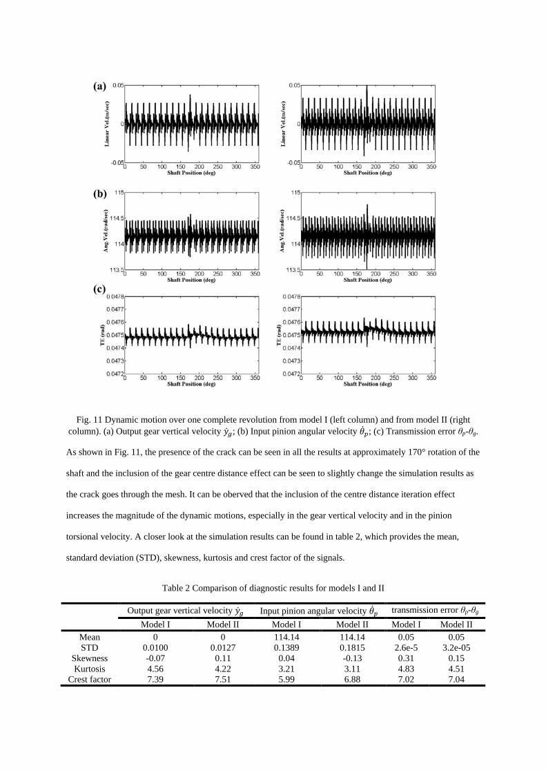
Fig. 11 Dynamic motion over one complete revolution from model I (left column) and from model II (right column). (a) Output gear vertical velocity �̇�𝑦𝑔𝑔; (b) Input pinion angular velocity �̇�𝜃𝑝𝑝; (c) Transmission error θp-θg.

As shown in Fig. 11, the presence of the crack can be seen in all the results at approximately 170° rotation of the

shaft and the inclusion of the gear centre distance effect can be seen to slightly change the simulation results as

the crack goes through the mesh. It can be oberved that the inclusion of the centre distance iteration effect

increases the magnitude of the dynamic motions, especially in the gear vertical velocity and in the pinion

torsional velocity. A closer look at the simulation results can be found in table 2, which provides the mean,

standard deviation (STD), skewness, kurtosis and crest factor of the signals.

Table 2 Comparison of diagnostic results for models I and II

Output gear vertical velocity �̇�𝑦𝑔𝑔 Input pinion angular velocity �̇�𝜃𝑝𝑝 transmission error θp-θg

Model I Model II Model I Model II Model I Model II Mean 0 0 114.14 114.14 0.05 0.05 STD 0.0100 0.0127 0.1389 0.1815 2.6e-5 3.2e-05

Skewness -0.07 0.11 0.04 -0.13 0.31 0.15 Kurtosis 4.56 4.22 3.21 3.11 4.83 4.51

Crest factor 7.39 7.51 5.99 6.88 7.02 7.04

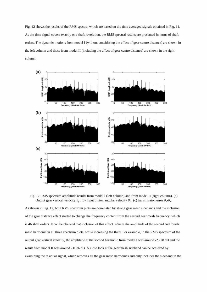
Fig. 12 shows the results of the RMS spectra, which are based on the time averaged signals obtained in Fig. 11.

As the time signal covers exactly one shaft revolution, the RMS spectral results are presented in terms of shaft

orders. The dynamic motions from model I (without considering the effect of gear centre distance) are shown in

the left column and those from model II (including the effect of gear centre distance) are shown in the right

column.

Fig. 12 RMS spectrum amplitude results from model I (left column) and from model II (right column). (a) Output gear vertical velocity �̇�𝑦𝑔𝑔; (b) Input pinion angular velocity �̇�𝜃𝑝𝑝; (c) transmission error θp-θg.

As shown in Fig. 12, both RMS spectrum plots are dominated by strong gear mesh sidebands and the inclusion

of the gear distance effect started to change the frequency content from the second gear mesh frequency, which

is 46 shaft orders. It can be oberved that inclusion of this effect reduces the amplitude of the second and fourth

mesh harmonic in all three spectrum plots, while increasing the third. For example, in the RMS spectrum of the

output gear vertical velocity, the amplitude at the second harmonic from model I was around -25.28 dB and the

result from model II was around -31.36 dB. A close look at the gear mesh sideband can be achieved by

examining the residual signal, which removes all the gear mesh harmonics and only includes the sideband in the

RMS spectra and then uses the inverse Fourier transform to obtain the signal in the time domain, as shown in

Fig. 13.

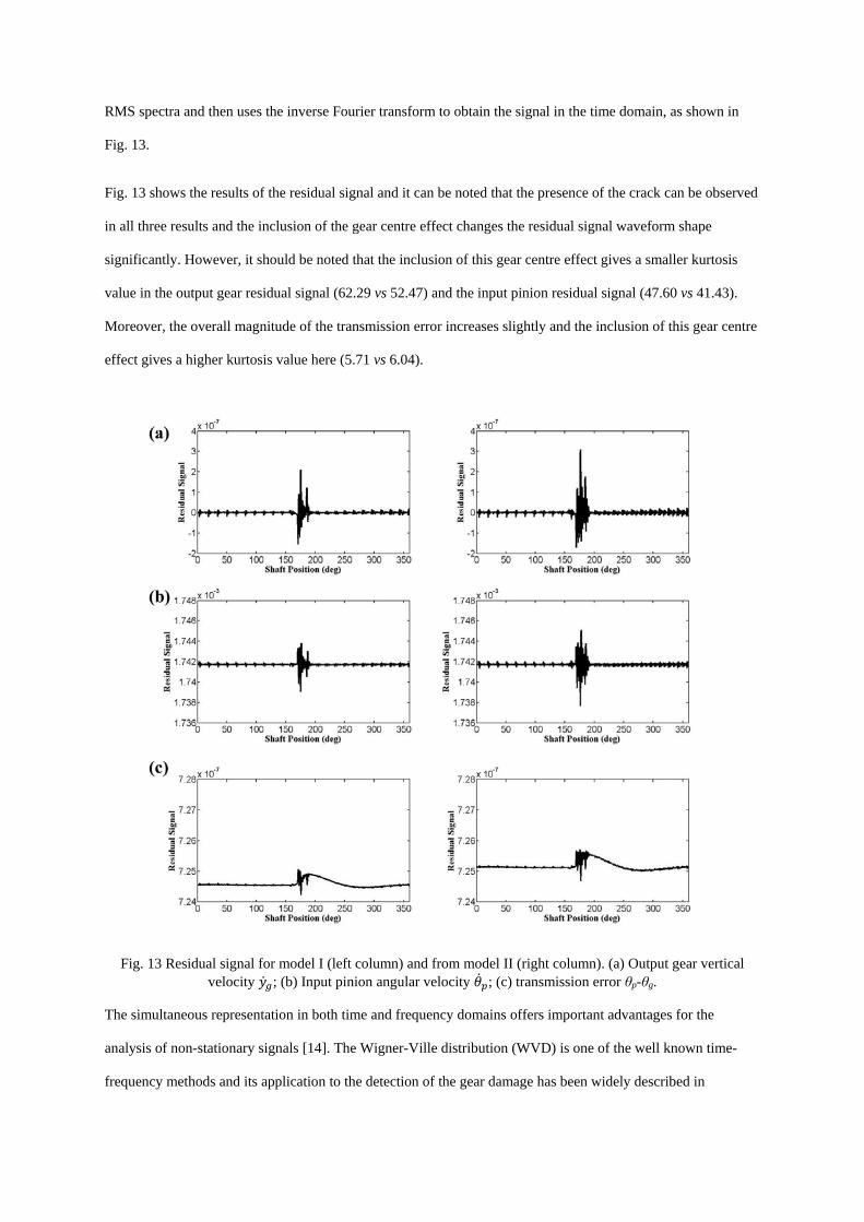
Fig. 13 shows the results of the residual signal and it can be noted that the presence of the crack can be observed

in all three results and the inclusion of the gear centre effect changes the residual signal waveform shape

significantly. However, it should be noted that the inclusion of this gear centre effect gives a smaller kurtosis

value in the output gear residual signal (62.29 vs 52.47) and the input pinion residual signal (47.60 vs 41.43).

Moreover, the overall magnitude of the transmission error increases slightly and the inclusion of this gear centre

effect gives a higher kurtosis value here (5.71 vs 6.04).

Fig. 13 Residual signal for model I (left column) and from model II (right column). (a) Output gear vertical velocity �̇�𝑦𝑔𝑔; (b) Input pinion angular velocity �̇�𝜃𝑝𝑝; (c) transmission error θp-θg.

The simultaneous representation in both time and frequency domains offers important advantages for the

analysis of non-stationary signals [14]. The Wigner-Ville distribution (WVD) is one of the well known time-

frequency methods and its application to the detection of the gear damage has been widely described in

publications [15]. By applying a suitable window function in the time domain, the cross-terms in the WVD can

be attenuated and the windowed version of the WVD is often called the pseudo Wigner-Ville distribution

(PWVD) [15]. In this research, the PWVD technique was employed to further compare the signals from model I

and model II. Note that the ‘shaft domain’ synchronous signal averages with the rotation ‘angle’ being

analogous to ‘time’ and the frequency was therefore in terms of shaft order [15].

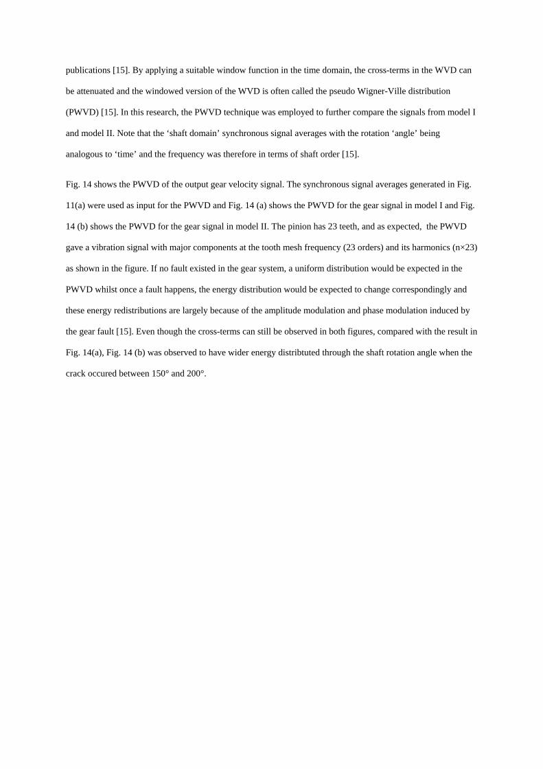
Fig. 14 shows the PWVD of the output gear velocity signal. The synchronous signal averages generated in Fig.

11(a) were used as input for the PWVD and Fig. 14 (a) shows the PWVD for the gear signal in model I and Fig.

14 (b) shows the PWVD for the gear signal in model II. The pinion has 23 teeth, and as expected, the PWVD

gave a vibration signal with major components at the tooth mesh frequency (23 orders) and its harmonics (n×23)

as shown in the figure. If no fault existed in the gear system, a uniform distribution would be expected in the

PWVD whilst once a fault happens, the energy distribution would be expected to change correspondingly and

these energy redistributions are largely because of the amplitude modulation and phase modulation induced by

the gear fault [15]. Even though the cross-terms can still be observed in both figures, compared with the result in

Fig. 14(a), Fig. 14 (b) was observed to have wider energy distribtuted through the shaft rotation angle when the

crack occured between 150° and 200°.

Fig. 14 The Pseudo Wigner-Ville distribution (PWVD) of the output gear vertical velocity �̇�𝑦𝑔𝑔, (a) PWVD of the signal from model I; (b) PWVD of the signal from model II.

The limitation of using the synchronous averaged signal for PWVD analysis was that the gear mesh harmonics

were found to dominate the distribution and removing the components at the meshing harmonics can increase

the sensitivity to energy changes related to the damage [16]. Further analysis can be found in Fig. 15, which

presents the PWVD analysis of the residual signal of the output gear vertical velocity �̇�𝑦𝑔𝑔. A much clearer

difference in the energy distribution pattern can be observed and these results further indicated that the highest

energy occurred around the fifth mesh harmonic.

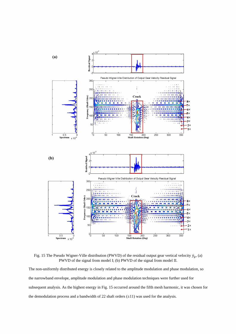
Fig. 15 The Pseudo Wigner-Ville distribution (PWVD) of the residual output gear vertical velocity �̇�𝑦𝑔𝑔, (a) PWVD of the signal from model I; (b) PWVD of the signal from model II.

The non-uniformly distributed energy is closely related to the amplitude modulation and phase modulation, so

the narrowband envelope, amplitude modulation and phase modulation techniques were further used for

subsequent analysis. As the highest energy in Fig. 15 occurred around the fifth mesh harmonic, it was chosen for

the demodulation process and a bandwidth of 22 shaft orders (±11) was used for the analysis.

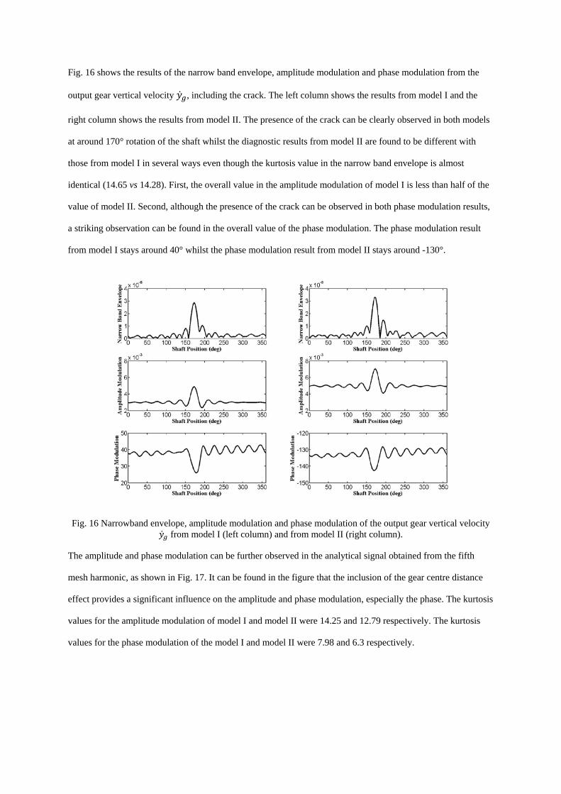
Fig. 16 shows the results of the narrow band envelope, amplitude modulation and phase modulation from the

output gear vertical velocity �̇�𝑦𝑔𝑔, including the crack. The left column shows the results from model I and the

right column shows the results from model II. The presence of the crack can be clearly observed in both models

at around 170° rotation of the shaft whilst the diagnostic results from model II are found to be different with

those from model I in several ways even though the kurtosis value in the narrow band envelope is almost

identical (14.65 vs 14.28). First, the overall value in the amplitude modulation of model I is less than half of the

value of model II. Second, although the presence of the crack can be observed in both phase modulation results,

a striking observation can be found in the overall value of the phase modulation. The phase modulation result

from model I stays around 40° whilst the phase modulation result from model II stays around -130°.

Fig. 16 Narrowband envelope, amplitude modulation and phase modulation of the output gear vertical velocity �̇�𝑦𝑔𝑔 from model I (left column) and from model II (right column).

The amplitude and phase modulation can be further observed in the analytical signal obtained from the fifth

mesh harmonic, as shown in Fig. 17. It can be found in the figure that the inclusion of the gear centre distance

effect provides a significant influence on the amplitude and phase modulation, especially the phase. The kurtosis

values for the amplitude modulation of model I and model II were 14.25 and 12.79 respectively. The kurtosis

values for the phase modulation of the model I and model II were 7.98 and 6.3 respectively.

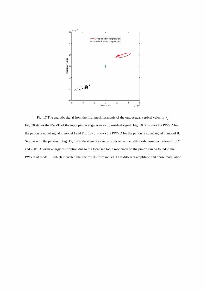
Fig. 17 The analytic signal from the fifth mesh harmonic of the output gear vertical velocity �̇�𝑦𝑔𝑔.

Fig. 18 shows the PWVD of the input pinion angular velocity residual signal. Fig. 18 (a) shows the PWVD for

the pinion residual signal in model I and Fig. 18 (b) shows the PWVD for the pinion residual signal in model II.

Similar with the pattern in Fig. 15, the highest energy can be observed at the fifth mesh harmonic between 150°

and 200°. A wider energy distribution due to the localised tooth root crack on the pinion can be found in the

PWVD of model II, which indicated that the results from model II has different amplitude and phase modulation.

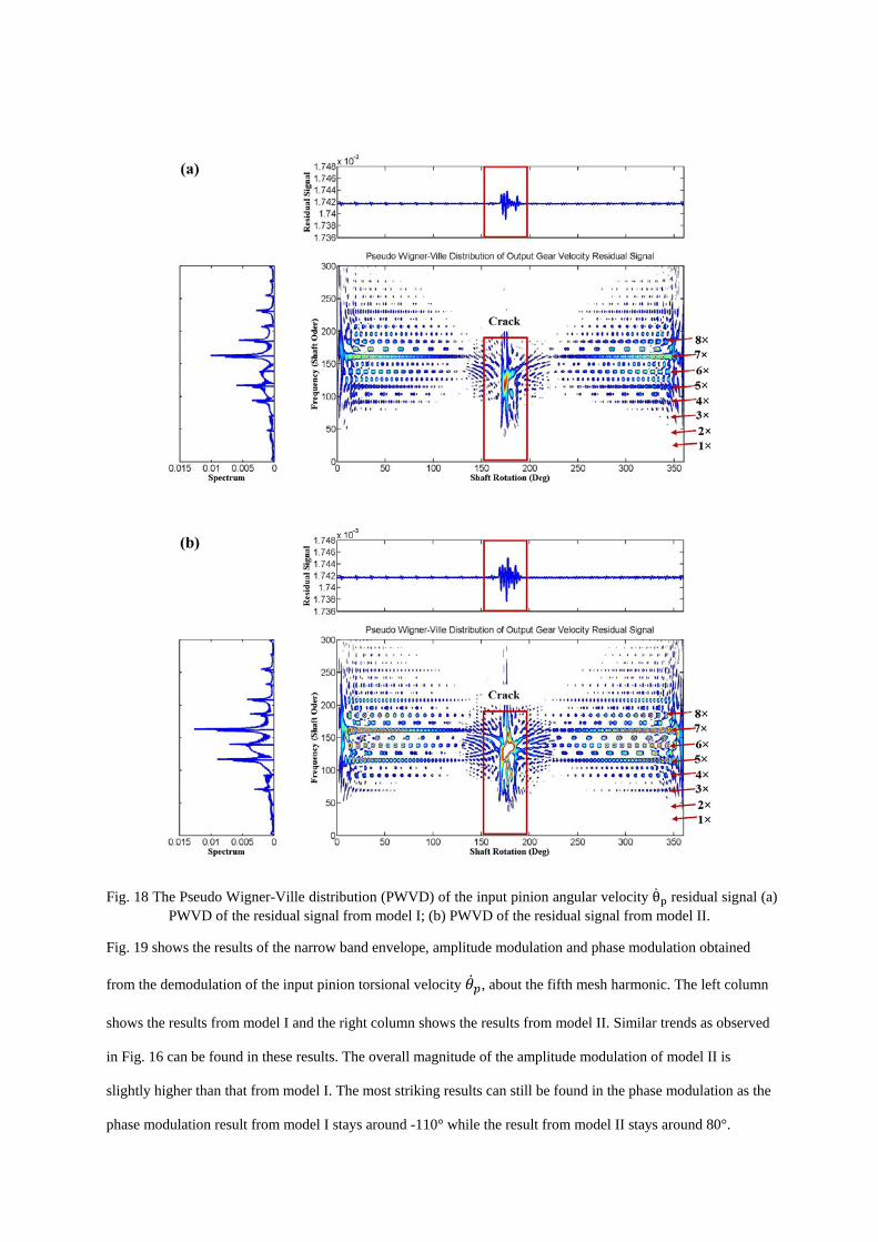
Fig. 18 The Pseudo Wigner-Ville distribution (PWVD) of the input pinion angular velocity θ̇p residual signal (a) PWVD of the residual signal from model I; (b) PWVD of the residual signal from model II.

Fig. 19 shows the results of the narrow band envelope, amplitude modulation and phase modulation obtained

from the demodulation of the input pinion torsional velocity �̇�𝜃𝑝𝑝, about the fifth mesh harmonic. The left column

shows the results from model I and the right column shows the results from model II. Similar trends as observed

in Fig. 16 can be found in these results. The overall magnitude of the amplitude modulation of model II is

slightly higher than that from model I. The most striking results can still be found in the phase modulation as the

phase modulation result from model I stays around -110° while the result from model II stays around 80°.

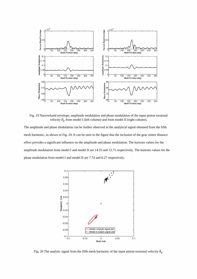
Fig. 19 Narrowband envelope, amplitude modulation and phase modulation of the input pinion torsional velocity �̇�𝜃𝑝𝑝 from model I (left column) and from model II (right column).

The amplitude and phase modulation can be further observed in the analytical signal obtained from the fifth

mesh harmonic, as shown in Fig. 20. It can be seen in the figure that the inclusion of the gear centre distance

effect provides a significant influence on the amplitude and phase modulation. The kurtosis values for the

amplitude modulation from model I and model II are 14.25 and 12.71 respectively. The kurtosis values for the

phase modulation from model I and model II are 7.74 and 6.27 respectively.

Fig. 20 The analytic signal from the fifth mesh harmonic of the input pinion torsional velocity �̇�𝜃𝑝𝑝.

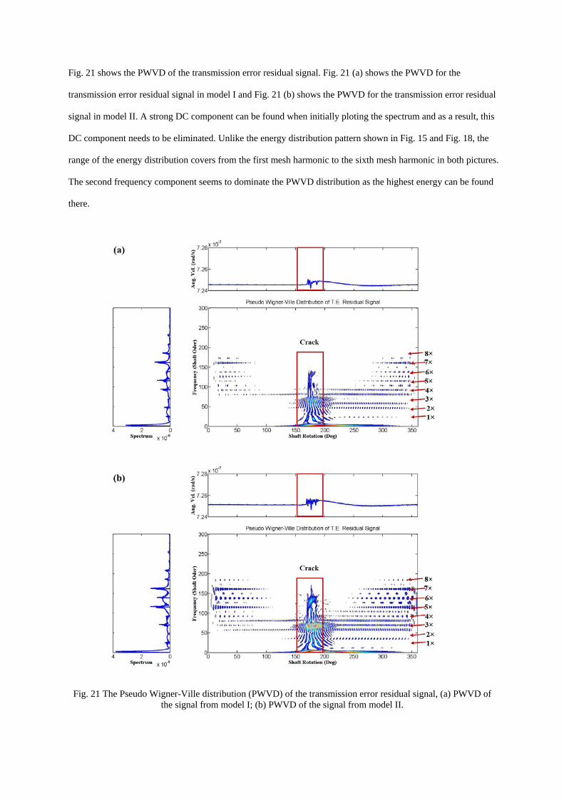
Fig. 21 shows the PWVD of the transmission error residual signal. Fig. 21 (a) shows the PWVD for the

transmission error residual signal in model I and Fig. 21 (b) shows the PWVD for the transmission error residual

signal in model II. A strong DC component can be found when initially ploting the spectrum and as a result, this

DC component needs to be eliminated. Unlike the energy distribution pattern shown in Fig. 15 and Fig. 18, the

range of the energy distribution covers from the first mesh harmonic to the sixth mesh harmonic in both pictures.

The second frequency component seems to dominate the PWVD distribution as the highest energy can be found

there.

Fig. 21 The Pseudo Wigner-Ville distribution (PWVD) of the transmission error residual signal, (a) PWVD of the signal from model I; (b) PWVD of the signal from model II.

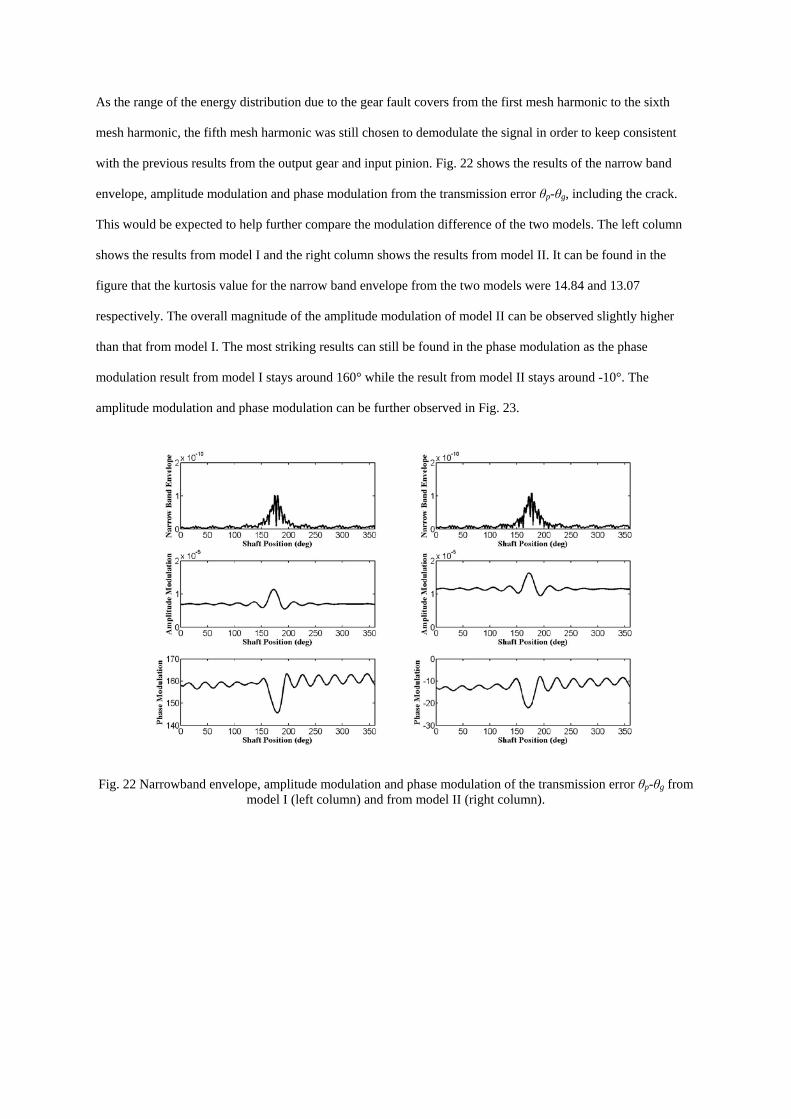
As the range of the energy distribution due to the gear fault covers from the first mesh harmonic to the sixth

mesh harmonic, the fifth mesh harmonic was still chosen to demodulate the signal in order to keep consistent

with the previous results from the output gear and input pinion. Fig. 22 shows the results of the narrow band

envelope, amplitude modulation and phase modulation from the transmission error θp-θg, including the crack.

This would be expected to help further compare the modulation difference of the two models. The left column

shows the results from model I and the right column shows the results from model II. It can be found in the

figure that the kurtosis value for the narrow band envelope from the two models were 14.84 and 13.07

respectively. The overall magnitude of the amplitude modulation of model II can be observed slightly higher

than that from model I. The most striking results can still be found in the phase modulation as the phase

modulation result from model I stays around 160° while the result from model II stays around -10°. The

amplitude modulation and phase modulation can be further observed in Fig. 23.

Fig. 22 Narrowband envelope, amplitude modulation and phase modulation of the transmission error θp-θg from model I (left column) and from model II (right column).

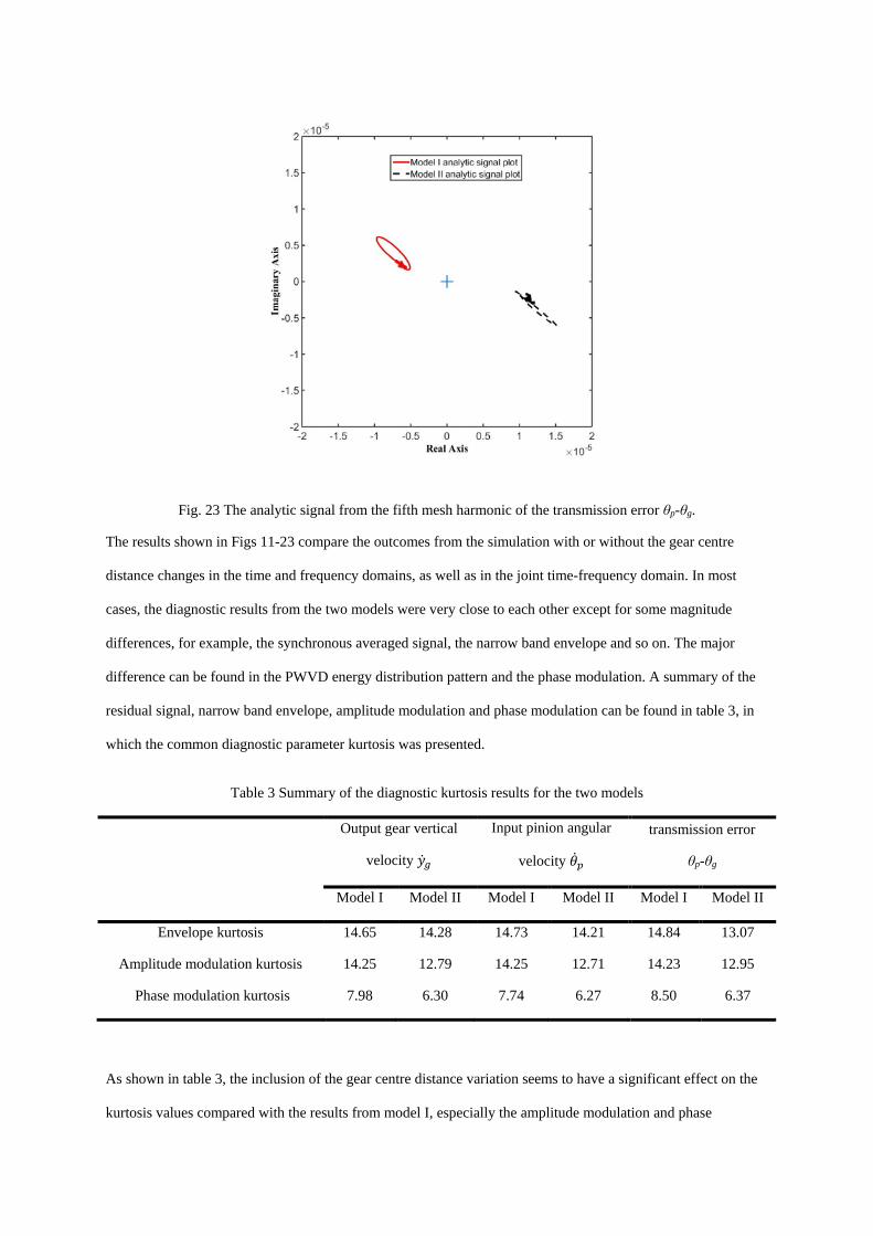
Fig. 23 The analytic signal from the fifth mesh harmonic of the transmission error θp-θg.

The results shown in Figs 11-23 compare the outcomes from the simulation with or without the gear centre

distance changes in the time and frequency domains, as well as in the joint time-frequency domain. In most

cases, the diagnostic results from the two models were very close to each other except for some magnitude

differences, for example, the synchronous averaged signal, the narrow band envelope and so on. The major

difference can be found in the PWVD energy distribution pattern and the phase modulation. A summary of the

residual signal, narrow band envelope, amplitude modulation and phase modulation can be found in table 3, in

which the common diagnostic parameter kurtosis was presented.

Table 3 Summary of the diagnostic kurtosis results for the two models

Output gear vertical

velocity �̇�𝑦𝑔𝑔

Input pinion angular

velocity �̇�𝜃𝑝𝑝

transmission error

θp-θg

Model I Model II Model I Model II Model I Model II

Envelope kurtosis 14.65 14.28 14.73 14.21 14.84 13.07

Amplitude modulation kurtosis 14.25 12.79 14.25 12.71 14.23 12.95

Phase modulation kurtosis 7.98 6.30 7.74 6.27 8.50 6.37

As shown in table 3, the inclusion of the gear centre distance variation seems to have a significant effect on the

kurtosis values compared with the results from model I, especially the amplitude modulation and phase

modulation kurtosis values while this inclusion appears to have negligible effect on the kurtosis values of the

narrow band envelope. The largest change with the inclusion of the gear centre distance in the presence of the

tooth crack occurred for the transmission error phase modulation kurtosis, where the kurtosis value decreased

from 8.50 to 6.37. In all cases, the introduction of the tooth crack gave a substantial decrease in the kurtosis

value with the inclusion of the gear centre distance.

5 Discussion

This paper has presented a method for improving the theoretical modelling of the flexible supported gears in

mesh by including the gear centre distance variation effect, which has a significant influence on the gear mesh

stiffness. The theoretical model has been kept simple in order to clearly show the effect of the gear centre

distance variation and therefore there are several major assumptions in the theoretical model itself, as

geometrical pitch, profile errors and ecentricity effects are neglected and the friction force between the teeth is

neglected. The account of any of these effects would change the resulting vibration response presented here, as

has been demonstrated by many authors [17, 18] while excluding these effects assists in focusing only on the

gear centre distance variation. Another major assumption is that the gear has been arranged in a way such that

the translational motion is restricted in the direction along the line of action. As a result, only the motion along

the line of action is included in the gear model. As demonstated in section 2, the gear centre distance can also

have influence on the pressure angle and this effect has been discussed by [9].

The Newmark method has been used to solve for the time domain reponses and an inspection at the end of each

time step was inserted to check the convergence of the system response. The important outcome of the

inspection is to improve the accuracy of the calculation. As this study has been focused on the impact of the gear

centre distance variation, the convergence criteria was based on the comparison of the gear centre distances

obtained from the previous and the current time step separately. A tolerance of 0.1μm was used for the

convergence criteria and by showing the iteration number at each time step, it was noted that the mesh stiffness

during the handover region as well as in the cracked region experienced modification by the iteration loop. This

was to be expected, as the mesh stiffness varies considerably with centre distance, as shown in Fig. 2 and Fig.

10. For a rigid bearing supported gear model where the gear centre distance only varies in a small range (for

example, less than 0.1μm), this inspection does not neccesarily improve the accuracy of the calculation, unless

some transient event was introduced to affect the gear centre distance.

The FEA method has been used to study the gear mesh stiffness curve by considering both the tooth root crack

and the gear centre distance changes. The reason for using the FEA method is that it was reported to be most

suitable for capturing the extended tooth contact phenomenon [19] as well as for modelling the gear tooth mesh

stiffness with larger gear tooth crack size [20]. As shown in Fig. 5 and Fig. 6, the FEA model was shown to

have a very good ability to capture both the root crack effect and the gear centre distance change effects.

The resultant gear vibration has been examined using some common gear diagnostic techniques in the time,

frequency and the joint time-frequency domain. Comparisons have been made between model I and model II in

these domains to investigate the effect of gear centre distance in the presence of the crack. In all cases, the

diagnostic techniques were able to clearly detect the presence of the crack in both models but with differences in

the magnitude and pattern. In the time domain, the properties of the time synchronous averaged results were

almost identical in both models as shown in table 2, except for the skewness parameter. In the frequency domain,

both spectrums are dominated by strong gear mesh harmonics and sidebands, though differences were observed

in the amplitudes of several of the gear mesh harmonics from the spectrum figure. However, a notable

difference can be observed in the kurtosis value of the residual signals if the gear mesh harmonics were

eliminated and only the gear mesh sidebands were considered. It can be found that the kurtosis values of model

II were all slightly smaller than those of model I, which suggested the residual distribution of model I was

sharper and this can also be observed directly from the figure. This observation is as expected, because the

inclusion of the gear centre distance would introduce extra stiffness reduction when the tooth with the crack

went through the mesh, and so the system in model II at this moment should momentarily speed up more and

induce a larger vibration response. In the time-frequency domain, it was found both models have similar

behaviour with the PWVD results in [21]. However, different energy distribution patterns were found in the

presence of the localised tooth cracks. As pattern recognition [22] or image processing techniques [23] were

often used to interpret the PWVD for detection of gear failure, the inclusion of the gear centre distance model is

expected to provide a more precise distribution, which can help better identify the failure. Significant phase

modulation, which was very similar to the results in [24], was found to occur when the crack was present in the

simulation. From the analytic signal plot, it can be found that the inclusion of the gear centre distance introduced

a completely different phase response in the signal compared with the phase response in model I. This is to be

expected as the inclusion of the gear centre distance can change the gear contact ratio and subsequently change

the length of the single and double contact zones, and so the system should change the speed-up duration in the

single contact zone and then the slowdown duration as the tooth enters the double contact zone.

6 Conclusion

This paper has demonstrated the major effect of the gear centre distance variation on the diagnostic response of

a gear tooth crack using a simplifed one stage gear dynamic model, where the geometrical error and eccentricity

effects have been neglected. The inclusion of the gear centre distance variation has been shown to change the

behaviour of the gear mesh stiffness curve, which has been incorporated into the gear dynamic model. The

iteration process proposed in the new gear dynamic model can reduce the errors caused by the gear centre

distance variation during the simulation and the resultant vibration behaviour can still clearly show the effect of

the presence of the crack. When comparing the diagnostic results from the previous model that neglected the

gear centre distance variation, it was seen that a notable difference can be observed, especially in the phase

modulation. All these data indicated that the effect of the gear centre distance variation has a significant effect

on the detection of the gear fault for the flexible supported gear. The iteration method used in this study

provides a possible way to improve the accuracy of gear dynamic modelling and hence further improve the

accuracy of gear fault diagnostic methods.

Acknowledgement

The funding support by China Scholarship Council (CSC) is greatly acknowledged.

Reference

[1] H. N. Ozguven, D. R. Houser, Mathematical models used in gear dynamics- a review, J. Sound Vib., 121(3)

(1988) 384-411.

[2] W. Bartelmus, Mathematical modelling and computer simulations as an aid to gearbox diagnostics, Mech.

Syst. Signal Proc., 15(5)(2001) 855-871.

[3] S. Du, Dynamic modelling and simulation of gear transmission error for gearbox vibration analysis,

University of New South Wales, Ph.D. Thesis, 1997.

[4] I. Howard, S. Jia, & J. Wang, The dynamic modelling of a spur gear in mesh including friction and a crack.

Mech. Syst. Signal Proc., 15(5)(2001) 831-853.

[5] S. Jia, I. Howard, Comparison of localised spalling and crack damage from dynamic modelling of spur gear

vibration. Mech. Syst. Signal Proc., 20(2)(2006) 332-349.

[6] F. Chaari, W. Baccar, M. S. Abbes, & M. Haddar, Effect of spalling or tooth breakage on gearmesh stiffness

and dynamic response of a one-stage spur gear transmission, Eur. J. Mech. A-Solid, 27(4)(2008) 691-705.

[7] D. P. Townsend. Dudley's Gear Handbook, second ed., Mcgraw-Hill, New York, 1992.

[8] H. H. Lin, C. Liou, & D. P. Townsend, Balancing Dynamic Strength of Spur Gears Operated at Extended

Center Distance, NASA Technical Memorandum 107222, 1996.

[9] W. Kim, H. H. Yoo, & J. Chung, Dynamic analysis for a pair of spur gears with translational motion due to

bearing deformation, J. Sound Vib., 329(21) (2010) 4409-4421.

[10] W. Kim, J. Y. Lee, & J. Chung, Dynamic analysis for a planetary gear with time-varying pressure angles

and contact ratios, J. Sound Vib., 331(4) (2012) 883-901.

[11] J. Wang, Numerical and experimental analysis of spur gears in mesh, Ph.D. thesis, Curtin University of

Technology, 2003.

[12] O. F. Chaari, T. Fakhfakh, & M. Haddar, Analytical modelling of spur gear tooth crack and influence on

gearmesh stiffness, Eur. J. Mech. A-Solid, 28 (2009) 461-468.

[13] S. Wu, M. Zuo, A. Parey, Simulation of spur gear dynamics and estimation of fault growth, J. Sound Vib.,

317 (2008) 608-624.

[14] L. Cohen. Time-frequency analysis, first ed., Prentice-Hall PTR, New Jersey, 1995.

[15] B.D. Forrester, Advanced vibration analysis techniques for fault detection and diagnosis in geared

transmission systems, Ph.D. thesis, Swinburne University of Technology, 1996.

[16] W.J. Wang, P.D, McFadden, Early detection of gear failure by vibration analysis—I. calculation of the

time-frequency distribution, Mech. Syst. Signal Proc., 7(3) (1993) 193-203.

[17] S. Jia, I. Howard, & J. Wang, The dynamic modeling of multiple pairs of spur gears in mesh, including

friction and geometrical errors, International Journal of Rotating Machinery, 9 (2003) 437-442.

[18] M. Inalpolat, M. Handschuh, & A. Kahraman, Influence of indexing errors on dynamic response of spur

gear pairs, Mech. Syst. Signal Proc., 60-61 (2015) 391-405.

[19] H. Ma, X. Pang, R. Feng, R. Song, & B. Wen, Fault features analysis of cracked gear considering the

effects of the extended tooth contact, Eng. Fail. Anal., 48 (2015) 105-120.

[20] O. Mohammed, M. Rantatalo, & J. Aidanpaa, Improving mesh stiffness calculation of cracked gears for the

purpose of vibration-based fault analysis, Eng. Fail. Anal., 34 (2013) 235-251.

[21] B.D. Forrester, Gear fault detection using the Wigner-Ville Distribution, Australian Vibration and Noise

Conference, Melbourne, Australia, September 18-20, 1990, 296-299.

[22] W.J. Staszewski, K. Worden, & G.R. Tomlinson, Time-frequency analysis in gearbox fault detection using

the Wigner-Ville distribution and pattern recognition, Mech. Syst. Signal Proc., 11(5) (1997) 673-692.

[23] W.J. Wang, P.D. McFadden, Early detection of gear failure by vibration analysis—II. Interpretation of the

time–frequency distribution using image processing techniques, Mech. Syst. Signal Proc., 7(3) (1993) 205-215.

[24] P. D. McFadden, Detecting fatigue cracks in gears by amplitude and phase demodulation of the meshing

vibration, J. Vib. Acoust, 108(2) (1986) 165-170.

Appendix A Nomenclature

The following nomenclatures were used in the gear system,

Ig: mass moment of inertia of the gear;

Im: mass moment of inertia of the motor;

Iout: mass moment of inertia of the output load;

Ip: mass moment of inertia of the pinion;

kxp, kyp: radial stiffness of the pinion;

kxg, kyg: radial stiffness of the gear;

K00, K05, K10: mesh stiffness when the gear centre distance increment is 0mm, 0.5mm, 1mm;

KC005, KC105: mesh stiffness with a 5 mm crack when the gear centre distance increment is 0mm and 5mm;

kcp: stiffness of the input coupling and shaft;

kcg: stiffness of the output coupling and shaft;

Km(θ), Km(θ, d): mesh stiffness without and with considering the gear centre distance change;

kmb: linear translation tooth stiffness along line of contact between pinion and gear;

L00, L05, L10: the load sharing ratios with 0 mm, 5mm, and 10mm gear centre distance increments;

mg: mass of the gear;

mp: mass of the pinion;

N: normal tooth contact force along the line of contact between pinion and gear;

p: relative mesh displacement.

qcg: damping of the output coupling and shaft;

qcp: damping of the input coupling and shaft;

qmb: linear translation tooth damping along line of contact between pinion and gear;

qstg: torsional damping of the gear;

qstp: torsional damping of the pinion;

qxg, qyg: radial damping of the gear;

qxp, qyp: radial damping of the pinion;

rap, rag: addendum radius of the pinion and the gear;

rp, rg: base radius of the pinion and the gear;

Tin: input motor torque;

Tout: output load torque;

xg: linear displacement of gear in the horizontal direction (the x direction);

xp: linear displacement of pinion in the horizontal direction (the x direction);

yg: linear displacement of gear in the vertical direction (the x direction);

yp: linear displacement of pinion in the vertical direction (the x direction);

θg: angular displacement of the gear;

θm: angular displacement of the motor;

θout: angular displacement of the output load;

θp: angular displacement of the pinion;

α: the designed pressure angle;

Appendix B

𝑀𝑀 =

⎣⎢⎢⎢⎢⎢⎡𝐼𝐼𝑚𝑚 0 0 0 0 00 𝑚𝑚𝑝𝑝 0 0 0 00 0 𝐼𝐼𝑝𝑝 0 0 00 0 0 𝑚𝑚𝑔𝑔 0 00 0 0 0 𝐼𝐼𝑔𝑔 00 0 0 0 0 𝐼𝐼𝑜𝑜𝑜𝑜𝑠𝑠⎦

⎥⎥⎥⎥⎥⎤

,

𝑥𝑥 = [𝜃𝜃𝑚𝑚,𝑦𝑦𝑝𝑝,𝜃𝜃𝑝𝑝,𝑦𝑦𝑔𝑔,𝜃𝜃𝑔𝑔,𝜃𝜃𝑜𝑜𝑜𝑜𝑠𝑠]𝑇𝑇,

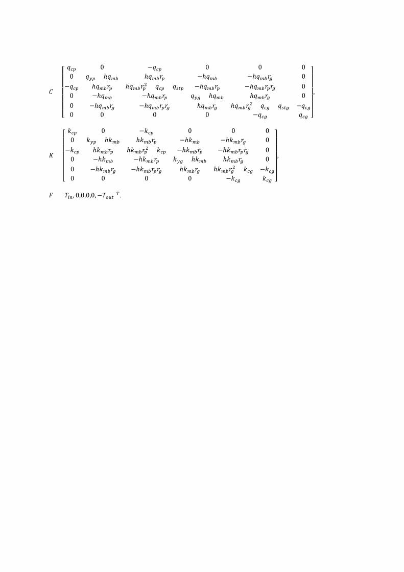
𝐶𝐶 =

⎣⎢⎢⎢⎢⎢⎡𝑞𝑞𝑐𝑐𝑝𝑝 0 −𝑞𝑞𝑐𝑐𝑝𝑝 0 0 00 𝑞𝑞𝑦𝑦𝑝𝑝 + ℎ𝑞𝑞𝑚𝑚𝑚𝑚 ℎ𝑞𝑞𝑚𝑚𝑚𝑚𝑟𝑟𝑝𝑝 −ℎ𝑞𝑞𝑚𝑚𝑚𝑚 −ℎ𝑞𝑞𝑚𝑚𝑚𝑚𝑟𝑟𝑔𝑔 0

−𝑞𝑞𝑐𝑐𝑝𝑝 ℎ𝑞𝑞𝑚𝑚𝑚𝑚𝑟𝑟𝑝𝑝 ℎ𝑞𝑞𝑚𝑚𝑚𝑚𝑟𝑟𝑝𝑝2 + 𝑞𝑞𝑐𝑐𝑝𝑝 + 𝑞𝑞𝑠𝑠𝑠𝑠𝑝𝑝 −ℎ𝑞𝑞𝑚𝑚𝑚𝑚𝑟𝑟𝑝𝑝 −ℎ𝑞𝑞𝑚𝑚𝑚𝑚𝑟𝑟𝑝𝑝𝑟𝑟𝑔𝑔 00 −ℎ𝑞𝑞𝑚𝑚𝑚𝑚 −ℎ𝑞𝑞𝑚𝑚𝑚𝑚𝑟𝑟𝑝𝑝 𝑞𝑞𝑦𝑦𝑔𝑔 + ℎ𝑞𝑞𝑚𝑚𝑚𝑚 ℎ𝑞𝑞𝑚𝑚𝑚𝑚𝑟𝑟𝑔𝑔 00 −ℎ𝑞𝑞𝑚𝑚𝑚𝑚𝑟𝑟𝑔𝑔 −ℎ𝑞𝑞𝑚𝑚𝑚𝑚𝑟𝑟𝑝𝑝𝑟𝑟𝑔𝑔 ℎ𝑞𝑞𝑚𝑚𝑚𝑚𝑟𝑟𝑔𝑔 ℎ𝑞𝑞𝑚𝑚𝑚𝑚𝑟𝑟𝑔𝑔2 + 𝑞𝑞𝑐𝑐𝑔𝑔 + 𝑞𝑞𝑠𝑠𝑠𝑠𝑔𝑔 −𝑞𝑞𝑐𝑐𝑔𝑔0 0 0 0 −𝑞𝑞𝑐𝑐𝑔𝑔 𝑞𝑞𝑐𝑐𝑔𝑔 ⎦

⎥⎥⎥⎥⎥⎤

,

𝐾𝐾 =

⎣⎢⎢⎢⎢⎢⎡𝑘𝑘𝑐𝑐𝑝𝑝 0 −𝑘𝑘𝑐𝑐𝑝𝑝 0 0 00 𝑘𝑘𝑦𝑦𝑝𝑝 + ℎ𝑘𝑘𝑚𝑚𝑚𝑚 ℎ𝑘𝑘𝑚𝑚𝑚𝑚𝑟𝑟𝑝𝑝 −ℎ𝑘𝑘𝑚𝑚𝑚𝑚 −ℎ𝑘𝑘𝑚𝑚𝑚𝑚𝑟𝑟𝑔𝑔 0

−𝑘𝑘𝑐𝑐𝑝𝑝 ℎ𝑘𝑘𝑚𝑚𝑚𝑚𝑟𝑟𝑝𝑝 ℎ𝑘𝑘𝑚𝑚𝑚𝑚𝑟𝑟𝑝𝑝2 + 𝑘𝑘𝑐𝑐𝑝𝑝 −ℎ𝑘𝑘𝑚𝑚𝑚𝑚𝑟𝑟𝑝𝑝 −ℎ𝑘𝑘𝑚𝑚𝑚𝑚𝑟𝑟𝑝𝑝𝑟𝑟𝑔𝑔 00 −ℎ𝑘𝑘𝑚𝑚𝑚𝑚 −ℎ𝑘𝑘𝑚𝑚𝑚𝑚𝑟𝑟𝑝𝑝 𝑘𝑘𝑦𝑦𝑔𝑔 + ℎ𝑘𝑘𝑚𝑚𝑚𝑚 ℎ𝑘𝑘𝑚𝑚𝑚𝑚𝑟𝑟𝑔𝑔 00 −ℎ𝑘𝑘𝑚𝑚𝑚𝑚𝑟𝑟𝑔𝑔 −ℎ𝑘𝑘𝑚𝑚𝑚𝑚𝑟𝑟𝑝𝑝𝑟𝑟𝑔𝑔 ℎ𝑘𝑘𝑚𝑚𝑚𝑚𝑟𝑟𝑔𝑔 ℎ𝑘𝑘𝑚𝑚𝑚𝑚𝑟𝑟𝑔𝑔2 + 𝑘𝑘𝑐𝑐𝑔𝑔 −𝑘𝑘𝑐𝑐𝑔𝑔0 0 0 0 −𝑘𝑘𝑐𝑐𝑔𝑔 𝑘𝑘𝑐𝑐𝑔𝑔 ⎦

⎥⎥⎥⎥⎥⎤

,

𝐹𝐹 = [𝑇𝑇𝑖𝑖𝑖𝑖, 0,0,0,0,−𝑇𝑇𝑜𝑜𝑜𝑜𝑠𝑠]𝑇𝑇.