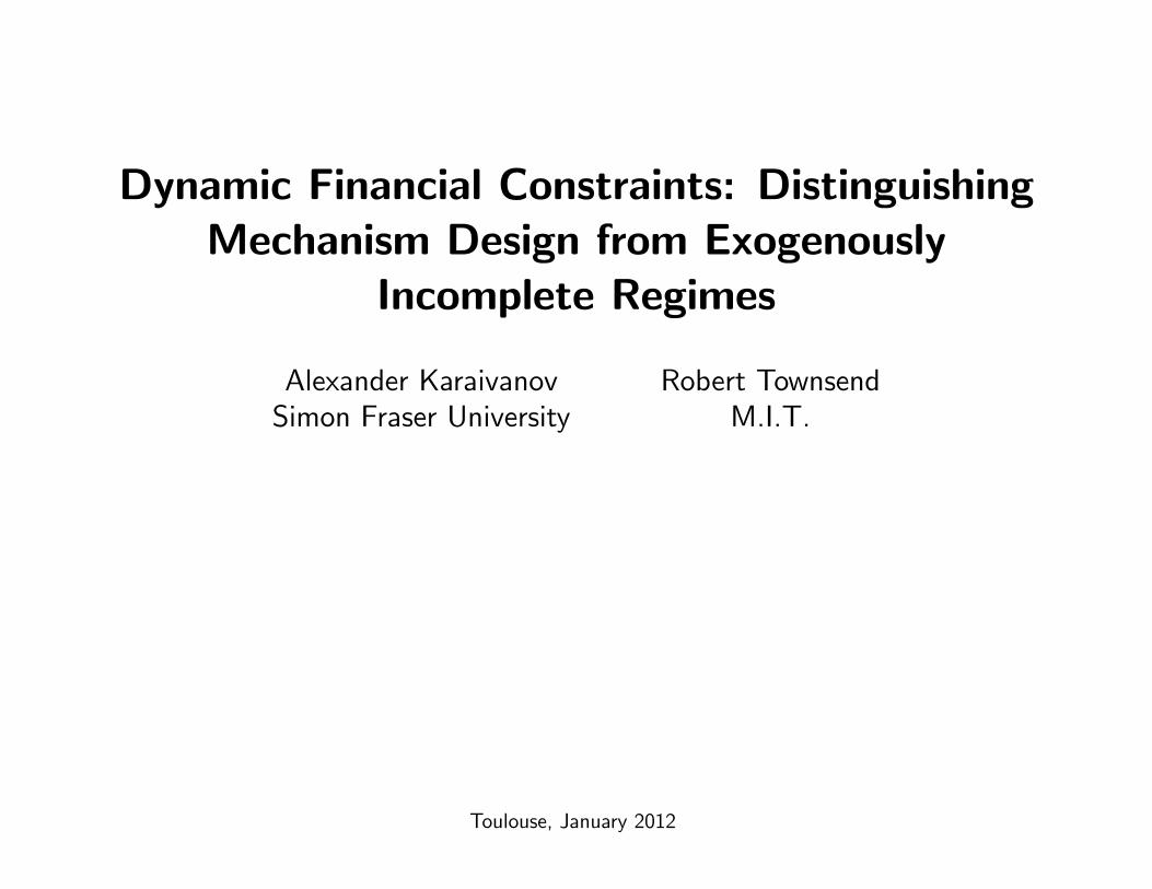
Dynamic Financial Constraints: DistinguishingMechanism Design from Exogenously

Incomplete Regimes

Alexander KaraivanovSimon Fraser University

Robert TownsendM.I.T.

Toulouse, January 2012

Karaivanov and Townsend Dynamic Financial Constraints

Literature on financial constraints: consumers vs. firmsdichotomy

• Consumption smoothing literature — various models with risk aversion— permanent income, buffer stock, full insurance

— private information (Phelan, 94, Ligon 98) or limited commitment(Thomas and Worrall, 90; Ligon et al., 05; Dubois et al., 08)

• Investment literature — firms modeled mostly as risk neutral— adjustment costs: Abel and Blanchard, 83; Bond and Meghir, 94

— IO (including structural): Hopenhayn, 92; Ericson & Pakes, 95,Cooley & Quadrini, 01; Albuquerque & Hopenhayn, 04; Clementi& Hopenhayn, 06; Schmid, 09

— empirical: e.g., Fazzari et al, 88 — unclear what the nature of financialconstraints is (Kaplan and Zingales, 00 critique); Samphantharak andTownsend, 10; Alem and Townsend, 10; Kinnan and Townsend, 11

Toulouse, January 2012 1

Karaivanov and Townsend Dynamic Financial Constraints

Literature (cont.)

• Macro literature with micro foundations

— largely assumes exogenously missing markets — Cagetti & De Nardi,06; Covas, 06; Angeletos and Calvet, 07; Heaton and Lucas, 00;Castro Clementi and Macdonald 09, Greenwood, Sanchez and Weage10a,b

• Comparing/testing across models of financial constraints —Meh andQuadrini 06; Paulson et al. 06; Jappelli and Pistaferri 06; Kocherlakotaand Pistaferri 07; Attanasio and Pavoni 08; Kinnan 09; Krueger andPerri 10; Krueger, Lustig and Perri 08 (asset pricing implications)

Toulouse, January 2012 2

Karaivanov and Townsend Dynamic Financial Constraints

Objectives

• how good an approximation are the various models of financial marketsaccess and constraints across the different literatures?

• what would be a reasonable assumption for the financial regime if it weretaken to the data as well?

— many ways in which markets can be incomplete

— financial constraints affect investment and consumption jointly (noseparation with incomplete markets)

— it matters what the exact source and nature of the constraints are

— can we distinguish and based on what and how much data?

Toulouse, January 2012 3

Karaivanov and Townsend Dynamic Financial Constraints

Contributions

• we solve dynamic models of incomplete markets — hard, but captures thefull implications of financial constraints

• we can handle any number of regimes with different frictions and anypreferences and technologies (no problems with non-convexities)

• using MLE we can estimate all structural parameters as opposed to onlya subset available using other methods (e.g., Euler equations)

• using MLE we capture in principle more (all) dimensions of the data(joint distribution of consumption, output, investment) as opposed toonly particular dimensions (e.g. consumption-output comovement; Eulerequations)

• structural approach allows computing counterfactuals, policy and welfareevaluations

Toulouse, January 2012 4

Karaivanov and Townsend Dynamic Financial Constraints

What we do

• formulate and solve a wide range of dynamic models/regimes of financialmarkets sharing common preferences and technology

— exogenously incomplete markets regimes — financial constraintsassumed / exogenously given (autarky, A; saving only, S; borrowing orlending in a single risk-free asset, B)

— mechanism-design (endogenously incomplete markets) regimes —financial constraints arise endogenously due to asymmetric information(moral hazard, MH; limited commitment, LC; hidden output;unobserved investment)

— complete markets (full information, FI)

Toulouse, January 2012 5

Karaivanov and Townsend Dynamic Financial Constraints

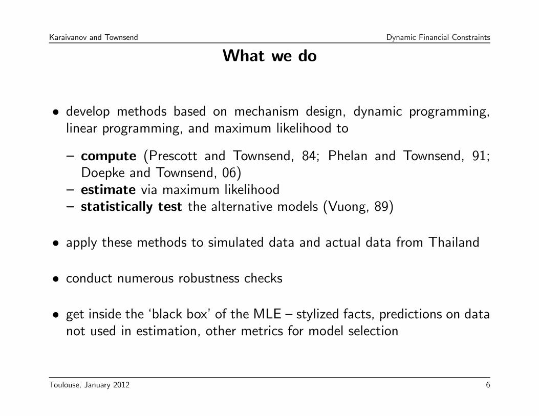
What we do

• develop methods based on mechanism design, dynamic programming,linear programming, and maximum likelihood to

— compute (Prescott and Townsend, 84; Phelan and Townsend, 91;Doepke and Townsend, 06)

— estimate via maximum likelihood— statistically test the alternative models (Vuong, 89)

• apply these methods to simulated data and actual data from Thailand

• conduct numerous robustness checks

• get inside the ‘black box’ of the MLE — stylized facts, predictions on datanot used in estimation, other metrics for model selection

Toulouse, January 2012 6

Karaivanov and Townsend Dynamic Financial Constraints

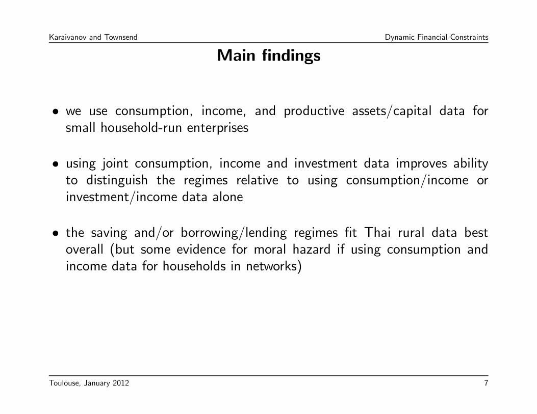
Main findings

• we use consumption, income, and productive assets/capital data forsmall household-run enterprises

• using joint consumption, income and investment data improves abilityto distinguish the regimes relative to using consumption/income orinvestment/income data alone

• the saving and/or borrowing/lending regimes fit Thai rural data bestoverall (but some evidence for moral hazard if using consumption andincome data for households in networks)

Toulouse, January 2012 7

Karaivanov and Townsend Dynamic Financial Constraints

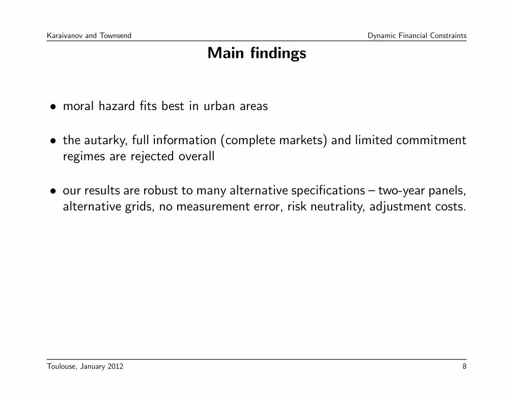
Main findings

• moral hazard fits best in urban areas

• the autarky, full information (complete markets) and limited commitmentregimes are rejected overall

• our results are robust to many alternative specifications — two-year panels,alternative grids, no measurement error, risk neutrality, adjustment costs.

Toulouse, January 2012 8

Karaivanov and Townsend Dynamic Financial Constraints

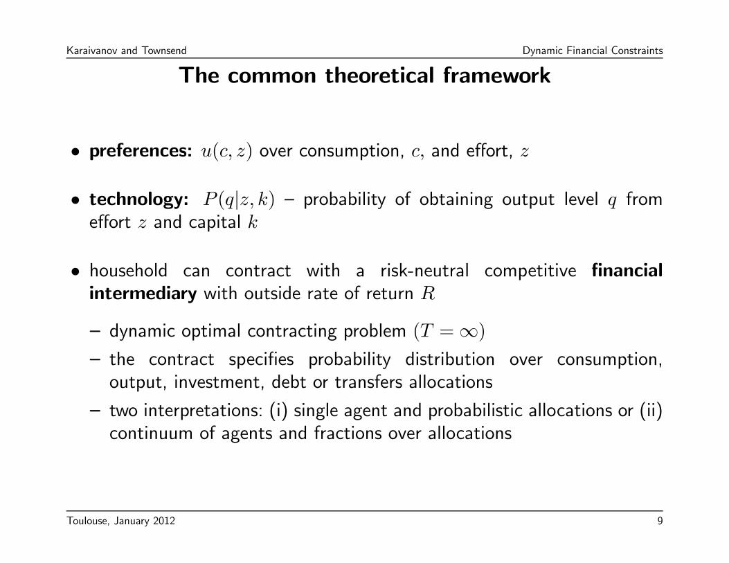
The common theoretical framework

• preferences: u(c, z) over consumption, c, and effort, z

• technology: P (q|z, k) — probability of obtaining output level q fromeffort z and capital k

• household can contract with a risk-neutral competitive financialintermediary with outside rate of return R

— dynamic optimal contracting problem (T =∞)— the contract specifies probability distribution over consumption,output, investment, debt or transfers allocations

— two interpretations: (i) single agent and probabilistic allocations or (ii)continuum of agents and fractions over allocations

Toulouse, January 2012 9

Karaivanov and Townsend Dynamic Financial Constraints

Timing

• initial state: k or (k,w) or (k, b) depending on the model regime (w ispromised utility, b is debt/savings)

• capital, k and effort, z used in production

• output, q realized, financial contract terms implemented (transfers, τ ornew debt/savings, b0)

• consumption, c and investment, i ≡ k0− (1− δ)k decided/implemented,

• go to next period state: k0, (k0, w0) or (k0, b0) depending on regime

Toulouse, January 2012 10

Karaivanov and Townsend Dynamic Financial Constraints

The linear programming (LP) approach

• we compute all models using linear programming

• write each model as dynamic linear program; all state and policy variablesbelong to finite grids, Z,K,W, T,Q,B, e.g. K = [0, .1, .5, 1]

• the choice variables are probabilities over all possible allocations(Prescott and Townsend, 84), e.g. π(q, z, k0, w0) ∈ [0, 1]

• extremely general formulation— by construction, no non-convexities for any preferences or technology(can be critical for MH, LC models)

— very suitable for MLE — direct mapping to probabilities— contrast with the “first order approach” — need additional restrictiveassumptions (Rogerson, 85; Jewitt, 88) or to verify solutionsnumerically (Abraham and Pavoni, 08)

Toulouse, January 2012 11

Karaivanov and Townsend Dynamic Financial Constraints

Example with the autarky problem

• “standard” formulation

v(k) = maxz,k0i

#Qi=1

Xqi∈Q

P (qi|k, z)[u(qi + (1− δ)k − k0i, z) + βv(k0i)]

• linear programming formulation

v(k) = maxπ(q,z,k0|k)≥0

QxZxK0π(q, z, k0|k)[u(q + (1− δ)k − k0, z) + βv(k0)]

s.t.

K0π(q, z, k0|k) = P (q|z, k)

Q×Kπ(q, z, k0|k) for all (q, z) ∈ Q× Z

QxZxK0π(q, z, k0|k) = 1

Toulouse, January 2012 12

Karaivanov and Townsend Dynamic Financial Constraints

Exogenously incomplete markets models (B, S, A)

• no information asymmetries; no default

• The agent’s problem:

v(k, b) = maxπ(q,z,k0,b0|k,b)

QxZxK0xB0π(q, z, k0, b0|k, b)[U(q+b0−Rb+(1−δ)k−k0, z)+βv(k0, b0)]

subject to Bayes-rule consistency and adding-up:

K0xB0π(q, z, k0, b0|k, b) = P (q|z, k)

Q×K0xB0π(q, z, k0, b0|k, b) for all (q, z) ∈ Q×Z

QxZxK0×B0π(q, z, k0, b0|k, b) = 1

and s.t. π(q, z, k0, b0|k, b) ≥ 0, ∀(q, z, k0, b0) ∈ Q× Z ×K0 ×B0

• autarky : set B0 = 0; saving only: set bmax = 0; debt : allow bmax > 0

Toulouse, January 2012 13

Karaivanov and Townsend Dynamic Financial Constraints

Mechanism design models (FI, MH, LC)

• allow state- and history-contingent transfers, τ

• dynamic optimal contracting problem between a risk-neutral lender andthe household

V (w, k) = maxπ(τ,q,z,k0,w0|k,w)

T×Q×Z×K0×W 0π(τ, q, z, k0, w0|k,w)[q−τ+(1/R)V (w0, k0)]

s.t. promise-keeping:XT×Q×Z×K0×W 0

π(τ , q, z, k0, w0|k,w)[U(τ +(1− δ)k− k0, z)+βw0] = w,

and s.t. Bayes-rule consistency, adding-up, and non-negativity as before.

Toulouse, January 2012 14

Karaivanov and Townsend Dynamic Financial Constraints

Moral hazard

• additional constraints — incentive-compatibility, ∀(z, z) ∈ Z × Z

T×Q×K0×W 0π(τ, q, z, k0, w0|k,w)[U(τ + (1− δ)k − k0, z) + βw0

] ≥

≥T×Q×K0×W 0

π(τ, q, z, k0, w0|k,w)P (q|z, k)P (q|z, k)

[U(τ + (1− δ)k − k0, z) + βw0]

• we also compute a moral hazard model with unobserved k and k0 (UI) —adds dynamic adverse selection as source of financial constraints

Toulouse, January 2012 15

Karaivanov and Townsend Dynamic Financial Constraints

Limited commitment

• additional constraints — limited commitment, for all (q, z) ∈ Q× Z

XT×K0×W 0

π(τ , q, z, k0, w0|k,w)[u(τ + (1− δ)k − k0, z) + βw0] ≥ Ω(k, q, z)

where Ω(k, q, z) is the present value of the agent going to autarky with hiscurrent output at hand q and capital k, which is defined as:

Ω(k, q, z) ≡ maxk0∈K0

u(q + (1− δ)k − k0, z) + βvaut(k0)

where vaut(k) is the autarky-forever value (from the A regime).

Toulouse, January 2012 16

Karaivanov and Townsend Dynamic Financial Constraints

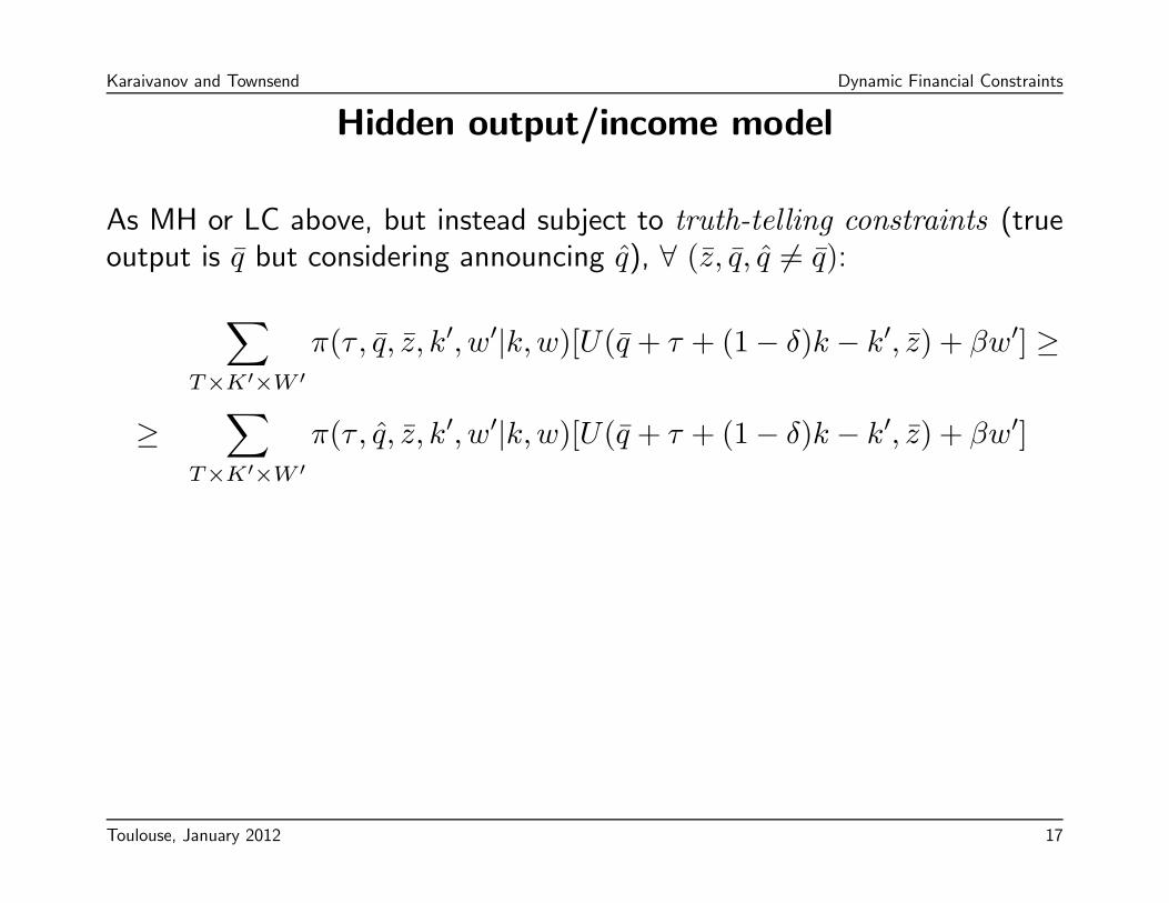
Hidden output/income model

As MH or LC above, but instead subject to truth-telling constraints (trueoutput is q but considering announcing q), ∀ (z, q, q 6= q):X

T×K0×W 0π(τ , q, z, k0, w0|k,w)[U(q + τ + (1− δ)k − k0, z) + βw0] ≥

≥X

T×K0×W 0π(τ , q, z, k0, w0|k,w)[U(q + τ + (1− δ)k − k0, z) + βw0]

Toulouse, January 2012 17

Karaivanov and Townsend Dynamic Financial Constraints

Functional forms and baseline parameters

• preferences:u(c, z) =

c1−σ

1− σ− ξzθ

• technology: calibrated from data (robustness check withparametric/estimated), the matrix P (q|z, k) for all q, z, k ∈ Q× Z ×K

• fixed parameters: β = .95, δ = .05, R = 1.053, ξ = 1 (the rest areestimated in the MLE; we also do robustness checks)

Toulouse, January 2012 18

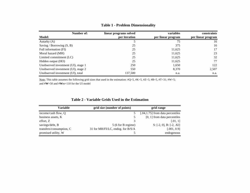
Number of: linear programs solved variables constraintsModel: per iteration per linear program per linear programAutarky (A) 5 75 16Saving / Borrowing (S, B) 25 375 16Full information (FI) 25 11,625 17Moral hazard (MH) 25 11,625 23Limited commitment (LC) 25 11,625 32Hidden output (HO) 25 11,625 77Unobserved investment (UI), stage 1 250 1,650 122Unobserved investment (UI), stage 2 550 8,370 2,507Unobserved investment (UI), total 137,500 n.a. n.a.

Note: This table assumes the following grid sizes that used in the estimation: #Q=5, #K=5, #Z=3, #B=5, #T=31; #W=5;and #W=50 and #Wm=110 for the UI model

Variable grid size (number of points) grid range

income/cash flow, Q 5 [.04,1.75] from data percentilesbusiness assets, K 5 [0, 1] from data percentileseffort, Z 3 [.01, 1]savings/debt, B 5 (6 for B regime) S: [-2, 0], B: [-2, .82]transfers/consumption, C 31 for MH/FI/LC, endog. for B/S/A [.001, 0.9]promised utility, W 5 endogenous

Table 1 - Problem Dimensionality

Table 2 - Variable Grids Used in the Estimation

Karaivanov and Townsend Dynamic Financial Constraints

Computation

• compute each model using policy function iteration (Judd 98)

• in general, let the initial state s be distributed D0(s) over the grid S (inthe estimations we use the k distribution from the data)

— use the LP solutions, π∗(.|s) to create the state transition matrix,M(s, s0) with elements mss0s,s0∈S

— for example, for MH s = (w, k) and thus

mss0 ≡ prob(w0, k0|w, k) =

T×Q×Zπ∗(τ, q, z, k0, w0|w, k)

the state distribution at time t is thus Dt(s) = (M0)tD0(s)

• use D(s), M(s, s0) and π∗(.|s) to generate cross-sectional distributions,time series or panels of any model variables

Toulouse, January 2012 19

Karaivanov and Townsend Dynamic Financial Constraints

Structural estimation

• Given:

— structural parameters, φs (to be estimated),— discretized over the grid K (observable state) distribution H(k)— the unobservable state (b or w) distribution — parameterized by φd

and estimated

• compute the conditional probability, gm1 (y|k, φs, φd) of any y = (c, q) ory = (k, i, q) or y = (c, q, i, k) implied by the solution π∗(.) of modelregime, m (m is A through FI), integrating over unobservable statevariables.

Toulouse, January 2012 20

Karaivanov and Townsend Dynamic Financial Constraints

Structural estimation

• allow for measurement error in k (Normal with stdev γme assumed inbaseline)

• use a histogram function over the state grid K to generate the modeljoint probability distribution fm(y|H(k), φs, φd, γme) given the statedistribution H(k).

• estimated parameters determining the likelihood, φ ≡ (φs, φd, γme)

Toulouse, January 2012 21

Karaivanov and Townsend Dynamic Financial Constraints

The likelihood function

Illustration:

• consider the case of y ≡ (c, q), i.e., cross-sectional data cj, qjnj=1. TheC ×Q grid used in the LP consists of the points ch, ql#K, #Q

h=1,l=1 .

• from above,fm(ch, ql|H(k), φ)

are the model m solution probabilities (obtained from the π’s andallowing measurement error in k) at each grid point ch, ql givenparameters φs, φd and initial observed state distribution H(k). Byconstruction,

Ph,l f

m(ch, ql|H(k), φ) = 1.

• suppose cj = c∗j + εcj and qj = q∗j + εqj where εc and εq are independent

Normal random variables with mean zero and normalized standarddeviations σc and σq (i.e., σc = γme(cmax − cmin) and similarly for q).Let Φ(.|μ, σ2) denote the Normal pdf.

Toulouse, January 2012 22

Karaivanov and Townsend Dynamic Financial Constraints

The likelihood function (cont.)

• ...then, the likelihood of data point (cj, qj) relative to any given gridpoint (c, q) ∈ C ×Q given φ,H(k) is:

Φ(cj|c, σ2c)Φ(qj|q, σ2q)

• the likelihood of data point (cj, qj) relative to the whole LP grid C ×Qis, adding over all grid points ch, ql with their probability weights fmimplied by model m:

Fm(cj, qj|φ,H(k)) =Xh

Xl

fm(ch, ql|H(k), φ)Φ(cj|ch, σ2c)Φ(qj|ql, σ2q)

Toulouse, January 2012 23

Karaivanov and Townsend Dynamic Financial Constraints

The likelihood function (cont.)

• therefore, the log-likelihood of the data cj, qjnj=1 in model m given φand H(k) and allowing for measurement error in k, c, q is:

Λm(φ) =nXj=1

lnFm(cj, qj|φ,H(k))

• in the runs with real data we use H(k) = H(k) — the discretizeddistribution of actual capital stock data kjnj=1.

Toulouse, January 2012 24

Karaivanov and Townsend Dynamic Financial Constraints

Structural estimation (cont.)

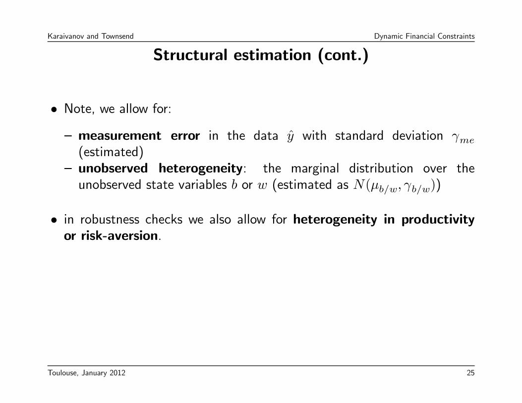
• Note, we allow for:

— measurement error in the data y with standard deviation γme

(estimated)— unobserved heterogeneity: the marginal distribution over theunobserved state variables b or w (estimated as N(μb/w, γb/w))

• in robustness checks we also allow for heterogeneity in productivityor risk-aversion.

Toulouse, January 2012 25

Karaivanov and Townsend Dynamic Financial Constraints

Testing

• Vuong’s (1989) modified likelihood ratio test

— neither model has to be correctly specified

— the null hypothesis is that the compared models are ‘equally close’ inKLIC sense to the data

— the test statistic is distributed N(0, 1) under the null

Toulouse, January 2012 26

Karaivanov and Townsend Dynamic Financial Constraints

Application to Thai data

• Townsend Thai Surveys (16 villages in four provinces, Northeast andCentral regions)

— balanced panel of 531 rural households observed 1999-2005 (sevenyears of data)

— balanced panel of 475 urban households observed 2005-2009

• data series used in estimation and testing

— consumption expenditure (c) — household-level, includes owner-produced consumption (fish, rice, etc.)

— assets (k) — used in production; include business and farm equipment,exclude livestock and household durables

— income (q) — measured on accrual basis (Samphantharak andTownsend, 09)

— investment (i) — constructed from assets data, i ≡ k0 − (1− δ)k

Toulouse, January 2012 27

24

6

100200

300400

500

−1000

0

1000

2000

3000

4000

year (1 = 1999)

rural data, income

household #devi

atio

ns fr

om y

ear

aver

age

99−

05, ’

000

baht

24

6

100200

300400

500

−1000

0

1000

2000

3000

4000

rural data, consumption

24

6

100200

300400

500

−1000

0

1000

2000

3000

4000

rural data, investment

2

4200

400

0

5000

10000

15000

year (1 = 2005)

urban data, income

household #

devi

atio

ns fr

om y

ear

aver

age

05−

09, ’

000

baht

2

4200

400

0

5000

10000

15000

urban data, consumption

12

34

200

400

0

5000

10000

15000

urban data, investment

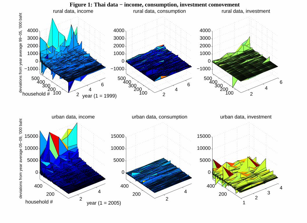
Figure 1: Thai data − income, consumption, investment comovement

−400 −200 0 200 400−400

−300

−200

−100

0

100

200

300

400

annual income changes, dy (’000 baht)

annu

al in

com

e an

d co

nsum

ptio

n ch

ange

s, d

c (’0

00 b

aht)

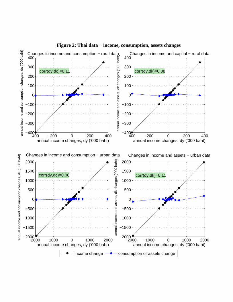
Changes in income and consumption − rural data

corr(dy,dc)=0.11

−400 −200 0 200 400−400

−300

−200

−100

0

100

200

300

400

annual income changes, dy (’000 baht)

annu

al in

com

e an

d as

sets

, dk

chan

ges

(’000

bah

t) Changes in income and capital − rural data

corr(dy,dk)=0.08

−2000 −1000 0 1000 2000−2000

−1500

−1000

−500

0

500

1000

1500

2000

annual income changes, dy (’000 baht)

annu

al in

com

e an

d co

nsum

ptio

n ch

ange

s, d

c (’0

00 b

aht) Changes in income and consumption − urban data

corr(dy,dc)=0.08

−2000 −1000 0 1000 2000−2000

−1500

−1000

−500

0

500

1000

1500

2000

annual income changes, dy (’000 baht)

annu

al in

com

e an

d as

sets

, dk

chan

ges

(’000

bah

t)

Changes in income and assets − urban data

corr(dy,dk)=0.11

income change consumption or assets change

Figure 2: Thai data − income, consumption, assets changes

Rural data, 1999-2005 Urban data, 2005-2009

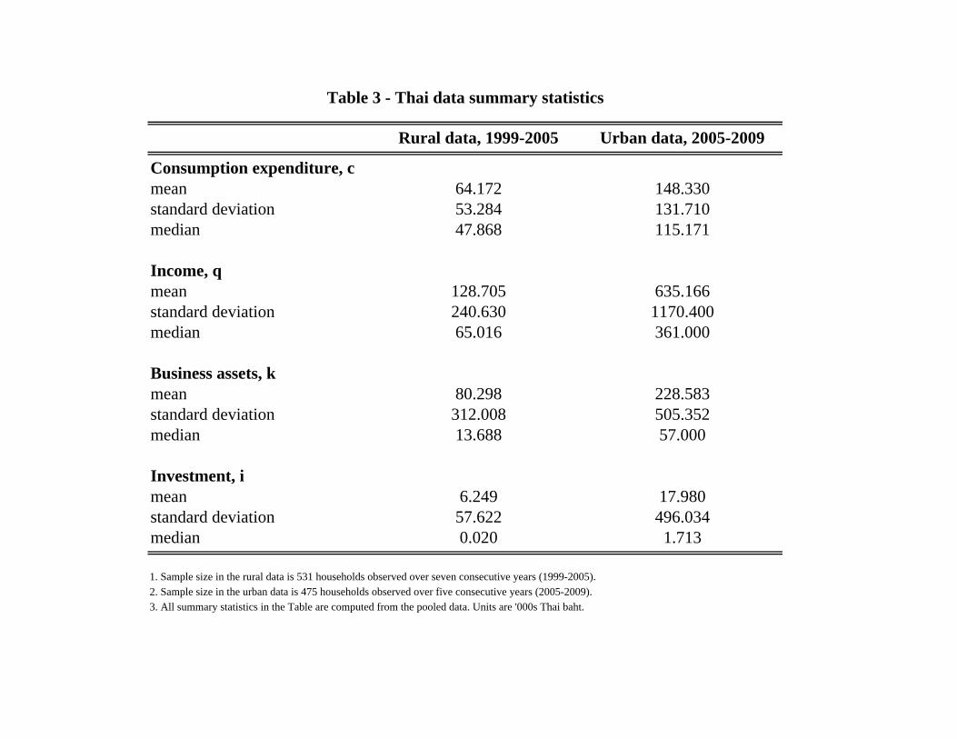
Consumption expenditure, cmean 64.172 148.330standard deviation 53.284 131.710median 47.868 115.171

Income, qmean 128.705 635.166standard deviation 240.630 1170.400median 65.016 361.000

Business assets, kmean 80.298 228.583standard deviation 312.008 505.352median 13.688 57.000

Investment, imean 6.249 17.980standard deviation 57.622 496.034median 0.020 1.713

1. Sample size in the rural data is 531 households observed over seven consecutive years (1999-2005).2. Sample size in the urban data is 475 households observed over five consecutive years (2005-2009).3. All summary statistics in the Table are computed from the pooled data. Units are '000s Thai baht.

Table 3 - Thai data summary statistics

Karaivanov and Townsend Dynamic Financial Constraints

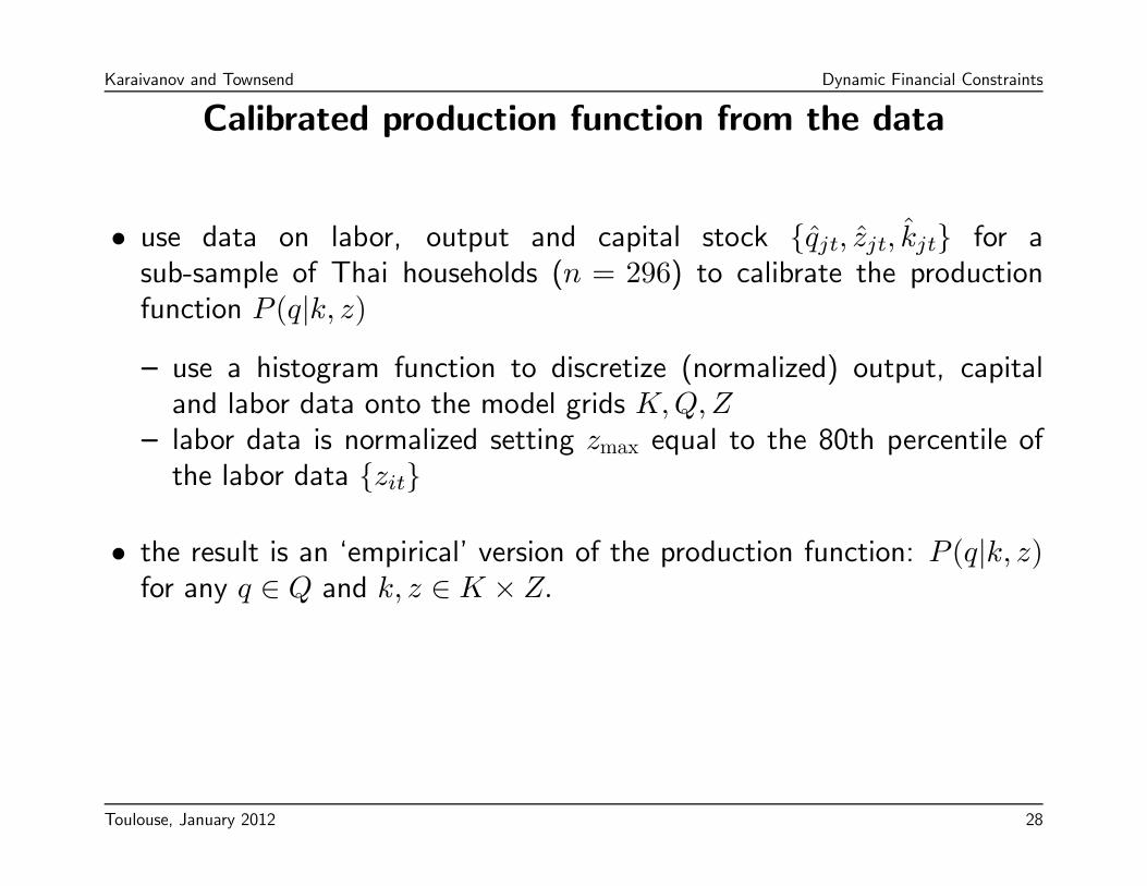
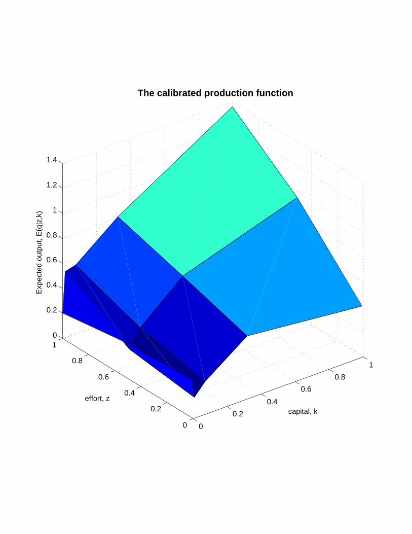
Calibrated production function from the data

• use data on labor, output and capital stock qjt, zjt, kjt for asub-sample of Thai households (n = 296) to calibrate the productionfunction P (q|k, z)

— use a histogram function to discretize (normalized) output, capitaland labor data onto the model grids K,Q,Z

— labor data is normalized setting zmax equal to the 80th percentile ofthe labor data zit

• the result is an ‘empirical’ version of the production function: P (q|k, z)for any q ∈ Q and k, z ∈ K × Z.

Toulouse, January 2012 28

0

0.2

0.4

0.6

0.8

1

0

0.2

0.4

0.6

0.8

10

0.2

0.4

0.6

0.8

1

1.2

1.4

capital, k

The calibrated production function

effort, z

Exp

ecte

d ou

tput

, E(q

|z,k

)

Karaivanov and Townsend Dynamic Financial Constraints

Application to Thai data (cont.)

• mapping to the model

— convert data into ‘model units’ — divide all nominal values by the 90%asset percentile

— draw initial unobserved states (w, b) from N(μw/b, γw/b); initial assetsk are taken from the data

— allow for additive measurement error in k, i, c, q (standard deviation,γme estimated)

• estimate and test pairwise the MH, LC, FI, B, S, A models with theThai data

Toulouse, January 2012 29

Karaivanov and Townsend Dynamic Financial Constraints

Thai data — results

• the exogenously incomplete markets S and B regimes fit the rural Thaidata best overall (Table 5)

— independent of type of data used (only exception is 1999 c, q data)— consistent with other evidence for imperfect risk-sharing andinvestment sensitivity to cash flow/income

• using joint consumption, income and investment data pins downthe best fitting regimes more sharply than consumption/income orinvestment/income data alone

• the full information (complete markets) (FI) and limited commitment(LC) regimes are rejected with all types of data (one exception)

• the autarky (A) (no access to financial markets) regime is rejected too

Toulouse, January 2012 30

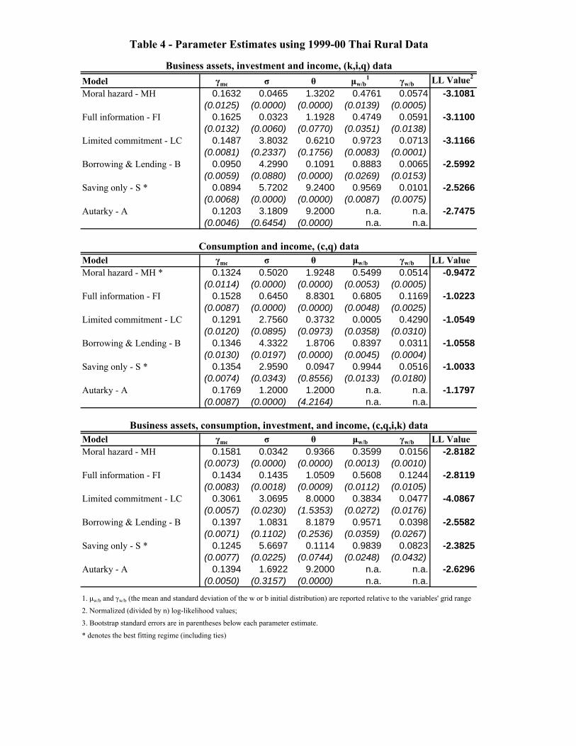
Model γme σ θ μw/b1 γw/b LL Value2

Moral hazard - MH 0.1632 0.0465 1.3202 0.4761 0.0574 -3.1081(0.0125) (0.0000) (0.0000) (0.0139) (0.0005)

Full information - FI 0.1625 0.0323 1.1928 0.4749 0.0591 -3.1100(0.0132) (0.0060) (0.0770) (0.0351) (0.0138)

Limited commitment - LC 0.1487 3.8032 0.6210 0.9723 0.0713 -3.1166(0.0081) (0.2337) (0.1756) (0.0083) (0.0001)

Borrowing & Lending - B 0.0950 4.2990 0.1091 0.8883 0.0065 -2.5992(0.0059) (0.0880) (0.0000) (0.0269) (0.0153)

Saving only - S * 0.0894 5.7202 9.2400 0.9569 0.0101 -2.5266(0.0068) (0.0000) (0.0000) (0.0087) (0.0075)

Autarky - A 0.1203 3.1809 9.2000 n.a. n.a. -2.7475(0.0046) (0.6454) (0.0000) n.a. n.a.

Model γme σ θ μw/b γw/b LL ValueMoral hazard - MH * 0.1324 0.5020 1.9248 0.5499 0.0514 -0.9472

(0.0114) (0.0000) (0.0000) (0.0053) (0.0005)Full information - FI 0.1528 0.6450 8.8301 0.6805 0.1169 -1.0223

(0.0087) (0.0000) (0.0000) (0.0048) (0.0025)Limited commitment - LC 0.1291 2.7560 0.3732 0.0005 0.4290 -1.0549

(0.0120) (0.0895) (0.0973) (0.0358) (0.0310)Borrowing & Lending - B 0.1346 4.3322 1.8706 0.8397 0.0311 -1.0558

(0.0130) (0.0197) (0.0000) (0.0045) (0.0004)Saving only - S * 0.1354 2.9590 0.0947 0.9944 0.0516 -1.0033

(0.0074) (0.0343) (0.8556) (0.0133) (0.0180)Autarky - A 0.1769 1.2000 1.2000 n.a. n.a. -1.1797

(0.0087) (0.0000) (4.2164) n.a. n.a.

Model γme σ θ μw/b γw/b LL ValueMoral hazard - MH 0.1581 0.0342 0.9366 0.3599 0.0156 -2.8182

(0.0073) (0.0000) (0.0000) (0.0013) (0.0010)Full information - FI 0.1434 0.1435 1.0509 0.5608 0.1244 -2.8119

(0.0083) (0.0018) (0.0009) (0.0112) (0.0105)Limited commitment - LC 0.3061 3.0695 8.0000 0.3834 0.0477 -4.0867

(0.0057) (0.0230) (1.5353) (0.0272) (0.0176)Borrowing & Lending - B 0.1397 1.0831 8.1879 0.9571 0.0398 -2.5582

(0.0071) (0.1102) (0.2536) (0.0359) (0.0267)Saving only - S * 0.1245 5.6697 0.1114 0.9839 0.0823 -2.3825

(0.0077) (0.0225) (0.0744) (0.0248) (0.0432)Autarky - A 0.1394 1.6922 9.2000 n.a. n.a. -2.6296

(0.0050) (0.3157) (0.0000) n.a. n.a.

1. μw/b and γw/b (the mean and standard deviation of the w or b initial distribution) are reported relative to the variables' grid range

2. Normalized (divided by n) log-likelihood values;

3. Bootstrap standard errors are in parentheses below each parameter estimate.

* denotes the best fitting regime (including ties)

Business assets, investment and income, (k,i,q) data

Consumption and income, (c,q) data

Business assets, consumption, investment, and income, (c,q,i,k) data

Table 4 - Parameter Estimates using 1999-00 Thai Rural Data

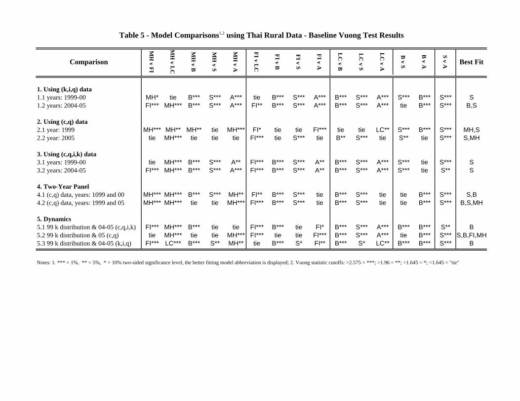
Comparison

MH

v FI

MH

v LC

MH

v B

MH

v S

MH

v A

FI v LC

FI v B

FI v S

FI v A

LC

v B

LC

v S

LC

v A

B v S

B v A

S v A Best Fit

1. Using (k,i,q) data1.1 years: 1999-00 MH* tie B*** S*** A*** tie B*** S*** A*** B*** S*** A*** S*** B*** S*** S1.2 years: 2004-05 FI*** MH*** B*** S*** A*** FI** B*** S*** A*** B*** S*** A*** tie B*** S*** B,S

2. Using (c,q) data2.1 year: 1999 MH*** MH** MH** tie MH*** FI* tie tie FI*** tie tie LC** S*** B*** S*** MH,S2.2 year: 2005 tie MH*** tie tie tie FI*** tie S*** tie B** S*** tie S** tie S*** S,MH

3. Using (c,q,i,k) data3.1 years: 1999-00 tie MH*** B*** S*** A** FI*** B*** S*** A** B*** S*** A*** S*** tie S*** S3.2 years: 2004-05 FI*** MH*** B*** S*** A*** FI*** B*** S*** A** B*** S*** A*** S*** tie S** S

4. Two-Year Panel4.1 (c,q) data, years: 1099 and 00 MH*** MH*** B*** S*** MH** FI** B*** S*** tie B*** S*** tie tie B*** S*** S,B4.2 (c,q) data, years: 1999 and 05 MH*** MH*** tie tie MH*** FI*** B*** S*** tie B*** S*** tie tie B*** S*** B,S,MH

5. Dynamics5.1 99 k distribution & 04-05 (c,q,i,k) FI*** MH*** B*** tie tie FI*** B*** tie FI* B*** S*** A*** B*** B*** S** B5.2 99 k distribution & 05 (c,q) tie MH*** tie tie MH*** FI*** tie tie FI*** B*** S*** A*** tie B*** S*** S,B,FI,MH5.3 99 k distribution & 04-05 (k,i,q) FI*** LC*** B*** S** MH** tie B*** S* FI** B*** S* LC** B*** B*** S*** B

Notes: 1. *** = 1%, ** = 5%, * = 10% two-sided significance level, the better fitting model abbreviation is displayed; 2. Vuong statistic cutoffs: >2.575 = ***; >1.96 = **; >1.645 = *; <1.645 = "tie"

Table 5 - Model Comparisons1,2 using Thai Rural Data - Baseline Vuong Test Results

Karaivanov and Townsend Dynamic Financial Constraints

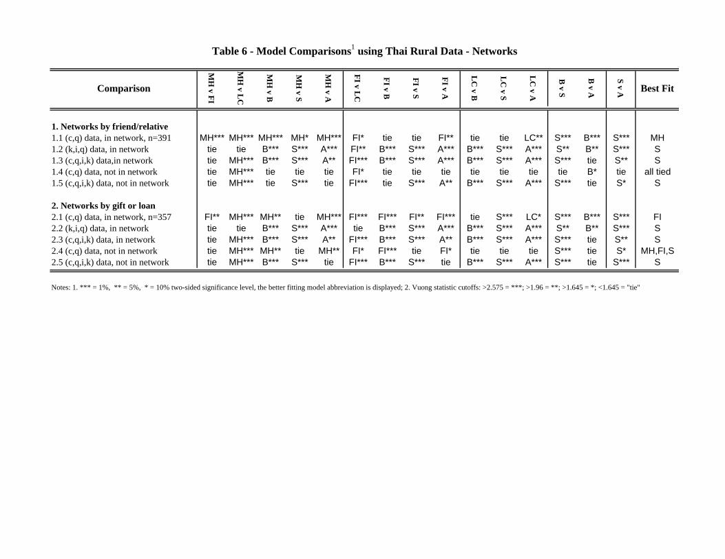
Thai data — results

• Networks (Table 6), by blood/kinship or loan/gift — evidence for moralhazard in c, q data

Toulouse, January 2012 31

Comparison

MH

v FI

MH

v LC

MH

v B

MH

v S

MH

v A

FI v LC

FI v B

FI v S

FI v A

LC

v B

LC

v S

LC

v A

B v S

B v A

S v A Best Fit

1. Networks by friend/relative1.1 (c,q) data, in network, n=391 MH*** MH*** MH*** MH* MH*** FI* tie tie FI** tie tie LC** S*** B*** S*** MH1.2 (k,i,q) data, in network tie tie B*** S*** A*** FI** B*** S*** A*** B*** S*** A*** S** B** S*** S1.3 (c,q,i,k) data,in network tie MH*** B*** S*** A** FI*** B*** S*** A*** B*** S*** A*** S*** tie S** S1.4 (c,q) data, not in network tie MH*** tie tie tie FI* tie tie tie tie tie tie tie B* tie all tied1.5 (c,q,i,k) data, not in network tie MH*** tie S*** tie FI*** tie S*** A** B*** S*** A*** S*** tie S* S

2. Networks by gift or loan2.1 (c,q) data, in network, n=357 FI** MH*** MH** tie MH*** FI*** FI*** FI** FI*** tie S*** LC* S*** B*** S*** FI2.2 (k,i,q) data, in network tie tie B*** S*** A*** tie B*** S*** A*** B*** S*** A*** S** B** S*** S2.3 (c,q,i,k) data, in network tie MH*** B*** S*** A** FI*** B*** S*** A** B*** S*** A*** S*** tie S** S2.4 (c,q) data, not in network tie MH*** MH** tie MH** FI* FI*** tie FI* tie tie tie S*** tie S* MH,FI,S2.5 (c,q,i,k) data, not in network tie MH*** B*** S*** tie FI*** B*** S*** tie B*** S*** A*** S*** tie S*** S

Notes: 1. *** = 1%, ** = 5%, * = 10% two-sided significance level, the better fitting model abbreviation is displayed; 2. Vuong statistic cutoffs: >2.575 = ***; >1.96 = **; >1.645 = *; <1.645 = "tie"

Table 6 - Model Comparisons1 using Thai Rural Data - Networks

Karaivanov and Townsend Dynamic Financial Constraints

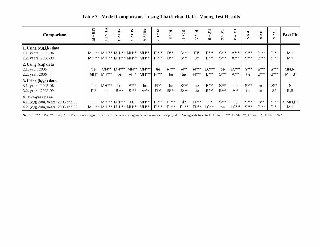
Thai data — results

• Thai urban data (Table 7) — evidence for moral hazard in c, q andc, q, i, k data

Toulouse, January 2012 32

Comparison

MH

v FI

MH

v LC

MH

v B

MH

v S

MH

v A

FI v LC

FI v B

FI v S

FI v A

LC

v B

LC

v S

LC

v A

B v S

B v A

S v A Best Fit

1. Using (c,q,i,k) data1.1. years: 2005-06 MH*** MH*** MH*** MH*** MH*** FI*** B*** S*** FI* B*** S*** A*** S*** B*** S*** MH1.2. years: 2008-09 MH*** MH*** MH*** MH*** MH*** FI*** B*** S*** tie B*** S*** A*** S*** B*** S*** MH2. Using (c,q) data2.1. year: 2005 tie MH** MH*** MH** MH*** tie FI*** FI** FI*** LC*** tie LC*** S*** B*** S*** MH,FI2.2. year: 2009 MH* MH*** tie MH* MH*** FI*** tie tie FI*** B*** S*** A*** tie B*** S*** MH,B3. Using (k,i,q) data3.1. years: 2005-06 tie MH*** tie S*** tie FI** tie S*** tie B*** S*** tie S*** tie S** S3.2. years: 2008-09 FI* tie B*** S*** A*** FI** B*** S*** tie B*** S*** A** tie tie S* S,B4. Two-year panel4.1. (c,q) data, years: 2005 and 06 tie MH*** MH*** tie MH*** FI*** FI*** tie FI*** tie S*** tie S*** B** S*** S,MH,FI4.2. (c,q) data, years: 2005 and 09 MH*** MH*** MH*** MH*** MH*** FI*** FI*** FI*** FI*** LC*** tie LC*** S*** B*** S*** MH

Notes: 1. *** = 1%, ** = 5%, * = 10% two-sided significance level, the better fitting model abbreviation is displayed; 2. Vuong statistic cutoffs: >2.575 = ***; >1.96 = **; >1.645 = *; <1.645 = "tie"

Table 7 - Model Comparisons1,2 using Thai Urban Data - Vuong Test Results

Karaivanov and Townsend Dynamic Financial Constraints

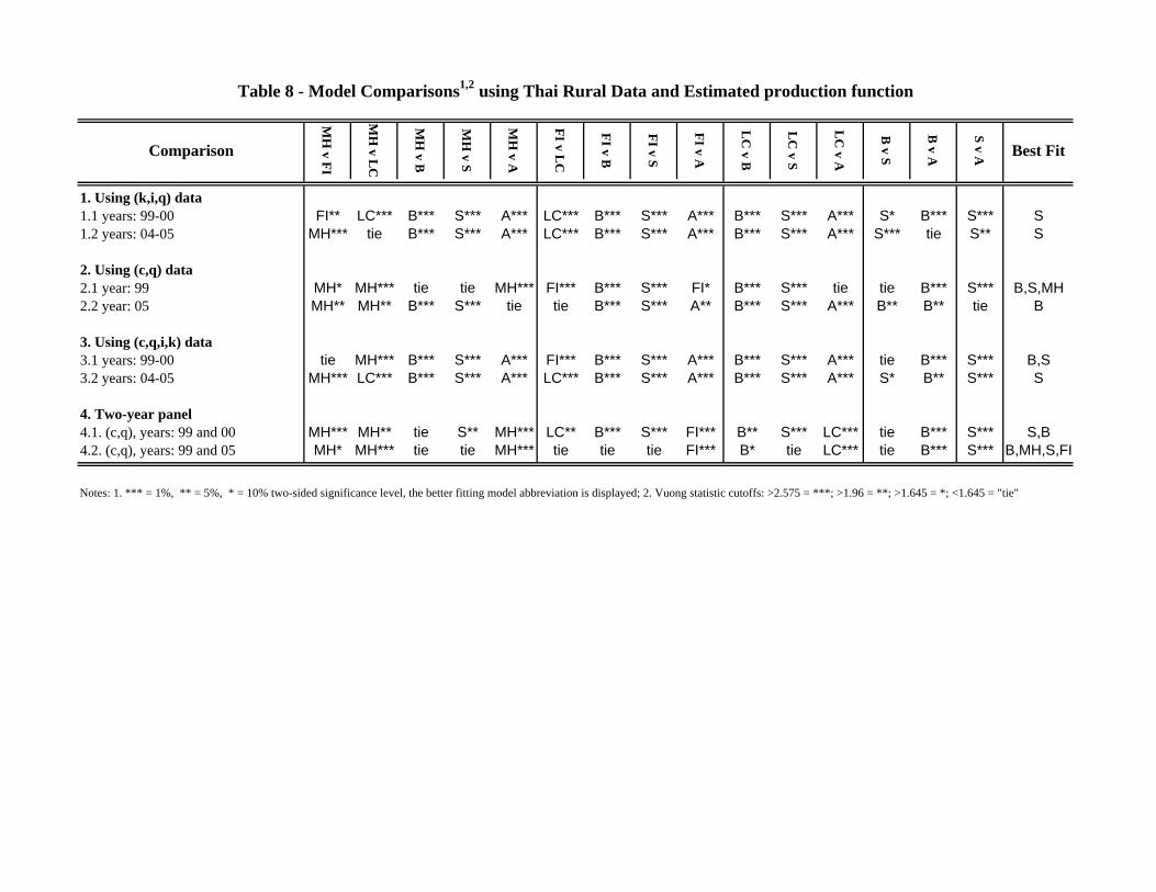
Thai data — robustness

• estimated production function (Table 8)

Toulouse, January 2012 33

Comparison

MH

v FI

MH

v LC

MH

v B

MH

v S

MH

v A

FI v LC

FI v B

FI v S

FI v A

LC

v B

LC

v S

LC

v A

B v S

B v A

S v A Best Fit

1. Using (k,i,q) data1.1 years: 99-00 FI** LC*** B*** S*** A*** LC*** B*** S*** A*** B*** S*** A*** S* B*** S*** S1.2 years: 04-05 MH*** tie B*** S*** A*** LC*** B*** S*** A*** B*** S*** A*** S*** tie S** S

2. Using (c,q) data2.1 year: 99 MH* MH*** tie tie MH*** FI*** B*** S*** FI* B*** S*** tie tie B*** S*** B,S,MH2.2 year: 05 MH** MH** B*** S*** tie tie B*** S*** A** B*** S*** A*** B** B** tie B

3. Using (c,q,i,k) data3.1 years: 99-00 tie MH*** B*** S*** A*** FI*** B*** S*** A*** B*** S*** A*** tie B*** S*** B,S3.2 years: 04-05 MH*** LC*** B*** S*** A*** LC*** B*** S*** A*** B*** S*** A*** S* B** S*** S

4. Two-year panel4.1. (c,q), years: 99 and 00 MH*** MH** tie S** MH*** LC** B*** S*** FI*** B** S*** LC*** tie B*** S*** S,B4.2. (c,q), years: 99 and 05 MH* MH*** tie tie MH*** tie tie tie FI*** B* tie LC*** tie B*** S*** B,MH,S,FI

Notes: 1. *** = 1%, ** = 5%, * = 10% two-sided significance level, the better fitting model abbreviation is displayed; 2. Vuong statistic cutoffs: >2.575 = ***; >1.96 = **; >1.645 = *; <1.645 = "tie"

Table 8 - Model Comparisons1,2 using Thai Rural Data and Estimated production function

Karaivanov and Townsend Dynamic Financial Constraints

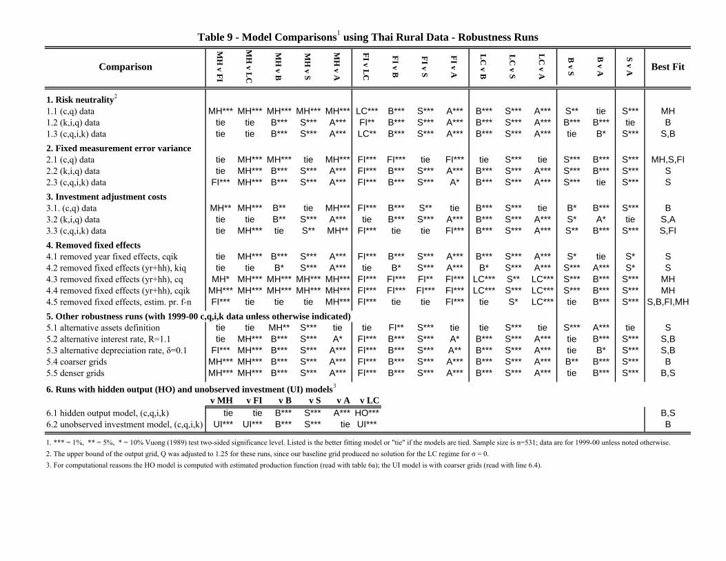
Thai data — robustness

• More robustness checks (Table 9)

• risk neutrality

• fixed measurement error variance

• allowing quadratic adjustment costs in investment

• different grids and samples (alternative definitions of assets; region,household and time fixed effects removed)

• hidden output and unobserved investment regimes

Toulouse, January 2012 34

Comparison

MH

v FI

MH

v LC

MH

v B

MH

v S

MH

v A

FI v LC

FI v B

FI v S

FI v A

LC

v B

LC

v S

LC

v A

B v S

B v A

S v A Best Fit

1. Risk neutrality2

1.1 (c,q) data MH*** MH*** MH*** MH*** MH*** LC*** B*** S*** A*** B*** S*** A*** S** tie S*** MH1.2 (k,i,q) data tie tie B*** S*** A*** FI** B*** S*** A*** B*** S*** A*** B*** B*** tie B1.3 (c,q,i,k) data tie tie B*** S*** A*** LC** B*** S*** A*** B*** S*** A*** tie B* S*** S,B2. Fixed measurement error variance2.1 (c,q) data tie MH*** MH*** tie MH*** FI*** FI*** tie FI*** tie S*** tie S*** B*** S*** MH,S,FI2.2 (k,i,q) data tie MH*** B*** S*** A*** FI*** B*** S*** A*** B*** S*** A*** S*** B*** S*** S2.3 (c,q,i,k) data FI*** MH*** B*** S*** A*** FI*** B*** S*** A* B*** S*** A*** S*** tie S*** S3. Investment adjustment costs3.1. (c,q) data MH** MH*** B** tie MH*** FI*** B*** S** tie B*** S*** tie B* B*** S*** B3.2 (k,i,q) data tie tie B** S*** A*** tie B*** S*** A*** B*** S*** A*** S* A* tie S,A3.3 (c,q,i,k) data tie MH*** tie S** MH** FI*** tie tie FI*** B*** S*** A*** S** B*** S*** S,FI4. Removed fixed effects4.1 removed year fixed effects, cqik tie MH*** B*** S*** A*** FI*** B*** S*** A*** B*** S*** A*** S* tie S* S4.2 removed fixed effects (yr+hh), kiq tie tie B* S*** A*** tie B* S*** A*** B* S*** A*** S*** A*** S* S4.3 removed fixed effects (yr+hh), cq MH* MH*** MH*** MH*** MH*** FI*** FI*** FI** FI*** LC*** S** LC*** S*** B*** S*** MH4.4 removed fixed effects (yr+hh), cqik MH*** MH*** MH*** MH*** MH*** FI*** FI*** FI*** FI*** LC*** S*** LC*** S*** B*** S*** MH4.5 removed fixed effects, estim. pr. f-n FI*** tie tie tie MH*** FI*** tie tie FI*** tie S* LC*** tie B*** S*** S,B,FI,MH5. Other robustness runs (with 1999-00 c,q,i,k data unless otherwise indicated)5.1 alternative assets definition tie tie MH** S*** tie tie FI** S*** tie tie S*** tie S*** A*** tie S5.2 alternative interest rate, R=1.1 tie MH*** B*** S*** A* FI*** B*** S*** A* B*** S*** A*** tie B*** S*** S,B5.3 alternative depreciation rate, δ=0.1 FI*** MH*** B*** S*** A*** FI*** B*** S*** A** B*** S*** A*** tie B* S*** S,B5.4 coarser grids MH*** MH*** B*** S*** A*** FI*** B*** S*** A*** B*** S*** A*** B** B*** S*** B5.5 denser grids MH*** MH*** B*** S*** A*** FI*** B*** S*** A*** B*** S*** A*** tie B*** S*** B,S

6. Runs with hidden output (HO) and unobserved investment (UI) models3

v MH v FI v B v S v A v LC6.1 hidden output model, (c,q,i,k) tie tie B*** S*** A*** HO*** B,S6.2 unobserved investment model, (c,q,i,k) UI*** UI*** B*** S*** tie UI*** B

1. *** = 1%, ** = 5%, * = 10% Vuong (1989) test two-sided significance level. Listed is the better fitting model or "tie" if the models are tied. Sample size is n=531; data are for 1999-00 unless noted otherwise.2. The upper bound of the output grid, Q was adjusted to 1.25 for these runs, since our baseline grid produced no solution for the LC regime for σ = 0.3. For computational reasons the HO model is computed with estimated production function (read with table 6a); the UI model is with coarser grids (read with line 6.4).

Table 9 - Model Comparisons1 using Thai Rural Data - Robustness Runs

Karaivanov and Townsend Dynamic Financial Constraints

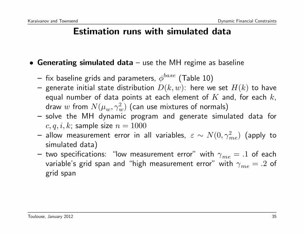
Estimation runs with simulated data

• Generating simulated data — use the MH regime as baseline

— fix baseline grids and parameters, φbase (Table 10)— generate initial state distribution D(k,w): here we set H(k) to haveequal number of data points at each element of K and, for each k,draw w from N(μw, γ

2w) (can use mixtures of normals)

— solve the MH dynamic program and generate simulated data forc, q, i, k; sample size n = 1000

— allow measurement error in all variables, ε ∼ N(0, γ2me) (apply tosimulated data)

— two specifications: “low measurement error” with γme = .1 of eachvariable’s grid span and “high measurement error” with γme = .2 ofgrid span

Toulouse, January 2012 35

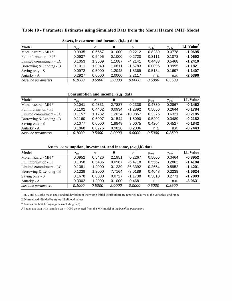
Model γme σ θ ρ μw/b1 γw/b LL Value2

Moral hazard - MH * 0.0935 0.6557 0.1000 0.2212 0.8289 0.0778 -1.0695Full information - FI * 0.0937 0.5495 0.1000 0.2720 0.8111 0.1078 -1.0692Limited commitment - LC 0.1053 1.3509 1.1087 -4.2141 0.4483 0.5468 -1.2410Borrowing & Lending - B 0.1011 1.0940 1.0811 -1.5783 0.0096 0.9995 -1.1821Saving only - S 0.0972 0.5000 1.2043 -1.8369 0.5184 0.1697 -1.1407Autarky - A 0.2927 0.0000 2.0000 2.2117 n.a. n.a. -2.5390baseline parameters 0.1000 0.5000 2.0000 0.0000 0.5000 0.3500

Model γme σ θ ρ μw/b γw/b LL ValueMoral hazard - MH * 0.1041 0.4851 2.7887 -0.2338 0.4780 0.2867 -0.1462Full information - FI 0.1102 0.4462 0.0934 -1.2892 0.5056 0.2644 -0.1784Limited commitment - LC 0.1157 1.1782 1.2024 -10.9857 0.2276 0.6321 -0.2185Borrowing & Lending - B 0.1160 0.6007 0.1544 -1.5090 0.5202 0.3489 -0.2182Saving only - S 0.1077 0.0000 1.9849 3.0075 0.4204 0.4527 -0.1842Autarky - A 0.1868 0.0276 0.9828 0.2036 n.a. n.a. -0.7443baseline parameters 0.1000 0.5000 2.0000 0.0000 0.5000 0.3500

Model γme σ θ ρ μw/b γw/b LL ValueMoral hazard - MH * 0.0952 0.5426 2.1951 0.2267 0.5005 0.3464 -0.8952Full information - FI 0.1358 0.5436 0.0967 -6.4718 0.5567 0.2862 -1.4184Limited commitment - LC 0.1381 1.2000 0.1239 -36.3392 0.2654 0.5952 -1.4201Borrowing & Lending - B 0.1339 1.2000 7.7164 -3.0189 0.4048 0.3238 -1.5624Saving only - S 0.1678 0.0000 0.0727 -1.1738 0.3818 0.2771 -1.7803Autarky - A 0.3302 1.2000 0.1000 0.4681 n.a. n.a. -3.0631baseline parameters 0.1000 0.5000 2.0000 0.0000 0.5000 0.3500

1. μw/b and γw/b (the mean and standard deviation of the w or b initial distribution) are reported relative to the variables' grid range2. Normalized (divided by n) log-likelihood values; * denotes the best fitting regime (including tied)All runs use data with sample size n=1000 generated from the MH model at the baseline parameters

Assets, investment and income, (k,i,q) data

Consumption and income, (c,q) data

Assets, consumption, investment, and income, (c,q,i,k) data

Table 10 - Parameter Estimates using Simulated Data from the Moral Hazard (MH) Model

Comparison

MH

v FI

MH

v LC

MH

v B

MH

v S

MH

v A

FI v LC

FI v B

FI v S

FI v A

LC

v B

LC

v S

LC

v A

B v S

B v A

S v A Best Fit

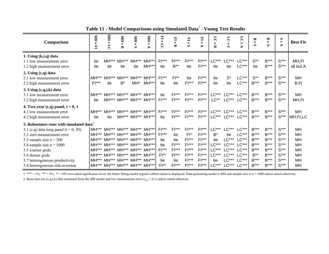
1. Using (k,i,q) data1.1 low measurement error tie MH*** MH*** MH*** MH*** FI*** FI*** FI*** FI*** LC*** LC*** LC*** S** B*** S*** MH,FI1.2 high measurement error tie tie tie tie MH*** tie B** tie FI*** tie tie LC*** tie B*** S*** all but A2. Using (c,q) data2.1 low measurement error MH*** MH*** MH*** MH*** MH*** FI*** FI** tie FI*** tie S* LC*** S** B*** S*** MH2.2 high measurement error FI*** tie B* MH* MH*** tie tie FI*** FI*** tie tie LC*** B*** B*** S*** B,FI3. Using (c,q,i,k) data3.1 low measurement error MH*** MH*** MH*** MH*** MH*** tie FI*** FI*** FI*** LC*** LC*** LC*** B*** B*** S*** MH3.2 high measurement error tie MH*** MH*** MH*** MH*** FI*** FI*** FI*** FI*** LC** LC*** LC*** B*** B*** S*** MH,FI4. Two-year (c,q) panel, t = 0, 14.1 low measurement error MH*** MH*** MH*** MH*** MH*** FI*** FI*** FI*** FI*** LC*** LC*** LC*** B*** B*** S*** MH4.2 high measurement error tie tie MH*** MH*** MH*** tie FI*** FI*** FI*** LC*** LC*** LC*** B*** B*** S*** MH,FI,LC

5. Robustness runs with simulated data2

5.1 (c,q) data long panel (t = 0, 50) MH*** MH*** MH*** MH*** MH*** FI*** FI*** FI*** FI*** LC*** LC*** LC*** B*** B*** S*** MH5.2 zero measurement error MH*** MH*** MH*** MH*** MH*** FI*** tie FI* FI*** B* tie LC*** B*** B*** S*** MH5.3 sample size n = 200 MH*** MH*** MH*** MH*** MH*** tie tie FI*** FI*** tie LC*** LC*** B*** B*** S*** MH5.4 sample size n = 5000 MH*** MH*** MH*** MH*** MH*** tie FI*** FI*** FI*** LC*** LC*** LC*** B*** B*** S*** MH5.5 coarser grids MH*** MH*** MH*** MH*** MH*** FI*** FI*** FI*** FI*** LC*** LC*** LC*** B*** B*** S*** MH5.6 denser grids MH*** MH*** MH*** MH*** MH*** FI** FI*** FI*** FI*** LC*** LC*** LC*** B** B*** S*** MH5.7 heterogeneous productivity MH*** MH*** MH*** MH*** MH*** tie tie FI*** FI*** tie LC*** LC*** B*** B*** S*** MH5.8 heterogeneous risk-aversion MH*** MH*** MH*** MH*** MH*** FI** FI*** FI*** FI*** LC*** LC*** LC*** B*** B*** S*** MH

1. *** = 1%, ** = 5%, * = 10% two-sided significance level, the better fitting model regime's abbreviation is displayed. Data-generating model is MH and sample size is n = 1000 unless stated otherwise.2. these runs use (c,q,i,k) data simulated from the MH model and low measurement error (γme = 0.1) unless stated otherwise

Table 11 - Model Comparisons using Simulated Data1 - Vuong Test Results

Karaivanov and Townsend Dynamic Financial Constraints

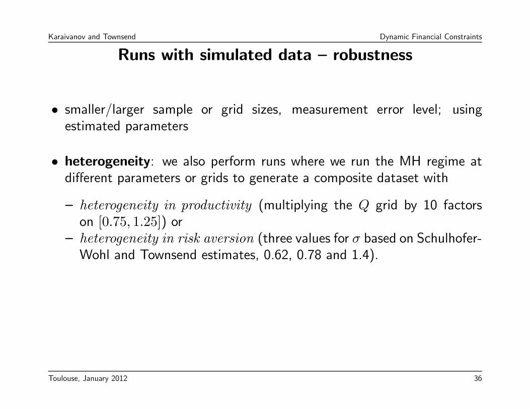
Runs with simulated data — robustness

• smaller/larger sample or grid sizes, measurement error level; usingestimated parameters

• heterogeneity: we also perform runs where we run the MH regime atdifferent parameters or grids to generate a composite dataset with

— heterogeneity in productivity (multiplying the Q grid by 10 factorson [0.75, 1.25]) or

— heterogeneity in risk aversion (three values for σ based on Schulhofer-Wohl and Townsend estimates, 0.62, 0.78 and 1.4).

Toulouse, January 2012 36

Karaivanov and Townsend Dynamic Financial Constraints

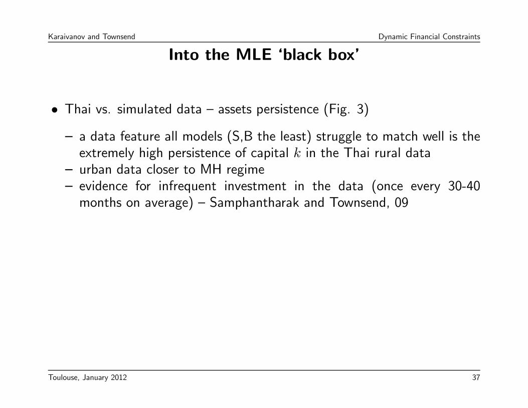
Into the MLE ‘black box’

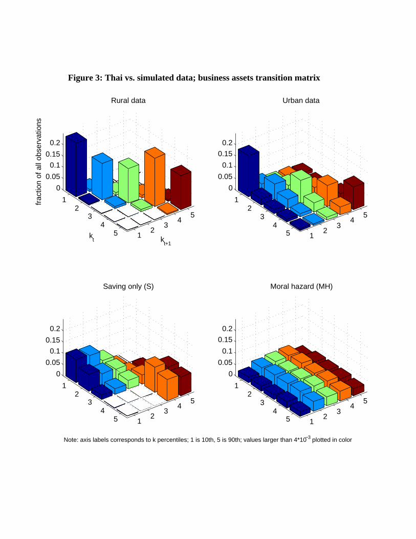
• Thai vs. simulated data — assets persistence (Fig. 3)

— a data feature all models (S,B the least) struggle to match well is theextremely high persistence of capital k in the Thai rural data

— urban data closer to MH regime— evidence for infrequent investment in the data (once every 30-40months on average) — Samphantharak and Townsend, 09

Toulouse, January 2012 37

12

34

5

12

34

5

0

0.05

0.1

0.15

0.2

Urban data

12

34

5

12

34

5

0

0.05

0.1

0.15

0.2

Moral hazard (MH)

12

34

5

12

34

5

0

0.05

0.1

0.15

0.2

kt+1

Rural data

kt

frac

tion

of a

ll ob

serv

atio

ns

12

34

5

12

34

5

0

0.05

0.1

0.15

0.2

Saving only (S)

Figure 3: Thai vs. simulated data; business assets transition matrix

Note: axis labels corresponds to k percentiles; 1 is 10th, 5 is 90th; values larger than 4*10−3 plotted in color

Karaivanov and Townsend Dynamic Financial Constraints

Into the MLE ‘black box’

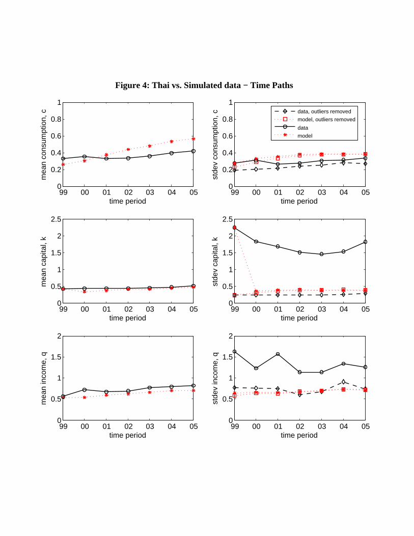
• Thai vs. simulated data — time paths (Fig. 4)

Toulouse, January 2012 38

99 00 01 02 03 04 050

0.2

0.4

0.6

0.8

1

mea

n co

nsum

ptio

n, c

time period99 00 01 02 03 04 05

0

0.2

0.4

0.6

0.8

1

stde

v co

nsum

ptio

n, c

time period

99 00 01 02 03 04 050

0.5

1

1.5

2

2.5

mea

n ca

pita

l, k

time period99 00 01 02 03 04 05

0

0.5

1

1.5

2

2.5st

dev

capi

tal,

k

time period

99 00 01 02 03 04 050

0.5

1

1.5

2

mea

n in

com

e, q

time period99 00 01 02 03 04 05

0

0.5

1

1.5

2

stde

v in

com

e, q

time period

data, outliers removed

model, outliers removed

data

model

Figure 4: Thai vs. Simulated data − Time Paths

Karaivanov and Townsend Dynamic Financial Constraints

Into the MLE ‘black box’

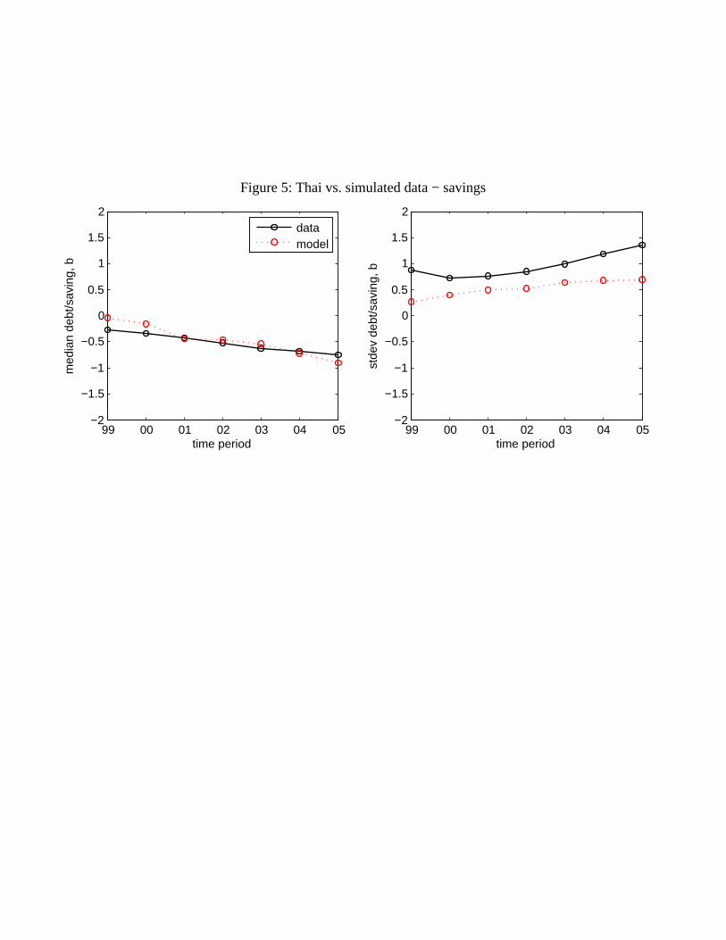
• Thai vs. simulated data — financial net worth (Fig. 5)

Toulouse, January 2012 39

99 00 01 02 03 04 05−2

−1.5

−1

−0.5

0

0.5

1

1.5

2

med

ian

debt

/sav

ing,

b

time period

datamodel

99 00 01 02 03 04 05−2

−1.5

−1

−0.5

0

0.5

1

1.5

2

stde

v de

bt/s

avin

g, b

time period

Figure 5: Thai vs. simulated data − savings

Karaivanov and Townsend Dynamic Financial Constraints

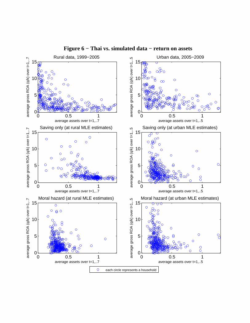
Into the MLE ‘black box’

• Thai vs. simulated data — ROA (Fig. 6)

Toulouse, January 2012 40

0 0.5 10

5

10

15

average assets over t=1,..5

aver

age

gros

s R

OA

(q/

k) o

ver

t=1,

..5

Urban data, 2005−2009

0 0.5 10

5

10

15

average assets over t=1,..5

aver

age

gros

s R

OA

(q/

k) o

ver

t=1,

..5Saving only (at urban MLE estimates)

0 0.5 10

5

10

15

average assets over t=1,..5

aver

age

gros

s R

OA

(q/

k) o

ver

t=1,

..5

Moral hazard (at urban MLE estimates)

0 0.5 10

5

10

15

average assets over t=1,..7

aver

age

gros

s R

OA

(q/

k) o

ver

t=1,

..7

Rural data, 1999−2005

0 0.5 10

5

10

15

average assets over t=1,..7

aver

age

gros

s R

OA

(q/

k) o

ver

t=1,

..7

Saving only (at rural MLE estimates)

0 0.5 10

5

10

15

average assets over t=1,..7

aver

age

gros

s R

OA

(q/

k) o

ver

t=1,

..7

Moral hazard (at rural MLE estimates)

each circle represents a household

Figure 6 − Thai vs. simulated data − return on assets

Karaivanov and Townsend Dynamic Financial Constraints

Into the MLE ‘black box’

• alternative measure of fit, Dm =P#s

j=1

(sdataj −smj )2

|sdataJ

| where sj denote

various moments of c, q, i, k (mean, median, stdev, skewness,correlations)

model, m = MH FI B S A LCcriterion value (rural), Dm = 321.1 395.4 38.5 20.8 28.1 6520criterion value (urban), Dm = 36.8 32.0 36.4 35.3 35.4 236.7

Toulouse, January 2012 41

Karaivanov and Townsend Dynamic Financial Constraints

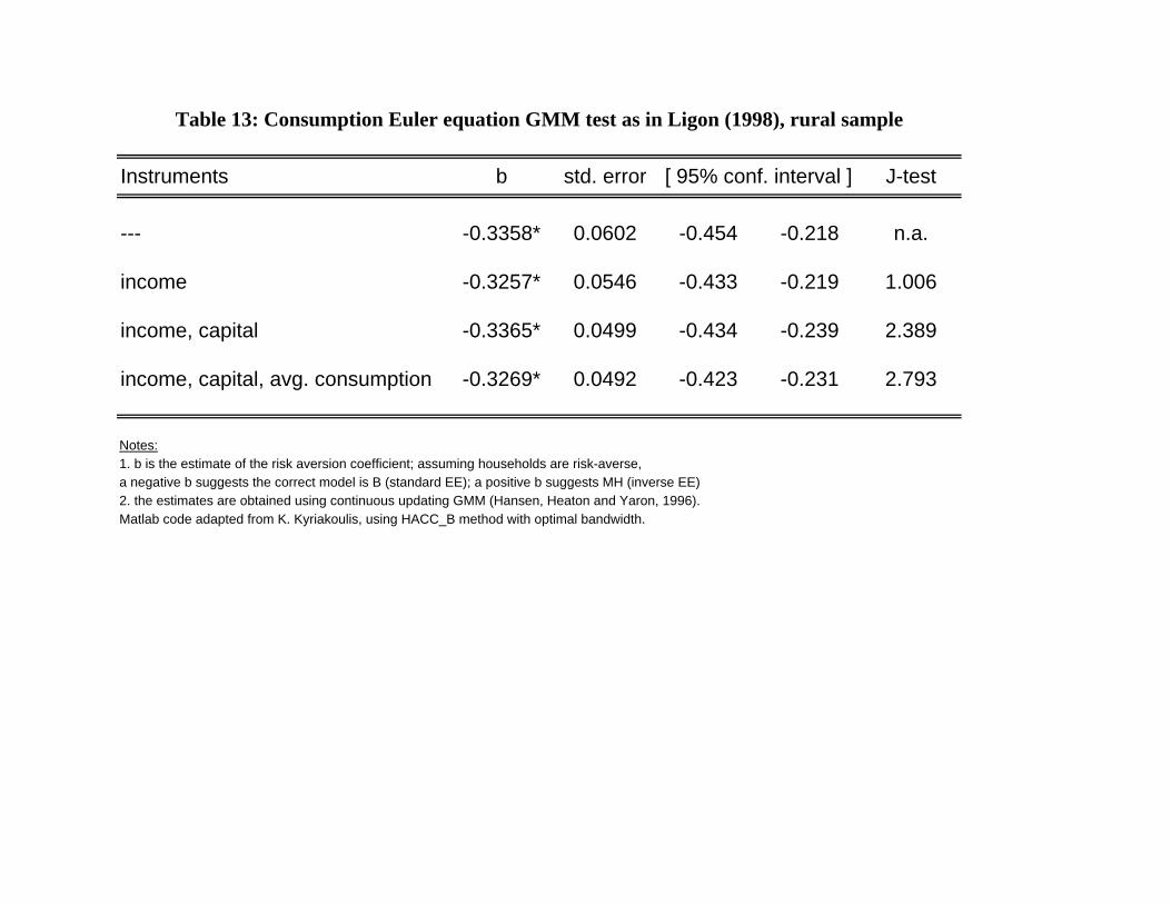
Thai data — GMM robustness checks — consumption

• Based on Ligon (1998), run a consumption-based Euler equation GMMestimation (*this method uses c time-series data alone) to test:

— the ‘standard EE’, u0(ct) = βREu0(ct+1) in the B model vs.

— the ‘inverse EE’, 1u0(ct)

= 1βRE(

1u0(ct+1)

) in the MH model

— assuming CRRA utility the sign of the GMM estimate of parameterb (= −σ or σ depending on regime) in the moment equationEt(h(ξ

bit, b)) = 0 where ξit =

ci,t+1citis used to distinguish B vs. MH

— additional pre-determined variables (income, capital, averageconsumption) can be used as instruments

• Result: further evidence favoring the exogenously incomplete regimes inthe Thai rural data.

Toulouse, January 2012 42

Instruments b std. error J-test

--- -0.3358* 0.0602 -0.454 -0.218 n.a.

income -0.3257* 0.0546 -0.433 -0.219 1.006

income, capital -0.3365* 0.0499 -0.434 -0.239 2.389

income, capital, avg. consumption -0.3269* 0.0492 -0.423 -0.231 2.793

Notes:1. b is the estimate of the risk aversion coefficient; assuming households are risk-averse, a negative b suggests the correct model is B (standard EE); a positive b suggests MH (inverse EE)2. the estimates are obtained using continuous updating GMM (Hansen, Heaton and Yaron, 1996). Matlab code adapted from K. Kyriakoulis, using HACC_B method with optimal bandwidth.

Table 13: Consumption Euler equation GMM test as in Ligon (1998), rural sample

[ 95% conf. interval ]

Karaivanov and Townsend Dynamic Financial Constraints

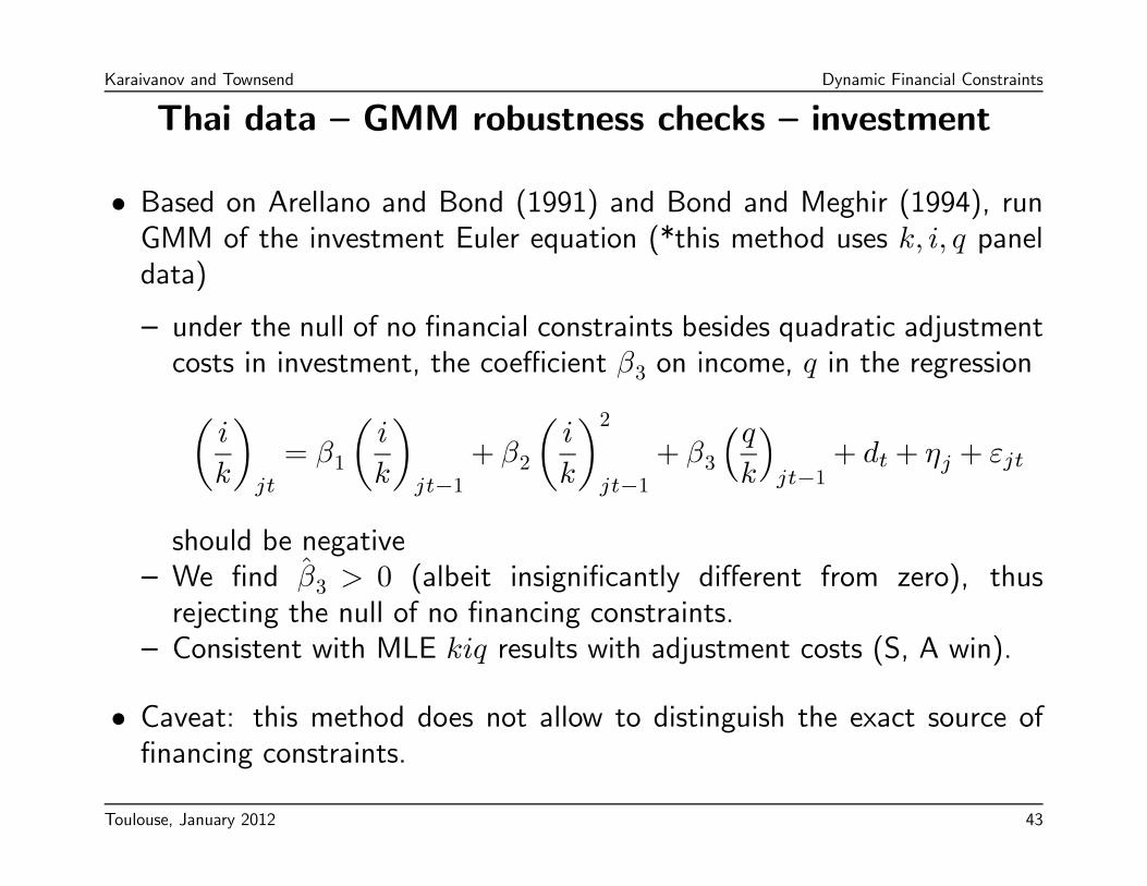
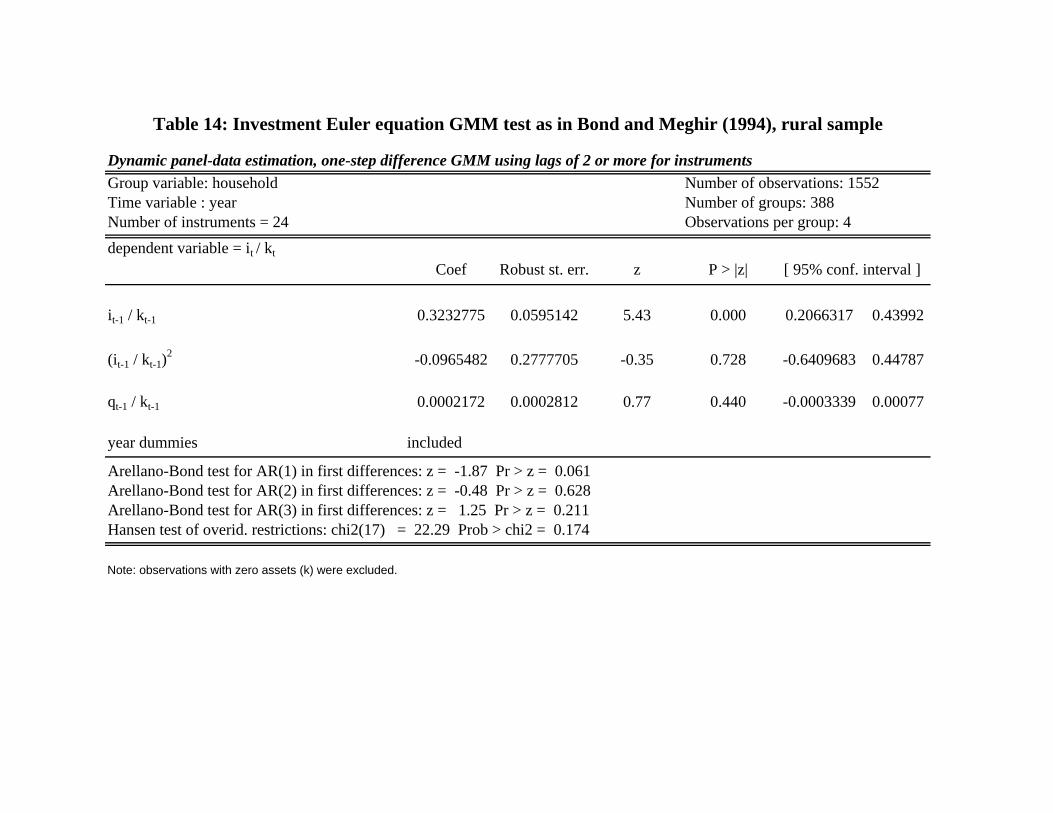
Thai data — GMM robustness checks — investment

• Based on Arellano and Bond (1991) and Bond and Meghir (1994), runGMM of the investment Euler equation (*this method uses k, i, q paneldata)

— under the null of no financial constraints besides quadratic adjustmentcosts in investment, the coefficient β3 on income, q in the regressionµ

i

k

¶jt

= β1

µi

k

¶jt−1

+ β2

µi

k

¶2jt−1

+ β3

³qk

´jt−1

+ dt + ηj + εjt

should be negative— We find β3 > 0 (albeit insignificantly different from zero), thusrejecting the null of no financing constraints.

— Consistent with MLE kiq results with adjustment costs (S, A win).

• Caveat: this method does not allow to distinguish the exact source offinancing constraints.

Toulouse, January 2012 43

Dynamic panel-data estimation, one-step difference GMM using lags of 2 or more for instrumentsGroup variable: household Number of observations: 1552Time variable : year Number of groups: 388Number of instruments = 24 Observations per group: 4dependent variable = it / kt

Coef Robust st. err. z P > |z|

it-1 / kt-1 0.3232775 0.0595142 5.43 0.000 0.2066317 0.43992

(it-1 / kt-1)2 -0.0965482 0.2777705 -0.35 0.728 -0.6409683 0.44787

qt-1 / kt-1 0.0002172 0.0002812 0.77 0.440 -0.0003339 0.00077

year dummies included

Arellano-Bond test for AR(1) in first differences: z = -1.87 Pr > z = 0.061Arellano-Bond test for AR(2) in first differences: z = -0.48 Pr > z = 0.628Arellano-Bond test for AR(3) in first differences: z = 1.25 Pr > z = 0.211Hansen test of overid. restrictions: chi2(17) = 22.29 Prob > chi2 = 0.174

Note: observations with zero assets (k) were excluded.

Table 14: Investment Euler equation GMM test as in Bond and Meghir (1994), rural sample

[ 95% conf. interval ]

Karaivanov and Townsend Dynamic Financial Constraints

Future work

• further work on the theory given our findings with the Thai data

— multiple technologies, aggregate shocks, entrepreneurial ability, explicitadjustment costs

— other regimes — costly state verification, limited enforcement— transitions between regimes

• data from other economies, e.g. Spain — more entry-exit, larger samplesize (joint work with Ruano and Saurina)

• supply side — lenders’ rules for access, regulatory distortions (Assuncao,Mityakov and Townsend, 09)

• computational methods — parallel processing; MPEC (Judd and Su, 09);NPL (Aguiregabirria and Mira; Kasahara and Shimotsu)

Toulouse, January 2012 44

Karaivanov and Townsend Dynamic Financial Constraints

Technology

• technology (if functional form used): for q ∈ qmin, ..., q#Q ≡ Q

Prob(q = qmin) = 1− (kρ + zρ

2)1/ρ

Prob(q = qi, i 6= min) =1

#Q− 1(kρ + zρ

2)1/ρ

ρ = 0 is perfect substitutes; ρ→ −∞ is Leontieff; ρ→ 0 is Cobb-Douglas

Toulouse, January 2012 45

Karaivanov and Townsend Dynamic Financial Constraints

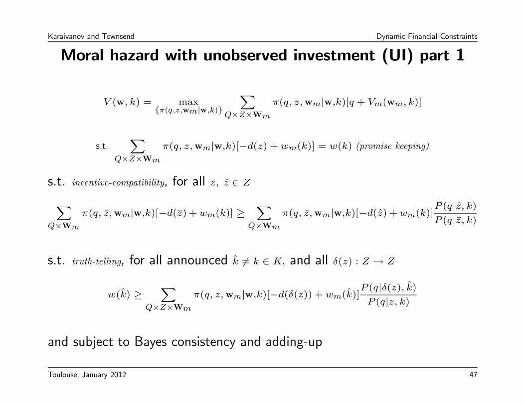
Moral hazard with unobserved investment (UI)

• Structure

— unobserved: effort z; capital stock / investment k, i— observed: output q— dynamic moral hazard and adverse selection: both incentive andtruth-telling constraints

— the feasible promise functions set W is endogenously determined anditerated on together with V (Abreu, Pierce and Stacchetti, 1990)

• LP formulation

— state variables: k ∈ K and a vector of promises,w ≡ w(k1), w(k2), ...w(k#K) ∈W (Fernandes and Phelan, 2000)

— assume separable utility, U(c, z) = u(c) − d(z) to divide theoptimization problem into two sub-periods and reduce dimensionality;wm — vector of interim promised utilities

Toulouse, January 2012 46

Karaivanov and Townsend Dynamic Financial Constraints

Moral hazard with unobserved investment (UI) part 1

V (w, k) = maxπ(q,z,wm|w,k)Q×Z×Wm

π(q, z,wm|w,k)[q + Vm(wm, k)]

s.t.

Q×Z×Wm

π(q, z,wm|w,k)[−d(z) + wm(k)] = w(k) (promise keeping)

s.t. incentive-compatibility, for all z, z ∈ Z

Q×Wm

π(q, z,wm|w,k)[−d(z) +wm(k)] ≥Q×Wm

π(q, z,wm|w,k)[−d(z) +wm(k)]P (q|z, k)P (q|z, k)

s.t. truth-telling, for all announced k 6= k ∈ K, and all δ(z) : Z → Z

w(k) ≥Q×Z×Wm

π(q, z,wm|w,k)[−d(δ(z)) + wm(k)]P (q|δ(z), k)P (q|z, k)

and subject to Bayes consistency and adding-up

Toulouse, January 2012 47

Karaivanov and Townsend Dynamic Financial Constraints

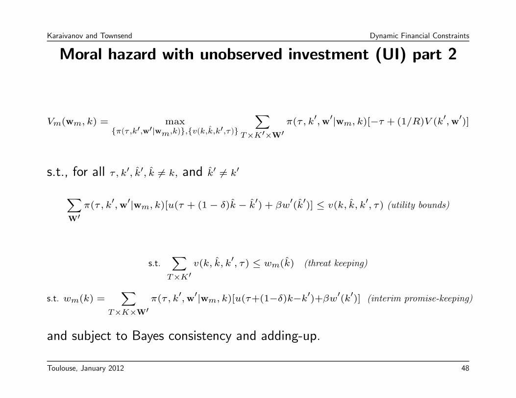
Moral hazard with unobserved investment (UI) part 2

Vm(wm, k) = maxπ(τ,k0,w0|wm,k),v(k,k,k0,τ)

T×K0×W0π(τ, k0,w0|wm, k)[−τ + (1/R)V (k0,w0)]

s.t., for all τ, k0, k0, k 6= k, and k0 6= k0

W0π(τ, k0,w0|wm, k)[u(τ + (1− δ)k − k0) + βw0(k0)] ≤ v(k, k, k0, τ) (utility bounds)

s.t.

T×K0v(k, k, k0, τ) ≤ wm(k) (threat keeping)

s.t. wm(k) =

T×K×W0π(τ, k0,w0|wm, k)[u(τ+(1−δ)k−k0)+βw0(k0)] (interim promise-keeping)

and subject to Bayes consistency and adding-up.

Toulouse, January 2012 48