Dynamic Analysis

With Emphasis On

Wind and Earthquake LoadsBY

Ed WilsonProfessor Emeritus of Structural Engineering

University of California, Berkeley

October 22, 1999

Summary Of Presentation1. General Comments

2. History Of The Development of SAP 3. Computer Hardware Developments

4. Methods For Linear and Nonlinear Analysis

5. Generation And Use Of LDR Vectors and Fast Nonlinear Analysis - FNA Method

6. Example Of Parallel EngineeringAnalysis of the Richmond - San Rafael Bridge

Structural Engineering IsThe Art Of Using MaterialsWhich We Do Not Fully Understand

To Build Structural SystemsWhich Can Only Be Approximately Analyzed

To Withstand ForcesWhich Are Not Accurately Known

So That We Can SatisfyOur Responsibilities

In Regards To Public Safety

FUNDAMENTALS OF ANALYSIS

1. UNDERSTAND PHYSICS OF PROBLEM

2. CREATE COMPUTER MODEL

3. CONDUCT PARAMETER STUDIES

4. VERIFICATION OF RESULTS STATIC AND DYNAMIC EQUILIBRIUM ENERGY BALANCE

5. FIELD OR LABORATORY TESTS

FIELD MEASUREMENTSREQUIRED TO VERIFY

1. MODELING ASSUMPTIONS

2. SOIL-STRUCTURE MODEL

3. COMPUTER PROGRAM

4. COMPUTER USER

MECHANICALVIBRATIONDEVICES

CHECK OF RIGIDDIAPHRAGMAPPROXIMATION

FIELD MEASUREMENTS OFPERIODS AND MODE SHAPESMODE TFIELD TANALYSIS Diff. - %

1 1.77 Sec. 1.78 Sec. 0.5

2 1.69 1.68 0.6

3 1.68 1.68 0.0

4 0.60 0.61 0.9

5 0.60 0.61 0.9

6 0.59 0.59 0.8

7 0.32 0.32 0.2

- - - -

11 0.23 0.32 2.3

15 th Period

TFIELD = 0.16 Sec.

FIRST DIAPHRAGMMODE SHAPE

COMPUTERS

1957 TO 1999

IBM 701 - PENTIUM III

1957 1999C = Cost of $1,000,000 $1,000 ComputerS = Monthly Salary $1000 $10,000 EngineerC/S RATIO 1,000 .1

1957 1999Time

A Factor Of 10,000Reduction In 42 Years

$

Floating Point Speed Comparison

Year COMPUTER Op/Sec Relative Speed

1981 CRAY-XMP 30,000,000 600

Definition of one Operation A = B + C*D

1997 Pentium Pro 10,000,000 2001998 Pentium II 17,000,000 3501999 Pentium III 45,000,000 900

FORTRAN 64 bits - REAL*8

1963 CDC-6400 50,000 1

1967 CDC-6600 200,000 4

1974 CRAY - 1 3,000,000 60

1988 Intel 80387 100,000 2

1980 VAX - 780 100,000- 2-

1990 DEC-5000 3,500,000 70 1994 Pentium 90 3,500,000 70

1995 DEC - ? 14,500,000 280

Floating Point Speed Comparison - PC

Year CPU Speed MHz Op/Sec Normalized

1980 8080 4 200 1

Definition of one Operation A = B + C*D

1984 8087 10 13,000 65

1988 80387 20 93,000 465

1991 80486 33 605,000 3,O25

1994 PENTIUM 66 1,210,000 6,050

1996 Pentium-Pro 200 10,000,000 50,000

Microsoft FORTRAN 64 bits - REAL*8

1996 PENTIUM 133 5,200,000 26,000

1998 Pentium II 333 17,000,000 85,0001999 Pentium III 450 45,000,000 225,000

The Sap Series

Structural Analysis Programs

1969 To 1999

S A P

STRUCTURAL ANALYSIS

PROGRAM

ALSO A PERSON

“ Who Is Easily Deceived Or Fooled”

“ Who Unquestioningly Serves Another”

"The slang name S A P wasselected to remind the user that

this program, like all programs, lacksintelligence.

It is the responsibility of theengineer to idealize the structure

correctly and assume responsibilityfor the results.”

Ed Wilson 1970

From The Foreword Of The First SAP Manual

The Sap Series Of Programs1969 SAP With User Defined Ritz Vectors

1971 SOLID SAP For Static Loads Only

1972 SAP IV With Full Dynamic Response

1973 NONSAP Now ADINA

1980 SAP 80 NEW Program for PC , Elements and Methods

1983 SAP 80 CSI Added Pre and Design Post Processing

1989 SAP 90 Large Capacity on PC

1991 SADSAP R & D Program With Nonlinear Elements

1997 SAP 2000 Added Graphical User Interface

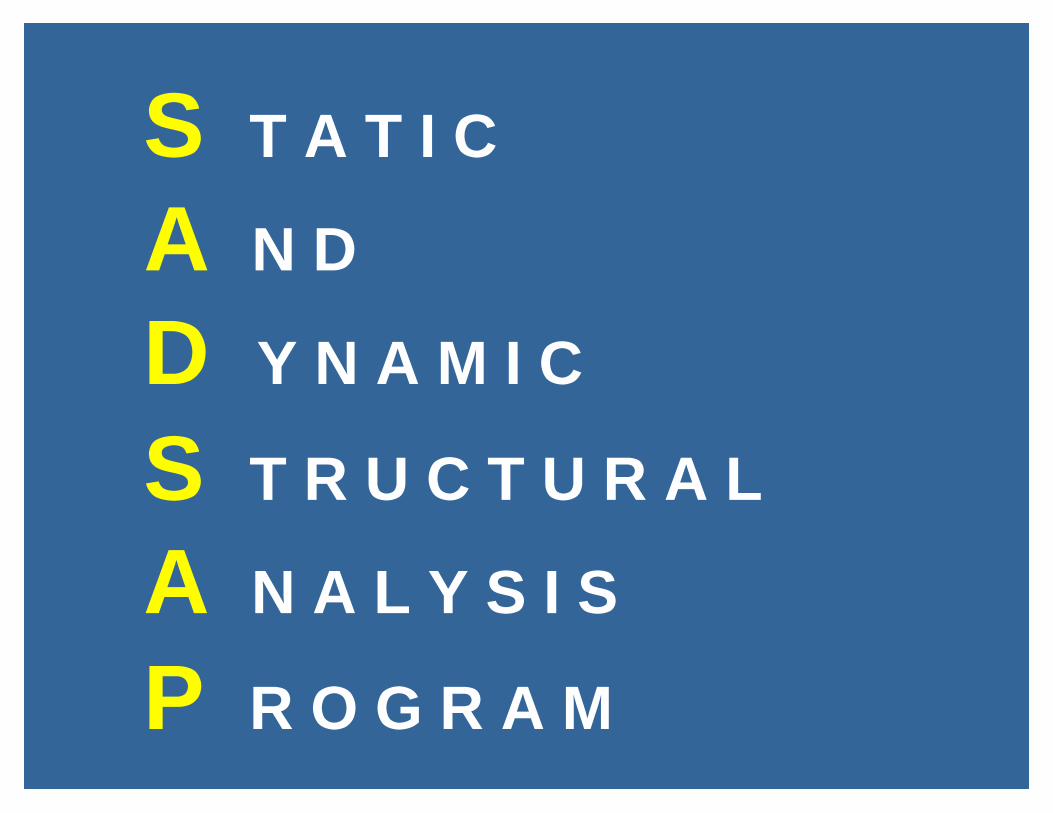
S T A T I C

A N D

D Y N A M I C

S T R U C T U R A L

A N A L Y S I S

P R O G R A M

How Can Engineers BeConvinced To Use New And

Improved Methods Of Analysis ?1. Give Them New Capabilities Such As 2 and 3d Nonlinear Analyses

2. Or, The Program Must Be Easy To Use,Fast On A PC, And Have

FANCY COLORED GRAPHICS

SAP2000

A Good Computer Program1. The Fundamental Equations Must Represent

The Real Physical Behavior Of The Structure

2. Accurate , Efficient And Robust Numerical Methods Must Be Used

3. Must Be Programmed In Portable LanguageIn Order To Justify Development Cost

4. Must Have User-friendly Pre And Post Processors

5. Ability To PLOT All Possible Dynamic Results As A Function of TIME - Only SAP 2000 Has This Option

Numerical Methods for

The Seismic Analysis of

Linear and Nonlinear

Structural Systems

DYNAMIC EQUILIBRIUMEQUATIONS

M a + Cv + Ku = F(t)

a = Node Accelerationsv = Node Velocitiesu = Node DisplacementsM = Node Mass MatrixC = Damping MatrixK = Stiffness MatrixF(t) = Time-Dependent Forces

PROBLEM TO BE SOLVED

M a + C v + K u = fi g(t)i

For 3D Earthquake Loading

THE OBJECTIVE OF THE ANALYSISIS TO SOLVE FOR ACCURATE

DISPLACEMENTS and MEMBER FORCES

= - Mx ax - My ay - Mz az

Σ

METHODS OF DYNAMIC ANALYSIS

For Both Linear and Nonlinear Systems

÷STEP BY STEP INTEGRATION - 0, dt, 2 dt ... N dt

USE OF MODE SUPERPOSITION WITH EIGEN OR

LOAD-DEPENDENT RITZ VECTORS FOR FNA

For Linear Systems Only

÷TRANSFORMATION TO THE FREQUENCYDOMAIN and FFT METHODS

RESPONSE SPECTRUM METHOD - CQC - SRSS

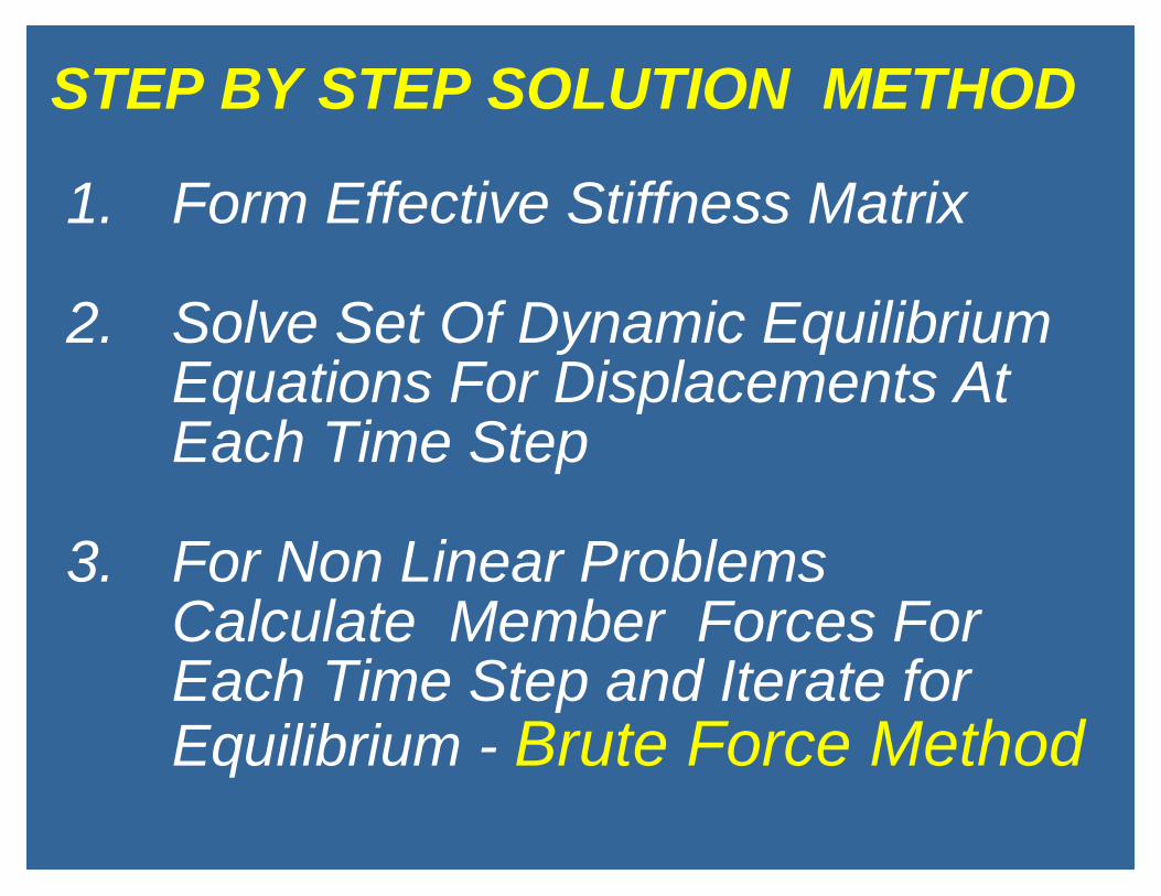
STEP BY STEP SOLUTION METHOD

1. Form Effective Stiffness Matrix

2. Solve Set Of Dynamic Equilibrium Equations For Displacements At Each Time Step

3. For Non Linear ProblemsCalculate Member Forces For Each Time Step and Iterate for Equilibrium - Brute Force Method

MODE SUPERPOSITION METHOD1. Generate Orthogonal Dependent

Vectors And Frequencies

2. Form Uncoupled Modal EquationsAnd Solve Using An Exact MethodFor Each Time Increment.

3. Recover Node DisplacementsAs a Function of Time

4. Calculate Member Forces As a Function of Time

GENERATION OF LOAD

DEPENDENT RITZ VECTORS1. Approximately Three Times Faster Than

The Calculation Of Exact Eigenvectors

2. Results In Improved Accuracy Using ASmaller Number Of LDR Vectors

3. Computer Storage Requirements Reduced

4. Can Be Used For Nonlinear Analysis ToCapture Local Static Response

STEP 1. INITIAL CALCULATION

A. TRIANGULARIZE STIFFNESS MATRIX

B. DUE TO A BLOCK OF STATIC LOAD VECTORS, f,SOLVE FOR A BLOCK OF DISPLACEMENTS, u,

K u = f

C. MAKE u STIFFNESS AND MASS ORTHOGONAL TO FORM FIRST BLOCK OF LDL VECTORS V 1

V1T M V1 = I

STEP 2. VECTOR GENERATIONi = 2 . . . . N Blocks

A. Solve for Block of Vectors, K Xi = M Vi-1

B. Make Vector Block, Xi , Stiffness and Mass Orthogonal - Yi

C. Use Modified Gram-Schmidt, Twice, toMake Block of Vectors, Yi , Orthogonalto all Previously Calculated Vectors - Vi

STEP 3. MAKE VECTORS STIFFNESS ORTHOGONAL

A. SOLVE Nb x Nb Eigenvalue Problem

[ VT K V ] Z = [ w2 ] Z

B. CALCULATE MASS AND STIFFNESS ORTHOGONAL LDR VECTORS

VR = V Z =

Φ

10 AT 12" = 240"

100 pounds

FORCE

TIME

DYNAMIC RESPONSE OF BEAM

MAXIMUM DISPLACEMENTNumber of Vectors Eigen Vectors Load DependentVectors 1 0.004572 (-2.41) 0.004726 (+0.88)

2 0.004572 (-2.41) 0.004591 ( -2.00)

3 0.004664 (-0.46) 0.004689 (+0.08)

4 0.004664 (-0.46) 0.004685 (+0.06)

5 0.004681 (-0.08) 0.004685 ( 0.00)

7 0.004683 (-0.04)

9 0.004685 (0.00)

( Error in Percent)

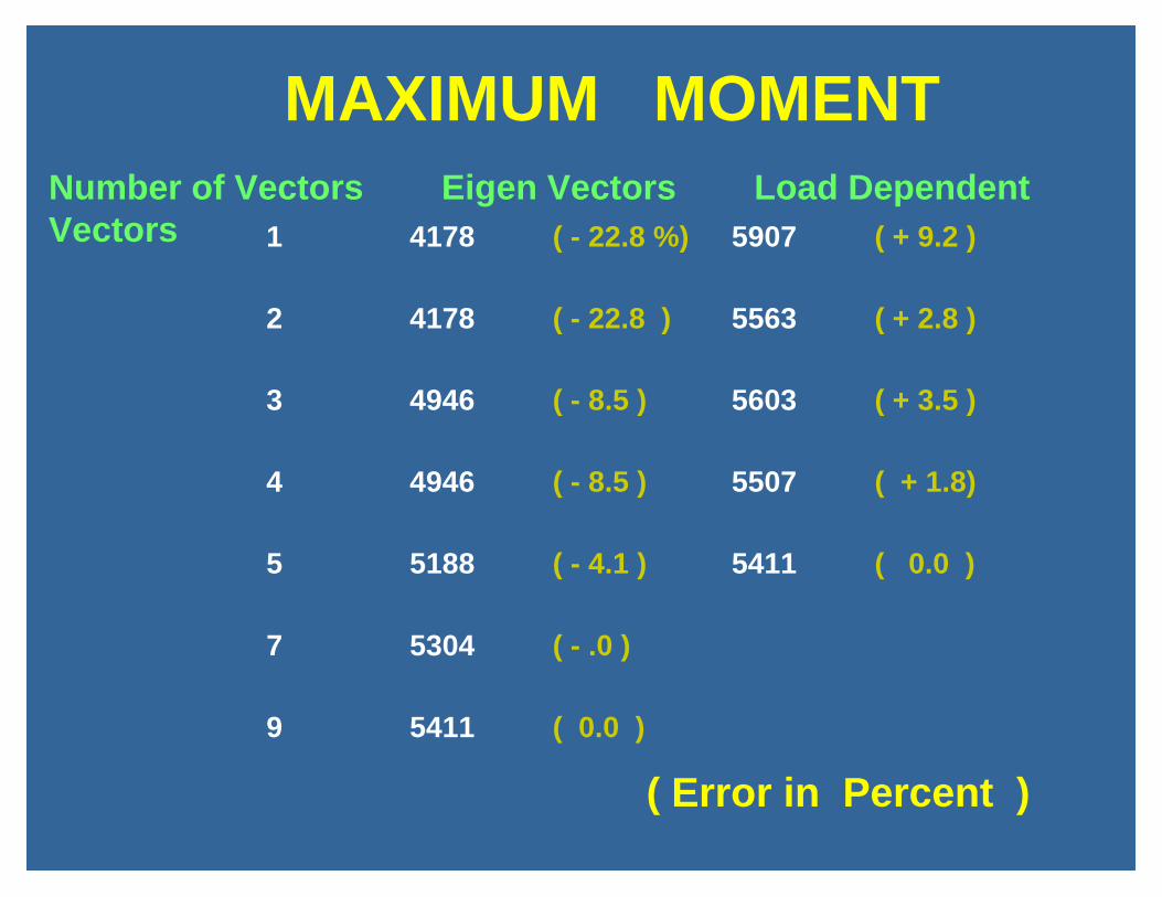
MAXIMUM MOMENTNumber of Vectors Eigen Vectors Load DependentVectors 1 4178 ( - 22.8 %) 5907 ( + 9.2 )

2 4178 ( - 22.8 ) 5563 ( + 2.8 )

3 4946 ( - 8.5 ) 5603 ( + 3.5 )

4 4946 ( - 8.5 ) 5507 ( + 1.8)

5 5188 ( - 4.1 ) 5411 ( 0.0 )

7 5304 ( - .0 )

9 5411 ( 0.0 )

( Error in Percent )

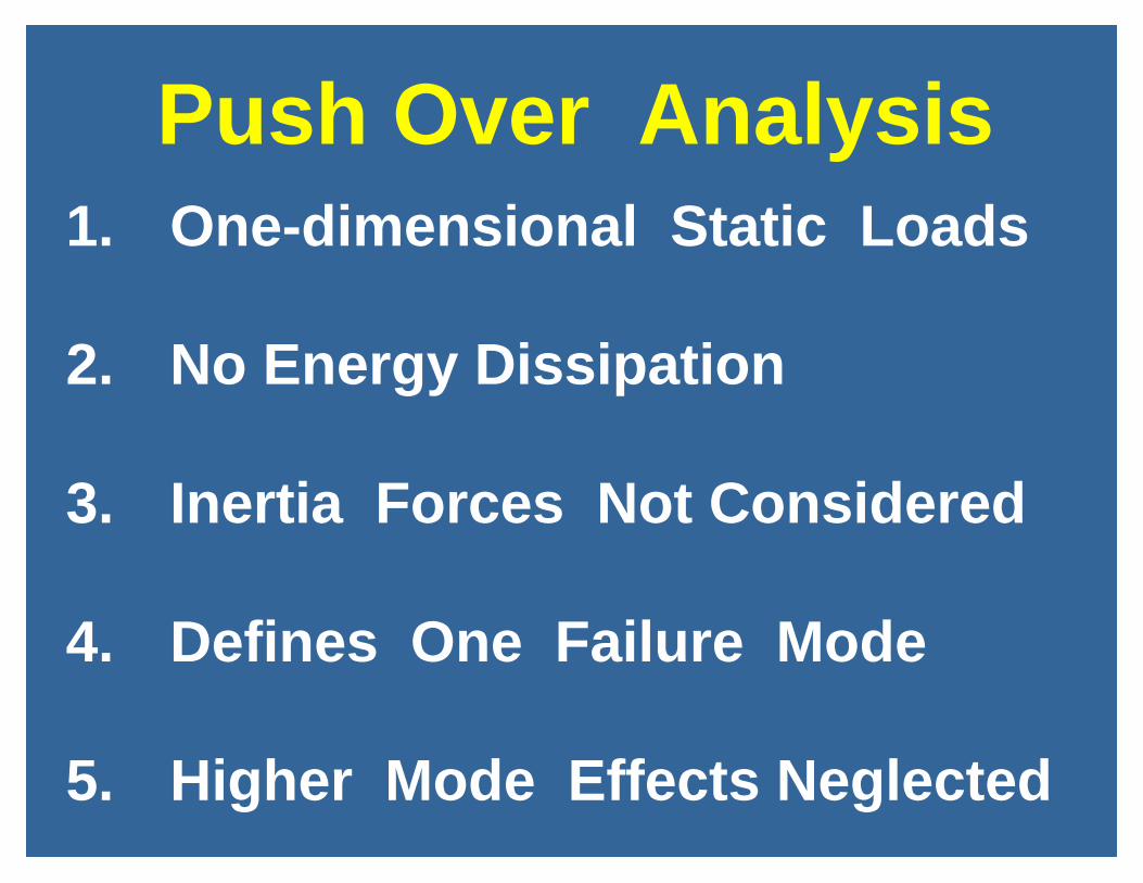
Push Over Analysis1. One-dimensional Static Loads

2. No Energy Dissipation

3. Inertia Forces Not Considered

4. Defines One Failure Mode

5. Higher Mode Effects Neglected

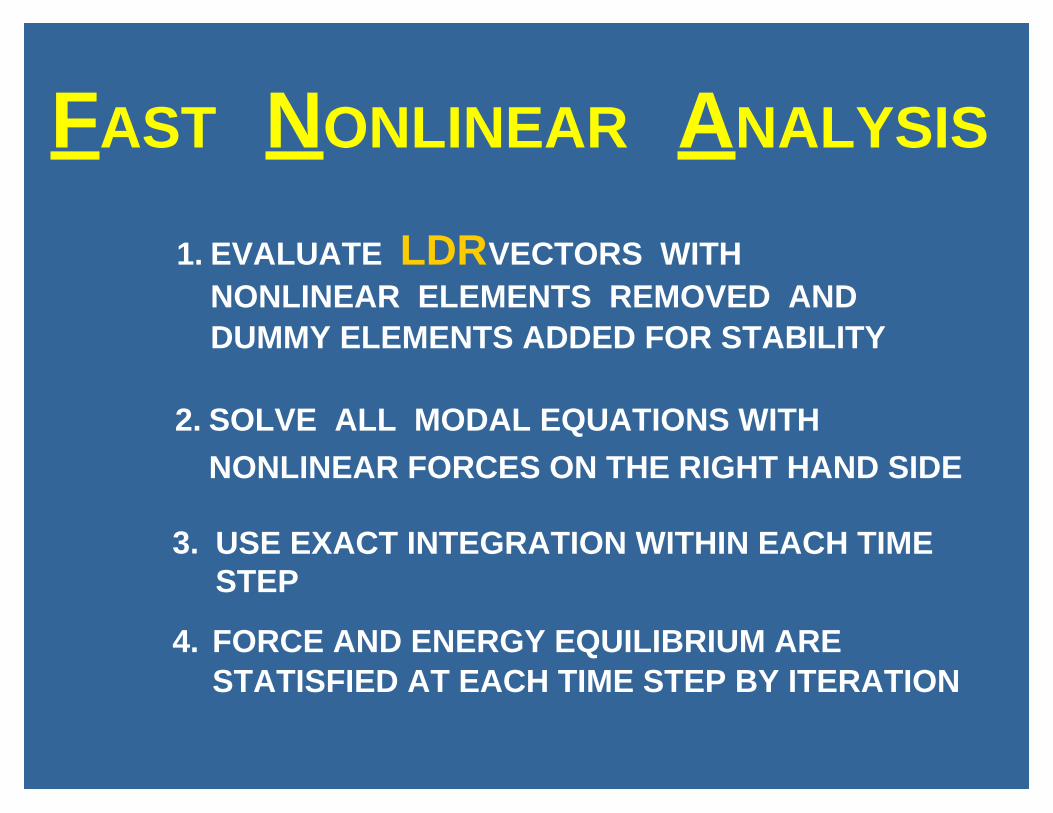
FAST NONLINEAR ANALYSIS

1. EVALUATE LDR VECTORS WITHNONLINEAR ELEMENTS REMOVED ANDDUMMY ELEMENTS ADDED FOR STABILITY

2. SOLVE ALL MODAL EQUATIONS WITH

NONLINEAR FORCES ON THE RIGHT HAND SIDE

USE EXACT INTEGRATION WITHIN EACH TIMESTEP

4. FORCE AND ENERGY EQUILIBRIUM ARESTATISFIED AT EACH TIME STEP BY ITERATION

3.

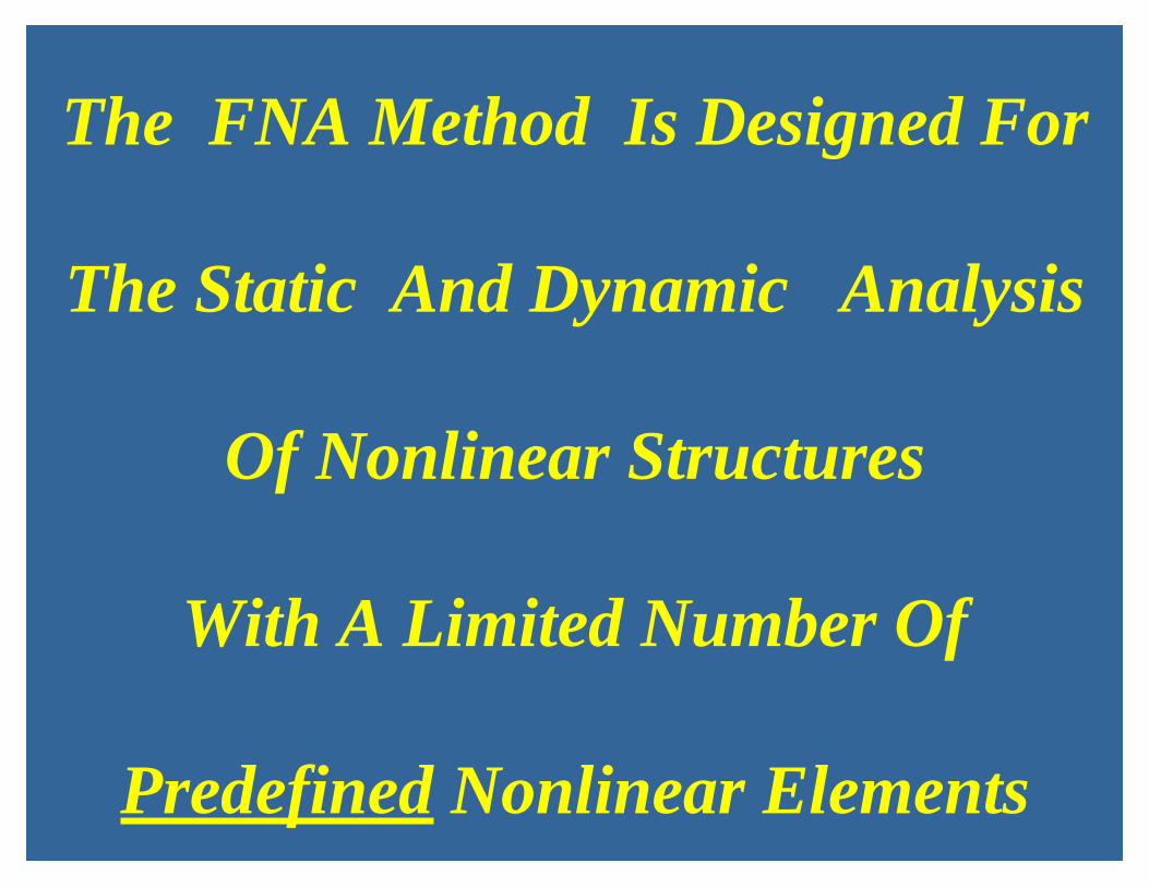
The FNA Method Is Designed For

The Static And Dynamic Analysis

Of Nonlinear Structures

With A Limited Number Of

Predefined Nonlinear Elements

Isolators

BASE ISOLATION

BUILDINGIMPACTANALYSIS

FRICTIONDEVICE

CONCENTRATEDDAMPER

NONLINEARELEMENT

GAP ELEMENT

TENSION ONLY ELEMENT

BRIDGE DECK ABUTMENT

P L A S T I CH I N G E S

2 ROTATIONALDOF

DEGRADING STIFFNESS ?

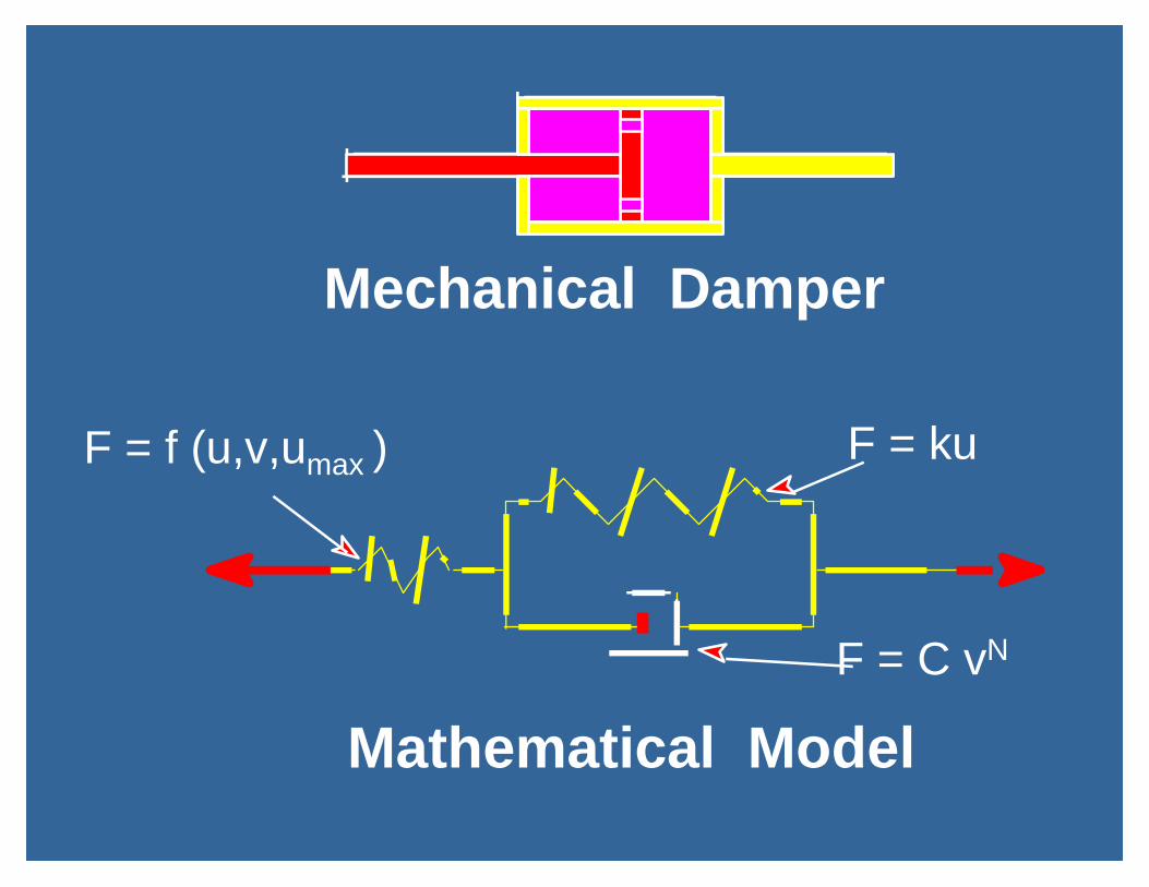
Mechanical Damper

Mathematical Model

F = C vN

F = kuF = f (u,v,umax )

LINEAR VISCOUS DAMPINGDOES NOT EXIST IN NORMAL STRUCTURESAND FOUNDATIONS

5 OR 10 PERCENT MODAL DAMPINGVALUES ARE OFTEN USED TO JUSTIFYENERGY DISSIPATION DUE TO NONLINEAREFFECTS

IF ENERGY DISSIPATION DEVICES ARE USEDTHEN 1 PERCENT MODAL DAMPING SHOULDBE USED FOR THE ELASTIC PART OFTHE STRUCTURE - CHECK ENERGYPLOTS

103 FEET DIAMETER - 100 FEET HEIGHT

ELEVATED WATERSTORAGE TANK

NONLINEARDIAGONALS

BASEISOLATION

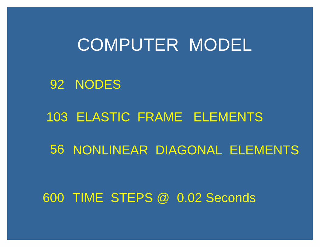
COMPUTER MODEL

92 NODES

103 ELASTIC FRAME ELEMENTS

56 NONLINEAR DIAGONAL ELEMENTS

600 TIME STEPS @ 0.02 Seconds

COMPUTER TIMEREQUIREMENTS

PROGRAM

( 4300 Minutes )ANSYS INTEL486

3 Days

ANSYS CRAY 3 Hours ( 180 Minutes )

SADSAP INTEL 486 2 Minutes

( B Array was 56 x 20 )

Nonlinear Equilibrium Equations

M a + Cv + Ku + FN = FOr

M a + Cv + Ku = F - FN

WhereFN = The Global Node Loads due to the Forces in the Nonlinear Elements

Nonlinear Equilibrium Equations

M a + Cv + [ K + kE ] u = F - FN + kE u

Where

kE = The Effective Linear Stiffness of the Nonlinear Elements are of arbitrary values for zero damping

Summary Of FNA Method

1. Calculate Ritz Vectors for StructureWith the Nonlinear Elements Removed.

2. These Vectors Satisfy the FollowingOrthogonality Properties

φ φTK = Ω2 φ φTM I=

3. The Solution Is Assumed to Be a LinearCombination of the LDR Vectors. Or,

Which Is the StandardMode Superposition Equation

∑∑====n

nn tytYtu )()()( φφ

Remember the LDR Vectors Are a LinearCombination of the Exact Eigenvectors;Plus, the Static Displacement Vectors.

No Additional Approximations Are Made.

4. A typical modal equation is uncoupled.However, the modes are coupled by theunknown nonlinear modal forces whichare of the following form:

5. The deformations in the nonlinear elementscan be calculated from the followingdisplacement transformation equation:

f Fn n n= φ

δ = A u

6. Since the deformations inthe nonlinear elements can be expressedin terms of the modal response by

Where the size of the array is equal tothe number of deformations times the number of LDR vectors.

The array is calculated only once priorto the start of mode integration.

THE ARRAY CAN BE STORED IN RAM

)()( tYtu φ==

δ φ( ) ( ) ( )t A Y t BY t= =

B

B

B

7. The nonlinear element forces arecalculated, for iteration i , at the endof each time step t

Equation Modal of SolutionNew

Loads Modal Nonlinear

History Element of Function

Elements Nonlinear

in nsDeformatio

==

====

==

====

++ )(

)(t

T)(N

)(

)(t

Y

YBf

P

BY

1

)(

it

ii

it

iit

t

δ

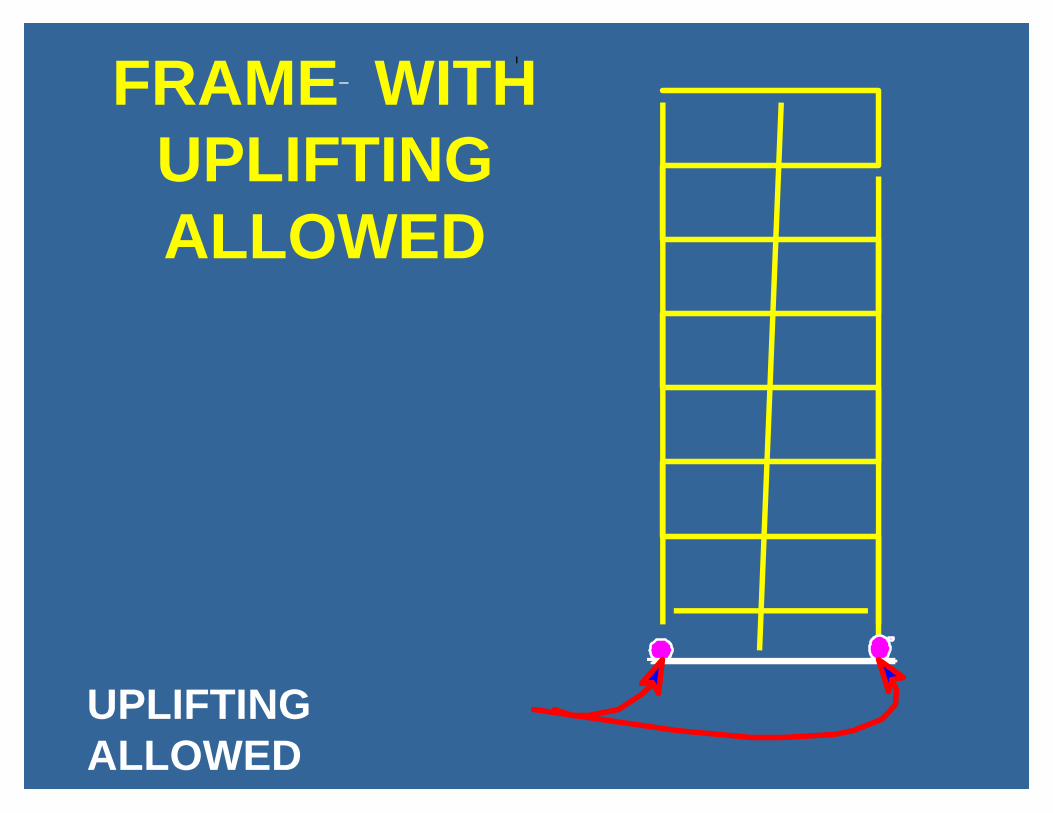
FRAME WITHUPLIFTINGALLOWED

UPLIFTINGALLOWED

Four Static Load ConditionsAre Used To Start The

Generate of LDR Vectors

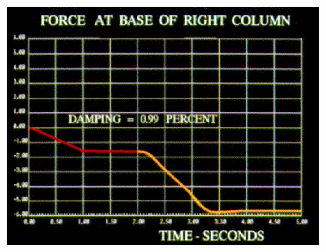
EQ DL Left Right

TIME - Seconds

DEAD LOAD

LATERAL LOAD

LOAD

0 1.0 2.0 3.0 4.0 5.0

NONLINEAR STATIC ANALYSIS50 STEPS AT dT = 0.10 SECONDS

Advantages Of The FNA Method

1. The Method Can Be Used For BothStatic And Dynamic Nonlinear Analyses

2. The Method Is Very Efficient And Requires A Small Amount Of Additional Computer Time As Compared To Linear Analysis

2. The Method Can Easily Be IncorporatedInto Existing Computer Programs ForLINEAR DYNAMIC ANALYSIS.

FUTURE DEVELOPMENTS FORSAP2000

1. ADDITIONAL NONLINEAR ELEMENTScrush and yield elementsdegrading stiffness elementsgeneral CABLE element

2. SUBSTRUCTURE OPTION

3. SOIL STRUCTURE INTERACTION

4. FULID - STRUCTURE INTERACTION

5. ADDITIONAL DOCUMENTATIONAND EXAMPLES

EXAMPLE ON THE USE OF

SUBSTRUCTURE ANALYSIS

LINEAR AND NONLINEAR ANALYSIS

OF THE

RICHMOND-SAN RAFAEL BRIDGE

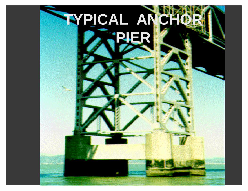
TYPICAL ANCHORPIER

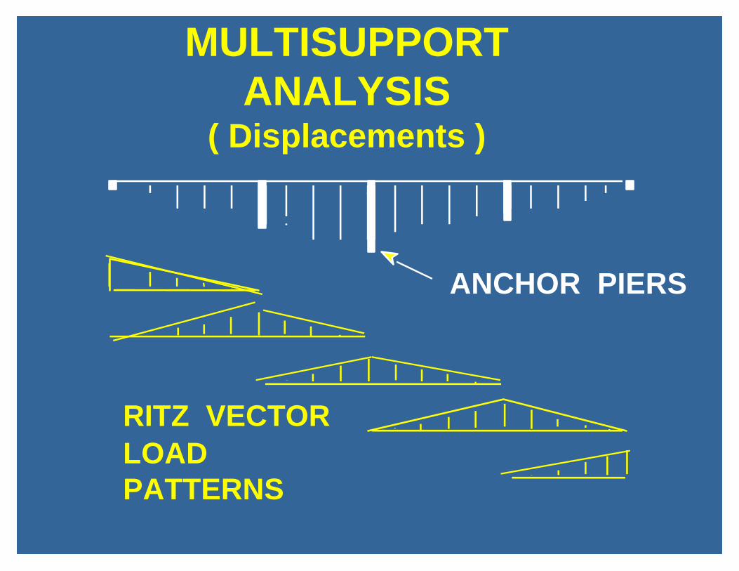
MULTISUPPORTANALYSIS

( Displacements )

ANCHOR PIERS

RITZ VECTORLOADPATTERNS

SUBSTRUCTURE PHYSICS

JOINT REACTIONS( Retained DOF )

MASS POINTS and

MASSLESS JOINT( Eliminated DOF )

Stiffness Matrix Size = 3 x 16 = 48

"a"

"b"

SUBSTRUCTURESUBROUTINE

SEE FORTRAN LISTING

k k

k ka a a b

b a b b

ADVANTAGES IN THEUSE OF SUBSTRUCTURES

1. FORM OF MESH GENERATION

2. LOGICAL SUBDIVISION OF WORK

3. MANY SHORT COMPUTER RUNS

4. RERUN ONLY SUBSTRUCTURES WHICH WERE REDESIGNED

5. PARALLEL POST PROCESSINGUSING NETWORKING

ECCENTRICALLY BRACEDFRAME

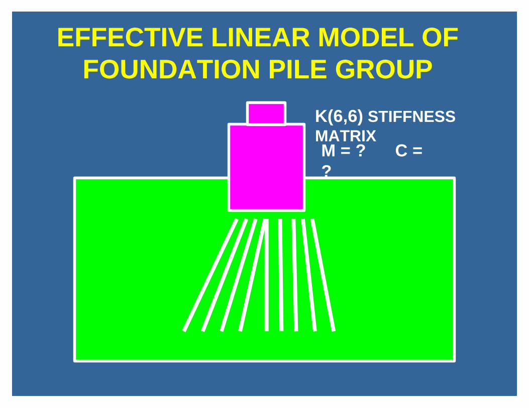
EFFECTIVE LINEAR MODEL OFFOUNDATION PILE GROUP

K(6,6) STIFFNESSMATRIXM = ? C =?

NONLINEAR MODEL OFFOUNDATION PILE GROUP ??

CS = VS / m

CN = VN / m

SITE ANALYSIS - SHAKE

1. ONE-DIMENSIONAL ANALYSIS

2. EFFECTIVE MODULUS andCONSTANT VISCOUS DAMPINGNOT A FUNCTION OF TIME

3. PERMANENT SET NOT POSSIBLE

4. ARE THESE APPROXIMATIONSNECESSARY ? Use SAP 2000

FEATHER Structure

RIGID BLOCKFoundation

STRUCTURAL ENGINEER'S VIEW OF SOIL-STRUCTURE SYSTEM

RIGID BLOCKStructure

FEATHER PILLOWFoundation

GEOTECHNICAL ENGINEER'S VIEWOF

SOIL-STRUCTURE SYSTEM

WHAT IS THE MOST SIGNIFICANTBARRIER TO PRODUCING GOOD

SOLUTIONS OF SOIL-STRUCTUREINTERACTION PROBLEMS?

SITE RESPONSE AND STRUCTURALENGINEERING ARE CONDUCTED ATDIFFERENT LOCATIONS (OFFICES)

USING DIFFERENT NUMERICALMETHODS AND APPROXIMATIONS

WIND RESPONSE

OF

TALL BUILDINGS

Base IsolationOr Uplift

Dampers Plastic Hinge - Frictionand Gap Elements

ENERGY DISSIPATION SYSTEMS

Dynamic Wind Analysis1. Random Vibration .

A. Classical Approach.

B. Linear Analysis Only

2. Time History Response.

A. Exact For Given Periodic Loading

B. Non-linear Analysis Is Possible

C. Can Perform Code Checks As

A Function Of Time

0.1

)1()1(

≤≤

−−

++

−−

++

byF

eyF

af

byf

myC

bxF

exF

af

bxf

mxC

aF

af

Weakness Of The ResponseSpectrum Methods

The Use Of The Maximum Peak Values Offa , fbx and fby Produces An Inconsistent Design

Axial Members Are Under Designed Compared ToBi-Axial Bending Members

SOLUTION ?

Use Design Checks As A Function Of Time

Determination Of Wind Forces

As Function Of Time

1. ANALYSIS AND FORMULAS

2. FIELD MEASUREMENTS

3. WIND TUNNEL TESTS

ii tt )()( ∑∑== gfR

PRINCIPAL

WIND DIRECTION

CROSS

WIND DIRECTION

)(tα

WIND FORCES ACTING ON BUILDINGS

F(t)iBUILDING

VERTICAL DISTRIBUTIONOF WIND FORCES

T

pT pT pT pTTime

F(t)

MeanWindPressure

TP = 10 TO 50 Seconds

PERIODIC WIND LOADING

y(t) = zero initial conditions using. piece-wise exact integration

x(t) = unknown initial conditions

z(t) =y(t) + x(t) .. = exact periodic solution

TP

+

)0(

)0(

x

x

& )(

)(

p

p

Tx

Tx

&

)(

)(

p

p

Tz

Tz

&

)(

)(

p

p

Ty

Ty

&

)(

)(

p

p

Tz

Tz

&

Conversion Of Transient SolutionTo Periodic Solution

PARALLEL ENGINEERING

AND

PARALLEL COMPUTERS

ONE PROCESSOR ASSIGNED TO EACH JOINT

ONE PROCESSOR ASSIGNEDTO EACH MEMBER

1

2

3

1 23

PARALLEL STRUCTURALANALYSIS

DIVIDE STRUCTURE INTO "N" DOMAINS

FORM AND SOLVE EQUILIBRIUM EQ.

FORM ELEMENT STIFFNESS

IN PARALLEL FOR

"N" SUBSTRUCTURES

EVALUATE ELEMENT

FORCES IN PARALLEL

IN "N" SUBSTRUCTURES

NONLINEAR LOOP

TYPICALCOMPUTER

FINAL REMARKS1. LINEAR AND NONLINEAR DYNAMIC ANALYSES CAN BE CONDUCTED, OF LARGE STRUCTURES,

USING INEXPENSIVE PERSONAL COMPUTERS

2. SUBSTRUCTURE METHODS HAS MANYADVANTAGES FOR LARGE STRUCTURES

3. TIME-HISTORY DYNAMIC WIND ANALYSES CAN NOW BE CONDUCTED OF STRUCTURES

4. NEW NUMERICAL METHODS ALLOW FOR

FAST NONLINEAR ANALYSISFOR MANY STRUCTURES SUBJECTED TOEARTHQUAKE LOADING

ED WILSON ON-LINE\www\ed@csiberkeley.com

orFAX or PHONE1-510-526-4170

___________________________________________________________________________________________

TO ORDER $25 BOOK“THREE-DIMENSIONAL STATIC AND DYNAMIC ANALYSIS OF

STRUCTURES” by Edward L. WILSON

Computers And Structures, Inc.1995 University Avenue

Berkeley, Ca 94704 USA

(510) 845-2177