Dynamic Signal Analysis Basics - PROGRAMTEH Signal Analysis Basics.pdf · DYNAMIC SIGNAL ANALYSIS BASICS COPYRIGHT © 2009 CRYSTAL INSTRUMENTS.ALL RIGHTS RESERVED. PAGE 4 FREQUENCY

DYNAMIC SIGNAL ANALYSIS BASICS

COPYRIGHT © 2009 CRYSTAL INSTRUMENTS. ALL RIGHTS RESERVED. PAGE 1

Dynamic Signal Analysis Basics

James Zhuge, Ph.D., President

Crystal Instruments Corporation

4633 Old Ironsides Drive, Suite 304

Santa Clara, CA 95054, USA

www.go-ci.com

(Part of CoCo-80 User’s Manual)

http://www.go-ci.com/



Table of Contents

FREQUENCY ANALYSIS .................................................................................................................................... 4 Basic Theory of FFT Frequency Analysis ............................................................................................................. 4

Introduction ..................................................................................................................................................... 4 Fourier Transform ........................................................................................................................................... 5 Data Windowing ............................................................................................................................................. 5 Linear Spectrum ............................................................................................................................................. 6 Power Spectrum ............................................................................................................................................. 8 Spectrum Types ............................................................................................................................................. 9 Cross Spectrum ............................................................................................................................................ 13 Frequency Response and Coherence Function ........................................................................................... 14

Data Window Selection ....................................................................................................................................... 15 Leakage Effect.............................................................................................................................................. 15 Data Window Formula .................................................................................................................................. 17 How to Choose the Right Data Window ....................................................................................................... 18 Guidelines of Choosing Data Windows ........................................................................................................ 21

Averaging Techniques ........................................................................................................................................ 21 Linear Averaging .......................................................................................................................................... 21 Moving Linear Averaging .............................................................................................................................. 22 Exponential Averaging.................................................................................................................................. 23 Peak-Hold ..................................................................................................................................................... 23 Linear Spectrum versus Power Spectrum Averaging ................................................................................... 23 Spectrum Estimation Error ........................................................................................................................... 24 Overlap Processing ...................................................................................................................................... 25 Single Degree of Freedom System .............................................................................................................. 26 dB and Linear Magnitude ............................................................................................................................. 27

TRANSIENT CAPTURE AND HAMMER TESTING .......................................................................................... 29 Transient Capture ............................................................................................................................................... 29 Impact Hammer Testing ..................................................................................................................................... 29

Impact Test Analyzer Settings ...................................................................................................................... 31 References .......................................................................................................................................................... 32



Table of Figures

Figure 1. Sine wave with Hanning window applied to the spectrum. __________________________________ 7 Figure 2. Hanning windowing function applied to a pure sine tone. ___________________________________ 8 Figure 3. Flow chart to determine measurement technique for various signal types. _____________________ 10 Figure 4. A sine wave is measured with EUpk spectrum unit. The sine waveform has a 1V amplitude. _______ 11 Figure 5. A sine wave is measured with EUrms spectrum unit. The peak reading is 0.707V. The sine waveform has a 1V amplitude. _______________________________________________________________________________ 11 Figure 6. A sine wave is measured with (EUrms)

2 spectrum unit. The peak reading is 0.5V

2. The sine waveform

has a 1V amplitude. _______________________________________________________________________________ 12 Figure 7. White noise with 1 volt RMS amplitude displays as 100 u Vrms

2/Hz. ___________________________ 12 Figure 8. Random signal with 1 volt RMS amplitude and Energy Spectrum Density format. ________________ 13 Figure 9. Frequency response function computation. _____________________________________________ 14 Figure 10. Illustration of a non-periodic signal resulting from sampling. _______________________________ 15 Figure 11. Sine spectrum with no leakage. _____________________________________________________ 16 Figure 12. Sine spectrum with significant leakage. _______________________________________________ 16 Figure 13. Sine spectrum with Flattop windowing function. ________________________________________ 17 Figure 14. Spectral shape of common windowing functions. _______________________________________ 19 Figure 15. Window frequency response showing main lobe and side lobes. ___________________________ 20 Figure 16. Illustration of moving linear average. _________________________________________________ 22 Figure 17. Illustration of overlap processing. ____________________________________________________ 25 Figure 18. SDOF system and their frequency response. ____________________________________________ 26 Figure 19. Step response of a SDOF system with different damping ratios._____________________________ 27 Figure 20. Show a 1Vpk sine signal in frequency domain with dB scaling. _____________________________ 28 Figure 21. A 1Vpk sine signal in frequency domain with LogMag scaling. ______________________________ 28 Figure 22. Transient capture operation on CoCo. ________________________________________________ 29 Figure 23. Illustration of a typical impact test and signal processing. _________________________________ 30 Figure 24. Typical impact test data. Top left shows excitation force impulse time signal, top right shows response acceleration time signal and bottom shows FRF spectrum. _________________________________________________ 31



FREQUENCY ANALYSIS

Basic Theory of FFT Frequency Analysis

Introduction

DSA, often referred to Dynamic Signal Analysis or Dynamic Signal Analyzer depending on the context, is an application area of digital signal processing technology. Compared to general data acquisition and time domain analysis, DSA instruments and math tools focus more on the dynamic aspect of the signals such as frequency response, dynamic range, total harmonic distortion, phase match, amplitude flatness etc.. In recent years, time domain data acquisition devices and DSA instruments have gradually converged together. More and more time domain instruments, such as oscilloscopes, can do frequency analysis while more and more dynamic signal analyzers can do long time data recording. DSA uses various different technology of digital signal processing. Among them, the most fundamental and popular technology is based on the so called the Fast Fourier Transform (FFT). The FFT transforms the time domain signals into the frequency domain. To perform FFT-based measurements, however, you need to understand the fundamental issues and computations involved. This Chapter describes some of the basic signal analysis computations, discusses antialiasing and acquisition front end for FFT-based signal analysis, explains how to use windowing functions correctly, explains some spectrum computations, and shows you how to use FFT-based functions for some typical measurements. In this Chapter we will use standard notations for different signals. Each type of signal will be represented by one specific letter. For example, “G” stands for a one-side power spectrum, while “H” stands for a transfer function. The following table defines the symbols used in this Chapter: Cyx Coherence function between input signal x and output signal y Gxx Auto-spectral function (one-sided) of signal x Gyx Cross-spectral function (one-sided) between input signal x and output signal y Hyx Transfer function between input signal x and output signal y k Index of a discrete sample Rxx Auto-correlation function of signal x Ryx Cross-correlation function between input signal x and output signal y Sx Linear spectral function of signal x Sxx Instantaneous auto-spectral function (one-sided) of signal x Syx Instantaneous cross-spectral function (one-sided) between input signal x and output

signal y t Time variable x(t) Time history record X(f) Fourier Transform of time history record



Fourier Transform

Digital signal processing technology includes FFT based frequency analysis, digital filters and many other topics. This chapter introduces the FFT based frequency analysis methods that are widely used in all dynamic signal analyzers. CoCo has fully utilized the FFT frequency analysis methods and various real time digital filters to analyze the measurement signals. The Fourier Transform is a transform used to convert quantities from the time domain to the frequency domain and vice versa, usually derived from the Fourier integral of a periodic function when the period grows without limit, often expressed as a Fourier transform pair. In the classical sense, a Fourier transform takes the form of

𝑋 𝑓 = 𝑥 𝑡 𝑒−𝑗2𝜋𝑓𝑡 𝑑𝑡∞

−∞

where x(t) continuous time waveform f frequency variable

j complex number X(f) Fourier transform of x(t) Mathematically the Fourier Transform is defined for all frequencies from negative to positive infinity. However, the spectrum is usually symmetric and it is common to only consider the single-sided spectrum which is the spectrum from zero to positive infinity. For discrete sampled signals, this can be expressed as

𝑋 𝑘 = 𝑥 𝑘 𝑒−𝑗2𝜋𝑘𝑛 /𝑁

𝑁−1

𝑛=0

where x(k) samples of time waveform n running sample index N total number of samples or “frame size” k finite analysis frequency, corresponding to “FFT bin centers” X(k) discrete Fourier transform of x(k) In most DSA products, a Radix-2 DIF FFT algorithm is used, which requires that the total number of samples must be a power of 2 (total number of samples in FFT = 2

m , where m is an integer).

Data Windowing

The Fourier Transform assumes that the time signal is periodic and infinite in duration. When only a portion of a record is analyzed the record must be truncated by a data window to preserve the frequency characteristics. A window can be expressed in either the time domain or in the frequency domain, although the former is more common. To reduce the edge effects, which cause leakage, a window is often given a shape or weighting function. For example, a window can be defined as w(t) = g(t) -T/2 < t < T/2 = 0 elsewhere



where g(t) is the window weighting function and T is the window duration. The data analyzed, x(t) are then given by x(t) = w(t) x(t)’ where x(t)’ is the original data and x(t) is the data used for spectral analysis. A window in the time domain is represented by a multiplication and hence, is a convolution in the frequency domain. A convolution can be thought of as a smoothing function. This smoothing can be represented by an effective filter shape of the window; i.e., energy at a frequency in the original data will appear at other frequencies as given by the filter shape. Since time domain windows can be represented as a filter in the frequency domain, the time domain windowing can be accomplished directly in the frequency domain. In most DSA products, rectangular, Hann, Flattop and several other data windows are used; Rectangular Window

w(k) = 1 0 k N-1 Hann Window

w(k) = 0.5 * (1 - cos (2k /(N-1) ) 0 k N-1 Because creating data window attenuates a portion of the original data, a certain amount of correction has to be made in order to get an un-biased estimation of the spectra. In linear spectral analysis, an Amplitude Correction is applied; in power spectral measurements, an Energy Correction is applied. See the sections below for details.

Linear Spectrum

A linear spectrum is the Fourier transform of windowed time domain data. The linear spectrum is useful for analyzing periodic signals. You can extract the harmonic amplitude by reading the amplitude values at those harmonic frequencies. An averaging technique is often used in the time domain when synchronized triggering is applied. Or equivalently, the averaging can be applied to the complex FFT spectra. Because the averaging is taking place in the linear spectrum domain, or equivalently, in the time domain, based on the principles of linear transform, averaging make no sense unless a synchronized trigger is used. Most DSA products use the following steps to compute a linear spectrum: Step 1 First a window is applied: x(t) = w(t) x(t)’ where x(t)’ is the original data and x(t) is the data used for the Fourier transform. Step 2



The FFT is applied to x(t) to compute X(k), as described above. Step 3 Averaging is applied to X(k). Here Averaging can be either an Exponential Average or Stable Average. Result is Sx’. Sx’ = Average ( X(k) ) Step 4 To get a single-sided spectrum, double the value for symmetry about DC. An Amplitude Correction factor is applied to Sx’ so that the final result has an un-biased reading at the harmonic frequencies.

Sx = 2 Sx’ / AmpCorr where AmpCorr is the amplitude correction factor, defined as:

𝐴𝑚𝑝𝐶𝑜𝑟𝑟 = 𝑤 𝑘

𝑁−1

𝑘=0

where w(k) is the window weighting function. This correction will make the peak or RMS reading of a sine wave at specific frequency correct regardless of which data window is applied. For example, if a 1.0 volt amplitude 1kHz sine wave sampled at 6.4kHz is analyzed with a Linear Spectrum with Hann window, you will get following the spectral shape:

Figure 1. Sine wave with Hanning window applied to the spectrum.

The top picture is the digitized time waveform. The sine-wave is not smooth because of the low sampling rate relative to the frequency of the signal. However the well known Nyquist principle indicates that the frequency estimate from the FFT will be accurate as long as the sampling rate is



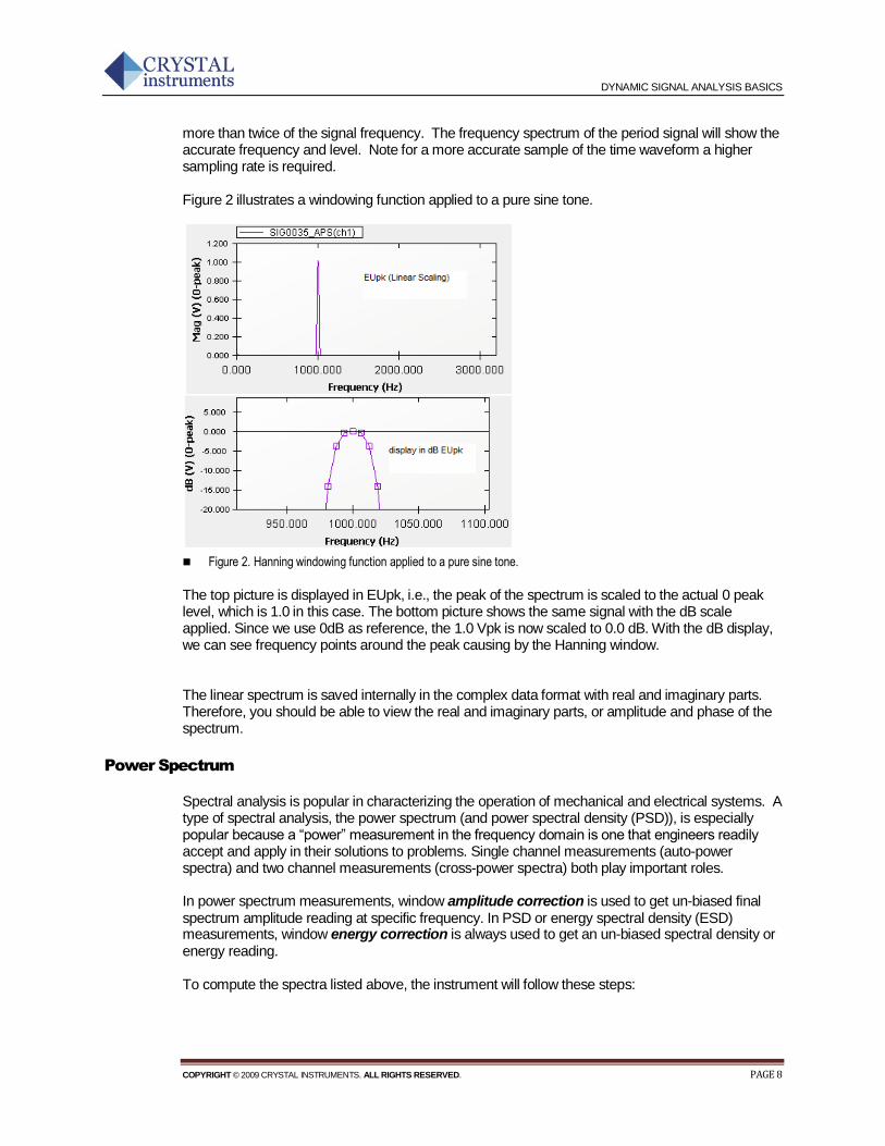
more than twice of the signal frequency. The frequency spectrum of the period signal will show the accurate frequency and level. Note for a more accurate sample of the time waveform a higher sampling rate is required. Figure 2 illustrates a windowing function applied to a pure sine tone.

Figure 2. Hanning windowing function applied to a pure sine tone.

The top picture is displayed in EUpk, i.e., the peak of the spectrum is scaled to the actual 0 peak level, which is 1.0 in this case. The bottom picture shows the same signal with the dB scale applied. Since we use 0dB as reference, the 1.0 Vpk is now scaled to 0.0 dB. With the dB display, we can see frequency points around the peak causing by the Hanning window. The linear spectrum is saved internally in the complex data format with real and imaginary parts. Therefore, you should be able to view the real and imaginary parts, or amplitude and phase of the spectrum.

Power Spectrum

Spectral analysis is popular in characterizing the operation of mechanical and electrical systems. A type of spectral analysis, the power spectrum (and power spectral density (PSD)), is especially popular because a “power” measurement in the frequency domain is one that engineers readily accept and apply in their solutions to problems. Single channel measurements (auto-power spectra) and two channel measurements (cross-power spectra) both play important roles. In power spectrum measurements, window amplitude correction is used to get un-biased final spectrum amplitude reading at specific frequency. In PSD or energy spectral density (ESD) measurements, window energy correction is always used to get an un-biased spectral density or energy reading. To compute the spectra listed above, the instrument will follow these steps:



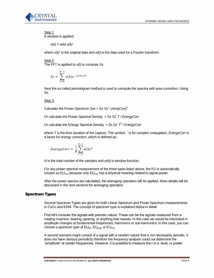
Step 1 A window is applied: x(k) = w(k) x(k)’ where x(k)’ is the original data and x(k) is the data used for a Fourier transform. Step 2 The FFT is applied to x(t) to compute Sx

𝑆𝑥 = 𝑥 𝑘 𝑒−𝑗2𝜋𝑘𝑛 /𝑁

𝑁−1

𝑛=0

Next the so called periodogram method is used to compute the spectra with area correction. Using Sx. Step 3 Calculate the Power Spectrum Sxx = Sx Sx

* / (AmpCorr)

2

Or calculate the Power Spectral Density = Sx Sx

* T / EnergyCorr

Or calculate the Energy Spectral Density = Sx Sx

* T

2 / EnergyCorr

where T is the time duration of the capture. The symbol

* is for complex conjugation. EnergyCorr is

a factor for energy correction, which is defined as:

𝐸𝑛𝑒𝑟𝑔𝑦𝐶𝑜𝑟𝑟 = 1

𝑁 𝑤 𝑘 2

𝑁−1

𝑘=0

N is the total number of the samples and w(k) is window function. For any power spectral measurement of the three types listed above, the EU is automatically chosen as EUrms because only EUrms has a physical meaning related to signal power. After the power spectra are calculated, the averaging operation will be applied. More details will be discussed in the next sections for averaging operation.

Spectrum Types

Several Spectrum Types are given for both Linear Spectrum and Power Spectrum measurements in CoCo and EDM. The concept of spectrum type is explained below in detail. First let’s consider the signals with periodic nature. These can be the signals measured from a rotating machine, bearing, gearing, or anything that repeats. In this case we would be interested in amplitude changes at fundamental frequencies, harmonics or sub-harmonics. In this case, you can choose a spectrum type of EUpk, EUpkpk or EUrms. A second scenario might consist of a signal with a random nature that is not necessarily periodic. It does not have obvious periodicity therefore the frequency analysis could not determine the “amplitude” at certain frequencies. However, it is possible to measure the r.m.s. level, or power



level, or power density level over certain frequency bands for such random signals. In this case, you must select one of the spectrum types of EUrms

2/Hz, or EUrms/sqrt(Hz), which is called power

spectral density, or root-mean squared density. A third scenario might consist of a transient signal. It is neither periodic, nor stably random. In this case, must select a spectrum type as EU

2S/Hz, which is called energy spectrum.

In many applications, the nature of the data cannot be easily classified. Care must be taken to interpret the data when different spectrum types are used. For example, in the environmental vibration simulation, a typical test uses multiple sine tones on top of random profile, which is called Sine-on-Random. In this type application, you have to observe the random portion of the data in the spectrum with EUrms

2/Hz and the sine portion of the data with EUpk.

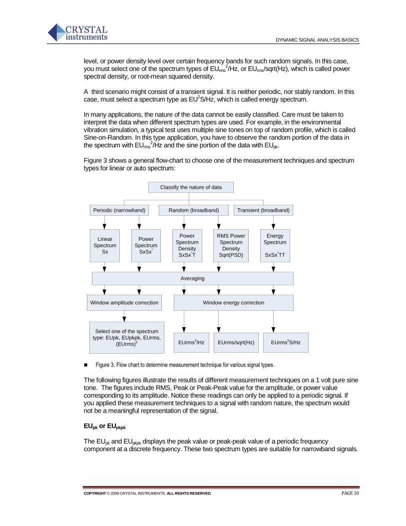
Figure 3 shows a general flow-chart to choose one of the measurement techniques and spectrum types for linear or auto spectrum:

Classify the nature of data

Periodic (narrowband) Random (broadband) Transient (broadband)

Linear

Spectrum

Sx

Power

Spectrum

SxSx*

Power

Spectrum

Density

SxSx*T

RMS Power

Spectrum

Density

Sqrt(PSD)

Energy

Spectrum

SxSx*TT

Window amplitude correction Window energy correction

Select one of the spectrum

type: EUpk, EUpkpk, EUrms,

(EUrms)2 EUrms

2/Hz EUrms/sqrt(Hz) EUrms

2S/Hz

Averaging

Figure 3. Flow chart to determine measurement technique for various signal types.

The following figures illustrate the results of different measurement techniques on a 1 volt pure sine tone. The figures include RMS, Peak or Peak-Peak value for the amplitude, or power value corresponding to its amplitude. Notice these readings can only be applied to a periodic signal. If you applied these measurement techniques to a signal with random nature, the spectrum would not be a meaningful representation of the signal. EUpk or EUpkpk The EUpk and EUpkpk displays the peak value or peak-peak value of a periodic frequency component at a discrete frequency. These two spectrum types are suitable for narrowband signals.



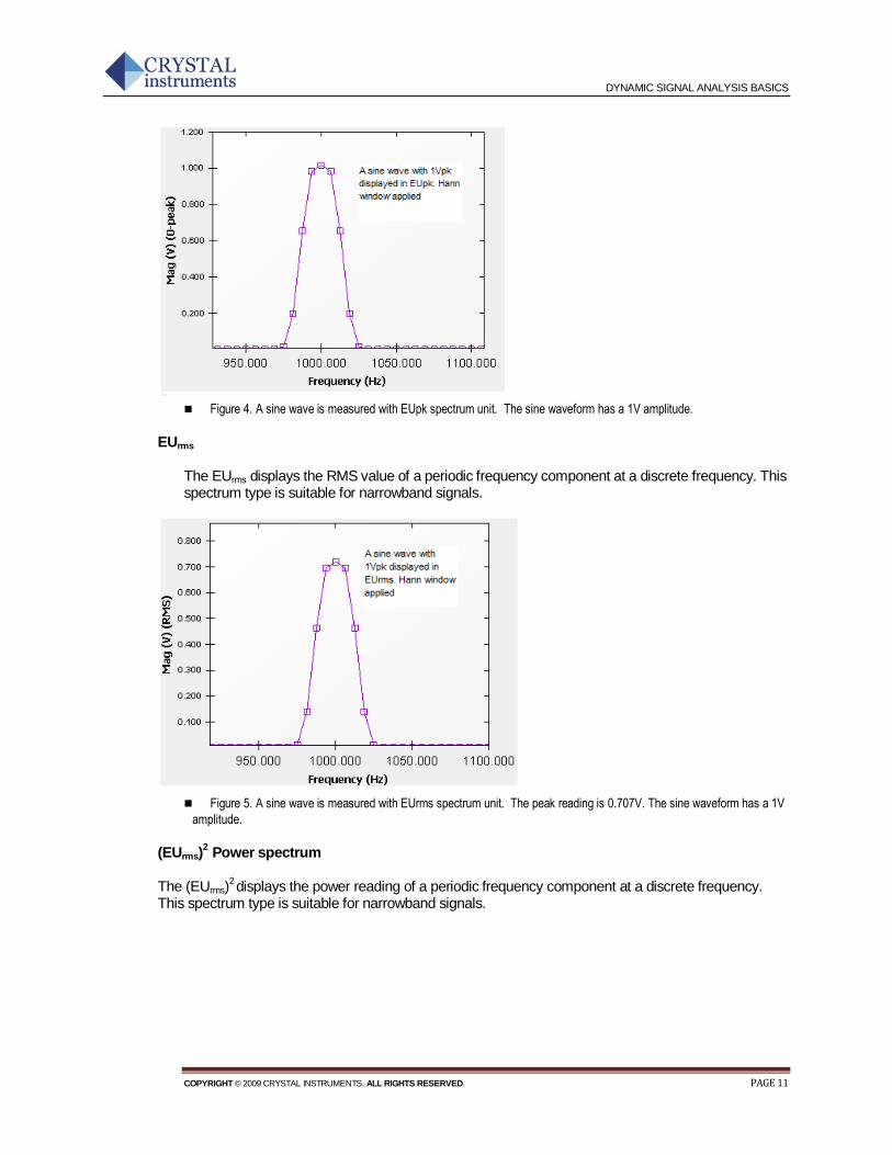
Figure 4. A sine wave is measured with EUpk spectrum unit. The sine waveform has a 1V amplitude.

EUrms The EUrms displays the RMS value of a periodic frequency component at a discrete frequency. This spectrum type is suitable for narrowband signals.

Figure 5. A sine wave is measured with EUrms spectrum unit. The peak reading is 0.707V. The sine waveform has a 1V

amplitude.

(EUrms)2

Power spectrum

The (EUrms)

2 displays the power reading of a periodic frequency component at a discrete frequency.

This spectrum type is suitable for narrowband signals.



Figure 6. A sine wave is measured with (EUrms)2 spectrum unit. The peak reading is 0.5V2. The sine waveform has a 1V

amplitude.

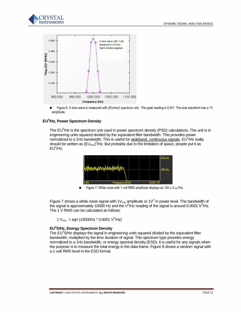
EU2/Hz, Power Spectrum Density The EU

2/Hz is the spectrum unit used in power spectrum density (PSD) calculations. The unit is in

engineering units squared divided by the equivalent filter bandwidth. This provides power normalized to a 1Hz bandwidth. This is useful for wideband, continuous signals. EU

2/Hz really

should be written as (EUrms)2/Hz. But probably due to the limitation of space, people put it as

EU2/Hz.

Figure 7. White noise with 1 volt RMS amplitude displays as 100 u Vrms2/Hz.

Figure 7 shows a white noise signal with 1Vrms amplitude or 1V

2 in power level. The bandwidth of

the signal is approximately 10000 Hz and the V2/Hz reading of the signal is around 0.0001 V

2/Hz.

The 1 V RMS can be calculated as follows:

1 Vrms = sqrt (10000Hz * 0.0001 V2/Hz)

EU

2S/Hz, Energy Spectrum Density

The EU2S/Hz displays the signal in engineering units squared divided by the equivalent filter

bandwidth, multiplied by the time duration of signal. This spectrum type provides energy normalized to a 1Hz bandwidth, or energy spectral density (ESD). It is useful for any signals when the purpose is to measure the total energy in the data frame. Figure 8 shows a random signal with a 1 volt RMS level in the ESD format.



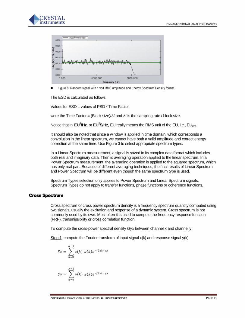
Figure 8. Random signal with 1 volt RMS amplitude and Energy Spectrum Density format.

The ESD is calculated as follows: Values for ESD = values of PSD * Time Factor were the Time Factor = (Block size)/∆f and ∆f is the sampling rate / block size. Notice that in

EU

2/Hz, or EU

2S/Hz, EU really means the RMS unit of the EU, i.e., EUrms.

It should also be noted that since a window is applied in time domain, which corresponds a convolution in the linear spectrum, we cannot have both a valid amplitude and correct energy correction at the same time. Use Figure 3 to select appropriate spectrum types. In a Linear Spectrum measurement, a signal is saved in its complex data format which includes both real and imaginary data. Then is averaging operation applied to the linear spectrum. In a Power Spectrum measurement, the averaging operation is applied to the squared spectrum, which has only real part. Because of different averaging techniques, the final results of Linear Spectrum and Power Spectrum will be different even though the same spectrum type is used. Spectrum Types selection only applies to Power Spectrum and Linear Spectrum signals. Spectrum Types do not apply to transfer functions, phase functions or coherence functions.

Cross Spectrum

Cross spectrum or cross power spectrum density is a frequency spectrum quantity computed using two signals, usually the excitation and response of a dynamic system. Cross spectrum is not commonly used by its own. Most often it is used to compute the frequency response function (FRF), transmissibility or cross correlation function. To compute the cross-power spectral density Gyx between channel x and channel y: Step 1, compute the Fourier transform of input signal x(k) and response signal y(k):

𝑆𝑥 = 𝑥 𝑘 𝑤 𝑘 𝑒−𝑗2𝜋𝑘𝑛 /𝑁

𝑁−1

𝑛=0

𝑆𝑦 = 𝑦 𝑘 𝑤 𝑘 𝑒−𝑗2𝜋𝑘𝑛 /𝑁

𝑁−1

𝑛=0



Step 2, compute the instantaneous cross power spectral density Syx = Sx

* Sy

T

Step 2, average the M frames of Sxx to get averaged PSD Gxx Gyx’ = Average (Syx) Step 3, Compute the energy correction and double the value for the single-sided spectra Gyx = 2 Gyx’ / EnergyCorr

Frequency Response and Coherence Function

The cross power spectrum method is often used for estimating the frequency response function (FRF) between channel x and channel y. The equation is:

𝐻𝑦𝑥 = 𝐺𝑦𝑥 / 𝐺𝑥𝑥

where Gyx is the averaged cross-spectrum between the input channel x and output channel y. Gxx is the averaged auto-spectrum of the input. Either power spectrum, power spectral density or energy spectral density can be used to compute the FRF because of the linear relationship between input and output. Using the cross-power spectrum method instead of simply dividing the linear spectra between input and output to calculate the FRF will reduce the effect of the noise at the output measurement end, as shown below.

Figure 9. Frequency response function computation.

The frequency response function has a complex data format. You can view it in real and imaginary or magnitude and phase display format. The coherence function is defined as:

yyxx

yx

yxGG

GC

2

2 ||

where Gyx is the averaged cross-spectrum between the input channel x and output channel y. Gxx and Gyy are the averaged auto-spectrum of the input and output. Either power spectrum, power spectral density or energy spectral density can be used here because of the linear relationship between input and output so that any multiplier factors will be cancelled out.



Coherence is a statistical measure of the how much of the output is caused by the input. The maximum coherence is 1.0 when the output is perfectly correlated with the input and zero when there is no correlation between input and output. Coherence is calculated by an average of multiple frames. When it is computed for only one frame, then the coherence function has a meaningless result of 1.0 due to the estimation error of the coherence function. The coherence function is a non-dimensional real function in the frequency domain. You can only view it in the real format.

Data Window Selection

Leakage Effect

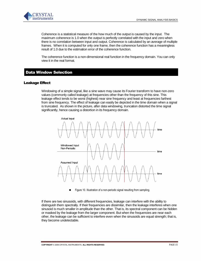
Windowing of a simple signal, like a sine wave may cause its Fourier transform to have non-zero values (commonly called leakage) at frequencies other than the frequency of this sine. This leakage effect tends to be worst (highest) near sine frequency and least at frequencies farthest from sine frequency. The effect of leakage can easily be depicted in the time domain when a signal is truncated. As shown in the picture, after data windowing, truncation distorted the time signal significantly, hence causing a distortion in its frequency domain.

Figure 10. Illustration of a non-periodic signal resulting from sampling.

If there are two sinusoids, with different frequencies, leakage can interfere with the ability to distinguish them spectrally. If their frequencies are dissimilar, then the leakage interferes when one sinusoid is much smaller in amplitude than the other. That is, its spectral component can be hidden or masked by the leakage from the larger component. But when the frequencies are near each other, the leakage can be sufficient to interfere even when the sinusoids are equal strength; that is, they become undetectable.



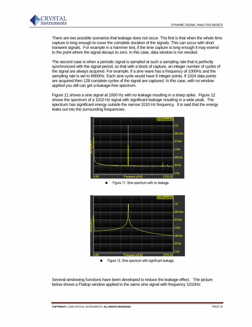
There are two possible scenarios that leakage does not occur. The first is that when the whole time capture is long enough to cover the complete duration of the signals. This can occur with short transient signals. For example in a hammer test, if the time capture is long enough it may extend to the point where the signal decays to zero. In this case, data window is not needed. The second case is when a periodic signal is sampled at such a sampling rate that is perfectly synchronized with the signal period, so that with a block of capture, an integer number of cycles of the signal are always acquired. For example, if a sine wave has a frequency of 1000Hz and the sampling rate is set to 8000Hz. Each sine cycle would have 8 integer points. If 1024 data points are acquired then 128 complete cycles of the signal are captured. In this case, with no window applied you still can get a leakage-free spectrum. Figure 11 shows a sine signal at 1000 Hz with no leakage resulting in a sharp spike. Figure 12 shows the spectrum of a 1010 Hz signal with significant leakage resulting in a wide peak. The spectrum has significant energy outside the narrow 1010 Hz frequency. It is said that the energy leaks out into the surrounding frequencies.

Figure 11. Sine spectrum with no leakage.

Figure 12. Sine spectrum with significant leakage.

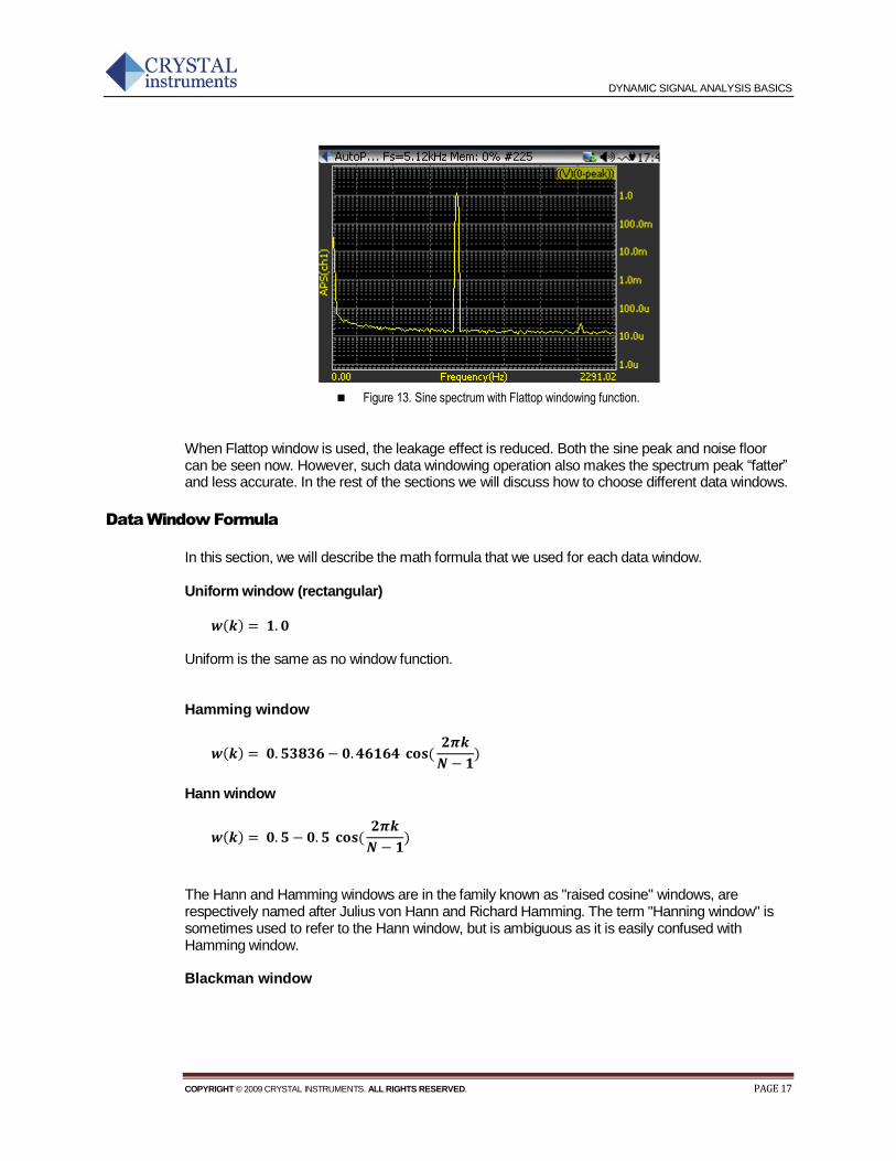
Several windowing functions have been developed to reduce the leakage effect. The picture below shows a Flattop window applied to the same sine signal with frequency 1010Hz:



Figure 13. Sine spectrum with Flattop windowing function.

When Flattop window is used, the leakage effect is reduced. Both the sine peak and noise floor can be seen now. However, such data windowing operation also makes the spectrum peak “fatter” and less accurate. In the rest of the sections we will discuss how to choose different data windows.

Data Window Formula

In this section, we will describe the math formula that we used for each data window.

Uniform window (rectangular)

𝒘 𝒌 = 𝟏. 𝟎 Uniform is the same as no window function. Hamming window

𝒘 𝒌 = 𝟎. 𝟓𝟑𝟖𝟑𝟔 − 𝟎. 𝟒𝟔𝟏𝟔𝟒 𝐜𝐨𝐬(𝟐𝝅𝒌

𝑵 − 𝟏)

Hann window

𝒘 𝒌 = 𝟎. 𝟓 − 𝟎. 𝟓 𝐜𝐨𝐬(𝟐𝝅𝒌

𝑵 − 𝟏)

The Hann and Hamming windows are in the family known as "raised cosine" windows, are respectively named after Julius von Hann and Richard Hamming. The term "Hanning window" is sometimes used to refer to the Hann window, but is ambiguous as it is easily confused with Hamming window. Blackman window



𝒘 𝒌 = 𝟎. 𝟖𝟒 − 𝟎. 𝟓 𝐜𝐨𝐬𝟐𝝅𝒌

𝑵 − 𝟏 + 𝟎. 𝟎𝟖𝐜𝐨𝐬

𝟒𝝅𝒌

𝑵 − 𝟏 𝒇𝒐𝒓 𝒌 = 𝟎~𝑵 − 𝟏

Flattop window

𝒘 𝒌 = 𝟏 − 𝟏. 𝟗𝟑𝐜𝐨𝐬𝟐𝝅𝒌

𝑵 − 𝟏 + 𝟏. 𝟐𝟗𝐜𝐨𝐬

𝟒𝝅𝒌

𝑵 − 𝟏− 𝟎. 𝟑𝟖𝟖𝐜𝐨𝐬

𝟔𝝅𝒌

𝑵 − 𝟏

+ 𝟎. 𝟎𝟑𝟐𝐜𝐨𝐬𝟖𝝅𝒌

𝑵 − 𝟏 𝒇𝒐𝒓 𝒌 = 𝟎~𝑵 − 𝟏

Kaiser Bessel window

𝒘 𝒌 = 𝟏. 𝟎 − 𝟏. 𝟐𝟒𝐜𝐨𝐬𝟐𝝅𝒌

𝑵 − 𝟏 + 𝟎. 𝟐𝟒𝟒𝐜𝐨𝐬

𝟒𝝅𝒌

𝑵 − 𝟏

+ 𝟎. 𝟎𝟎𝟑𝟎𝟓𝐜𝐨𝐬𝟔𝝅𝒌

𝑵 − 𝟏 𝒇𝒐𝒓 𝒌 = 𝟎~𝑵 − 𝟏

Exponential Window The shape of the exponential window is that of a decaying exponential. The following equation defines the exponential window.

𝒘 𝒌 = 𝒆 𝒌 𝐥𝐧(𝒇𝒊𝒏𝒂𝒍)

𝑵−𝟏

𝒇𝒐𝒓 𝒌 = 𝟎~𝑵 − 𝟏

where N is the length of the window, w(k)is the window value, and final is the final value of the whole sequence. The initial value of the window is one and gradually decays toward zero.

How to Choose the Right Data Window

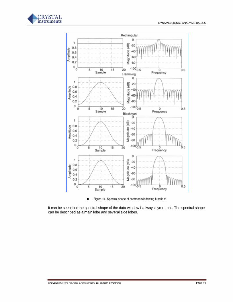
In this section we will discuss how to choose the data window. Figure 14 shows the spectral shape of four typical windows corresponding to their time waveform.



Figure 14. Spectral shape of common windowing functions.

It can be seen that the spectral shape of the data window is always symmetric. The spectral shape can be described as a main lobe and several side lobes.



-6dB

Main lobe width

Peak side

lobe level

Frequency

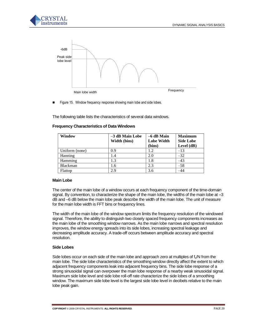
Figure 15. Window frequency response showing main lobe and side lobes.

The following table lists the characteristics of several data windows. Frequency Characteristics of Data Windows

Window –3 dB Main Lobe

Width (bins)

–6 dB Main

Lobe Width

(bins)

Maximum

Side Lobe

Level (dB)

Uniform (none) 0.9 1.2 –13

Hanning 1.4 2.0 –32

Hamming 1.3 1.8 –43

Blackman 1.6 2.3 –58

Flattop 2.9 3.6 –44

Main Lobe The center of the main lobe of a window occurs at each frequency component of the time-domain signal. By convention, to characterize the shape of the main lobe, the widths of the main lobe at –3 dB and –6 dB below the main lobe peak describe the width of the main lobe. The unit of measure for the main lobe width is FFT bins or frequency lines. The width of the main lobe of the window spectrum limits the frequency resolution of the windowed signal. Therefore, the ability to distinguish two closely spaced frequency components increases as the main lobe of the smoothing window narrows. As the main lobe narrows and spectral resolution improves, the window energy spreads into its side lobes, increasing spectral leakage and decreasing amplitude accuracy. A trade-off occurs between amplitude accuracy and spectral resolution. Side Lobes Side lobes occur on each side of the main lobe and approach zero at multiples of fs/N from the main lobe. The side lobe characteristics of the smoothing window directly affect the extent to which adjacent frequency components leak into adjacent frequency bins. The side lobe response of a strong sinusoidal signal can overpower the main lobe response of a nearby weak sinusoidal signal. Maximum side lobe level and side lobe roll-off rate characterize the side lobes of a smoothing window. The maximum side lobe level is the largest side lobe level in decibels relative to the main lobe peak gain.



Guidelines of Choosing Data Windows

If a measurement can be made so that no leakage effect will occur, then do not apply any window (in the software, select Uniform.). As discussed before, this only occurs when the time capture is long enough to cover the whole transient range, or when the signal is exactly periodic in the time frame. If the goal of the analysis is to discriminate two or multiple sine waves in the frequency domain, spectral resolution is very critical. For such application, choose a data window with very narrow main slope. Hanning is a good choice. If the goal of the analysis is to determine the amplitude reading of a periodic signal, i.e., to read EUpk, EUpkpk, EUrms or EUrms

2, the amplitude accuracy of a single frequency component is more

important than the exact location of the component in a given frequency bin, choose a window with a wide main lobe. Flattop window is often used. If you are analyzing transient signals such as impact and response signals, it is better not to use the spectral windows because these windows attenuate important information at the beginning of the sample block. Instead, use the Force and Exponential windows. A Force window is useful in analyzing shock stimuli because it removes stray signals at the end of the signal. The Exponential window is useful for analyzing transient response signals because it damps the end of the signal, ensuring that the signal fully decays by the end of the sample block. If the nature of the data is has a random nature or unknown, choose Hanning window.

Averaging Techniques

Averaging is widely used in spectral measurements. It improves the measurement and analysis of signals that are purely random or mixed random and periodic. Averaged measurements can yield either higher signal-to-noise ratios or improved statistical accuracy. Typically, three types of averaging methods are available in DSA products. They are: Linear Averaging, Exponential Averaging, and Peak-Hold

Linear Averaging

In linear averaging, each set of data (a record) contributes equally to the average. The value at any point in the linear average in given by the equation:

𝐴𝑣𝑒𝑟𝑎𝑔𝑒𝑑 = 𝑆𝑢𝑚 𝑜𝑓 𝑅𝑒𝑐𝑜𝑟𝑑𝑠

𝑁

N is the total number of the records. The advantage of this averaging method is that it is faster to compute and the result is un-biased. However, this method is suitable only for analyzing short signal records or stationary signals, since the average tends to stabilize. The contribution of new records eventually will cease to change the value of the average. Usually, a target average number is defined. The algorithm is made so that before the target average number reaches, the process can be stopped and the averaged result can still be used.



When the specified target averaging number is reached, the instrument usually will stop the acquisition and wait for the instruction for another collection of data acquisition.

Moving Linear Averaging

In a regular Linear Average, the data rate of the output of the averaging operator is only 1/N of that of the original signal. Therefore more averages takes longer to compute. Thus averaging will increase the time of the measurement. To reduce the time a Moving Linear Averaging can be used. Moving Linear Averaging uses overlapped input data points to generate more than 1/N results within a period of time. Moving linear average has the advantage that the resulted trace update time can be much shorter than the linear averaging period. Moving Linear Average is computed by

𝑦 𝑛 =1

𝑁 𝑥[𝑛 − 𝑗]

𝑁−1

𝑗 =0

Where x[k] is the input data, with sampling rate of T, y[n] is the output data, with Trace Update rate deltaT, AverageT is the period of Linear Average and ,N is the total samples used for Linear Average. N = AverageT/T

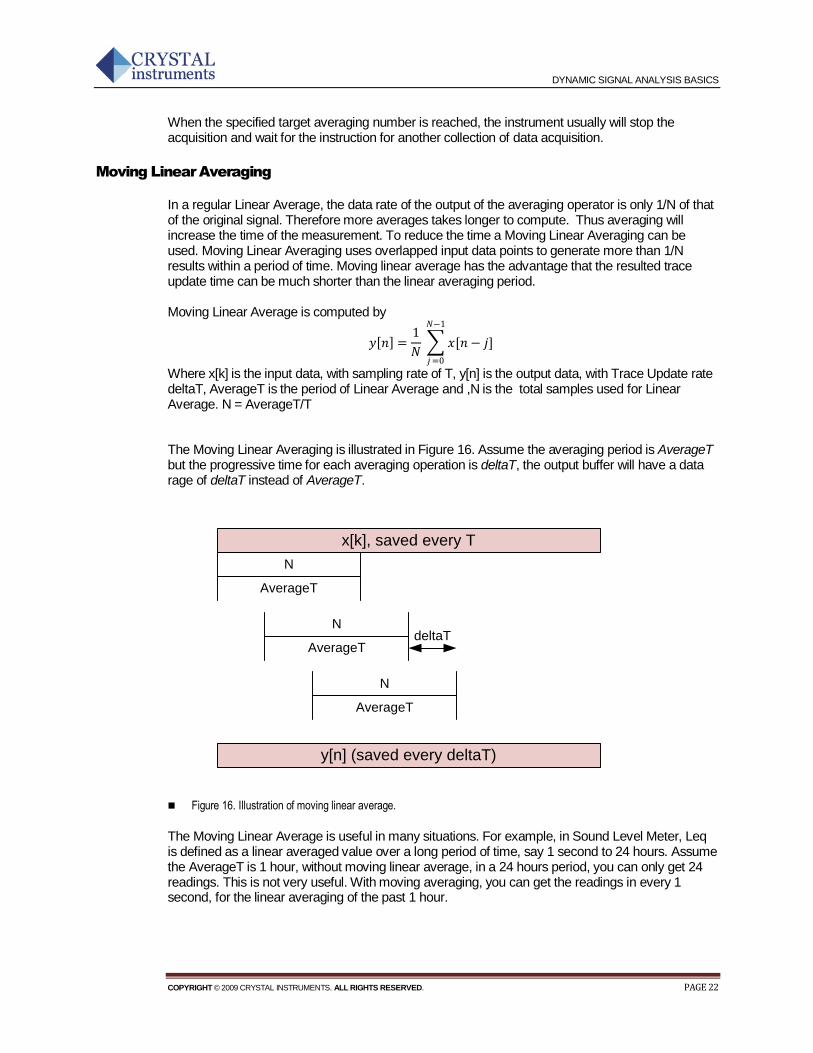
The Moving Linear Averaging is illustrated in Figure 16. Assume the averaging period is AverageT but the progressive time for each averaging operation is deltaT, the output buffer will have a data rage of deltaT instead of AverageT.

x[k], saved every T

AverageT

y[n] (saved every deltaT)

AverageT

AverageT

deltaT

N

N

N

Figure 16. Illustration of moving linear average.

The Moving Linear Average is useful in many situations. For example, in Sound Level Meter, Leq is defined as a linear averaged value over a long period of time, say 1 second to 24 hours. Assume the AverageT is 1 hour, without moving linear average, in a 24 hours period, you can only get 24 readings. This is not very useful. With moving averaging, you can get the readings in every 1 second, for the linear averaging of the past 1 hour.



Exponential Averaging

In exponential averaging, records do not contribute equally to the average. A new record is weighted more heavily than old ones. The value at any point in the exponential average is given by:

𝑦 𝑛 = 𝑦 𝑛 − 1 ∗ 1 − 𝛼 + 𝑥[𝑛] ∗ 𝛼

where 𝑦 𝑛 is the nth average and 𝑥[𝑛] is the nth new record. is the weighting coefficient. Usually

is defined as 1/(Number of Averaging). For example in the instrument, if the Number of Averaging is set to 3 and the averaging type is selected as exponential averaging, then 𝛼 = 1/3 The advantage of this averaging method is that it can be used indefinitely. That is, the average will not converge to some value and stay there, as is the case with linear averaging. The average will dynamically respond to the influence of new records and gradually ignore the effects of old records. Exponential averaging simulates the analog filter smoothing process. It will not reset when a specified averaging number is reached. The drawback of the exponential averaging is that a large value may embed too much memory into the average result. If there is a transient large value as input, it may take a long time for y[n] to decay. On the contrary, the contribution of small input value of x[n] will have little impact to the averaged output. Therefore, exponential average fits a stable signal better than a signal with large fluctuations.

Peak-Hold

This method, technically speaking, does not involve averaging in the strict sense of the word. Instead, the “average” produced by the peak hold method produces a record that at any point represents the maximum envelope among all the component records. The equation for a peak-hold is

𝑦 𝑛 = MAX j=0N−1 𝑥[𝑛 − 𝑗]

Peak-hold is useful for maintaining a record of the highest value attained at each point throughout the sequence of ensembles. Peak-Hold is not a linear math operation therefore it should be used carefully. It is acceptable to use Peak-Hold in auto-power spectrum measurement but you would not get meaningful results for FRF or Coherence measurement using Peak-Hold. Peak-hold averaging will reset after a specified averaging number is reached.

Linear Spectrum versus Power Spectrum Averaging

Averaging can be applied to either linear spectrum or power spectrum. If you want to reduce the spectral estimation variance, use power spectral averaging. If you want to extract repetitive or periodic small signals from a noisy signal, you can use triggered capture and average them in linear spectral domain. Linear Spectrum averaging must be performed with on a triggered event so that the time signal of one average is correlated with other similar measurements. Without time synchronizing mechanism, averaging in the Linear Spectrum domain makes no sense. Linear spectrum averaging is also called Vector averaging. It averages the complex FFT spectrum. (The



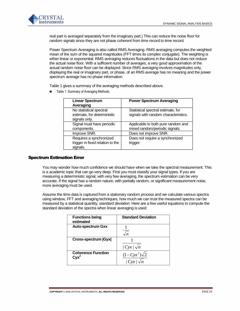
real part is averaged separately from the imaginary part.) This can reduce the noise floor for random signals since they are not phase coherent from time record to time record. Power Spectrum Averaging is also called RMS Averaging. RMS averaging computes the weighted mean of the sum of the squared magnitudes (FFT times its complex conjugate). The weighting is either linear or exponential. RMS averaging reduces fluctuations in the data but does not reduce the actual noise floor. With a sufficient number of averages, a very good approximation of the actual random noise floor can be displayed. Since RMS averaging involves magnitudes only, displaying the real or imaginary part, or phase, of an RMS average has no meaning and the power spectrum average has no phase information. Table 1 gives a summary of the averaging methods described above.

Table 1. Summary of Averaging Methods.

Linear Spectrum Averaging

Power Spectrum Averaging

No statistical spectral estimate, for deterministic signals only.

Statistical spectral estimate, for signals with random characteristics.

Signal must have periodic components.

Applicable to both pure random and mixed random/periodic signals.

Improve SNR. Does not improve SNR.

Requires a synchronized trigger in fixed relation to the signals.

Does not require a synchronized trigger.

Spectrum Estimation Error

You may wonder how much confidence we should have when we take the spectral measurement. This is a academic topic that can go very deep. First you must classify your signal types. If you are measuring a deterministic signal, with very few averaging, the spectrum estimation can be very accurate. If the signal has a random nature, with partially random, or significant measurement noise, more averaging must be used. Assume the time data is captured from a stationary random process and we calculate various spectra using window, FFT and averaging techniques, how much we can trust the measured spectra can be measured by a statistical quantity, standard deviation. Here are a few useful equations to compute the standard deviation of the spectra when linear averaging is used:

Functions being estimated

Standard Deviation

Auto-spectrum Gxx

n

1

Cross-spectrum |Gyx|

nCyx ||

1

Coherence Function Cyx

2

nCyx

Cyx

||

2)1( 2



Frequency Response Function Hyx

nCyx

Cyx

2||

)1( 2

where n is the average number in linear averaging. The transfer function is computed in the cross-power spectrum method as presented earlier. Assume a signal is random and has an expected power spectral density at 0.1 V

2/Hz. The goal of

a measurement is to average a few power spectra and to estimate such an expected value. If the average number is 1, meaning, with no average, the standard deviation of the error of such a measurement will be 100%. When we average two frames of auto power spectra, the standard

deviation of the error will become 1

2= 70.7% When the average number is increased to 100, the

standard deviation of the error of the reading is 10%. This means that the reading is likely in the neighborhood of (0.1±0.01) V

2/Hz

Now if this signal has a deterministic nature, say a sine wave, the spectral estimation error will only be applied to the random portion, i.e., the noisy portion, of this signal.

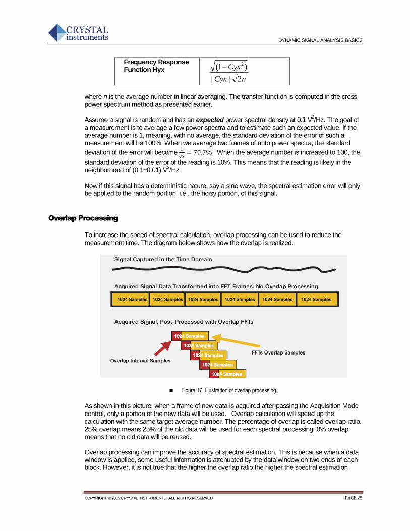
Overlap Processing

To increase the speed of spectral calculation, overlap processing can be used to reduce the measurement time. The diagram below shows how the overlap is realized.

Figure 17. Illustration of overlap processing.

As shown in this picture, when a frame of new data is acquired after passing the Acquisition Mode control, only a portion of the new data will be used. Overlap calculation will speed up the calculation with the same target average number. The percentage of overlap is called overlap ratio. 25% overlap means 25% of the old data will be used for each spectral processing. 0% overlap means that no old data will be reused. Overlap processing can improve the accuracy of spectral estimation. This is because when a data window is applied, some useful information is attenuated by the data window on two ends of each block. However, it is not true that the higher the overlap ratio the higher the spectral estimation



accuracy. For Hanning window, when the overlap ratio is more than 50%, the estimation accuracy of the spectra will not be improved. Another advantage to apply overlap processing is that it helps to update the display more quickly.

Single Degree of Freedom System

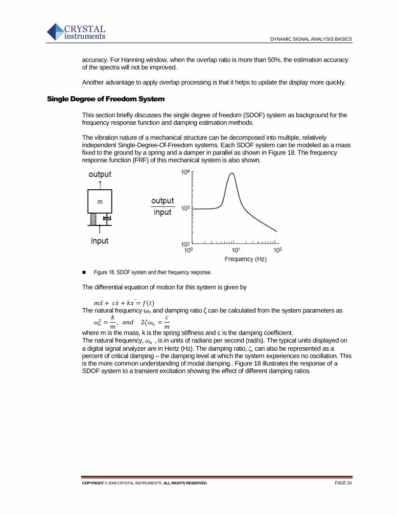
This section briefly discusses the single degree of freedom (SDOF) system as background for the frequency response function and damping estimation methods. The vibration nature of a mechanical structure can be decomposed into multiple, relatively independent Single-Degree-Of-Freedom systems. Each SDOF system can be modeled as a mass fixed to the ground by a spring and a damper in parallel as shown in Figure 18. The frequency response function (FRF) of this mechanical system is also shown.

Figure 18. SDOF system and their frequency response.

The differential equation of motion for this system is given by

𝑚𝑥 + 𝑐𝑥 + 𝑘𝑥 = 𝑓(𝑡) The natural frequency ωn and damping ratio ζ can be calculated from the system parameters as

𝜔𝑛2 =

𝑘

𝑚, 𝑎𝑛𝑑 2𝜁𝜔𝑛 =

𝑐

𝑚

where m is the mass, k is the spring stiffness and c is the damping coefficient. The natural frequency, 𝜔𝑛 , is in units of radians per second (rad/s). The typical units displayed on

a digital signal analyzer are in Hertz (Hz). The damping ratio, can also be represented as a percent of critical damping – the damping level at which the system experiences no oscillation. This is the more common understanding of modal damping.. Figure 18 illustrates the response of a SDOF system to a transient excitation showing the effect of different damping ratios.



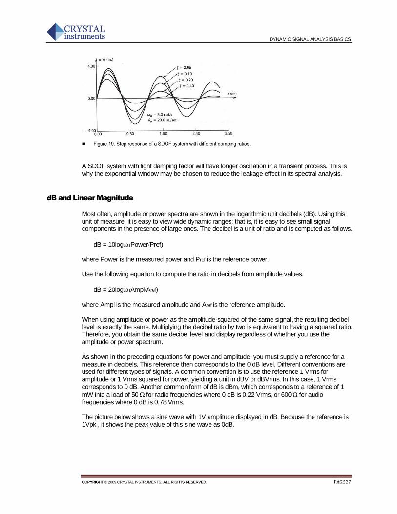
Figure 19. Step response of a SDOF system with different damping ratios.

A SDOF system with light damping factor will have longer oscillation in a transient process. This is why the exponential window may be chosen to reduce the leakage effect in its spectral analysis.

dB and Linear Magnitude

Most often, amplitude or power spectra are shown in the logarithmic unit decibels (dB). Using this unit of measure, it is easy to view wide dynamic ranges; that is, it is easy to see small signal components in the presence of large ones. The decibel is a unit of ratio and is computed as follows.

dB = 10log10 (PowerPref) where Power is the measured power and Pref is the reference power. Use the following equation to compute the ratio in decibels from amplitude values.

dB = 20log10 (AmplAref)

where Ampl is the measured amplitude and Aref is the reference amplitude. When using amplitude or power as the amplitude-squared of the same signal, the resulting decibel level is exactly the same. Multiplying the decibel ratio by two is equivalent to having a squared ratio. Therefore, you obtain the same decibel level and display regardless of whether you use the amplitude or power spectrum. As shown in the preceding equations for power and amplitude, you must supply a reference for a measure in decibels. This reference then corresponds to the 0 dB level. Different conventions are used for different types of signals. A common convention is to use the reference 1 Vrms for amplitude or 1 Vrms squared for power, yielding a unit in dBV or dBVrms. In this case, 1 Vrms corresponds to 0 dB. Another common form of dB is dBm, which corresponds to a reference of 1

mW into a load of 50 for radio frequencies where 0 dB is 0.22 Vrms, or 600 for audio frequencies where 0 dB is 0.78 Vrms. The picture below shows a sine wave with 1V amplitude displayed in dB. Because the reference is 1Vpk , it shows the peak value of this sine wave as 0dB.



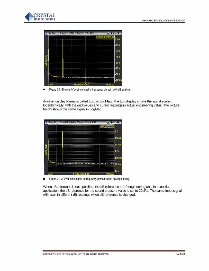
Figure 20. Show a 1Vpk sine signal in frequency domain with dB scaling.

Another display format is called Log, or LogMag. The Log display shows the signal scaled logarithmically with the grid values and cursor readings in actual engineering value. The picture below shows the same signal in LogMag.

Figure 21. A 1Vpk sine signal in frequency domain with LogMag scaling.

When dB reference is not specified, the dB reference is 1.0 engineering unit. In acoustics application, the dB reference for the sound pressure value is set to 20uPa. The same input signal will result in different dB readings when dB reference is changed.

8. TRANSIENT CAPURE AND HAMMER TESTING


TRANSIENT CAPTURE AND HAMMER TESTING

Transient Capture

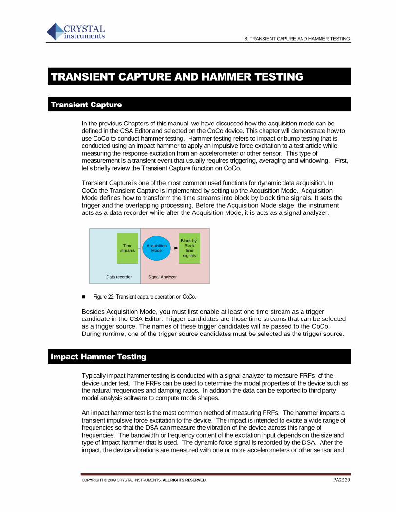
In the previous Chapters of this manual, we have discussed how the acquisition mode can be defined in the CSA Editor and selected on the CoCo device. This chapter will demonstrate how to use CoCo to conduct hammer testing. Hammer testing refers to impact or bump testing that is conducted using an impact hammer to apply an impulsive force excitation to a test article while measuring the response excitation from an accelerometer or other sensor. This type of measurement is a transient event that usually requires triggering, averaging and windowing. First, let’s briefly review the Transient Capture function on CoCo. Transient Capture is one of the most common used functions for dynamic data acquisition. In CoCo the Transient Capture is implemented by setting up the Acquisition Mode. Acquisition Mode defines how to transform the time streams into block by block time signals. It sets the trigger and the overlapping processing. Before the Acquisition Mode stage, the instrument acts as a data recorder while after the Acquisition Mode, it is acts as a signal analyzer.

Acquisition

Mode

Block-by-

Block

time

signals

Time

streams

Data recorder Signal Analyzer

Figure 22. Transient capture operation on CoCo.

Besides Acquisition Mode, you must first enable at least one time stream as a trigger candidate in the CSA Editor. Trigger candidates are those time streams that can be selected as a trigger source. The names of these trigger candidates will be passed to the CoCo. During runtime, one of the trigger source candidates must be selected as the trigger source.

Impact Hammer Testing

Typically impact hammer testing is conducted with a signal analyzer to measure FRFs of the device under test. The FRFs can be used to determine the modal properties of the device such as the natural frequencies and damping ratios. In addition the data can be exported to third party modal analysis software to compute mode shapes. An impact hammer test is the most common method of measuring FRFs. The hammer imparts a transient impulsive force excitation to the device. The impact is intended to excite a wide range of frequencies so that the DSA can measure the vibration of the device across this range of frequencies. The bandwidth or frequency content of the excitation input depends on the size and type of impact hammer that is used. The dynamic force signal is recorded by the DSA. After the impact, the device vibrations are measured with one or more accelerometers or other sensor and



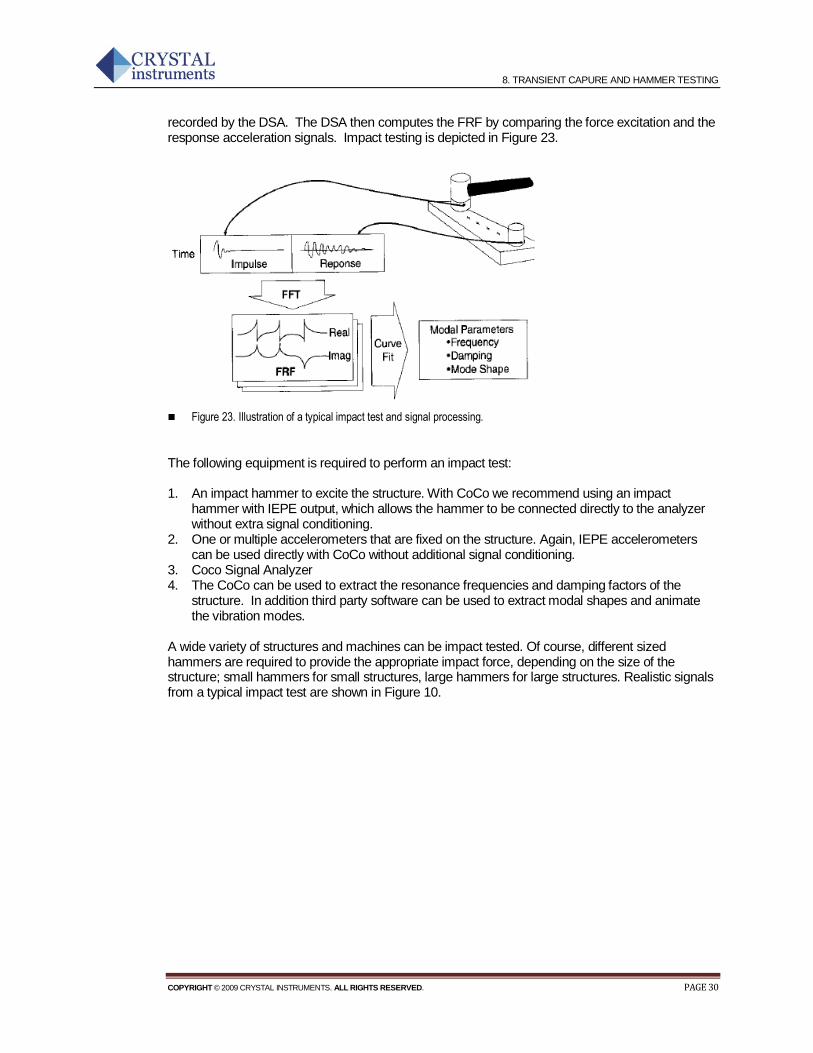
recorded by the DSA. The DSA then computes the FRF by comparing the force excitation and the response acceleration signals. Impact testing is depicted in Figure 23.

Figure 23. Illustration of a typical impact test and signal processing.

The following equipment is required to perform an impact test: 1. An impact hammer to excite the structure. With CoCo we recommend using an impact

hammer with IEPE output, which allows the hammer to be connected directly to the analyzer without extra signal conditioning.

2. One or multiple accelerometers that are fixed on the structure. Again, IEPE accelerometers can be used directly with CoCo without additional signal conditioning.

3. Coco Signal Analyzer 4. The CoCo can be used to extract the resonance frequencies and damping factors of the

structure. In addition third party software can be used to extract modal shapes and animate the vibration modes.

A wide variety of structures and machines can be impact tested. Of course, different sized hammers are required to provide the appropriate impact force, depending on the size of the structure; small hammers for small structures, large hammers for large structures. Realistic signals from a typical impact test are shown in Figure 10.



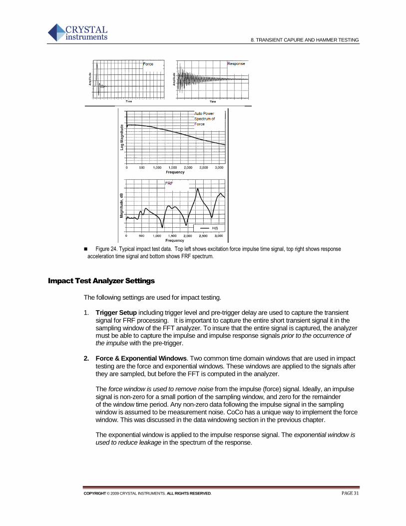
Figure 24. Typical impact test data. Top left shows excitation force impulse time signal, top right shows response

acceleration time signal and bottom shows FRF spectrum.

Impact Test Analyzer Settings

The following settings are used for impact testing. 1. Trigger Setup including trigger level and pre-trigger delay are used to capture the transient

signal for FRF processing. It is important to capture the entire short transient signal it in the sampling window of the FFT analyzer. To insure that the entire signal is captured, the analyzer must be able to capture the impulse and impulse response signals prior to the occurrence of the impulse with the pre-trigger.

2. Force & Exponential Windows. Two common time domain windows that are used in impact

testing are the force and exponential windows. These windows are applied to the signals after they are sampled, but before the FFT is computed in the analyzer.

The force window is used to remove noise from the impulse (force) signal. Ideally, an impulse signal is non-zero for a small portion of the sampling window, and zero for the remainder of the window time period. Any non-zero data following the impulse signal in the sampling window is assumed to be measurement noise. CoCo has a unique way to implement the force window. This was discussed in the data windowing section in the previous chapter. The exponential window is applied to the impulse response signal. The exponential window is used to reduce leakage in the spectrum of the response.



3. Accept/Reject: Because accurate impact testing results depend on the skill of the operator, FRF measurements should be made with averaging, a standard capability in all modern FFT analyzers. FRFs should be measured using at least 4 impacts per measurement. Since one or two of the impacts during the measurement process may be bad hits (too hard causing saturation, too soft causing poor coherence or a double hit causing distortion in the spectrum), an FFT analyzer designed for impact testing should have the ability to accept or reject the result of each impact after inspecting the impact signals. An accept/reject capability saves a lot of time during impact testing since you don’t have to redo all measurements in the averaging process after one bad hit.

4. Modal Damping Estimation. The width of the resonance peak is a measure of modal damping. The resonance peak width should also be the same for all FRF measurements, meaning that modal damping is the same in every FRF measurement. A good analyzer should provide an accurate damping factor estimate. CoCo uses a curve fitting algorithm to estimate the damping factor. The algorithm reduces the inaccuracy caused by the poor spectrum resolution or noise.

5. Modal Frequency estimation. The analyzer must provide capability of estimating the

resonance frequencies. CoCo uses an algorithm to identify the resonance frequencies based on the FRF.

References

To understand the topics of this article, we found the following three books to be very helpful:

1. Julius S. Bendat and Allan G. Piersol, Random Data, Analysis and Measurement Procedures, 2nd Edition, Wiley-Interscience, New York, 1986. 2. Julius S. Bendat and Allan G. Piesol, Engineering Applications of Correlation and Spectral Analysis, 2nd Edition, Wiley-Interscience, New York, 1993. 3. Sanjit K. Mitra and James F. Kaiser, Ed. Handbook for Digital Signal Processing, Wiley-Interscience, New York, 1993.

Documents

Dynamic Signal Analysis Basics - PROGRAMTEH Signal Analysis Basics.pdf · DYNAMIC SIGNAL ANALYSIS BASICS COPYRIGHT © 2009 CRYSTAL INSTRUMENTS.ALL RIGHTS RESERVED. PAGE 4 FREQUENCY