Bridge Engineering Handbook · Hydraulics 61.3 Bridge Scour Bridge Scour Analysis • Bridge Scour Calculation • Bridge Scour Investigation and Prevention 61.1 Introduction This

Springer, J., Zhou, K. "Bridge Hydraulics." Bridge Engineering Handbook. Ed. Wai-Fah Chen and Lian Duan Boca Raton: CRC Press, 2000

61Bridge Hydraulics

61.1 Introduction

61.2 Bridge Hydrology and HydraulicsHydrology • Bridge Deck Drainage Design • Stage Hydraulics

61.3 Bridge ScourBridge Scour Analysis • Bridge Scour Calculation • Bridge Scour Investigation and Prevention

61.1 Introduction

This chapter presents bridge engineers basic concepts, methods, and procedures used in bridgehydraulic analysis and design. It involves hydrology study, hydraulic analysis, on-site drainage design,and bridge scour evaluation.

Hydrology study for bridge design mainly deals with the properties, distribution, and circulationof water on and above the land surface. The primary objective is to determine either the peakdischarge or the flood hydrograph, in some cases both, at the highway stream crossings. Hydraulicanalysis provides essential methods to determine runoff discharges, water profiles, and velocitydistribution. The on-site drainage design part of this chapter is presented with the basic proceduresand references for bridge engineers to design bridge drainage.

Bridge scour is a big part of this chapter. Bridge engineers are systematically introduced toconcepts of various scour types, presented with procedures and methodology to calculate andevaluate bridge scour depths, provided with guidelines to conduct bridge scour investigation andto design scour preventive measures.

61.2 Bridge Hydrology and Hydraulics

61.2.1 Hydrology

61.2.1.1 Collection of DataHydraulic data for the hydrology study may be obtained from the following sources: as-built plans,site investigations and field surveys, bridge maintenance books, hydraulic files from experiencedreport writers, files of government agencies such as the U.S. Corps of Engineers studies, U.S.Geological Survey (USGS), Soil Conservation Service, and FEMA studies, rainfall data from localwater agencies, stream gauge data, USGS and state water agency reservoir regulation, aerial photo-graphs, and floodways, etc.

Site investigations should always be conducted except in the simplest cases. Field surveys are veryimportant because they can reveal conditions that are not readily apparent from maps, aerial

Jim SpringerCalifornia Department

of Transportation

Ke ZhouCalifornia Department

of Transportation

© 2000 by CRC Press LLC

photographs and previous studies. The typical data collected during a field survey include highwater marks, scour potential, stream stability, nearby drainage structures, changes in land use notindicated on maps, debris potential, and nearby physical features. See HEC-19, Attachment D [16]for a typical Survey Data Report Form.

61.2.1.2 Drainage BasinThe area of the drainage basin above a given point on a stream is a major contributing factor tothe amount of flow past that point. For given conditions, the peak flow at the proposed site isapproximately proportional to the drainage area.

The shape of a basin affects the peak discharge. Long, narrow basins generally give lower peakdischarges than pear-shaped basins. The slope of the basin is a major factor in the calculation ofthe time of concentration of a basin. Steep slopes tend to result in shorter times of concentrationand flatter slopes tend to increase the time of concentration. The mean elevation of a drainage basinis an important characteristic affecting runoff. Higher elevation basins can receive a significantamount of precipitation as snow. A basin orientation with respect to the direction of storm move-ment can affect peak discharge. Storms moving upstream tend to produce lower peaks than thosemoving downstream.

61.2.1.3 DischargeThere are several hydrologic methods to determine discharge. Most of the methods for estimatingflood flows are based on statistical analyses of rainfall and runoff records and involve preliminaryor trial selections of alternative designs that are judged to meet the site conditions and to accom-modate the flood flows selected for analysis.

Flood flow frequencies are usually calculated for discharges of 2.33 years through the overtoppingflood. The frequency flow of 2.33 years is considered to be the mean annual discharge. The baseflood is the 100-year discharge (1% frequency). The design discharge is the 50-year discharge (2%frequency) or the greatest of record, if practical. Many times, the historical flood is so large that astructure to handle the flow becomes uneconomical and is not warranted. It is the engineer’sresponsibility to determine the design discharge. The overtopping discharge is calculated at the site,but may overtop the roadway some distance away from the site.

Changes in land use can increase the surface water runoff. Future land-use changes that can bereasonably anticipated to occur in the design life should be used in the hydrology study. The typeof surface soil is a major factor in the peak discharge calculation. Rock formations underlying thesurface and other geophysical characteristics such as volcanic, glacial, and river deposits can havea significant effect on runoff. In the United States, the major source of soil information is the SoilConservation Service (SCS). Detention storage can have a significant effect on reducing the peakdischarge from a basin, depending upon its size and location in the basin.

The most commonly used methods to determine discharges are

1. Rational method2. Statistical Gauge Analysis Methods3. Discharge comparison of adjacent basins from gauge analysis4. Regional flood-frequency equations5. Design hydrograph

The results from various methods of determining discharge should be compared, not averaged.

61.2.1.3.1 Rational MethodThe rational method is one of the oldest flood calculation methods and was first employed in Irelandin urban engineering in 1847. This method is based on the following assumptions:


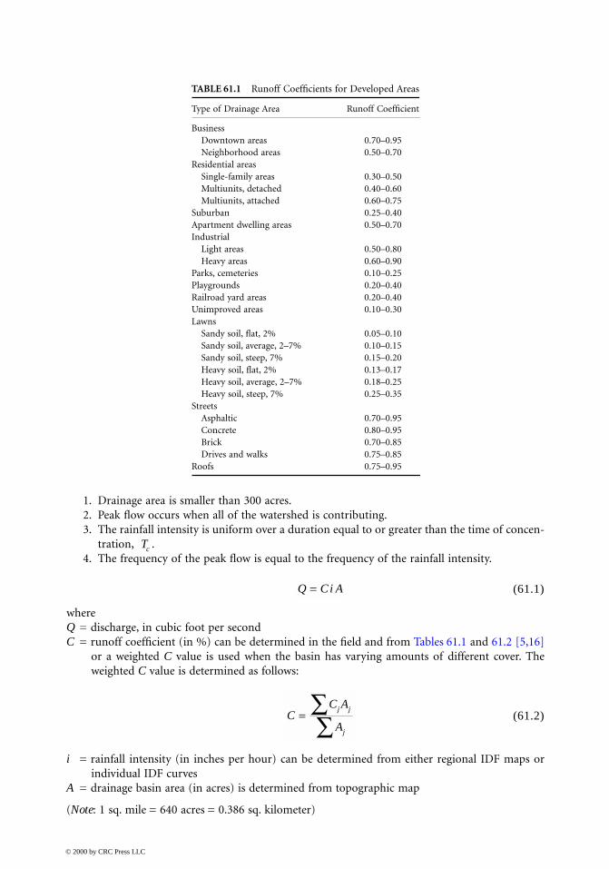
1. Drainage area is smaller than 300 acres.2. Peak flow occurs when all of the watershed is contributing.3. The rainfall intensity is uniform over a duration equal to or greater than the time of concen-

tration, .4. The frequency of the peak flow is equal to the frequency of the rainfall intensity.

(61.1)

whereQ = discharge, in cubic foot per secondC = runoff coefficient (in %) can be determined in the field and from Tables 61.1 and 61.2 [5,16]

or a weighted C value is used when the basin has varying amounts of different cover. Theweighted C value is determined as follows:

(61.2)

i = rainfall intensity (in inches per hour) can be determined from either regional IDF maps orindividual IDF curves

A = drainage basin area (in acres) is determined from topographic map

(Note: 1 sq. mile = 640 acres = 0.386 sq. kilometer)

TABLE 61.1 Runoff Coefficients for Developed Areas

Type of Drainage Area Runoff Coefficient

BusinessDowntown areas 0.70–0.95Neighborhood areas 0.50–0.70

Residential areasSingle-family areas 0.30–0.50Multiunits, detached 0.40–0.60Multiunits, attached 0.60–0.75

Suburban 0.25–0.40Apartment dwelling areas 0.50–0.70Industrial

Light areas 0.50–0.80Heavy areas 0.60–0.90

Parks, cemeteries 0.10–0.25Playgrounds 0.20–0.40Railroad yard areas 0.20–0.40Unimproved areas 0.10–0.30Lawns

Sandy soil, flat, 2% 0.05–0.10Sandy soil, average, 2–7% 0.10–0.15Sandy soil, steep, 7% 0.15–0.20Heavy soil, flat, 2% 0.13–0.17Heavy soil, average, 2–7% 0.18–0.25Heavy soil, steep, 7% 0.25–0.35

StreetsAsphaltic 0.70–0.95Concrete 0.80–0.95Brick 0.70–0.85Drives and walks 0.75–0.85

Roofs 0.75–0.95

Tc

Q Ci A=

CC A

A

j j

j

= ∑∑


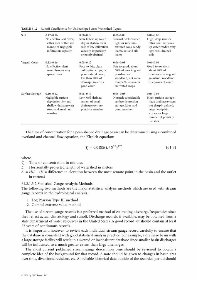
The time of concentration for a pear-shaped drainage basin can be determined using a combinedoverland and channel flow equation, the Kirpich equation:

(61.3)

where= Time of concentration in minutes

L = Horizontally projected length of watershed in metersS = H/L (H = difference in elevation between the most remote point in the basin and the outlet

in meters)

61.2.1.3.2 Statistical Gauge Analysis MethodsThe following two methods are the major statistical analysis methods which are used with streamgauge records in the hydrological analysis.

1. Log Pearson Type III method2. Gumbel extreme value method

The use of stream gauge records is a preferred method of estimating discharge/frequencies sincethey reflect actual climatology and runoff. Discharge records, if available, may be obtained from astate department of water resources in the United States. A good record set should contain at least25 years of continuous records.

It is important, however, to review each individual stream gauge record carefully to ensure thatthe database is consistent with good statistical analysis practice. For example, a drainage basin witha large storage facility will result in a skewed or inconsistent database since smaller basin dischargeswill be influenced to a much greater extent than large discharges.

The most current published stream gauge description page should be reviewed to obtain acomplete idea of the background for that record. A note should be given to changes in basin areaover time, diversions, revisions, etc. All reliable historical data outside of the recorded period should

TABLE 61.2 Runoff Coefficients for Undeveloped Area Watershed Types

Soil 0.12–0.16 0.08–0.12 0.06–0.08 0.04–0.06No effective soil cover,

either rock or thin soil mantle of negligible infiltration capacity

Slow to take up water, clay or shallow loam soils of low infiltration capacity, imperfectly or poorly drained

Normal, well-drained light or medium-textured soils, sandy loams, silt and silt loams

High, deep sand or other soil that takes up water readily, very light well-drained soils

Vegetal Cover 0.12–0.16 0.08–0.12 0.06–0.08 0.04–0.06No effective plant

cover, bare or very sparse cover

Poor to fair; clean cultivation crops, or poor natural cover, less than 20% of drainage area over good cover

Fair to good; about 50% of area in good grassland or woodland, not more than 50% of area in cultivated crops

Good to excellent; about 90% of drainage area in good grassland, woodland or equivalent cover

Surface Storage 0.10–0.12 0.08–0.10 0.06–0.08 0.04–0.06Negligible surface

depression few and shallow, drainageways steep and small, no marshes

Low, well-defined system of small drainageways; no ponds or marshes

Normal; considerable surface depression storage; lakes and pond marshes

High; surface storage, high; drainage system not sharply defined; large floodplain storage or large number of ponds or marshes

T L Sc = 0 0195 0 5 0 77. ( / ). .

Tc


be included. The adjacent gauge records for supplemental information should be checked andutilized to extend the record if it is possible. Natural runoff data should be separated from latercontrolled data. It is known that high-altitude basin snowmelt discharges are not compatible withrain flood discharges. The zero years must also be accounted for by adjusting the final plot positions,not by inclusion as minor flows. The generalized skew number can be obtained from the chart inBulletin No.17 B [8].

Quite often the database requires modification for use in a Log Pearson III analysis. Occasionally,a high outlier, but more often low outliers, will need to be removed from the database to avoidskewing results. This need is determined for high outliers by using = + K , and lowoutliers by using = + K , where K is a factor determined by the sample size, and

are the high and low mean logarithm of systematic peaks, and are the high and lowoutlier thresholds in log units, and are the high and low standard deviations of thelogarithmic distribution. Refer to FHWA HEC-19, Hydrology [16] or USGS Bulletin 17B [8] forthis method and to find the values of K.

The data to be plotted are “PEAK DISCHARGE, Q (CFS)” vs. “PROBABILITY, Pr” as shown inthe example in Figure 61.1. This plot usually results in a very flat curve with a reasonably straightcenter portion. An extension of this center portion gives a line for interpolation of the variousneeded discharges and frequencies.

The engineer should use an adjusted skew, which is calculated from the generalized and stationskews. Generalized skews should be developed from at least 40 stations with each station having atleast 25 years of record.

The equation for the adjusted skew is

(61.4)

where = weighted skew coefficient = station skew = generalized skew

= mean square error of station skew= mean square error of generalized skew

The entire Log Pearson type III procedure is covered by Bulletin No. 17B, “Guidelines for Deter-mining Flood Flow Frequency” [8].

The Gumbel extreme value method, sometimes called the double-exponential distribution ofextreme values, has also been used to describe the distribution of hydrological variables, especiallythe peak discharges. It is based on the assumption that the cumulative frequency distribution ofthe largest values of samples drawn from a large population can be described by the followingequation:

(61.5)

where

S = standard deviation= mean annual flow

QH QH

_SH

QL QL

_SL QH

_

QL

_QH QL

SH SL

GMSE G MSE G

MSE MSEwG L G S

G G

S L

S L

=++

( ) ( )

Gw

GS

GL

MSEGS

MSEGL

f Q e ea Q b

( )( )

= − −

aS

= 1 281.

b Q S= − 0 450.

Q


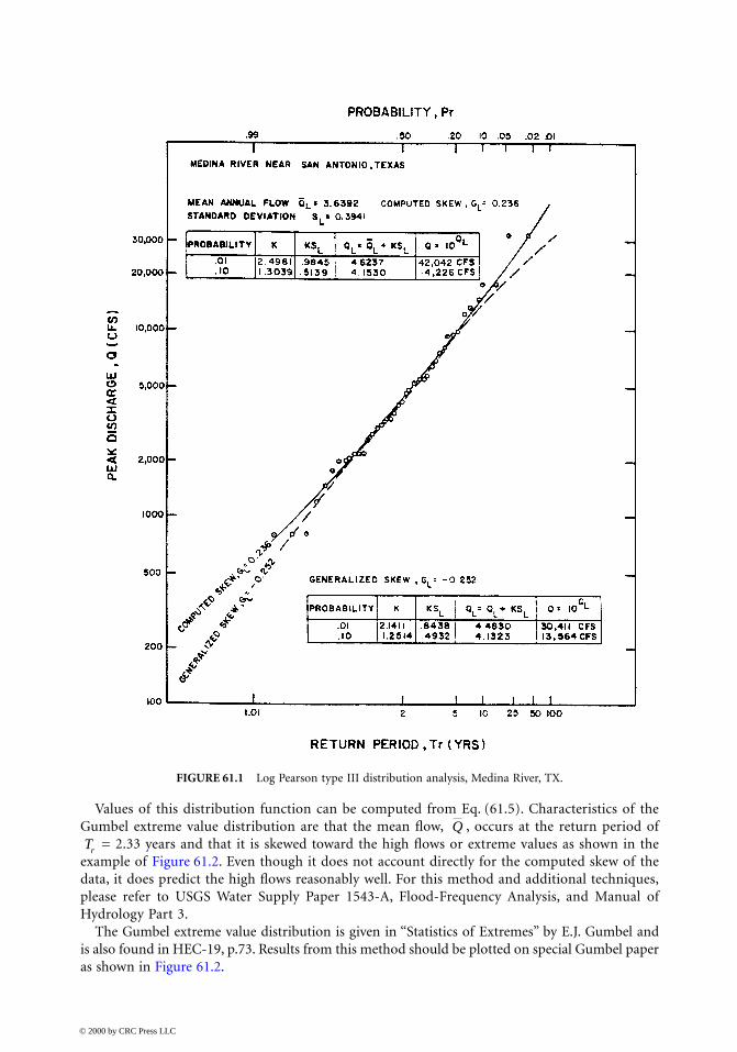
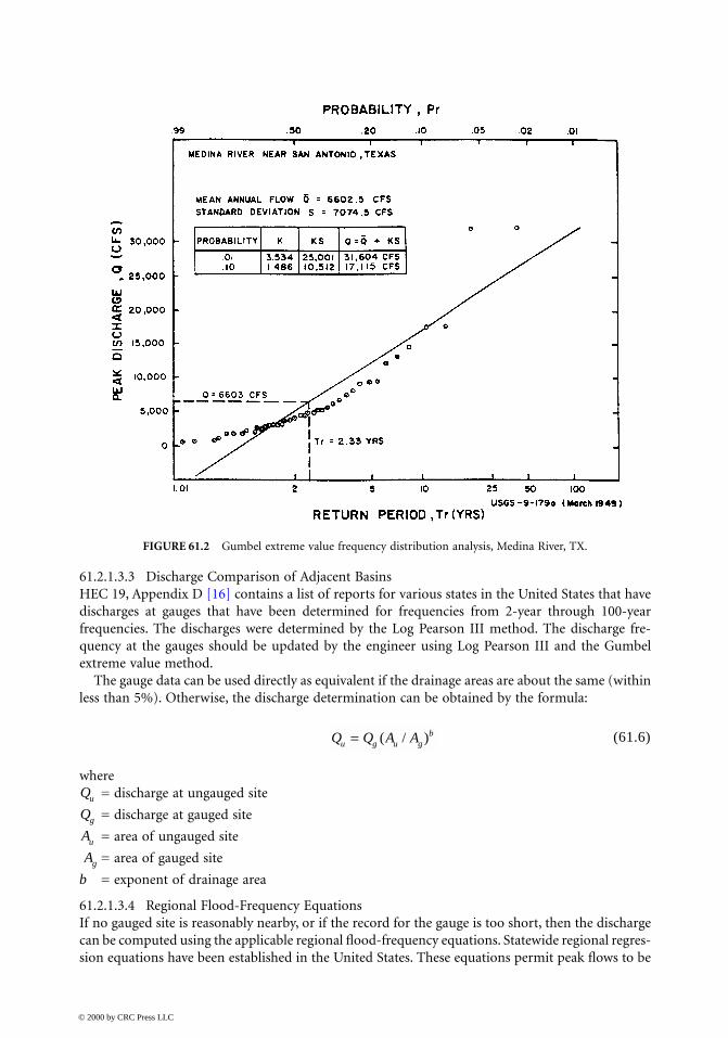
Values of this distribution function can be computed from Eq. (61.5). Characteristics of theGumbel extreme value distribution are that the mean flow, , occurs at the return period of

= 2.33 years and that it is skewed toward the high flows or extreme values as shown in theexample of Figure 61.2. Even though it does not account directly for the computed skew of thedata, it does predict the high flows reasonably well. For this method and additional techniques,please refer to USGS Water Supply Paper 1543-A, Flood-Frequency Analysis, and Manual ofHydrology Part 3.

The Gumbel extreme value distribution is given in “Statistics of Extremes” by E.J. Gumbel andis also found in HEC-19, p.73. Results from this method should be plotted on special Gumbel paperas shown in Figure 61.2.

FIGURE 61.1 Log Pearson type III distribution analysis, Medina River, TX.

QTr


61.2.1.3.3 Discharge Comparison of Adjacent BasinsHEC 19, Appendix D [16] contains a list of reports for various states in the United States that havedischarges at gauges that have been determined for frequencies from 2-year through 100-yearfrequencies. The discharges were determined by the Log Pearson III method. The discharge fre-quency at the gauges should be updated by the engineer using Log Pearson III and the Gumbelextreme value method.

The gauge data can be used directly as equivalent if the drainage areas are about the same (withinless than 5%). Otherwise, the discharge determination can be obtained by the formula:

(61.6)

where= discharge at ungauged site

= discharge at gauged site

= area of ungauged site

= area of gauged site

b = exponent of drainage area

61.2.1.3.4 Regional Flood-Frequency EquationsIf no gauged site is reasonably nearby, or if the record for the gauge is too short, then the dischargecan be computed using the applicable regional flood-frequency equations. Statewide regional regres-sion equations have been established in the United States. These equations permit peak flows to be

FIGURE 61.2 Gumbel extreme value frequency distribution analysis, Medina River, TX.

Q Q A Au g u gb= ( / )

Qu

Qg

Au

Ag


estimated for return periods varying between 2 and 100 years. The discharges were determined bythe Log Pearson III method. See HEC-19, Appendix D [16] for references to the studies that wereconducted for the various states.

61.2.1.3.5 Design HydrographsDesign hydrographs [9] give a complete time history of the passage of a flood at a particular site.This would include the peak flow. A runoff hydrograph is a plot of the response of a watershed toa particular rainfall event. A unit hydrograph is defined as the direct runoff hydrograph resultingfrom a rainfall event that lasts for a unit duration of time. The ordinates of the unit hydrographare such that the volume of direct runoff represented by the area under the hydrograph is equal to1 in. of runoff from the drainage area. Data on low water discharges and dates should be given asit will control methods and procedures of pier excavation and construction. The low water dischargesand dates can be found in the USGS Water Resources Data Reports published each year. Oneprocedure is to review the past 5 or 6 years of records to determine this.

61.2.1.4 RemarksBefore arriving at a final discharge, the existing channel capacity should be checked using the velocityas calculated times the channel waterway area. It may be that a portion of the discharge overflowsthe banks and never reaches the site.

The proposed design discharge should also be checked to see that it is reasonable and practicable.As a rule of thumb, the unit runoff should be 300 to 600 s-ft per square mile for small basins (to20 square miles), 100 to 300 s-ft per square mile for median areas (to 50 square miles) and 25 to150 s-ft for large basins (above 50 square miles). The best results will depend on rational engineeringjudgment.

61.2.2 Bridge Deck Drainage Design (On-Site Drainage Design)

61.2.2.1 Runoff and Capacity AnalysisThe preferred on-site hydrology method is the rational method. The rational method, as discussedin Section 61.2.1.3.1, for on-site hydrology has a minimum time of concentration of 10 min. Manytimes, the time of concentration for the contributing on-site pavement runoff is less than 10 min.The initial time of concentration can be determined using an overland flow method until the runoffis concentrated in a curbed section. Channel flow using the roadway-curb cross section should beused to determine velocity and subsequently the time of flow to the first inlet. The channel flowvelocity and flooded width is calculated using Manning’s formula:

(61.7)

whereV = velocityA = cross-sectional area of flowR = hydraulic radius

= slope of channeln = Manning’s roughness value [11]

The intercepted flow is subtracted from the initial flow and the bypass is combined with runofffrom the subsequent drainage area to determine the placement of the next inlet. The placement ofinlets is determined by the allowable flooded width on the roadway.

Oftentimes, bridges are in sump areas, or the lowest spot on the roadway profile. This necessitatesthe interception of most of the flow before reaching the bridge deck. Two overland flow equationsare as follows.

Vn

A R Sf= 1 486 2 3 1 2. / /

Sf


1. Kinematic Wave Equation:

(61.8)

2. Overland Equation:

(61.9)

where= overland flow travel time in minutes

L = length of overland flow path in metersS = slope of overland flow in metersn = manning’s roughness coefficient [12]i = design storm rainfall intensity in mm/hC = runoff coefficient (Tables 61.1 and 61.2)

61.2.2.2 Select and Size Drainage FacilitiesThe selection of inlets is based upon the allowable flooded width. The allowable flooded width isusually outside the traveled way. The type of inlet leading up to the bridge deck can vary dependingupon the flooded width and the velocity. Grate inlets are very common and, in areas with curbs,curb opening inlets are another alternative. There are various monographs associated with the typeof grate and curb opening inlet. These monographs are used to determine interception and thereforethe bypass [5].

61.2.3 Stage Hydraulics

High water (HW) stage is a very important item in the control of the bridge design. All availableinformation should be obtained from the field and the Bridge Hydrology Report regarding HWmarks, HW on upstream and downstream sides of the existing bridges, high drift profiles, andpossible backwater due to existing or proposed construction.

Remember, observed high drift and HW marks are not always what they seem. Drift in trees andbrush that could have been bent down by the flow of the water will be extremely higher than theactual conditions. In addition, drift may be pushed up on objects or slopes above actual HWelevation by the velocity of the water or wave action. Painted HW marks on the bridge should besearched carefully. Some flood insurance rate maps and flood insurance study reports may showstages for various discharges. Backwater stages caused by other structures should be included orstreams should be noted.

Duration of high stages should be given, along with the base flood stage and HW for the designdischarge. It should be calculated for existing and proposed conditions that may restrict the channelproducing a higher stage. Elevation and season of low water should be given, as this may controldesign of tremie seals for foundations and other possible methods of construction. Elevation ofovertopping flow and its location should be given. Normally, overtopping occurs at the bridge site,but overtopping may occur at a low sag in the roadway away from the bridge site.

61.2.3.1 Waterway AnalysisWhen determining the required waterway at the proposed bridge, the engineers must consider alladjacent bridges if these bridges are reasonably close. The waterway section of these bridges shouldbe tied into the stream profile of the proposed structure. Structures that are upstream or downstreamof the proposed bridge may have an impact on the water surface profile. When calculating the

tL n

i So = 6 92 0 6 0 6

0 4 0 3

. . .

. .

tC LSo = −3 3 1 1

100

1 2

1 3

. ( . )( )( )

/

/

to


effective waterway area, adjustments must be made for the skew and piers and bents. The requiredwaterway should be below the 50-year design HW stage.

If stream velocities, scour, and erosive forces are high, then abutments with wingwall constructionmay be necessary. Drift will affect the horizontal clearance and the minimum vertical clearance lineof the proposed structure. Field surveys should note the size and type of drift found in the channel.Designs based on the 50-year design discharge will require drift clearance. On major streams andrivers, drift clearance of 2 to 5 m above the 50-year discharge is needed. On smaller streams 0.3 to1 m may be adequate. A formula for calculating freeboard is

Freeboard (61.10)

whereQ = dischargeV = velocity

61.2.3.2 Water Surface Profile CalculationThere are three prominent water surface profile calculation programs available [1,2]. The firstone is HEC-2 which takes stream cross sections perpendicular to the flow. WSPRO is similar toHEC-2 with some improvements. SMS is a new program that uses finite-element analysis for itscalculations. SMS can utilize digital elevation models to represent the streambeds.

61.2.2.3 Flow Velocity and DistributionMean channel, overflow velocities at peak stage, and localized velocity at obstructions such as piersshould be calculated or estimated for anticipated high stages. Mean velocities may be calculatedfrom known stream discharges at known channel section areas or known waterway areas of bridge,using the correct high water stage.

Surface water velocities should be measured roughly, by use of floats, during field surveys forsites where the stream is flowing. Stream velocities may be calculated along a uniform section ofthe channel using Manning’s formula Eq. (61.7) if the slope, channel section (area and wettedperimeter), and roughness coefficient (n) are known.

At least three profiles should be obtained, when surveying for the channel slope, if possible. Thesethree slopes are bottom of the channel, the existing water surface, and the HW surface based ondrift or HW marks. The top of low bank, if overflow is allowed, should also be obtained. In addition,note some tops of high banks to prove flows fall within the channel. These profiles should be plottedshowing existing and proposed bridges or other obstruction in the channel, the change of HW slopedue to these obstructions and possible backwater slopes.

The channel section used in calculating stream velocities should be typical for a relatively longsection of uniform channel. Since this theoretical condition is not always available, however, thenearest to uniform conditions should be used with any necessary adjustments made for irregularities.

Velocities may be calculated from PC programs, or calculator programs, if the hydraulic radius,roughness factor, and slope of the channel are known for a section of channel, either natural orartificial, where uniform stream flow conditions exists. The hydraulic radius is the waterway areadivided by the wetted perimeter of an average section of the uniform channel. A section under abridge whose piers, abutments, or approach fills obstruct the uniformity of the channel cannot beused as there will not be uniform flow under the structure. If no part of the bridge structure seriouslyobstructs or restricts the channel, however, the section at the bridge could be used in the aboveuniform flow calculations.

The roughness coefficient n for the channel will vary along the length of the channel for variouslocations and conditions. Various values for n can be found in the References [1,5,12,17].

At the time of a field survey the party chief should estimate the value of n to be used for thechannel section under consideration. Experience is required for field determination of a relatively

= +0 1 0 0080 3 2. ..Q V


close to actual n value. In general, values for natural streams will vary between 0.030 and 0.070.Consider both low and HW n value. The water surface slope should be used in this plot and theslope should be adjusted for obstructions such as bridges, check dams, falls, turbulence, etc.

The results as obtained from this plot may be inaccurate unless considerable thought is given tothe various values of slope, hydraulic radius, and n. High velocities between 15 and 20 ft/s (4.57and 6.10 m/s through a bridge opening may be undesirable and may require special design consid-erations. Velocities over 20/ 6.10 m/s should not be used unless special design features are incor-porated or if the stream is mostly confined in rock or an artificial channel.

61.3 Bridge Scour

61.3.1 Bridge Scour Analysis

61.3.1.1 Basic Scour ConceptsScour is the result of the erosive action of flowing water, excavating and carrying away materialfrom the bed and banks of streams. Determining the magnitude of scour is complicated by thecyclic nature of the scour process. Designers and inspectors need to study site-specific subsurfaceinformation carefully in evaluating scour potential at bridges. In this section, we present bridgeengineers with the basic procedures and methods to analyze scour at bridges.

Scour should be investigated closely in the field when designing a bridge. The designer usuallyplaces the top of footings at or below the total potential scour depth; therefore, determining thedepth of scour is very important. The total potential scour at a highway crossing usually comprisesthe following components [11]: aggradation and degradation, stream contraction scour, local scour,and sometimes with lateral stream migration.

61.3.1.1.1 Long-Term Aggradation and DegradationWhen natural or human activities cause streambed elevation changes over a long period of time,aggradation or degradation occurs. Aggradation involves the deposition of material eroded fromthe channel or watershed upstream of the bridge, whereas degradation involves the lowering orscouring of the streambed due to a deficit in sediment supply from upstream.

Long-term streambed elevation changes may be caused by the changing natural trend of thestream or may be the result of some anthropogenic modification to the stream or watershed. Factorsthat affect long-term bed elevation changes are dams and reservoirs up- or downstream of thebridge, changes in watershed land use, channelization, cutoffs of meandering river bends, changesin the downstream channel base level, gravel mining from the streambed, diversion of water into orout of the stream, natural lowering of the fluvial system, movement of a bend, bridge location withrespect to stream planform, and stream movement in relation to the crossing. Tidal ebb and flood maydegrade a coastal stream, whereas littoral drift may cause aggradation. The problem for the bridgeengineer is to estimate the long-term bed elevation changes that will occur during the lifetime of thebridge.

61.3.1.1.2 Stream Contraction ScourContraction scour usually occurs when the flow area of a stream at flood stage is reduced, eitherby a natural contraction or an anthropogenic contraction (like a bridge). It can also be caused bythe overbank flow which is forced back by structural embankments at the approaches to a bridge.There are some other causes that can lead to a contraction scour at a bridge crossing [11]. Thedecreased flow area causes an increase in average velocity in the stream and bed shear stress throughthe contraction reach. This in turn triggers an increase in erosive forces in the contraction. Hence,more bed material is removed from the contracted reach than is transported into the reach. Thenatural streambed elevation is lowered by this contraction phenomenon until relative equilibriumis reached in the contracted stream reach.


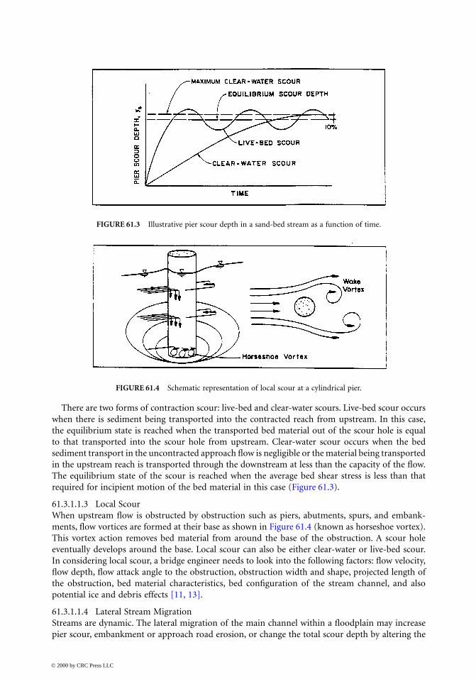
There are two forms of contraction scour: live-bed and clear-water scours. Live-bed scour occurswhen there is sediment being transported into the contracted reach from upstream. In this case,the equilibrium state is reached when the transported bed material out of the scour hole is equalto that transported into the scour hole from upstream. Clear-water scour occurs when the bedsediment transport in the uncontracted approach flow is negligible or the material being transportedin the upstream reach is transported through the downstream at less than the capacity of the flow.The equilibrium state of the scour is reached when the average bed shear stress is less than thatrequired for incipient motion of the bed material in this case (Figure 61.3).

61.3.1.1.3 Local ScourWhen upstream flow is obstructed by obstruction such as piers, abutments, spurs, and embank-ments, flow vortices are formed at their base as shown in Figure 61.4 (known as horseshoe vortex).This vortex action removes bed material from around the base of the obstruction. A scour holeeventually develops around the base. Local scour can also be either clear-water or live-bed scour.In considering local scour, a bridge engineer needs to look into the following factors: flow velocity,flow depth, flow attack angle to the obstruction, obstruction width and shape, projected length ofthe obstruction, bed material characteristics, bed configuration of the stream channel, and alsopotential ice and debris effects [11, 13].

61.3.1.1.4 Lateral Stream MigrationStreams are dynamic. The lateral migration of the main channel within a floodplain may increasepier scour, embankment or approach road erosion, or change the total scour depth by altering the

FIGURE 61.3 Illustrative pier scour depth in a sand-bed stream as a function of time.

FIGURE 61.4 Schematic representation of local scour at a cylindrical pier.


flow angle of attack at piers. Lateral stream movements are affected mainly by the geomorphologyof the stream, location of the crossing on the stream, flood characteristics, and the characteristicsof the bed and bank materials [11,13].

61.3.1.2 Designing Bridges to Resist ScourIt is obvious that all scour problems cannot be covered in this special topic section of bridge scour.A more-detailed study can be found in HEC-18, “Evaluating Scour at Bridges” and HEC-20, “StreamStability at Highway Structures” [11,18]. As described above, the three most important componentsof bridge scour are long-term aggradation or degradation, contraction scour, and local scour. Thetotal potential scour is a combination of the three components. To design a bridge to resist scour,a bridge engineer needs to follow the following observation and investigation steps in the designprocess.

1. Field Observation — Main purposes of field observation are as follows:

• Observe conditions around piers, columns, and abutments (Is the hydraulic skew correct?),

• Observe scour holes at bends in the stream,

• Determine streambed material,

• Estimate depth of scour, and

• Complete geomorphic factor analysis.

There is usually no fail-safe method to protect bridges from scour except possibly keepingpiers and abutments out of the HW area; however, proper hydraulic bridge design canminimize bridge scour and its potential negative impacts.

2. Historic Scour Investigation — Structures that have experienced scour in the past are likelyto continue displaying scour problems in the future. The bridges that we are most concernedwith include those currently experiencing scour problems and exhibiting a history of localscour problems.

3. Problem Location Investigation — Problem locations include “unsteady stream” locations,such as near the confluence of two streams, at the crossing of stream bends, and at alluvialfan deposits.

4. Problem Stream Investigation — Problem streams are those that have the following char-acteristics of aggressive tendencies: indication of active degradation or aggradation; migrationof the stream or lateral channel movement; streams with a steep lateral slope and/or highvelocity; current, past, or potential in-stream aggregate mining operations; and loss of bankprotection in the areas adjacent to the structure.

5. Design Feature Considerations — The following features, which increase the susceptibilityto local scour, should be considered:

• Inadequate waterway opening leads to inadequate clearance to pass large drift during heavyrunoff.

• Debris/drift problem: Light drift or debris may cause significant scour problems, moderatedrift or debris may cause significant scour but will not create severe lateral forces on thestructure, and heavy drift can cause strong lateral forces or impact damage as well as severescour.

• Lack of overtopping relief: Water may rise above deck level. This may not cause scourproblems but does increase vulnerability to severe damage from impact by heavy drift.

• Incorrect pier skew: When the bridge pier does not match the channel alignment, it maycause scour at bridge piers and abutments.

6. Traffic Considerations — The amount of traffic such as average daily traffic (ADT), type oftraffic, the length of detour, the importance of crossings, and availability of other crossingsshould be taken into consideration.


7. Potential for Unacceptable Damage — Potential for collapse during flood, safety of travelingpublic and neighbors, effect on regional transportation system, and safety of other facilities(other bridges, properties) need to be evaluated.

8. Susceptibility of Combined Hazard of Scour and Seismic — The earthquake prioritizationlist and the scour-critical list are usually combined for bridge design use.

61.3.1.3 Scour RatingIn the engineering practice of the California Department of Transportation, the rating of eachstructure is based upon the following:

1. Letter grading — The letter grade is related to the potential for scour-related problems atthis location.

2. Numerical grading — The numerical rating associated with each structure is a determinationof the severity for the potential scour:

A-1 No problem anticipatedA-2 No problem anticipated/new bridge — no historyA-3 Very remote possibility of problemsB-1 Slight possibility of problemsB-2 Moderate possibility of problemsB-3 Strong possibility of problemsC-1 Some probability of problemsC-2 Moderate probability of problemsC-3 Very strong probability of problems

Scour effect of storms is usually greater than design frequency, say, 500-year frequency. FHWAspecifies 500-year frequency as 1.7 times 100-year frequency. Most calculations indicate 500-yearfrequency is 1.25 to 1.33 times greater than the 100-year frequency [3,8]; the 1.7 multiplier shouldbe a maximum. Consider the amount of scour that would occur at overtopping stages and alsopressure flows. Be aware that storms of lesser frequency may cause larger scour stress on the bridge.

61.3.2 Bridge Scour Calculation

All the equations for estimating contraction and local scour are based on laboratory experimentswith limited field verification [11]. However, the equations recommended in this section are con-sidered to be the most applicable for estimating scour depths. Designers also need to give differentconsiderations to clear-water scour and live-bed scour at highway crossings and encroachments.

Prior to applying the bridge scour estimating methods, it is necessary to (1) obtain the fixed-bedchannel hydraulics, (2) determine the long-term impact of degradation or aggradation on the bedprofile, (3) adjust the fixed-bed hydraulics to reflect either degradation or aggradation impact, and(4) compute the bridge hydraulics accordingly.

61.3.2.1 Specific Design ApproachFollowing are the recommended steps for determining scour depth at bridges:

Step 1: Analyze long-term bed elevation change.Step 2: Compute the magnitude of contraction scour.Step 3: Compute the magnitude of local scour at abutments.Step 4: Compute the magnitude of local scour at piers.Step 5: Estimate and evaluate the total potential scour depths.

The bridge engineers should evaluate if the individual estimates of contraction and local scourdepths from Step 2 to 4 are reasonable and evaluate the total scour derived from Step 5.


61.3.2.2 Detailed Procedures

1. Analyze Long-Term Bed Elevation Change — The face of bridge sections showing bedelevation are available in the maintenance bridge books, old preliminary reports, and some-times in FEMA studies and U.S. Corps of Engineers studies. Use this information to estimateaggradation or degradation.

2. Compute the Magnitude of Contraction Scour — It is best to keep the bridge out of thenormal channel width. However, if any of the following conditions are present, calculatecontraction scour.a. Structure over channel in floodplain where the flows are forced through the structure due

to bridge approachesb. Structure over channel where river width becomes narrowc. Relief structure in overbank area with little or no bed material transportd. Relief structure in overbank area with bed material transportThe general equation for determining contraction scour is

(61.11)

where= depth of scour= average water depth in the main channel= average water depth in the contracted section

Other contraction scour formulas are given in the November 1995 HEC-18 publication —also refer to the workbook or HEC-18 for the various conditions listed above [11]. Thedetailed scour calculation procedures can be referenced from this circular for either live-bedor clear-water contraction scour.

3. Compute the Magnitude of Local Scour at Abutments — Again, it is best to keep theabutments out of the main channel flow. Refer to publication HEC-18 from FHWA [13]. Thescour formulas in the publication tend to give excessive scour depths.

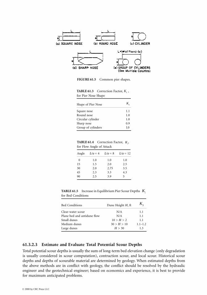
4. Compute the Magnitude of Local Scour at Piers — The pier alignment is the most criticalfactor in determining scour depth. Piers should align with stream flow. When flow directionchanges with stages, cylindrical piers or some variation may be the best alternative. Becautious, since large-diameter cylindrical piers can cause considerable scour. Pier width andpier nose are also critical elements in causing excessive scour depth.

Assuming a sand bed channel, an acceptable method to determine the maximum possible scourdepth for both live-bed and clear-water channel proposed by the Colorado State University [11] isas follows:

(61.12)

where= scour depth= flow depth just upstream of the pier= correction for pier shape from Figure 61.5 and Table 61.3= correction for angle of attack of flow from Table 61.4= correction for bed condition from Table 61.5

a = pier widthl = pier length

= Froude number = (just upstream from bridge)

Drift retention should be considered when calculating pier width/type.

y y ys = −2 1

ys

y1

y2

y

yK K K

ay

F lsr

11 2 3

1

0 65

0 432 0=

.

.

.

ys

y1

K1

K2

K3

Fr

Vgy( )


61.3.2.3 Estimate and Evaluate Total Potential Scour DepthsTotal potential scour depths is usually the sum of long-term bed elevation change (only degradationis usually considered in scour computation), contraction scour, and local scour. Historical scourdepths and depths of scourable material are determined by geology. When estimated depths fromthe above methods are in conflict with geology, the conflict should be resolved by the hydraulicengineer and the geotechnical engineer; based on economics and experience, it is best to providefor maximum anticipated problems.

FIGURE 61.5 Common pier shapes.

TABLE 61.3 Correction Factor, , for Pier Nose Shape

Shape of Pier Nose

Square nose 1.1Round nose 1.0Circular cylinder 1.0Sharp nose 0.9Group of cylinders l.0

TABLE 61.4 Correction Factor, , for Flow Angle of Attack

Angle L/a = 4 L/a = 8 L/a = 12

0 1.0 1.0 1.015 1.5 2.0 2.530 2.0 2.75 3.545 2.3 3.3 4.390 2.5 3.9 5

TABLE 61.5 Increase in Equilibrium Pier Scour Depths for Bed Conditions

Bed Conditions Dune Height H, ft

Clear-water scour N/A 1.1Plane bed and antidune flow N/A 1.1Small dunes 10 > H > 2 1.1Medium dunes 30 > H > 10 1.1–1.2Large dunes H > 30 1.3

K1

K1

K2

K3

K3


61.3.3 Bridge Scour Investigation and Prevention

61.3.3.1 Steps to Evaluate Bridge ScourIt is recommended that an interdisciplinary team of hydraulic, geotechnical, and bridge engineersshould conduct the evaluation of bridge scour. The following approach is recommended for eval-uating the vulnerability of existing bridges to scour [11]:

Step 1. Screen all bridges over waterways into five categories: (1) low risk, (2) scour-susceptible,(3) scour-critical, (4) unknown foundations, or (5) tidal. Bridges that are particularly vulnerableto scour failure should be identified immediately and the associated scour problem addressed. Theseparticularly vulnerable bridges are

1. Bridges currently experiencing scour or that have a history of scour problems during pastfloods as identified from maintenance records, experience, and bridge inspection records

2. Bridges over erodible streambeds with design features that make them vulnerable to scour3. Bridges on aggressive streams and waterways4. Bridges located on stream reaches with adverse flow characteristics

Step 2. Prioritize the scour-susceptible bridges and bridges with unknown foundations by con-ducting a preliminary office and field examination of the list of structures compiled in Step 1 usingthe following factors as a guide:

1. The potential for bridge collapse or for damage to the bridge in the event of a major flood2. The functional classification of the highway on which the bridge is located. 3. The effect of a bridge collapse on the safety of the traveling public and on the operation of

the overall transportation system for the area or regionStep 3. Conduct office and field scour evaluations of the bridges on the prioritized list in Step 2

using an interdisciplinary team of hydraulic, geotechnical, and bridge engineers:

1. In the United States, FHWA recommends using 500-year flood or a flow 1.7 times the 100-yearflood where the 500-year flood is unknown to estimate scour [3,6]. Then analyze the foun-dations for vertical and lateral stability for this condition of scour. The maximum scourdepths that the existing foundation can withstand are compared with the total scour depthestimated. An engineering assessment must be then made whether the bridge should beclassified as a scour-critical bridge.

2. Enter the results of the evaluation study in the inventory in accordance with the instructionsin the FHWA “Bridge Recording and Coding Guide” [7].

Step 4. For bridges identified as scour critical from the office and field review in Steps 2 and 3,determine a plan of action for correcting the scour problem (see Section 61.3.3.3).

61.3.3.2 Introduction to Bridge Scour InspectionThe bridge scour inspection is one of the most important parts of preventing bridge scour fromendangering bridges. Two main objectives to be accomplished in inspecting bridges for scour are

1. To record the present condition of the bridge and the stream accurately; and2. To identify conditions that are indicative of potential problems with scour and stream stability

for further review and evaluation by other experts.

In this section, the bridge inspection practice recommended by U.S. FHWA [6,10] is presentedfor engineers to follow as guidance.

61.3.3.2.1 Office ReviewIt is highly recommended that an office review of bridge plans and previous inspection reports beconducted prior to making the bridge inspection. Information obtained from the office review


provides a better foundation for inspecting the bridge and the stream. The following questionsshould be answered in the office review:

• Has an engineering scour evaluation been conducted? If so, is the bridge scour critical?

• If the bridge is scour-critical, has a plan of action been made for monitoring the bridge and/orinstalling scour prevention measures?

• What do comparisons of streambed cross sections taken during successive inspections revealabout the stream bed? Is it stable? Degrading? Aggrading? Moving laterally? Are there scourholes around piers and abutments?

• What equipment is needed to obtain stream-bed cross sections?

• Are there sketches and aerial photographs to indicate the planform locations of the streamand whether the main channel is changing direction at the bridge?

• What type of bridge foundation was constructed? Do the foundations appear to be vulnerableto scour?

• Do special conditions exist requiring particular methods and equipment for underwaterinspections?

• Are there special items that should be looked at including damaged riprap, stream channelat adverse angle of flow, problems with debris, etc.?

61.3.3.2.2 Bridge Scour Inspection GuidanceThe condition of the bridge waterway opening, substructure, channel protection, and scour pre-vention measures should be evaluated along with the condition of the stream during the bridgeinspection. The following approaches are presented for inspecting and evaluating the present con-dition of the bridge foundation for scour and the overall scour potential at the bridge.

Substructure is the key item for rating the bridge foundations for vulnerability to scour damage.Both existing and potential problems with scour should be reported so that an interdisciplinaryteam can make a scour evaluation when a bridge inspection finds that a scour problem has alreadyoccurred. If the bridge is determined to be scour critical, the rating of the substructures should beevaluated to ensure that existing scour problems have been considered. The following items shouldbe considered in inspecting the present condition of bridge foundations:

• Evidence of movement of piers and abutments such as rotational movement and settlement;

• Damage to scour countermeasures protecting the foundations such as riprap, guide banks,sheet piling, sills, etc.;

• Changes in streambed elevation at foundations, such as undermining of footings, exposureof piles; and

• Changes in streambed cross section at the bridge, including location and depth of scour holes.

In order to evaluate the conditions of the foundations, the inspectors should take cross sectionsof the stream and measure scour holes at piers and abutments. If equipment or conditions do notpermit measurement of the stream bottom, it should be noted for further investigation.

To take and plot measurement of stream bottom elevations in relation to the bridge foundationsis considered the single most important aspect of inspecting the bridge for actual or potentialdamage from scour. When the stream bottom cannot be accurately measured by conventionalmeans, there are other special measures that need to be taken to determine the condition of thesubstructures or foundations such as using divers and using electronic scour detection equipment.For the purposes of evaluating resistance to scour of the substructures, the questions remainessentially the same for foundations in deep water as for foundations in shallow water [7] asfollows:


• How does the stream cross section look at the bridge?

• Have there been any changes as compared with previous cross section measurements? If so,does this indicate that (1) the stream is aggrading or degrading or (2) is local or contractionscour occurring around piers and abutments?

• What are the shapes and depths of scour holes?

• Is the foundation footing, pile cap, or the piling exposed to the stream flow, and, if so, whatis the extent and probable consequences of this condition?

• Has riprap around a pier been moved or removed?

Any condition that a bridge inspector considers to be an emergency or of a potentially hazardousnature should be reported immediately. This information as well as other conditions, which do notpose an immediate hazard but still warrant further investigation, should be conveyed to the inter-disciplinary team for further review.

61.3.3.3 Introduction to Bridge Scour PreventionScour prevention measures are generally incorporated after the initial construction of a bridge tomake it less vulnerable to damage or failure from scour. A plan of preventive action usually hasthree major components [11]:

1. Timely installation of temporary scour prevention measures;2. Development and implementation of a monitoring program;3. A schedule for timely design and construction of permanent scour prevention measures.

For new bridges [11], the following is a summary of the best solutions for minimizing scourdamage:

1. Locating the bridge to avoid adverse flood flow patterns;2. Streamlining bridge elements to minimize obstructions to the flow;3. Designing foundations safe from scour;4. Founding bridge pier foundations sufficiently deep to not require riprap or other prevention

measures; and5. Founding abutment foundations above the estimated local scour depth when the abutment

is protected by well-designed riprap or other suitable measures.

For existing bridges, the available scour prevention alternatives are summarized as follows:

1. Monitoring scour depths and closing the bridge if excessive bridge scour exists;2. Providing riprap at piers and/or abutments and monitoring the scour conditions;3. Constructing guide banks or spur dikes;4. Constructing channel improvements;5. Strengthening the bridge foundations;6. Constructing sills or drop structures; and7. Constructing relief bridges or lengthening existing bridges.

These scour prevention measures should be evaluated using sound hydraulic engineering practice.For detailed bridge scour prevention measures and types of prevention measures, refer to Chapter 7of “Evaluating Scour at Bridges” from U.S. FHWA. [10,11,18,19].


References

1. AASHTO, Model Drainage Manual, American Association of State Highway and TransportationOfficials, Washington, D.C., 1991.

2. AASHTO, Highway Drainage Guidelines, American Association of State Highway and Transporta-tion Officials, Washington, D.C., 1992.

3. California State Department of Transportation, Bridge Hydraulics Guidelines, Caltrans, Sacramento4. California State Department of Transportation, Highway Design Manual, Caltrans, Sacramento, 5. Kings, Handbook of Hydraulics, Chapter 7 (n factors).6. U.S. Department of the Interior, Geological Survey (USGS), Magnitude and Frequency of Floods

in California, Water-Resources Investigation 77–21.7. U.S. Department of Transportation, Recording and Coding Guide for the Structure Inventory and

Appraisal of the Nation’s Bridges, FHWA, Washington D.C., 1988.8. U.S. Geological Survey, Bulletin No. 17B, Guidelines for Determining Flood Flow Frequency.9. U.S. Federal Highway Administration, Debris-Control Structures, Hydraulic Engineering Circular

No. 9, 1971.10. U.S. Federal Highway Administration, Design of Riprap Revetments, Hydraulic Engineering Cir-

cular No. 11, 1989.11. U.S. Federal Highway Administration, Evaluating Scour at Bridges, Hydraulic Engineering Circular

No. 18, Nov. 1995.12. U.S. Federal Highway Administration, Guide for Selecting Manning’s Roughness Coefficient

(n factors) for Natural Channels and Flood Plains, Implementation Report, 1984.13. U.S. Federal Highway Administration, Highways in the River Environment, Hydraulic and Envi-

ronmental Design Considerations, Training & Design Manual, May 1975.14. U.S. Federal Highway Administration, Hydraulics in the River Environment, Spur Dikes, Sect. VI-

13, May 1975.15. U.S. Federal Highway Administration, Hydraulics of Bridge Waterways, Highway Design Series No.

1, 1978.16. U.S. Federal Highway Administration, Hydrology, Hydraulic Engineering Circular No. 19, 1984.17. U.S. Federal Highway Administration, Local Design Storm, Vol. I–IV (n factor) by Yen and Chow.18. U.S. Federal Highway Administration, Stream Stability at Highway Structures, Hydraulic Engineer-

ing Circular No. 20, Nov. 1990.19. U.S. Federal Highway Administration, Use of Riprap for Bank Protection, Implementation Report,

1986.


Documents

Bridge Engineering Handbook · Hydraulics 61.3 Bridge Scour Bridge Scour Analysis • Bridge Scour Calculation • Bridge Scour Investigation and Prevention 61.1 Introduction This