Dry Bias in Vaisala RS90 Radiosonde Humidity Profiles …vonw/pubs/RoweEtAl_JTech_2008.pdfTwo distinct sets of infrared frequencies were used, one between strong absorption lines from

Dry Bias in Vaisala RS90 Radiosonde Humidity Profiles over Antarctica

PENNY M. ROWE

Department of Geography, University of Idaho, Moscow, Idaho

LARRY M. MILOSHEVICH

National Center for Atmospheric Research, Boulder, Colorado

DAVID D. TURNER

University of Wisconsin—Madison, Madison, Wisconsin

VON P. WALDEN

Department of Geography, University of Idaho, Moscow, Idaho

(Manuscript received 28 March 2007, in final form 16 January 2008)

ABSTRACT

Middle to upper tropospheric humidity plays a large role in determining terrestrial outgoing longwaveradiation. Much work has gone into improving the accuracy of humidity measurements made by radio-sondes. Some radiosonde humidity sensors experience a dry bias caused by solar heating. During the australsummers of 2002/03 and 2003/04 at Dome C, Antarctica, Vaisala RS90 radiosondes were launched in clearskies at solar zenith angles (SZAs) near 83° and 62°. As part of this field experiment, the Polar AtmosphericEmitted Radiance Interferometer (PAERI) measured downwelling spectral infrared radiance. The radio-sonde humidity profiles are used in the simulation of the downwelling radiances. The radiosonde dry biasis then determined by scaling the humidity profile with a height-independent factor to obtain the bestagreement between the measured and simulated radiances in microwindows between strong water vaporlines from 530 to 560 cm�1 and near line centers from 1100 to 1300 cm�1. The dry biases, as relative errorsin relative humidity, are 8% � 5% (microwindows; 1�) and 9% � 3% (line centers) for SZAs near 83°; theyare 20% � 6% and 24% � 5% for SZAs near 62°. Assuming solar heating is minimal at SZAs near 83°,the authors remove errors that are unrelated to solar heating and find the solar-radiation dry bias of 9 RS90radiosondes at SZAs near 62° to be 12% � 6% (microwindows) and 15% � 5% (line centers). Systematicerrors in the correction are estimated to be 3% and 2% for microwindows and line centers, respectively.These corrections apply to atmospheric pressures between 650 and 200 mb.

1. Introduction

Terrestrial outgoing longwave radiation is very sen-sitive to atmospheric humidity because water vapor isthe most effective greenhouse gas. The outgoing long-wave flux is particularly sensitive to middle and uppertropospheric humidity (M/UTH, 650–250 mb; see, e.g.,Sinha and Harries 1995; Ferrare et al. 2004); accord-ingly, measurements of M/UTH globally are importantfor understanding the radiation budget. Furthermore,

accurate measurements of upper tropospheric humidityare needed to determine the magnitude of water vaporfeedback as atmospheric carbon dioxide increases andthus to predict future climate change (Held and Soden2000).

Currently, atmospheric humidity is predominantlymeasured using radiosondes (see Turner et al. 2003 andreferences therein). Radiosonde humidity sensors havefine vertical resolution but can experience errors due toinaccuracies in calibration, time lag, contamination, andsolar heating of the humidity sensor (Wang et al. 2002;Miloshevich et al. 2001, 2004, 2006; Turner et al. 2003).Much work has been done to identify and minimizesources of error in different generations of radiosondes

Corresponding author address: Penny M. Rowe, 1515 N. Pros-pect St., Tacoma, WA 98406.E-mail: [email protected]

SEPTEMBER 2008 R O W E E T A L . 1529

DOI: 10.1175/2008JTECHA1009.1

© 2008 American Meteorological Society

JTECHA1009

(e.g., Vaisala RS80, RS90, and RS92 radiosondes).Wang et al. (2002) found that solar radiation at thesurface warms the sensor arm of the RS80 radiosondes,causing a dry bias in the relative humidity (hereafter,“solar dry bias”). Turner et al. (2003) scaled RS80-Hhumidity by a constant factor at all heights and foundthat humidities were biased dry by 3%–4% more in thedaytime than at night; the RS80-H humidities werescaled to attain agreement in precipitable water vapor(PWV) measured by a microwave radiometer (MWR).The solar dry bias depends on radiosonde type, solarzenith angle (SZA), atmospheric pressure, and sensororientation. Miloshevich et al. (2006) found diurnalvariability of 6%–8% for RS90 radiosondes in thelower troposphere, when the surface pressure was near1000 mb, for a variety of SZAs (by scaling to matchhumidities with a MWR). A recent study by Vömel etal. (2007) found that the solar dry bias in the VaisalaRS92 humidity at Alajuela, Costa Rica, became largerwith altitude, increasing from about 9% at about 900mb (0 km) to 50% at 200 mb (15 km) for SZAs between10° and 30°. Cady-Pereira et al. (2008) characterizedthe dependence of the solar dry bias on SZA for RS90and RS92 radiosondes.

This work uses measurements of downwelling in-rared atmospheric radiance made at Dome C, Antarc-tica, during the austral summers of January 2003 andDecember 2003–January 2004 in support of ground-based validation of the Atmospheric Infrared Sounder(AIRS; Walden et al. 2005, 2006; Gettelman et al.2006). The infrared radiances were measured from anear-surface height (mostly from a tower at an eleva-tion of 24 m) with the Polar Atmospheric Emitted Ra-diance Interferometer (Polar AERI, or PAERI). Aspart of the field experiment, Vaisala RS90 radiosondeswere launched in the afternoon and late evening. Theradiosonde relative humidity was scaled to minimizethe rms residual between the measured radiances andsimulations using the radiosonde humidity as input.Two distinct sets of infrared frequencies were used, onebetween strong absorption lines from 530 to 560 cm�1

and another near the centers of strong but unsaturatedlines from 1100 to 1300 cm�1. In addition to humidity,the radiosonde pressure and temperature profiles wereused as input to a radiative transfer model to simulatedownwelling radiance spectra.

AERI radiances were used by Turner et al. (2003) toevaluate the accuracy of radiosonde humidity scalingperformed using a microwave radiometer as a standard.They found that the AERI measurements and modelcalculations had rms differences of 2.2 mW m�2 sr�1

(cm�1)�1 for unscaled RS80-H radiosonde profiles and1.1 mW m�2 sr�1 (cm�1)�1 for scaled profiles [1 mW

m�2 sr�1 (cm�1)�1 equals 1 radiance unit, or RU]. Fur-thermore, they were able to detect the diurnal variationin the scaling factor through the radiance comparisons.The measurements of Turner et al. were made for PWVamounts of 0.8 to 4.4 cm. This work is complementaryin three respects. First, RS90 radiosondes are usedhere, rather than RS80-H or RS92 radiosondes. Sec-ond, the atmosphere over Dome C is much drier(PWV � 0.06 cm) and has a surface pressure of onlyabout 650 mb, corresponding to the middle to uppertroposphere at other locations. Third, the water vaporscale factor is determined by comparing measured andsimulated downwelling infrared radiances rather thanfrom a microwave radiometer.

Because our method relies on both measured andsimulated radiances, uncertainties in both contribute touncertainties in the results. Sources of uncertainty inmeasured spectra are dominated by calibration uncer-tainty; sources of uncertainty in simulated spectra aredominated by uncertainties in the water vapor con-tinuum (between strong lines from 530 to 560 cm�1)and water vapor lineshape parameters (near strong linecenters from 1100 to 1300 cm�1) and by uncertainties inthe temperature profiles. Uncertainties in radiativetransfer and atmospheric trace gases are also consid-ered.

We determine the total dry biases for 19 VaisalaRS90 radiosondes at SZAs near 83° and 62°. Becausethe solar dry bias should be small for SZAs near 83°, weuse the mean dry bias at 83° as an upper limit to errorfrom sources unrelated to solar heating (such as radio-sonde calibration error) and determine the solar drybias for 9 RS90 radiosondes at SZAs near 62°. Theseapply to atmospheric pressures of 650 to 200 mb, or aneffective atmospheric pressure of 570 mb. We compareour results to the RS90 and RS92 results of Cady-Pereira et al. (2008) and the height-dependent RS92correction of Vömel et al. (2007) for SZAs between 10°and 30°.

2. Instruments

a. Vaisala RS90 radiosondes

Vaisala RS90 radiosondes were used to measure at-mospheric temperature, pressure, and humidity. Turneret al. (2003) found that the mean error in water vapormixing ratio for an RS80-H radiosonde batch variedfrom �2% to 24% for different batches. [They define“batch” by the date of calibration (Miloshevich et al.2004, appendix A)]. Turner et al. attribute this error inpart to variations in the calibration procedure. RS90and RS92 radiosondes are now calibrated in a new cali-bration facility with a standardized procedure, which

1530 J O U R N A L O F A T M O S P H E R I C A N D O C E A N I C T E C H N O L O G Y VOLUME 25

should reduce the batch-to-batch calibration variability(Paukkunen et al. 2001). Of the RS90 radiosondes forwhich we determine the dry bias, all were from thesame calibration batch (23 October 2003) except forone (24 October 2003).

Storing and launching the radiosondes at near-ambient temperatures minimized errors due to thermalshock. [See the suggestions of Hudson et al. (2004)].The launch procedure typically included allowing theradiosonde to equilibrate at the surface for 15–30 minbefore launch. Because care was not taken to keep theradiosonde in the shade, the sensor arm may havewarmed while the sensor was still on the surface, al-though this was probably offset somewhat by ventila-tion by the wind at the surface. The method of Milo-shevich et al. (2004) was used to correct for the time lagin the response of the humidity sensors.

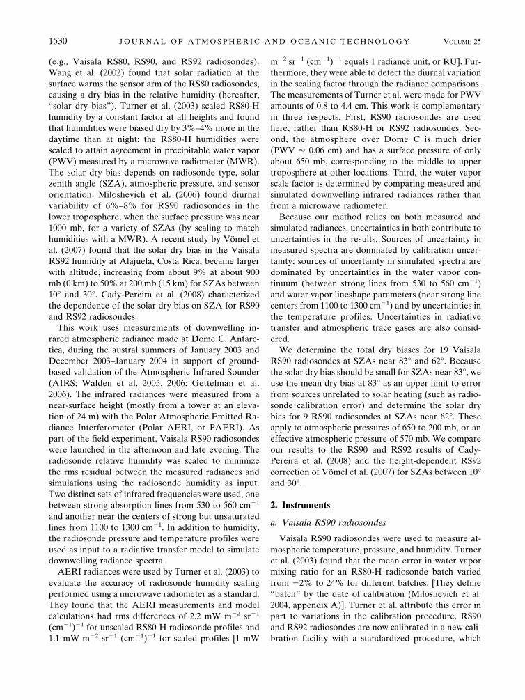
Radiosonde measurements were made during the af-ternoon (around 1600 LT; LT � Local Time � UTC �8), when SZAs were on average 62° (ranging from 59°to 66°), and during the late evening (around 2300 LT),when SZAs were on average 83° (ranging from 81° to85°). Figure 1 shows the profiles of temperature andrelative humidity (RH) with respect to water measuredon 13 January 2004 during the afternoon and late eve-ning. In Fig. 1a, we see that the temperature profiles arealmost identical except near the surface (within the first50 m). By contrast, radiosonde humidities differ mark-

edly (Fig. 1b). The relative humidity at which ice satu-ration occurs for the afternoon temperature profile isalso shown. The ice saturation for the evening tempera-ture profile is almost identical except near the surface,where the ice saturation relative humidity is 72% in-stead of 80%. These radiosoundings are fairly typical ofthose used in this study and will serve as afternoon andevening case studies throughout the rest of this paper.Although the humidity is supersaturated with respect toice at some heights, visual observations and inspectionof concurrent radiances indicate that the sky was clear.Supersaturation with respect to ice is common in theAntarctic atmosphere (Gettelman et al. 2006). Jensenet al. (2001) have reported areas of ice supersaturationnear the tropopause in the absence of ice crystals. Re-gions of supersaturation with respect to ice have alsobeen observed by a water vapor Raman lidar in cloud-free regions in the middle and upper troposphere at amidlatitude site (Comstock et al. 2004).

b. Polar Atmospheric Emitted RadianceInterferometer

The PAERI is an AERI modified for use in polarregions. AERI instruments, developed by the SpaceScience and Engineering Center at the University ofWisconsin in Madison, are ground-based Fourier trans-form infrared spectrometers that remotely sense emis-sion from the atmosphere. The PAERI measureddownwelling infrared radiance in the spectral regionbetween 500 and 3000 cm�1 (3–20 �m) at 1 cm�1 reso-lution for a zenith view. AERI instruments are de-scribed in detail by Knuteson et al. (2004a,b), who in-clude a careful assessment of instrument accuracy thatwe use for estimating our sources of uncertainty. Eachspectrum was generated by taking the Fourier trans-form of an interferogram (Beer 1992) measured by thePAERI; each interferogram is comprised of between 20and 90 consecutive measurements (called coadditions)taken by the interferometer to reduce instrument noise.Spectra of hot and ambient temperature blackbodies ofknown temperature and emissivity are used to calibratemeasurements of the sky, as described by Revercombet al. (1988) and Knuteson et al. (2004b). PAERI mea-surements that were made concurrently with radio-soundings under clear skies were selected for this study.Between 4 and 13 spectra were averaged during theradiosonde flight to further reduce instrument noise.

Figure 2 shows a typical PAERI spectrum. The re-gion of low radiance between 800 and 1300 cm�1 (ex-cluding ozone at 1050 cm�1) is termed the “atmo-spheric window.” Because the Dome C atmosphere isso cold and dry, radiances in the atmospheric windoware very close to zero. The center of the weak CO2 band

FIG. 1. Profiles of (a) temperature and (b) relative humiditywith respect to water (RH) measured by Vaisala RS90 radiosondesat Dome C, Antarctica, on 13 Jan 2004 during the afternoon (1525LT) and evening (2336 LT). The RH at which ice saturation oc-curs for the afternoon temperature profile is also shown.


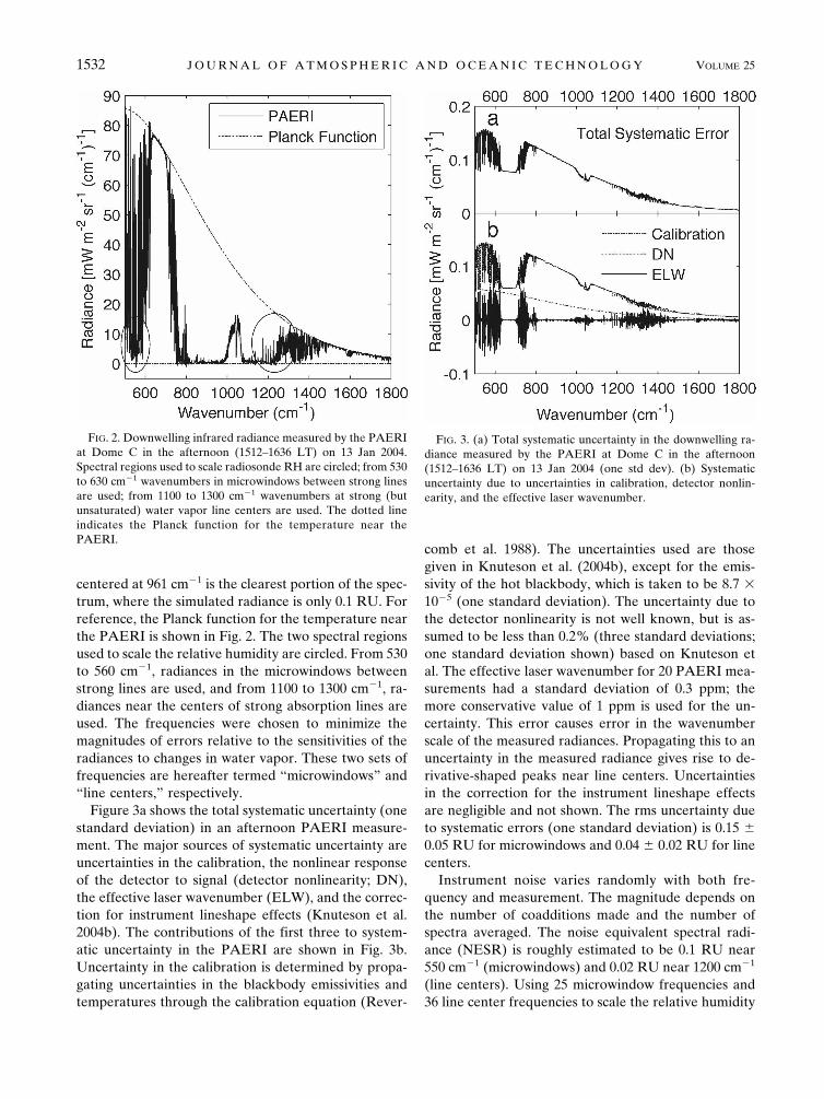
centered at 961 cm�1 is the clearest portion of the spec-trum, where the simulated radiance is only 0.1 RU. Forreference, the Planck function for the temperature nearthe PAERI is shown in Fig. 2. The two spectral regionsused to scale the relative humidity are circled. From 530to 560 cm�1, radiances in the microwindows betweenstrong lines are used, and from 1100 to 1300 cm�1, ra-diances near the centers of strong absorption lines areused. The frequencies were chosen to minimize themagnitudes of errors relative to the sensitivities of theradiances to changes in water vapor. These two sets offrequencies are hereafter termed “microwindows” and“line centers,” respectively.

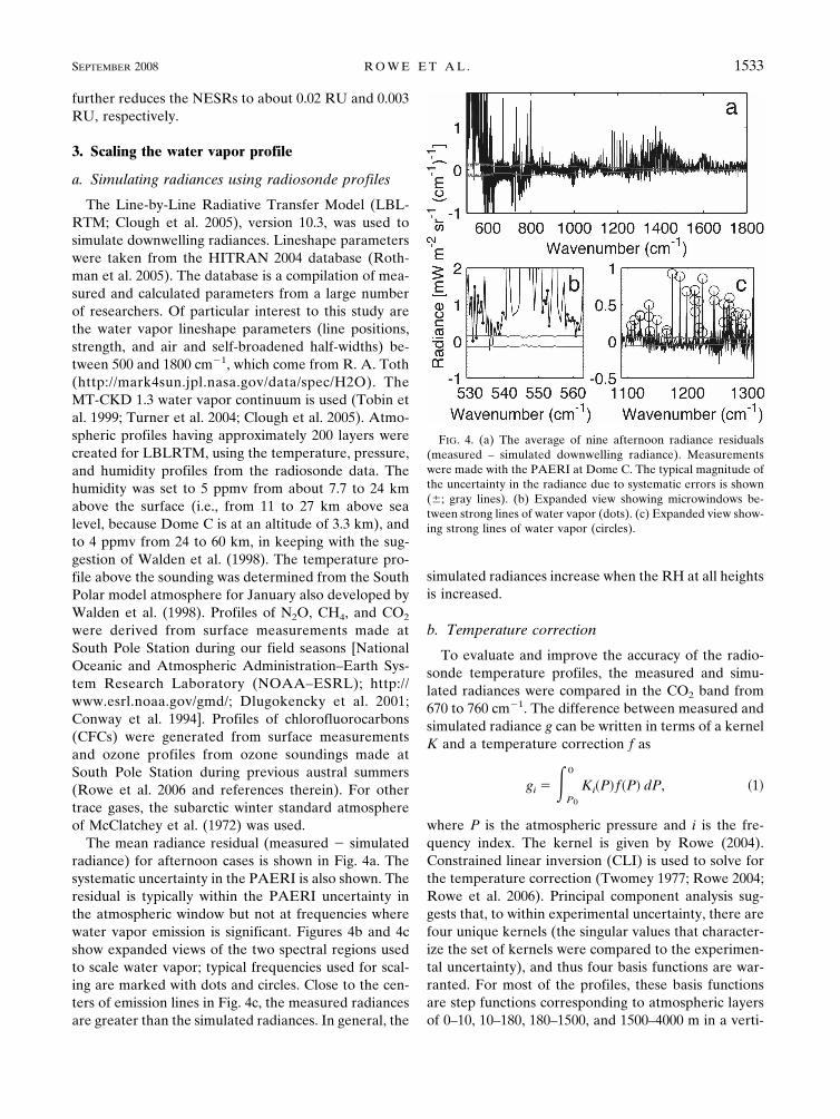
Figure 3a shows the total systematic uncertainty (onestandard deviation) in an afternoon PAERI measure-ment. The major sources of systematic uncertainty areuncertainties in the calibration, the nonlinear responseof the detector to signal (detector nonlinearity; DN),the effective laser wavenumber (ELW), and the correc-tion for instrument lineshape effects (Knuteson et al.2004b). The contributions of the first three to system-atic uncertainty in the PAERI are shown in Fig. 3b.Uncertainty in the calibration is determined by propa-gating uncertainties in the blackbody emissivities andtemperatures through the calibration equation (Rever-

comb et al. 1988). The uncertainties used are thosegiven in Knuteson et al. (2004b), except for the emis-sivity of the hot blackbody, which is taken to be 8.7 �10�5 (one standard deviation). The uncertainty due tothe detector nonlinearity is not well known, but is as-sumed to be less than 0.2% (three standard deviations;one standard deviation shown) based on Knuteson etal. The effective laser wavenumber for 20 PAERI mea-surements had a standard deviation of 0.3 ppm; themore conservative value of 1 ppm is used for the un-certainty. This error causes error in the wavenumberscale of the measured radiances. Propagating this to anuncertainty in the measured radiance gives rise to de-rivative-shaped peaks near line centers. Uncertaintiesin the correction for the instrument lineshape effectsare negligible and not shown. The rms uncertainty dueto systematic errors (one standard deviation) is 0.15 �0.05 RU for microwindows and 0.04 � 0.02 RU for linecenters.

Instrument noise varies randomly with both fre-quency and measurement. The magnitude depends onthe number of coadditions made and the number ofspectra averaged. The noise equivalent spectral radi-ance (NESR) is roughly estimated to be 0.1 RU near550 cm�1 (microwindows) and 0.02 RU near 1200 cm�1

(line centers). Using 25 microwindow frequencies and36 line center frequencies to scale the relative humidity

FIG. 2. Downwelling infrared radiance measured by the PAERIat Dome C in the afternoon (1512–1636 LT) on 13 Jan 2004.Spectral regions used to scale radiosonde RH are circled; from 530to 630 cm�1 wavenumbers in microwindows between strong linesare used; from 1100 to 1300 cm�1 wavenumbers at strong (butunsaturated) water vapor line centers are used. The dotted lineindicates the Planck function for the temperature near thePAERI.

FIG. 3. (a) Total systematic uncertainty in the downwelling ra-diance measured by the PAERI at Dome C in the afternoon(1512–1636 LT) on 13 Jan 2004 (one std dev). (b) Systematicuncertainty due to uncertainties in calibration, detector nonlin-earity, and the effective laser wavenumber.


further reduces the NESRs to about 0.02 RU and 0.003RU, respectively.

3. Scaling the water vapor profile

a. Simulating radiances using radiosonde profiles

The Line-by-Line Radiative Transfer Model (LBL-RTM; Clough et al. 2005), version 10.3, was used tosimulate downwelling radiances. Lineshape parameterswere taken from the HITRAN 2004 database (Roth-man et al. 2005). The database is a compilation of mea-sured and calculated parameters from a large numberof researchers. Of particular interest to this study arethe water vapor lineshape parameters (line positions,strength, and air and self-broadened half-widths) be-tween 500 and 1800 cm�1, which come from R. A. Toth(http://mark4sun.jpl.nasa.gov/data/spec/H2O). TheMT-CKD 1.3 water vapor continuum is used (Tobin etal. 1999; Turner et al. 2004; Clough et al. 2005). Atmo-spheric profiles having approximately 200 layers werecreated for LBLRTM, using the temperature, pressure,and humidity profiles from the radiosonde data. Thehumidity was set to 5 ppmv from about 7.7 to 24 kmabove the surface (i.e., from 11 to 27 km above sealevel, because Dome C is at an altitude of 3.3 km), andto 4 ppmv from 24 to 60 km, in keeping with the sug-gestion of Walden et al. (1998). The temperature pro-file above the sounding was determined from the SouthPolar model atmosphere for January also developed byWalden et al. (1998). Profiles of N2O, CH4, and CO2

were derived from surface measurements made atSouth Pole Station during our field seasons [NationalOceanic and Atmospheric Administration–Earth Sys-tem Research Laboratory (NOAA–ESRL); http://www.esrl.noaa.gov/gmd/; Dlugokencky et al. 2001;Conway et al. 1994]. Profiles of chlorofluorocarbons(CFCs) were generated from surface measurementsand ozone profiles from ozone soundings made atSouth Pole Station during previous austral summers(Rowe et al. 2006 and references therein). For othertrace gases, the subarctic winter standard atmosphereof McClatchey et al. (1972) was used.

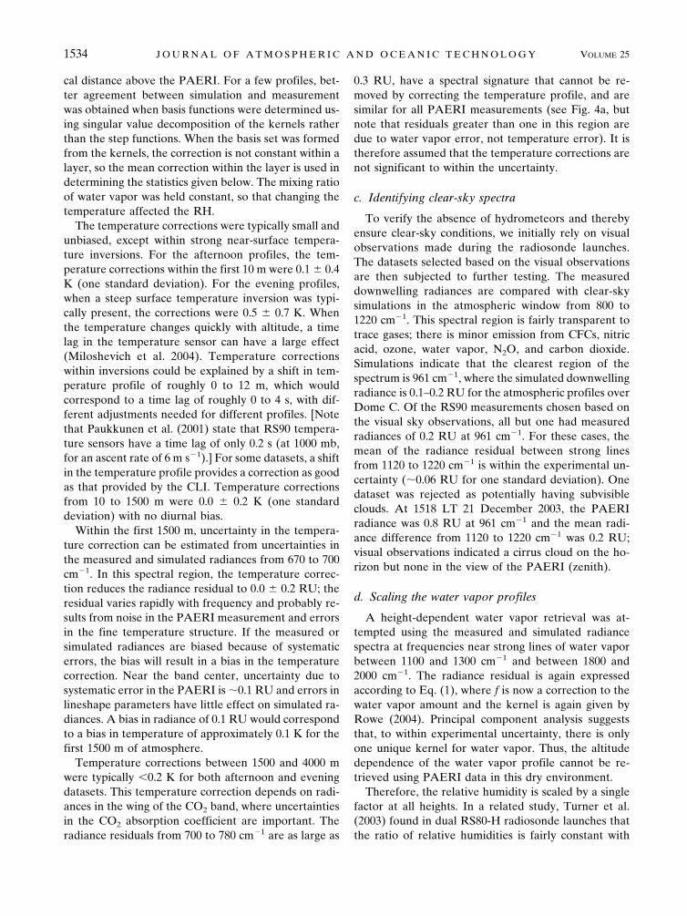
The mean radiance residual (measured � simulatedradiance) for afternoon cases is shown in Fig. 4a. Thesystematic uncertainty in the PAERI is also shown. Theresidual is typically within the PAERI uncertainty inthe atmospheric window but not at frequencies wherewater vapor emission is significant. Figures 4b and 4cshow expanded views of the two spectral regions usedto scale water vapor; typical frequencies used for scal-ing are marked with dots and circles. Close to the cen-ters of emission lines in Fig. 4c, the measured radiancesare greater than the simulated radiances. In general, the

simulated radiances increase when the RH at all heightsis increased.

b. Temperature correction

To evaluate and improve the accuracy of the radio-sonde temperature profiles, the measured and simu-lated radiances were compared in the CO2 band from670 to 760 cm�1. The difference between measured andsimulated radiance g can be written in terms of a kernelK and a temperature correction f as

gi � �P0

0

KiPfP dP, 1

where P is the atmospheric pressure and i is the fre-quency index. The kernel is given by Rowe (2004).Constrained linear inversion (CLI) is used to solve forthe temperature correction (Twomey 1977; Rowe 2004;Rowe et al. 2006). Principal component analysis sug-gests that, to within experimental uncertainty, there arefour unique kernels (the singular values that character-ize the set of kernels were compared to the experimen-tal uncertainty), and thus four basis functions are war-ranted. For most of the profiles, these basis functionsare step functions corresponding to atmospheric layersof 0–10, 10–180, 180–1500, and 1500–4000 m in a verti-

FIG. 4. (a) The average of nine afternoon radiance residuals(measured – simulated downwelling radiance). Measurementswere made with the PAERI at Dome C. The typical magnitude ofthe uncertainty in the radiance due to systematic errors is shown(�; gray lines). (b) Expanded view showing microwindows be-tween strong lines of water vapor (dots). (c) Expanded view show-ing strong lines of water vapor (circles).


cal distance above the PAERI. For a few profiles, bet-ter agreement between simulation and measurementwas obtained when basis functions were determined us-ing singular value decomposition of the kernels ratherthan the step functions. When the basis set was formedfrom the kernels, the correction is not constant within alayer, so the mean correction within the layer is used indetermining the statistics given below. The mixing ratioof water vapor was held constant, so that changing thetemperature affected the RH.

The temperature corrections were typically small andunbiased, except within strong near-surface tempera-ture inversions. For the afternoon profiles, the tem-perature corrections within the first 10 m were 0.1 � 0.4K (one standard deviation). For the evening profiles,when a steep surface temperature inversion was typi-cally present, the corrections were 0.5 � 0.7 K. Whenthe temperature changes quickly with altitude, a timelag in the temperature sensor can have a large effect(Miloshevich et al. 2004). Temperature correctionswithin inversions could be explained by a shift in tem-perature profile of roughly 0 to 12 m, which wouldcorrespond to a time lag of roughly 0 to 4 s, with dif-ferent adjustments needed for different profiles. [Notethat Paukkunen et al. (2001) state that RS90 tempera-ture sensors have a time lag of only 0.2 s (at 1000 mb,for an ascent rate of 6 m s�1).] For some datasets, a shiftin the temperature profile provides a correction as goodas that provided by the CLI. Temperature correctionsfrom 10 to 1500 m were 0.0 � 0.2 K (one standarddeviation) with no diurnal bias.

Within the first 1500 m, uncertainty in the tempera-ture correction can be estimated from uncertainties inthe measured and simulated radiances from 670 to 700cm�1. In this spectral region, the temperature correc-tion reduces the radiance residual to 0.0 � 0.2 RU; theresidual varies rapidly with frequency and probably re-sults from noise in the PAERI measurement and errorsin the fine temperature structure. If the measured orsimulated radiances are biased because of systematicerrors, the bias will result in a bias in the temperaturecorrection. Near the band center, uncertainty due tosystematic error in the PAERI is �0.1 RU and errors inlineshape parameters have little effect on simulated ra-diances. A bias in radiance of 0.1 RU would correspondto a bias in temperature of approximately 0.1 K for thefirst 1500 m of atmosphere.

Temperature corrections between 1500 and 4000 mwere typically �0.2 K for both afternoon and eveningdatasets. This temperature correction depends on radi-ances in the wing of the CO2 band, where uncertaintiesin the CO2 absorption coefficient are important. Theradiance residuals from 700 to 780 cm�1 are as large as

0.3 RU, have a spectral signature that cannot be re-moved by correcting the temperature profile, and aresimilar for all PAERI measurements (see Fig. 4a, butnote that residuals greater than one in this region aredue to water vapor error, not temperature error). It istherefore assumed that the temperature corrections arenot significant to within the uncertainty.

c. Identifying clear-sky spectra

To verify the absence of hydrometeors and therebyensure clear-sky conditions, we initially rely on visualobservations made during the radiosonde launches.The datasets selected based on the visual observationsare then subjected to further testing. The measureddownwelling radiances are compared with clear-skysimulations in the atmospheric window from 800 to1220 cm�1. This spectral region is fairly transparent totrace gases; there is minor emission from CFCs, nitricacid, ozone, water vapor, N2O, and carbon dioxide.Simulations indicate that the clearest region of thespectrum is 961 cm�1, where the simulated downwellingradiance is 0.1–0.2 RU for the atmospheric profiles overDome C. Of the RS90 measurements chosen based onthe visual sky observations, all but one had measuredradiances of 0.2 RU at 961 cm�1. For these cases, themean of the radiance residual between strong linesfrom 1120 to 1220 cm�1 is within the experimental un-certainty (�0.06 RU for one standard deviation). Onedataset was rejected as potentially having subvisibleclouds. At 1518 LT 21 December 2003, the PAERIradiance was 0.8 RU at 961 cm�1 and the mean radi-ance difference from 1120 to 1220 cm�1 was 0.2 RU;visual observations indicated a cirrus cloud on the ho-rizon but none in the view of the PAERI (zenith).

d. Scaling the water vapor profiles

A height-dependent water vapor retrieval was at-tempted using the measured and simulated radiancespectra at frequencies near strong lines of water vaporbetween 1100 and 1300 cm�1 and between 1800 and2000 cm�1. The radiance residual is again expressedaccording to Eq. (1), where f is now a correction to thewater vapor amount and the kernel is again given byRowe (2004). Principal component analysis suggeststhat, to within experimental uncertainty, there is onlyone unique kernel for water vapor. Thus, the altitudedependence of the water vapor profile cannot be re-trieved using PAERI data in this dry environment.

Therefore, the relative humidity is scaled by a singlefactor at all heights. In a related study, Turner et al.(2003) found in dual RS80-H radiosonde launches thatthe ratio of relative humidities is fairly constant with


height, and they scaled the mixing ratio of water vaporto bring the PWV from the radiosonde into agreementwith the PWV from a microwave radiometer. In thisstudy, the radiosonde RH, used to simulate the down-welling radiance, is scaled until the rms difference be-tween the measured and simulated downwelling radi-ance is minimized. The rms difference is

Ey ��1N

i�Mi � Siy�2, 2

where y is the scale factor, M is the measured radiance,S is the simulated radiance, i is the index to frequency,and N is the number of frequencies. Letting “min” rep-resent the minimization operation and defining “inv”such that inv[E(y)] � y(E), we write

y* � inv�min��1N

i�Mi � Siy�2�� . 3

The rms difference is calculated for about 25 frequen-cies in the microwindows between strong lines from 530to 560 cm�1 and for about 40 frequencies near strongline centers of water vapor between 1100 and 1300cm�1. [The frequencies used on 1524 LT (0724 UT) 13January 2004 are listed in Table 1; similar frequenciesare used for all other cases.] The two spectral regionsare complementary in that the water vapor continuumis negligible at the line centers used for the atmosphericconditions experienced at Dome C (Rowe et al. 2006),

but uncertainties in water vapor lineshape parametersare very important; the reverse is true in the micro-windows. The rms differences for all datasets are plot-ted as a function of the relative change in RH (%) inFig. 5. The retrieved water vapor scale factors y* areindicated with stars. Values of y* retrieved using mi-crowindows correspond to rms radiance differences of0.3 to 0.9 RU, and values retrieved using line centerscorrespond to rms radiance differences of 0.1 to 0.2 RU.

Figure 6a shows the mean radiance residual for allafternoon cases after scaling the RH. Figures 6b and 6care expanded views of the two spectral regions used fordetermining the scale factor. Scaling the water vapordecreases the rms difference from 0.8 to 0.5 RU in mi-crowindows and from 0.4 to 0.1 RU at line centers. Theresidual above 1300 cm�1 could be caused by uncer-tainties in the foreign-broadened water vapor con-tinuum. For evening cases the decrease was less dra-matic but resulted in similar reductions in rms differ-ences.

4. Analysis of systematic errors

Calculation of the water vapor scale factor dependson the comparison of measured spectral radiances toradiances simulated using the radiosonde profiles, asshown in Eq. (3). Thus, it is important to accurately

TABLE 1. Frequencies used to scale the water vapor profile for1524 LT 13 Jan 2004. Frequencies used for other datasets aresimilar.

Frequency (cm�1) Frequency (cm�1) Frequency (cm�1)

530.4 530.9 531.3531.8 532.3 532.8533.3 533.8 538.1538.6 539.1 539.5551.1 551.6 552.1552.6 553.0 558.3558.8 559.3 559.8560.3 560.8 561.2561.7 1106.6 1111.4

1121.0 1135.5 1136.01137.4 1149.5 1165.41174.1 1174.5 1186.61187.1 1198.2 1211.21212.1 1212.6 1218.41218.9 1224.7 1225.21244.0 1244.5 1259.91260.4 1268.1 1268.61269.5 1270.0 1271.91280.1 1284.5 1287.41288.3 1290.3 1290.71296.5

FIG. 5. The rms differences between measured and simulateddownwelling radiances as a function of percentage change in rela-tive humidity for clear-sky measurements made at Dome C. OneRU equals 1 mW m�2 sr�1 (cm�1)�1. The water vapor correctionsthat minimize the rms differences are marked with asterisks.


characterize systematic errors in both the PAERI mea-surements and the LBLRTM simulations. Uncertain-ties in the PAERI measurements have been discussedabove and so are only mentioned briefly in this section.Uncertainties in LBLRTM simulations include those

resulting from spectroscopic errors, uncertainties in at-mospheric variables, and radiative transfer errors. Eq.(3) can be rewritten to show the dependence of themeasurement and simulation on parameters relating tothese sources of error; thus,

y* � inv�min��1N

i�Mi � SipWLS, pC, pT, p�CH4�, p�N2O�, pRT, y�2�� ,

where the parameters p that the simulation depends onare, respectively, water vapor lineshape parameters(pWLS), the water vapor continuum (pC), temperature(pT), the atmospheric concentrations of CH4 and N2O(p[CH4] and p[N2O]), and the widths of layers used inperforming the radiative transfer (pRT). Because y* is afunction of many variables, we refer to the most appro-priate value of y* for a given dataset as y�, to avoidconfusion.

The equation for propagation of errors is therefore

�y�2 � ��y*�M�2

�M2 � � �y*

�pWLS�2

�WLS2

� ��y*�pC

�2

�C2 � · · · . 4

We calculate the contribution of the systematic un-certainty in the PAERI measurement by making theapproximation

��y*�M�2

�M2 � y*M � �M � y*M

�M 2

�M2 ,

where, for instance, y*(M) indicates that y* is a func-tion of M. The quantity �M is the total systematic errorin the PAERI spectrum. For convenience, �M is cho-sen to be equal to �M. To get y*(M � �M), the mea-surement is perturbed by �M and the scale factor y* isrecalculated.

The contribution of a source of error in the simulatedradiance to uncertainty in the water vapor scale factoris calculated similarly; thus,

��y*�px

�2

�x2 � �y*�Spx � �x� � y*�Spx��2, 5

where px is a parameter the simulated radiance dependson, such as temperature, and �x is the uncertainty in theparameter.

Tables 2 and 3 summarize uncertainties for micro-windows and line centers. The first column in each tablelists the sources of error. If the source of error is aninput parameter to LBLRTM, the second column liststhe uncertainty in the parameter. The third column liststhe resulting uncertainties in measured or simulated ra-diances in RU; because the uncertainties are frequency-dependent, the rms value for each set of frequencies isgiven. The final column lists the uncertainties in thewater vapor scale factor in units of relative change inRH (%). The standard deviation of the uncertainties inthe scale factor is also given where possible. The lastrow of each table gives the combined uncertainty, cal-culated as the sum of squared uncertainties. Uncertain-ties in the simulated radiance are discussed below.

The temperature correction reduces uncertainties inthe temperature profile to 0.13 K below 1.5 km. Above1.5 km we use the uncertainty (1�) given by Paukkunenet al. (2001) for the Vaisala RS90 radiosonde tempera-tures, 0.25 K.

Emission from the trace gases CH4 and N2O onlyaffects the 1100 to 1300 cm�1 region. Uncertainties inthese trace gases (5%) result in uncertainties in thescale factor of 0.2%.

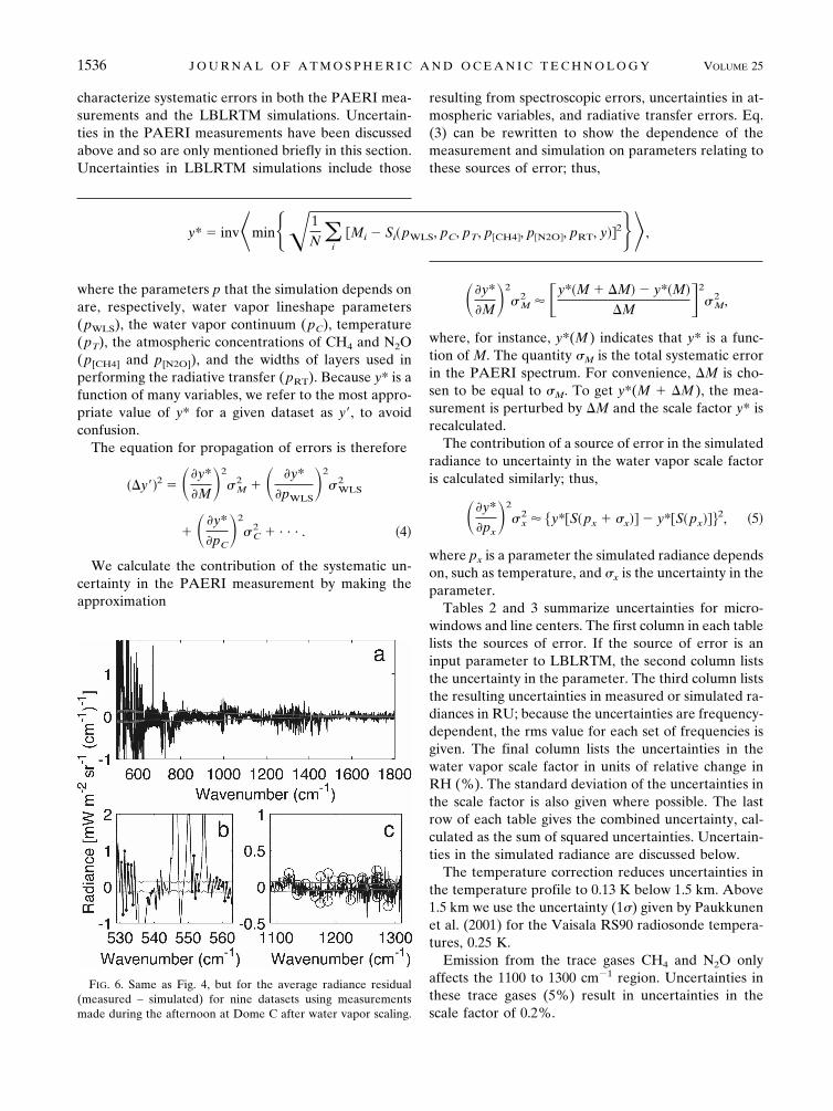
FIG. 6. Same as Fig. 4, but for the average radiance residual(measured – simulated) for nine datasets using measurementsmade during the afternoon at Dome C after water vapor scaling.


Radiative transfer error is mainly due to the finitesize of the atmospheric layers used. Care was taken tominimize this source of error by using nearly 200 layersfor each simulation. The pressure change across eachlayer was 3.5 mb, corresponding to layers of 40 to 100 mthroughout the troposphere. Sensitivity studies wereperformed by comparing simulations at this verticalresolution to simulations at the vertical resolution ofthe radiosonde; as shown in the table, radiative transfererror is a minor contributor to the total error.

Uncertainties in water vapor lineshape parametersneed to be well characterized for results using fre-quencies near line centers. Fortunately, a lot of workhas gone into calculating and measuring water vaporlineshape parameters from 1100 to 1300 cm�1. Uncer-tainty ranges for water vapor line strengths, foreign-broadened line widths, self-broadened line widths, andline positions based on the work of Toth et al. are givenby the HITRAN database (Rothman et al. 2005). Totest the importance of these errors, lineshape param-eters were perturbed by the uncertainties listed, amodified lineshape parameter database was con-structed, and the simulated spectra were recalculated. Itwas determined that uncertainties in air-broadened linewidths (�1%–20%), self-broadened line widths (�1%–10%), and line positions (0.001–0.01 cm�1) are domi-

nated by uncertainties in line strengths (5%–10%). Topropagate errors in line strengths, the uncertainty ineach line strength (�WLS,i) was multiplied by a randomnumber r taken from a normal distribution with a stan-dard deviation of one. Using r�WLS as the uncertaintyin line strength, Eq. (5) was used to solve for the re-sulting uncertainty in the water vapor scale factor forseveral sets of random numbers; the mean values foreach spectral region are reported in Tables 2 and 3.

Uncertainties in the foreign-broadened water vaporcontinuum are important for microwindows. The un-certainty in the foreign-broadened water vapor con-tinuum (MT-CKD 1.3) is estimated to be 20% (Tobinet al. 1999; Clough et al. 2005).

The total uncertainties in the water vapor scale fac-tor, resulting from sources of error that produce bias,are 9% and 4% (relative error in relative humidity) formicrowindows and line centers, respectively.

5. Effective atmospheric pressure

Emission at the frequencies used to scale the relativehumidity is influenced by water vapor throughout thetroposphere. The sensitivity of the downwelling radi-ance to changes in water vapor in atmospheric layerswas investigated to determine the effective height or

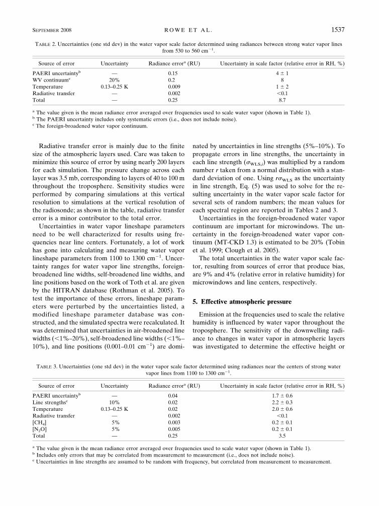
TABLE 2. Uncertainties (one std dev) in the water vapor scale factor determined using radiances between strong water vapor linesfrom 530 to 560 cm�1.

Source of error Uncertainty Radiance errora (RU) Uncertainty in scale factor (relative error in RH, %)

PAERI uncertaintyb — 0.15 4 � 1WV continuumc 20% 0.2 8Temperature 0.13–0.25 K 0.009 1 � 2Radiative transfer — 0.002 �0.1Total — 0.25 8.7

a The value given is the mean radiance error averaged over frequencies used to scale water vapor (shown in Table 1).b The PAERI uncertainty includes only systematic errors (i.e., does not include noise).c The foreign-broadened water vapor continuum.

TABLE 3. Uncertainties (one std dev) in the water vapor scale factor determined using radiances near the centers of strong watervapor lines from 1100 to 1300 cm�1.

Source of error Uncertainty Radiance errora (RU) Uncertainty in scale factor (relative error in RH, %)

PAERI uncertaintyb — 0.04 1.7 � 0.6Line strengthsc 10% 0.02 2.2 � 0.3Temperature 0.13–0.25 K 0.02 2.0 � 0.6Radiative transfer — 0.002 �0.1[CH4] 5% 0.003 0.2 � 0.1[N2O] 5% 0.005 0.2 � 0.1Total — 0.25 3.5

a The value given is the mean radiance error averaged over frequencies used to scale water vapor (shown in Table 1).b Includes only errors that may be correlated from measurement to measurement (i.e., does not include noise).c Uncertainties in line strengths are assumed to be random with frequency, but correlated from measurement to measurement.


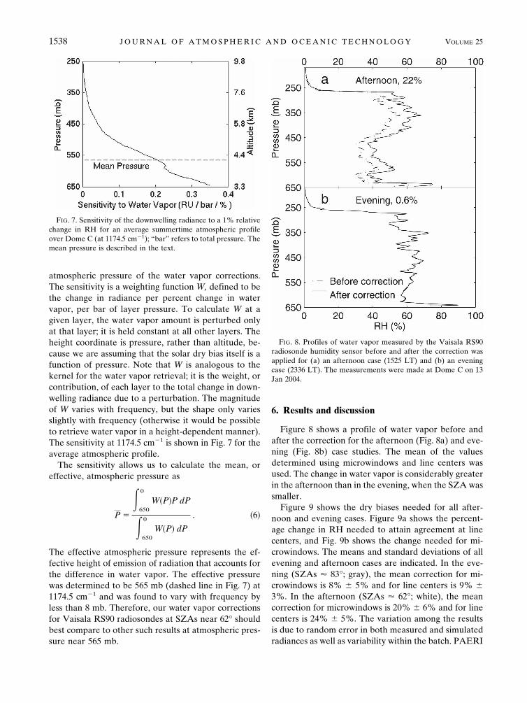
atmospheric pressure of the water vapor corrections.The sensitivity is a weighting function W, defined to bethe change in radiance per percent change in watervapor, per bar of layer pressure. To calculate W at agiven layer, the water vapor amount is perturbed onlyat that layer; it is held constant at all other layers. Theheight coordinate is pressure, rather than altitude, be-cause we are assuming that the solar dry bias itself is afunction of pressure. Note that W is analogous to thekernel for the water vapor retrieval; it is the weight, orcontribution, of each layer to the total change in down-welling radiance due to a perturbation. The magnitudeof W varies with frequency, but the shape only variesslightly with frequency (otherwise it would be possibleto retrieve water vapor in a height-dependent manner).The sensitivity at 1174.5 cm�1 is shown in Fig. 7 for theaverage atmospheric profile.

The sensitivity allows us to calculate the mean, oreffective, atmospheric pressure as

P �

�650

0

WPP dP

�650

0

WP dP

. 6

The effective atmospheric pressure represents the ef-fective height of emission of radiation that accounts forthe difference in water vapor. The effective pressurewas determined to be 565 mb (dashed line in Fig. 7) at1174.5 cm�1 and was found to vary with frequency byless than 8 mb. Therefore, our water vapor correctionsfor Vaisala RS90 radiosondes at SZAs near 62° shouldbest compare to other such results at atmospheric pres-sure near 565 mb.

6. Results and discussion

Figure 8 shows a profile of water vapor before andafter the correction for the afternoon (Fig. 8a) and eve-ning (Fig. 8b) case studies. The mean of the valuesdetermined using microwindows and line centers wasused. The change in water vapor is considerably greaterin the afternoon than in the evening, when the SZA wassmaller.

Figure 9 shows the dry biases needed for all after-noon and evening cases. Figure 9a shows the percent-age change in RH needed to attain agreement at linecenters, and Fig. 9b shows the change needed for mi-crowindows. The means and standard deviations of allevening and afternoon cases are indicated. In the eve-ning (SZAs � 83°; gray), the mean correction for mi-crowindows is 8% � 5% and for line centers is 9% �3%. In the afternoon (SZAs � 62°; white), the meancorrection for microwindows is 20% � 6% and for linecenters is 24% � 5%. The variation among the resultsis due to random error in both measured and simulatedradiances as well as variability within the batch. PAERI

FIG. 7. Sensitivity of the downwelling radiance to a 1% relativechange in RH for an average summertime atmospheric profileover Dome C (at 1174.5 cm�1); “bar” refers to total pressure. Themean pressure is described in the text.

FIG. 8. Profiles of water vapor measured by the Vaisala RS90radiosonde humidity sensor before and after the correction wasapplied for (a) an afternoon case (1525 LT) and (b) an eveningcase (2336 LT). The measurements were made at Dome C on 13Jan 2004.


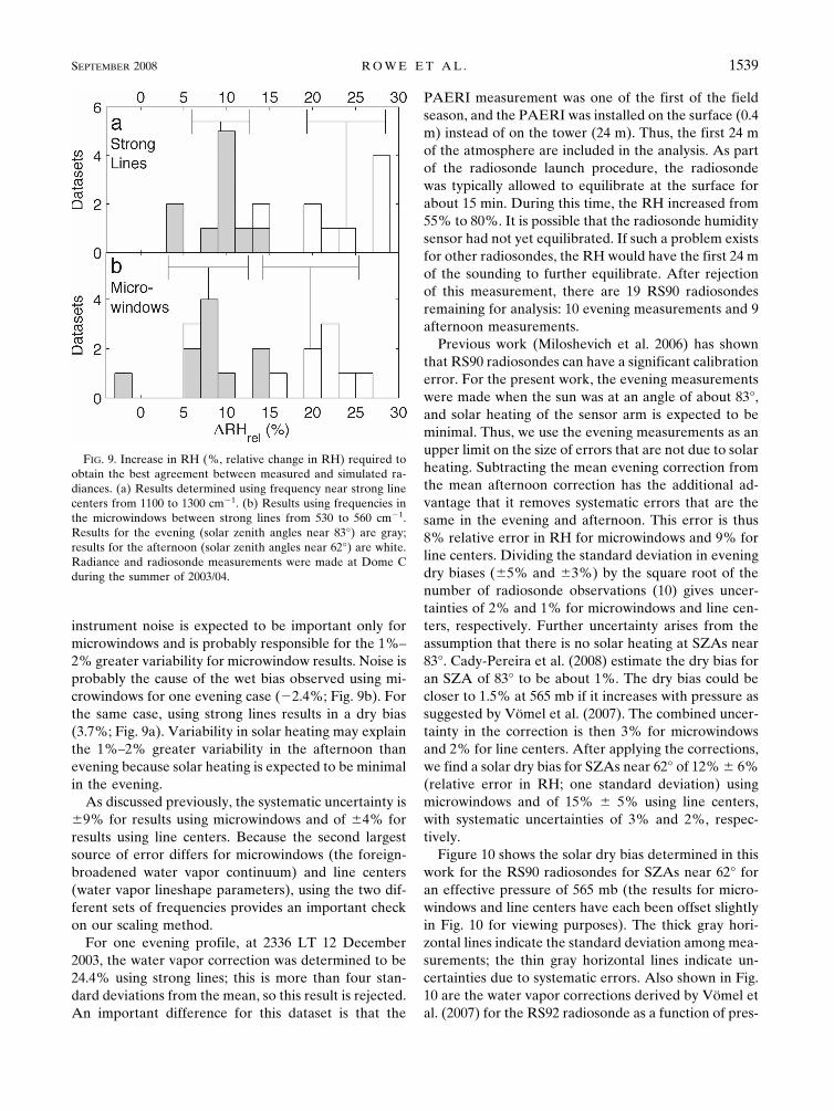
instrument noise is expected to be important only formicrowindows and is probably responsible for the 1%–2% greater variability for microwindow results. Noise isprobably the cause of the wet bias observed using mi-crowindows for one evening case (�2.4%; Fig. 9b). Forthe same case, using strong lines results in a dry bias(3.7%; Fig. 9a). Variability in solar heating may explainthe 1%–2% greater variability in the afternoon thanevening because solar heating is expected to be minimalin the evening.

As discussed previously, the systematic uncertainty is�9% for results using microwindows and of �4% forresults using line centers. Because the second largestsource of error differs for microwindows (the foreign-broadened water vapor continuum) and line centers(water vapor lineshape parameters), using the two dif-ferent sets of frequencies provides an important checkon our scaling method.

For one evening profile, at 2336 LT 12 December2003, the water vapor correction was determined to be24.4% using strong lines; this is more than four stan-dard deviations from the mean, so this result is rejected.An important difference for this dataset is that the

PAERI measurement was one of the first of the fieldseason, and the PAERI was installed on the surface (0.4m) instead of on the tower (24 m). Thus, the first 24 mof the atmosphere are included in the analysis. As partof the radiosonde launch procedure, the radiosondewas typically allowed to equilibrate at the surface forabout 15 min. During this time, the RH increased from55% to 80%. It is possible that the radiosonde humiditysensor had not yet equilibrated. If such a problem existsfor other radiosondes, the RH would have the first 24 mof the sounding to further equilibrate. After rejectionof this measurement, there are 19 RS90 radiosondesremaining for analysis: 10 evening measurements and 9afternoon measurements.

Previous work (Miloshevich et al. 2006) has shownthat RS90 radiosondes can have a significant calibrationerror. For the present work, the evening measurementswere made when the sun was at an angle of about 83°,and solar heating of the sensor arm is expected to beminimal. Thus, we use the evening measurements as anupper limit on the size of errors that are not due to solarheating. Subtracting the mean evening correction fromthe mean afternoon correction has the additional ad-vantage that it removes systematic errors that are thesame in the evening and afternoon. This error is thus8% relative error in RH for microwindows and 9% forline centers. Dividing the standard deviation in eveningdry biases (�5% and �3%) by the square root of thenumber of radiosonde observations (10) gives uncer-tainties of 2% and 1% for microwindows and line cen-ters, respectively. Further uncertainty arises from theassumption that there is no solar heating at SZAs near83°. Cady-Pereira et al. (2008) estimate the dry bias foran SZA of 83° to be about 1%. The dry bias could becloser to 1.5% at 565 mb if it increases with pressure assuggested by Vömel et al. (2007). The combined uncer-tainty in the correction is then 3% for microwindowsand 2% for line centers. After applying the corrections,we find a solar dry bias for SZAs near 62° of 12% � 6%(relative error in RH; one standard deviation) usingmicrowindows and of 15% � 5% using line centers,with systematic uncertainties of 3% and 2%, respec-tively.

Figure 10 shows the solar dry bias determined in thiswork for the RS90 radiosondes for SZAs near 62° foran effective pressure of 565 mb (the results for micro-windows and line centers have each been offset slightlyin Fig. 10 for viewing purposes). The thick gray hori-zontal lines indicate the standard deviation among mea-surements; the thin gray horizontal lines indicate un-certainties due to systematic errors. Also shown in Fig.10 are the water vapor corrections derived by Vömel etal. (2007) for the RS92 radiosonde as a function of pres-

FIG. 9. Increase in RH (%, relative change in RH) required toobtain the best agreement between measured and simulated ra-diances. (a) Results determined using frequency near strong linecenters from 1100 to 1300 cm�1. (b) Results using frequencies inthe microwindows between strong lines from 530 to 560 cm�1.Results for the evening (solar zenith angles near 83°) are gray;results for the afternoon (solar zenith angles near 62°) are white.Radiance and radiosonde measurements were made at Dome Cduring the summer of 2003/04.


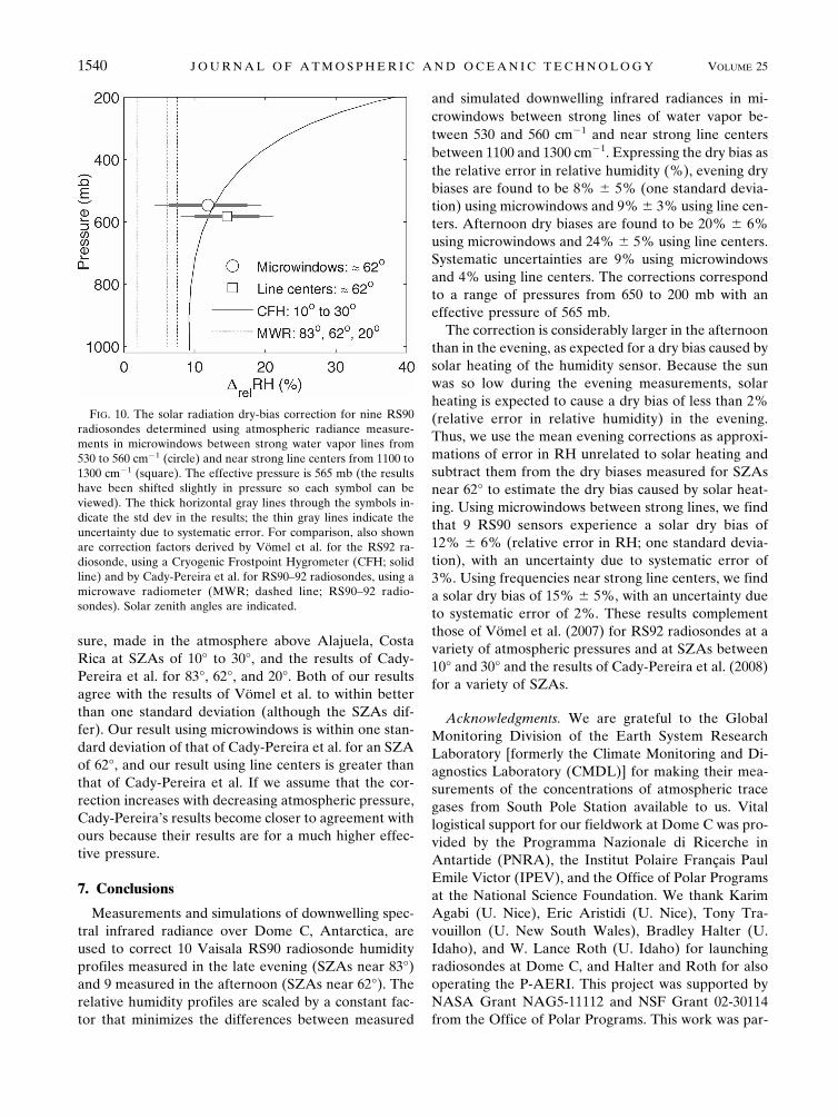
sure, made in the atmosphere above Alajuela, CostaRica at SZAs of 10° to 30°, and the results of Cady-Pereira et al. for 83°, 62°, and 20°. Both of our resultsagree with the results of Vömel et al. to within betterthan one standard deviation (although the SZAs dif-fer). Our result using microwindows is within one stan-dard deviation of that of Cady-Pereira et al. for an SZAof 62°, and our result using line centers is greater thanthat of Cady-Pereira et al. If we assume that the cor-rection increases with decreasing atmospheric pressure,Cady-Pereira’s results become closer to agreement withours because their results are for a much higher effec-tive pressure.

7. Conclusions

Measurements and simulations of downwelling spec-tral infrared radiance over Dome C, Antarctica, areused to correct 10 Vaisala RS90 radiosonde humidityprofiles measured in the late evening (SZAs near 83°)and 9 measured in the afternoon (SZAs near 62°). Therelative humidity profiles are scaled by a constant fac-tor that minimizes the differences between measured

and simulated downwelling infrared radiances in mi-crowindows between strong lines of water vapor be-tween 530 and 560 cm�1 and near strong line centersbetween 1100 and 1300 cm�1. Expressing the dry bias asthe relative error in relative humidity (%), evening drybiases are found to be 8% � 5% (one standard devia-tion) using microwindows and 9% � 3% using line cen-ters. Afternoon dry biases are found to be 20% � 6%using microwindows and 24% � 5% using line centers.Systematic uncertainties are 9% using microwindowsand 4% using line centers. The corrections correspondto a range of pressures from 650 to 200 mb with aneffective pressure of 565 mb.

The correction is considerably larger in the afternoonthan in the evening, as expected for a dry bias caused bysolar heating of the humidity sensor. Because the sunwas so low during the evening measurements, solarheating is expected to cause a dry bias of less than 2%(relative error in relative humidity) in the evening.Thus, we use the mean evening corrections as approxi-mations of error in RH unrelated to solar heating andsubtract them from the dry biases measured for SZAsnear 62° to estimate the dry bias caused by solar heat-ing. Using microwindows between strong lines, we findthat 9 RS90 sensors experience a solar dry bias of12% � 6% (relative error in RH; one standard devia-tion), with an uncertainty due to systematic error of3%. Using frequencies near strong line centers, we finda solar dry bias of 15% � 5%, with an uncertainty dueto systematic error of 2%. These results complementthose of Vömel et al. (2007) for RS92 radiosondes at avariety of atmospheric pressures and at SZAs between10° and 30° and the results of Cady-Pereira et al. (2008)for a variety of SZAs.

Acknowledgments. We are grateful to the GlobalMonitoring Division of the Earth System ResearchLaboratory [formerly the Climate Monitoring and Di-agnostics Laboratory (CMDL)] for making their mea-surements of the concentrations of atmospheric tracegases from South Pole Station available to us. Vitallogistical support for our fieldwork at Dome C was pro-vided by the Programma Nazionale di Ricerche inAntartide (PNRA), the Institut Polaire Français PaulEmile Victor (IPEV), and the Office of Polar Programsat the National Science Foundation. We thank KarimAgabi (U. Nice), Eric Aristidi (U. Nice), Tony Tra-vouillon (U. New South Wales), Bradley Halter (U.Idaho), and W. Lance Roth (U. Idaho) for launchingradiosondes at Dome C, and Halter and Roth for alsooperating the P-AERI. This project was supported byNASA Grant NAG5-11112 and NSF Grant 02-30114from the Office of Polar Programs. This work was par-

FIG. 10. The solar radiation dry-bias correction for nine RS90radiosondes determined using atmospheric radiance measure-ments in microwindows between strong water vapor lines from530 to 560 cm�1 (circle) and near strong line centers from 1100 to1300 cm�1 (square). The effective pressure is 565 mb (the resultshave been shifted slightly in pressure so each symbol can beviewed). The thick horizontal gray lines through the symbols in-dicate the std dev in the results; the thin gray lines indicate theuncertainty due to systematic error. For comparison, also shownare correction factors derived by Vömel et al. for the RS92 ra-diosonde, using a Cryogenic Frostpoint Hygrometer (CFH; solidline) and by Cady-Pereira et al. for RS90–92 radiosondes, using amicrowave radiometer (MWR; dashed line; RS90–92 radio-sondes). Solar zenith angles are indicated.


tially supported by the U.S. Department of Energy,Office of Science, Office of Biological and Environ-mental Research, Environmental Sciences Division aspart of the Atmospheric Radiation Measurement(ARM) program via Grant DE-FG02-06ER64167.

REFERENCES

Beer, R., 1992: Remote Sensing by Fourier Transform Spectrosco-py. Academic Press, 153 pp.

Cady-Pereira, K. E., M. W. Shephard, D. D. Turner, E. J. Mlawer,S. A. Clough, and T. J. Wagner, 2008: Improved daytime col-umn-integrated precipitable water vapor from Vaisala radio-sonde humidity sensors. J. Atmos. Oceanic Technol., 25, 873–883.

Clough, S. A., M. W. Shephard, E. J. Mlawer, J. S. Delamere,M. J. Iacono, K. Cady-Pereira, S. Boukabara, and P. D.Brown, 2005: Atmospheric radiative transfer modeling: Asummary of the AER codes. J. Quant. Spectrosc. Radiat.Transfer, 91, 233–244.

Comstock, J. M., T. P. Ackerman, and D. D. Turner, 2004: Evi-dence of high ice supersaturation in cirrus clouds using ARMRaman lidar measurements. Geophys. Res. Lett., 31, L11106,doi:10.1029/2004GL019705.

Conway, T. J., P. P. Tans, L. S. Waterman, K. W. Thoning, D. R.Kitzis, K. A. Masarie, and N. Zhang, 1994: Evidence for in-terannual variability of the carbon cycle from the NOAA/CMDL global air sampling network. J. Geophys. Res., 99,22 831–22 855.

Dlugokencky, E. J., B. P. Walter, K. A. Masarie, P. M. Lang, andE. S. Kasischke, 2001: Measurements of an anomalous globalmethane increase during 1998. Geophys. Res. Lett., 28, 499–502.

Ferrare, R. A., and Coauthors, 2004: Characterization of uppertropospheric water vapor measurements during AFWEX us-ing LASE. J. Atmos. Oceanic Technol., 21, 1790–1808.

Gettelman, A., V. P. Walden, L. M. Miloshevich, W. L. Roth, andB. Halter, 2006: Relative humidity over Antarctica from ra-diosondes, satellites, and a general circulation model. J. Geo-phys. Res., 111, D09S13, doi:10.1029/2005JD006636.

Held, I. M., and B. J. Soden, 2000: Water vapor feedback andglobal warming. Annu. Rev. Energy Environ., 25, 441–475.

Hudson, S. R., M. S. Town, V. P. Walden, and S. G. Warren, 2004:Temperature, humidity, and pressure response of radio-sondes at low temperatures. J. Atmos. Oceanic Technol., 21,825–836.

Jensen, E. J., and Coauthors, 2001: Prevalence of ice-super-saturated regions in the upper troposphere: Implications foroptically thin ice cloud formation. J. Geophys. Res., 106,17 253–17 266.

Knuteson, R. O., and Coauthors, 2004a: Atmospheric EmittedRadiance Interferometer. Part I: Instrument design. J. At-mos. Oceanic Technol., 21, 1763–1776.

——, and Coauthors, 2004b: Atmospheric Emitted Radiance In-terferometer. Part II: Instrument performance. J. Atmos.Oceanic Technol., 21, 1777–1789.

McClatchey, R. A., R. W. Fenn, J. E. A. Selby, F. E. Volz, andJ. S. Garing, 1972: Optical properties of the atmosphere. 3rded. Tech. Rep. AFCRL-72-0497, Air Force GeophysicalLaboratories, 108 pp.

Miloshevich, L. M., H. Vömel, A. Paukkunen, A. J. Heymsfield,and S. J. Oltmans, 2001: Characterization and correction ofrelative humidity measurements from Vaisala RS80-A radio-sondes at cold temperatures. J. Atmos. Oceanic Technol., 18,135–156.

——, A. Paukkunen, H. Vömel, and S. J. Oltmans, 2004: Devel-opment and validation of a time-lag correction for Vaisalaradiosonde humidity measurements. J. Atmos. Oceanic Tech-nol., 21, 1305–1327.

——, H. Vömel, D. N. Whiteman, B. M. Lesht, F. J. Schmidlinand F. Russo, 2006: Absolute accuracy of water vapor mea-surements from six operational radiosonde types launchedduring AWEX-G and implications for AIRS validation. J.Geophys. Res., 111, D09S10, doi:10.1029/2005JD006083.

Paukkunen, A., V. Antikainen, and H. Jauhiainen, 2001: Accu-racy and performance of the new Vaisala RS90 radiosonde inoperational use. Preprints, 11th Symp. on Meteorological Ob-servations and Instrumentation, Albuquerque, NM, Amer.Meteor. Soc., 4.5.

Revercomb, H. E., H. Buijs, H. B. Howell, D. D. LaPorte, W. L.Smith, and L. A. Sromovsky, 1988: Radiometric calibrationof IR Fourier transform spectrometers: Solution to a problemwith the High-Resolution Interferometer Sounder. Appl.Opt., 27, 3210–3218.

Rothman, L. S., and Coauthors, 2005: The HITRAN 2004 mo-lecular spectroscopic database. J. Quant. Spectrosc. Radiat.Transfer, 96, 139–204.

Rowe, P. M., 2004: Measurements of the foreign-broadened con-tinuum of water vapor in the 6.3-micron band at �30° Cel-sius. Ph.D. thesis, University of Washington, 278 pp.

——, V. P. Walden, and S. G. Warren, 2006: Measurements of theforeign-broadened continuum of water vapor in the 6.3-�mband at �30°C. Appl. Opt., 45, 4366–4382.

Sinha, A., and J. E. Harries, 1995: Water vapour and greenhousetrapping: The role of far infrared absorption. Geophys. Res.Lett., 22, 2147–2150.

Tobin, D. C., and Coauthors, 1999: Downwelling spectral radi-ance observations at the SHEBA ice station: Water vaporcontinuum measurements from 17 to 26 �m. J. Geophys. Res.,104 (D2), 2081–2092.

Turner, D. D., B. M. Lesht, S. A. Clough, J. C. Liljegren, H. E.Revercomb, and D. C. Tobin, 2003: Dry bias and variabilityin Vaisala RS80-H radiosondes: The ARM experience. J. At-mos. Oceanic Technol., 20, 117–132.

——, and Coauthors, 2004: The QME AERI LBLRTM: A closureexperiment for downwelling high spectral resolution infraredradiance. J. Atmos. Sci., 61, 2657–2675.

Twomey, S., 1977: Introduction to the Mathematics of Inversion inRemote Sensing and Indirect Measurements. Elsevier, 243 pp.

Vömel, H., and Coauthors, 2007: Radiation dry bias of the VaisalaRS92 humidity sensor. J. Atmos. Oceanic Technol., 24, 953–963.

Walden, V. P., S. G. Warren, and F. J. Murcray, 1998: Measure-ments of the downward longwave radiation spectrum overthe Antarctic Plateau and comparisons to a line-by-line ra-diative transfer model for clear skies. J. Geophys. Res., 103,3825–3846.

——, M. S. Town, B. Halter, and J. W. V. Storey, 2005: Firstmeasurements of the infrared sky brightness at Dome C,Antarctica. Publ. Astron. Soc. Pacific, 117, 300–308.

——, W. L. Roth, R. S. Stone, and B. Halter, 2006: Radiometricvalidation of the Atmospheric Infrared Sounder over theAntarctic Plateau. J. Geophys. Res., 111, D09S03,doi:10.1029/2005JD006357.

Wang, J., H. L. Cole, D. J. Carlson, E. R. Miller, K. Beierle, A.Paukkunen, and T. K. Laine, 2002: Corrections of humiditymeasurement errors from the Vaisala RS80 radiosonde: Ap-plication to TOGA COARE data. J. Atmos. Oceanic Tech-nol., 19, 981–1002.


Documents

Dry Bias in Vaisala RS90 Radiosonde Humidity Profiles …vonw/pubs/RoweEtAl_JTech_2008.pdfTwo distinct sets of infrared frequencies were used, one between strong absorption lines from