1

Brier Skill Scores, ROCs, and Economic Value Diagrams

Can Overestimate Forecast Skill

Thomas M. Hamill

NOAA-CIRES Climate Diagnostics Center, Boulder, Colorado

Josip Juras

Geophysical Institute, Faculty of Science, University of Zagreb

Zagreb, Croatia

DRAFT

To be submitted as a NOTE to Monthly Weather Review

13 April 2005

Corresponding author address:

Dr. Thomas M. Hamill NOAA-CIRES Climate Diagnostics Center

R/CDC 1, 325 Broadway Boulder, CO 80301 USA

e-mail: tom.hamill@noaa.gov

phone: 1 (303) 497-3060

2

ABSTRACT

The Brier skill score, relative operating characteristic (ROC), and economic value

diagrams are commonly used by the weather forecast community as tools for

probabilistic forecast verification. Unfortunately, all may provide unduly optimistic

estimates of forecast skill if their computation follows procedures that implicitly assume

that the climatology does not vary among samples. In computing the Brier skill score, if

the Brier score of the reference climatological forecast assumes the climatology event

probability is the same over all forecast samples when it is not, false skill may be

reported. For the ROC and economic value diagrams, false skill can be reported when

the contingency tables underlying these scores are populated with samples with differing

climatologies. An explanation of this false skill is provided, as well as guidelines for

how to adapt these diagnostics to avoid this problem.

3

1. Introduction

For much of the history of numerical weather prediction, the primary motivation has

been to improve deterministic weather forecasts. With the advent of ensemble forecast

techniques, there has been a renewed interest in improving probabilistic weather forecasts

and the methods for verifying these forecasts. Ensemble forecast verification has inherited

several metrics for probabilistic forecast verification, and many new ones have been

developed or adapted in recent years. We continue to learn about what these diagnostics are

telling us about ensemble forecasts.

The question to be addressed in this note is whether several commonly used ensemble

forecast verification metrics correctly report no forecast skill when none exists. This is

motivated by our own experiences of diagnosing unexpected positive skill. Examples can be

found in the open literature as well. For example, Buizza et al. (1999) verified their

ensemble forecasts in many ways. They found that some of their scores did not approach the

expected asymptotic value associated with no skill as forecast lead increased and the

forecasts increasingly resembled random samples from climatology. Juras (2000) offered a

possible explanation in a comment on this article, suggesting that the chosen metrics might

report false skill if climatological frequencies vary within the verification area.

This note extends the comments of Juras (2000). We choose to examine three

common skill metrics, the Brier skill score (Wilks 1995), the relative operating characteristic

(ROC; Swets 1973, Harvey et al. 1992), and economic value diagrams (Richardson 2000).

All may be sensitive to reporting forecast skill when none is present. Other metrics such as

the ranked probability skill score (Epstein 1969, Murphy 1971, Wilks 1995) will not be

discussed but are subject to the same problem.

4

Below, section 2 will provide a brief review of the Brier skill score, the ROC, and

economic value diagrams, as well as the mechanics for how they are generated with

ensemble forecasts. Section 3 follows with a very simple example of false skill and an

explanation of why it occurs. Section 4 shows that the false value may or may not be

reported with real meteorological data, depending on what event is being considered.

Section 5 concludes with a discussion of the implications of this problem.

2. Brier skill score, ROC, and economic value diagrams Brier scores (Brier 1950) and Brier skill scores have been used for decades. The

Brier score is a measure of the mean-square error of probability forecasts for a dichotomous

(two-category) event, such as the occurrence/non-occurrence of precipitation. A review is

provided in Wilks (1995), and references therein provide further background. The Brier

score is often hard to interpret; is a Brier score of 0.6 good or bad? Consequently, the Brier

score is often converted to a skill score, normalizing the score by that of a reference forecast

such as climatology (ibid). A Brier skill score (BSS) of 1.0 indicates a perfect forecast, while

a BSS of 0.0 should indicate the skill of the reference forecast.

The relative operating characteristic (ROC) and economic value diagrams have

gained widespread acceptance in the past few years as tools for ensemble verification. The

ROC has been used for decades in engineering and biomedical and psychology applications;

see an overview in Swets (1973). Its application in meteorology was proposed in Mason

(1982), Stanski et al. (1989), and Harvey et al. (1992). In the Hamill et al. (2000a) summary

of an ensemble workshop, it was recommended as a standard verification metric, and this the

ROC was recently made part of the World Meteorological Organization’s (WMO) standard

5

ensemble verification metrics (WMO, 1992). Characteristics of the ROC have been

discussed in Mason and Graham (1999), Juras (2000), Wilson (2000), Buizza et al. (2000),

Wilks (2001), Kheshgi and White (2001), Kharin and Zwiers (2003), and Marzban (2004).

The technique has been used to diagnose forecast accuracy in, for example, Buizza and

Palmer (1998), Buizza et al. (1999), Hamill et al. (2000b), Palmer et al. (2000), Richardson

(2000, 2001ab), Wandishin et al. (2001), Mullen and Buizza (2001, 2002), Bright and Mullen

(2002), Yang and Arritt (2002), Legg and Mylne (2004), Zhu et al. (2002), and Gallus and

Segal (2004).

Economic value diagrams were introduced to the meteorology community by

Richardson (2000). These diagrams provide information about the potential economic

value of ensemble forecasts for a particular event. The diagrams indicate the relative

value as a function of the user’s cost/loss ratio. A value of 1.0 indicates that the full

economic value of a perfect forecast should be realized, and a value of 0.0 indicates the

value of climatology. This framework was also used in Palmer et al. (2000) and

Richardson (2001). Demonstrations of its application value can be found, for instance, in

Richardson (2000), Palmer et al. (2000), Buizza et al. (2003), and Zhu et al. (2002).

A review of the statistical theory underlying the ROC and economic value

diagrams can be found in other sources. Harvey et al. (1992) provide a thorough review

of the concepts underlying the ROC, and Richardson (2000) and Zhu et al. (2002) explain

economic value diagrams. Here we provide only the mechanics of how to generate these

diagrams from ensemble forecasts.

6

Start by defining a dichotomous event of interest. Let Xe(j,k) = [X1(j,k), … ,

Xn(j,k)] be an n-member ensemble forecast for the jth of m locations and the kth of r case

days, sorted from lowest to highest. This sorted ensemble is then converted into an n-

member binary forecast Ie(j,k) = [I1(j,k), … , In (j,k)] indicating whether the event was

forecast (=1) or not forecast (=0) in each member. The observed weather is also noted

and converted to binary, denoted by Io(j,k).

a. Brier skill scores

Assuming that each member forecast is equally likely, a forecast probability

pf(j,k) is calculated from the dichotomized ensemble:

pf (j,k) = Ii ( j,k)i=1

n

!n

. (1)

The Brier score of the forecast BSf is calculated as

BSf =k=1

r

! pf ( j,k) " Io( j,k)( )2

j=1

m

! . (2)

A Brier skill score (BSS) is calculated as

BSS = 1.0 – BSf / BSr , (3)

where BSr is the Brier score of the reference probability forecast, typically the probability

of event occurrence from climatology.

An ambiguity and potential source of false skill may be traced to the method for

calculating BSr, to be illustrated in sections 3 and 4. One method would be to generate a

climatological probability pc(j) of event occurrence unique to each location of the m

locations in the domain,

7

pc ( j) =

Iok=1

r

! j,k( )

r, (4)

in which case BSr would be

BSr = pc j( ) ! Io j,k( )( )j=1

m

"k=1

r

"2

. (5)

Another way would be to calculate a climatology pc averaged over all locations

pc =

Io j,k( )j=1

m

!k=1

r

!

r "m , (6)

and let

BSr = pc ! Io j,k( )( )j=1

m

"k=1

r

"2

. (7)

b. ROC diagrams

Calculation of the ROC starts with the population of 2x2 contingency tables, with

separate contingency tables tallied for each sorted ensemble member and location. The

contingency table for the jth location and ith sorted ensemble member has four elements:

Γi(j) = [ ai(j), bi(j), ci(j), di(j)], indicating the relative fraction of hits, misses, false alarms,

and correct rejections (Table 1). The contingency table is populated using data over all r

case days, and then each is normalized so the sum of the elements is 1.0.

The hit rate (HR) for the ith sorted forecast and jth location is defined as

HRi (j) = ai (j) / (ai(j) +ci(j)). (8)

Similarly, the false alarm rate for the ith sorted forecast is defined as

FARi (j) = bi(j) / (bi(j) +di(j)). (9)

8

The ROC for the jth location is a plot of HRi (j) (ordinate) vs. FARi (j) (abscissa), i = 1,

… , n. A ROC curve that lies along the diagonal HR=FAR line indicates no skill; a curve

that sweeps out maximal area, as far toward the upper left corner as possible, indicates

maximal skill.

It has often been judged to be more convenient to examine one rather than m

different ROC curves. Hence, a single ROC is commonly generated from contingency

tables averaged over all locations, i.e., !i= ai ,bi ,ci ,d i( )where, ai = ai (j)

j=1

m

! / m , and

bi ,ci , and d i are similarly defined. Then

HRi= ai ai + ci( ) (10)

and

FARi= bi bi + di( ) (11)

c. Economic value diagrams

Table 1 also indicates the economic costs that are associated with each

contingency. See Zhu et al. (2002) for a more complete review of the underlying

principles. The assumption is that an economic decision may be made upon the forecast

information. Suppose adverse weather is associated with the event Io(j,k)=1. Based on

the forecast information the decision maker can protect, at cost C, against adverse effects,

taking an additional smaller unprotectable loss Lu if the event occurs. If the event is not

forecast to occur but it does occur, a total loss L = Lp + Lu is realized, where Lp is the

additional loss that could have been protected against. A correct NO forecast incurs no

cost.

9

The expected expense due to a decision based on the ith ensemble member

forecast at the jth location can be shown (ibid) to be

Ef (i,j) = ai (j)(C + Lu) + ci (j) C + bi (j) (Lp + Lu) . (12)

Let o(j) be the climatological frequency of the event occurrence, o(j) = ai (j)+ bi(j) (note

that the same o(j) will be calculated regardless of the value of i). The expense associated

with using climatological information for a decision is

Ec = o(j) Lu + Min (o(j) Lp , C) . (13)

The expense of a perfect forecast is

Ep = o(j) (C + Lu) . (14)

Assume Lp and Lu are fixed. The overall economic value for the ith sorted ensemble

forecast at the jth location and the cost C is

V (i,j,C) = ( Ec – Ef (i,j) ) / (Ec – Ep) . (15)

This value is typically calculated for a range of C between 0 and Lp. At the jth location,

the user then has n possible expected values associated with using each of the n ensemble

forecasts as a possible decision threshold. The user typically chooses the one that

provides the largest value.

Vmax(j,C) = max (V(1,j) , … , V(n,j)) (16)

The determination of the optimal Vmax(j,C) is typically re-calculated for other C’s with

values between 0 and Lp, since different a different sorted ensemble member may provide

the largest value for a different C. The optimal value is plotted as a function of C / Lp .

As with ROCs, the user may prefer to examine only one economic value diagram

synthesizing information over all locations. This could be computed in two ways; an

10

averaged value V max (C) could be computed first as an average of values at the different

locations

V max (C) =1

mVmax( j,C)

j=1

m

! . (17)

Alternatively, economic value could be calculated from the average contingency tables

Γi. In this case, (12) is replaced by

E f i( ) = ai C + Lu( ) + ciC + bi Lp + Lu( ) , (18)

and (15) is replaced by

V (i,c) = Ec + E f i( )( ) Ec ! Ep( ) . (19)

(16) and (17) are replaced by

V max C( ) = max V 1,C( ),…,V n,C( )( ) . (20)

3. An example of false skill: synthetic data at two independent locations

Suppose our world consists of two small, isolated islands, and suppose weather

forecasting is utterly impossible on this planet; the best one can do is to forecast the

climatological probability distribution appropriate to each island. To simulate this,

assume that at island 1, the daily maximum temperature was randomly sampled from its

climatological distribution ~ N(+2, 1), that is, the temperature was a draw from a normal

distribution with a mean of 2.0 and a standard deviation of 1.0. At island 2, the daily

maximum temperature ~ N(-2, 1). 100-member ensembles of weather forecasts were

generated by taking random draws from each island’s climatology. 100,000 days of

11

weather and ensemble forecasts were simulated, and we consider the event that the

temperature was greater than 0. On island 1, both verification and ensemble ~ N(+2, 1)

and were drawn independently. The same process was repeated for island 2, but

verification and ensemble ~ N(-2, 1) .

a. Brier skill scores

From the synthetic verification and sorted ensembles, the BSS was calculated

two ways, assuming the reference score could be calculated individually using (5), or

over both islands using (7). The BSS was 0.0 (correct) when using (5) and 0.32

(incorrect) when using (7). Using a climatology averaged over the two stations as the

reference was clearly inappropriate.

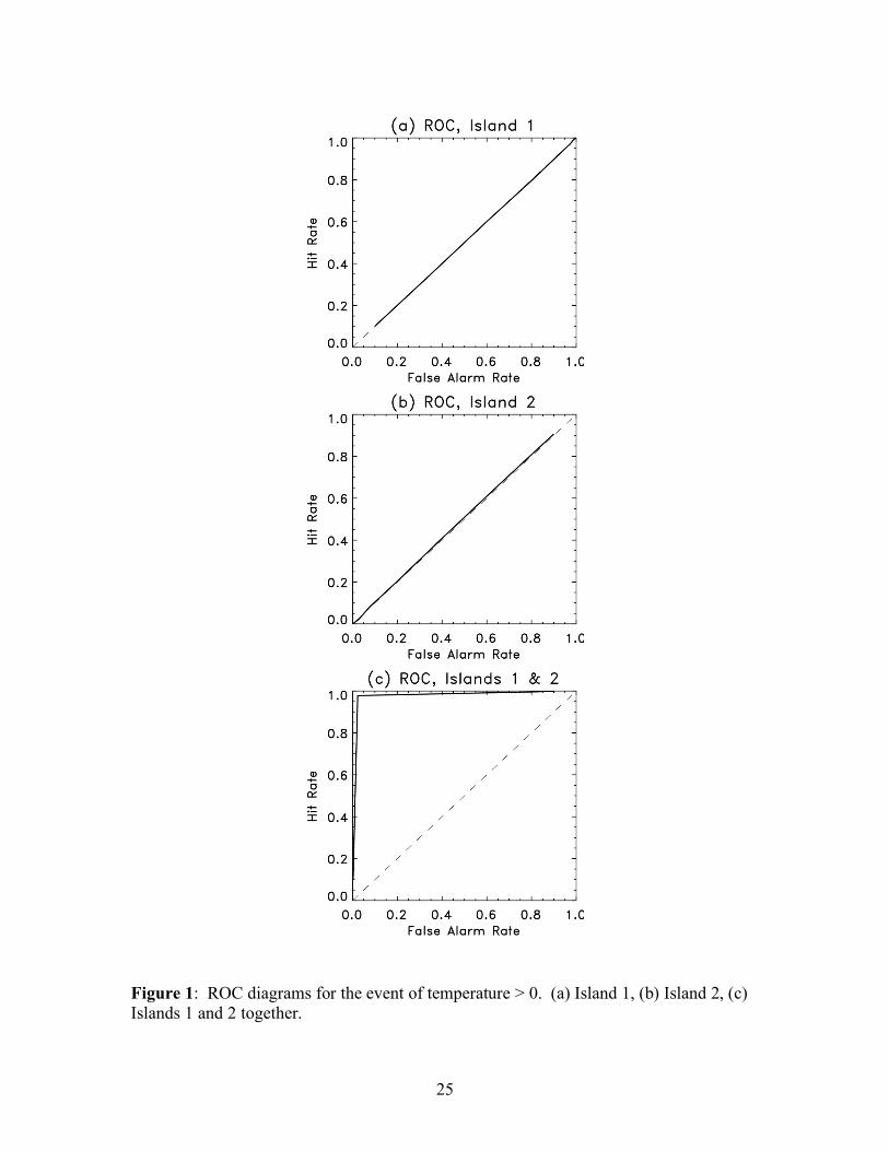
b. Relative operating characteristics

ROCs were generated for each island individually (Figs. 1 a–b) using (8) - (9),

and indeed, these each show no skill (area = 0.5). To generate one ROC over the two

islands, (10) – (11) were used. A ROC was then generated from the pooled tables (Fig.

1c). Note the very large positive area under the ROC curve, suggesting nearly perfect

forecast skill.

Why was skill now indicated by the ROC? By compositing data over the two

islands, the ROC analysis no longer implicitly assumed that the climatological

distribution was ~ N(+2, 1) or ~ N(-2, 1). Rather, it assumed that the climatological

distribution was ~ 0.5 • N(+2, 1) +0.5 • N(-2, 1), a bimodal distribution. Further, the

contingency tables were populated consistent with the assumption that the forecast

12

perfectly predicted which mode of the distribution the verification lay in; when the

forecasts were drawn from the positive mode N(+2, 1), the observed states were also

drawn from the positive mode N(+2, 1), and when the forecasts were drawn from N(-2,

1), the observed state were drawn from N(-2, 1) as well. This can be demonstrated by

generating a ROC simulated under these assumptions. Such a ROC is identical to that in

Fig. 1c.

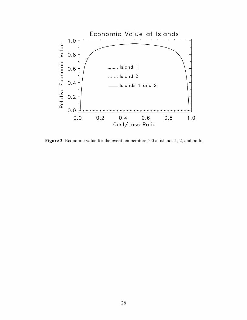
c. Economic value diagrams.

Figure 2 shows the economic value diagrams under the assumption that Lu = 0.

As with the ROCs, the economic value was nil when computed at the individual islands

using (16), but the diagram indicated that when averaged contingency tables and (18) –

(20) were used, near-perfect economic value was realized at moderate cost/loss ratios.

The underlying explanation is the same as for the ROC, the redefinition of climatology

from the inappropriate compositing of contingency table elements.

4. 850 hPa temperature

Consider whether or not false skill can be reported with real data. 0000 UTC 850

hPa temperature analyses were extracted from the NCEP-NCAR reanalysis at a set of

26x12 grid points covering the conterminous United States (US). Data was considered

for the first 60 days of 1979 to 2001. The grid spacing was 2.5° in latitude and

longitude. Let T denote the temperature at a grid point, and T ’ denote the temperature

anomaly from the mean. Three events were considered: (1) T > 0C, (2) T ’ > 3C, and (3)

13

T ’ > Q 2/3, where Q 2/3 was the upper tercile of the climatological distribution, i.e., the

temperature threshold defining the boundary between the lower two-thirds of the

distribution and the upper third. Q 2/3 was specified uniquely for each grid point.

First the method for generating contingency tables for the event T > 0C is

described. For each of the first 60 days of the year and for each of the 23 years (1380

samples), the following process was performed at each grid point: (1) the analyzed

temperature was extracted at that grid point, (2) a cross-validated, 50-member ensemble

was randomly drawn from the climatology of that grid point, excluding draws from the

year being processed, (3) the ensemble was sorted, and (4) contingency tables were

populated for that grid point, and (5) average contingency tables for all of the grid points

were also generated.

When generating ROCs for the events T ’ > 3C, and T ’ > Q 2/3, several additional

steps were required. After step (1) above, the climatological mean for each date and

location was determined and subtracted from the temperature, creating a database of

temperature anomalies. The estimated climatological mean was estimated using a 30-day

window centered on each day and cross-validated by year, using the remaining 22 years.

Also, the terciles of the distribution were determined for each grid point.

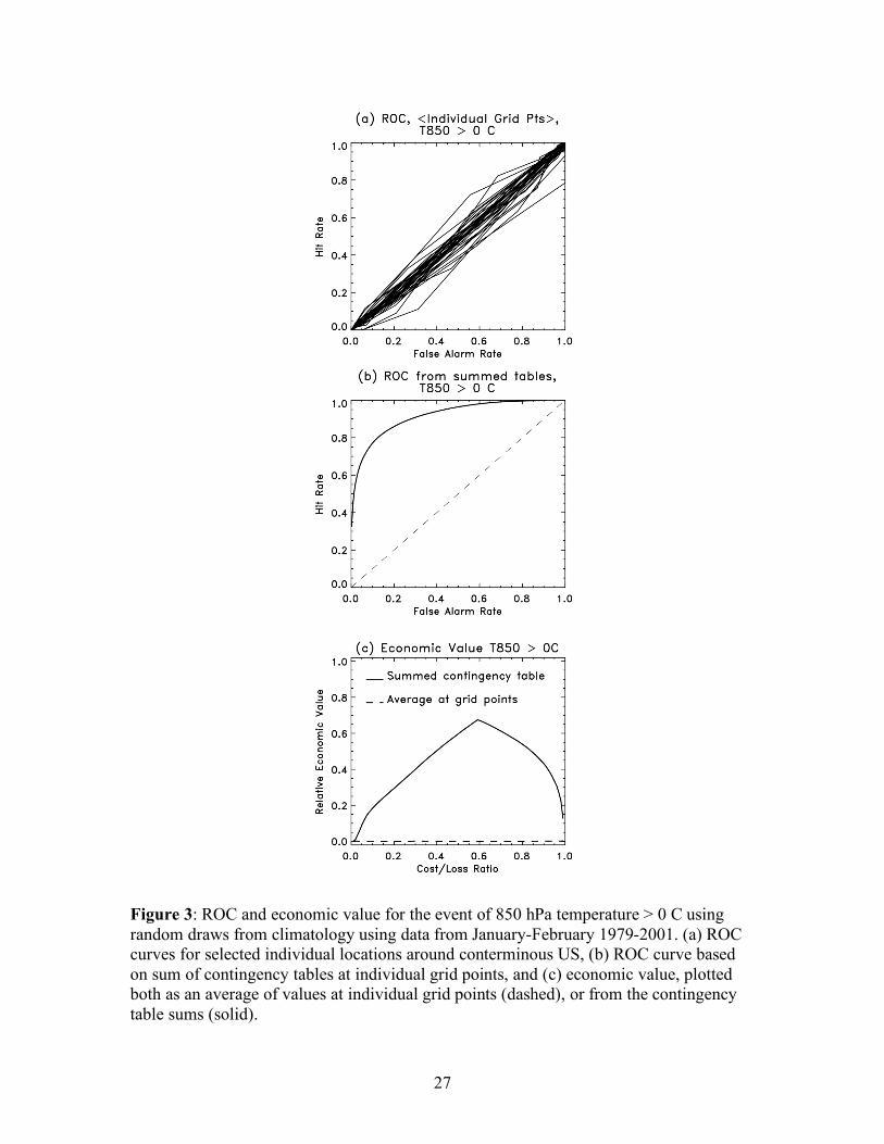
a. T > 0 C

When a location-dependent reference climatology is used (eqs. 4-5), the BSS is -

0.03. When a domain-averaged climatology is used (eqs. 6-7), the BSS reports a false

skill of +0.52.

14

Figure 3a shows ROCs calculated from the individual grid point data; the ROC

for every third grid point in the N-S and E-W directions are plotted. The ROCs exhibit

sampling variability but lie close to the HR=FAR line. However, the ROC based on a

contingency table summed up over all the grid points (Fig. 3b) diagnose a very large

amount of skill. Figure 3c shows that when the economic value is calculated separately

at each grid point and then averaged, its value is effectively zero. However, the

economic value calculated from the contingency table sums is large. Again, these are

artifacts of the widely differing climatologies for the grid points, as in section 2. In this

application, grid points in the north of the domain will almost always have 850 hPa

temperatures < 0, while this rarely happens at the southernmost grid points.

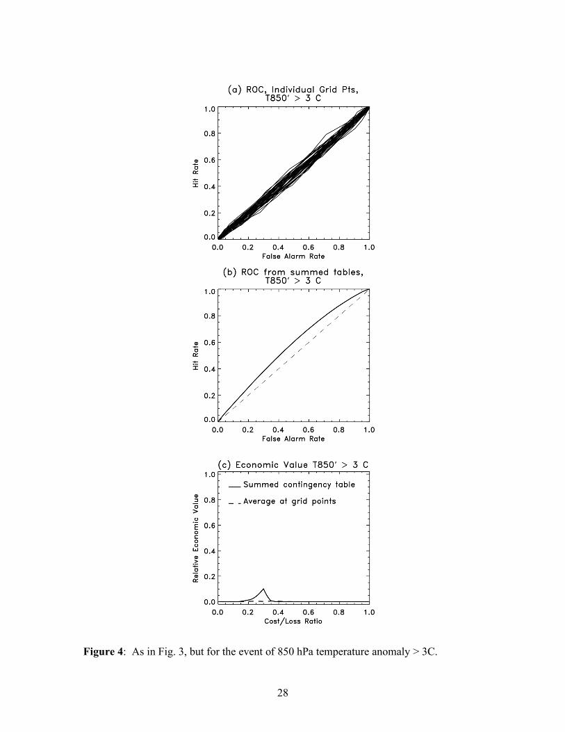
b. T ’ > 3 C

Considering events defined by anomalies of temperature rather than temperature

itself, the ensemble should have a much more consistent climatology from grid point to

grid point. However, at the southernmost, more tropically influenced grid points, a

deviation of 3C represented a relatively large deviation from climatology, while at the

northernmost grid points, 3C was smaller. The climatological probability of exceeding

this ranged from 0.45 in the north to 0.06 in the south.

When the location-dependent reference climatology was used, the reported BSS

was -0.03. When the domain-averaged climatology was used, the BSS was

-0.002. The extra skill when testing deviations from climatology was much less than

when the fixed threshold was tested in the previous example.

15

Figures 4 a-b show the ROCs for individual grid points and from the summed

contingency tables, respectively, and Fig. 4c shows the economic values as in Fig. 3c.

The area under the ROC curve was much reduced but was still greater than the expected

0.5. The economic value from the contingency table sums still reported unrealistic

positive value at cost-loss ratios around 0.3, but they were much smaller.

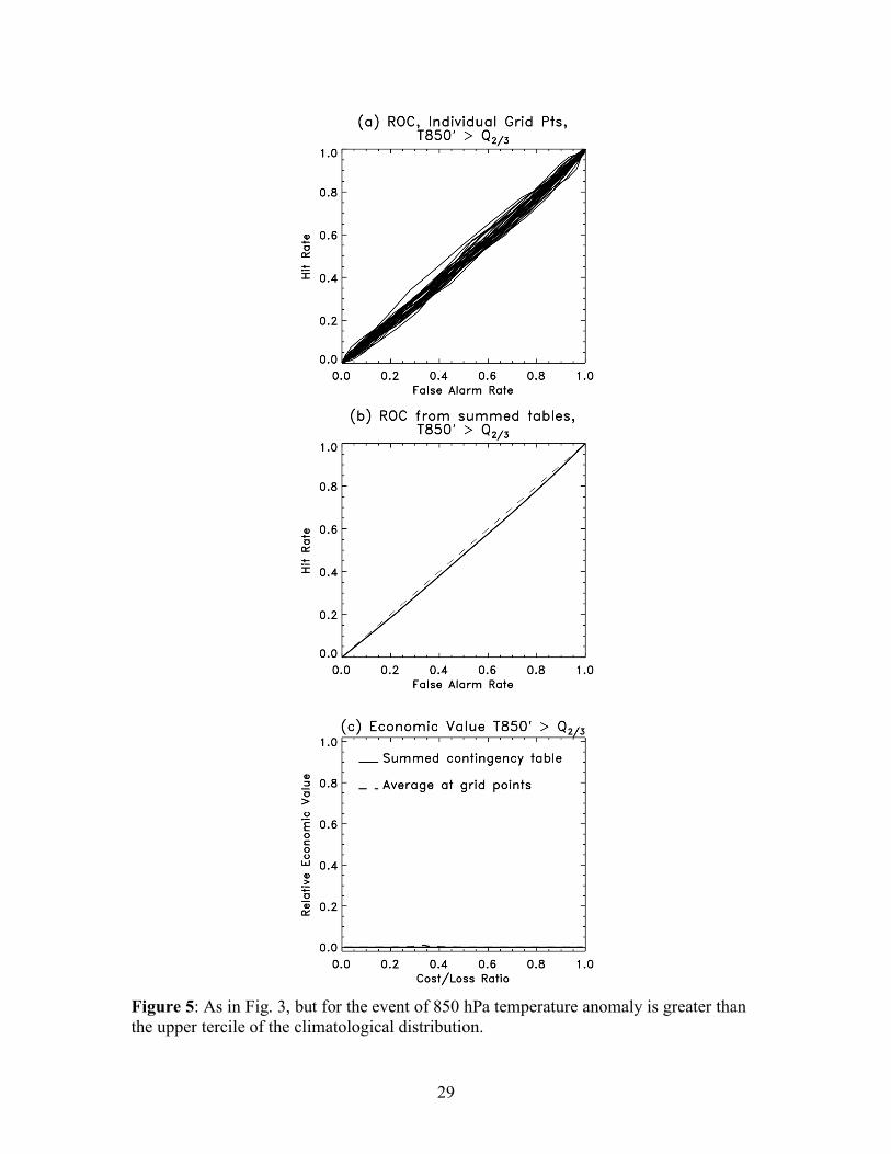
c. T ’ > Q 2/3

By evaluating the probability of exceeding a quantile of the distribution, the

climatological probabilities have been rendered uniform across all grid points; the

climatology probability is of course 1/3 for this event. By construction, the BSS is the

same for both, -0.03 (it is less than zero because the 50-member random draw from

climatology only approximates the true climatology). With ROCs and economic values,

whether we examined the average of scores at the grid points or computed the scores

from contingency table sums, we found no skill (Fig. 5).

4. Discussion

The preceding examples have demonstrated that the Brier skill score, relative

operating characteristic, and economic value diagrams must be used with care when

verifying probabilistic weather forecasts. Typically, the meteorological question being

asked is something akin to “what is the general skill of my forecast averaged over

Europe?” The naïve approach for calculating the Brier skill score may be to compute it

under the assumption that the climatology is invariant across the verification region.

Similarly, when diagnosing the relative operating characteristic or economic value, a

16

common step is to composite the forecast data into contingency tables that accumulate

weather information across the domain. The preceding analysis showed that these

diagnostics may falsely report positive skill in situations where the climatology differs

across the domain. The more the climatology differs, the larger the falsely reported skill.

By logical extension, false skill may also be reported if the climatology from compositing

samples from different seasons.

Several implications can be made about ensemble verification:

• Many prior studies, including one by the lead author, should be re-

evaluated, for the reported skill may be erroneous.

• In order to avoid reporting false skill, the researcher can alter his or her

verification methodology. Alternative methodologies can be used that should not

report false skill, such as: (1) analyze events where the climatological

probabilities are the same throughout the sample. Section 4 demonstrated that, for

example, ROCs and economic value diagrams of climatological forecasts of

quantiles of the 850 hPa temperature distribution did not report false positive

skill. Regardless of whether the climatological means and variances are large or

small, the fraction events classified as “yes” events are identical for different

locations or times of the year. (2) If sample sizes are large enough, perform the

calculations separately each for subsample with a different climatology. The data

could then be summarized in some manner; perhaps with a histogram of ROC

area for each of the subsamples, a map of the skill scores at individual grid points

with differing climatologies (e.g. Hamill and Whitaker 2005, Fig. 7), or an

average of economic value curves at individual grid points.

17

• Other scores such as the ranked probability skill score (Wilks 1995) can

also falsely report positive skill, just as with the Brier skill score. Whatever the

chosen verification metric, it is wise to verify that climatological forecasts give

the expected no-skill result before proceeding.

• Richardson (2001) demonstrated in a carefully controlled experiment

that there was a theoretical equivalence between the Brier skill score and the

integral of economic value assuming that users have a uniform distribution of

cost-loss ratios between 0 and 1. One of the underlying assumptions was an

invariant climatology across all samples. If this assumption is not met, then

neither is this equivalence.

Acknowledgments

Dan Wilks and William M. (“Matt”) Briggs (Cornell University), and Jeff Whitaker

(NOAA/CDC) are thanked for their discussions and comments on an early version of this

manuscript. This research was supported by National Science Foundation grants ATM-

0130154 and ATM-0205612.

18

References

Brier, G. W., 1950: Verification of forecasts expressed in terms of probabilities. Mon.

Wea. Rev., 78, 1-3.

Bright, D. R., and S. L. Mullen, 2002: Short-range ensemble forecasts of precipitation

during the southwest monsoon. Wea. Forecasting, 17, 1080–1100.

Buizza, R., and T. N. Palmer. 1998: Impact of ensemble size on ensemble prediction.

Mon. Wea. Rev., 126, 2503–2518.

----------, A. Hollingsworth, F. Lalaurette, and A. Ghelli, 1999: Probabilistic predictions

of precipitation using the ECMWF ensemble prediction system. Wea.

Forecasting, 14, 168-189.

----------, --------- , ---------, and --------, 2000: Reply to comments by Wilson and by

Juras. Wea. Forecasting, 15, 367-369.

----------, D. S. Richardson, and T. N. Palmer, 2003: Benefits of increased resolution in

the ECMWF ensemble prediction system and comparison with poor-man’s

ensembles. Quart. J. Royal Meteor. Soc., 129, 1269-1288.

Epstein, E. S., 1969: A scoring system for probability forecasts of ranked categories. J.

Appl. Meteor., 8, 190-198.

Gallus, W. A., Jr., and M. Segal, 2004: Does increased predicted warm-season rainfall

indicate enhanced likelihood of rain occurrence? Wea. Forecasting, 19, 1127–

1135.

19

Hamill, T. M., C. Snyder, D. P. Baumhefner, Z. Toth, and S. L. Mullen, 2000a: Ensemble

forecasting in the short to medium range: report from a workshop. Bull. Amer.

Meteor. Soc., 81, 2653-2664.

------------ , ------------- , and R. E. Morss, 2000: A comparison of probabilistic forecast

from bred, singular vector and perturbed observation ensembles. Mon. Wea. Rev.,

128, 1835-1851.

------------ , and J. S. Whitaker, 2005: Reforecasts, an important new data set for

improving weather predictions. Bull. Amer. Meteor. Soc., submitted. Available

at http://www.cdc.noaa.gov/people/tom.hamill/reforecast_bams.pdf .

Harvey, L. O., Jr., K. R. Hammond, C. M. Lusk, and E. F. Mross, 1992: The application

of signal detection theory to weather forecasting behavior. Mon. Wea. Rev., 120,

863-883.

Juras, J., 2000: Comments on “probabilistic predictions of precipitation using the

ECMWF ensemble prediction system.” Wea. Forecasting, 15, 365-366.

Kharin, V. V., and F. W. Zwiers, 2003: On the ROC score of probability forecasts. J.

Climate, 16, 4145–4150.

Kheshgi, H. S., and B. S. White, 2001: Testing distributed parameter hypotheses for the

detection of climate change. J. Climate, 14, 3464–3481.

Legg, T. P., K. R. Mylne. 2004: Early warnings of severe weather from ensemble

forecast information. Wea. Forecasting, 19, 891–906.

Marzban, C. 2004: The ROC curve and its area under it as performance measures. Wea.

Forecasting, 19, 1106-1114.

20

Mason, I. 1982: A model for the assessment of weather forecasts. Aust. Meteor. Mag.,

30, 291-303.

Mason, S. J., and N. E. Graham, 1999: Conditional probabilities, relative operating

characteristics, and relative operating levels. Wea. Forecasting, 14, 713-725.

Mullen, S. L., and R. Buizza, 2001: Quantitative precipitation forecasts over the United

States by the ECMWF ensemble prediction system. Mon. Wea. Rev., 129, 638–

663.

-----------, and ----------, 2002: The impact of horizontal resolution and ensemble size on

probabilistic forecasts of precipitation by the ECMWF ensemble prediction

system. Wea. Forecasting, 17, 173–191.

Murphy, A. H., 1971: A note on the ranked probability score. J. Appl. Meteor., 10, 155-

156.

Palmer, T. N., C. Brankovic, and D. S. Richardson, 2000: A probability and decision-

model analysis of PROVOST seasonal multi-model ensemble integrations.

Quart. J. Royal Meteor. Soc., 126, 2013-2033.

Richardson, D. S. , 2000: Skill and relative economic value of the ECMWF ensemble

prediction system. Quart. J. Royal Meteor. Soc., 126, 649-667.

-----------, 2001a: Ensembles using multiple models and analyses. Quart. J. Royal

Meteor. Soc., 127, 1847-1864.

-----------, 2001b: Measures of skill and value of ensemble prediction systems, their

interrelationship and the effect of ensemble size. Quart. J. Royal Meteor. Soc.,

127, 2473-2489.

21

Swets, J. A., 1973: The relative operating characteristic in psychology. Science, 182,

990-999.

Stanski, H. R., L. J. Wilson, and W. R. Burrows, 1989. Survey of common verification

methods in meteorology. Enviroment Canada Research Report 89-5, 114 pp.

Available from Atmospheric Environment Service, Forecast Research Division,

4905 Dufferin St., Downsview, ON M3H 5T4, Canada.

Wandishin, M. S., S. L. Mullen, D. J. Stensrud, and H. E. Brooks. 2001: Evaluation of a

short-range multimodel ensemble system. Mon. Wea. Rev., 129, 729–747.

Wilks, D. S., 1995: Statistical Methods in the Atmospheric Sciences. Cambridge Press.

547 pp.

-----------, 2001: A skill score based on economic value for probability forecasts. Meteor.

Appl., 8, 209-219.

Wilson, L. J., 2000: Comments on “probabilistic predictions of precipitation using the

ECMWF ensemble prediction system.” Wea. Forecasting, 15, 361-364.

World Meteorological Organization, 1992: Manual on the Global Data Processing

System, section III, Attachment II.7 and II.8, (revised in 2002). Available from

http://www.wmo.int/web/www/DPS/Manual/WMO485.pdf.

Yang, Z., and R.W. Arritt, 2002: Tests of a perturbed physics ensemble approach for

regional climate modeling. J. Climate, 15, 2881–2896.

Zhu, Y., Z. Toth, R. Wobus, D. Richardson and K. R. Mylne. 2002: The economic value

of ensemble-based weather forecasts. Bull. Amer. Meteor. Soc., 83, 73–83.

22

LIST OF TABLES Table 1: Contingency table for the ith of the n sorted members at the jth location,

indicating the relative fraction of hits [ai(j)], misses [bi(j)], false alarms [ci(j)], and correct

rejections [di(j)]. The economic costs associated with each contingency are also shown

and are discussed in the text.

23

LIST OF FIGURES Figure 1: ROC diagrams for the event of temperature > 0. (a) Island 1, (b) Island 2, (c)

Islands 1 and 2 together.

Figure 2: Economic value for the event temperature > 0 at islands 1, 2, and both.

Figure 3: ROC and economic value for the event of 850 hPa temperature > 0 C using

random draws from climatology using data from January-February 1979-2001. (a) ROC

curves for selected individual locations around conterminous US, (b) ROC curve based

on sum of contingency tables at individual grid points, and (c) economic value, plotted

both as an average of values at individual grid points (dashed), or from the contingency

table sums (solid).

Figure 4: As in Fig. 3, but for the event of 850 hPa temperature anomaly > 3C.

Figure 5: As in Fig. 3, but for the event of 850 hPa temperature anomaly is greater than

the upper tercile of the climatological distribution.

24

Event forecast by ith member?

YES NO ------------------------------------------------------------------------ YES | ai (j) | bi (j) | Event | Mitigated loss (C+Lu) | Loss (L = Lp + Lu) | Observed? |---------------------------------- | ---------------------------------- | NO | ci (j) | di (j) | | Cost (C) | No cost | ------------------------------------------------------------------------ Table 1: Contingency table for the ith of the n sorted members at the jth location, indicating the relative fraction of hits [ai(j)], misses [bi(j)], false alarms [ci(j)], and correct rejections [di(j)]. The economic costs associated with each contingency are also shown and are discussed in the text.

25

Figure 1: ROC diagrams for the event of temperature > 0. (a) Island 1, (b) Island 2, (c) Islands 1 and 2 together.

26

Figure 2: Economic value for the event temperature > 0 at islands 1, 2, and both.

27

Figure 3: ROC and economic value for the event of 850 hPa temperature > 0 C using random draws from climatology using data from January-February 1979-2001. (a) ROC curves for selected individual locations around conterminous US, (b) ROC curve based on sum of contingency tables at individual grid points, and (c) economic value, plotted both as an average of values at individual grid points (dashed), or from the contingency table sums (solid).

28

Figure 4: As in Fig. 3, but for the event of 850 hPa temperature anomaly > 3C.

29

Figure 5: As in Fig. 3, but for the event of 850 hPa temperature anomaly is greater than the upper tercile of the climatological distribution.