Embed Size (px)
Citation preview

BASIC CONCEPTS
AND
CONVENTIONAL METHODS
OF
STUCTURAL ANALYSIS (LECTURE NOTES)
DR. MOHAN KALANI (Retired Professor of Structural Engineering)
DEPARTMENT OF CIVIL ENGINEERING
INDIAN INSTITUTE OF TECHNOLOGY (BOMBAY) POWAI, MUMBAI – 400 076, INDIA
WWW.ENGGROOM.COM DOWNLOADED FROM WWW.ENGGROOM.COM
FOR MORE STUDY MATERIALS AND PROJECT VISIT WWW.ENGGROOM.COM

ACKNOWLEDGEMENTS
I realize the profound truth that He who created all things inert as well as live is
GOD. But many things in this world are created through knowledge of some living
beings and these living beings are groomed by their teachers and through their own effort
of self study and practice.
Those who are gifted by God are exceptions and those who are gifted by their
teachers are lucky. I am thankful to God as He has been grateful to me much more than I
deserve and to my all teachers from school level to University heights as I am product of
their efforts and guidance and hence this work.
It is not out of place to mention some names that did excellent job of teaching and
showed path to learning, teaching and research. Mr. Sainani of Baba Thakurdas Higher
Secondary School, Lucknow, India did excellent job of teaching of mathematics at school
level. Mr. Tewarson of Lucknow Christian College, Lucknow, India was an excellent
teacher of mathematics at college level. Professor Ramamurty taught theory of Structures
excellently at I.I.T. Kharagpur, India. Visiting Professor Paul Andersen from U.S.A.
demonstrated the techniques of teaching through his very well prepared lectures and
course material on Structural Mechanics, Soil Mechanics and his consultancy practice.
Visiting Professor Gerald Picket taught Advanced Theory of Elasticity, Plates and shells.
It was a rare opportunity to be their student during Master of Engineering Course of
Calcutta University at Bengal Engineering College, Howrah, India.
During my Ph.D. programme at Leningrad Plytechnic Institute, Leningrad (St.
Petersberg), Russia, Professor L.A. Rozin, Head of Department of Structural Mechanics
and Theory of Elasticity presented lectures and course material on Matrix Methods of
Finite Element Analysis excellently.
The present work is the result of inspirations of my teachers and also any future
work that I may accomplish.
Last but not the least, I express my gratitude to Professor Tarun Kant, Present
Dean (Planning) I.I.T. Powai, Mumbai India and Ex. Head of Civil Engineering
Department who extended the facility of putting this work on web site of I.I.T. Powai,
Mumbai, India. Also I thank present Head of Civil engineering Department, I.I.T. Powai,
India. Professor G.Venkatachalam who whole heatedly extended the facility of typing
this manuscript in the departmental library by Mrs. Jyoti Bhatia and preparation of
figures in the drawing office by Mr. A.J. Jadhav and Mr. A.A. Hurzuk.
Above all I am thankful to Professor Ashok Misra, Director of I.I.T. Powai,
Mumbai, India who has a visionary approach in the matters of theoretical and practical
development of knowledge hence, the I.I.T. employees in service or retired get the
appropriate support from him in such matters. He has the plans to make I.I.T. Powai the
best institute in the world.
WWW.ENGGROOM.COM DOWNLOADED FROM WWW.ENGGROOM.COM
FOR MORE STUDY MATERIALS AND PROJECT VISIT WWW.ENGGROOM.COM

The inspiration and knowledge gained from my teachers and literature have
motivated me to condense the conventional methods of structural analysis in this work so
that a reader can get the quick insight into the essence of the subject of Structural
Mechanics.
In the end I wish to acknowledge specifically the efforts of Mrs. Jyoti Bhatia, who
faithfully, sincerely and conscientiously typed the manuscript and perfected it as far as
possible by reviewing and removing the errors.
Finally I thank Sri Anil Kumar Sahu who scanned all the figures and integrated
the same with the text and arranged the entire course material page wise.
WWW.ENGGROOM.COM DOWNLOADED FROM WWW.ENGGROOM.COM
FOR MORE STUDY MATERIALS AND PROJECT VISIT WWW.ENGGROOM.COM

REFERENCES
1. Andersen P. Statically Indeterminate Structures. The Ronald Press Company, New
York, U.S.A, 1953.
2. Darkov A & Kuznetsov V. Structural Mechanics. Mir Publishers, Moscow, Russia.
3. Junnarkar S.B. Mechanics of Structures, Valumes I & II. Chartor Book Stall, Anand,
India.
4. Mohan Kalani. Analysis of continuous beams and frames with bars of variable cross-
section. I. Indian Concrete Journal, March 1971.
5. Mohan Kalani. Analysis of continuous beams and frames with bars of variable cross-
section :2. Indian Concrete Journal, November 1971.
6. Norris C.H., Wilbur J.B & Utku S. Elementary Structural Analysis. McGraw – Hill
Book Company, Singapore.
7. Raz Sarwar Alam. Analytical Methods in Structural Engineering. Wiley Eastern
Private Limited, New Delhi, India.
8. Timoshenko S.P & Young D.H. Theory of Structures. McGraw – Hill Kogakusha
Ltd., Tokyo, Japan.
9. Vazirani V.N. & Ratwani M.M. Analysis of Structures, Khanna Publishers, Delhi,
India.
10. West H.H. Analysis of Structures. John Wiley & Sons, New York, USA.
WWW.ENGGROOM.COM DOWNLOADED FROM WWW.ENGGROOM.COM
FOR MORE STUDY MATERIALS AND PROJECT VISIT WWW.ENGGROOM.COM

CONTENTS
CHAPTER TOPIC PAGE NO
1. INTRODUCTION 1
2. CLASSIFICATION OF SKELEAL
OR FRAMED STRUCTURES 1
3. INTERNAL LOADS DEVELOPED IN
STRUCTURAL MEMBERS 2
4. TYPES OF STRUCTURAL LOADS 3
5. DTERMINATE AND INDETERMINATE 4
STRUCTURAL SYSTEMS
6. INDETERMINACY OF STRUCTURAL SYSTEM 7
7. FLEXIBILITY AND STIFFNESS METHODS 11
8. ANALYSIS OF STATICALLY DETERMINATE
STRUCTURES 12
9. ANALYSIS OF DETERMINATE TRUSSES 16
10. CABLES AND ARCHES 25
11. INFLUENCE LINES FOR DETERMINATE
STRUCTURES 32
12. DEFLECTION OF STRUCTURES 37
13. NONPRISMATIC MEMBERS 49
14. SLOPE DEFLECTION EQUATIONS 54
15. MOMENT DISTRIBUTION METHOD 58
WWW.ENGGROOM.COM DOWNLOADED FROM WWW.ENGGROOM.COM
FOR MORE STUDY MATERIALS AND PROJECT VISIT WWW.ENGGROOM.COM

16. ANALYSIS OF CONTINUOUS BEAMS AND
PLANE FRAMES CONSISTING OF PRISMATIC
AND NONPRISMATIC MEMBERS 69
17. ANALYSIS OF INDETERMINATE TRUSSES 79
18. APPROXIMATE METHODS OF ANALYSIS OF
STATICALLY INDETERMINATE STRUCTURES 89
WWW.ENGGROOM.COM DOWNLOADED FROM WWW.ENGGROOM.COM
FOR MORE STUDY MATERIALS AND PROJECT VISIT WWW.ENGGROOM.COM

LECTURE NOTES ON STRUCTURAL ANALYSIS
BY DR. MOHAN KALANI
RETIRED PROFESSOR OF STRUCTURAL ENGINEERING
CIVIL ENGINEERING DEPARTMENT
INDIAN INSTITUTE OF TECHNOLOGY,
MUMBAI-400 076, INDIA
BASIC CONCEPTS AND CONVENTIONAL METHODS OF STRUCTURAL
ANALYSIS
1 INTRODUCTION
The structural analysis is a mathematical algorithm process by which the response of a
structure to specified loads and actions is determined. This response is measured by
determining the internal forces or stress resultants and displacements or deformations
throughout the structure.
The structural analysis is based on engineering mechanics, mechanics of solids,
laboratory research, model and prototype testing, experience and engineering judgment.
The basic methods of structural analysis are flexibility and stiffness methods. The
flexibility method is also called force method and compatibility method. The stiffness
method is also called displacement method and equilibrium method. These methods are
applicable to all type of structures; however, here only skeletal systems or framed
structures will be discussed. The examples of such structures are beams, arches, cables,
plane trusses, space trusses, plane frames, plane grids and space frames.
The skeletal structure is one whose members can be represented by lines possessing
certain rigidity properties. These one dimensional members are also called bar members
because their cross sectional dimensions are small in comparison to their lengths. The
skeletal structures may be determinate or indeterminate.
2 CLASSIFICATIONS OF SKELETAL OR FRAMED STRUCTURES
They are classified as under.
1) Direct force structures such as pin jointed plane frames and ball jointed space
frames which are loaded and supported at the nodes. Only one internal force or
stress resultant that is axial force may arise. Loads can be applied directly on the
members also but they are replaced by equivalent nodal loads. In the loaded
members additional internal forces such as bending moments, axial forces and
shears are produced.
The plane truss is formed by taking basic triangle comprising of three members and three
pin joints and then adding two members and a pin node as shown in Figure 2.1. Sign
WWW.ENGGROOM.COM DOWNLOADED FROM WWW.ENGGROOM.COM
FOR MORE STUDY MATERIALS AND PROJECT VISIT WWW.ENGGROOM.COM

WWW.ENGGROOM.COM DOWNLOADED FROM WWW.ENGGROOM.COM
FOR MORE STUDY MATERIALS AND PROJECT VISIT WWW.ENGGROOM.COM

WWW.ENGGROOM.COM DOWNLOADED FROM WWW.ENGGROOM.COM
FOR MORE STUDY MATERIALS AND PROJECT VISIT WWW.ENGGROOM.COM

WWW.ENGGROOM.COM DOWNLOADED FROM WWW.ENGGROOM.COM
FOR MORE STUDY MATERIALS AND PROJECT VISIT WWW.ENGGROOM.COM

WWW.ENGGROOM.COM DOWNLOADED FROM WWW.ENGGROOM.COM
FOR MORE STUDY MATERIALS AND PROJECT VISIT WWW.ENGGROOM.COM

-2-
Convention for internal axial force is also shown. In Fig.2.2, a plane triangulated truss
with joint and member loading is shown. The replacement of member loading by joint
loading is shown in Fig.2.3. Internal forces developed in members are also shown.
The space truss is formed by taking basic prism comprising of six members and four ball
joints and then adding three members and a node as shown in Fig.2.4.
2) Plane frames in which all the members and applied forces lie in same plane as
shown in Fig.2.5. The joints between members are generally rigid. The stress
resultants are axial force, bending moment and corresponding shear force as shown
in Fig.2.6.
3) Plane frames in which all the members lay in the same plane and all the applied
loads act normal to the plane of frame as shown in Fig.2.7. The internal stress
resultants at a point of the structure are bending moment, corresponding shear force
and torsion moment as shown in Fig.2.8.
4) Space frames where no limitations are imposed on the geometry or loading in
which maximum of six stress resultants may occur at any point of structure namely
three mutually perpendicular moments of which two are bending moments and one
torsion moment and three mutually perpendicular forces of which two are shear
forces and one axial force as shown in figures 2.9 and 2.10.
3 INTERNAL LOADS DEVELOPED IN STRUCTURAL MEMBERS
External forces including moments acting on a structure produce at any section along a
structural member certain internal forces including moments which are called stress
resultants because they are due to internal stresses developed in the material of member.
The maximum number of stress resultants that can occur at any section is six, the three
Orthogonal moments and three orthogonal forces. These may also be described as the
axial force F1 acting along x – axis of member, two bending moments F5 and F6 acting
about the principal y and z axes respectively of the cross section of the member, two
corresponding shear forces F3 and F2 acting along the principal z and y axes respectively
and lastly the torsion moment F4 acting about x – axis of member. The stress resultants at
any point of centroidal axis of member are shown in Fig. 3.1 and can be represented as
follows.
WWW.ENGGROOM.COM DOWNLOADED FROM WWW.ENGGROOM.COM
FOR MORE STUDY MATERIALS AND PROJECT VISIT WWW.ENGGROOM.COM

WWW.ENGGROOM.COM DOWNLOADED FROM WWW.ENGGROOM.COM
FOR MORE STUDY MATERIALS AND PROJECT VISIT WWW.ENGGROOM.COM

-3-
{ }
⎪⎪⎪⎪
⎭
⎪⎪⎪⎪
⎬
⎫
⎪⎪⎪⎪
⎩
⎪⎪⎪⎪
⎨
⎧
⎪⎪⎪⎪
⎭
⎪⎪⎪⎪
⎬
⎫
⎪⎪⎪⎪
⎩
⎪⎪⎪⎪
⎨
⎧
=
z
y
x
z
y
x
6
5
4
3
2
1
M
M
M
F
F
F
OR
F
F
F
F
F
F
F
Numbering system is convenient for matrix notation and use of electronic computer.
Each of these actions consists essentially of a pair of opposed actions which causes
deformation of an elemental length of a member. The pair of torsion moments cause twist
of the element, pair of bending moments cause bending of the element in corresponding
plane, the pair of axial loads cause axial deformation in longitudinal direction and the
pair of shearing forces cause shearing strains in the corresponding planes. The pairs of
biactions are shown in Fig.3.2.
Primary and secondary internal forces.
In many frames some of six internal actions contribute greatly to the elastic strain energy
and hence to the distortion of elements while others contribute negligible amount. The
material is assumed linearly elastic obeying Hooke’s law. In direct force structures axial
force is primary force, shears and bending moments are secondary. Axial force structures
do not have torsional resistance. The rigid jointed plane grid under normal loading has
bending moments and torsion moments as primary actions and axial forces and shears are
treated secondary.
In case of plane frame subjected to in plane loading only bending moment is primary
action, axial force and shear force are secondary. In curved members bending moment,
torsion and thrust (axial force) are primary while shear is secondary. In these particular
cases many a times secondary effects are not considered as it is unnecessary to
complicate the analysis by adopting general method.
4 TYPES OF STRUCTURAL LOADS
For the analysis of structures various loads to be considered are: dead load, live load,
snow load, rain load, wind load, impact load, vibration load, water current, centrifugal
force, longitudinal forces, lateral forces, buoyancy force, earth or soil pressure,
hydrostatic pressure, earthquake forces, thermal forces, erection forces, straining forces
etc. How to consider these loads is described in loading standards of various structures.
These loads are idealized for the purpose of analysis as follows.
WWW.ENGGROOM.COM DOWNLOADED FROM WWW.ENGGROOM.COM
FOR MORE STUDY MATERIALS AND PROJECT VISIT WWW.ENGGROOM.COM

-4-
Concentrated loads: They are applied over a small area and are idealized as point loads.
Line loads: They are distributed along narrow strip of structure such as the wall load or
the self weight of member. Neglecting width, load is considered as line load acting along
axis of member.
Surface loads: They are distributed over an area. Loads may be static or dynamic,
stationary or moving. Mathematically we have point loads and concentrated moments.
We have distributed forces and moments, we have straining and temperature variation
forces.
5 DETERMINATE AND INDETERMINATE STRUCTURAL SYSTEMS
If skeletal structure is subjected to gradually increasing loads, without distorting the
initial geometry of structure, that is, causing small displacements, the structure is said to
be stable. Dynamic loads and buckling or instability of structural system are not
considered here. If for the stable structure it is possible to find the internal forces in all
the members constituting the structure and supporting reactions at all the supports
provided from statical equations of equilibrium only, the structure is said to be
determinate. If it is possible to determine all the support reactions from equations of
equilibrium alone the structure is said to be externally determinate else externally
indeterminate. If structure is externally determinate but it is not possible to determine all
internal forces then structure is said to be internally indeterminate. Therefore a structural
system may be:
(1) Externally indeterminate but internally determinate
(2) Externally determinate but internally indeterminate
(3) Externally and internally indeterminate
(4) Externally and internally determinate
These systems are shown in figures 5.1 to 5.4.
A system which is externally and internally determinate is said to be determinate system.
A system which is externally or internally or externally and internally indeterminate is
said to be indeterminate system.
Let: v = Total number of unknown internal and support reactions
s = Total number of independent statical equations of equilibrium.
WWW.ENGGROOM.COM DOWNLOADED FROM WWW.ENGGROOM.COM
FOR MORE STUDY MATERIALS AND PROJECT VISIT WWW.ENGGROOM.COM

WWW.ENGGROOM.COM DOWNLOADED FROM WWW.ENGGROOM.COM
FOR MORE STUDY MATERIALS AND PROJECT VISIT WWW.ENGGROOM.COM

-5-
Then if: v = s the structure is determinate
v > s the structure is indeterminate
v < s the structure is unstable
Total indeterminacy of structure = Internal indeterminacy + External indeterminacy
Equations of equilibrium
Space frames arbitrarily loaded
∑Fx = 0 ∑Mx = 0
∑Fy = 0 ∑My = 0
∑Fz = 0 ∑Mz = 0
For space frames number of equations of equilibrium is 6. Forces along three orthogonal
axes should vanish and moments about three orthogonal axes should vanish.
Plane frames with in plane loading
∑Fx = 0 ∑Fy = 0 ∑Mz = 0
There are three equations of equilibrium. Forces in x and y directions should vanish and
moment about z axis should vanish.
Plane frames with normal to plane loading
There are three equations of equilibrium.
∑Fy = 0, ∑Mx = 0, ∑Mz = 0
Sum of forces in y direction should be zero. Sum of moments about x and z axes be zero.
Release and constraint
A release is a discontinuity which renders a member incapable of transmitting a stress
resultant across that section. There are six releases corresponding to the six stress
resultants at a section as shown below by zero elements in the vectors. Various releases
are shown in figures 5.5 to 5.12.
WWW.ENGGROOM.COM DOWNLOADED FROM WWW.ENGGROOM.COM
FOR MORE STUDY MATERIALS AND PROJECT VISIT WWW.ENGGROOM.COM

-6-
Release for Axial Force (AF) Fx:
⎪⎪⎪⎪
⎭
⎪⎪⎪⎪
⎬
⎫
⎪⎪⎪⎪
⎩
⎪⎪⎪⎪
⎨
⎧
z
y
x
z
y
M
M
M
F
F
0
Release for Shear Force (SF) Fy:
⎪⎪⎪⎪
⎭
⎪⎪⎪⎪
⎬
⎫
⎪⎪⎪⎪
⎩
⎪⎪⎪⎪
⎨
⎧
z
y
x
z
x
M
M
M
F
0
F
Release for Shear Force (SF) Fz:
⎪⎪⎪⎪
⎭
⎪⎪⎪⎪
⎬
⎫
⎪⎪⎪⎪
⎩
⎪⎪⎪⎪
⎨
⎧
z
y
x
y
x
M
M
M
0
F
F
Release for Torsion Moment (TM) Mx:
⎪⎪⎪⎪
⎭
⎪⎪⎪⎪
⎬
⎫
⎪⎪⎪⎪
⎩
⎪⎪⎪⎪
⎨
⎧
z
y
z
y
x
M
M
0
F
F
F
WWW.ENGGROOM.COM DOWNLOADED FROM WWW.ENGGROOM.COM
FOR MORE STUDY MATERIALS AND PROJECT VISIT WWW.ENGGROOM.COM

-7-
Release for Bending Moment (BM) My:
⎪⎪⎪⎪
⎭
⎪⎪⎪⎪
⎬
⎫
⎪⎪⎪⎪
⎩
⎪⎪⎪⎪
⎨
⎧
z
x
z
y
x
M
0
M
F
F
F
Release for Bending Moment (BM) Mz:
⎪⎪⎪⎪
⎭
⎪⎪⎪⎪
⎬
⎫
⎪⎪⎪⎪
⎩
⎪⎪⎪⎪
⎨
⎧
0
M
M
F
F
F
y
x
z
y
x
The release may be represented by zero elements of forces
Universal joint (Ball and socket joint) F =
⎪⎪⎪⎪
⎭
⎪⎪⎪⎪
⎬
⎫
⎪⎪⎪⎪
⎩
⎪⎪⎪⎪
⎨
⎧
0
0
0
F
F
F
z
y
x
, Cut F =
⎪⎪⎪⎪
⎭
⎪⎪⎪⎪
⎬
⎫
⎪⎪⎪⎪
⎩
⎪⎪⎪⎪
⎨
⎧
0
0
0
0
0
0
A release does not necessarily occur at a point, but may be continuous along whole length
of member as in chain for BM. On the other hand a constraint is defined as that which
prevents any relative degree of freedom between two adjacent nodes connected by a
member or when a relative displacement of the nodes does not produce a stress resultant
in the member.
6 INDETERMINACY OF STRUCTURAL SYSTEM
The indeterminacy of a structure is measured as statical (∝ s) or kinematical (∝ k)
indeterminacy.
∝ s = P (M – N + 1) – r = PR – r
∝ k = P (N – 1) + r – c
WWW.ENGGROOM.COM DOWNLOADED FROM WWW.ENGGROOM.COM
FOR MORE STUDY MATERIALS AND PROJECT VISIT WWW.ENGGROOM.COM
-8-
∝ s + ∝ k = PM –c
P = 6 for space frames subjected to general loading
P = 3 for plane frames subjected to in plane or normal to plane loading.
N = Number of nodes in structural system.
M = Number of members of completely stiff structure which includes foundation as
singly connected system of members. In completely stiff structure there is no release
present. In singly connected system of rigid foundation members there is only one route
between any two points in which tracks are not retraced. The system is considered
comprising of closed rings or loops.
R = Number of loops or rings in completely stiff structure.
r = Number of releases in the system.
c = Number of constraints in the system.
R = (M – N + 1)
For plane and space trusses ∝ s reduces to:
∝ s = M - (NDOF) N + P
M = Number of members in completely stiff truss.
P = 6 and 3 for space and plane truss respectively
N = Number of nodes in truss.
NDOF = Degrees of freedom at node which is 2 for plane truss and 3 for space truss.
For space truss ∝ s = M - 3 N + 6
For plane truss ∝ s = M - 2 N + 3
Test for static indeterminacy of structural system
If ∝ s > 0 Structure is statically indeterminate
If ∝ s = 0 Structure is statically determinate
WWW.ENGGROOM.COM DOWNLOADED FROM WWW.ENGGROOM.COM
FOR MORE STUDY MATERIALS AND PROJECT VISIT WWW.ENGGROOM.COM

-9-
and if ∝ s < 0 Structure is a mechanism.
It may be noted that structure may be mechanism even if ∝ s > 0 if the releases are
present in such a way so as to cause collapse as mechanism. The situation of mechanism
is unacceptable.
Statical Indeterminacy
It is difference of the unknown forces (internal forces plus external reactions) and the
equations of equilibrium.
Kinematic Indeterminacy
It is the number of possible relative displacements of the nodes in the directions of stress
resultants.
Computation of static and kinematic indeterminacies
It is possible to compute mentally the static and kinematic inderminacies of structures.
Consider a portal frame system shown in Fig.6.1. It is space structure with five members
and three clamps at foundation. There is one internal space hinge in member BC.
Foundation is replaced with two stiff members to give entire system as shown in Fig.6.2.
So we have completely stiff structure with seven members and forms two rings which are
statically indeterminate to twelve degrees as shown in Fig.6.3. There are three releases in
member BC because of ball and socket (universal) joint. Three moments are zero at this
section. Therefore ∝ s = 9. There are three joints E, B and C which can move. Being
space system degree of freedom per node is 6. There will be three rotations at universal
joint. Therefore total dof is (3 x 6 + 3) or ∝ k = 21. Joints F, A and D can not have any
displacement that is degree of freedom is zero at these nodes.
Using formula:
∝ s = P (M – N + 1) – r
∝ k = P (N – 1) + r – c
P = 6, M = 7, N = 6
c = 12 (Foundation members are rigid), r = 3
∝ s = P (M – N + 1) – r = 6 (7 – 6 + 1) – 3 = 9
∝ k = P (N – 1) + r – c = 6 (6 – 1) + 3 – 12 = 21
WWW.ENGGROOM.COM DOWNLOADED FROM WWW.ENGGROOM.COM
FOR MORE STUDY MATERIALS AND PROJECT VISIT WWW.ENGGROOM.COM

WWW.ENGGROOM.COM DOWNLOADED FROM WWW.ENGGROOM.COM
FOR MORE STUDY MATERIALS AND PROJECT VISIT WWW.ENGGROOM.COM

WWW.ENGGROOM.COM DOWNLOADED FROM WWW.ENGGROOM.COM
FOR MORE STUDY MATERIALS AND PROJECT VISIT WWW.ENGGROOM.COM

-10-
∝ s + ∝ k = PM – c = 6 x 7 – 12 = 30
Static indeterminacy can also be determined by introducing releases in the system and
rendering it a stable determinate system. The number of biactions corresponding to
releases will represent static indeterminacy. Consider a portal frame fixed at support
points as shown in Fig.6.4. The entire structure is shown in Fig.6.5 and completely stiff
structure in Fig.6.6.
∝ s = P (M – N + 1) – r
∝ k = P (N – 1) + r – c
P = 3, M = 4, N = 4, c = 3, r = 0
∝ s = 3 (4 – 4 + 1) – 0 = 3
∝ k = 3 (4 – 1) + 0 – 3 = 6
∝ s + ∝ k = 3 + 6 = 9
The structure can be made determinate by introducing in many ways three releases and
thus destroying its capacity to transmit internal forces X1, X2, X3 at the locations of
releases.
In figure 6.7. a cut is introduced just above clamp D that is clamp is removed. It becomes
tree or cantilever structure with clamp at A. At this cut member was transmitting three
forces X1, X2 and X3 (Two forces and one moment). Therefore ∝ s = 3. This is external
static indeterminacy.
In figure 6.8. a cut is introduced at point R on member BC. We have two trees or
cantilevers with clamps at A and D. We have three internal unknown forces X1, X2, and
X3. Thus ∝ s = 3.
In figure 6.9. three hinges are introduced. We have determinate and stable system and
there are three unknown moments X1, X2 and X3. Thus ∝ s = 3.
In figure 6.10. one roller cum hinge and one hinge is introduced. We have one unknown
force X1 and two unknown moments X2 and X3 at these releases. Thus ∝ s = 3.
The static and kinematic indeterminacies of a few structures are computed in Table 1.
WWW.ENGGROOM.COM DOWNLOADED FROM WWW.ENGGROOM.COM
FOR MORE STUDY MATERIALS AND PROJECT VISIT WWW.ENGGROOM.COM

WWW.ENGGROOM.COM DOWNLOADED FROM WWW.ENGGROOM.COM
FOR MORE STUDY MATERIALS AND PROJECT VISIT WWW.ENGGROOM.COM

WWW.ENGGROOM.COM DOWNLOADED FROM WWW.ENGGROOM.COM
FOR MORE STUDY MATERIALS AND PROJECT VISIT WWW.ENGGROOM.COM

-11-
TABLE 1. Examples on static and kinematic indeterminacies.
Example
No:
Figure
No:
P M N R c r ∝ s ∝ k
1 6.11 3 4 3 2 6 3 3 3
2 6.12 3 2 2 1 5 2 1 0
3 6.13 3 2 2 1 3 1 2 1
4 6.14 3 12 9 4 6 2 10 20
5 6.15 3 7 6 2 3 3 3 15
6 6.16 3 12 6 7 25 19 2 9
7 6.17 3 13 6 8 28 20 4 7
8 6.18 3 6
14
2
10
5
5
0
24
0
0
15
15
3
3
9 6.19 6 9 7 3 12 0 18 24
10 6.20 3 4 3 2 6 6 0 5
7 FLEXIBILITY AND STIFFNESS METHODS
These are the two basic methods by which an indeterminate skeletal structure is analyzed.
In these methods flexibility and stiffness properties of members are employed. These
methods have been developed in conventional and matrix forms. Here conventional
methods are discussed.
Flexibility Method
The given indeterminate structure is first made statically determinate by introducing
suitable number of releases. The number of releases required is equal to statical
indeterminacy ∝ s. Introduction of releases results in displacement discontinuities at these
releases under the externally applied loads. Pairs of unknown biactions (forces and
moments) are applied at these releases in order to restore the continuity or compatibility
of structure. The computation of these unknown biactions involves solution of linear
simultaneous equations. The number of these equations is equal to statical indeterminacy
∝ s. After the unknown biactions are computed all the internal forces can be computed in
the entire structure using equations of equilibrium and free bodies of members. The
required displacements can also be computed using methods of displacement
computation.
WWW.ENGGROOM.COM DOWNLOADED FROM WWW.ENGGROOM.COM
FOR MORE STUDY MATERIALS AND PROJECT VISIT WWW.ENGGROOM.COM

-12-
In flexibility method since unknowns are forces at the releases the method is also called
force method. Since computation of displacement is also required at releases for
imposing conditions of compatibility the method is also called compatibility method. In
computation of displacements use is made of flexibility properties, hence, the method is
also called flexibility method.
Stiffness Method
The given indeterminate structure is first made kinematically determinate by introducing
constraints at the nodes. The required number of constraints is equal to degrees of
freedom at the nodes that is kinematic indeterminacy ∝ k. The kinematically determinate
structure comprises of fixed ended members, hence, all nodal displacements are zero.
These results in stress resultant discontinuities at these nodes under the action of applied
loads or in other words the clamped joints are not in equilibrium. In order to restore the
equilibrium of stress resultants at the nodes the nodes are imparted suitable unknown
displacements. The number of simultaneous equations representing joint equilibrium of
forces is equal to kinematic indeterminacy ∝ k. Solution of these equations gives
unknown nodal displacements. Using stiffness properties of members the member end
forces are computed and hence the internal forces throughout the structure.
Since nodal displacements are unknowns, the method is also called displacement method.
Since equilibrium conditions are applied at the joints the method is also called
equilibrium method. Since stiffness properties of members are used the method is also
called stiffness method.
8 ANALYSIS OF STATICALLY DETERMINATE STRUCTURES
Following are the steps for analyzing statically determinate structures.
(1) Obtain the reactions at the supports of structure applying appropriate equations of
equilibrium.
(2) Separate the members at the joints as free bodies and apply equations of equilibrium
to each member to obtain member end forces.
(3) Cut the member at a section where internal forces are required. Apply equations of
equations to any of the two segments to compute unknown forces at this section.
Example 8.1
Compute reactions for the beam AB loaded as shown in figure 8.1. Also find internal
forces at mid span section C.
WWW.ENGGROOM.COM DOWNLOADED FROM WWW.ENGGROOM.COM
FOR MORE STUDY MATERIALS AND PROJECT VISIT WWW.ENGGROOM.COM

WWW.ENGGROOM.COM DOWNLOADED FROM WWW.ENGGROOM.COM
FOR MORE STUDY MATERIALS AND PROJECT VISIT WWW.ENGGROOM.COM

-13-
Detach the beam from supports and show unknown reactions as shown in Fig.8.2
The reaction RB which is perpendicular to rolling surface is replaced with its horizontal
and vertical components RBX and BBY.
RBX = RB Sin θ = 5
3 RB, RBY = RB Cos θ =
5
4 RB
At A reaction in vertical direction is zero and other components are RAX and MAZ.
Resultant of triangular load W is shown acting at 8m from A and 4m from B that is
through CG of triangular loading. The free body diagram with known forces is shown in
Fig.8.3.
W = 2
1 x 50 x 12 = 300 kN
The equations of equilibrium for the member are:
∑ Fx = 0, ∑ Fy = 0 and ∑ Mz = 0
Alternatively, ∑ Fx = 0, ∑A
zM = 0, ∑B
zM = 0
∑ Fx = 0 gives : RAX = RBX
∑ Fy = 0 gives : RBY = 300 kN
∑B
zM = 0 gives : MAZ = 4 x 300 = 1200 kNm
∑A
zM = 0 gives : 12 RBY = 8 x 300 + MAZ, RBY = 12
1200 2400 + = 300 (check)
RB = 4
5 x 300 = 375, RBX =
5
3 x 375 = 225.
Now the beam is cut at mid span and left segment is considered as a free body.
The free body diagram of segment AC with unknown forces is shown in Fig.8.4.
Total triangular load = 2
1 x 6 x 25 = 75 kN. It acts at 4m from A and 2m from C.
WWW.ENGGROOM.COM DOWNLOADED FROM WWW.ENGGROOM.COM
FOR MORE STUDY MATERIALS AND PROJECT VISIT WWW.ENGGROOM.COM
-14-
∑ Fx = 0 gives, RCX = 225 kN
∑ Fy = 0 gives, RCY = 75 kN
∑C
zM = 0 gives, MCZ = 1200 – 75 x 2 = 1050 kNm
Example 8.2
Determine the reactions for the three hinged arched frame ABC loaded as shown in Fig.
8.5. Show free body diagrams for members AB and BC and segments BD and DC.
We have three equations of equilibrium and four unknown reactions. The structure is
determinate despite four unknown reactions as the moment at hinge B is zero. The free
body diagrams of members AB and BC are shown in Fig.8.6 and Fig.8.7.
The equations of equilibrium of free body AB are
∑ Fx = 0, RAX – RBX = 0 ………. (1)
∑ Fy = 0, RAY + RBY = 40 ……… (2)
∑A
zM = 0, 3 RBX + 4 RBY = 40 x 2.5 = 100 ……… (3)
The equations of equilibrium of free body BC are :
∑ Fx = 0, RBX + RCX = 5 ………. (4)
∑ Fy = 0, - RBY + RCY = 10 ………. (5)
∑C
zM = 0, 4 RBX - 3 RBY = - 25 + 10 x 1.5 + 5 x 2 = 0 ……… (6)
These equations are solved for the unknown forces.
Eqn (3) x 4, 12 RBX + 16 RBY = 400 …….. (7)
Eqn (6) x 3, 12 RBX - 9 RBY = 0 ……... (8)
Eqn (7) – Eqn (8), 25 RBY = 400, RBY = 16
WWW.ENGGROOM.COM DOWNLOADED FROM WWW.ENGGROOM.COM
FOR MORE STUDY MATERIALS AND PROJECT VISIT WWW.ENGGROOM.COM

WWW.ENGGROOM.COM DOWNLOADED FROM WWW.ENGGROOM.COM
FOR MORE STUDY MATERIALS AND PROJECT VISIT WWW.ENGGROOM.COM

WWW.ENGGROOM.COM DOWNLOADED FROM WWW.ENGGROOM.COM
FOR MORE STUDY MATERIALS AND PROJECT VISIT WWW.ENGGROOM.COM

-15-
From (2), RAY = 40 – 16 = 24
From (7), RBX = 12
1 [400 – 16 x 16] =
12
144 = 12
From (8), RBX = 12
16 x 9 = 12 (check)
From (1), RAX = 12
From (4), RCX = 5 – 12 = - 7
From (5), RCY = 10 + 16 = 26
The free body diagrams of members AB and BC with known forces are shown in Figures
8.8 and 8.9.
Member BDC is shown horizontally and the forces are resolved along the axis of member
(suffix H) and normal to it (suffix V) as shown in figure 8.10.
At B : RBH = 12 cos θ + 16 sin θ = 12 x 5
3 + 16 x
5
4 = 20
RBV = 12 sin θ - 16 cos θ = 12 x 5
4 - 16 x
5
3 = 0
At D : RDH = 10 sin θ - 5 cos θ = 10 x 5
4 - 5 x
5
3 = 5
RDV = - 5 sin θ - 10 cos θ = - 5 x 5
4 - 10 x
5
3 = - 10
At C : RCH = +7 cos θ + 26 sin θ = + 7 x 5
3 + 26 x
5
4 = + 25
RCV = - 7 sin θ + 26 cos θ = - 7 x 5
4 + 26 x
5
3 = 10
It can easily be verified that equations of equilibrium are satisfied in this configuration.
By cutting the member just to left of D the free body diagrams of segments are shown in
Fig. 8.11.
WWW.ENGGROOM.COM DOWNLOADED FROM WWW.ENGGROOM.COM
FOR MORE STUDY MATERIALS AND PROJECT VISIT WWW.ENGGROOM.COM

-16-
9 ANALYSIS OF DETERMINATE TRUSSES
The trusses are classified as determinate and indeterminate. They are also classified as
simple, compound and complex trusses. We have plane and space trusses. The joints of
the trusses are idealized for the purpose of analysis. In case of plane trusses the joints are
assumed to be hinged or pin connected. In case of space trusses ball and socket joint is
assumed which is called universal joint. If members are connected to a hinge in a
plane or universal joint in space, the system is equivalent to m members rigidly
connected at the node with hinges or socketed balls in (m-1) number of members at the
nodes as shown in figure 9.1. In other words it can be said that the members are allowed
to rotate freely at the nodes. The degree of freedom at node is 2 for plane truss (linear
displacements in x and y directions) and 3 for space truss (linear displacements in x,y and
z directions). The plane truss requires supports equivalent of three reactions and
determinate space truss requires supports equivalent of six reactions in such a manner
that supporting system is stable and should not turn into a mechanism. For this it is
essential that reactions should not be concurrent and parallel so that system will not rotate
and move. As regards loads they are assumed to act on the joints or points of concurrency
of members. If load is acting on member it is replaced with equivalent loads applied to
joints to which it is connected. Here the member discharges two functions that is function
of direct force member in truss and flexural member to transmit its load to joints. For this
member the two effects are combined to obtain final internal stress resultants in this
member.
The truss is said to be just rigid or determinate if removal of any one member destroys its
rigidity and turns it into a mechanism. It is said to be over rigid or indeterminate if
removal of member does not destroy its rigidity.
Relation between number of members and joints for just rigid truss.
Let m = Number of members and j = Number of joints
Space truss
Number of equivalent links or members or reactive forces to constrain the truss in space
is 6 corresponding to equations of equilibrium in space (∑ Fx = 0, ∑ Fy = 0, ∑ FZ = 0,
∑ Mx = 0, ∑ My = 0, ∑ MZ = 0). For ball and socket (universal) joint the minimum
number of links or force components for support or constraint of joint in space is 3
corresponding to equations of equilibrium of concurrent system of forces in space (∑ Fx
= 0, ∑ Fy = 0, ∑ FZ = 0). Each member is equivalent to one link or force.
Total number of links or members or forces which support j number of joints in space
truss is (m + 6). Thus total number of unknown member forces and reactions is (m + 6).
The equations of equilibrium corresponding to j number of joints is 3j. Therefore for
determinate space truss system: (m + 6) = 3j.
WWW.ENGGROOM.COM DOWNLOADED FROM WWW.ENGGROOM.COM
FOR MORE STUDY MATERIALS AND PROJECT VISIT WWW.ENGGROOM.COM

-
WWW.ENGGROOM.COM DOWNLOADED FROM WWW.ENGGROOM.COM
FOR MORE STUDY MATERIALS AND PROJECT VISIT WWW.ENGGROOM.COM

WWW.ENGGROOM.COM DOWNLOADED FROM WWW.ENGGROOM.COM
FOR MORE STUDY MATERIALS AND PROJECT VISIT WWW.ENGGROOM.COM

-17-
m = (3j – 6)
Minimum just rigid or stable space truss as shown in Fig.9.2. is a tetrahedron for which
m = 6 and j = 4. For this relation between members and joints is satisfied.
m = 3 x 4 – 6 = 6 (ok)
By adding one node and three members the truss is expanded which can be supported on
support system equivalent of six links or forces neither parallel nor concurrent. We get
determinate and stable system. As can be seen joints 5 and 6 are added to starting stable
and just rigid tetrahedron truss. Three links at each of two joints 3 and 6 corresponding to
ball and socket joint are provided.
Plane truss
The stable and just rigid or determinate smallest plane truss as shown in Fig.9.3.
comprises of a triangle with three nodes and three members. Two members and a pin
joint are added to expand the truss. Total number of non-parallel and non-concurrent
links or reactive forces required to support j number of joints is 3. Total number of
unknowns is number of member forces and reactions at the supports. Number of
available equations is 2j. Therefore for determinate plane truss system:
(m + 3) = 2j
m = (2j – 3)
Hinge support is equivalent of two reactions or links and roller support is equivalent of
one reaction or link.
Exceptions
Just rigid or simple truss is shown in figure 9.4, m = 9, j = 6, m = (2j – 3) = (2 x 6 – 3) =
9. The member no 6 is removed and connected to joints 2 and 4. As can be seen in figure
9.5. the condition of m = (2j – 3) is satisfied but configuration of truss can not be
completed by starting with a triangle and adding two members and a joint. The system is
mechanism and it is not a truss.
The stable and just rigid or determinate truss is shown in figure 9.6, m = 9, j = 6, m = 2 j
– 3 = 2 x 6 – 3 = 9. The relation between members and joints will also be satisfied if
arched part is made horizontal as shown in Fig.9.7. The system has partial constraint at C
as there is nothing to balance vertical force at pin C. The two members must deflect to
support vertical load at C. In fact the rule for forming determinate simple truss is violated
as joint 1 is formed by members 1 and 2 by putting them along same line because these
are the only two members at that joint.
WWW.ENGGROOM.COM DOWNLOADED FROM WWW.ENGGROOM.COM
FOR MORE STUDY MATERIALS AND PROJECT VISIT WWW.ENGGROOM.COM

-18-
Compound truss
Compound plane truss is formed by joining together two simple plane trusses by three
nonparallel and nonconcurrent members or one hinge and the member. Compound truss
shown in figure 9.8 is formed by combining two simple trusses ABC and CDE by hinge
at C and member BE. It is shown supported at A and B. For purpose of analysis after
determining reactions at supports the two trusses are separated and unknown forces X1,
X2 and X3 are determined by applying equations of equilibrium to any one part. There-
after each part is analyzed as simple truss. This is shown in Fig.9.9.
Compound truss shown in figure 9.10 is formed by combining the two simple trusses by
three nonparallel and nonconcurrent members. The truss is supported by two links
corresponding to hinge support at A and one link corresponding to roller at B. By cutting
these three members the two parts are separated and the unknown forces X1, X2 and X3 in
these members are determined by equations of equilibrium and each part is analyzed as
simple truss. This is shown in Fig.9.11.
In case of compound space truss six members will be required to connect two simple
space trusses in stable manner so that connecting system does not turn into a mechanism.
Alternatively one common universal ball and socket joint and three members will be
required. The method of analysis will be same as in plane truss case.
Complex truss
A complex truss is one which satisfies the relation between number of members and
number of joints but can not be configured by rules of forming simple truss by starting
with triangle or tetrahedron and then adding two members or three members and a node
respectively for plane and space truss. A complex truss is shown in figure 9.12.
M = 9, j = 6, m = 2j – 3 = 2 x 6 – 3 = 9
Method of analysis of determinate trusses.
There are two methods of analysis for determining axial forces in members of truss under
point loads acting at joints. The forces in members are tensile or compressive. The first
step in each method is to compute reactions. Now we have system of members connected
at nodes and subjected to external nodal forces. The member forces can be determined
by following methods.
(1) Method of joints
(2) Method of sections
WWW.ENGGROOM.COM DOWNLOADED FROM WWW.ENGGROOM.COM
FOR MORE STUDY MATERIALS AND PROJECT VISIT WWW.ENGGROOM.COM

WWW.ENGGROOM.COM DOWNLOADED FROM WWW.ENGGROOM.COM
FOR MORE STUDY MATERIALS AND PROJECT VISIT WWW.ENGGROOM.COM

-19-
The method of joints is used when forces in all the members are required. A particular
joint is cut out and its free body diagram is prepared by showing unknown member
forces. Now by applying equations of equilibrium the forces in the members meeting at
this joint are computed. Proceeding from this joint to next joint and thus applying
equations of equilibrium to all joints the forces in all members are computed. In case of
space truss the number of unknown member forces at a joint should not be more than
three. For plane case number of unknowns should not be more than two.
Equations for space ball and socket joint equilibrium: ∑ Fx = 0, ∑ Fy = 0, ∑ FZ = 0
Equations for xy plane pin joint equilibrium : ∑ Fx = 0, ∑ Fy = 0
Method of sections
This method is used when internal forces in some members are required. A section is
passed to cut the truss in two parts exposing unknown forces in required members. The
unknowns are then determined using equations of equilibrium. In plane truss not more
than 3 unknowns should be exposed and in case of space truss not more than six
unknowns should be exposed.
Equations of equilibrium for space truss ∑ Fx = 0, ∑ Fy = 0, ∑ FZ = 0
using method of sections: ∑ Mx = 0, ∑ My = 0, ∑ MZ = 0
Equations of equilibrium for xy-plane ∑ Fx = 0, ∑ Fy = 0, ∑ MZ = 0
truss using method of sections:
Example 9.1
Determine forces in all the members of plane symmetric truss loaded symmetrically as
shown in figure 9.13 for all members by method of joints and in members 2,4 and 5 by
method of sections.
∑ Fx = 0 gives, R3 = 0
∑A
ZM = 0 gives, 30 R2 = 1000 x 10 + 1000 x 20 = 30,000, R2 = 1000 kN
∑ Fy = 0 gives, R2 = 1000 + 1000 – R1 = 2000 – 1000 = 1000 kN
WWW.ENGGROOM.COM DOWNLOADED FROM WWW.ENGGROOM.COM
FOR MORE STUDY MATERIALS AND PROJECT VISIT WWW.ENGGROOM.COM

-20-
Method of joints
Joint A
Free body is shown in figure 9.14. Force in member 1 is assumed tensile and in member
3 compressive. Actions on pin at A are shown.
∑A
XF = 0 : F1 – F3 cos 450 = 0,
∑A
YF = 0 : - F3 sin 450 + 1000 = 0, F3 = 1000 2 = 1414 kN,
F1 = 1000 2 x 2
1 = 1000 kN
Since positive results are obtained the direction and nature of forces F1 and F3 assumed
are correct. At joint C there will be three unknowns, hence, we proceed to joint B where
there are only two unknowns.
Joint B
The free body diagram of joint B is shown in figure 9.15.
∑B
XF = 0 gives, F3 cos 450 – F4 = 0, F4 = 1000 2 x
2
1 = 1000 kN
∑B
yF = 0, gives : F6 + F3 cos 450 = 0, F6 = - 1000 2 x
2
1 = - 1000 kN
The negative sign indicates that direction of force assumed is wrong and it would be
opposite. It is desirable to reverse the direction of F6 here it self and then proceed to joint
C, else the value will have to be substituted in subsequent calculation with negative sign
and there are more chances of making mistakes in calculations. The corrected free body
diagram of joint B is shown in figure 9.16.
Joint C
The free body diagram for joint C is now prepared and is shown in figure 9.17.
∑C
YF = 0 gives, F5 cos 450 = 0, F5 = 0
∑C
XF = 0 gives, F2 = 1000 kN
WWW.ENGGROOM.COM DOWNLOADED FROM WWW.ENGGROOM.COM
FOR MORE STUDY MATERIALS AND PROJECT VISIT WWW.ENGGROOM.COM

-21-
The results are shown in figure 9.18. The arrows shown at the ends of members are forces
actually acting on pin joints. The reactive forces from joints onto members will decide
whether it is tension or compression in the members. The sign convention was explained
in theory.
Method of sections
Now a section is passed cutting through members 2, 4 and 5 and left segment is
considered as a free body as shown in Fig.9.19. The unknown member forces are
assumed tensile. However, if it is possible to predict correct nature, the correct direction
should be assumed so as to obtain positive result. A critical observation of free body
indicates that F5 = 0 as its vertical component can not be balanced as remaining resultant
nodal forces in vertical direction vanish. Now equilibrium in horizontal direction
indicates that F4 = - F2. The segment is subjected to clockwise moment of 10,000 kNm,
hence, F2 and F4 should form counter clockwise couple to balance this moment. This also
indicates force F4 should have opposite direction but same magnitude. Since arm is 10 m,
F2 x 10 = 10,000, hence, F2 = 1000 kN. and F4 = - 1000 kN. By method of sections we
proceed as follows:
∑D
ZM = 0 gives : F2 x 10 + 1000 x 10 – 1000 x 20 = 0, F2 = 1000 kN
∑C
ZM = 0 gives : - F4 x 10 – 1000 x 10 = 0, F4 = - 1000 kN
∑ Fy = 0 gives : - F5 x 2
1- 1000 +1000 = 0, F5 = 0
∑ FX = 0 gives : - F5 x 2
1+ F2 + F4 = 0, F5 = 0
Method of tension coefficients for space truss
Consider a member AB of space truss, arbitrarily oriented in space as shown in figure
9.20.
xA, yA, zA = coordinates of end A
xB, yB, zB = coordinates of end B
LAB = length of member AB
lAB, mAB, nAB = direction cosines of member AB.
θx, θy, θz = angle that axis of member AB makes with x, y and z axis respectively.
WWW.ENGGROOM.COM DOWNLOADED FROM WWW.ENGGROOM.COM
FOR MORE STUDY MATERIALS AND PROJECT VISIT WWW.ENGGROOM.COM

WWW.ENGGROOM.COM DOWNLOADED FROM WWW.ENGGROOM.COM
FOR MORE STUDY MATERIALS AND PROJECT VISIT WWW.ENGGROOM.COM

-22-
LAB = ( ) ( ) ( )2AB
2
AB
2
AB zzyyxx −+−+−
lAB = cos θx, mAB = cos θy, nAB = cos θz
AL = (xB – xA) = lAB LAB
AM = (yB – yA) = mAB LAB
AN = (zB – zA) = nAB LAB
Tension coefficient t for a member is defined as tensile force T in the member divided by
its length L.
t = L
T, tAB =
AB
AB
L
T= tension coefficient for member AB.
Components of force TAB in member AB in x, y and z directions are obtained as follows.
TAB cos θx = TAB ( )
AB
AB
L
xx − = tAB (xB – xA)
TAB con θy = TAB ( )
AB
AB
L
y−y = tAB (yB – yA)
TAB cos θz = TAB ( )
AB
AB
L
z z− = tAB (zB – zA)
PA = External force acting at joint A of space truss shown in Fig.9.21.
QA = Resultant of known member forces at joint A
PAX, PAY, PAZ = Components of force PA in x,y and z directions
QAX, QAY, QAZ = Components of force QA in x,y and z directions
TAB, TAC, TAD = Unknown tensile forces acting on members AB, AC and AD at joint A.
WWW.ENGGROOM.COM DOWNLOADED FROM WWW.ENGGROOM.COM
FOR MORE STUDY MATERIALS AND PROJECT VISIT WWW.ENGGROOM.COM

-23-
The three equations of equilibrium for joint A are written as follows.
tAB (xB – xA) + tAC (xC – xA) + tAD (xD – xA) + QAX + PAX = 0
tAB (yB – yA) + tAC (yC – yA) + tAD (yD – yA) + QAY + PAY = 0
tAB (zB – zA) + tAC (zC – zA) + tAD (zD – zA) + QAZ + PAZ = 0
These equations can be written in compact form by identifying any member with far and
near ends.
xF, yF, zF = coordinates of far end of a member
xN, yN, zN = coordinates of near end of a member
∑ t (xF – xN) + QAX + PAX = 0
∑ t (yF – yN) + QAY + PAY = 0
∑ t (zF – zN) + QAZ + PAZ = 0
Method of tension coefficients for plane trusses
Plane truss member AB in tension is shown in Fig.9.22.
Component of pull TAB in x-direction = TAB cos θx = TAB ( )
AB
AB
L
xx − = tAB (xB – xA)
Component of pull TAB in y-direction = TAB cos θy = TAB ( )
AB
AB
L
yy − = tAB (yB – yA)
Positive tension coefficient t will indicate tension
Negative tension coefficient t will indicate compression
LAB = ( ) ( )2
AB
2
AB yyxx −+−
Compact form of equations of equilibrium at joint A is:
∑ t (xF – xN) + QAX + PAY = 0
∑ t (yF – yN) + QAY + PAZ = 0
WWW.ENGGROOM.COM DOWNLOADED FROM WWW.ENGGROOM.COM
FOR MORE STUDY MATERIALS AND PROJECT VISIT WWW.ENGGROOM.COM

-24-
Example 9.2
For the shear leg system shown in figure 9.23 determine the axial forces in legs and tie
for vertical load of 100 kN at the apex (head). Length of each leg is 5 m and spread of
legs is 4 m. The distance from foot of guy rope to center of spread is 7 m. Length of guy
rope is 10 m.
OC = 7 m, AB = 4 m, AC = BC = 2 m, OH = 10 m, AH = BH = 5 m.
θ = angle guy makes with y axis
CH = 22 25 − = 21 = 4.5826 m
From triangle OCH
Cos θ = ( )
( )OH x 2OC
CHOCOH 222 −+ =
( )( )10 x 7 x 2
21710 22 −+
Cos θ = 0.9143
θ = 23.90, Sin θ = 0.4051
OD = 10 Cos θ = 9.143 m
HD = 10 Sin θ = 4.051 m
CD = 9.143 – 7 = 2.143 m
Coordinates of nodes O, H, A and B are
Node x y z
O 0 0 0
H 0 9.143 4.051
A -2 7 0
B 2 7 0
WWW.ENGGROOM.COM DOWNLOADED FROM WWW.ENGGROOM.COM
FOR MORE STUDY MATERIALS AND PROJECT VISIT WWW.ENGGROOM.COM

-25-
Equations of equilibrium at H are:
tHA (xA– xH) + tHB (xB – xH) + tHO (xO – xH) = 0 _____ (1)
tHA (yA – yH) + tHB (yB – yH) + tHO (yO – yH) = 0 _____ (2)
tHA (zA – zH) + tHB (zB – zH) + tHO (zO – zH) + PHY = 0 ____ (3)
- 2 tHA + 2 tHB = 0 ______ (1)
- 2.143 tHA – 2.143 tHB – 9.143 tHO = 0 ______ (2)
- 4.051 (tHA + tHB + tHO) – 100 = 0 ______ (3)
From eqn (1): tHA = tHB
From eqn (2): -2 x 2.143 tHA = 9.143 tHO, ∴ tHA = -2.1332 tHO
From Eqn (3): - 4.051 (-2.1332 – 2.1332 – 1) tHO = 100, tHO = 7.5573
tHA = tHB = - 2.1332 x 7.5573 = 16.1213
THO = tHO LHO = 7.5573 x 10 = 75.57 kN
CHA, CHB = thrust in shear legs HA and HB
CHA = CHB = 16.1213 x 5 = 80.61 kN
10 CABLES AND ARCHES
10.1 Cables
Cable is a very efficient structural form as it is almost perfectly flexible. Cable has no
flexural and shear strength. It has also no resistance to thrust, hence, it carries loads by
simple tension only. Cable adjusts its shape to equilibrium link polygon of loads to which
it is subjected. A cable has a shape of catenary under its own weight. If a large point load
W compared to its own weight is applied to the cable its shape changes to two straight
segments. If W is small compared to its own weight the change in shape is insignificant
as shown in figure 10.1. From equilibrium point of view a small segment of horizontal
length dx shown in Fig.10.2 should satisfy two equations of equilibrium ∑Fx = 0 and ∑Fy
= 0. The cable maintains its equilibrium by changing its tension and slope that is shape.
One unknown cable tension T can not satisfy two equilibrium equations, hence, one
additional unknown of slope θ is required. The cables are used in suspension and cable
stayed bridges, cable car systems, radio towers and guys in derricks and chimneys. By
assuming the shape of cable as parabolic, analysis is greatly simplified.
WWW.ENGGROOM.COM DOWNLOADED FROM WWW.ENGGROOM.COM
FOR MORE STUDY MATERIALS AND PROJECT VISIT WWW.ENGGROOM.COM

WWW.ENGGROOM.COM DOWNLOADED FROM WWW.ENGGROOM.COM
FOR MORE STUDY MATERIALS AND PROJECT VISIT WWW.ENGGROOM.COM

-26-
10.2 General cable theorem
A cable subjected to point loads W1 to Wn is suspended from supports A and B over a
horizontal span L. Line joining supports makes angle ∝ with horizontal. Therefore
elevation difference between supports is represented by L tan ∝ as shown in Fig 10.3.
∑W = ∑=
n
1i
W = W1 + W2 + ---- + Wi + ----- + Wn
a = W
bW b,
W
aW iiii
ΣΣ
=ΣΣ
∑B
M = Counter clockwise moment of vertical downward loads W1 to Wn about support
B.
∑B
M = b∑W
RA = Vertical reaction at A = L
MB
∑ - H tan ∝
RB = (∑W + H tan ∝ - L
MB
∑)
Consider a point X on cable at horizontal coordinate x from A and vertical dip y from
chord.
X1 X2 = x tan ∝, XX2 = y, XX1 = (x tan ∝ - y)
∑X
M = Counter clockwise moment of all downward loads left of X,
Since cable is assumed to be perfectly flexible the bending moment at any point of cable
is zero. Considering moment equilibrium of segment of cable on left of X the relation
between H, x and y is obtained which defines general cable theorem.
WWW.ENGGROOM.COM DOWNLOADED FROM WWW.ENGGROOM.COM
FOR MORE STUDY MATERIALS AND PROJECT VISIT WWW.ENGGROOM.COM

-27-
H (XX1) = ∑X
M - RA x
H (x tan ∝ - y) = ∑X
M - (L
MB
∑ - H tan ∝) x
Hy = ⎥⎦
⎤⎢⎣
⎡ ∑ ∑B X
M -ML
x
Consider a horizontal beam of span L subjected to same vertical loading as cable as
shown in Fig.10.3. Let VA be reaction at A and MX bending moment at section X at
coordinate x.
VA = L
M
WL
b B
∑∑ =
MX = VAx - ∑X
M = L
MB
∑x - ∑
X
M
Thus: Hy = MX
The general cable theorem therefore states that at any point on the cable subjected to
vertical loads, Hy the product of horizontal component of tension in cable and the vertical
dip of that point from cable chord is equal to the bending moment MX at the same
horizontal coordinate in a simply supported beam of same span as cable and subjected to
same vertical loading as the cable.
TA, TB = Tensions in cable at the supports
θA, θB = Slopes of cable at supports
TA = 2
A
2 R H + , θA = tan-1
H
R A
TB = 2
B
2 R H + , θB = tan-1
H
R B
If cable is subjected to vertical downward uniformly distributed load of intensityω as
shown in Fig.10.4, then:
Hy = MX = 2
Lωx - ω
2
x 2
WWW.ENGGROOM.COM DOWNLOADED FROM WWW.ENGGROOM.COM
FOR MORE STUDY MATERIALS AND PROJECT VISIT WWW.ENGGROOM.COM

-28-
At mid span x = 2
L and y = h the dip of cable.
Hh = 8
L
8
L
4
L 222 ωωω=−
H = 8h
L2ω
10.3 Shape of cable
Hy = MX
8h
L2ωy =
2
Lωx - ω
2
x 2
y = 2L
4hx (L – x)
This is the equation of cable curve with respect to cable chord. The cable thus takes the
shape of parabola under the action of udl. The same equation is valid when chord is
horizontal as shown in Fig.10.5.
10.4 Length of cable with both ends at same level
S = ∫∫ ⎟⎟
⎠
⎞
⎜⎜
⎝
⎛⎟⎠⎞
⎜⎝⎛+=
L
O
2L
O dx
dy 1ds dx
dx
dy =
2L
4h (L – 2x)
S = ( )2
1
L
O
2
2
2
2x - LL
16h 1∫ ⎥
⎦
⎤⎢⎣
⎡+ dx
This will give:
S = L ⎥⎦
⎤⎢⎣
⎡−+−+ ......
L
h
7
256
L
h
5
32
L
h
3
8 1
6
6
4
4
2
2
WWW.ENGGROOM.COM DOWNLOADED FROM WWW.ENGGROOM.COM
FOR MORE STUDY MATERIALS AND PROJECT VISIT WWW.ENGGROOM.COM

WWW.ENGGROOM.COM DOWNLOADED FROM WWW.ENGGROOM.COM
FOR MORE STUDY MATERIALS AND PROJECT VISIT WWW.ENGGROOM.COM

-29-
For flat parabolic curves L
h
10
1≤ , only two terms are retained.
S = L ⎥⎦
⎤⎢⎣
⎡+
2
2
L
h
3
8 1
10.5 Example
A flexible cable weighing 1 N/m horizontally is suspended over a span of 40 m as shown
in Fig.10.6. It carries a concentrated load of 300 N at point P at horizontal coordinate 10
m from left hand support. Find dip at P so that tension in cable does not exceed 1000 N.
RA = ( )
40
20 x 40 x 1 30 x 300 + = 245 N
RB = (300 + 40 x 1) – 245 = 95 N
RA + RB = 340 N = Total vertical load (ok)
Since RB < RA, maximum tension will occur at A.
22 245 H + = 1000
H2 = 10
6 – 245
2 = 939975, H = 969.523 (Rounded to 970)
H = 970 N
Considering segment left of P, the clockwise moment at P is computed and set to zero
since cable is flexible.
MP = RA x 10 – Hh – 10 x 5 = 2450 – 970 h – 50 = 2400 – 970 h = 0
h = 970
2400 = 2.474 m.
10.6. Arches
An arch is a curved beam circular or parabolic in form supported at its ends and is
subjected to inplane loading. The internal forces developed in the arch are axial force,
shear force and bending moment. Depending upon number of hinges the arches are
WWW.ENGGROOM.COM DOWNLOADED FROM WWW.ENGGROOM.COM
FOR MORE STUDY MATERIALS AND PROJECT VISIT WWW.ENGGROOM.COM

-30-
classified as (1) three hinged arch (2) two hinged arch (3) single hinged arch and (4) fixed
arch as shown in figures 10.7 to 10.10. A three hinged arch is statically determinate. The
remaining three are statically indeterminate to first, second and third degree respectively.
Here only determinate three hinged arch will be considered.
Arch under vertical point loads shown in figure 10.11 is a three hinged arch subjected to
vertical loads W1 to Wn. The reactions developed at the supports are shown. It may be
noted that moment at the hinge at C in the arch is zero, hence, horizontal component of
reaction can be computed from this condition.
RA = L
WbΣ, RB =
L
WaΣ, ∑W = W1 + ….. + Wn
∑C
M = RA 2
L - Hh
H = h
ML
Wb⎟⎠
⎞⎜⎝
⎛−
Σ ∑C
∑C
M = Counter clockwise moment about C of all applied vertical loads acting left of C
∑W = Resultant of all applied vertical loads acting downwards
At any point P on the arch as shown in Fig.10.12, the internal forces Fx,Fy and Mz can
easily be computed as explained previously. From Fx and Fy shear force and thrust in the
arch can be computed.
θ = Slope of arch axis at P.
V = Shear at P
C = Thrust at P
M = Bending moment at P
M = Mz
V = Fy cos θ - Fx Sin θ
C = - Fy Sin θ - Fx cos θ
WWW.ENGGROOM.COM DOWNLOADED FROM WWW.ENGGROOM.COM
FOR MORE STUDY MATERIALS AND PROJECT VISIT WWW.ENGGROOM.COM

WWW.ENGGROOM.COM DOWNLOADED FROM WWW.ENGGROOM.COM
FOR MORE STUDY MATERIALS AND PROJECT VISIT WWW.ENGGROOM.COM

-31-
10.7. Three hinged parabolic arch under udl
The three hinged arch under udl is shown in Fig.10.13.
The equation of axis of arch is:
y = 2L
4h x (L – x)
RA = RB = 2
Lω
By the condition that moment is zero at C:
RA 2
L - Hh -
2
Lω
4
L = 0
H = h
1
8h
L
4
L
8
L -
222 ωωω=⎥
⎦
⎤⎢⎣
⎡+
Consider a section P having coordinates (x,y).
Mx = 2
Lω x - ⎟⎟
⎠
⎞⎜⎜⎝
⎛8h
L2ω y -
2
x 2ω
= 2
Lω x -
2
x 2ω-
8h
L2ω ⎥⎦
⎤⎢⎣⎡
x)- (Lx L
4h
2
= 2
Lω x -
2
x 2ω-
2
Lxω +
2
x 2ω = 0
The bending moment in parabolic arch under vertical udl is zero.
10.8. Example
A three hinged parabolic arch of 20 m span and 4 m central rise as shown in Fig.10.14
carries a point load of 40 kN at 4 m horizontally from left support. Compute BM, SF and
AF at load point. Also determine maximum positive and negative bending moments in
the arch and plot the bending moment diagram.
WWW.ENGGROOM.COM DOWNLOADED FROM WWW.ENGGROOM.COM
FOR MORE STUDY MATERIALS AND PROJECT VISIT WWW.ENGGROOM.COM

-32-
y = 2L
4h x (L – x) =
400
4 x 4 x (20 – x)
y = 25
x (20 – x)
RB = 20
4 x 40 = 8 kN, RA =
20
16 x 40 = 32 kN
MC = 0, 4H = 32 x 10 – 40 x 6 = 80, H = 20 kN
0 ≤≤ x 4 m
Mx = 32 x – 20 25
x (20 – x) = 16 x +
5
4 x
2
x = 4, Mx = 16 x 4 + 5
16 x 4 = 76.8 kNm
4 m ≤≤ x 20 m
Mx = 32 x – 20 25
x (20 – x) – 40 (x – 4) = 160 – 24 x +
5
4 x
2
x = 4, Mx = 76.8 kNm (check)
x = 10, Mx = 160 – 240 + 80 = 0
x = 15, Mx = 160 – 24 x 15 + 5
4 x 225 = - 20 kNm
x = 20, Mx = 0 (ok)
The bending moment diagram is parabolic as shown in Fig.10.15.
11. INFLUENCE LINES FOR DETERMINATE STRUCTURES
An influence line is a graph or curve showing the variation of any function such as
reaction, bending moment, shearing farce, axial force, torsion moment, stress or stress
resultant and displacement at a given section or point of structure, as a unit load acting
parallel to a given direction crosses the structure. The influence line gives the value of the
function at only one point or section of the structure and at no other point. A separate
influence line is to be drawn for the function at any other point.
WWW.ENGGROOM.COM DOWNLOADED FROM WWW.ENGGROOM.COM
FOR MORE STUDY MATERIALS AND PROJECT VISIT WWW.ENGGROOM.COM

-33-
There are two methods of construction of influence lines for determinate and
indeterminate structures.
1) Direct construction of influence lines by analytical method.
2) Construction of influence lines as deflection curves by Muller-Breslau’s principle.
11.1. Direct analytical method
In the direct method, first response function and its sign convention are identified.
Conventional free body and equilibrium are used to obtain the value of response function
for a number of positions of unit load placed along the axis of members of structure. The
response function values are plotted as influence line curve. The response function can
also be expressed as function of coordinate x measured from a reference point for various
segments of structure and then plotted as IL.
11.2. Examples of direct method
Influence lines for simply supported beam
For simply supported beam AB of span L shown in Fig.11.1, the IL diagrams for
reactions and bending moment and shear force at section X are plotted as the vertical unit
load rolls from A to B along the axis of beam.
Influence lines for support reactions
A vertical unit load at coordinate x from support a is considered as shown in Fig.11.2.
RB = L
x, RA =
( )L
x- L
The above equations are for straight line hence, IL will also be a straight line
x = 0, RA = 1, RB = 0
x = L, RA = 0, RB = 1
If a horizontal unit force moves along axis of member, the horizontal reaction H at the
hinge will be unity. Consequently the IL diagram will be a rectangle with ordinate unity.
x = 0 to L, H = 1
WWW.ENGGROOM.COM DOWNLOADED FROM WWW.ENGGROOM.COM
FOR MORE STUDY MATERIALS AND PROJECT VISIT WWW.ENGGROOM.COM

WWW.ENGGROOM.COM DOWNLOADED FROM WWW.ENGGROOM.COM
FOR MORE STUDY MATERIALS AND PROJECT VISIT WWW.ENGGROOM.COM

-34-
The directions identified for RA and RB are vertical upwards and direction identified for
H is horizontal to left.
Influence lines for BM and SF at a section
The directions of internal forces Vx and Mx at section X are identified as shown in figure
11.3. Unit load is placed at coordinate x.
0 ≤≤ x a
RB = L
x, Vx =
L
x, Mx =
L
bx
a ≤≤ x L
RA = ( )
L
x- L, Vx =
( )L
L -x , Mx =
( )L
x- L a
x = 0, Vx = 0, Mx = 0
x = a, Vx = L
a, Mx =
L
ab (load just to left of X)
x = a, Vx = L
b-, Mx =
L
ab (load just to right of X)
x = L, Vx = 0, Mx = 0
SF is positive when load is just to leave of section X and it is negative when it is just to
the right of section. The BM is positive for all positions of load.
Influence lines for a determinate truss
A four panel truss of span L and height h is shown in figure 11.4. Length of each panel is
a. It is required to plot influence lines for forces in members 1,2 and 3 as a unit load
moves along bottom chord from A to B.
WWW.ENGGROOM.COM DOWNLOADED FROM WWW.ENGGROOM.COM
FOR MORE STUDY MATERIALS AND PROJECT VISIT WWW.ENGGROOM.COM

WWW.ENGGROOM.COM DOWNLOADED FROM WWW.ENGGROOM.COM
FOR MORE STUDY MATERIALS AND PROJECT VISIT WWW.ENGGROOM.COM

-35-
I L for F1
For any position of load:
F1 = h
MD (compressive)
MD = BM at joint D.
Since height of truss is constant the IL for F1 is obtained by drawing the IL for moment at
D and dividing its ordinates by h. The IL will be triangle with ordinate at D equal to
( )( )h
a
hL
2a2a= .
IL for F2
Considering equilibrium of left segment about point C:
F2 = h
MC (Tensile)
IL for moment at C is a triangle with ordinate ( )
4h
3a
4ah
3aa=
IL for F3
The vertical equilibrium of the parts of the truss on either side of the section xx requires
that the vertical component of force F3 should balance whatever forces may be imposed
on these parts that is ∑V=0.
Unit load left of joint J
F3 sin θ + RB = 0, sin θ = 22 ha
h
+
F3 = - RB cosec θ, cosec θ = h
ha 22 +
WWW.ENGGROOM.COM DOWNLOADED FROM WWW.ENGGROOM.COM
FOR MORE STUDY MATERIALS AND PROJECT VISIT WWW.ENGGROOM.COM

-36-
The negative sign indicates that the actual force in member 3 in compressive so long as
load is to the left of joint J. The IL in this region may therefore be drawn by drawing IL
for RB and multiplying the ordinates by cosec θ.
Unit load to the right of joint D
F3 sin θ - RA = 0, F3 = RA cosec θ
The positive sign indicates that the force in member is tensile so long as the load is right
of D. The IL in this region is drawn by plotting the IL for RA and then multiplying the
ordinates by cosec θ.
Unit load between joints J and D
The variation is linear. In fact the IL for diagonal member is proportional to the IL for the
shear in panel.
Unit load at J
RB = 4
1, F3 = -
4
1 cosec θ
Unit load at D
RA = 2
1, F3 =
2
1cosec θ
Influence lines by Muller-Breslau’s principle
According to this principle if a unit distortion (displacement or discontinuity)
corresponding to the desired function or stress resultant is introduced at the given point or
section of structure while all other boundary conditions remain unchanged then the
resulting elastic line or deflection curve of the structure represents the influence line for
the function corresponding to the imposed displacement. An introduction of unit angular
change or distortion at a section gives the IL for BM at that section. Similarly,
introduction of a unit shear distortion produces deflections equal to IL ordinates for SF at
that section where shear distorsion is introduced. The IL for reaction at the support is
obtaining by introducing a unit displacement at this support in the direction of required
reaction. The distorsion to be introduced must correspond to the type of stress resultant
for which IL is sought and it should not be accompanied by any other type of distorsion
at the influence section. The influence lines drawn by this method for simply supported
beams are shown in figures 11.5.
WWW.ENGGROOM.COM DOWNLOADED FROM WWW.ENGGROOM.COM
FOR MORE STUDY MATERIALS AND PROJECT VISIT WWW.ENGGROOM.COM

12. DEFLECTION OF STRUCTURES -37-
12.1. Deformations
When a structure is subjected to the action of applied loads each member undergoes
deformation due to which the axis of structure is deflected from its original position. The
deflections also occur due to temperature variations and misfit of members. The
infinitesimal element of length dx of a straight member (ds of curved member) undergoes
axial, bending, shearing and torsional deformations as shown in figure 12.1 to 12.7. It is
assumed that the material of member obeys Hooke’s law. Small displacements are
considered so that structure maintains geometry.
Axial deformation
∈x dx = EA
dxF1x
E = Modulus of elasticity
A = Area of cross-section of member
F1x = Axial force F1 along x-axis at coordinate x.
EA = Axial rigidity
∈x = Strain in x-direction
Axial deformation due to temperature variation ΔT will be
∈x dx = α ΔT dx
α = Coefficient of thermal expansion
Bending deformations
Bending deformations which occur about y & z axes comprise of relative rotations of the
sides of the infinitesimal element through an angle dθy and dθz respectively.
Bending about y-axis
dθy = y
5x
EI
dxF= kydx
WWW.ENGGROOM.COM DOWNLOADED FROM WWW.ENGGROOM.COM
FOR MORE STUDY MATERIALS AND PROJECT VISIT WWW.ENGGROOM.COM

-
WWW.ENGGROOM.COM DOWNLOADED FROM WWW.ENGGROOM.COM
FOR MORE STUDY MATERIALS AND PROJECT VISIT WWW.ENGGROOM.COM
WWW.ENGGROOM.COM DOWNLOADED FROM WWW.ENGGROOM.COM
FOR MORE STUDY MATERIALS AND PROJECT VISIT WWW.ENGGROOM.COM

-38-
dθy = Angle change in radians due to bending moment about y-axis
F5x = Bending moment (My) on element about y-axis at coordinate x.
Iy = Moment of inertia of cross section about its principal y-axis
EIy = Flexural rigidity of member with respect to y-axis.
ky = y
5x
EI
F = Elastic curvature of axis of member in xz-plane.
Bending about z-axis
dθz = z
6x
EI
dxF= kzdx
dθz = Angle change in radians due to bending moment about z-axis
F6x = Bending moment (Mz) on element about z-axis at coordinate x.
Iz = Moment of inertia of cross-section about its principal z-axis.
EIz = Flexural rigidity of member with respect to z-axis.
kz = z
6x
EI
F= Elastic curvature of axis of member in xy-plane.
If the element as shown in Fig.12.4. is subjected to linear temperature change from ΔTt at
top to ΔTb at bottom, the angle change dθz due to this effect will be
dθz = ( ) ( )
d
dxTT
d
dxTT btbt −Δ∝=
Δ−Δ∝
d = depth of member
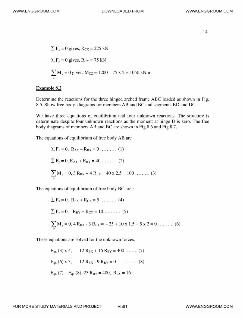
Shearing deformations
The deformations dδy and dδz due to shearing forces consist of displacement dδ of one
side of element with respect to other with respect to y and z directions.
WWW.ENGGROOM.COM DOWNLOADED FROM WWW.ENGGROOM.COM
FOR MORE STUDY MATERIALS AND PROJECT VISIT WWW.ENGGROOM.COM

-39-
dδy = GA
dxF2x μy
dδz = GA
dxF3x μz
F2x = Shear force in y-direction at coordinate x
F3x = Shear force in z-direction at coordinate x
G = Shear modulus
GA = Shear rigidity
μy, μz = nondimensional factors depending solely upon the shape and size of cross-
section which accounts for the nonuniform distribution of shearing stresses. For
rectangular section μ = 1.2 and for circular section μ = 1.11. For I or H sections μA
can be
taken as web area or in other words μ can be taken as ratio of area of cross-section to web
area ⎟⎟⎠
⎞⎜⎜⎝
⎛=
wA
A μ .
Torsional deformation
It is given by angle of twist dθx in radians, which represents the difference in the angles
of rotation of its faces about longitudinal axis of the element.
dθx = x
4x
GI
dxF
Ix = Torsion constant or polar moment of inertia of cross section (Ix = Iy + Iz).
GIx = Torsional rigidity
F4x = Torsion moment (Mx).
WWW.ENGGROOM.COM DOWNLOADED FROM WWW.ENGGROOM.COM
FOR MORE STUDY MATERIALS AND PROJECT VISIT WWW.ENGGROOM.COM

-40-
12.2. Elastic energy of deformation
The elastic or potential energy of member of length L is given by following expression:
dx2EI
F
2EI
F
2GI
F
2GA
F
2GA
F
2EA
FU
L
oz
2
6x
y
2
5x
x
2
4x
2
3x
2
2xy 2
1xr ∫ ⎟⎟⎠
⎞⎜⎜⎝
⎛+++++= zμμ
Fex (e = 1,…,6) = components of vector of internal stress-resultants {Fx} at an arbitrary
section of member at a coordinate distance x from reference end.
rU = Elastic strain or potential energy of member number r.
U = ∑r
rU = Elastic strain or potential energy of all members of structure.
The energy due to shear is neglected being very small compared to that due to other
actions.
dx2EI
F
2EI
F
2GI
F
2EA
FU
L
oz
2
6x
y
2
5x
x
2
4x
2
1xr ∫ ⎟⎟⎠
⎞⎜⎜⎝
⎛+++=
In plane frames subjected to inplane loading primary action is bending moment only
hence energy due to axial force is neglected.
Considering only the relevant primary actions the elastic strain energy for various
structures is given by following expressions.
Axial force structures (plane and space trusses)
U = ∑r
rU = ∑r
dx2EA
FL
o
2
1x∫
Plane frames in xy-plane subjected to in plane loading
U = ∑r
rU = ∑r∫
L
oz
2
6x
2EI
dxF
WWW.ENGGROOM.COM DOWNLOADED FROM WWW.ENGGROOM.COM
FOR MORE STUDY MATERIALS AND PROJECT VISIT WWW.ENGGROOM.COM

-41-
Plane grids in xz-plane subjected to normal loading.
U = ∑r
rU = ∑r
dx2EI
F
2GI
FL
oz
2
6x
x
2
4x∫ ⎟⎟⎠
⎞⎜⎜⎝
⎛+
Space frames subjected to general loading
U = ∑r
rU = ∑r
dx2EI
F
2EI
F
2GI
F
2EA
FL
oz
2
6x
y
2
5x
x
2
4x
2
1x∫ ⎟⎟⎠
⎞⎜⎜⎝
⎛+++
There are various methods developed for computation of displacements depending upon
structural system and nature of loading but basic methods are based on energy principles
such as Castigliano’s theorem and virtual work.
12.3 Castigliano’s theorem
The partial derivative of elastic strain energy U of the structure with respect to any
external load P is equal to displacement δ in the structure corresponding to that force. The
terms force and displacement are used in the generalized sense that is word force may
mean force or moment and word displacement may mean linear or angular displacement.
Strain energy U is function of P.
P
U ∂∂
=δ
If the deflection is required at a point where there is no load, a load P is placed there and
in the expression for partial derivative of elastic energy P is set equal to zero. If the
deflection is required in the direction of a particular defined load the load is replaced with
P and finally P is set equal to prescribed value.
The deflection calculations are some what simplified if the partial derivatives are worked
out before integration.
( ) ( ) ( ) ( )∑
∫∫∫∫
⎥⎥⎥
⎦
⎤
⎢⎢⎢
⎣
⎡ ∂∂+
∂∂+
∂∂+
∂∂=
∂∂
=r z
L
6x6x
y
L
5x5x
x
L
4x4x
L
1x1x
dxEI
P/FF
dxEI
P/FF
dxGI
P/FF
EA
dxP/FF
P
U δ
WWW.ENGGROOM.COM DOWNLOADED FROM WWW.ENGGROOM.COM
FOR MORE STUDY MATERIALS AND PROJECT VISIT WWW.ENGGROOM.COM

-42-
The derivatives represent the rate of change of forces Fex with respect to P.
P
Ff,
P
Ff,
P
Ff,
P
Ff 6x
6x5x
5x4x
x41x
1x ∂∂
=∂∂
=∂∂
=∂∂
=
These derivatives f are equal to values Fex as caused by a unit load (P=1) and are
represented by fex.
∑∫∫∫∫
⎥⎥⎥
⎦
⎤
⎢⎢⎢
⎣
⎡
+++=r z
L
6x6x
y
L
5x5x
x
L
4x4x
L
1x1x
dxEI
fF
dxEI
fF
dxGI
fF
dxEA
fF
δ
12.4. Dummy load method
The equations of dummy load method are derived from principle of virtual work, hence,
it is also called virtual work method. It is also called Maxwell-Mohr method.
In this method two systems of loading of same structure are considered.
System 1: Given structure, loading, temperature variations and misfits of parts
System 2: Same structure subjected to unit action corresponding to desired displacement.
This action can be unit point load or unit moment or unit pair of opposite
forces or moments.
The opposing pair of dummy unit loads is deployed to obtain relative displacement or
rotation of two points on the structure.
According to principle of virtual work if the second system is given a small displacement
the total work of the forces will be zero.
At a point represented by local coordinate x in a member the internal stress resultants will
be fex (e = 1,….,6) due to dummy unit action. The virtual displacements of the second
system are taken as the actual displacements of the first system. Then in accordance with
the principle of virtual work.
∑ ∫∫∫∫⎥⎥⎦
⎤
⎢⎢⎣
⎡+++=
r L z
6x6x
L y
5x5x
L x
4x4x
L
1x1x dxEI
fFdx
EI
fFdx
GI
fFdx
EA
fF x1 δ
WWW.ENGGROOM.COM DOWNLOADED FROM WWW.ENGGROOM.COM
FOR MORE STUDY MATERIALS AND PROJECT VISIT WWW.ENGGROOM.COM
-43-
It will be observed that the deflection calculations using Castigliano’s theorem are the
same as in dummy load method.
12.5. Numerical examples
Example
Determine the horizontal and vertical deflections and the angle of rotation at free end A
of cantilever bracket shown in figure 12.8 neglecting axial and shear deformations. The
members AB and BC have flexural rigidity EI and axial rigidity EA. Determine
additional deflection at A if axial deformations are considered.
The structural system comprises of two members. The members are numbered 1 and 2.
The local axes xyz of members are shown. The common axes system for whole structure
is XYZ. The bending moment diagrams due to given loading, unit horizontal and vertical
and unit couple at A are shown in Fig.12.9. The displacements are computed in system
coordinates XYZ.
Vertical deflection at A
dxEI
fF-
r L
6x6xY ∑∫=δ
r = 1: 3EI
Pa dx
EI
Px x 3a
o=∫
r = 2: EI
hPa dx
EI
a Pa 2h
o=∫
⎥⎦
⎤⎢⎣
⎡+=
3EI
Pa
EI
hPa-
32
Yδ
Horizontal deflection at A
dxEI
fF
r
6x6xX ∑+=δ
WWW.ENGGROOM.COM DOWNLOADED FROM WWW.ENGGROOM.COM
FOR MORE STUDY MATERIALS AND PROJECT VISIT WWW.ENGGROOM.COM

WWW.ENGGROOM.COM DOWNLOADED FROM WWW.ENGGROOM.COM
FOR MORE STUDY MATERIALS AND PROJECT VISIT WWW.ENGGROOM.COM

-44-
r = 1: 0 dx EI
0Px x a
o=∫
r = 2: ( )
2EI
Pah
2EI
Pah
EI
h Pa dx
EI
x-hPa 222h
o=−=∫
2EI
Pah
2
X =δ
Rotation at A
dxEI
fF
r
6x6xZ ∑−=θ
r = 1: 2EI
Pa dx
EI
1Px x 2a
o=∫
r = 2: EI
Pah dx
EI
1 x Pah
o=∫
⎥⎦
⎤⎢⎣
⎡+−=
EI
Pah
2EI
Pa2
Zθ
Effect of axial forces
dxEA
fF-
r
1x1xY ∑=δ
r = 2: EA
Ph dx
EA
1 x Ph
o=∫
EA
ph - Y =δ
WWW.ENGGROOM.COM DOWNLOADED FROM WWW.ENGGROOM.COM
FOR MORE STUDY MATERIALS AND PROJECT VISIT WWW.ENGGROOM.COM

-45-
Example
Determine horizontal and vertical displacement of point C and horizontal movement of
roller of plane truss shown in figure 12.10.
A1 = A2 = 150 mm2, A3 = 100 mm
2, E = 200 kN/mm
2
L1 = L2 = 5000 mm, L3 = 8000 mm.
Computation for given loading
RA = RB = 3 kN
Sin θ 5
3 = , cos θ
5
4 =
F1 sin θ = 3, F1 3
5 x 3 = = 5 kN (C)
F2 sin θ = 3, F2 3
5 x 3 = = 5 kN (C)
F3 = F2 cos θ = 5 x 5
4 = 4 kN (T)
Unit load at C in y-direction
F1 sin θ = 2
1 , F1 =
6
5 (T)
F2 sin θ = 1, F2 = 6
5 (T)
F3 = F1 cos θ = 6
5 x
5
4 =
3
2 (C)
WWW.ENGGROOM.COM DOWNLOADED FROM WWW.ENGGROOM.COM
FOR MORE STUDY MATERIALS AND PROJECT VISIT WWW.ENGGROOM.COM

WWW.ENGGROOM.COM DOWNLOADED FROM WWW.ENGGROOM.COM
FOR MORE STUDY MATERIALS AND PROJECT VISIT WWW.ENGGROOM.COM

-46-
Unit load at C in x-direction
8 RB = 3 x 1, RB = ↑8
3
8 RA = 3 x 1, RA = ↓8
3
Joint A
F1 sin θ = 8
3 , F1 =
8
5 (T)
F3 = 1 - 8
5 cos θ = 1 -
2
1 =
2
1 (T)
Joint B
F2 sin θ = 8
3 , F2 =
8
5 (C)
Joint C
2 x 8
5 cos θ = 1 (check)
Unit load at B in x-direction
RAV = RBV = 0, RAH = 1 kN
F1 = F2 = 0
F3 = 1 (T)
WWW.ENGGROOM.COM DOWNLOADED FROM WWW.ENGGROOM.COM
FOR MORE STUDY MATERIALS AND PROJECT VISIT WWW.ENGGROOM.COM

-47-
F1f1
Member
L
(mm)
A
(mm2)
F1
(kN) AE
L
f1XC
(kN)
f1YC
(kN)
f1XB
(kN) XC YC XB
3(AB)
2 (BC)
1 (CA)
8000
5000
5000
100
150
150
+ 4
- 5
- 5
5
2
6
1
6
1
+ 2
1
- 8
5
+ 8
5
-3
2
+6
5
+ 6
5
+ 1
0
0
+ 2
+8
25
- 8
25
-3
8
-6
25
- 6
25
+ 4
0
0
F1 = Axial force in member due to given loads
f1XC , f1YC, f1XB = Axial force in member due to unit loads in X and Y directions at point
C and B.
δxc = ∑=
3
1r
11
AE
LfF = 2 x
5
2 +
8
25 x
6
1 -
8
25 x
6
1 =
5
4 = 0.8 mm
δyc = ∑=
3
1r
11
AE
LfF = -
3
8 x
5
2 -
6
25 x
6
1 -
6
25 x
6
1 = 2.46 mm
δXB = ∑=
3
1r
11
AE
LfF = 4 x
5
2 = o.8 mm
Check
Horizontal movement of roller is equal to extension of bar 3.
(ΔL)3 = 3AE
FL⎟⎠⎞
⎜⎝⎛
= 200 x 100
8000 x 4 1.6 mm.
(ΔL)3 = δxc + δXB = 0.8 + 0.8 = 1.6 mm.
Example
Determine displacement in the direction of load P acting at A of a cantilever bracket as
shown in figure 12.11.
WWW.ENGGROOM.COM DOWNLOADED FROM WWW.ENGGROOM.COM
FOR MORE STUDY MATERIALS AND PROJECT VISIT WWW.ENGGROOM.COM

WWW.ENGGROOM.COM DOWNLOADED FROM WWW.ENGGROOM.COM
FOR MORE STUDY MATERIALS AND PROJECT VISIT WWW.ENGGROOM.COM

-48-
Following numerical data is given. Bars are circular in section.
a = 100 mm, h = 200 mm, φ = 100 mm, E = 200 kN/mm2, G = 70 kN/mm
2, P = 200 kN
The two members are separated as shown in Fig.12.12. Their local axes x1, y1, z1 and x2,
y2, z2 are shown. The free bodies of the two members are prepared and BM and TM
diagrams are shown for P and P = 1.
δ = ∑∫∫
= ⎥⎥⎥
⎦
⎤
⎢⎢⎢
⎣
⎡
+2
1r y
L
5x5x
x
L
4x4x
dxEI
fF
dx GI
fF
For circular section
Ix = Iy + Iz
Iy = Iz = 644
10 x 909.464
100 x
64==
ππφmm
4, Ix = 9.818 x 10
6 mm
4
Member no I
The member is subjected to primary action of bending moment about y1-axis.
δA1 = Deflection of A due to deformation of member 1 that is deflection of A with respect
to B if B is clamped.
δA1 = 6
3
y
3a
o y
2
10 x 4.909 x 200 x 3
100x200
3EI
Pa dx
EI
Px==∫ = 0.068 mm
Member 2
The member no.2 is subjected to primary actions of bending moment about y2-axis and
torsion moment about x2-axis.
δA2 = Deflection A due to deformation of member 2.
δA2 = x
2
y
3h
o
2
x
h
o
2
y GI
hPa
EI3
PhdxPa
GI
1 dx Px
EI
1+=+ ∫∫
WWW.ENGGROOM.COM DOWNLOADED FROM WWW.ENGGROOM.COM
FOR MORE STUDY MATERIALS AND PROJECT VISIT WWW.ENGGROOM.COM
-49-
δA2 = 6
2
6
3
10x 9.818 x 70
200x 100x200
10 x 4.909 x 200 x 3
200 x 200 + = 0.543 + 0.582
Therefore δA = 0.068 + 0.543 + 0.582 = 1.193 mm
Check
θBC = Angle of twist of B with respect C = ( )( )
GI
hPa
x
=610x 9.818x 70
200 x 100 x 200 = 5.82 x 10
-3
radians
Displacement of A due to twist = 5.82 x 10-3
x 100 = 0.582 mm.
13 NONPRISMATIC MEMBERS
A nonprismatic member has a variable section along its length. For any structural
member, the stress resultants do not remain constant throughout its length. Where there is
a significant variation of the stress resultants along the length of member, economy can
be achieved more efficiently by varying the cross-sectional area of the member, keeping
in view the extreme values of the stress resultants in the middle and end sections. Often
such variation can be adopted to add to the architectural appearance of the structure.
Generally, two types of members are used:
(1) Members with parabolic haunches or parabolic variation of depth.
(2) Members with straight haunches or with linear variation of depth.
The axis of member with haunches or with variable depth is assumed to be the same as
for the uniform part usually in the central portion of the member. For a tapered member
the uniform part will correspond to the minimum section.
Analysis of such members shown in Fig.13.1 to 13.4 involves the determination of fixed
end reactions due to self weight and loads acting on the members and the flexibility and
stiffness properties that is force-displacement relationships. For haunched members the
fixed end moments, stiffness and flexibility properties are expressed in terms of integrals
or bar constants. The bar constants are available in handbooks.
WWW.ENGGROOM.COM DOWNLOADED FROM WWW.ENGGROOM.COM
FOR MORE STUDY MATERIALS AND PROJECT VISIT WWW.ENGGROOM.COM

WWW.ENGGROOM.COM DOWNLOADED FROM WWW.ENGGROOM.COM
FOR MORE STUDY MATERIALS AND PROJECT VISIT WWW.ENGGROOM.COM

-50-
13.1 Fixed end reactions
Fixed end reactions for bending in xy-plane.
Concentrated vertical load F and udl of intensity ω will be considered as shown in Fig.
13.5.
(1) Concentrated vertical load F acting at a distance a from left end.
( )
( ) ( )
∫ ∫ ∫
∫ ∫ ∫ ∫
⎟⎟⎠
⎞⎜⎜⎝
⎛−
−=
L
o
L
o
2L
o zz
2
z
L
o
L
a
L
o
L
a zz
2
zz
Az
I
xdx
I
dxx
I
dx
I
dxa -x
I
dxx
I
dxa-xx
I
xdx
FM
(2) Uniformly distributed vertical load of intensity ω acting on whole span.
( )
∫ ∫ ∫
∫ ∫ ∫
⎟⎟⎠
⎞⎜⎜⎝
⎛−
⎟⎟⎠
⎞⎜⎜⎝
⎛−
=L
o
L
o
2L
o zz
2
z
L
o
L
o
2L
o z
2
z
3
z
Az
I
xdx
I
dxx
I
dx
I
dxx
I
dxx
I
xdx
2
Mω
The fixed end moment at the right end B can be determined by performing the
integrations in the opposite direction. The vertical reactions at the two ends can be
determined from the equilibrium of the free body of the member. The case of bending in
xz-plane is treated similarly.
Fixed end reactions for torsion moment
For concentrated torsion moment T acting at intermediate point of member at distance a
from left end as shown in Fig.13.6, the fixed end torsional moments are determined from
the condition of compatibility at the point of application of the external torsional moment.
The angle of twist θ for the two parts namely the left and right cantilevered segments is
the same. The left segment is shown in Fig. 13.7 and 13.8. The haunch is shown in
Fig.13.9.
The angle of twist between any section on the uniform part of the haunched beam and the
fixed end is given by:
WWW.ENGGROOM.COM DOWNLOADED FROM WWW.ENGGROOM.COM
FOR MORE STUDY MATERIALS AND PROJECT VISIT WWW.ENGGROOM.COM

WWW.ENGGROOM.COM DOWNLOADED FROM WWW.ENGGROOM.COM
FOR MORE STUDY MATERIALS AND PROJECT VISIT WWW.ENGGROOM.COM

WWW.ENGGROOM.COM DOWNLOADED FROM WWW.ENGGROOM.COM
FOR MORE STUDY MATERIALS AND PROJECT VISIT WWW.ENGGROOM.COM

-51-
θ = ⎟⎟⎠
⎞⎜⎜⎝
⎛+
U
U
H
H
J
L
J
L
G
T
LH = Length of haunched part
LU = Length of uniform part
JH = Torsion constant of haunched part
JU = Torsion constant of uniform part
JH = ( )
b
dfor
b63.0d
b63.0dlog 3
ddb
1
2e
12
3
⎟⎟⎠
⎞⎜⎜⎝
⎛−−−
> 1.2
JU = b
dfor
d
b 0.63 - 1
3
db3
⎟⎠⎞
⎜⎝⎛
> 1.2
The torsional stiffness factor Kt for a member with haunched and uniform parts is given
by:
Kt =
⎟⎟⎠
⎞⎜⎜⎝
⎛+
H
H
U
U
J
L
J
L
G
The fixed end torsional moments TA and TB are expressed as:
TA = ( )
( ) ( )BtAt
At
K K
KT
+
TB = ( )
( ) ( )BtAt
Bt
K K
KT
+
The fixed end reactions for the case of uniformly distributed torque can be worked out in
similar manner.
WWW.ENGGROOM.COM DOWNLOADED FROM WWW.ENGGROOM.COM
FOR MORE STUDY MATERIALS AND PROJECT VISIT WWW.ENGGROOM.COM

-52-
Fixed end reactions for axial force
The fixed end reactions PA and PB for axial force P acting at any point on uniform part of
a haunched member as shown in Fig.13.10 are given by:
PA = ( )
( ) ( )BFAF
AF
K K
K P
+
PA = ( )
( ) ( )BFAF
BF
K K
K P
+
KF =
⎟⎟⎠
⎞⎜⎜⎝
⎛+
H
H
U
U
A
L
A
L
E
AH = ( )
d
dlog
ddb
1
2e
12 −
The equivalent uniform area Aeq of member of variable section is given in terms of area
Ax at coordinate x.
L
dxA
1
A
1
L
o x
eq
∫=
Axial rigidity = L
EAeq
The fixed end reactions for the case of uniformly distributed axial force can be worked
out in a similar manner.
Like fixed end reactions the bar constants are also expressed in terms of integrals.
Evaluation of integrals from first principles is cumbersome hence, use is made of hand
books to save this labour.
13.2 Basic concepts and definitions of bar constants of members with variable section
Ends of member of length L are designated by A and B.
WWW.ENGGROOM.COM DOWNLOADED FROM WWW.ENGGROOM.COM
FOR MORE STUDY MATERIALS AND PROJECT VISIT WWW.ENGGROOM.COM

-53-
Rotational stiffness factor
The rotational stiffness factor K at one end of member, which is assumed hinged, is
defined as the moment required to produce a unit rotation at this end, while the other end
is assumed to be fixed as shown in Fig.13.11.
In hand books the stiffness factor K at an end of a haunched member is given as:
K = L
kEImin
k = Stiffness coefficient
E = Modulus of elasticity
Imin = Minimum moment of inertia of member
L = Length of member
Carry over factor
The carry over factor C from the near end to the far end of a bar is defined as the ratio of
the moment induced at far end, which is assumed fixed, to the applied moment at the near
end which is assumed hinged. The product of the carry over factor and the rotational
stiffness factor at one end of member AB is equal to similar product at the other end.
CAB KAB = CBA KBA
Modified rotational stiffness factor
The modified rotational stiffness factor K′ at one end of the member is defined as the
moment required to produce unit rotation at this end which is assumed hinged when the
other end is also hinged as shown in Fig.13.12.
ABK′ = KAB (1 – CAB CBA)
BAK′ = KBA (1 – CBA CAB)
WWW.ENGGROOM.COM DOWNLOADED FROM WWW.ENGGROOM.COM
FOR MORE STUDY MATERIALS AND PROJECT VISIT WWW.ENGGROOM.COM

WWW.ENGGROOM.COM DOWNLOADED FROM WWW.ENGGROOM.COM
FOR MORE STUDY MATERIALS AND PROJECT VISIT WWW.ENGGROOM.COM

-54-
Lateral stiffness factor
The lateral- stiffness factor K at one end of the member, which is assumed fixed against
rotation, is defined as the moment produced at this end when the other end also fixed
against rotation, is displaced laterally through unit distance with respect to the first end,
as shown in Fig.13.13.
K AB = L
KAB (1 + CAB)
K BA = L
KBA (1 + CBA)
Modified lateral stiffness factor
The modified lateral stiffness factor ′
K at one end of a member, which is assumed fixed
against rotation is defined as the moment produced at this end when the other end,
assumed hinged, is displaced laterally through unit distance with respect to first end as
shown in Fig.13.14.
ABK′ = L
KAB (1 - CAB CBA)
BAK′ = L
KBA (1 - CBA CAB)
14 SLOPE DEFLECTION EQUATIONS
Sign convention
Clockwise moments and rotations at the end of bar are treated positive. The lateral
displacement between two ends of bar resulting in positive end moments or counter
clockwise lateral displacement angle ψ is treated as positive. The shear causing clockwise
moment in the bar is treated as positive. The external loads acting vertically downwards
are treated positive as shown in Fig.14.1.
The force displacement relationship at the nodes of the elastic bar is defined by following
slope deflection equations:
MAB = MFAB + KAB θA + CBA KBA θB + L
ΔKAB (1 + CAB)
WWW.ENGGROOM.COM DOWNLOADED FROM WWW.ENGGROOM.COM
FOR MORE STUDY MATERIALS AND PROJECT VISIT WWW.ENGGROOM.COM

-55-
MBA = MFBA + KBA θB + CAB KAB θA + L
ΔKBA (1 + CAB)
MFAB, MFBA = Fixed end moments at ends A and B.
Designating A as near end and B as far end of member, the two slope deflection
equations can be written as:
Mnear = MFnear + Knear θnear + Cfar Kfar θfar + L
ΔKnear (1 + Cnear)
For a bar of uniform section:
Cnear = Cfar = 2
1
Knear = Kfar = L
EI4
Mnear = MFnear + ⎥⎦⎤
⎢⎣⎡ Δ
++L
32
L
EI2farnear θθ
Example
Find the fixed end moments and reactions for the fixed beam AB loaded as shown in
figure 14.2 and due to downward sinking of support B of 10 mm. E = 15 kN/mm2.
From handbook of bar constants the desired coefficients are taken.
aA = 6
1.2= 0.2, rA =
400
240= 0.6
aB = 6
1.8= 0.3, rB =
400
160= 0.4
For 4 kN load
FEM coeff at A = 0.1371
FEM coeff at B = 0.0327
WWW.ENGGROOM.COM DOWNLOADED FROM WWW.ENGGROOM.COM
FOR MORE STUDY MATERIALS AND PROJECT VISIT WWW.ENGGROOM.COM

-56-
For 3 kN load
FEM coeff at A = 0.0642
FEM coeff at B = 0.1754
MFAB = ∑ (FEM Coeff)A WL
MFAB = 0.137 x 4 x 6 + 0.0642 x 3 x 6 = 4.446 kNm
MFBA = ∑ (FEM Coeff)B WL
= 0.0327 x 4 x 6 + 0.1754 x 3 x 6 = 3.942 kNm
Fixed end moments due to lateral displacement of B with respect to A.
From handbook of bar constants:
kAB = 6.48, kBA = 6.68, CAB = 0.622, CBA = 0.604
Δ = 10 mm, L = 6000 mm, Imin = 12
400 x 250 3
= 1333.333 x 106 mm
4
KAB = 6000
15x 10 x 1333.333 x 6.48
L
EIk 6
minAB = = 216 x 105 kN mm
MFAB = L
ΔKAB (1 + CAB) =
6000
10x 216 x 10
5 (1.622) = 58,392 kN mm
KBA = 6000
10 x 1333.333 x 15 x 6.68
L
EIk 6
minBA = = 222 x 105 kN mm
MFBA = L
Δ KBA (1 + CBA) =
6000
10x 222 x 10
5 x 1.604 = 59348 kN mm
Total fixed end moments due to loads and relative displacement of supports:
MAB = 4.446 + 58.392 = 62.838 kN m
MBA = 3.942 + 59.348 = 55.406 kN m
WWW.ENGGROOM.COM DOWNLOADED FROM WWW.ENGGROOM.COM
FOR MORE STUDY MATERIALS AND PROJECT VISIT WWW.ENGGROOM.COM

-57-
Reactions are computed from free body shown in Fig.14.3.
6RA = 62.838 – 55.406 + 3 x 1.8 + 4 x 4.8
RA = 5.339 kN
6RB = - 62.838 + 55.403 + 4 x 1.2 + 3 x 4.2
RB = 1.661 kN
RA + RB = 7 kN (check)
Example
A 4 m span fixed tapered beam AB of section 250 x 560 mm at A and 250 x 280 mm at B
is subjected to udl of intensity 5 kN/m as shown in Fig.14.4. Using hand book of bar
constants determine fixed end moments and hence reactions.
aA = 1.0, aB = 0, rA = 560
280= 0.5, rB = 0
Fixed end moment coeff at A = 0.1216
Fixed end moment coeff at B = 0.0529
FEM = coeff x w x L2
MFAB = 0.1216 x 5 x 4 x 4 = 9.728 kN m
MFBA = 0.0529 x 5 x 4 x 4 = 4.232 kN m
The reactions are computed from free body shown in Fig.14.5.
RA = 4
1[9.728 + 5 x 4 x 2 – 4.232] = 11.374 kN
RB = 4
1[4.232 + 5 x 4 x 2 – 9.728] = 8.626 kN
RA + RB = 11.374 + 8.626 = 20 kN (check)
WWW.ENGGROOM.COM DOWNLOADED FROM WWW.ENGGROOM.COM
FOR MORE STUDY MATERIALS AND PROJECT VISIT WWW.ENGGROOM.COM

-58-
15 MOMENT DISTRIBUTION METHOD
The slope deflection method involves solution of many simultaneous equations. The
moment distribution method does not involve as many simultaneous equations. The
number of equations reduces considerately and in case of structures with no lateral
displacements of nodes of members there are no equations to be solved. Hence, the
computational work is much less in this method compared to other methods. This method
has an additional advantage as it is based on iterative technique consisting of series of
cycles of clamping and unclamping of the joints of structure, each cycle converging on
the precise final result. Therefore, the series of cycles can be terminated when the desired
degree of accuracy of results has been achieved.
The moment at each end of a member as can be seen from slope-deflection equations
comprises of four separate effects.
(1) Fixed end moment (FEM) at the end under consideration due to applied load on the
member.
(2) Rotation of member at near end.
(3) Rotation of member at far end.
(4) Rotation of axis or chord of member or the lateral displacement of nodes.
In moment distribution method these effects are considered separately and results are
superimposed. Consider a joint A where four members meet rigidly as shown in figure
15.1. The far ends of members are clamped. An artificial clamp is introduced at A. The
structure is now kinematically determinate comprising of fixed ended members and the
fixed end moments can be computed for the external loads applied to members. The
degree of freedom of this structure is one that is rotation at A. Since far ends are clamps
they neither rotate nor displace laterally.
If the algebraic sum of fixed end moments at A does not vanish, the resultant moment
acting at the joint is termed unbalanced moment. The artificial clamp holds or balances
this unbalanced moment.
If now the artificial clamp is removed the joint will rotate under the action of unbalanced
moment as shown in Fig.15.2 and end moments will develop in all the members as shown
in Fig.15.3. The moments developed at A due to rotation restore the equilibrium of joint
and are called distributed moments. The moments developed at far ends are called carry-
over-moments. Same sign convention is followed as in slope deflection method.
M = Unbalanced moment at A = ( )∑A
FEM
WWW.ENGGROOM.COM DOWNLOADED FROM WWW.ENGGROOM.COM
FOR MORE STUDY MATERIALS AND PROJECT VISIT WWW.ENGGROOM.COM
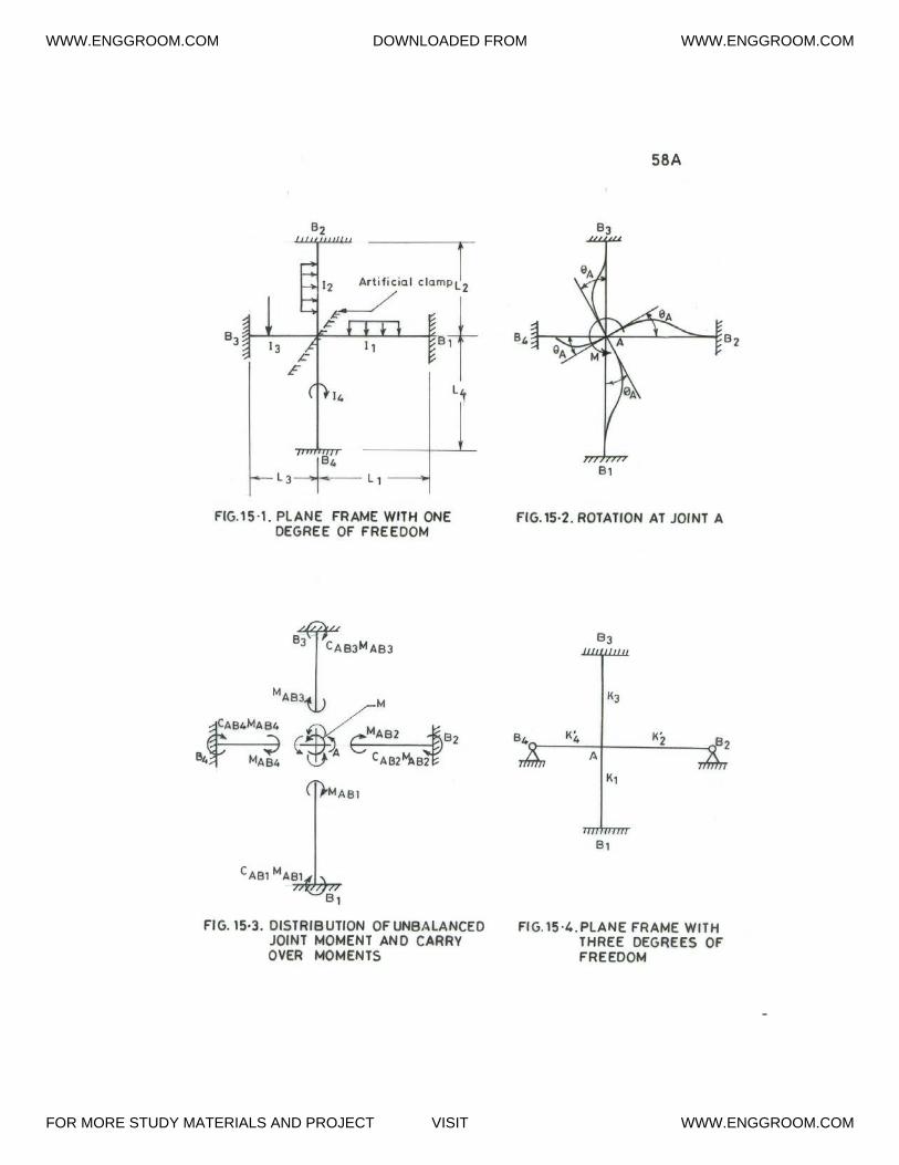
-
WWW.ENGGROOM.COM DOWNLOADED FROM WWW.ENGGROOM.COM
FOR MORE STUDY MATERIALS AND PROJECT VISIT WWW.ENGGROOM.COM
-59-
When clamp at A is removed or relaxed as it is called the structure deforms further and
develops distributed member end moments at A and carry over moments at B1 to B4.
For moment joint equilibrium at A:∑A
M = 0
M + MAB1 + MAB2 + MAB3 + MAB4 = 0
θB1 = θB2 = θB3 = θB4 = 0
MAB1 = KAB1 θA
MAB2 = KAB2 θA
MAB3 = KAB3 θA
MAB4 = KAB4 θA
θA ⎥⎦
⎤⎢⎣
⎡∑A
ABK + M = 0
θA = ∑
A
ABK
M -
MAB1 = ∑
A
AB
AB1
K
K -M = - (DF)AB1 M
Similarly expression for moments at end A for other members can also be written.
(DF)AB1 = Distribution factor at joint A for member AB1.
(DF)AB1 = ∑
A
AB
AB1
K
K
The distributed moment developed at the relaxed end of member under unbalanced
moment M at corresponding joint is equal to distribution factor (DF) of this member at
this joint times the unbalanced moment with the sign reversed.
The carry over moment at end B1 will be: MB1A = CAB1 MAB1
WWW.ENGGROOM.COM DOWNLOADED FROM WWW.ENGGROOM.COM
FOR MORE STUDY MATERIALS AND PROJECT VISIT WWW.ENGGROOM.COM

-60-
The carry-over moment to far end is equal to carry over factor times the corresponding
distributed moment and has the same sign.
If far end of a member is hinged then modified stiffness of the member is to be taken in
computation of distribution factors as shown in figure 15.4. B1 and B3 are clamps and B2
and B4 are hinges.
4321
A
AB KKKKK ′++′+=∑
(DF)AB2 = ∑
′
A
AB
AB2
K
K
Cantilever portions of structure
The cantilever portions of the structure can be taken care of in two ways
(1) The effect of loads acting on cantilever can be transferred to nearest joint and
cantilever part removed as shown in figure 15.5. Nearest joint will be subjected to
externally applied vertical load and a moment. This moment is to be taken at this joint
as external moment. For the case under consideration the vertical load will be (P+Q)
and moment will be (PL+Qa) as shown in figure 15.5. Now the continuous beam
ABCD can be analyzed by moment distribution method. D is now a simple support.
Distribution factor for DC will be 1. There will be no carry over from C to D. For CD
modified stiffness is used for the moment distribution process.
(2) The continuous beam ABCDE is retained as it is and the cantilever part DE is not
knocked out. Cantilever moment is entered as FEM for DE. The DF at D will be 1 for
DC and zero for DE. Since member is now continuous over support D there will be
carry over of moments from C to D and rotational stiffness of CD will not be
modified in view of fact that D is not an end simple support as for case when
cantilever is knocked out. The moments DE and DC will be of same magnitude and
equal to cantilever moment but of opposite sign.
It may be noted that cantilever arm has no restraining effect on the rotation of joint to
which it is rigidly connected or in other words its stiffness is zero. Any unbalanced
moment is therefore carried or distributed entirely by other members meeting at this joint.
In the moment distribution process all the hinged joints should be released first for quick
convergence. As regards other joints one should start with the joint which has largest
unbalanced moment for rapid convergence. The final results are not affected by the order
of relaxation of joints.
WWW.ENGGROOM.COM DOWNLOADED FROM WWW.ENGGROOM.COM
FOR MORE STUDY MATERIALS AND PROJECT VISIT WWW.ENGGROOM.COM

WWW.ENGGROOM.COM DOWNLOADED FROM WWW.ENGGROOM.COM
FOR MORE STUDY MATERIALS AND PROJECT VISIT WWW.ENGGROOM.COM

-61-
In the structures where only rotation of joints is involved no simultaneous equations are
required to be solved. Such structures have no side sway. For structures undergoing side
sway the number of equations to be framed and solved will be equal to number of
unknown lateral displacements Δ or the side sway angles or chord angles ψ.
For problems involving side sway the solution by moment distribution is carried out in
two separate parts.
(1) Moment distribution analysis for no sway.
For this artificial constraints are introduced in structure so that there is no sway and
reactions are determined at these constraints.
(2) Moment distribution analysis for lateral sway.
Now the structure is subjected to lateral displacements Δ1, Δ2, … , Δn or ψ angles
ψ1,ψ2, …, ψn corresponding to n constraints introduced and moment distribution
analysis is carried out and reactions computed at the n constraints in terms of Δ1, Δ2,
… , Δn. Thus frame is to be analyzed for (n + 1) number of cases. After adding the
results of sway and non-sway moment distribution cases, the reactions at the
constraints are set equal to zero as they do not exist. Therefore n is corresponding to
degree of freedom of structure corresponding to lateral displacements. After lateral
displacements are computed, the moments and other desired data can be obtained.
Methodology
The methodology is explained on single bay two storey frame as shown in figure 15.6.
Degree of freedom with respect to side sway = 2.
Δ2 = Side sway at level CF with respect to level at BE.
Δ1 = Side sway at level BE.
There will be two independent ψ-angles ψ1 and ψ2 corresponding to lateral displacements
Δ1 and Δ2.
This frame will have to be analyzed for (n+1) = (2+1) = 3 cases. The side sway is
prevented by introducing two constraints as shown in figure 15.7 and the frame is
analyzed by moment distribution for no sway case and reactions R1 and R2 determined at
the fictitious constraints. Now constraint at E is given unit displacement to right without
imparting any rotations to joints B, E, C and F as shown in Fig.15.8. The frame is
analyzed and reactions R1A and R2A are determined. Now constraint at F is given unit
WWW.ENGGROOM.COM DOWNLOADED FROM WWW.ENGGROOM.COM
FOR MORE STUDY MATERIALS AND PROJECT VISIT WWW.ENGGROOM.COM

-62-
lateral displacement without rotations at joints B, E, C and F as shown in Fig.15.9. The
frame is analyzed and reactions R1B and R2B are determined. Since artificial constraints
are introduced the total reaction at the two constraints for combined three cases should
vanish.
R1 + R1A Δ1 + R1B Δ2 = 0
R2 + R2A Δ1 + R2B Δ2 = 0
H,
H,
H
1
2
22
1
11
Δ=Ψ
Δ=Ψ
Δ=Ψ
The two equations are solved for Δ1 and Δ2 and moments obtained in the two sway cases
are modified by substituting the values of Δ1 and Δ2 respectively. Now sway and non
sway moments are added to get final result.
It may be mentioned here that Kani’s method which is also based on iteration technique
does not involve solution of any simultaneous equations. Kani’s method will not be
discussed here.
The method of moment distribution will be demonstrated by solving same problems as in
case of slope deflection method as shown in figure 15.10.
Example 15.1.
This problem will be solved in two stages.
Stage 1 : For vertical loads
Stage 2 : For concentrated moment at joint B
KBA = 22,200 kNm, KBC = 33,350 kNm
∑B
K = KBA + KBC = 55,550 kNm
(DF)BA = 550,55
200,22 = 0.4, (DF)BC =
550,55
350,33 = 0.6
CBA = 0.604, CBC = 0.294
WWW.ENGGROOM.COM DOWNLOADED FROM WWW.ENGGROOM.COM
FOR MORE STUDY MATERIALS AND PROJECT VISIT WWW.ENGGROOM.COM

WWW.ENGGROOM.COM DOWNLOADED FROM WWW.ENGGROOM.COM
FOR MORE STUDY MATERIALS AND PROJECT VISIT WWW.ENGGROOM.COM

-63-
MFAB = - 44.46 kNm, MFBA = + 39.45 kNm
MFBC = - 9.37 kNm, MFCB = + 4.23 kNm
The moment distribution for concentrated moment at joint B is carried out separately. It
is entered on top of the joint and then distributed. The moments at the ends of members
for the two cases are now added to obtain final moments.
The reactions can be computed from free body diagrams of supports shown in Fig.15.11.
Moment distribution for vertical loads.
JOINT A B B C
DF & COF 0.604 ← 0.4 0.6 → 0.294
FEM
DC
COC
-44.46 + 39.45
- 12.03
- 7.27
- 9.37 + 4.23
- 18.05
- 5.31
TOTAL - 51.73 + 27.42 - 27.42 - 1.08
Moment distribution for concentrated moment.
-5
JOINT A B B C
DF & COF 0.604 ← 0.4 0.6 → 0.294
DC
COC
- 2.00
+ 1.21
+ 3.00
+ 0.88
TOTAL + 1.21 + 2.00 + 3.00 + 0.88
WWW.ENGGROOM.COM DOWNLOADED FROM WWW.ENGGROOM.COM
FOR MORE STUDY MATERIALS AND PROJECT VISIT WWW.ENGGROOM.COM

-64-
Final moments
-5
JOINT A B B C
DF & COF 0.604 ← 0.4 0.6 → 0.294
CASE1
CASE2
- 51.73 + 27.42
+ 1.21 + 2.00
- 27.42 - 1.08
+ 3.00 + 0.88
TOTAL - 50.52 + 29.42 - 24.42 - 0.20
Beam AB
RA = ( )
6
42.2952.50
6
1.8x 30
6
4.8x 40 −++ = 32 + 9 + 3.52 = 44.52 kN
RBA = 6
52.5042.29
6
4.2x 30
6
1.2x 40 −++ = 8 + 21 – 3.52 = 25.48 kN
RA + RBA = 44.52 + 25.48 = 70 kN (ok)
Beam BC
RBC = 4
0.2 42.24 ++ 5 x 2 = 6.12 + 10 = 16.12 kN
RC = 5 x 2 - 4
0.2 42.24 += 10 – 6.12 = 3.88 kN
RBC + RC = 16.12 + 3.88 = 20 kN (ok)
Total reaction at support B:
RB = RBA + RBC = 25.48 + 16.12 = 41.6 kN
Example 15.2
The portal frame with unequal legs loaded as shown figure 15.12 is analyzed by moment
distribution method.
WWW.ENGGROOM.COM DOWNLOADED FROM WWW.ENGGROOM.COM
FOR MORE STUDY MATERIALS AND PROJECT VISIT WWW.ENGGROOM.COM

-65-
Solution for no sway
A roller constraint is introduced at B so that lateral movement is not permitted as shown
in Figure 15.13.
R1 = Reaction developed at B acting to right.
The dotted line indicates bottom side of members.
MFAB = MFBA = 0
MFBC = - 20 kNm, MFCB = + 20 kNm
MFCD = - 30 kNm, MFDC = + 30 kNm
Distribution factors at A and C
KBC = ( )4
2I E4= 2EI, KBA =
( )3
I E3= EI
∑B
K = 3 EI
(DF)BA = 3
1, (DF)BC =
3
2
KCB = 2 EI, KCD = 3
EI2
6
EI4=
∑C
K = 2 EI + 3
8
3
EI2= EI
(DF)CB = 2 x 4
3
8
3= , (DF)CD =
4
1
8
3x
3
2=
CBA = 0, CBC = CCB = CCD = 0.5
Fixed-end-moments, distribution factors and carry over factors are entered as shown and
the distribution and carry over cycles of moment distribution method are carried out. The
final moments for no sway case are obtained.
WWW.ENGGROOM.COM DOWNLOADED FROM WWW.ENGGROOM.COM
FOR MORE STUDY MATERIALS AND PROJECT VISIT WWW.ENGGROOM.COM

-66-
MOMENT DISTRIBUTION FOR NONSWAY CASE
JOINT A B B C C D
DF & COF 0 ← 31 3
2 →0.5 0.5 ← 43
41 →0.5
FEM
DC
COC
DC
COC
DC
COC
DC
COC
DC
COC
DC
COC
DC
0.00 0.00
--- +6.67
0.00 ---
--- - 1.25
0.00 ---
--- +0.83
0.00 ---
0.00 - 0.16
0.00 ---
--- +0.11
0.00 ---
--- - 0.02
--- ---
--- + 0.01
-20.00 +20.00
+13.33 + 7.50
+ 3.75 + 6.67
- 2.50 - 5.00
- 2.50 - 1.25
+ 1.67 + 0.94
+ 0.47 + 0.84
- 0.31 - 0.63
- 0.32 - 0.16
+ 0.21 + 0.12
+ 0.06 + 0.11
- 0.04 - 0.08
- 0.04 - 0.02
+ 0.03 + 0.01
- 30.00 + 30.00
+ 2.50 ---
--- + 1.25
- 1.67 ---
--- - 0.84
+ 0.31 ---
--- + 0.16
- 0.21 ---
--- - 0.11
+ 0.04 ---
--- + 0.02
- 0.03 ---
--- - 0.02
+ 0.01 ---
Final
moments
0.00 + 6.19
- 6.19 + 29.05
- 29.05 + 30.46
Horizontal shears are computed from free body diagrams of columns shown in Figure
15.14.
RAH = 3
6.19= 2.063 kN
RCH = 10 x 3 + 10
29.05 - 30.46= 30 + 0.23 = 30.23 kN
R1 = 60 – 2.063 – 30.235 = 27.702 kN
WWW.ENGGROOM.COM DOWNLOADED FROM WWW.ENGGROOM.COM
FOR MORE STUDY MATERIALS AND PROJECT VISIT WWW.ENGGROOM.COM

WWW.ENGGROOM.COM DOWNLOADED FROM WWW.ENGGROOM.COM
FOR MORE STUDY MATERIALS AND PROJECT VISIT WWW.ENGGROOM.COM

-67-
Solution for sway
A unit lateral displacement is imparted at level BC of the kinematically determinate
system to the left without any rotations as shown in Figure 15.15.
MFAB = MFBA = 3
2
3x 3
6EI= EI
MFCD = MFDC = 6
EI
6x 6
6EI=
Multiply these FEMs by 60/EI
MFAB = MFBA = 3
2 EI x
EI
60 = 40 kNm
MFCD = MFDC = 6
EI x
EI
60 = 10 kNm
9
6EIΔ = 40, Δ = 60/EI
36
6EIΔ = 10, Δ = 60/EI
These proportional FEMs are corresponding to Δ = EI
06.
These FEMs are entered for process of moment distribution which is carried out and final
proportional moments obtained as shown in scheme of moment distribution.
WWW.ENGGROOM.COM DOWNLOADED FROM WWW.ENGGROOM.COM
FOR MORE STUDY MATERIALS AND PROJECT VISIT WWW.ENGGROOM.COM

-68-
MOMENT DISTRIBUTION FOR SWAY CASE
JOINT A B
B C C D
DF
3
1
3
2
4
3
4
1
COF 0.5←
→0.5 0.5← →0.5
FEM
Release A
COC
+ 40 + 40
- 40 --
--- - 20
--- ---
--- ---
--- ---
+ 10 + 10
--- ---
--- ---
FEM
DC
COC
DC
COC
DC
COC
DC
COC
DC
COC
DC
0 + 20
--- - 6.67
0 ---
--- +1.25
0 ---
--- - 0.83
0 ---
--- + 0.16
0 ---
--- - 0.11
0 ---
0 +0.02
--- ---
- 13.33 - 7.5
- 3.75 - 6.67
+ 2.50 + 5.00
+2.50 + 1.25
- 1.67 - 0.94
- 0.47 - 0.84
+0.31 +0.63
+0.32 +0.16
- 0.21 -0.12
- 0.06 -0.11
+0.04 +0.08
+ 10 + 10
- 2.5 ---
--- - 1.25
+1.67 ---
--- + 0.84
- 0.31 ---
--- - 0.16
+0.21 ---
--- +0.11
- 0.04 ---
--- - 0.02
+0.03
Final
Moments
0 +13.82 - 13.82 - 9.06 + 9.06 + 9.52
From the free body diagrams of columns shown in Figure 15.16 the horizontal shears are
obtained.
3
13.82R AH = = 4.61 kN,
( )6
9.52 9.06R DH
+= = 3.10 kN
WWW.ENGGROOM.COM DOWNLOADED FROM WWW.ENGGROOM.COM
FOR MORE STUDY MATERIALS AND PROJECT VISIT WWW.ENGGROOM.COM
-69-
R = Reaction at roller constraint for sway case.
R = - (4.61 + 3.10) = - 7.71 kN
MF = Modification factor
R + MF x R = 0
MF = 71.7
702.27
R
R -
−−
= = 3.593
The proportional moments for sway case are corrected by multiplying with modification
factor and added to moments obtained for nonsway case to obtain final moments for the
given problem.
MAB = 0
MBA = + 6.19 + 13.82 x 3.593 = 55.85 kNm
MBC = - 6.19 – 13.82 x 3.593 = - 55.85 kNm
MCB = + 29.05 – 9.06 x 3.593 = - 3.50 kNm
MCD = - 29.05 + 9.06 x 3.593 = + 3.50 kNm
MDC = + 30.46 + 9.52 x 3.593 = + 64.67 kNm
The results are same as obtained by slope deflection method.
16 ANALYSIS OF CONTINNOUS BEAMS AND PLANE FRAMES CONSISTING
OF PRISMATIC AND NON-PRISMATIC MEMBERS.
The continuous beams and plane frames are indeterminate structures. The following two
methods will be discussed here for analysis of such structures.
(1) Slope deflection method
(2) Moment distribution method
WWW.ENGGROOM.COM DOWNLOADED FROM WWW.ENGGROOM.COM
FOR MORE STUDY MATERIALS AND PROJECT VISIT WWW.ENGGROOM.COM

-70-
In these methods the effect of axial deformations is neglected. These are in fact
displacement methods. The unknown displacements involved are rotations and lateral
displacements at the joints. The joints of the structure are assumed to be rigid, hence, the
member end displacements for all the members meeting at the joint are the same. This is
known as the condition of compatibility. Besides compatibility, the moment equilibrium
of the joints and the lateral shear equilibrium of the storeys of frame should be satisfied.
In slope-deflection equations, the member end moments are expressed in terms of
member end rotations and relative lateral displacement and loads acting on member.
Therefore it is possible to express joint and storey equilibrium equations in terms of
unknown displacements of structure by using slope-deflection equations of all members.
This gives the system of linear algebraic equations, which is solved by conventional
methods in case of slope-deflection method and by an iterative physical relaxation
technique in case of moment distribution method. Final results are obtained in the form of
member end forces.
Slope-deflection method
The slope-deflection equation for a non-prismatic member AB is as given below. In this
equation A and B represent near and far ends.
Mnear = MFnear + Knear θnear + Cfar Kfar θfar + ( )nearnear C1KL
+Δ
For prismatic member:
Knear = Kfar = L
4EI
Cnear = Cfar = 2
1
The slope deflection equation for uniform member takes the following form.
Mnear = MFnear + ⎥⎦⎤
⎢⎣⎡ Δ
++L
32
L
2EIfarnear θθ
Mnear = MFnear + L
2EI[2θnear + θfar + 3ψ]
or Mnear = MFnear + L
4EIθnear +
L
2EIθfar +
2L
6EIΔ
WWW.ENGGROOM.COM DOWNLOADED FROM WWW.ENGGROOM.COM
FOR MORE STUDY MATERIALS AND PROJECT VISIT WWW.ENGGROOM.COM

-71-
Mnear = MFnear + L
4EI θnear +
L
2EIθfar +
L
6EIψ
Joint equilibrium equation
The free body diagram of a rigid joint A of a plane structure is shown in figure 16.1. The
joint exerts positive clockwise moments at the ends of members meeting at this joint and
is in turn reacted by the same moments in the opposite counter clockwise directions
together with an external positive moment MextA acting on it.
An external counter clockwise moment directly acting on the joint is taken positive. The
joint moment equilibrium equation is written as follows:
∑ Mnear + Mext = 0
∑A
ABM + MextA = 0
∑A
ABM = The sum of the moments acting at end A of member AB for all the members
meeting at this joint.
Shear equilibrium equation
This pertains to the vertical columns of a particular storey in a multistory frame and is
derived from the shear equilibrium conditions of that storey. The columns are assumed
free of lateral loads directly acting on them. If there are lateral loads directly acting on the
columns, the same are replaced by statically equivalent horizontal loads and concentrated
moments acting on the nodes of frame and columns assumed free of external loads for
their function in the frame.
Inclined columns and columns of different heights can be handled by writing shear
equilibrium equation accordingly.
The free body diagram of columns of a particular storey is shown in figure 16.2. The
equation of equilibrium for a typical column AB shown in figure 16.3 is written as
follows:
MAB + MBA + HAB hAB = 0
hAB = height of column AB
WWW.ENGGROOM.COM DOWNLOADED FROM WWW.ENGGROOM.COM
FOR MORE STUDY MATERIALS AND PROJECT VISIT WWW.ENGGROOM.COM

WWW.ENGGROOM.COM DOWNLOADED FROM WWW.ENGGROOM.COM
FOR MORE STUDY MATERIALS AND PROJECT VISIT WWW.ENGGROOM.COM

WWW.ENGGROOM.COM DOWNLOADED FROM WWW.ENGGROOM.COM
FOR MORE STUDY MATERIALS AND PROJECT VISIT WWW.ENGGROOM.COM

-72-
MAB, MBA = moments at top and bottom taken positive clockwise.
HAB = shear in column taken positive acting to left at bottom.
HAB = - AB
BAAB
h
MM +
Let Qr be the external storey shear for the rth
storey of frame, which is taken positive
when acting to right. It is equal to sum of all the external horizontal loads acting on the
frame above this storey.
∑r
ABH = Reactive rth
storey shear which is sum of base shears of all the columns of this
storey.
The shear equilibrium equation for the rth
storey is:
Qr - ∑r
ABH = 0
( )∑ +
r AB
BAAB
h
MM + Qr = 0
First storey
The columns of first storey are rigidly connected to the nodes of frame at their upper
ends, their lower ends being either clamped or hinged to the foundation while the
columns of the other upper storeys are rigidly connected at both the ends. In order that
the rth
storey shear equilibrium equation is also valid for the first storey, the hinged
column need to be replaced with equivalent column fixed at base. For structural similarity
of the original hinged column and the substitute fixed column the following conditions
should be satisfied as shown in figure 16.4.
MABO = MABS
θO = θS
ΔO = ΔS
WWW.ENGGROOM.COM DOWNLOADED FROM WWW.ENGGROOM.COM
FOR MORE STUDY MATERIALS AND PROJECT VISIT WWW.ENGGROOM.COM

-73-
These conditions give:
KABS = 4
3 KABO
hABS = 2
3hABO
KABO, KABS = Rotational stiffnesses of original hinged and substitute fixed columns.
hABO, hABS = Heights of original hinged and substitute fixed columns.
The method will be demonstrated on numerical examples.
Numerical example on continuous beam
Shown in figure 16.5 is a two span continuous beam of variable section. The continuous
beam is fixed at A and C and is roller supported at B. The degree of freedom is one that is
rotation θB at B which is unknown.
θA = θC = 0
The haunched member AB and the tapered member BC were discussed in previous
sections hence the required properties are reproduced below.
Member AB Member BC
MFAB = - 44.46 kNm MFBC = - 9.37 kNm
MFBA = 39.45 kNm MFCB = 4.23 kNm
CAB = 0.622 CBC = 0.294
CBA = 0.604 CCB = 0.834
KAB = 21,600 kNm KBC = 33,350 kNm
KBA = 22,200 kNm KCB = 11,780 kNm
Slope-deflection equations:
MAB = MFAB + KAB θA + CBA KBA θB MBC = MFBC + KBC θB + CCB KCB θC
MBA = MFBA + KBA θB + CAB KAB θA MCB = MFCB + KCB θC + CBC KBC θB
MAB = - 44.46 + 13,408.8 θB MBC = - 9.37 + 33,350 θB
MBA = 39.45 + 22,200 θB MCB = 4.23 + 9804.9 θB
WWW.ENGGROOM.COM DOWNLOADED FROM WWW.ENGGROOM.COM
FOR MORE STUDY MATERIALS AND PROJECT VISIT WWW.ENGGROOM.COM
-74-
Moment equilibrium equation of joint B
MextB + MBA + MBC = 0
- 5 + 39.45 + 22,200 θB + 33,350 θB – 9.37 = 0
55,550 θB = - 25.08
θB = 550,55
08.25−= - 4.515 x 10
-4 radians
MAB = - 44.46 + 13,408.8 x (- 4.515 x 10⁻⁴
) = - 50.514 kNm
MBA = 39.45 + 22,200 x (- 4.515 x 10⁻⁴
) = 29.427 kNm
MBC = - 9.37 + 33,350 x (- 4.515 x 10⁻⁴
) = - 24.427 kNm
MCB = 4.23 + 9804.9 x (- 4.515 x 10⁻⁴
) = - 0.197 kNm
The reactions are computed as follows using free body diagrams shown in figure 16.6.
Member AB
RA = ( )
6
427.29514.50
6
1.8 x 30
6
4.8x 40 −++ = 32 + 9 + 3.15 = 44.51 kN
RB1 = ( )
6
427.29514.50
6
4.2 x 30
6
1.2x 40 −−+ = 8 + 21 – 3.51 = 25.49 kN
Member BC
RB2 = ( )
4
197.0427.24
2
4x 5 ++ = 10 + 6.16 = 16.16 kN
RC = ( )
4
197.0427.24
2
4x 5 ++ = 10 – 6.16 = 3.84 kN
Roller at B
RB = RB1 + RB2 = 25.49 + 16.16 = 41.65 kN
RA + RB + RC = 44.51 + 41.65 + 3.84 = 90 kN (check)
The final reactions are shown in the figure 16.7.
WWW.ENGGROOM.COM DOWNLOADED FROM WWW.ENGGROOM.COM
FOR MORE STUDY MATERIALS AND PROJECT VISIT WWW.ENGGROOM.COM
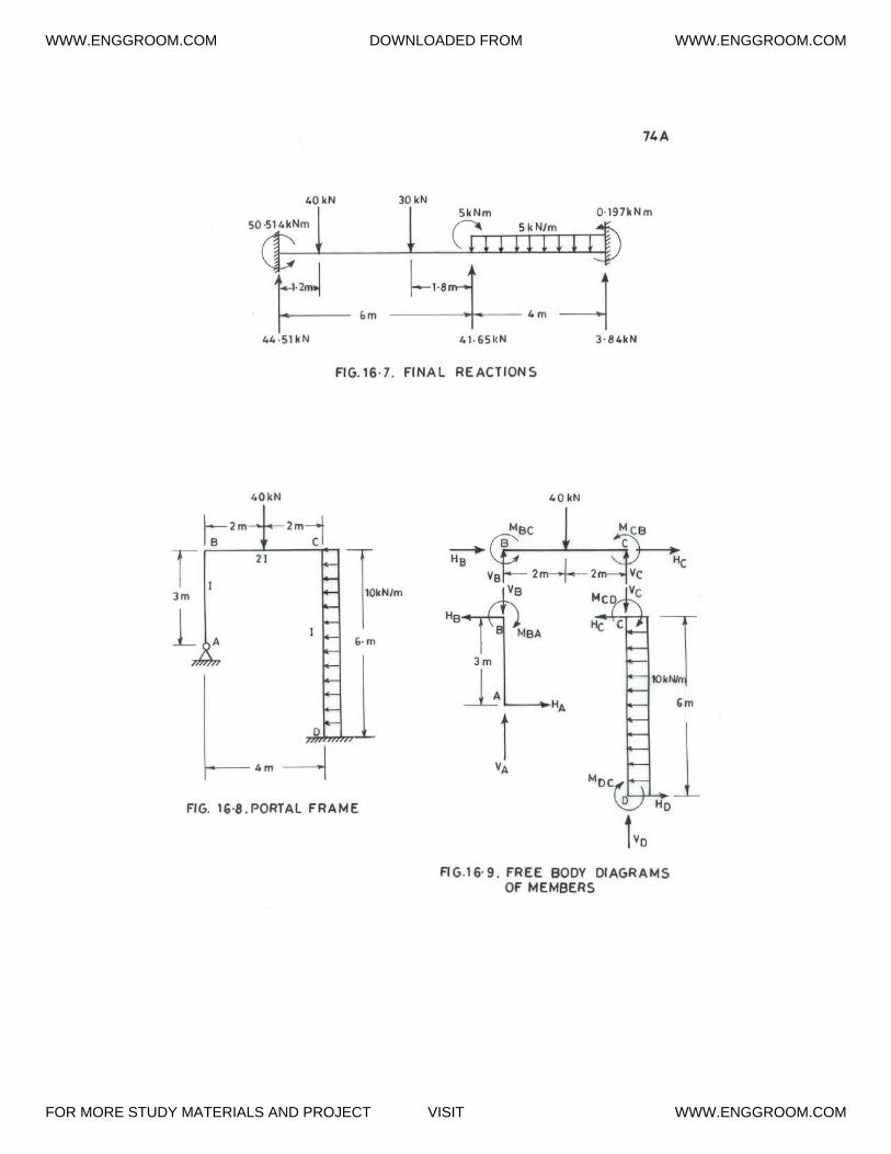
WWW.ENGGROOM.COM DOWNLOADED FROM WWW.ENGGROOM.COM
FOR MORE STUDY MATERIALS AND PROJECT VISIT WWW.ENGGROOM.COM

-75-
Numerical example on portal frame
A portal frame loaded as shown in figure 16.8 is analyzed for member end forces by
slope-deflection method.
DOF = 4 (θA, θB, θC, Δ)
Rotations are taken positive clockwise at the joints and lateral displacement Δ at the
beam level is taken positive to left.
Since A is a hinge : MAB = 0
Since D is clamp θD = 0
MFBC = - 4x 4
2 x 2 x 2 x 40= - 20 kNm
MFCB = + 8
4 x 40 = + 20 kNm
MFAB = MFBA = 0
MFCD = - 12
6 x 6 x 10= - 30 kNm
MFDC = + 12
6 x 6 x 10= + 30 kNm
MAB = + ⎟⎠⎞
⎜⎝⎛ Δ
++3
32
3
EI 2BA θθ
MBA = + ⎟⎠⎞
⎜⎝⎛ Δ
++3
32
3
EI 2BA θθ
MBC = - 20 + ( )CB24
EI 4 θθ +
MCB = + 20 + ( )CB 24
EI 4 θθ +
MCD = - 30 + ⎟⎠⎞
⎜⎝⎛ Δ
++6
302
6
EI 2Cθ
WWW.ENGGROOM.COM DOWNLOADED FROM WWW.ENGGROOM.COM
FOR MORE STUDY MATERIALS AND PROJECT VISIT WWW.ENGGROOM.COM

-76-
MDC = + 30 + ⎟⎠⎞
⎜⎝⎛ Δ
++6
30
6
EI 2Cθ
The unknown displacements θA, θB, θC and Δ can be obtained from three moment
equilibrium equations of joints and one shear equilibrium equation.
MAB = 0 ------------------ (1)
MBA + MBC = 0 --------- (2)
MCB + MCD = 0 --------- (3)
HA + HD – 60 = 0 ------- (4)
HA = 3
MBA
HD = 6
3 x 60MM DCCD ++
2 MBA + MCD + MDC = 180 ---- (4)
⎟⎠⎞
⎜⎝⎛ Δ
++3
32
3
2EIBA θθ = 0
θA = - 22
B Δ−
θ ------------------ (1)
( )Δ++ BA 23
2EI θθ - 20 + EI (2θB + θC) = 0
2θA + 4θB + 2Δ + 6θB + 3θC = EI
60
3θC + 10θB + 2θA + 2Δ = EI
60--- (2)
20 + EI (θB + 2θC) – 30 + ⎟⎠⎞
⎜⎝⎛ Δ
+2
23
EICθ = 0
WWW.ENGGROOM.COM DOWNLOADED FROM WWW.ENGGROOM.COM
FOR MORE STUDY MATERIALS AND PROJECT VISIT WWW.ENGGROOM.COM

-77-
6θB + 12θC + 4θC + Δ = +EI
60
6θB + 16θC + Δ = EI
60+--------- (3)
( ) ⎟⎠⎞
⎜⎝⎛ Δ
+++⎟⎠⎞
⎜⎝⎛ Δ
++−Δ++23
EI30
22
3
EI302
3
4EICCBA θθθθ = 180
4θA + 8θB + 3θC + 5Δ = EI
540----- (4)
Substituting value of θA from equation (1) in equations (2) and (4):
3θC + 9θB + Δ = EI
60--------- (5)
6θB + 3θC + 3Δ = EI
540----- (6)
or 2θB + θC + Δ = EI
180----- (6)
Eqn (5) – Eqn (6) gives:
7θB + 2θC = EI
120----------- (7)
Eqn (3) – Eqn (6) gives:
4θB + 15θC = - EI
120----------- (8)
Equations (7) & (8) are solved for θB and θC.
(8θC + 105θC) = - EI
480+
EI
840=
EI
360
θC = - EI
711.3
97EI
360−=
WWW.ENGGROOM.COM DOWNLOADED FROM WWW.ENGGROOM.COM
FOR MORE STUDY MATERIALS AND PROJECT VISIT WWW.ENGGROOM.COM

-78-
θB = EI
082.16
97EI
360 x 15
EI
120
4
1 −=⎥⎦
⎤⎢⎣⎡ +−
From eqn (6), we get Δ and from eqn (1) θA
Δ = EI
180+ 2 x
EI
082.16 +
EI
711.3=
EI
875.215
θA = -2EI
875.215 +
2EI
082.16 = -
EI
897.99
Now member end moments are computed from slope deflection equations.
MAB = 3
2EI ⎥⎦
⎤⎢⎣⎡ +−
EI
875.215
EI
082.16
EI
99.897 -x 2 = 0 (check)
MBA = 3
EI2 ( )⎥⎦⎤
⎢⎣⎡ ++
EI
875.215
EI
16.082 -x 2
EI
99.897 - = 55.876 kNm
MBC = - 20 + EI ( )
⎥⎦⎤
⎢⎣⎡ −
EI
711.3
EI
16.082 -x 2= - 55.875 kNm
MCB = 20 + EI ⎥⎦⎤
⎢⎣⎡ −
EI
711.3x 2
EI
16.082 -= - 3.504 kNm
MCD = - 30 + 3
EI⎥⎦⎤
⎢⎣⎡ +−
2EI
875.215
EI
711.3x 2= + 3.505 kNm
MDC = 30 + 3
EI⎥⎦⎤
⎢⎣⎡ +−
2EI
875.215
EI
711.3 = 64.742 kNm
Shears and axial forces at the ends of members are computed from free body diagrams of
members shown in Figure 16.9.
Member AB
HA = HB = 3
876.55= 18.625 kN
WWW.ENGGROOM.COM DOWNLOADED FROM WWW.ENGGROOM.COM
FOR MORE STUDY MATERIALS AND PROJECT VISIT WWW.ENGGROOM.COM

-79-
Member BC
HC = - HB = - 18.625 kN
VB = 2
40+ ( )
4
504.3875.55 += 34.845 kN
VC = 2
40- ( )
4
504.3875.55 += 5.155 kN
Member CD
VD = VC = 5.155 kN
HD = 6
3.505 64.742 3 x 6x 10 ++= 41.375 kN
Member AB
VA = VB = 34.845 kN
VA + VD = 40 kN, HA + HD = 60 kN (check)
17 ANALYSIS OF INDETERMINATE TRUSSES
External indeterminacy of a truss is computed as follows.
E∝ = R – r
E∝ = External indeterminacy
R = Total number of reaction components
r = Minimum number of equilibrium equations for truss as a whole for stability.
For plane truss:
∝I = m – (2j – r)
∝I = Internal indeterminacy
WWW.ENGGROOM.COM DOWNLOADED FROM WWW.ENGGROOM.COM
FOR MORE STUDY MATERIALS AND PROJECT VISIT WWW.ENGGROOM.COM

-80-
m = total number of members
j = total number of joints
∝S = Total statical indeterminacy of truss
∝S = E∝ + ∝I = (m + r – 2j)
For space truss:
∝S = (m + R – 3j)
∝I = m – (3j – r)
Internally redundant truss to first degree
Shown in figure 17.1 is internally indeterminate truss to first degree. It is made
determinate by removing one member as shown in figure 17.2.
Fi = Force in ith member of determinate truss due to given external loads.
m = number of members in determinate truss
Li = Length of ith member
Ai = area of cross section of ith member
X = Force in member which has been removed from redundant truss due to external loads
acting on indeterminate truss as shown in figure 17.3.
ki = Force in ith member of determinate truss due to unit actions corresponding to
member removed as shown in figure 17.4.
iF = Total force in ith member due to external loads and the forces X corresponding to
removed member.
iF = Fi + ki X
U = strain energy of determinate truss due to external loads and force X.
( )∑=
+=
m
1i i
i
2
ii
E2A
LXkF U
WWW.ENGGROOM.COM DOWNLOADED FROM WWW.ENGGROOM.COM
FOR MORE STUDY MATERIALS AND PROJECT VISIT WWW.ENGGROOM.COM

WWW.ENGGROOM.COM DOWNLOADED FROM WWW.ENGGROOM.COM
FOR MORE STUDY MATERIALS AND PROJECT VISIT WWW.ENGGROOM.COM
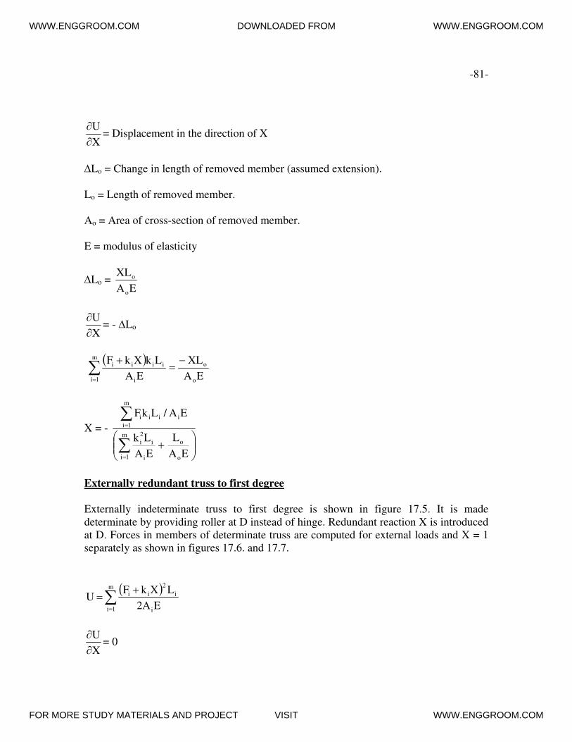
-81-
X
U
∂∂
= Displacement in the direction of X
ΔLo = Change in length of removed member (assumed extension).
Lo = Length of removed member.
Ao = Area of cross-section of removed member.
E = modulus of elasticity
ΔLo = EA
XL
o
o
X
U
∂∂
= - ΔLo
( )EA
XL
EA
LkXkF
o
om
1i i
iiii −=
+∑=
X = -
⎟⎟⎠
⎞⎜⎜⎝
⎛+∑
∑
=
=m
1i o
o
i
i
2
i
m
1i
iiii
EA
L
EA
Lk
EA/LkF
Externally redundant truss to first degree
Externally indeterminate truss to first degree is shown in figure 17.5. It is made
determinate by providing roller at D instead of hinge. Redundant reaction X is introduced
at D. Forces in members of determinate truss are computed for external loads and X = 1
separately as shown in figures 17.6. and 17.7.
( )∑=
+=
m
1i i
i
2
ii
E2A
LXkF U
X
U
∂∂
= 0
WWW.ENGGROOM.COM DOWNLOADED FROM WWW.ENGGROOM.COM
FOR MORE STUDY MATERIALS AND PROJECT VISIT WWW.ENGGROOM.COM

-82-
( )∑=
+m
1i i
iiii
EA
LkXkF = 0
X = -
∑
∑
=
=m
1i i
i
2
i
m
1i i
iii
EA
LK
EA
LkF
Trusses with n-degrees of redundancy
The truss is made determinate by removing redundant members and reactions. The
determinate truss is analyzed for forces in members due to given external loads and due
to unit redundant forces X1, …. Xj, …., Xn.
kij = Force in member I due to Xj = 1 in determinate truss.
iF = Fi + ∑=
n
1j
ijk Xj
The strain energy of the truss including strain energy of redundant members is given by:
E2A
LX
E2A
LXkF
Uj
j
2
jm
1i i
i
2
j
n
1j
iji
+⎟⎟⎠
⎞⎜⎜⎝
⎛+
=∑∑
=
=
Lj = Length of member corresponding to redundant member.
For strain energy to be minimum.
1X
U
∂∂
= 2X
U
∂∂
= ….. jX
U
∂∂
= ……… = nX
U
∂∂
= 0
For unknown forces corresponding to redundant members:
jX
U
∂∂
= EA
LX
EA
LkXkF
j
jjm
1i i
iij
n
1j
ij
+⎟⎟⎠
⎞⎜⎜⎝
⎛+
∑∑
=
= = 0
WWW.ENGGROOM.COM DOWNLOADED FROM WWW.ENGGROOM.COM
FOR MORE STUDY MATERIALS AND PROJECT VISIT WWW.ENGGROOM.COM

-83-
For unknown forces corresponding to reactions Lj is set equal to zero. The partial
derivatives with respect to all the n-unknowns give a system of simultaneous equations,
which is solved for unknowns and the forces in indeterminate truss.
Lack of fit in members of indeterminate trusses
No forces are generated in members of determinate truss due to lack of fit but in case of
indeterminate truss the forces are generated in members when the members with lack of
fit are forced into position. Consider an indeterminate truss ABCD in which member BC
is shorter than its exact length by amount δ as shown in figure 17.8. The member will
come in tension when fitted.
X = force in member due to lack of fit.
System is made determinate by removing members having lack of fit. Unit forces X = 1
are applied as shown in figure 17.9.
iF = kiX
( )∑=
=m
1i i
i
2
i
EA
LXk U
δ = X
U
∂∂
= movement in the direction of force
δ+−=∑
= EA
XL
EA
XLk
o
om
1i i
i
2
i
Lo = Length of member having lack of fit
Ao = Area of member having lack of fit
X =
⎟⎟⎠
⎞⎜⎜⎝
⎛+∑
=
m
1i o
o
i
i
2
i
EA
L
EA
Lk
δ
If member with lack of fit is longer than Lo, δ will be taken negative.
WWW.ENGGROOM.COM DOWNLOADED FROM WWW.ENGGROOM.COM
FOR MORE STUDY MATERIALS AND PROJECT VISIT WWW.ENGGROOM.COM

WWW.ENGGROOM.COM DOWNLOADED FROM WWW.ENGGROOM.COM
FOR MORE STUDY MATERIALS AND PROJECT VISIT WWW.ENGGROOM.COM

-84-
Temperature forces in redundant trusses
The member BC is subjected to rise in temperature of ΔToC.
δLo = ∝Lo ΔT
∝ = Coefficient of thermal expansion
The truss is made determinate by removing the member which is subjected to
temperature change. Unit loads are applied at the joints of the member as shown in figure
17.10. and forces in various members are computed.
Force in redundant member BC = kX
( )∑=
=m
1i i
i
2
i
E2A
LXk U
X
U
∂∂
= movement in the direction of force X
EA
XL - TL
EA
XLL
EA
XLk
o
oo
o
oo
m
1i i
i
2
i Δ∝=−=∑=
δ
X =
⎟⎟⎠
⎞⎜⎜⎝
⎛+
Δ∝
∑=
m
1i o
o
i
i
2
i
o
EA
L
EA
Lk
T L
If member BC is subjected to fall in temperature ΔT will be taken negative.
The method discussed above is applicable to plane as well as space trusses and pertains to
force method.
Numerical examples
Example 17.1.
For the cantilever truss shown in figure 17.11 find the forces in members. The axial
rigidity AE of all the members is same.
WWW.ENGGROOM.COM DOWNLOADED FROM WWW.ENGGROOM.COM
FOR MORE STUDY MATERIALS AND PROJECT VISIT WWW.ENGGROOM.COM

-85-
There are three members meeting at joint A and two equations of equilibrium, hence,
static indeterminacy is 1. Let AC be redundant member. It is removed to obtain
determinate system as shown in figure 17.12.
Joint A
F1 Sin 45o + F3 Sin 30
o = 1000
F1 Cos 45o = F1 Cos 30
o
F1 = 2
23 F3 =
2
3 F3
⎟⎟⎠
⎞⎜⎜⎝
⎛+
2
1
2
3 F3 = 1000
F3 = ( )13
2000
+ = 732.051 (comp)
F1 = 896.576 (Tension)
We apply unit actions corresponding to unknown tensile force in AC as shown in figure
17.13.
Joint A
k1 Sin 45o = k3 Sin 30
o
k3 = 2 k1
k1 Cos 45o = k3 Cos 30
o = 1
22
3
2
k1 + k1 = 1
k1 ( ) 231 =+
WWW.ENGGROOM.COM DOWNLOADED FROM WWW.ENGGROOM.COM
FOR MORE STUDY MATERIALS AND PROJECT VISIT WWW.ENGGROOM.COM

-86-
k1 = ( ) 7321.2
4142.1
31
2=
+ = 0.518 (comp)
k3 = ( )31
2
+ = 0.732 (comp)
X = -
⎟⎟⎠
⎞⎜⎜⎝
⎛+∑
∑
=
=
1,3i o
o
i
i
2
i
1,3i i
iii
EA
L
EA
Lk
EA
LkF
= - o3
2
31
2
1
333111
LLk Lk
LkFLkF
+++
X = -
( ) ( )( )
( ) ( ) L L3
20.732 - L20.518 -
L3
2732.0732.051 - L20.518 -x 576.896
22 ++
−+
X = - ( )( ) 998.1
039.38
1 0.619 0.379
618.759 656.798 -=
+++
= 19.039 kN
1F = F1 + k1 X = 896.576 – 0.518 x 19.039 = 886.714 kN
2F = X = 19.039 kN
3F = F3 + k3 X = - 732.051 – 0.732 x 19.039 = - 745.988 kN
The final forces in members are shown in figure 17.14.
Check
x – direction
- 19.039 + 745.988 x 2
3 - 886.714 x
2
1 = - 19.039 + 646.045 – 627.001 = 0.004 (ok)
WWW.ENGGROOM.COM DOWNLOADED FROM WWW.ENGGROOM.COM
FOR MORE STUDY MATERIALS AND PROJECT VISIT WWW.ENGGROOM.COM

-87-
y-direction
886.714 x 2
1 + 745.988 x
2
1- 1000 = 627.001 + 372.994 – 1000 = 0 (ok)
It can be seen that there are small computational errors as the forces are not summing up
to zero exactly. However, residuals are small and neglected.
Example 17.2.
For internally indeterminate truss shown in figure 17.15 determine forces in all members.
E = 200 kN/mm2
Size of vertical members = 30 x 20 mm
Size of horizontal members = 30 x 30 mm
Size of diagonal members = 20 x 20 mm
Member BC is removed to make the truss determinate as shown in figure 17.16. Forces
in members F are now determined.
RAV = RD = 7.5 kN
RAH = 10 kN
Joint C
F4 Cos θ = 10
F4 = 10 x 4
50
4
5= = 12.5 kN (Tension)
F2 = F4 Sin θ = 2
15
5
3x
4
50= = 7.5 kN (comp)
Joint B
F1 = F5 = 0
WWW.ENGGROOM.COM DOWNLOADED FROM WWW.ENGGROOM.COM
FOR MORE STUDY MATERIALS AND PROJECT VISIT WWW.ENGGROOM.COM

WWW.ENGGROOM.COM DOWNLOADED FROM WWW.ENGGROOM.COM
FOR MORE STUDY MATERIALS AND PROJECT VISIT WWW.ENGGROOM.COM

-88-
Joint A
F3 = 10 – F4 Cos θ = 10 - 5
4x
4
50= 0
Now unit actions are applied at B and C as shown in figure 17.17 and forces are
determined in members.
Joint B
k5 Cos θ = 1, k5 = 4
5= 1.25 kN (comp)
k1 = k5 Sin θ = 4
3
5
3x
4
5= = 0.75 kN (Tension)
Joint A
k4 Sin θ = k1 = 4
3
k4 = 4
5
4
3x
3
5= kN (comp)
k3 = k4 Cos θ = 5
4x
4
5= 1 kN (Tension)
Joint C
K2 = k4 Sin θ = 4
3
5
3x
4
5= = 0.75 kN (Tension)
X = -
∑
∑
∑
∑
+
−=
+o
o
2
o
o
2
A
L
A
Lk
A
FkL
EA
L
AE
Lk
AE
FkL
WWW.ENGGROOM.COM DOWNLOADED FROM WWW.ENGGROOM.COM
FOR MORE STUDY MATERIALS AND PROJECT VISIT WWW.ENGGROOM.COM

-89-
Computations are carried out in tabular form
Member Force F
(kN)
Force k
(kN)
Length
(mm)
Area
(mm2) A
FkL
A
Lk 2
Final Force F
(F + k X)
1
2
3
4
5
0
-7.5
0
12.5
0
0.75
0.75
1.00
-1.25
-1.25
3000
3000
4000
5000
5000
600
600
900
400
400
0
- 28.125
0
-195.312
0
2.8125
2.8125
4.4444
19.5312
19.5312
3.128
- 4.373
4.170
7.288
- 5.213
∑ -223.437 49.1318
900
4000
A
L
o
o = = 4.44444
X = - ( )4444.41318.49
437.223
+−
= + 4.17 kN
18 APPROXIMATE METHODS OF ANALYSIS OF
STATICALLY INDETERMINATE STRUCTURES
Even the so called exact analysis of structures is approximate in the broad sense because
every analysis is based on assumptions with respect to geometry and material behavior of
structure. However, the approximate analysis for statically indeterminate structures is
based on assumptions, which render the indeterminate system to a determinate system,
which can be analyzed exactly by use of equations of equilibrium. The advantage is that
analysis of determinate systems does not depend on elastic properties of members where
as analysis of statically indeterminate systems depends on elastic properties of members.
Approximate analysis is also required for assumption of initial elastic properties of
members in order to carry out design of indeterminate structure. Approximate methods
are also adopted under situation of configuration complexity of structure for which exact
method of analysis is not available. Where exact analysis requires prohibitive time and
cost it should be abandoned and approximate method adopted which generally gives
conservative design. The first step in approximate analysis of statically indeterminate
structure is to determine its statical indeterminacy and then introduce equal number of
releases to make it determinate.
WWW.ENGGROOM.COM DOWNLOADED FROM WWW.ENGGROOM.COM
FOR MORE STUDY MATERIALS AND PROJECT VISIT WWW.ENGGROOM.COM

-90-
The following types of statically indeterminate structures are generally analyzed by
approximate methods.
1. Parallel chord trusses with two diagonals in each panel.
2. Portals, trussed portals and mill bents.
3. Towers with straight legs.
4. Building frames.
The approximate analysis will be explained on following examples.
1. Parallel chord indeterminate truss shown in figure 18.1.
The degree of static indeterminacy is 4 as four additional diagonal members have
been introduced in just rigid or determinate simple truss. The assumption that will be
made here is that in each panel the shear is equally divided between the two diagonals
or in other words the numerical values of force in diagonal members of same panel
are equal. This amounts to four independent assumptions or reduction of static
indeterminacy by 4, hence, truss can be analyzed as determinate truss.
2. Fixed portal under horizontal load.
For the portal shown in figure 18.2 the degree of static indeterminacy is 3. Hence,
three assumptions are required. The points of contra flexure occur at mid height of
columns. Hence, two hinges will be introduced at mid height as shown in Figure 18.3.
The third assumption will be made as equal resistance to shear by the columns. Now
analysis is possible by equations of equilibrium and is self explanatory from figure
18.4.
3. Trussed portal and mill bents.
Here also, the hinges are introduced at mid height of columns and it is assumed that
columns carry same horizontal shear as shown in figures 18.5 and 18.6.
Vertical reaction at hinges = L
h2
H P ⎟
⎠⎞
⎜⎝⎛ +
Other results are self explanatory.
WWW.ENGGROOM.COM DOWNLOADED FROM WWW.ENGGROOM.COM
FOR MORE STUDY MATERIALS AND PROJECT VISIT WWW.ENGGROOM.COM

WWW.ENGGROOM.COM DOWNLOADED FROM WWW.ENGGROOM.COM
FOR MORE STUDY MATERIALS AND PROJECT VISIT WWW.ENGGROOM.COM

-91-
4. Tower with straight legs shown in figure 18.7.
Tower is a space truss. For approximate analysis it is necessary that each face of
tower should be a plane. Each face is separated out as a plane truss as shown in figure
18.8 and equivalent inplane loads are shown. The indeterminate plane truss is
replaced by two determinate plane trusses as shown figures 18.9 and 18.10 and the
loads are apportioned on these trusses. Final result of forces in the members is
obtained by superposing the results of individual trusses.
5. Plane multistory indeterminate frames as shown in figure 18.11.
The analysis is carried out separately for vertical and lateral loads. For lateral loads
following methods are used.
(1) Portal method
(2) Cantilever method
(3) Factor method
Analysis for vertical loads
The analysis for vertical loads is carried out on following assumptions
(a) The axial force in the girder is zero
(b) A point of inflection occurs in the girder at one-tenth point measured along span from
each end. The hinges are introduced at these points as shown in figure 18.12.
(c) The girder is analyzed for positive BM as a simply supported beam of span 0.8L and
the vertical reactions are transferred to cantilever parts of span 0.1L as shown in
Figure 18.13. The negative moments at the ends of beam are computed as the
negative moments at the cantilever clamps as shown in figure 18.14. The vertical
reactions of clamps are transferred to the columns as axial loads.
(d) At the beam column junction the clamp bending moment is distributed between the
columns above and below in proportion to their stiffness. A typical girder AB is
considered as shown in figure 18.15.
Maximum positive BM at centre = ( )
8
L8.0 2ω
= 0.08 ωL2.
Maximum reaction at hinge = 0.4ωL.
WWW.ENGGROOM.COM DOWNLOADED FROM WWW.ENGGROOM.COM
FOR MORE STUDY MATERIALS AND PROJECT VISIT WWW.ENGGROOM.COM

WWW.ENGGROOM.COM DOWNLOADED FROM WWW.ENGGROOM.COM
FOR MORE STUDY MATERIALS AND PROJECT VISIT WWW.ENGGROOM.COM

WWW.ENGGROOM.COM DOWNLOADED FROM WWW.ENGGROOM.COM
FOR MORE STUDY MATERIALS AND PROJECT VISIT WWW.ENGGROOM.COM

-92-
Maximum negative bending moment is computed as cantilever clamp moment.
Maximum negative BM at end MA = ω(0.1L) ( )
2
L1.0 + 0.4ωL (0.1L) = 0.045 ωL
2
Reaction at end A RA = ω(0.1L) + 0. 4ωL = 0.5 ωL
At A axial load transmitted to column is RA = 0.5 ωL.
The moment MA is distributed to upper and lower columns proportional to their
stiffnesses.
MAU = MA ( )21
2
KK
K
+
MAL = MA ( )21
1
KK
K
+
If at the joint their is beam on the other side also, its analysis can also be carried out
similarly and forces in column superposed.
Analysis for horizontal loads
Portal Method
In portal method following assumptions are made.
(a) The point of contra flexure in each girder is located at its mid span point.
(b) The point of contra flexure in a column is located at mid height of each column.
(c) The total horizontal external shear on each storey is distributed between the column
of that storey so that each interior column carries twice as much shear as the exterior
column.
Shown in figure 18.16 is a plane frame with columns C1 to C6 and girders g1 to g4. It is
subjected to lateral loads P and Q. The hinges are assumed at mid points of all the
members and the horizontal shears are distributed in columns in accordance with the
rules as shown in figure 18.17.
WWW.ENGGROOM.COM DOWNLOADED FROM WWW.ENGGROOM.COM
FOR MORE STUDY MATERIALS AND PROJECT VISIT WWW.ENGGROOM.COM

WWW.ENGGROOM.COM DOWNLOADED FROM WWW.ENGGROOM.COM
FOR MORE STUDY MATERIALS AND PROJECT VISIT WWW.ENGGROOM.COM

-93-
BM in column
BM in a column is equal to shear in column multiplied by half its height.
BM in C1 = ( )
4
HQ P
2
H
2
Q P 11 +=⎟
⎠⎞
⎜⎝⎛ +
BM in C2 = ( )
4
PH2
BM in girder
The girder and column moments act in apposite directions at their junction in accordance
with their elastic line or deflection curve as shown in figure 18.18.
At joint E:
MC1 + MC2 = Mg1 + Mg2
Since column end moments are now known the beam end moments can be computed. At
end F of g2:
MFE = MC5 + MC6
Since moment at centre of girder is zero, Mg2 = MFE.
Hence, Mg1 = MC1 + MC2 – Mg2.
Thus proceeding across the girder of first level the girder moments are determined. The
girder moments at other level can also be determined in the same manner.
SF in girder
Considering free body of g2, as shown in figure 18.19 the shear at ends is obtained
Vg2 = 2
g2
L
M2
Likewise shear is determined in all girders.
WWW.ENGGROOM.COM DOWNLOADED FROM WWW.ENGGROOM.COM
FOR MORE STUDY MATERIALS AND PROJECT VISIT WWW.ENGGROOM.COM

-94-
AF in columns
Axial forces in columns can be obtained by summing up from the top of the column, the
shears transferred to the column by the girders connected to this column.
AF in girder
Axial forces in girders are obtained by summing up the horizontal forces from one end of
the girder to the other end.
Cantilever method
The following assumptions are made.
1) As in portal method the points of contra flexure are assumed at mid points of all
beams and columns as shown in figure 18.20.
2) The intensity of axial stress in each column of a storey is proportional to the
horizontal distance of that column from the centre of gravity of all columns of that
storey. The steps of this method are demonstrated on a three by two plane frame as
shown in figure 18.20. It is assumed that all columns have same area of cross-section
A. The distance of CG of columns x in horizontal direction from A is computed as
follows as shown in figure 18.21.
x (4A) = AL1 + A(L1 + L2) + A(L1 + L2 + L3)
x = ( )
4
LL23L 321 ++
FAE = axial force in AE (T)
FBF = Axial force in BF = ( )
x
L -x 1 FAE (T)
FCG = Axial force in CG = ( )
x
xLL 21 −+ FAE (C)
FDH = Axial force in DH = ( )
x
xLLL 321 −++FAE (C)
Taking a free body above the horizontal section through mid points of columns of first
storey the expression for moment about mid point of column DH is set equal to zero.
WWW.ENGGROOM.COM DOWNLOADED FROM WWW.ENGGROOM.COM
FOR MORE STUDY MATERIALS AND PROJECT VISIT WWW.ENGGROOM.COM
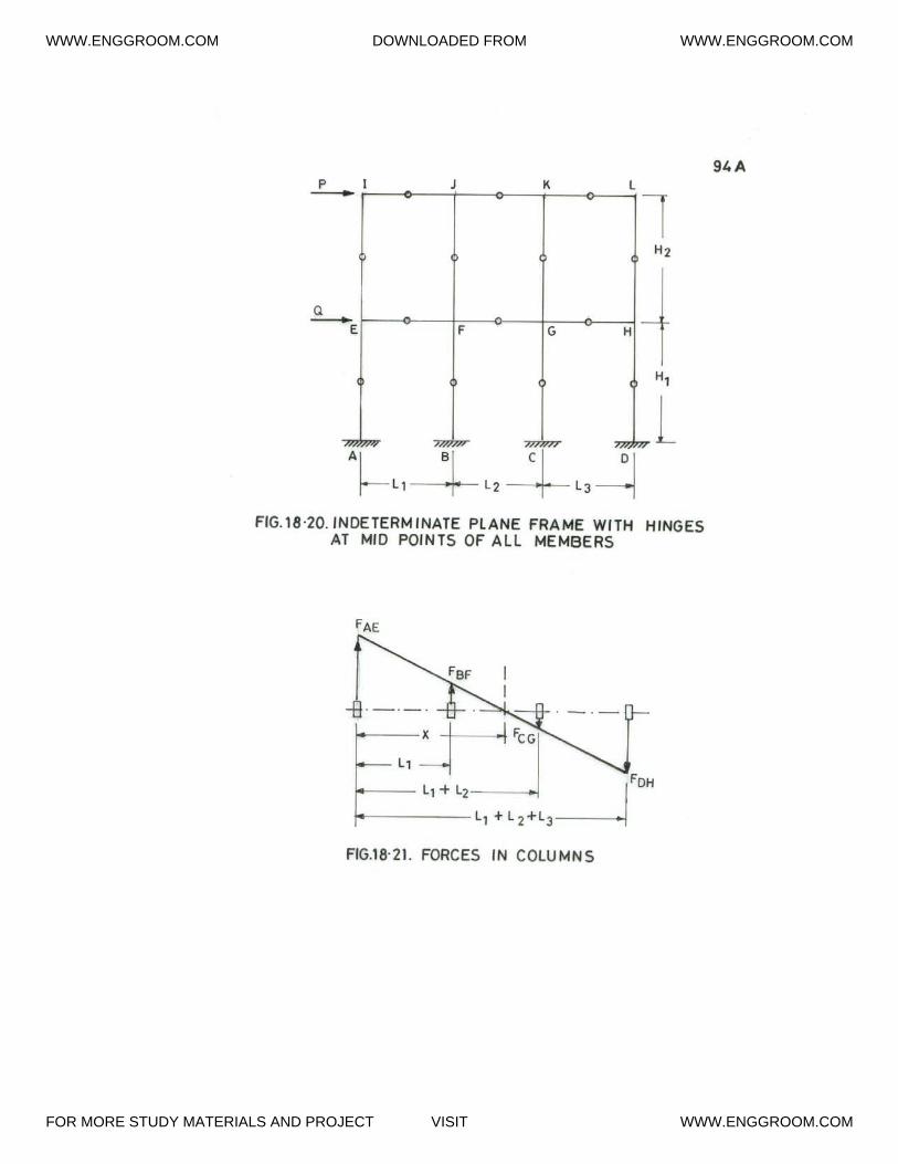
WWW.ENGGROOM.COM DOWNLOADED FROM WWW.ENGGROOM.COM
FOR MORE STUDY MATERIALS AND PROJECT VISIT WWW.ENGGROOM.COM

-95-
P ⎟⎠⎞
⎜⎝⎛ +
2
HH 1
2 + Q ⎟⎠⎞
⎜⎝⎛
2
H1 - FAE (L1 + L2 + L3) - x
FAE (x – L1) (L2 + L3)
+ x
FAE (L1 + L2 - x) L3 = 0
This gives the value of FAE, hence, forces in columns of first storey are computed. The
forces in columns of second storey are computed in the same manner by taking moment
about mid point of column HL of the free body above the horizontal section through mid
points of columns of second storey.
Girder shears
The girder shears can be obtained from the column axial forces at the various joints as
shown in figure 18.22.
Joint I
VIJ = FIE
Joint E
VEF = FEA – VIJ = FEA – FIE
Girder moments
The moment at each end of girder equals the shear in that girder multiplied by half the
length of that girder as shown in figure 18.23. For example:
MEF = VEF 2
L1
Column moments
Column moments are determined by beginning at the top of each column stack and
working progressively down to base as shown in figure 18.24.
Joint J
MJF = VIJ 2
L1 + VJK 2
L2
WWW.ENGGROOM.COM DOWNLOADED FROM WWW.ENGGROOM.COM
FOR MORE STUDY MATERIALS AND PROJECT VISIT WWW.ENGGROOM.COM

WWW.ENGGROOM.COM DOWNLOADED FROM WWW.ENGGROOM.COM
FOR MORE STUDY MATERIALS AND PROJECT VISIT WWW.ENGGROOM.COM

-96-
Since there is a point of contra flexure at the center of FJ, MFJ will be equal to MJF.
MFJ = MJF
MFB + MFJ = MFG + MFE
MFB = MFG + MFE - MFJ
Because of hinge in middle of column:
MBF = MFB
Proceeding in this manner moments, shears and axial forces in all members are
determined.
The factor method
This method is more accurate compared to portal and cantilever methods. The
assumptions in factor method are based on elastic action of structure hence results of this
method correspond to approximate slope-deflection analysis. The method is not discussed
here.
*** CONCLUDING REMARKS ***
Readers are welcome to point out any errors noticed in the lecture course material
so that corrections can be incorporated. Any suggestions are welcome by the author.
WWW.ENGGROOM.COM DOWNLOADED FROM WWW.ENGGROOM.COM
FOR MORE STUDY MATERIALS AND PROJECT VISIT WWW.ENGGROOM.COM