Embed Size (px)
Citation preview

Financial Data Analysis
Dr. Markus Haas
LMU Munchen
Summer term 2010
April 21, 2010

Financial Data Analysis
• Markus Haas, [email protected] hour: Tuesday 16-18 and by appointment
• Prerequisites: “Einfuhrung in die Empirische Wirtschaftsforschung”,“Okonometrie1” or ”Applied Econometrics”
1
Course Outline
• Introduction: Basic properties of financial return series
• Review of linear time series methods
• Parametric volatility modeling
(i) GARCH(ii) Stochastic volatility models(iii) Regime–switching models
• Modeling the dependence structure of returns
(i) Multivariate GARCH processes(ii) Multivariate regime–switching and copulas
• Value–at–Risk: Regulatory framework, quantile estimation, backtesting
2

Textbooks
• Taylor, S. (2005), Asset Price Dynamics, Volatility, and Prediction,Princeton University Press, New Jersey.
• Alexander, C. (2008), Practical Financial Econometrics, Wiley, New York
• Tsay, R.S. (2005), Analysis of Financial Time Series, 2e, Wiley, NewYork.
• Malevergne, Sornette (2006), Extreme Financial Risks, From Dependenceto Risk Management, Springer, Berlin. (For copulas)
• Hamilton (1994), Time Series Analysis, Princeton University Press,Princeton, New Jersey.
• Mills, T. C., Markellos (2008), The Econometric Modelling of FinancialTime Series, 2e, Cambridge University Press.
• Campbell, Lo, and MacKinlay (1997), The Econometrics of FinancialMarkets, Princeton University Press.
3
• Franses, van Dijk (2000), Non–Linear Time Series Models in EmpiricalFinance, Cambridge University Press.
4
Returns
• Let Pt be the asset price at time t.
• There is a dividend payment Dt at the end of period t.
• Then the (single–period) discrete return is
Rt =Pt + Dt − Pt−1
Pt−1. (1)
• Dividends are often excluded from return calculations.
• Often (1) is multiplied by 100 to be interpretable in terms of percentagereturns.
• The continuously compounded or log return is (ignoring dividends forsimplicity)
rt = log Pt − log Pt−1 = log(1 + Rt). (2)
5

• This name derives from the fact that the interest rate in equivalent toRt, when interest is paid n times in the period, solves
(1 +
inn
)n
= 1 + Rt. (3)
• Continuous compounding is approached as n →∞, and then
ei∞ = 1 + Rt ⇒ i∞ = log(1 + Rt) = rt. (4)
• Empirical analysis is often based on log returns. These have theadvantage that they can be additively aggregated over time.
• That is, if rt,t+τ denotes the (multi–period) return from time t to timet + τ , we have
rt,t+τ = log(
Pt+τ
Pt
)=
τ∑
i=1
rt+i. (5)
6

• This is not the case for the discrete return, where
Rt,t+τ =τ∏
i=1
(1 + Rt+i)− 1. (6)
• On the other hand, if we consider a portfolio of N assets with weightsai, and returns Rit, i = 1, . . . , n, then the portfolio return is
Rp,t =N∑
i=1
aiRit, (7)
whereas
rp,t = log(1 + Rp,t) 6=N∑
i=1
airit, (8)
i.e., the linear combination of continuously compounded asset returns isnot the continuously compounded portfolio return.
7

• For small x,1
log(1 + x) = x− x2
2+
x3
3− x4
4+ · · · ≈ x, (9)
so that rt may serve as a reasonable approximation to the discrete return.
Table 1: Discrete and continuous returns100× Rt -30.0 -20.0 -15.0 -10.0 -5.0 0 5.0 10.0 15.0 20.0 30.0
100× rt -35.7 -22.3 -16.3 -10.5 -5.1 0 4.9 9.5 14.0 18.2 26.2
Rt and rt = log(1 + Rt) are the discrete and continuously compounded returns, respectively.
• The approximation
rp,t ≈N∑
i=1
airit (10)
is also frequently used.
1Note that the expansion (not the approximation) is only valid for x ∈ (−1, 1].
8

Basic Statistical Properties of Returns: ReturnDistribution
• The traditional assumption that has long dominated empirical finance wasthat log–returns over longer time intervals are approximately normallydistributed.
• For example, daily returns are the sum of a large number of intradayreturns.
• Appealing to the central limit theorem, Osborne (1959) argued in aclassical article that2
“under fairly general conditions [...] we can expect that the distributionfunction of [rt] will be normal.”
2Brownian Motion in the Stock Market, Operations Research 7, 145-173.
9
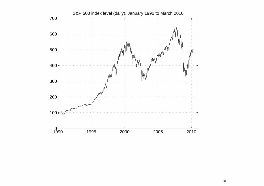
1990 1995 2000 2005 20100
100
200
300
400
500
600
700S&P 500 index level (daily), January 1990 to March 2010
10
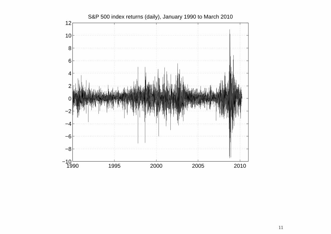
1990 1995 2000 2005 2010−10
−8
−6
−4
−2
0
2
4
6
8
10
12S&P 500 index returns (daily), January 1990 to March 2010
11

1990 1992 1994 1996 1998 2000 2002 2004 2006 2008 2010−10
−8
−6
−4
−2
0
2
4
6
8
10
12DAX 30 index returns (daily), January 1990 to October 2009
12
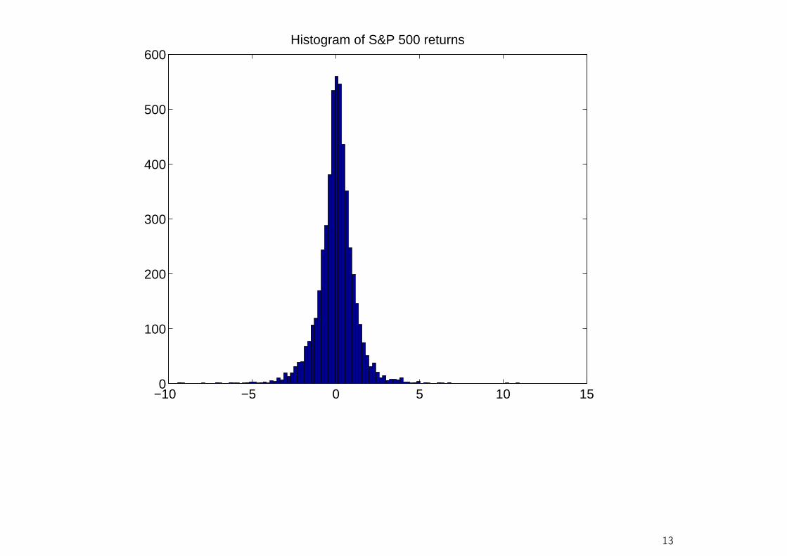
−10 −5 0 5 10 150
100
200
300
400
500
600Histogram of S&P 500 returns
13
−8 −6 −4 −2 0 2 4 6 80
0.1
0.2
0.3
0.4
0.5
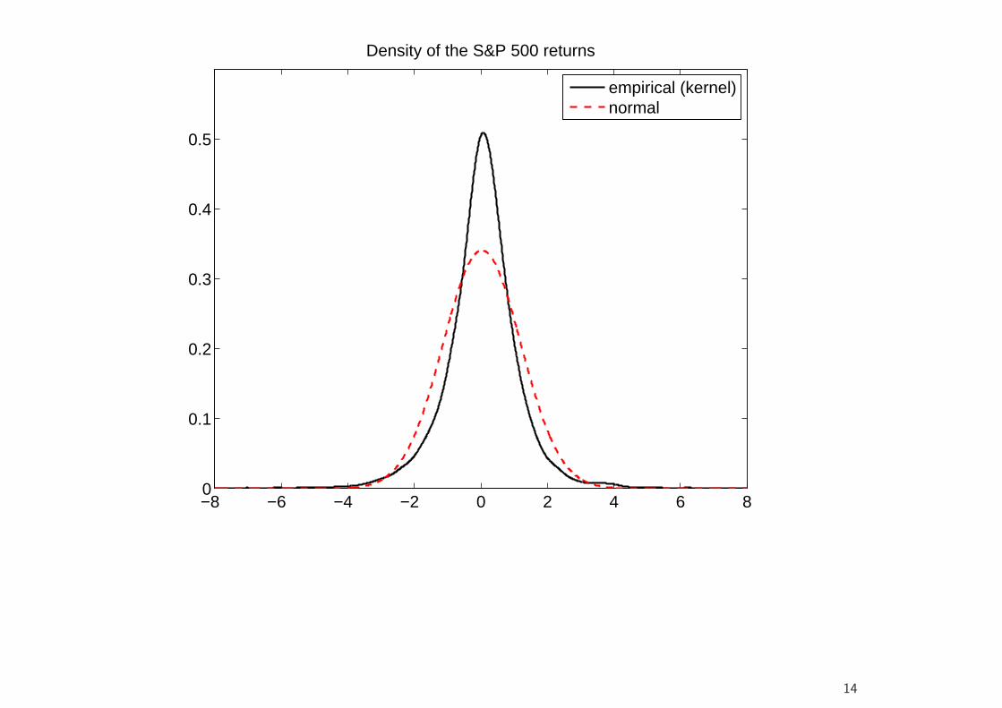
Density of the S&P 500 returns
empirical (kernel)normal
14
−8 −6 −4 −2 0 2 4 6 8−10
−9
−8
−7
−6
−5
−4
−3
−2
−1
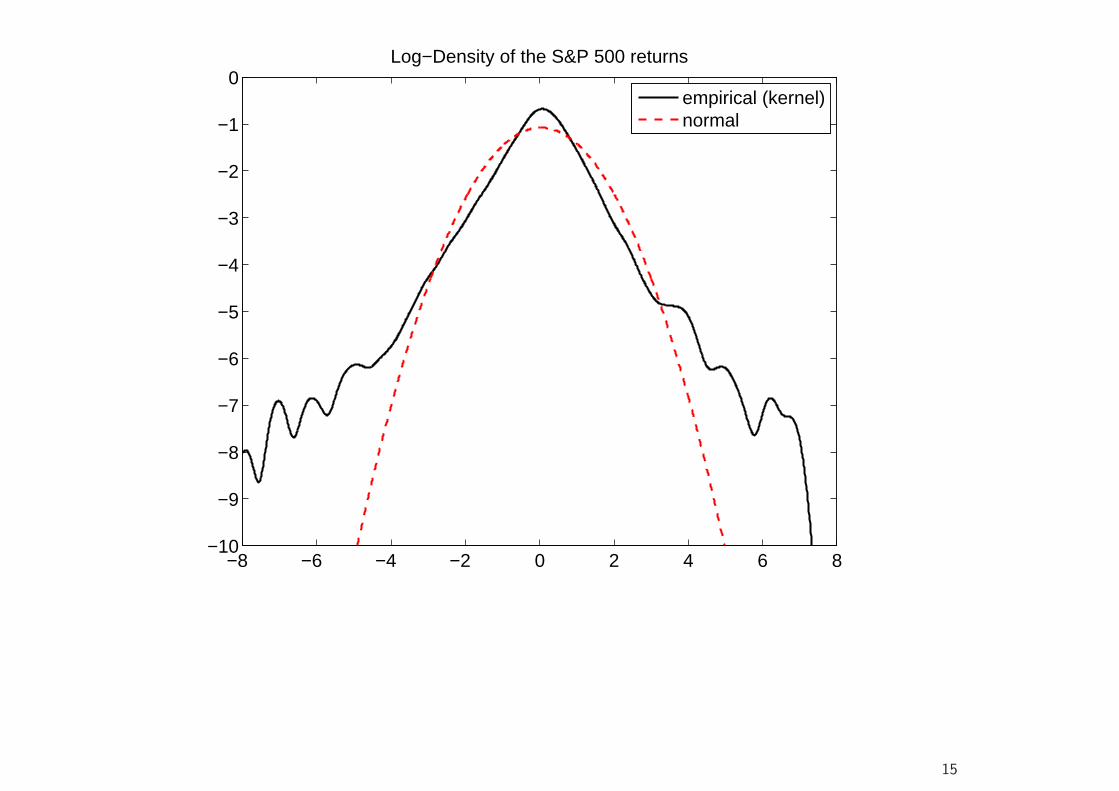
0Log−Density of the S&P 500 returns
empirical (kernel)normal
15

−10 −5 0 5 100
0.05
0.1
0.15
0.2
0.25
0.3
0.35
0.4Density of the DAX returns
empirical (kernel)normal
16

−8 −6 −4 −2 0 2 4 6 8−10
−9
−8
−7
−6
−5
−4
−3
−2
−1
0Log−Density of the DAX returns
empirical (kernel)normal
17

Basic Statistical Properties of Returns: ReturnDistribution
• Financial Returns at higher frequencies (higher than a month at least)are not normally distributed.
• In particular, they have much more probability mass in the center andthe tails than a normal distribution with the same variance.
• This implies, among other things, that the probability of large losses ismuch higher than under the Gaussian assumption.
• At lower frequencies, however, the central limit theorem appears tooperate, and the return distribution begins to closer resemble a Gaussianshape.
18

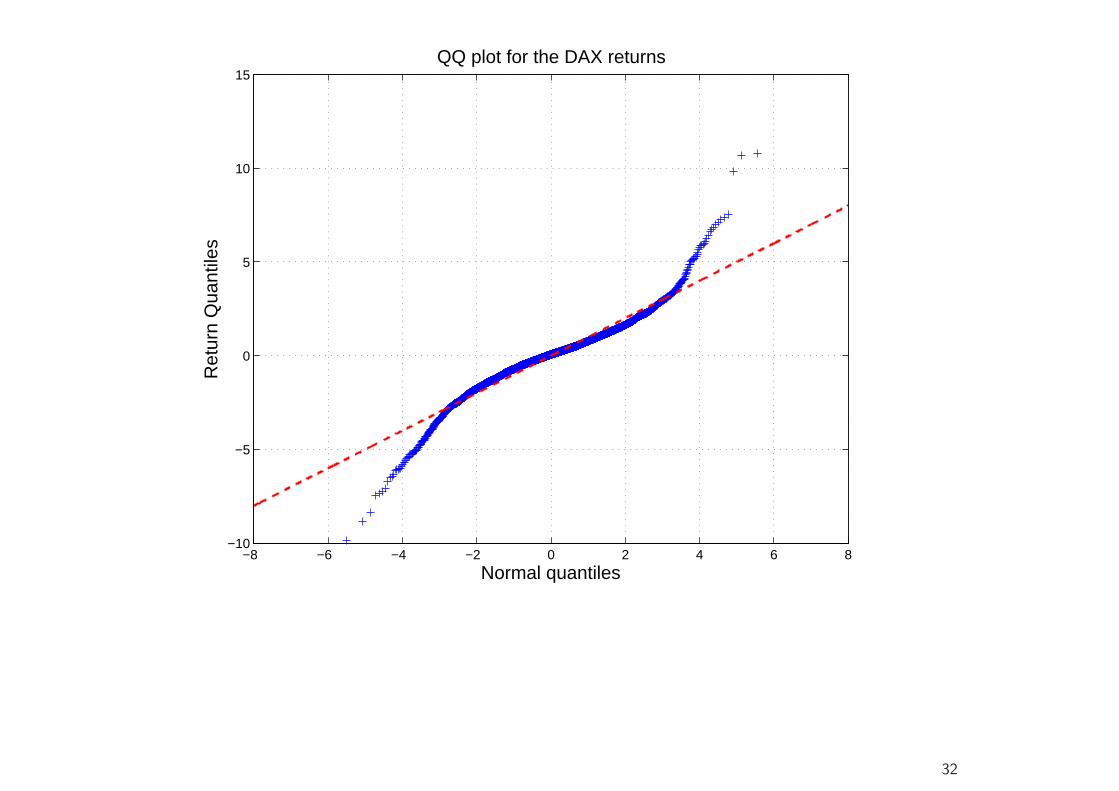
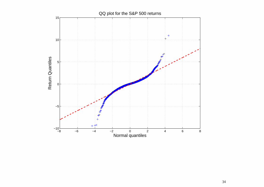
• A further simple device for detecting departures from normality (or anyother hypothesized distribution) are QQ plots.
• This is a scatter plot of the empirical quantiles (vertical axis) against thetheoretical quantiles (horizontal axis) of a given distribution (e.g., thenormal distribution).
• Excess kurtosis means that the probability of large negative or positivevalues is greater than under the corresponding normal density function.So the lower quantiles are smaller than the normal quantiles, and theupper quantiles are greater.
• Consequently, fat tails show up in QQ plots as deviations below an idealstraight line at the lower quantiles, and above the straight line at theupper quantiles.
19

−8 −6 −4 −2 0 2 4 6 8−10
−5
0
5
10
15QQ plot for the DAX returns
Normal quantiles
Ret
urn
Qua
ntile
s
20

−8 −6 −4 −2 0 2 4 6 8−10
−5
0
5
10
15QQ plot for the S&P 500 returns
Normal quantiles
Ret
urn
Qua
ntile
s
21

Kurtosis• A distribution with higher peaks and fatter tails (and, consequently, less
mass in the shoulders) than the normal is called “leptokurtic”.
• The standardized fourth moment is often calculated to measure thedegree of leptokurtosis, i.e.,
κ = kurtosis(r) =E(r − µ)4
σ4, (11)
where µ and σ2 are the mean and variance of r, respectively, and thesample analogue is
κ =T−1
∑Tt=1(rt − r)4
σ4, (12)
where r is the sample mean.
• For the normal distribution, κ = 3, and a distribution with κ > 3 is thenclassified as leptokurtic.
• The intuition is that the contribution of the rare and large returns in thetails is larger for the fourth moment than for the second (variance).
22

Kurtosis
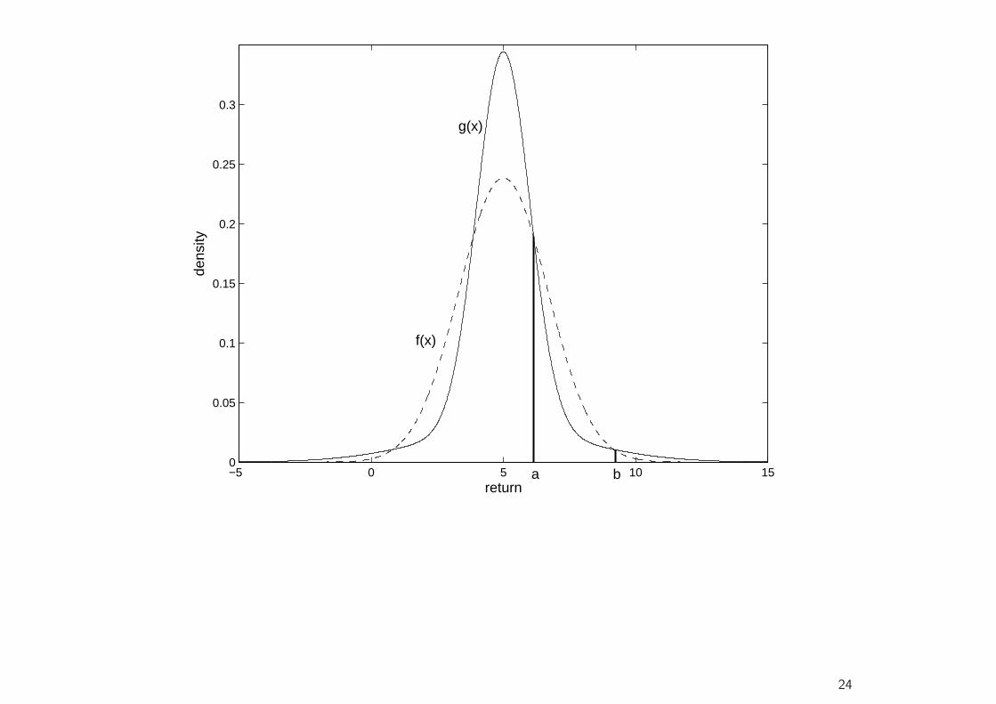
• Although this is the typical pattern of financial return data, it should bementioned that a high value of kurtosis does not always (in the sense ofa mathematical relationship) imply fatter tails and higher peaks than thenormal (or any other distribution).
• In fact, it can be shown that, if there are two densities f and g, eachbeing symmetrical with mean zero and common variance, and if thereare numbers a and b such that
g(x) < f(x) for a < |x| < b,
whereasg(x) > f(x) for |x| < a and |x| > b,
then the kurtosis measure κ (standardized fourth moment) is greater forg than for f .3
• The converse need not necessarily hold, however.3Finucan (1964): A Note on Kurtosis. Journal of the Royal Statistical Society 26, 111-112.
23
−5 0 5 10 150
0.05
0.1
0.15
0.2
0.25
0.3
return
dens
ity
a b
f(x)
g(x)
24
• The moment–based measures are still useful, however, and routinelycalculated in the literature.
• However, a nonparametric density estimate or QQ plot will in any casebe more informative.
25

Skewness
• Sometimes we also observe deviations from symmetry, although thesetend to be less pronounced and more difficult to detect.
• The moment–based skewness measure is
s = skewness(r) =E(r − µ)3
σ3, (13)
with sample counterpart
s =T−1
∑Tt=1(rt − µ)3
σ3. (14)
• For the normal, which is symmetric, s = 0.
26

Jarque–Bera test for normality
• Measures κ and s can be used to construct a test for normality.
• Under normality, sasy∼ Normal(0, 6/T ), and κ
asy∼ Normal(3, 24/T ), so
T s2/6asy∼ χ2(1), T (κ− 3)2/24
asy∼ χ2(1), (15)
and both are asymptotically independent, so
JB = T s2/6 + T (κ− 3)2/24asy∼ χ2(2), (16)
a χ2 distribution with two degrees of freedom.
• Note that we cannot easily use s as a basis for a test of symmetry.Although symmetric distributions always have s = 0, the asymptoticstandard error
√6/T is valid only under normality, and it is much larger
for fat–tailed symmetric distributions.
27

Alternative Distributions for Returns
• Mandelbrot (1963),4 in a famous study of cotton price changes, was oneof the first to point out the fat–tailed nature of return distributions.
• Mandelbrot suggested (nonnormal) α–stable (or stable Paretian)distributions as a generic model for asset returns, which may be viewedas a generalization of Osborne’s Gaussian model.
4B. Mandelbrot (1963). The Variation of Certain Speculative Prices. Journal of Business 36, 394-419.
28

Alternative Distributions for Returns: Discrete NormalMixtures
• A k–component (discrete) normal mixture distribution is described bythe density
f(x) =k∑
j=1
λjφ(x; µj, σ2j ), φ(x; µ, σ2) =
1√2πσ
exp{−(x− µ)2
2σ2
},
(17)λj > 0, j = 1, . . . , k, are the mixing weights, satisfying
∑j λj = 1, and
the µjs and σ2j s are the component means and variances respectively.
• Flexible with respect to skewness and kurtosis.
• A possible interpretation of the normal mixture is that returns arenormally distributed, but that return expectation and variance dependon the market regime, e.g., bull vs. bear markets.
29

• For the S&P 500 and the DAX, we find
Table 2: Normal mixture parameter estimatesλ1 µ1 σ2
1 λ2 µ2 σ22
S&P 500 0.801 0.071 0.518 0.199 −0.125 4.771
DAX 30 0.822 0.098 1.025 0.178 −0.285 7.580
• The basic mixture specification (17) can be generalized in variousdirections to provide a more satisfactory return model. For example,the mixing weights can be made time–varying, so that the regimes arepersistent or depend on exogenous or lagged endogenous variables.
30

−10 −8 −6 −4 −2 0 2 4 6 8 10−10
−5
0
5
10
15Normal mixture QQ plot for the DAX returns
Normal mixture quantiles
Ret
urn
Qua
ntile
s
31
−8 −6 −4 −2 0 2 4 6 8−10
−5
0
5
10
15QQ plot for the DAX returns
Normal quantiles
Ret
urn
Qua
ntile
s
32

−8 −6 −4 −2 0 2 4 6 8−10
−5
0
5
10
15Normal mixture QQ plot for the S&P 500 returns
Normal mixture quantiles
Ret
urn
Qua
ntile
s
33
−8 −6 −4 −2 0 2 4 6 8−10
−5
0
5
10
15QQ plot for the S&P 500 returns
Normal quantiles
Ret
urn
Qua
ntile
s
34

Alternative Distributions for Returns: Student’s t
• The standard Student’s t distribution with mean µ, scale σ and ν degreesof freedom has density
f(x) =Γ
(ν+12
)
Γ(ν/2)√
πνσ
{1 +
(x− µ)2
νσ2
}−(ν+1)/2
, ν > 0. (18)
• It can also be viewed as a (continuous) mixture of normals.
• The smaller ν, the fatter the tails, and normality is approached asν →∞.
• Generalizations that allow for skewness exist.
35

Alternative Distributions for Returns: GeneralizedExponential Distribution (GED)
• This has density
f(x) =2−(1/p+1)p
Γ(1/p)σexp
{−1
2
∣∣∣∣x− µ
σ
∣∣∣∣p}
, p > 0, (19)
where p measures the thickness of the tails.
• For p = 2, this nests the normal, and for p = 1 we get the Laplace(double exponential) distribution.
• Asymmetric extensions have been proposed.
36

Concentrating on the Tails: Extreme Value Theory• Often (e.g., when calculating risk measures such as Value–at–Risk) we
are not interested in the entire distribution of returns but only in theprobability of extreme events.
• We can then use extreme value theory to fully concentrate on the tailbehavior, without the need to model the central part of the distribution.
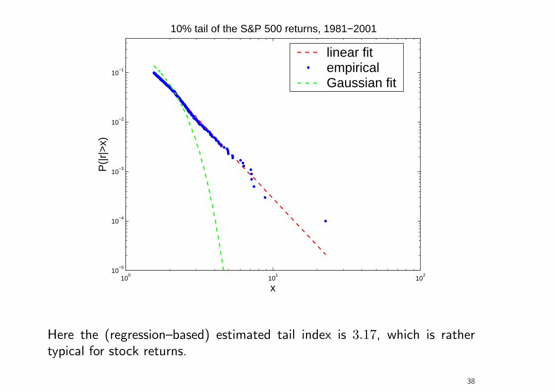
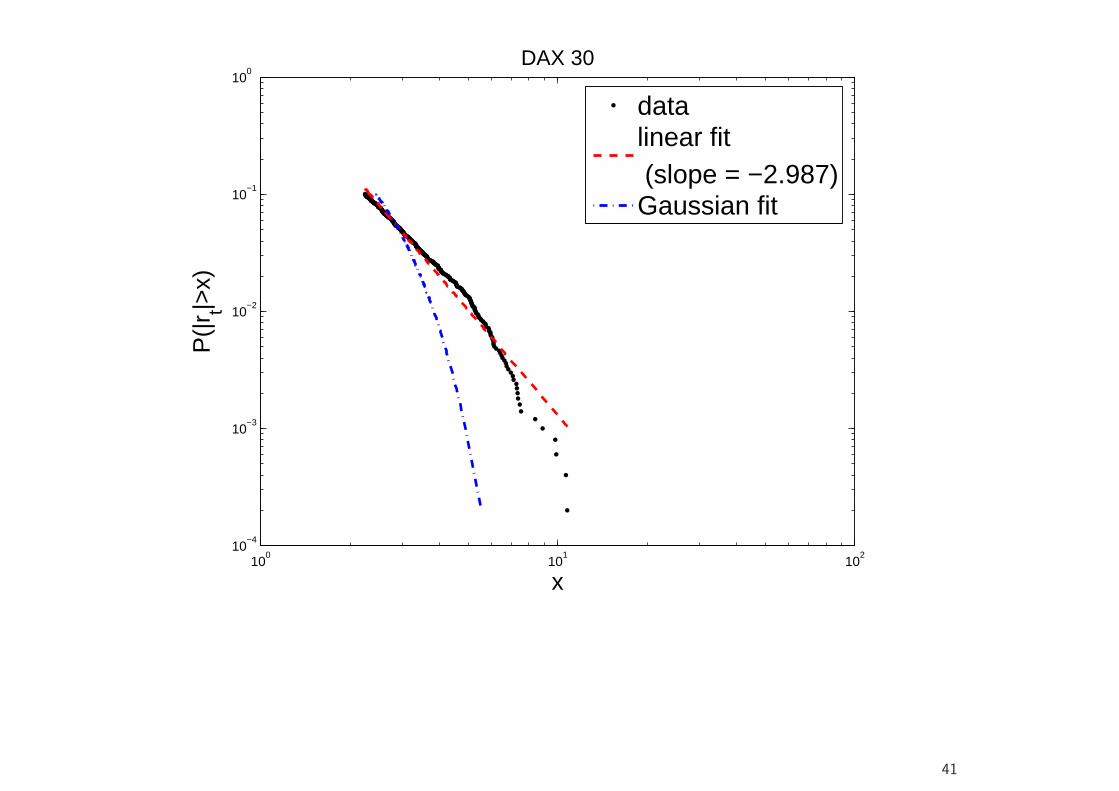
• It is often found that the tails of return distribution are well describedby a power law, i.e., for large x, with F being the distribution function(cdf),
1− F (x) = P (|r| > x) ≈ cx−α, (20)
where α is the tail exponent. In a log–log plot of the empiricalcomplementary cdf (1 − F (x)) against |r| (assuming symmetry), theobservations should approximately plot along a straight line (which canbe drawn using linear regression, log(1−F (x)) = log c−α log x, the slopeparameter is the tail exponent; but note that more efficient estimatorsexist for α).
• Several distributions are characterized by power law tails. For example,Student’s t has power tails with tail index ν.
37
100
101
102
10−5
10−4
10−3
10−2
10−1
10% tail of the S&P 500 returns, 1981−2001
x
P(|
r|>
x)
linear fitempiricalGaussian fit
Here the (regression–based) estimated tail index is 3.17, which is rathertypical for stock returns.
38

100.3
100.4
100.5
100.6
100.7
100.8
100.9
10−4
10−3
10−2
10−1
100
x
P(|
r t|>x)
FTSE 100
datalinear fit (slope = −2.983)Gaussian fit
39

100
101
102
10−4
10−3
10−2
10−1
100
x
P(|
r t|>x)
CAC 40
datalinear fit (slope = −3.105)Gaussian fit
40
100
101
102
10−4
10−3
10−2
10−1
100
x
P(|
r t|>x)
DAX 30
datalinear fit (slope = −2.987)Gaussian fit
41

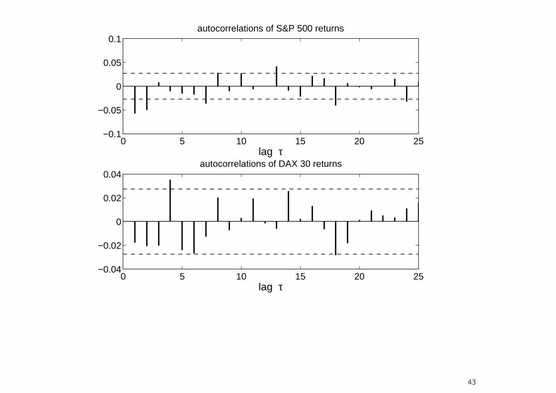
Temporal Properties of Returns
• Consider the sample autocorrelation function at lag τ ,
ρ(τ) =
T−τ∑t=1
(rt − r)(rt+τ − r)
T∑t=1
(rt − r)2, τ > 0, (21)
where
r =1T
T∑t=1
rt, (22)
and T is the sample size.
42
0 5 10 15 20 25−0.1
−0.05
0
0.05
0.1autocorrelations of S&P 500 returns
lag τ
0 5 10 15 20 25−0.04
−0.02
0
0.02
0.04autocorrelations of DAX 30 returns
lag τ
43

0 50 100 150 200 250−0.1
0
0.1
0.2
0.3
0.4autocorrelations of absolute (demeaned) S&P 500 returns
lag τ
0 50 100 150 200 250−0.1
0
0.1
0.2
0.3
0.4autocorrelations of squared (demeaned) S&P 500 returns
lag τ
44

0 50 100 150 200 250−0.05
0
0.05
0.1
0.15
0.2
0.25
0.3autocorrelations of absolute (demeaned) DAX 30 returns
lag τ
0 50 100 150 200 250−0.05
0
0.05
0.1
0.15
0.2
0.25
0.3autocorrelations of squared (demeaned) DAX 30 returns
lag τ
45

Temporal Properties of Returns
• Return series are characterized by volatility clustering, that is, “large[price] changes tend to be followed by large changes—of either sign—and small changes tend to be followed by small changes”.5
• Thus variance (and thus risk) appears to be persistent and predictable(in contrast to the direction of price changes).
• Several approaches for capturing time–varying volatility have beendeveloped, such as (G)ARCH, stochastic volatility, and regime–switchingmodels.
5B. Mandelbrot (1963). The Variation of Certain Speculative Prices. Journal of Business 36, 394-419.
46

Dependence Structure of Returns
• In basic portfolio theory, we are interested in the first two moments ofthe (portfolio) return distribution, i.e., mean and variance.
• In this framework, correlations between assets are of predominantinterest, because the strength of the correlations determines the degreeof risk (variance) reduction that can be achieved by efficient portfoliodiversification.
• Simple correlation estimates may be misleading, however, due toasymmetric dependence structures.
• This refers to the observation that, for example, stock returns are moredependent in bear markets (market downturns) than in bull markets.
• Therefore, diversification might fail when the benefits from diversificationare most urgently needed.
47

Dependence Structure of Returns
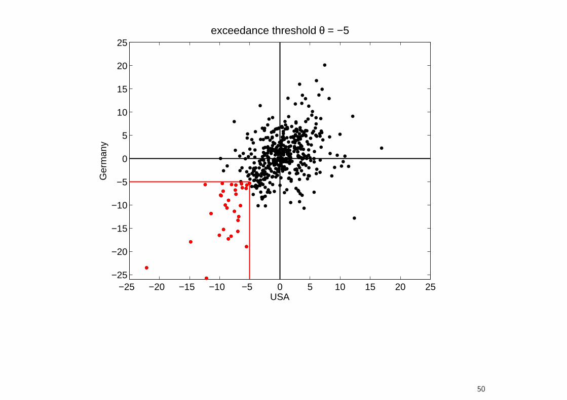
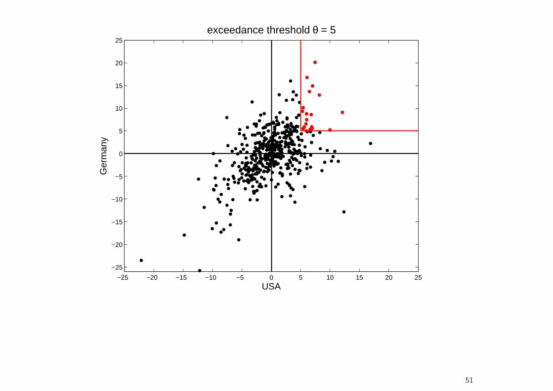
• A popular tool to describe this asymmetric dependence structure are theexceedance correlations of Longin and Solnik (2001).6
• For a given threshold θ, the exceedance correlation between (demeaned)returns r1 and r2 is given by
ρ(θ) =
{Corr(x, y|x > θ, y > θ) for θ ≥ 0Corr(x, y|x < θ, y < θ) for θ ≤ 0
(23)
• Let us consider monthly returns of MSCI stock market indices for the USand Germany from January 1970 to June 2008.
6Extreme Correlation of International Equity Markets. Journal of Finance 56, 649-676.
48

−25 −20 −15 −10 −5 0 5 10 15 20 25−25
−20
−15
−10
−5
0
5
10
15
20
25
USA
Ger
man
y
49
−25 −20 −15 −10 −5 0 5 10 15 20 25−25
−20
−15
−10
−5
0
5
10
15
20
25
USA
Ger
man
y
exceedance threshold θ = −5
50
−25 −20 −15 −10 −5 0 5 10 15 20 25
−25
−20
−15
−10
−5
0
5
10
15
20
25
USA
Ger
man
y
exceedance threshold θ = 5
51
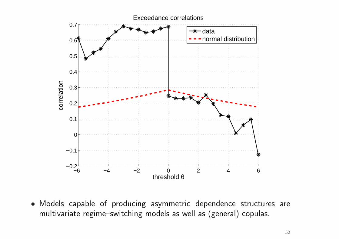
−6 −4 −2 0 2 4 6−0.2
−0.1
0
0.1
0.2
0.3
0.4
0.5
0.6
0.7Exceedance correlations
threshold θ
corr
elat
ion
datanormal distribution
• Models capable of producing asymmetric dependence structures aremultivariate regime–switching models as well as (general) copulas.
52