UseR 2017Dose-response analysis in toxicologyand epidemiology: considering dose

both as qualitative factor andquantitative covariate- using R

Ludwig A. Hothornretired Leibniz University Hannover, Germany

Joint work with F. Schaarschmidt and Ch. Ritz

July 6, 2017

1 / 55

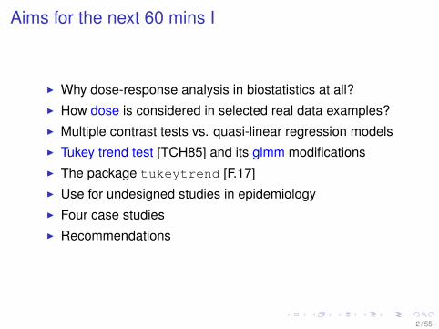
Aims for the next 60 mins I

I Why dose-response analysis in biostatistics at all?I How dose is considered in selected real data examples?I Multiple contrast tests vs. quasi-linear regression modelsI Tukey trend test [TCH85] and its glmm modificationsI The package tukeytrend [F.17]I Use for undesigned studies in epidemiologyI Four case studiesI Recommendations

2 / 55

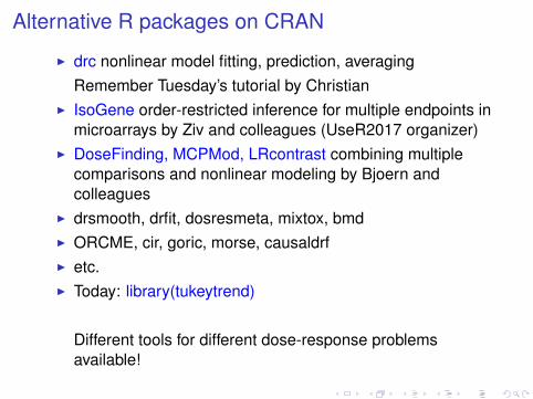
Alternative R packages on CRAN

I drc nonlinear model fitting, prediction, averagingRemember Tuesday’s tutorial by Christian

I IsoGene order-restricted inference for multiple endpoints inmicroarrays by Ziv and colleagues (UseR2017 organizer)

I DoseFinding, MCPMod, LRcontrast combining multiplecomparisons and nonlinear modeling by Bjoern andcolleagues

I drsmooth, drfit, dosresmeta, mixtox, bmdI ORCME, cir, goric, morse, causaldrfI etc.I Today: library(tukeytrend)

Different tools for different dose-response problemsavailable!

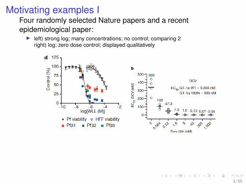
Motivating examples IFour randomly selected Nature papers and a recentepidemiological paper:

I left) strong log; many concentrations; no control; comparing 2right) log; zero dose control; displayed qualitatively

3 / 55

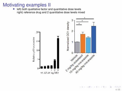
Motivating examples III left) both qualitative factor and quantitative dose levels

right) reference drug and 2 quantitative dose levels mixed

4 / 55

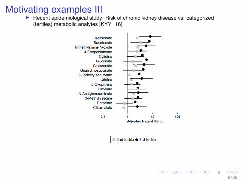
Motivating examples IIII Recent epidemiological study: Risk of chronic kidney disease vs. categorized

(tertiles) metabolic analytes [KYY+16]

5 / 55

Motivating examples IV

I Quantitative covariable and/or qualitative factor (even aftercategorization!)

I Assuming log transformation quite commonI Why log-transformation, and how log(C=0)?I Both regression model I, i.e. grouped dose levels and

model II: randomly chosen dose levelsI Multiple endpoints common, recently high-dimI ...

6 / 55

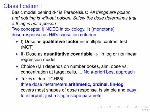
Classification IBasic model behind d-r is Paracelsius: All things are poisonand nothing is without poison. Solely the dose determines thata thing is not a poisonTwo concepts: i) NOEC in toxicology, ii) (monotone)dose-response as Hill’s causation criterion

I I) Dose as qualitative factor⇒ multiple contrast test(MCT)

I II) Dose as quantitative covariable⇒ lin-log or nonlinearregression model

I Choice (I,II) depends on number doses, aim, dose vs.concentration at target cells, ... No a-priori best approach

I Tukey’s idea [TCH85]:three dose metameters arithmetic, ordinal, lin-logcovers most shapes of dose response, is simple and easyto interpret: just a single slope parameter

7 / 55

Classification II

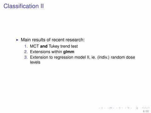
I Main results of recent research:1. MCT and Tukey trend test2. Extensions within glmm3. Extension to regression model II, ie. (indiv.) random dose

levels

8 / 55

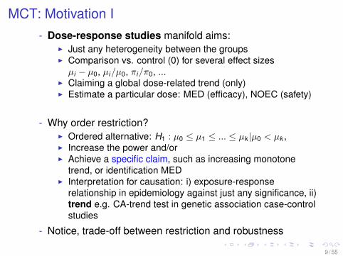
MCT: Motivation I- Dose-response studies manifold aims:

I Just any heterogeneity between the groupsI Comparison vs. control (0) for several effect sizesµi − µ0, µi/µ0, πi/π0, ...

I Claiming a global dose-related trend (only)I Estimate a particular dose: MED (efficacy), NOEC (safety)

- Why order restriction?I Ordered alternative: H1 : µ0 ≤ µ1 ≤ ... ≤ µk |µ0 < µk ,I Increase the power and/orI Achieve a specific claim, such as increasing monotone

trend, or identification MEDI Interpretation for causation: i) exposure-response

relationship in epidemiology against just any significance, ii)trend e.g. CA-trend test in genetic association case-controlstudies

- Notice, trade-off between restriction and robustness

9 / 55

Order restricted tests and related simultaneousconfidence intervals I

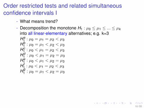
- What means trend?- Decomposition the monotone H1 : µ0 ≤ µ1 ≤ ... ≤ µk

into all linear-elementary alternatives; e.g. k=3Ha

1 : µ0 = µ1 = µ2 < µ3Hb

1 : µ0 = µ1 < µ2 < µ3Hc

1 : µ0 < µ1 = µ2 < µ3Hd

1 : µ0 < µ1 = µ2 = µ3He

1 : µ0 < µ1 < µ2 = µ3H f

1 : µ0 < µ1 = µ2 < µ3Hg

1 : µ0 = µ1 < µ2 = µ3

10 / 55

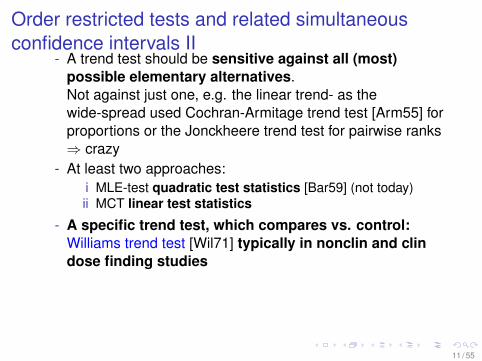
Order restricted tests and related simultaneousconfidence intervals II

- A trend test should be sensitive against all (most)possible elementary alternatives.Not against just one, e.g. the linear trend- as thewide-spread used Cochran-Armitage trend test [Arm55] forproportions or the Jonckheere trend test for pairwise ranks⇒ crazy

- At least two approaches:i MLE-test quadratic test statistics [Bar59] (not today)ii MCT linear test statistics

- A specific trend test, which compares vs. control:Williams trend test [Wil71] typically in nonclin and clindose finding studies

11 / 55

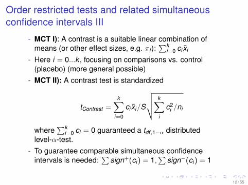
Order restricted tests and related simultaneousconfidence intervals III

- MCT I): A contrast is a suitable linear combination ofmeans (or other effect sizes, e.g. πi ):

∑ki=0 ci xi

- Here i = 0...k , focusing on comparisons vs. control(placebo) (more general possible)

- MCT II): A contrast test is standardized

tContrast =k∑

i=0

ci xi/S

√√√√ k∑i

c2i /ni

where∑k

i=0 ci = 0 guaranteed a tdf ,1−α distributedlevel-α-test.

- To guarantee comparable simultaneous confidenceintervals is needed:

∑sign+(ci) = 1,

∑sign−(ci) = 1

12 / 55

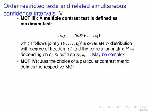
Order restricted tests and related simultaneousconfidence intervals IV

- MCT III): A multiple contrast test is defined asmaximum test:

tMCT = max(t1, ..., tq)

which follows jointly (t1, . . . , tq)′ a q-variate t- distributionwith degree of freedom df and the correlation matrix R ⇒depending on ci ,ni but also si , ρi , ... May be complex

- MCT IV): Just the choice of a particular contrast matrixdefines the respective MCT

13 / 55

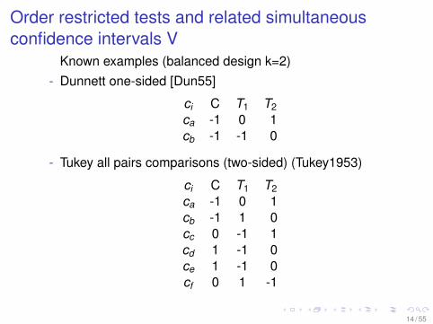
Order restricted tests and related simultaneousconfidence intervals V

Known examples (balanced design k=2)- Dunnett one-sided [Dun55]

ci C T1 T2ca -1 0 1cb -1 -1 0

- Tukey all pairs comparisons (two-sided) (Tukey1953)

ci C T1 T2ca -1 0 1cb -1 1 0cc 0 -1 1cd 1 -1 0ce 1 -1 0cf 0 1 -1

14 / 55

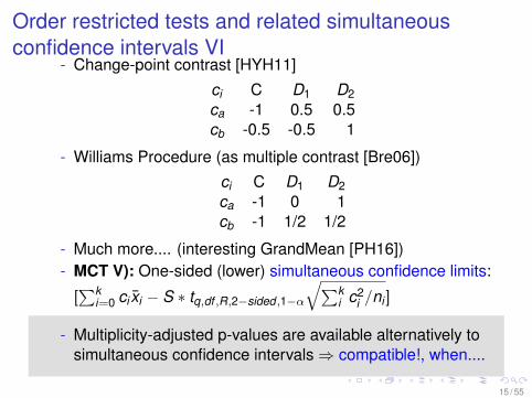
Order restricted tests and related simultaneousconfidence intervals VI

- Change-point contrast [HYH11]

ci C D1 D2ca -1 0.5 0.5cb -0.5 -0.5 1

- Williams Procedure (as multiple contrast [Bre06])

ci C D1 D2ca -1 0 1cb -1 1/2 1/2

- Much more.... (interesting GrandMean [PH16])- MCT V): One-sided (lower) simultaneous confidence limits:

[∑k

i=0 ci xi − S ∗ tq,df ,R,2−sided ,1−α

√∑ki c2

i /ni ]

- Multiplicity-adjusted p-values are available alternatively tosimultaneous confidence intervals⇒ compatible!, when....

15 / 55

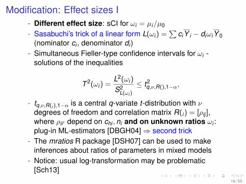
Modification: Effect sizes I- Different effect size: sCI for ωi = µi/µ0

- Sasabuchi’s trick of a linear form L(ωi) =∑

ciY i − diωiY 0(nominator ci , denominator di )

- Simultaneous Fieller-type confidence intervals for ωi -solutions of the inequalities

T 2(ωi) =L2(ωi)

S2L(ωi )

≤ t2q,ν,R(),1−α,

- tq,ν,R(i ),1−α is a central q-variate t-distribution with νdegrees of freedom and correlation matrix R(i) = [ρij ],where ρii ′ depend on chi ,ni and on unknown ratios ωi :plug-in ML-estimators [DBGH04]⇒ second trick

- The mratios R package [DSH07] can be used to makeinferences about ratios of parameters in mixed models

- Notice: usual log-transformation may be problematic[Sch13]

16 / 55

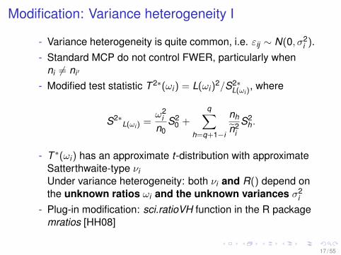
Modification: Variance heterogeneity I

- Variance heterogeneity is quite common, i.e. εij ∼ N(0, σ2i ).

- Standard MCP do not control FWER, particularly whenni 6= ni ′

- Modified test statistic T 2∗(ωi) = L(ωi)2/S2∗

L(ωi ), where

S2∗L(ωi ) =

ω2i

n0S2

0 +

q∑h=q+1−i

nh

n2i

S2h .

- T ∗(ωi) has an approximate t-distribution with approximateSatterthwaite-type νiUnder variance heterogeneity: both νi and R() depend onthe unknown ratios ωi and the unknown variances σ2

i

- Plug-in modification: sci.ratioVH function in the R packagemratios [HH08]

17 / 55

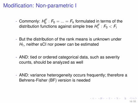
Modification: Non-parametric I

- Commonly: HF0 : F0 = ... = Fk formulated in terms of the

distribution functions against simple tree HF1 : F0 < Fi

- But the distribution of the rank means is unknown underH1, neither sCI nor power can be estimated

- AND: tied or ordered categorical data, such as severitycounts, should be analyzed as well

- AND: variance heterogeneity occurs frequently; therefore aBehrens-Fisher (BF) version is needed

18 / 55

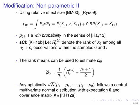
Modification: Non-parametric II- Using relative effect size [BM00], [Ryu09]:

p01 =

∫F0dF1 = P(X01 < X11) + 0.5P(X01 = X11).

- p01 is a win probability in the sense of [Hay13]

- sCI: [KH12b] Let R(0l)lj denote the rank of Xlj among all

n0 + nl observations within the samples 0 and l

- The rank means can be used to estimate p0l

p0l =1n0

(R

(0l)l· −

nl + 12

)- Asymptotically

√N(p1 − p1, . . . , pq − pq)′ follows a central

multivariate normal distribution with expectation 0 andcovariance matrix VN [KH12a]

19 / 55

Modification: Non-parametric III

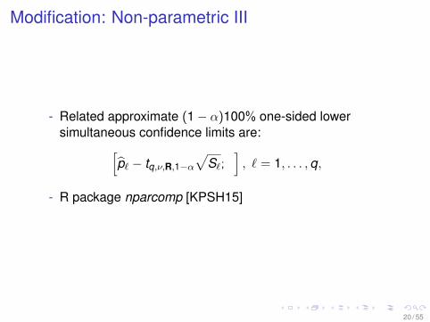
- Related approximate (1− α)100% one-sided lowersimultaneous confidence limits are:[

p` − tq,ν,R,1−α√

S`;], ` = 1, . . . ,q,

- R package nparcomp [KPSH15]

20 / 55

Modification: Proportions I

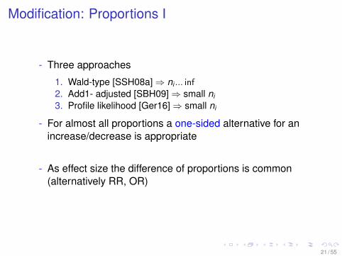
- Three approaches

1. Wald-type [SSH08a]⇒ ni ... inf2. Add1- adjusted [SBH09]⇒ small ni

3. Profile likelihood [Ger16]⇒ small ni

- For almost all proportions a one-sided alternative for anincrease/decrease is appropriate

- As effect size the difference of proportions is common(alternatively RR, OR)

21 / 55

Modification: Proportions II

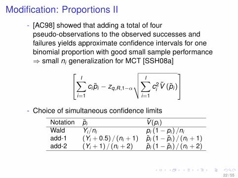
- [AC98] showed that adding a total of fourpseudo-observations to the observed successes andfailures yields approximate confidence intervals for onebinomial proportion with good small sample performance⇒ small ni generalization for MCT [SSH08a] I∑

i=1

ci pi − zq,R,1−α

√√√√ I∑i=1

c2i V (pi)

- Choice of simultaneous confidence limits

Notation pi V (pi )Wald Yi/ni pi (1− pi ) /niadd-1 (Yi + 0.5) / (ni + 1) pi (1− pi ) / (ni + 1)add-2 (Yi + 1) / (ni + 2) pi (1− pi ) / (ni + 2)

22 / 55

Modification: Further Williams-type sCI I

- Comparing survival functions: i) Cox proport. hazardsmodel or ii) the frailty Cox model to allow a joint analysisover sex and strains [HH12]

- Multiple endpoints: UIT(UIT) [HH13]: R package SimComp

- Poly-k estimates [SSH08b]

- ....

23 / 55

Tukey’s trend test- Intro I

I Up to now: dose as a qualitative factor

I Now: considering dose asquantitative covariate

24 / 55

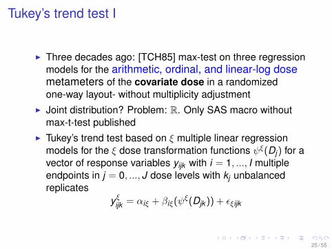
Tukey’s trend test I

I Three decades ago: [TCH85] max-test on three regressionmodels for the arithmetic, ordinal, and linear-log dosemetameters of the covariate dose in a randomizedone-way layout- without multiplicity adjustment

I Joint distribution? Problem: R. Only SAS macro withoutmax-t-test published

I Tukey’s trend test based on ξ multiple linear regressionmodels for the ξ dose transformation functions ψξ(Dj) for avector of response variables yijk with i = 1, ..., I multipleendpoints in j = 0, ..., J dose levels with kj unbalancedreplicates

yξijk = αiξ + βiξ(ψξ(Djk )) + εξijk

25 / 55

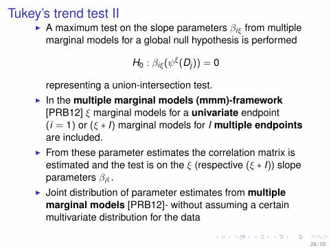
Tukey’s trend test III A maximum test on the slope parameters βiξ from multiple

marginal models for a global null hypothesis is performed

H0 : βiξ(ψξ(Dj)) = 0

representing a union-intersection test.I In the multiple marginal models (mmm)-framework

[PRB12] ξ marginal models for a univariate endpoint(i = 1) or (ξ ∗ I) marginal models for I multiple endpointsare included.

I From these parameter estimates the correlation matrix isestimated and the test is on the ξ (respective (ξ ∗ I)) slopeparameters βiξ .

I Joint distribution of parameter estimates from multiplemarginal models [PRB12]- without assuming a certainmultivariate distribution for the data

26 / 55

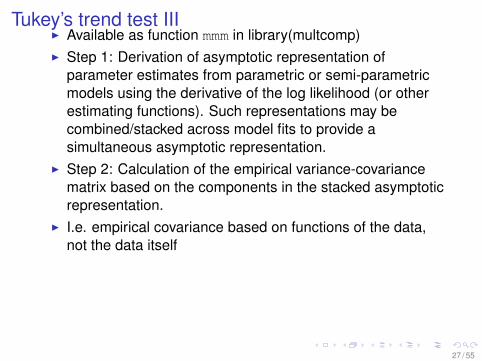
Tukey’s trend test IIII Available as function mmm in library(multcomp)I Step 1: Derivation of asymptotic representation of

parameter estimates from parametric or semi-parametricmodels using the derivative of the log likelihood (or otherestimating functions). Such representations may becombined/stacked across model fits to provide asimultaneous asymptotic representation.

I Step 2: Calculation of the empirical variance-covariancematrix based on the components in the stacked asymptoticrepresentation.

I I.e. empirical covariance based on functions of the data,not the data itself

27 / 55

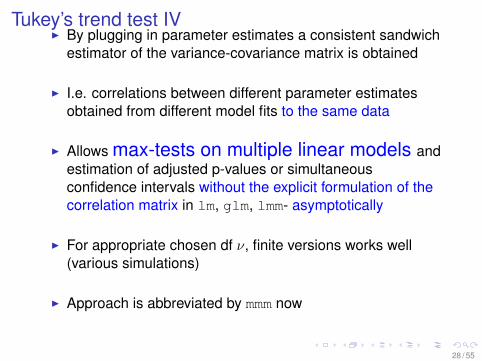
Tukey’s trend test IVI By plugging in parameter estimates a consistent sandwich

estimator of the variance-covariance matrix is obtained

I I.e. correlations between different parameter estimatesobtained from different model fits to the same data

I Allows max-tests on multiple linear models andestimation of adjusted p-values or simultaneousconfidence intervals without the explicit formulation of thecorrelation matrix in lm, glm, lmm- asymptotically

I For appropriate chosen df ν, finite versions works well(various simulations)

I Approach is abbreviated by mmm now

28 / 55

Tukey’s trend test V

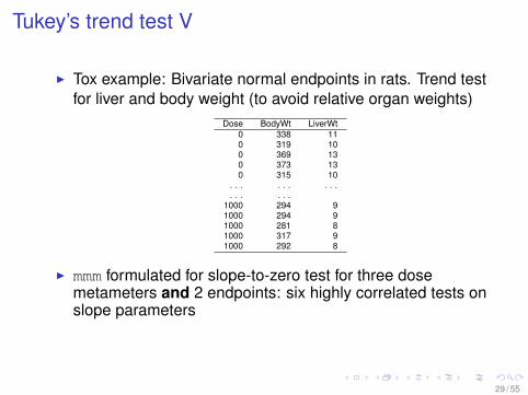
I Tox example: Bivariate normal endpoints in rats. Trend testfor liver and body weight (to avoid relative organ weights)

Dose BodyWt LiverWt0 338 110 319 100 369 130 373 130 315 10

. . . . . . . . .

. . . . . .1000 294 91000 294 91000 281 81000 317 91000 292 8

I mmm formulated for slope-to-zero test for three dosemetameters and 2 endpoints: six highly correlated tests onslope parameters

29 / 55

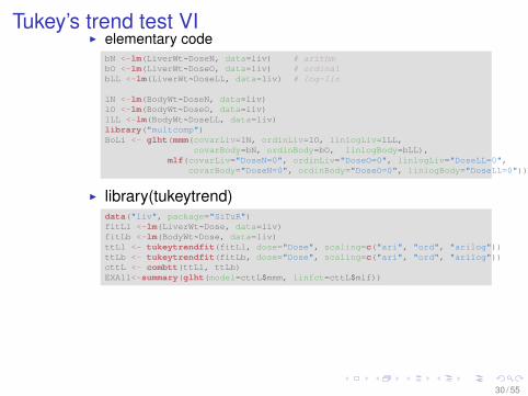
Tukey’s trend test VII elementary code

bN <-lm(LiverWt~DoseN, data=liv) # arithmbO <-lm(LiverWt~DoseO, data=liv) # ordinalbLL <-lm(LiverWt~DoseLL, data=liv) # log-lin

lN <-lm(BodyWt~DoseN, data=liv)lO <-lm(BodyWt~DoseO, data=liv)lLL <-lm(BodyWt~DoseLL, data=liv)library("multcomp")BoLi <- glht(mmm(covarLiv=lN, ordinLiv=lO, linlogLiv=lLL,

covarBody=bN, ordinBody=bO, linlogBody=bLL),mlf(covarLiv="DoseN=0", ordinLiv="DoseO=0", linlogLiv="DoseLL=0",

covarBody="DoseN=0", ordinBody="DoseO=0", linlogBody="DoseLL=0"))

I library(tukeytrend)data("liv", package="SiTuR")fitLl <-lm(LiverWt~Dose, data=liv)fitLb <-lm(BodyWt~Dose, data=liv)ttLl <- tukeytrendfit(fitLl, dose="Dose", scaling=c("ari", "ord", "arilog"))ttLb <- tukeytrendfit(fitLb, dose="Dose", scaling=c("ari", "ord", "arilog"))cttL <- combtt(ttLl, ttLb)EXA11<-summary(glht(model=cttL$mmm, linfct=cttL$mlf))

30 / 55

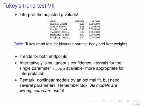
Tukey’s trend test VIII Interpret the adjusted p-values!

Model Test stats p-valuecovarLiv: DoseN -5.38 0.0000001ordinLiv: DoseO -3.98 0.0001253linlogLiv: DoseLL -3.98 0.0002106covarBody: DoseN -6.04 0.0000000ordinBody: DoseO -5.17 0.0000003linlogBody: DoseLL -5.17 0.0000004

Table: Tukey trend test for bivariate normal: body and liver weights

I Trends for both endpointsI Alternatively, simultaneous confidence intervals for the

single parameter slope available- more appropriate forinterpretation!

I Remark: nonlinear models try an optimal fit, but needseveral parameters. Remember Box: All models arewrong, some are useful

31 / 55

Trend test using both a covariate and a factor II To assume dose as a qualitative factor or a quantitative

covariate result in quite different- disjoint- approaches:trend tests or non-linear models

I Common perception: trend test and (non)linear models arecompletely separate approaches -not necessarily →

I Extension of the Tukey trend test:i) three regression models for the arithmetic, ordinal, andlogarithmic-linear dose metameters [TCH85] AND ii)Williams multiple contrast

32 / 55

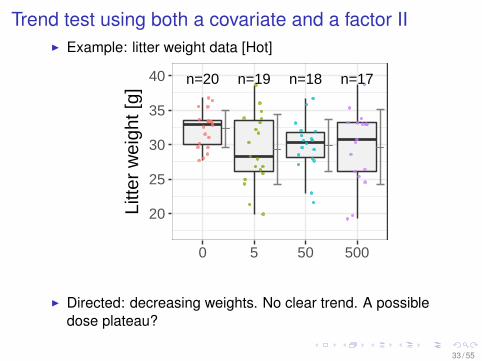
Trend test using both a covariate and a factor III Example: litter weight data [Hot]

n=20 n=19 n=18 n=17

20

25

30

35

40

0 5 50 500

Litte

r w

eigh

t [g]

I Directed: decreasing weights. No clear trend. A possibledose plateau?

33 / 55

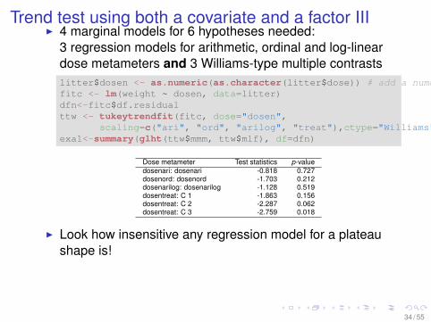
Trend test using both a covariate and a factor IIII 4 marginal models for 6 hypotheses needed:

3 regression models for arithmetic, ordinal and log-lineardose metameters and 3 Williams-type multiple contrastslitter$dosen <- as.numeric(as.character(litter$dose)) # add a numeric dose variablefitc <- lm(weight ~ dosen, data=litter)dfn<-fitc$df.residualttw <- tukeytrendfit(fitc, dose="dosen",

scaling=c("ari", "ord", "arilog", "treat"),ctype="Williams")exa1<-summary(glht(ttw$mmm, ttw$mlf), df=dfn)

Dose metameter Test statistics p-valuedosenari: dosenari -0.818 0.727dosenord: dosenord -1.703 0.212dosenarilog: dosenarilog -1.128 0.519dosentreat: C 1 -1.863 0.156dosentreat: C 2 -2.287 0.062dosentreat: C 3 -2.759 0.018

I Look how insensitive any regression model for a plateaushape is!

34 / 55

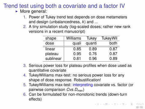
Trend test using both a covariate and a factor IVI More general:

1. Power of Tukey trend test depends on dose metametersand design (unbalancedness, k ) and ...

2. A tiny simulation study (log-scaled doses; rather new rankversions in a recent manuscript)

shape Williams Tukey TukeyWildose quali quanti bothlinear 0.85 0.89 0.87plateau 0.95 0.76 0.87sublinear 0.81 0.96 0.89

3. Serious power loss for plateau profiles when dose used asquantitative covariate

4. TukeyWilliams max-test: no serious power loss for anyshape of dose response. Robustification!

5. TukeyWilliams max-test: interpreting covariate vs. factor (orpairwise comparison Cvs.Dmax )

6. Can be formulated for non-monotonic trends (down-turneffects)

35 / 55

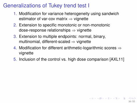
Generalizations of Tukey trend test I1. Modification for variance heterogeneity using sandwich

estimator of var-cov matrix⇒ vignette2. Extension to specific monotonic or non-monotonic

dose-response relationships⇒ vignette3. Extension to multiple endpoints: normal, binary,

multinomial, different-scaled⇒ vignette4. Modification for different arithmetic-logarithmic scores⇒

vignette5. Inclusion of the control vs. high dose comparison [AXL11]

36 / 55

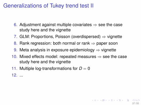
Generalizations of Tukey trend test II

6. Adjustment against multiple covariates⇒ see the casestudy here and the vignette

7. GLM: Proportions, Poisson (overdispersed)⇒ vignette

8. Rank regression: both normal or rank⇒ paper soon

9. Meta analysis in exposure epidemiology⇒ vignette

10. Mixed effects model: repeated measures⇒ see the casestudy here and the vignette

11. Multiple log-transformations for D = 0

12. ...

37 / 55

Mixed effects model: technical replicates I

I The analysis of designs with technical replicates isperformed often naive. But mixed model(s) are available

I Nonclin example: Per-litter data as natural replicatesI The jittered boxplots show rather different litter sizes

38 / 55

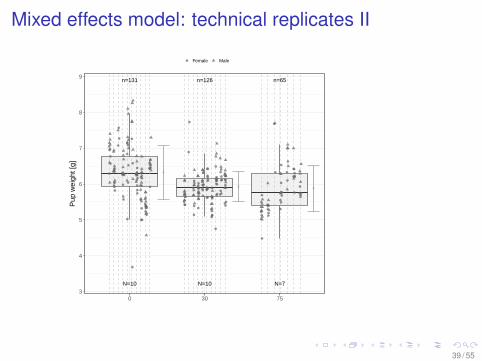
Mixed effects model: technical replicates II

n=131 n=126 n=65

N=10 N=10 N=73

4

5

6

7

8

9

0 30 75

Pup

wei

ght [

g]

Female Male

39 / 55

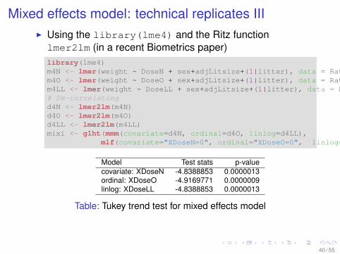
Mixed effects model: technical replicates IIII Using the library(lme4) and the Ritz functionlmer2lm (in a recent Biometrics paper)library(lme4)m4N <- lmer(weight ~ DoseN + sex+adjLitsize+(1|litter), data = Ratpup)m4O <- lmer(weight ~ DoseO + sex+adjLitsize+(1|litter), data = Ratpup)m4LL <- lmer(weight ~ DoseLL + sex+adjLitsize+(1|litter), data = Ratpup)# De-correlatingd4N <- lmer2lm(m4N)d4O <- lmer2lm(m4O)d4LL <- lmer2lm(m4LL)mixi <- glht(mmm(covariate=d4N, ordinal=d4O, linlog=d4LL),

mlf(covariate="XDoseN=0", ordinal="XDoseO=0", linlog="XDoseLL=0"))

Model Test stats p-valuecovariate: XDoseN -4.8388853 0.0000013ordinal: XDoseO -4.9169771 0.0000009linlog: XDoseLL -4.8388853 0.0000013

Table: Tukey trend test for mixed effects model

40 / 55

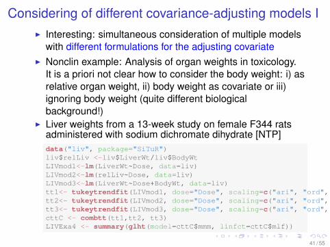
Considering of different covariance-adjusting models II Interesting: simultaneous consideration of multiple models

with different formulations for the adjusting covariateI Nonclin example: Analysis of organ weights in toxicology.

It is a priori not clear how to consider the body weight: i) asrelative organ weight, ii) body weight as covariate or iii)ignoring body weight (quite different biologicalbackground!)

I Liver weights from a 13-week study on female F344 ratsadministered with sodium dichromate dihydrate [NTP]data("liv", package="SiTuR")liv$relLiv <-liv$LiverWt/liv$BodyWtLIVmod1<-lm(LiverWt~Dose, data=liv)LIVmod2<-lm(relLiv~Dose, data=liv)LIVmod3<-lm(LiverWt~Dose+BodyWt, data=liv)tt1<- tukeytrendfit(LIVmod1, dose="Dose", scaling=c("ari", "ord", "arilog"))tt2<- tukeytrendfit(LIVmod2, dose="Dose", scaling=c("ari", "ord", "arilog"))tt3<- tukeytrendfit(LIVmod3, dose="Dose", scaling=c("ari", "ord", "arilog"))cttC <- combtt(tt1,tt2, tt3)LIVExa4 <- summary(glht(model=cttC$mmm, linfct=cttC$mlf))

41 / 55

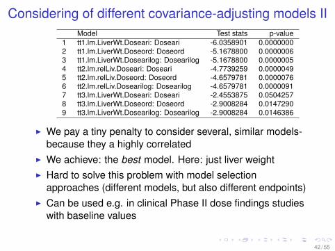
Considering of different covariance-adjusting models IIModel Test stats p-value

1 tt1.lm.LiverWt.Doseari: Doseari -6.0358901 0.00000002 tt1.lm.LiverWt.Doseord: Doseord -5.1678800 0.00000063 tt1.lm.LiverWt.Dosearilog: Dosearilog -5.1678800 0.00000054 tt2.lm.relLiv.Doseari: Doseari -4.7739259 0.00000495 tt2.lm.relLiv.Doseord: Doseord -4.6579781 0.00000766 tt2.lm.relLiv.Dosearilog: Dosearilog -4.6579781 0.00000917 tt3.lm.LiverWt.Doseari: Doseari -2.4553875 0.05042578 tt3.lm.LiverWt.Doseord: Doseord -2.9008284 0.01472909 tt3.lm.LiverWt.Dosearilog: Dosearilog -2.9008284 0.0146386

I We pay a tiny penalty to consider several, similar models-because they a highly correlated

I We achieve: the best model. Here: just liver weightI Hard to solve this problem with model selection

approaches (different models, but also different endpoints)I Can be used e.g. in clinical Phase II dose findings studies

with baseline values

42 / 55

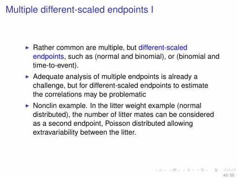
Multiple different-scaled endpoints I

I Rather common are multiple, but different-scaledendpoints, such as (normal and binomial), or (binomial andtime-to-event).

I Adequate analysis of multiple endpoints is already achallenge, but for different-scaled endpoints to estimatethe correlations may be problematic

I Nonclin example. In the litter weight example (normaldistributed), the number of litter mates can be consideredas a second endpoint, Poisson distributed allowingextravariability between the litter.

43 / 55

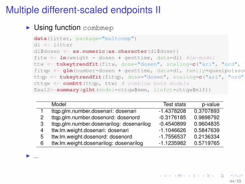
Multiple different-scaled endpoints II

I Using function combmep

data(litter, package="multcomp")dl <- litterdl$dosen <- as.numeric(as.character(dl$dose))fitw <- lm(weight ~ dosen + gesttime, data=dl) #lm-modelttw <- tukeytrendfit(fitw, dose="dosen", scaling=c("ari", "ord", "arilog"))fitqp <- glm(number~dosen + gesttime, data=dl, family=quasipoisson) # glm-modelttqp <- tukeytrendfit(fitqp, dose="dosen", scaling=c("ari", "ord", "arilog"))cttqw <- combtt(ttqp, ttw) # combine both modelsExa12<-summary(glht(model=cttqw$mmm, linfct=cttqw$mlf))

Model Test stats p-value1 ttqp.glm.number.dosenari: dosenari -1.4378208 0.37078932 ttqp.glm.number.dosenord: dosenord -0.3176185 0.98987923 ttqp.glm.number.dosenarilog: dosenarilog -0.4540899 0.96048354 ttw.lm.weight.dosenari: dosenari -1.1046626 0.58476395 ttw.lm.weight.dosenord: dosenord -1.7556537 0.21363346 ttw.lm.weight.dosenarilog: dosenarilog -1.1235982 0.5719765

I ...

44 / 55

Multinomial endpoint I

I Comparison of multinomial vectors represents a ratherspecific problem, such as differential blood count(Wald-type intervals [SGV16])

I The problem is even more complicated whenoverdispersion may occur (recent research at LUH)

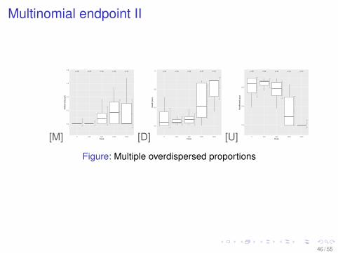
I Nonclin example: in a reproductive toxicity experiment nijfemales are treated within the dose groups (and zero-dosecontrol) and the health status of each pup within a singlefemale is classified into unaffected, malformed or death.

I Up to now approaches for simultaneous inference foroverdispersed multinomial vectors seems to be notavailable.

I Approach I : splitting into the 3 proportionspd = xdeath/xunaffected ,...,..., followed by a trend test forcorrelated overdispersed binary endpoints

45 / 55

Multinomial endpoint II

[M]

n=28 n=26 n=26 n=23 n=22

0.0

0.2

0.4

0.6

0.8

0 250 500 1000 1500Dose

Mal

form

ed p

ups

[D]

n=28 n=26 n=26 n=23 n=22

0.0

0.4

0.8

1.2

0 250 500 1000 1500Dose

Dea

th p

ups

[U]

n=28 n=26 n=26 n=23 n=22

0.0

0.4

0.8

0 250 500 1000 1500Dose

Une

ffect

ed p

ups

Figure: Multiple overdispersed proportions

46 / 55

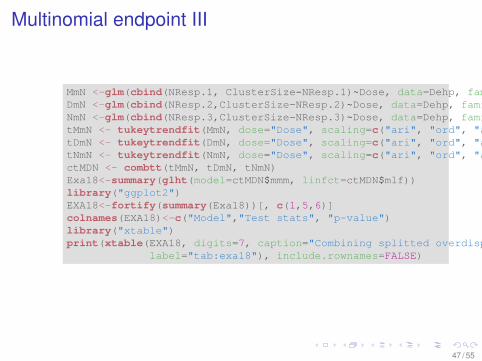
Multinomial endpoint III

MmN <-glm(cbind(NResp.1, ClusterSize-NResp.1)~Dose, data=Dehp, family= quasibinomial(link="logit"))DmN <-glm(cbind(NResp.2,ClusterSize-NResp.2)~Dose, data=Dehp, family= quasibinomial(link="logit"))NmN <-glm(cbind(NResp.3,ClusterSize-NResp.3)~Dose, data=Dehp, family= quasibinomial(link="logit"))tMmN <- tukeytrendfit(MmN, dose="Dose", scaling=c("ari", "ord", "arilog"))tDmN <- tukeytrendfit(DmN, dose="Dose", scaling=c("ari", "ord", "arilog"))tNmN <- tukeytrendfit(NmN, dose="Dose", scaling=c("ari", "ord", "arilog"))ctMDN <- combtt(tMmN, tDmN, tNmN)Exa18<-summary(glht(model=ctMDN$mmm, linfct=ctMDN$mlf))library("ggplot2")EXA18<-fortify(summary(Exa18))[, c(1,5,6)]colnames(EXA18)<-c("Model","Test stats", "p-value")library("xtable")print(xtable(EXA18, digits=7, caption="Combining splitted overdispersed multinomials into multiple binomials",

label="tab:exa18"), include.rownames=FALSE)

47 / 55

Multinomial endpoint IV

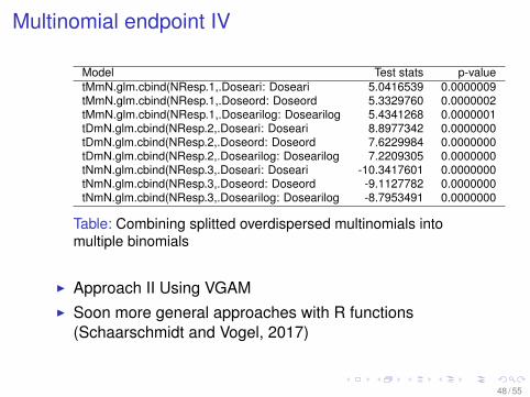
Model Test stats p-valuetMmN.glm.cbind(NResp.1,.Doseari: Doseari 5.0416539 0.0000009tMmN.glm.cbind(NResp.1,.Doseord: Doseord 5.3329760 0.0000002tMmN.glm.cbind(NResp.1,.Dosearilog: Dosearilog 5.4341268 0.0000001tDmN.glm.cbind(NResp.2,.Doseari: Doseari 8.8977342 0.0000000tDmN.glm.cbind(NResp.2,.Doseord: Doseord 7.6229984 0.0000000tDmN.glm.cbind(NResp.2,.Dosearilog: Dosearilog 7.2209305 0.0000000tNmN.glm.cbind(NResp.3,.Doseari: Doseari -10.3417601 0.0000000tNmN.glm.cbind(NResp.3,.Doseord: Doseord -9.1127782 0.0000000tNmN.glm.cbind(NResp.3,.Dosearilog: Dosearilog -8.7953491 0.0000000

Table: Combining splitted overdispersed multinomials intomultiple binomials

I Approach II Using VGAMI Soon more general approaches with R functions

(Schaarschmidt and Vogel, 2017)

48 / 55

Trends in epidemiology: individual random dose levelsI

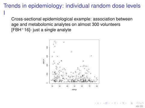
Cross-sectional epidemiological example: association betweenage and metabolomic analytes on almost 300 volunteers[FBH+16]- just a single analyte

20 30 40 50 60 70 80

020

040

060

080

0

dd$Age

dd$X

24

49 / 55

Trends in epidemiology: individual random dose levelsII

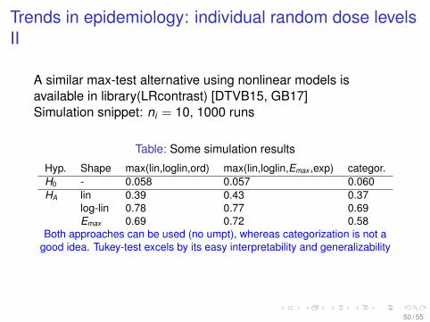
A similar max-test alternative using nonlinear models isavailable in library(LRcontrast) [DTVB15, GB17]Simulation snippet: ni = 10, 1000 runs

Table: Some simulation results

Hyp. Shape max(lin,loglin,ord) max(lin,loglin,Emax ,exp) categor.H0 - 0.058 0.057 0.060HA lin 0.39 0.43 0.37

log-lin 0.78 0.77 0.69Emax 0.69 0.72 0.58

Both approaches can be used (no umpt), whereas categorization is not agood idea. Tukey-test excels by its easy interpretability and generalizability

50 / 55

Further general mmm applications I

I Multiple normal distributed endpoints in multi-arm trials:Dunnett-type sCI

I Multiple binary endpointsI Multiple binary endpoints in multi-arm trials: Williams-type

trend testI Multiple regression models in genetic association test

[ARH17]I Composite binary endpoints [MRH16]I Subgroup analysis with claim for total, targeted and

complementary populations (soon Vogel et al.)I Inference on dose (randomized) and time (dependent)

[PPR15]

51 / 55

Take home message I

I Trend tests for several possible shapes are available with inglmm framework→ rather relevant for nonclin and clintrials and epidemiological studies

I TukeyWilliams trend test can be recommended: R libraryavailable, simple interpretation

I Extension to model II of regressionI Flexibility is amazing: see vignetteI Use confidence intervals! Interpret the effect size first, for

the simple slopesI Comparison with nonlinear models (incl. model averaging

resp. model selection) neededI Basic property of mmm: no explicit formulation of RI The Tukey trend approach follows KISS

52 / 55

References I[AC98] A. Agresti and B. A. Coull. Approximate is better than "exact" for interval estimation of binomial

proportions. American Statistician, 52(2):119–126, May 1998.

[ARH17] Kitsche A., C. Ritz, and LA. Hothorn. A general framework for the evaluation of genetic associationstudies using multiple marginal models. Human Heredity, 2017.

[Arm55] P. Armitage. Tests for linear trends in proportions and frequencies. Biometrics, 11(3):375–386, 1955.

[AXL11] Girish Aras, Allen Xue, and Thomas Liu. Tukey’s contrast test versus two-sample test in adose-response clinical trial. Statistics In Biopharmaceutical Research, 3(1):31–39, February 2011.

[Bar59] D. J. Bartholomew. A test of homogeneity for ordered alternatives. Biometrika, 46(1-2):36–48, 1959.

[BM00] E. Brunner and U. Munzel. The nonparametric Behrens-Fisher problem: Asymptotic theory and asmall-sample approximation. Biometrical Journal, 42(1):17–25, 2000.

[Bre06] Frank Bretz. An extension of the Williams trend test to general unbalanced linear models. ComputionalStatistics and Data Analysis, 50(7):1735–1748, 2006.

[DBGH04] G. Dilba, E. Bretz, V. Guiard, and L. A. Hothorn. Simultaneous confidence intervals for ratios withapplications to the comparison of several treatments with a control. Method Inform Med, 43(5):465–469,2004.

[DSH07] G. Dilba, F. Schaarschmidt, and L.A. Hothorn. Inferences for ratios of normal means. R News, 7:20–23,2007.

[DTVB15] H. Dette, S. Titoff, S. Volgushev, and F. Bretz. Dose response signal detection under model uncertainty.Biometrics, 71(4):996–1008, December 2015.

[Dun55] C. W. Dunnett. A multiple comparison procedure for comparing several treatments with a control. J AmStat Assoc, 50(272):1096–1121, 1955.

[F.17] Schaarschmidt F. R package tukeytrend. Technical report, LUH, 2017.

[FBH+16] L. Frommherz, A. Bub, E. Hummel, M. J. Rist, A. Roth, B. Watzl, and S. E. Kulling. Age-related changesof plasma bile acid concentrations in healthy adults-results from the cross-sectional karmen study. PlosOne, 11(4):e0153959, April 2016.

[GB17] G. Gutjahr and B. Bornkamp. Likelihood ratio tests for a dose-response effect using multiple nonlinearregression models. Biometrics, 73(1):197–205, March 2017.

53 / 55

References II[Ger16] D. Gerhard. Simultaneous small sample inference for linear combinations of generalized linear model

parameters. Communications in Statistics-simulation and Computation, 45(8):2678–2690, 2016.

[Hay13] A. J. Hayter. Inferences on the difference between future observations for comparing two treatments.Journal of Applied Statistics, 40(4):887–900, APR 1 2013.

[HH08] M. Hasler and L. A. Hothorn. Multiple contrast tests in the presence of heteroscedasticity. BiometricalJournaI, 50(5, SI):793–800, OCT 2008.

[HH12] E. Herberich and L.A. Hothorn. Statistical evaluation of mortality in long-term carcinogenicity bioassaysusing a Williams-type procedure. Regul Toxicol Pharm, 64:26–34, 2012.

[HH13] M. Hasler and L. A. Hothorn. Simultaneous confidence intervals on multivariate non-inferiority. StatisticsIn Medicine, 32(10):1720–1729, May 2013.

[Hot] Hothorn, L.A. Statistics in Toxicology-using R (2015).

[HYH11] C. Hirotsu, S. Yamamoto, and L.A. Hothorn. Estimating the dose-response pattern by the maximalcontrast type test approach. Statistics in Biopharmaceutical Research, 3(1):40–53, February 2011.

[KH12a] F. Konietschke and L.A. Hothorn. Evaluation of toxicological studies using a non-parametric Shirley-typetrend test for comparing several dose levels with a control group. Stat Biopharm Res, 4:14–27, 2012.

[KH12b] F. Konietschke and L.A. Hothorn. Rank-based multiple test procedures and simultaneous confidenceintervals. Electron J Stat, 6:738–759, 2012.

[KPSH15] F. Konietschke, M. Placzek, F. Schaarschmidt, and L.A. Hothorn. nparcomp: An R software package fornonparametric multiple comparisons and simultaneous confidence intervals. Journal of StatisticalSoftware, 64(9):1–17, 2015.

[KYY+16] T. Kimura, K. Yasuda, R. Yamamoto, T. Soga, H. Rakugi, T. Hayashi, and Y. Isaka. Identification ofbiomarkers for development of end-stage kidney disease in chronic kidney disease by metabolomicprofiling. Scientific Reports, 6:26138, May 2016.

[MRH16] GrosseRuse M., C. Ritz, and L.A. Hothorn. Simultaneous inference of a binary composite endpoint andits components. J. Biopharm Statist, 2016.

[NTP] National Toxicology Program. 13 Weeks gavage study on female F344 rats administered with Sodiumdichromate dihydrate (VI) (CASRN: 7789-12-0, Study Number: C20114,TDMS Number:2011402.

54 / 55

References III

[PH16] P. Pallmann and L. A. Hothorn. Analysis of means: a generalized approach using r. Journal of AppliedStatistics, 43(8):1541–1560, June 2016.

[PPR15] P: Pallmann, M. Pretorius, and C. Ritz. Simultaneous comparisons of treatments at multiple time points:Combined marginal models versus joint modeling. Statistical Methods in Medical Research, 2015.

[PRB12] Christian Bressen Pipper, Christian Ritz, and Hans Bisgaard. A versatile method for confirmatoryevaluation of the effects of a covariate in multiple models. Journal of the Royal Statistical Society SeriesC-applied Statistics, 61:315–326, 2012.

[Ryu09] E.J. Ryu. Simultaneous confidence intervals using ordinal effect measures for ordered categoricaloutcomes. Statistics in Medicine, 28(25):3179–3188, November 2009.

[SBH09] F. Schaarschmidt, E. Biesheuvel, and L. A. Hothorn. Asymptotic simultaneous confidence intervals formany-to-one comparisons of binary proportions in randomized clinical trials. Journal ofBiopharmaceutical Statistics, 19(2):292–310, 2009.

[Sch13] F. Schaarschmidt. Simultaneous confidence intervals for multiple comparisons among expected valuesof log-normal variables. Computational Statistics and Data Analysis, 58:265–275, FEB 2013.

[SGV16] F. Schaarschmidt, D. Gerhard, and C. Vogel. Simultaneous confidence intervals for comparisons ofseveral multinomial samples. CSDA, 2016.

[SSH08a] F. Schaarschmidt, M. Sill, and L. A. Hothorn. Approximate simultaneous confidence intervals for multiplecontrasts of binomial proportions. Biometrical Journal, 50(5):782–792, October 2008.

[SSH08b] F. Schaarschmidt, M. Sill, and L. A. Hothorn. Poly-k-trend tests for survival adjusted analysis of tumorrates formulated as approximate multiple contrast test. J Biopharm Stat, 18(5):934–948, 2008.

[TCH85] J. W. Tukey, J. L. Ciminera, and J. F. Heyse. Testing the statistical certainty of a response to increasingdoses of a drug. Biometrics, 41(1):295–301, 1985.

[Wil71] D A Williams. A test for differences between treatment means when several dose levels are comparedwith a zero dose control. Biometrics, 27(1):103–117, 1971.

55 / 55