Embed Size (px)
Citation preview

. . . . . .
.
......
Domain Decomposition Preconditionersfor Isogeometric Discretizations
Luca F. Pavarino, Universita di Milano, Italy
Lorenzo Beirao da Veiga, Universita di Milano, ItalyDurkbin Cho, Dongguk University, Seoul, South Korea
Simone Scacchi, Universita di Milano, ItalyOlof B. Widlund, Courant Institute, NYU, USA
Stefano Zampini, KAUST, Saudi Arabia
DD 23ICC - Jeju, Jeju Island, South Korea, July 6-10, 2015
L. Beirao da Veiga, D. Cho, L. F. Pavarino, S. Scacchi Isogeometric Domain Decomposition Preconditioners
. . . . . .
.. IGA Motivations
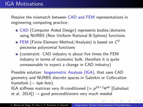
Resolve the mismatch between CAD and FEM representations inengineering computing practice:
CAD (Computer Aided Design) represents bodies/domainsusing NURBS (Non Uniform Rational B-Splines) functions
FEM (Finite Element Method/Analysis) is based on C 0
piecewise polynomial functions
(constraint: CAD industry is about five times the FEMindustry in terms of economic bulk, therefore it is quiteunreasonable to expect a change in CAD industry)
Possible solution: Isogeometric Analysis (IGA), that uses CADgeometry and NURBS discrete spaces in Galerkin or Collocationframefork (∼ hpk-fem).IGA stiffness matrices very ill-conditioned (≈ p2d+24pd [Gahalautet al. 2014]) → good preconditioners very much needed
L. Beirao da Veiga, D. Cho, L. F. Pavarino, S. Scacchi Isogeometric Domain Decomposition Preconditioners
. . . . . .
.. IGA Motivations
Resolve the mismatch between CAD and FEM representations inengineering computing practice:
CAD (Computer Aided Design) represents bodies/domainsusing NURBS (Non Uniform Rational B-Splines) functions
FEM (Finite Element Method/Analysis) is based on C 0
piecewise polynomial functions
(constraint: CAD industry is about five times the FEMindustry in terms of economic bulk, therefore it is quiteunreasonable to expect a change in CAD industry)
Possible solution: Isogeometric Analysis (IGA), that uses CADgeometry and NURBS discrete spaces in Galerkin or Collocationframefork (∼ hpk-fem).
IGA stiffness matrices very ill-conditioned (≈ p2d+24pd [Gahalautet al. 2014]) → good preconditioners very much needed
L. Beirao da Veiga, D. Cho, L. F. Pavarino, S. Scacchi Isogeometric Domain Decomposition Preconditioners
. . . . . .
.. IGA Motivations
Resolve the mismatch between CAD and FEM representations inengineering computing practice:
CAD (Computer Aided Design) represents bodies/domainsusing NURBS (Non Uniform Rational B-Splines) functions
FEM (Finite Element Method/Analysis) is based on C 0
piecewise polynomial functions
(constraint: CAD industry is about five times the FEMindustry in terms of economic bulk, therefore it is quiteunreasonable to expect a change in CAD industry)
Possible solution: Isogeometric Analysis (IGA), that uses CADgeometry and NURBS discrete spaces in Galerkin or Collocationframefork (∼ hpk-fem).IGA stiffness matrices very ill-conditioned (≈ p2d+24pd [Gahalautet al. 2014]) → good preconditioners very much needed
L. Beirao da Veiga, D. Cho, L. F. Pavarino, S. Scacchi Isogeometric Domain Decomposition Preconditioners
. . . . . .
.. Some IGA DD references
IGA very active emerging field, growing literature, see e.g.J. A. Cottrell, T. J. R. Hughes, Y. Bazilevs, Isogeometric Analysis. Toward
integration of CAD and FEA, Wiley, 2009 and subsequent works
But few references for IGA iterative solvers are available:
Overlapping Schwarz [Beirao da Veiga, Cho, LFP, Scacchi, SINUM 2012,CMAME 2013]
BDDC [Beirao da Veiga, Cho, LFP, Scacchi, M3AN 2013], [Beirao daVeiga, LFP, Scacchi, Widlund, Zampini, SISC 2014]
IETI [Kleiss, Pechstein, Juttler, Tomar, CMAME 2012]
Multigrid [Gahalaut, Kraus, Tomar, CMAME 2012], [Takacs et al. 2015]
BPX [Buffa, Harbrecht, Kunoth, Sangalli, CMAME 2013]
...
L. Beirao da Veiga, D. Cho, L. F. Pavarino, S. Scacchi Isogeometric Domain Decomposition Preconditioners

. . . . . .
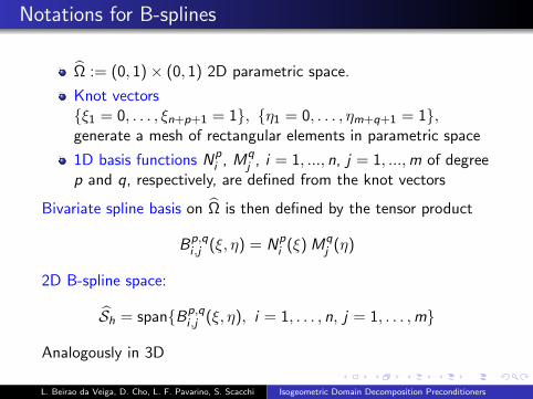
.. Notations for B-splines
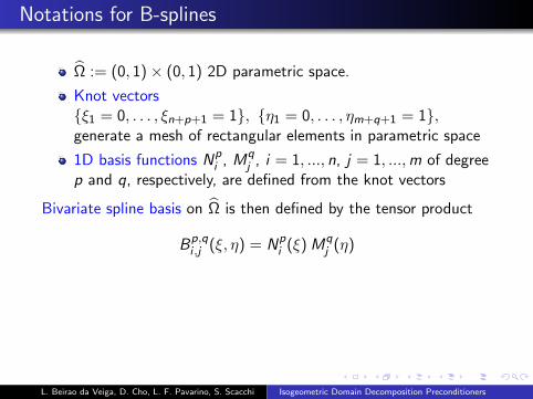
Ω := (0, 1)× (0, 1) 2D parametric space.
Knot vectorsξ1 = 0, . . . , ξn+p+1 = 1, η1 = 0, . . . , ηm+q+1 = 1,generate a mesh of rectangular elements in parametric space
1D basis functions Npi , M
qj , i = 1, ..., n, j = 1, ...,m of degree
p and q, respectively, are defined from the knot vectors
Bivariate spline basis on Ω is then defined by the tensor product
Bp,qi ,j (ξ, η) = Np
i (ξ)Mqj (η)
2D B-spline space:
Sh = spanBp,qi ,j (ξ, η), i = 1, . . . , n, j = 1, . . . ,m
Analogously in 3D
L. Beirao da Veiga, D. Cho, L. F. Pavarino, S. Scacchi Isogeometric Domain Decomposition Preconditioners
. . . . . .
.. Notations for B-splines
Ω := (0, 1)× (0, 1) 2D parametric space.
Knot vectorsξ1 = 0, . . . , ξn+p+1 = 1, η1 = 0, . . . , ηm+q+1 = 1,generate a mesh of rectangular elements in parametric space
1D basis functions Npi , M
qj , i = 1, ..., n, j = 1, ...,m of degree
p and q, respectively, are defined from the knot vectors
Bivariate spline basis on Ω is then defined by the tensor product
Bp,qi ,j (ξ, η) = Np
i (ξ)Mqj (η)
2D B-spline space:
Sh = spanBp,qi ,j (ξ, η), i = 1, . . . , n, j = 1, . . . ,m
Analogously in 3D
L. Beirao da Veiga, D. Cho, L. F. Pavarino, S. Scacchi Isogeometric Domain Decomposition Preconditioners

. . . . . .
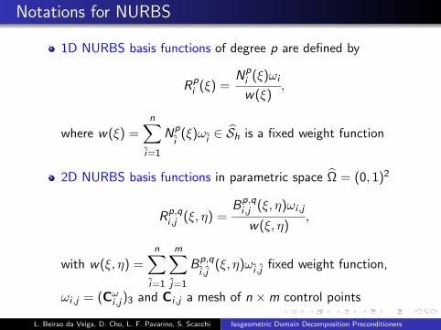
.. Notations for NURBS
1D NURBS basis functions of degree p are defined by
Rpi (ξ) =
Npi (ξ)ωi
w(ξ),
where w(ξ) =n∑
i=1
Np
i(ξ)ωi ∈ Sh is a fixed weight function
2D NURBS basis functions in parametric space Ω = (0, 1)2
Rp,qi ,j (ξ, η) =
Bp,qi ,j (ξ, η)ωi ,j
w(ξ, η),
with w(ξ, η) =n∑
i=1
m∑j=1
Bp,q
i ,j(ξ, η)ωi ,j fixed weight function,
ωi ,j = (Cωi ,j)3 and Ci ,j a mesh of n ×m control points
L. Beirao da Veiga, D. Cho, L. F. Pavarino, S. Scacchi Isogeometric Domain Decomposition Preconditioners
. . . . . .
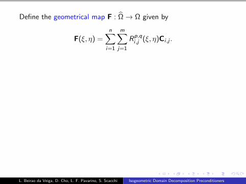
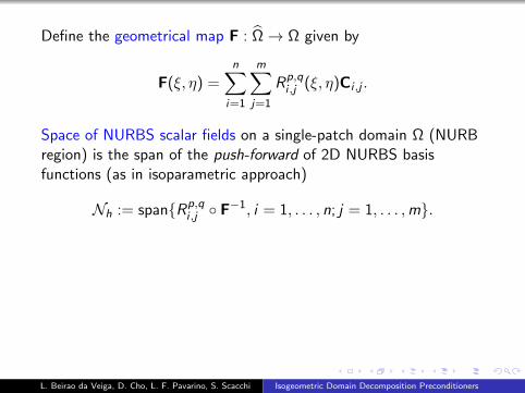
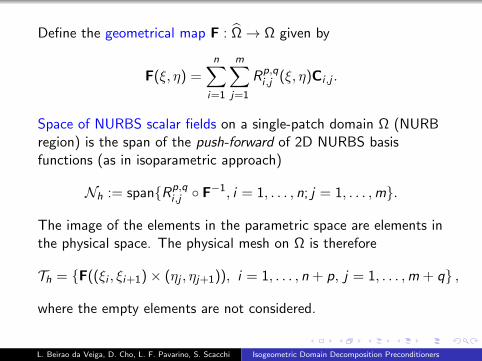
Define the geometrical map F : Ω → Ω given by
F(ξ, η) =n∑
i=1
m∑j=1
Rp,qi ,j (ξ, η)Ci ,j .
Space of NURBS scalar fields on a single-patch domain Ω (NURBregion) is the span of the push-forward of 2D NURBS basisfunctions (as in isoparametric approach)
Nh := spanRp,qi ,j F−1, i = 1, . . . , n; j = 1, . . . ,m.
The image of the elements in the parametric space are elements inthe physical space. The physical mesh on Ω is therefore
Th = F((ξi , ξi+1)× (ηj , ηj+1)), i = 1, . . . , n + p, j = 1, . . . ,m + q ,
where the empty elements are not considered.
L. Beirao da Veiga, D. Cho, L. F. Pavarino, S. Scacchi Isogeometric Domain Decomposition Preconditioners
. . . . . .
Define the geometrical map F : Ω → Ω given by
F(ξ, η) =n∑
i=1
m∑j=1
Rp,qi ,j (ξ, η)Ci ,j .
Space of NURBS scalar fields on a single-patch domain Ω (NURBregion) is the span of the push-forward of 2D NURBS basisfunctions (as in isoparametric approach)
Nh := spanRp,qi ,j F−1, i = 1, . . . , n; j = 1, . . . ,m.
The image of the elements in the parametric space are elements inthe physical space. The physical mesh on Ω is therefore
Th = F((ξi , ξi+1)× (ηj , ηj+1)), i = 1, . . . , n + p, j = 1, . . . ,m + q ,
where the empty elements are not considered.
L. Beirao da Veiga, D. Cho, L. F. Pavarino, S. Scacchi Isogeometric Domain Decomposition Preconditioners

. . . . . .
(Fig. 1.9 from Cottrell et al., Wiley, 2009)From CAD and FEA to Isogeometric Analysis 17
1 765432
1
2
3
4
5
6
7
8
Index space
1,2 ,3,4 ,5 ,6 ,7 0, 0, 0, 1/2, 1, 1, 1
1,2 ,3,4 ,5 ,6 ,7 ,8 0, 0, 0, 1/3, 2/3, 1, 1, 1
Knot vectors
0 1
1
2/3
1/3
01/2
N1
N4N
2N
3
M1M
2M
3M
4
M5
2
-1 1-1
1
Parameter
space
Parent
element
0 11/2
Rij
, w
ijN
i()M
j()
wi jN
i()M
j()
i , j
Integration is
performed on the
parent element12/3
1/3
0
x
y
z
Control point Bij
3
Control mesh
Physical mesh
Physical
space
S , BijRij
, i, j
Figure 1.9 Schematic illustration of NURBS paraphernalia for a one-patch surface model. Open knot
vectors and quadratic C 1-continuous basis functions are used. Complex multi-patch geometries may
be constructed by assembling control meshes as in standard finite element analysis. Also depicted are
C1-quadratic (p 2) basis functions determined by the knot vectors. Basis functions are multiplied by
control points and summed to construct geometrical objects, in this case a surface in 3. The procedure
used to define basis functions from knot vectors will be described in detail in Chapter 2.
L. Beirao da Veiga, D. Cho, L. F. Pavarino, S. Scacchi Isogeometric Domain Decomposition Preconditioners
. . . . . .
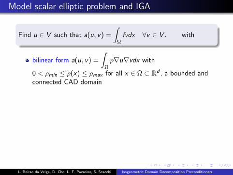
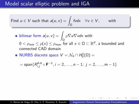
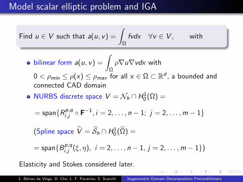
.. Model scalar elliptic problem and IGA
.
......Find u ∈ V such that a(u, v) =
∫Ωfvdx ∀v ∈ V , with
bilinear form a(u, v) =
∫Ωρ∇u∇vdx with
0 < ρmin ≤ ρ(x) ≤ ρmax for all x ∈ Ω ⊂ Rd , a bounded andconnected CAD domain
NURBS discrete space V = Nh ∩ H10 (Ω) =
= spanRp,qi ,j F−1, i = 2, . . . , n − 1; j = 2, . . . ,m − 1
(Spline space V = Sh ∩ H10 (Ω) =
= spanBp,qi ,j (ξ, η), i = 2, . . . , n − 1, j = 2, . . . ,m − 1)
Elasticity and Stokes considered later.
L. Beirao da Veiga, D. Cho, L. F. Pavarino, S. Scacchi Isogeometric Domain Decomposition Preconditioners
. . . . . .
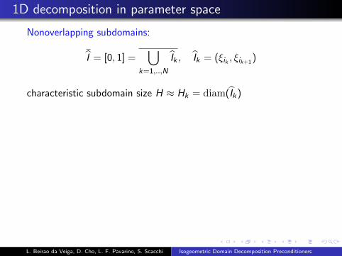
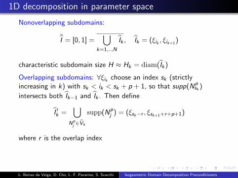
.. 1D decomposition in parameter space
Nonoverlapping subdomains:
I = [0, 1] =∪
k=1,..,N
Ik , Ik = (ξik , ξik+1)
characteristic subdomain size H ≈ Hk = diam(Ik)
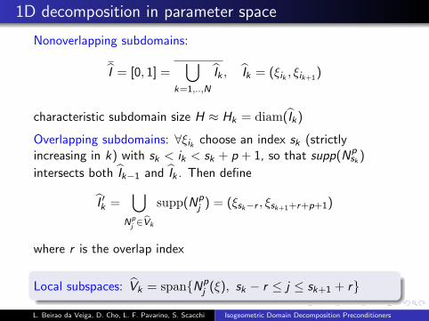
Overlapping subdomains: ∀ξik choose an index sk (strictlyincreasing in k) with sk < ik < sk + p + 1, so that supp(Np
sk )
intersects both Ik−1 and Ik . Then define
I ′k =∪
Npj ∈Vk
supp(Npj ) = (ξsk−r , ξsk+1+r+p+1)
where r is the overlap index
.
......Local subspaces: Vk = spanNpj (ξ), sk − r ≤ j ≤ sk+1 + r
L. Beirao da Veiga, D. Cho, L. F. Pavarino, S. Scacchi Isogeometric Domain Decomposition Preconditioners
. . . . . .
.. 1D decomposition in parameter space
Nonoverlapping subdomains:
I = [0, 1] =∪
k=1,..,N
Ik , Ik = (ξik , ξik+1)
characteristic subdomain size H ≈ Hk = diam(Ik)
Overlapping subdomains: ∀ξik choose an index sk (strictlyincreasing in k) with sk < ik < sk + p + 1, so that supp(Np
sk )
intersects both Ik−1 and Ik . Then define
I ′k =∪
Npj ∈Vk
supp(Npj ) = (ξsk−r , ξsk+1+r+p+1)
where r is the overlap index
.
......Local subspaces: Vk = spanNpj (ξ), sk − r ≤ j ≤ sk+1 + r
L. Beirao da Veiga, D. Cho, L. F. Pavarino, S. Scacchi Isogeometric Domain Decomposition Preconditioners
. . . . . .
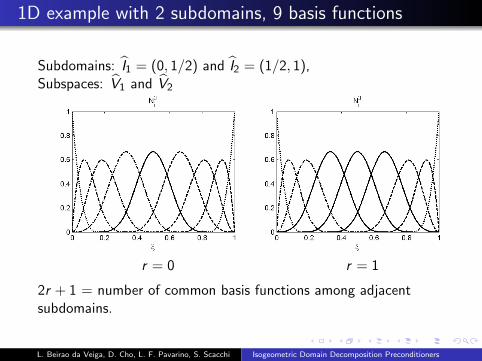
.. 1D example with 2 subdomains, 9 basis functions
Subdomains: I1 = (0, 1/2) and I2 = (1/2, 1),Subspaces: V1 and V2
r = 0 r = 1
2r + 1 = number of common basis functions among adjacentsubdomains.
L. Beirao da Veiga, D. Cho, L. F. Pavarino, S. Scacchi Isogeometric Domain Decomposition Preconditioners

. . . . . .
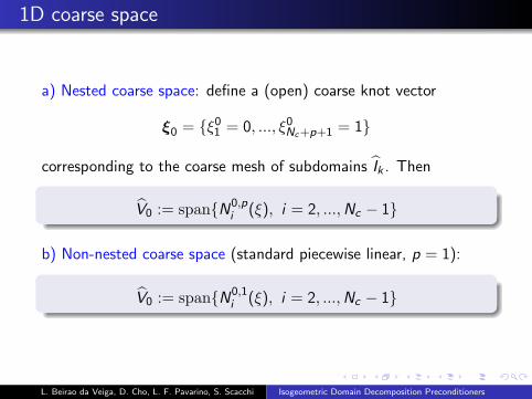
.. 1D coarse space
a) Nested coarse space: define a (open) coarse knot vector
ξ0 = ξ01 = 0, ..., ξ0Nc+p+1 = 1
corresponding to the coarse mesh of subdomains Ik . Then.
...... V0 := spanN0,pi (ξ), i = 2, ...,Nc − 1
b) Non-nested coarse space (standard piecewise linear, p = 1):.
...... V0 := spanN0,1i (ξ), i = 2, ...,Nc − 1
L. Beirao da Veiga, D. Cho, L. F. Pavarino, S. Scacchi Isogeometric Domain Decomposition Preconditioners
. . . . . .
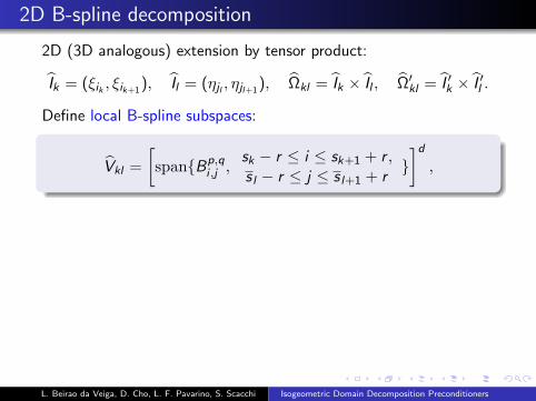
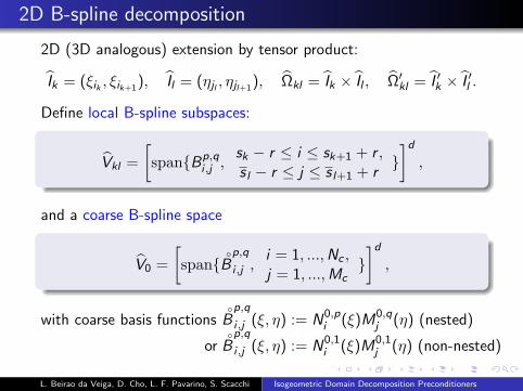
.. 2D B-spline decomposition
2D (3D analogous) extension by tensor product:
Ik = (ξik , ξik+1), Il = (ηjl , ηjl+1
), Ωkl = Ik × Il , Ω′kl = I ′k × I ′l .
Define local B-spline subspaces:.
......Vkl =
[spanBp,q
i ,j ,sk − r ≤ i ≤ sk+1 + r ,s l − r ≤ j ≤ s l+1 + r
]d
,
and a coarse B-spline space.
......V0 =
[span
B
p,q
i ,j ,i = 1, ...,Nc ,j = 1, ...,Mc
]d
,
with coarse basis functionsB
p,q
i ,j (ξ, η) := N0,pi (ξ)M0,q
j (η) (nested)
orB
p,q
i ,j (ξ, η) := N0,1i (ξ)M0,1
j (η) (non-nested)
L. Beirao da Veiga, D. Cho, L. F. Pavarino, S. Scacchi Isogeometric Domain Decomposition Preconditioners
. . . . . .
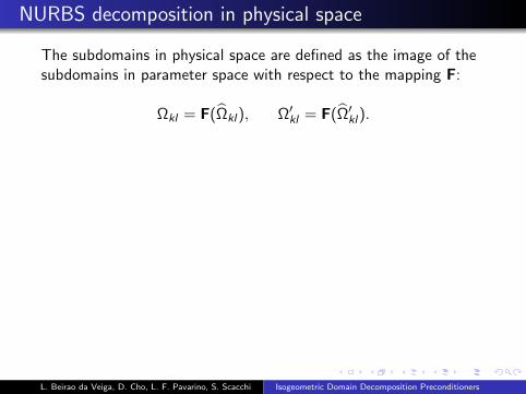
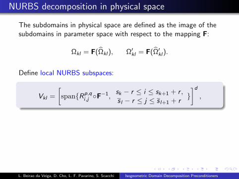
.. NURBS decomposition in physical space
The subdomains in physical space are defined as the image of thesubdomains in parameter space with respect to the mapping F:
Ωkl = F(Ωkl), Ω′kl = F(Ω′
kl).
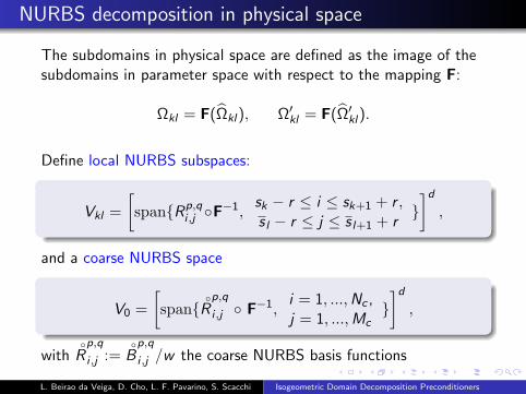
Define local NURBS subspaces:.
......Vkl =
[spanRp,q
i ,j F−1,sk − r ≤ i ≤ sk+1 + r ,s l − r ≤ j ≤ s l+1 + r
]d
,
and a coarse NURBS space.
......V0 =
[span
Rp,q
i ,j F−1,i = 1, ...,Nc ,j = 1, ...,Mc
]d
,
withRp,q
i ,j :=B
p,q
i ,j /w the coarse NURBS basis functions
L. Beirao da Veiga, D. Cho, L. F. Pavarino, S. Scacchi Isogeometric Domain Decomposition Preconditioners
. . . . . .
.. NURBS decomposition in physical space
The subdomains in physical space are defined as the image of thesubdomains in parameter space with respect to the mapping F:
Ωkl = F(Ωkl), Ω′kl = F(Ω′
kl).
Define local NURBS subspaces:.
......Vkl =
[spanRp,q
i ,j F−1,sk − r ≤ i ≤ sk+1 + r ,s l − r ≤ j ≤ s l+1 + r
]d
,
and a coarse NURBS space.
......V0 =
[span
Rp,q
i ,j F−1,i = 1, ...,Nc ,j = 1, ...,Mc
]d
,
withRp,q
i ,j :=B
p,q
i ,j /w the coarse NURBS basis functions
L. Beirao da Veiga, D. Cho, L. F. Pavarino, S. Scacchi Isogeometric Domain Decomposition Preconditioners
. . . . . .
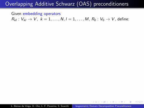
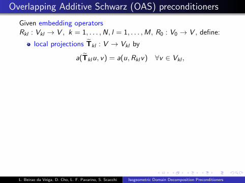
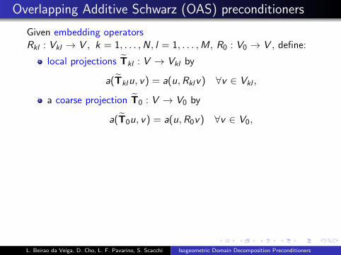
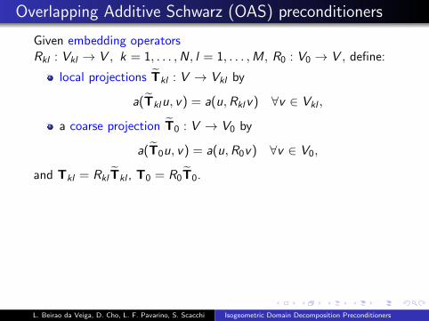
.. Overlapping Additive Schwarz (OAS) preconditioners
Given embedding operatorsRkl : Vkl → V , k = 1, . . . ,N, l = 1, . . . ,M, R0 : V0 → V , define:
local projections Tkl : V → Vkl by
a(Tklu, v) = a(u,Rklv) ∀v ∈ Vkl ,
a coarse projection T0 : V → V0 by
a(T0u, v) = a(u,R0v) ∀v ∈ V0,
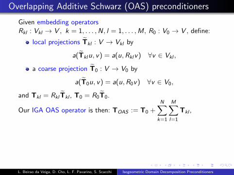
and Tkl = Rkl Tkl , T0 = R0T0.
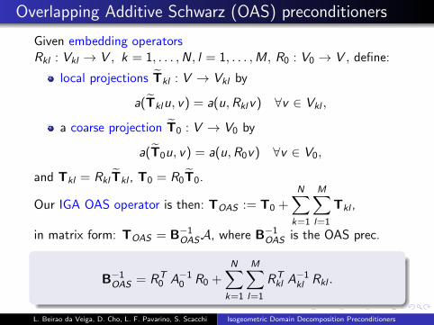
Our IGA OAS operator is then: TOAS := T0 +N∑
k=1
M∑l=1
Tkl ,
in matrix form: TOAS = B−1OASA, where B−1
OAS is the OAS prec..
......
B−1OAS = RT
0 A−10 R0 +
N∑k=1
M∑l=1
RTkl A
−1kl Rkl .
L. Beirao da Veiga, D. Cho, L. F. Pavarino, S. Scacchi Isogeometric Domain Decomposition Preconditioners
. . . . . .
.. Overlapping Additive Schwarz (OAS) preconditioners
Given embedding operatorsRkl : Vkl → V , k = 1, . . . ,N, l = 1, . . . ,M, R0 : V0 → V , define:
local projections Tkl : V → Vkl by
a(Tklu, v) = a(u,Rklv) ∀v ∈ Vkl ,
a coarse projection T0 : V → V0 by
a(T0u, v) = a(u,R0v) ∀v ∈ V0,
and Tkl = Rkl Tkl , T0 = R0T0.
Our IGA OAS operator is then: TOAS := T0 +N∑
k=1
M∑l=1
Tkl ,
in matrix form: TOAS = B−1OASA, where B−1
OAS is the OAS prec..
......
B−1OAS = RT
0 A−10 R0 +
N∑k=1
M∑l=1
RTkl A
−1kl Rkl .
L. Beirao da Veiga, D. Cho, L. F. Pavarino, S. Scacchi Isogeometric Domain Decomposition Preconditioners
. . . . . .
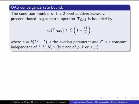
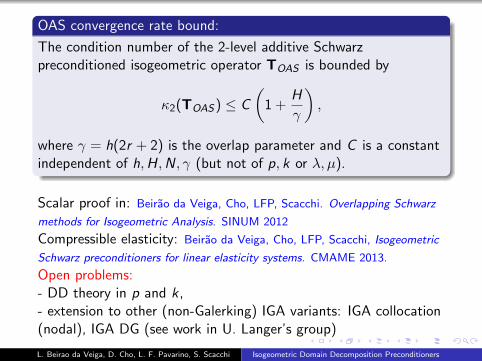
.OAS convergence rate bound:..
......
The condition number of the 2-level additive Schwarzpreconditioned isogeometric operator TOAS is bounded by
κ2(TOAS) ≤ C
(1 +
H
γ
),
where γ = h(2r + 2) is the overlap parameter and C is a constantindependent of h,H,N, γ (but not of p, k or λ, µ).
Scalar proof in: Beirao da Veiga, Cho, LFP, Scacchi. Overlapping Schwarz
methods for Isogeometric Analysis. SINUM 2012
Compressible elasticity: Beirao da Veiga, Cho, LFP, Scacchi, Isogeometric
Schwarz preconditioners for linear elasticity systems. CMAME 2013.
Open problems:- DD theory in p and k,- extension to other (non-Galerking) IGA variants: IGA collocation(nodal), IGA DG (see work in U. Langer’s group)
L. Beirao da Veiga, D. Cho, L. F. Pavarino, S. Scacchi Isogeometric Domain Decomposition Preconditioners
. . . . . .
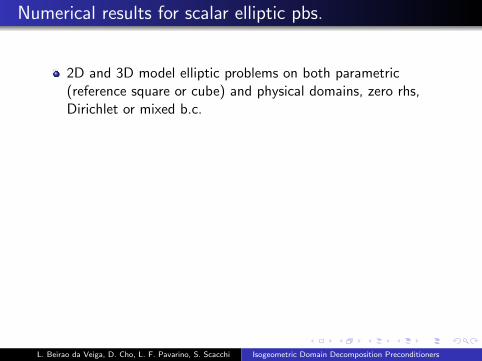
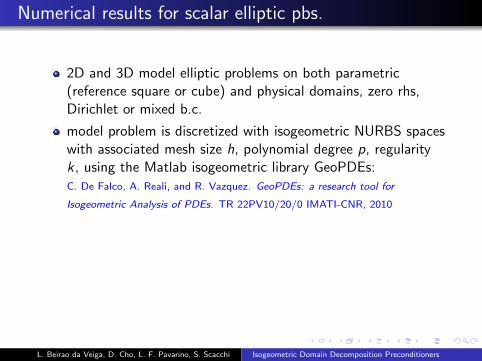
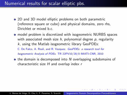
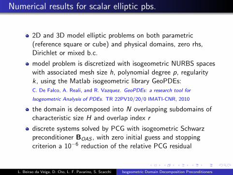
.. Numerical results for scalar elliptic pbs.
2D and 3D model elliptic problems on both parametric(reference square or cube) and physical domains, zero rhs,Dirichlet or mixed b.c.
model problem is discretized with isogeometric NURBS spaceswith associated mesh size h, polynomial degree p, regularityk , using the Matlab isogeometric library GeoPDEs:C. De Falco, A. Reali, and R. Vazquez. GeoPDEs: a research tool for
Isogeometric Analysis of PDEs. TR 22PV10/20/0 IMATI-CNR, 2010
the domain is decomposed into N overlapping subdomains ofcharacteristic size H and overlap index r
discrete systems solved by PCG with isogeometric Schwarzpreconditioner BOAS , with zero initial guess and stoppingcriterion a 10−6 reduction of the relative PCG residual
L. Beirao da Veiga, D. Cho, L. F. Pavarino, S. Scacchi Isogeometric Domain Decomposition Preconditioners
. . . . . .
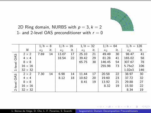
2D Ring domain, NURBS with p = 3, k = 21- and 2-level OAS preconditioner with r = 0
1/h = 8 1/h = 16 1/h = 32 1/h = 64 1/h = 128N κ2 it. κ2 it. κ2 it. κ2 it. κ2 it.
1-level
OAS 2× 2 7.69 14 13.07 17 25.10 21 49.49 30 98.47 41
4× 4 18.54 22 39.42 29 81.28 41 165.02 588× 8 65.75 38 146.45 54 307.67 78
16× 16 255.98 73 5.75e2 10632× 32 1.02e3 146
2-level
OAS 2× 2 7.30 14 6.98 14 11.44 17 20.58 22 38.97 30
4× 4 8.12 18 10.62 20 19.60 23 37.72 328× 8 8.41 19 13.92 21 29.88 27
16× 16 8.32 19 15.50 2232× 32 8.34 19
L. Beirao da Veiga, D. Cho, L. F. Pavarino, S. Scacchi Isogeometric Domain Decomposition Preconditioners
. . . . . .
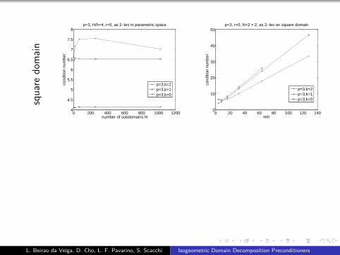
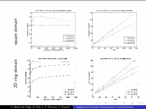
squaredom
ain
0 200 400 600 800 1000 12004
4.5
5
5.5
6
6.5
7
7.5
8
number of subdomains N
cond
ition
num
ber
p=3, H/h=4, r=0, as 2−lev in parametric space
p=3,k=2p=3,k=1p=3,k=0
0 20 40 60 80 100 120 1400
10
20
30
40
50
H/h
cond
ition
num
ber
p=3, r=0, N=2 × 2, as 2−lev on square domain
p=3,k=2p=3,k=1p=3,k=0
2Dringdom
ain
L. Beirao da Veiga, D. Cho, L. F. Pavarino, S. Scacchi Isogeometric Domain Decomposition Preconditioners
. . . . . .
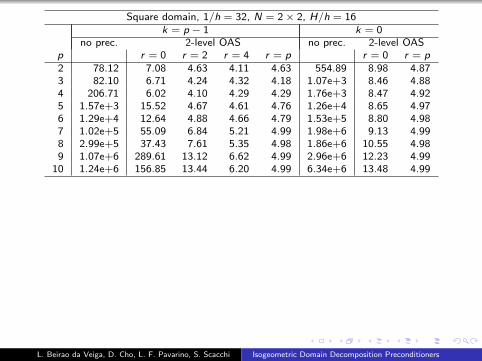
Square domain, 1/h = 32, N = 2× 2, H/h = 16k = p − 1 k = 0
no prec. 2-level OAS no prec. 2-level OASp r = 0 r = 2 r = 4 r = p r = 0 r = p2 78.12 7.08 4.63 4.11 4.63 554.89 8.98 4.873 82.10 6.71 4.24 4.32 4.18 1.07e+3 8.46 4.884 206.71 6.02 4.10 4.29 4.29 1.76e+3 8.47 4.925 1.57e+3 15.52 4.67 4.61 4.76 1.26e+4 8.65 4.976 1.29e+4 12.64 4.88 4.66 4.79 1.53e+5 8.80 4.987 1.02e+5 55.09 6.84 5.21 4.99 1.98e+6 9.13 4.998 2.99e+5 37.43 7.61 5.35 4.98 1.86e+6 10.55 4.989 1.07e+6 289.61 13.12 6.62 4.99 2.96e+6 12.23 4.99
10 1.24e+6 156.85 13.44 6.20 4.99 6.34e+6 13.48 4.99
no prec. 2-level OAS
2 3 4 5 6 7 8 9 1010
0
101
102
103
104
105
106
107
p
cond
. num
ber
k=p−1
k=0
p3
p5
5(p−1)
2 3 4 5 6 7 8 9 1010
0
101
102
103
p
cond
. num
ber
k=p−1, r=0
k=0 o p−1, r=pk=p−1, r=2
k=p−1, r=0
L. Beirao da Veiga, D. Cho, L. F. Pavarino, S. Scacchi Isogeometric Domain Decomposition Preconditioners
. . . . . .
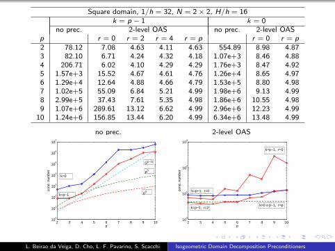
Square domain, 1/h = 32, N = 2× 2, H/h = 16k = p − 1 k = 0
no prec. 2-level OAS no prec. 2-level OASp r = 0 r = 2 r = 4 r = p r = 0 r = p2 78.12 7.08 4.63 4.11 4.63 554.89 8.98 4.873 82.10 6.71 4.24 4.32 4.18 1.07e+3 8.46 4.884 206.71 6.02 4.10 4.29 4.29 1.76e+3 8.47 4.925 1.57e+3 15.52 4.67 4.61 4.76 1.26e+4 8.65 4.976 1.29e+4 12.64 4.88 4.66 4.79 1.53e+5 8.80 4.987 1.02e+5 55.09 6.84 5.21 4.99 1.98e+6 9.13 4.998 2.99e+5 37.43 7.61 5.35 4.98 1.86e+6 10.55 4.989 1.07e+6 289.61 13.12 6.62 4.99 2.96e+6 12.23 4.99
10 1.24e+6 156.85 13.44 6.20 4.99 6.34e+6 13.48 4.99
no prec. 2-level OAS
2 3 4 5 6 7 8 9 1010
0
101
102
103
104
105
106
107
p
cond
. num
ber
k=p−1
k=0
p3
p5
5(p−1)
2 3 4 5 6 7 8 9 1010
0
101
102
103
p
cond
. num
ber
k=p−1, r=0
k=0 o p−1, r=pk=p−1, r=2
k=p−1, r=0
L. Beirao da Veiga, D. Cho, L. F. Pavarino, S. Scacchi Isogeometric Domain Decomposition Preconditioners
. . . . . .
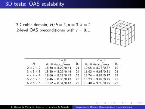
.. 3D tests: OAS scalability
3D cubic domain, H/h = 4, p = 3, k = 22-level OAS preconditioner with r = 0, 1
r = 0 r = 1N κ2 = λMAX /λmin it. κ2 = λMAX /λmin it.
2× 2× 2 18.60 = 8.20/0.44 21 10.05 = 8.78/0.87 193× 3× 3 18.80 = 8.26/0.44 24 11.92 = 9.63/0.81 214× 4× 4 19.66 = 8.29/0.42 25 12.74 = 9.84/0.77 225× 5× 5 19.46 = 8.30/0.43 25 13.23 = 9.92/0.75 236× 6× 6 19.52 = 8.31/0.43 25 13.40 = 9.99/0.75 23
L. Beirao da Veiga, D. Cho, L. F. Pavarino, S. Scacchi Isogeometric Domain Decomposition Preconditioners
. . . . . .
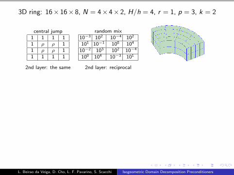
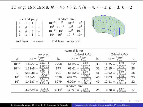
3D ring: 16× 16× 8, N = 4× 4× 2, H/h = 4, r = 1, p = 3, k = 2
central jump1 1 1 11 ρ ρ 11 ρ ρ 11 1 1 1
random mix10−3 102 10−4 102
101 10−1 100 104
10−2 103 102 10−4
100 104 10−3 101
2nd layer: the same 2nd layer: reciprocal
central jumpno prec. 1-level OAS 2-level OAS
ρ κ2 = λMAXλmin
it. κ2 = λMAXλmin
it. κ2 = λMAXλmin
it.
10−4 1.42e7 = 6.00e−14.24e−8
7258 61.65 = 8.001.30e−1
33 11.75 = 8.787.49e−1
22
10−2 1.11e5 = 6.00e−15.41e−6
873 61.61 = 8.001.30e−1
36 12.15 = 8.787.23e−1
25
1 543.38 = 7.94e−11.46e−3
101 65.82 = 8.001.22e−1
41 13.92 = 8.896.39e−1
26
102 1.15e5 = 50.304.39e−4
1030 682.26 = 8.001.17e−2
40 12.03 = 8.937.42e−1
23
104 1.48e7 = 5.01e33.38e−4
8279 6.09e4 = 8.001.31e−4
49 12.11 = 8.937.37e−1
22
random mix3.26e9 = 6.56e3
2.01e−6> 104 30.91 = 8.00
2.59e−125 10.70 = 8.67
8.10e−117
L. Beirao da Veiga, D. Cho, L. F. Pavarino, S. Scacchi Isogeometric Domain Decomposition Preconditioners
. . . . . .
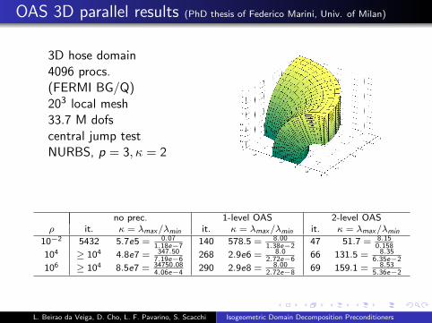
.. OAS 3D parallel results (PhD thesis of Federico Marini, Univ. of Milan)
3D hose domain4096 procs.(FERMI BG/Q)203 local mesh33.7 M dofscentral jump testNURBS, p = 3, κ = 2
no prec. 1-level OAS 2-level OASρ it. κ = λmax/λmin it. κ = λmax/λmin it. κ = λmax/λmin
10−2 5432 5.7e5 = 0.071.18e−7
140 578.5 = 8.001.38e−2
47 51.7 = 8.150.158
104 ≥ 104 4.8e7 = 347.507.19e−6
268 2.9e6 = 8.02.72e−6
66 131.5 = 8.356.35e−2
106 ≥ 104 8.5e7 = 34750.084.06e−4
290 2.9e8 = 8.002.72e−8
69 159.1 = 8.535.36e−2
L. Beirao da Veiga, D. Cho, L. F. Pavarino, S. Scacchi Isogeometric Domain Decomposition Preconditioners
. . . . . .
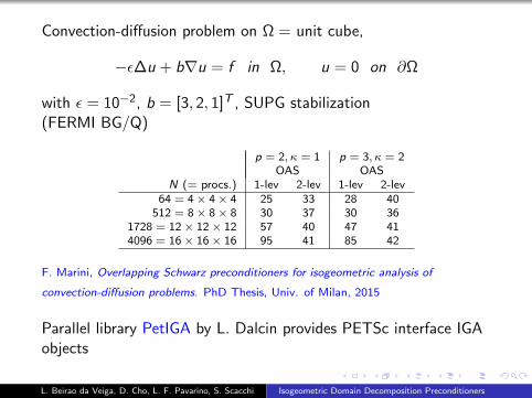
Convection-diffusion problem on Ω = unit cube,
−ϵ∆u + b∇u = f in Ω, u = 0 on ∂Ω
with ϵ = 10−2, b = [3, 2, 1]T , SUPG stabilization(FERMI BG/Q)
p = 2, κ = 1 p = 3, κ = 2OAS OAS
N (= procs.) 1-lev 2-lev 1-lev 2-lev64 = 4× 4× 4 25 33 28 40
512 = 8× 8× 8 30 37 30 361728 = 12× 12× 12 57 40 47 414096 = 16× 16× 16 95 41 85 42
F. Marini, Overlapping Schwarz preconditioners for isogeometric analysis of
convection-diffusion problems. PhD Thesis, Univ. of Milan, 2015
Parallel library PetIGA by L. Dalcin provides PETSc interface IGAobjects
L. Beirao da Veiga, D. Cho, L. F. Pavarino, S. Scacchi Isogeometric Domain Decomposition Preconditioners

. . . . . .
.. Extension to IGA collocation
Same 1D example with 2 subspaces V1, V2 → nodal IGASquares = Greville abscissae associated with knot vector ξ
0 0.2 0.4 0.6 0.8 10
1
ξ
Ni3
0 0.2 0.4 0.6 0.8 10
1
ξ
Ni3
r = 0 r = 1
Beirao da Veiga, Cho, LFP, Scacchi, Overlapping Schwarz preconditioners for
isogeometric collocation methods. CMAME 2014.
Open problems:- DD Collocation IGA for compressible elasticity,- DD Collocation IGA for saddle point formulation
L. Beirao da Veiga, D. Cho, L. F. Pavarino, S. Scacchi Isogeometric Domain Decomposition Preconditioners
. . . . . .
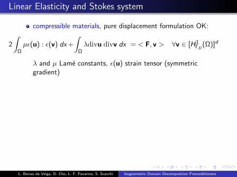
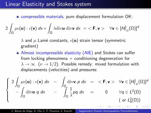
.. Linear Elasticity and Stokes system
compressible materials, pure displacement formulation OK:
2
∫Ωµϵ(u) : ϵ(v) dx+
∫Ωλdivu divv dx = < F, v > ∀v ∈ [H1
ΓD(Ω)]d
λ and µ Lame constants, ϵ(u) strain tensor (symmetricgradient)
Almost incompressible elasticity (AIE) and Stokes can sufferfrom locking phenomena + conditioning degeneration forλ → ∞ (ν → 1/2). Possible remedy: mixed formulation withdisplacements (velocities) and pressures:
2
∫Ωµϵ(u) : ϵ(v) dx −
∫Ωdivv p dx = < F, v > ∀v ∈ [H1
ΓD(Ω)]d
−∫Ωdivu q dx −
∫Ω
1
λpq dx = 0 ∀q ∈ L2(Ω)
( or L20(Ω))
L. Beirao da Veiga, D. Cho, L. F. Pavarino, S. Scacchi Isogeometric Domain Decomposition Preconditioners
. . . . . .
.. Linear Elasticity and Stokes system
compressible materials, pure displacement formulation OK:
2
∫Ωµϵ(u) : ϵ(v) dx+
∫Ωλdivu divv dx = < F, v > ∀v ∈ [H1
ΓD(Ω)]d
λ and µ Lame constants, ϵ(u) strain tensor (symmetricgradient)
Almost incompressible elasticity (AIE) and Stokes can sufferfrom locking phenomena + conditioning degeneration forλ → ∞ (ν → 1/2). Possible remedy: mixed formulation withdisplacements (velocities) and pressures:
2
∫Ωµϵ(u) : ϵ(v) dx −
∫Ωdivv p dx = < F, v > ∀v ∈ [H1
ΓD(Ω)]d
−∫Ωdivu q dx −
∫Ω
1
λpq dx = 0 ∀q ∈ L2(Ω)
( or L20(Ω))
L. Beirao da Veiga, D. Cho, L. F. Pavarino, S. Scacchi Isogeometric Domain Decomposition Preconditioners

. . . . . .
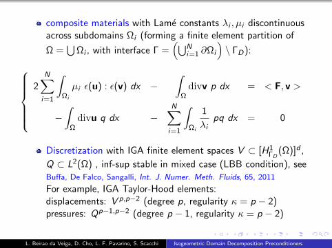
composite materials with Lame constants λi , µi discontinuousacross subdomains Ωi (forming a finite element partition of
Ω =∪
Ωi , with interface Γ =(∪N
i=1 ∂Ωi
)\ ΓD):
2N∑i=1
∫Ωi
µi ϵ(u) : ϵ(v) dx −∫Ωdivv p dx = < F, v >
−∫Ωdivu q dx −
N∑i=1
∫Ωi
1
λipq dx = 0
Discretization with IGA finite element spaces V ⊂ [H1ΓD(Ω)]d ,
Q ⊂ L2(Ω) , inf-sup stable in mixed case (LBB condition), seeBuffa, De Falco, Sangalli, Int. J. Numer. Meth. Fluids, 65, 2011
For example, IGA Taylor-Hood elements:displacements: V p,p−2 (degree p, regularity κ = p − 2)pressures: Qp−1,p−2 (degree p − 1, regularity κ = p − 2)
L. Beirao da Veiga, D. Cho, L. F. Pavarino, S. Scacchi Isogeometric Domain Decomposition Preconditioners
. . . . . .
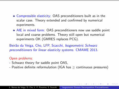
Compressible elasticity: OAS preconditioners built as in thescalar case. Theory extended and confirmed by numericalexperiments.
AIE in mixed form: OAS preconditioners now use saddle pointlocal and coarse problems. Theory still open but numericalexperiments OK (GMRES replaces PCG).
Beirao da Veiga, Cho, LFP, Scacchi, Isogeometric Schwarzpreconditioners for linear elasticity systems. CMAME 2013.
Open problems:- Schwarz theory for saddle point OAS,- Positive definite reformulation (IGA has ≥ continuous pressures)
L. Beirao da Veiga, D. Cho, L. F. Pavarino, S. Scacchi Isogeometric Domain Decomposition Preconditioners
. . . . . .
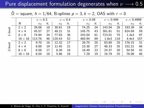
.. Pure displacement formulation degenerates when ν −→ 0.5
Ω = square, h = 1/64, B-splines p = 3, k = 2, OAS with r = 0
ν = 0.3 ν = 0.4 ν = 0.49 ν = 0.499 ν = 0.4999N κ2 it. κ2 it. κ2 it. κ2 it. κ2 it.
1-level 2× 2 29.06 18 30.61 19 74.25 24 143.54 26 193.39 34
4× 4 45.57 27 48.21 31 145.75 43 381.81 51 624.69 598× 8 74.84 34 77.83 38 243.04 61 723.01 75 1.3e3 9716× 16 113.76 46 120.43 52 460.94 89 1.8e3 118 4.4e3 157
2-level 2× 2 9.70 16 12.32 17 26.75 20 83.80 25 176.15 31
4× 4 8.88 19 11.45 21 23.38 27 48.33 35 152.21 468× 8 6.58 17 8.30 18 16.49 23 24.37 30 54.50 4216× 16 6.04 18 5.86 18 7.28 19 16.79 25 76.06 46
0.3 0.35 0.4 0.45 0.510
1
102
103
104
Poisson ratio ν
cond
ition
num
ber
OAS 1 −level
N=2× 2N=4× 4N=8× 8N=16× 16
0.3 0.35 0.4 0.45 0.510
0
101
102
Poisson ratio ν
cond
ition
num
ber
OAS 2 −level
N=2× 2N=4× 4N=8× 8N=16× 16
L. Beirao da Veiga, D. Cho, L. F. Pavarino, S. Scacchi Isogeometric Domain Decomposition Preconditioners
. . . . . .
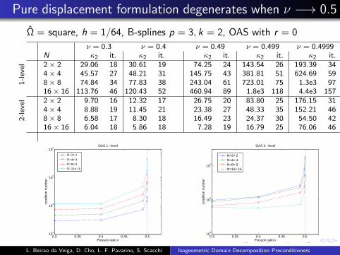
.. Pure displacement formulation degenerates when ν −→ 0.5
Ω = square, h = 1/64, B-splines p = 3, k = 2, OAS with r = 0
ν = 0.3 ν = 0.4 ν = 0.49 ν = 0.499 ν = 0.4999N κ2 it. κ2 it. κ2 it. κ2 it. κ2 it.
1-level 2× 2 29.06 18 30.61 19 74.25 24 143.54 26 193.39 34
4× 4 45.57 27 48.21 31 145.75 43 381.81 51 624.69 598× 8 74.84 34 77.83 38 243.04 61 723.01 75 1.3e3 9716× 16 113.76 46 120.43 52 460.94 89 1.8e3 118 4.4e3 157
2-level 2× 2 9.70 16 12.32 17 26.75 20 83.80 25 176.15 31
4× 4 8.88 19 11.45 21 23.38 27 48.33 35 152.21 468× 8 6.58 17 8.30 18 16.49 23 24.37 30 54.50 4216× 16 6.04 18 5.86 18 7.28 19 16.79 25 76.06 46
0.3 0.35 0.4 0.45 0.510
1
102
103
104
Poisson ratio ν
cond
ition
num
ber
OAS 1 −level
N=2× 2N=4× 4N=8× 8N=16× 16
0.3 0.35 0.4 0.45 0.510
0
101
102
Poisson ratio ν
cond
ition
num
ber
OAS 2 −level
N=2× 2N=4× 4N=8× 8N=16× 16
L. Beirao da Veiga, D. Cho, L. F. Pavarino, S. Scacchi Isogeometric Domain Decomposition Preconditioners

. . . . . .
.. While OAS for mixed formulation works well:
2D quarter-ring domain, E = 6e + 6 and ν = 0.4999IGA Taylor-Hood elements: displacements space p = 3, k = 1
pressure space p = 2, k = 1OAS with r = 1, rp = 0
1/h = 8 1/h = 16 1/h = 32 1/h = 64 1/h = 128N it. it. it. it. it.
1-level
OAS 2× 2 23 31 41 55 77
4× 4 44 66 97 1798× 8 96 193 309
16× 16 320 51132× 32 900
2-level
OAS 2× 2 24 26 32 40 54
4× 4 29 33 42 588× 8 31 37 49
16× 16 32 3832× 32 32
L. Beirao da Veiga, D. Cho, L. F. Pavarino, S. Scacchi Isogeometric Domain Decomposition Preconditioners
. . . . . .
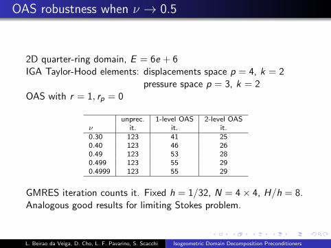
.. OAS robustness when ν → 0.5
2D quarter-ring domain, E = 6e + 6IGA Taylor-Hood elements: displacements space p = 4, k = 2
pressure space p = 3, k = 2OAS with r = 1, rp = 0
unprec. 1-level OAS 2-level OASν it. it. it.0.30 123 41 250.40 123 46 260.49 123 53 280.499 123 55 290.4999 123 55 29
GMRES iteration counts it. Fixed h = 1/32, N = 4× 4, H/h = 8.Analogous good results for limiting Stokes problem.
L. Beirao da Veiga, D. Cho, L. F. Pavarino, S. Scacchi Isogeometric Domain Decomposition Preconditioners
. . . . . .
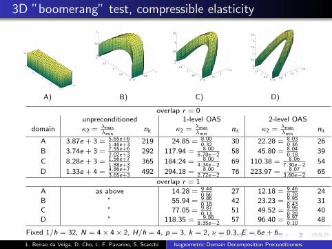
.. 3D ”boomerang” test, compressible elasticity
0
0.5
0
0.5
1
1.5
20
0.5
0
0.5
1
0
0.5
1
1.5
20
0.5
1
0
0.5
1
1.5
0
0.5
1
1.5
20
0.5
1
1.5
00.5
11.5
22.5
00.5
11.5
20
0.5
1
1.5
2
2.5
A) B) C) D)
overlap r = 0unpreconditioned 1-level OAS 2-level OAS
domain κ2 = λmaxλmin
nit κ2 = λmaxλmin
nit κ2 = λmaxλmin
nit
A 3.87e + 3 = 5.65e+61.46e+3
219 24.85 = 8.000.32
30 22.28 = 8.030.36
26
B 3.74e + 3 = 7.55e+62.02e+3
292 117.94 = 8.006.78e−2
58 45.80 = 8.040.18
39
C 8.28e + 3 = 1.56e+71.88e+3
365 184.24 = 8.004.34e−2
69 110.38 = 8.067.30e−2
54
D 1.33e + 4 = 4.86e+73.65e+3
492 294.18 = 8.002.72e−2
76 223.97 = 8.073.60e−2
65
overlap r = 1
A as above 14.28 = 9.440.66
27 12.18 = 9.460.78
24
B ” 55.94 = 9.860.18
42 23.23 = 9.950.43
31
C ” 77.05 = 9.870.13
51 49.52 = 9.960.20
40
D ” 118.35 = 9.888.35e−2
57 96.40 = 9.970.10
48
Fixed 1/h = 32, N = 4× 4× 2, H/h = 4, p = 3, k = 2, ν = 0.3, E = 6e + 6.
L. Beirao da Veiga, D. Cho, L. F. Pavarino, S. Scacchi Isogeometric Domain Decomposition Preconditioners
. . . . . .
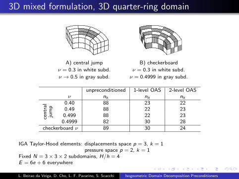
.. 3D mixed formulation, 3D quarter-ring domain
A) central jump B) checkerboard
ν = 0.3 in white subd. ν = 0.3 in white subd.
ν → 0.5 in gray subd. ν = 0.4999 in gray subd.
unpreconditioned 1-level OAS 2-level OASν nit nit nit
central
jump
0.40 88 23 220.49 88 22 230.499 88 22 230.4999 82 30 28
checkerboard ν 89 30 24
IGA Taylor-Hood elements: displacements space p = 3, k = 1pressure space p = 2, k = 1
Fixed N = 3× 3× 2 subdomains, H/h = 4E = 6e + 6 everywhere
L. Beirao da Veiga, D. Cho, L. F. Pavarino, S. Scacchi Isogeometric Domain Decomposition Preconditioners
. . . . . .
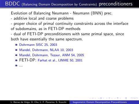
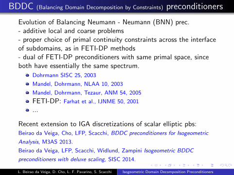
.. BDDC (Balancing Domain Decomposition by Constraints) preconditioners
Evolution of Balancing Neumann - Neumann (BNN) prec.- additive local and coarse problems- proper choice of primal continuity constraints across the interfaceof subdomains, as in FETI-DP methods- dual of FETI-DP preconditioners with same primal space, sinceboth have essentially the same spectrum.
Dohrmann SISC 25, 2003
Mandel, Dohrmann, NLAA 10, 2003
Mandel, Dohrmann, Tezaur, ANM 54, 2005
FETI-DP: Farhat et al., IJNME 50, 2001
...
Recent extension to IGA discretizations of scalar elliptic pbs:Beirao da Veiga, Cho, LFP, Scacchi, BDDC preconditioners for Isogeometric
Analysis, M3AS 2013.
Beirao da Veiga, LFP, Scacchi, Widlund, Zampini Isogeometric BDDC
preconditioners with deluxe scaling, SISC 2014.
L. Beirao da Veiga, D. Cho, L. F. Pavarino, S. Scacchi Isogeometric Domain Decomposition Preconditioners
. . . . . .
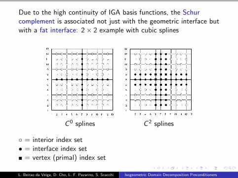
Due to the high continuity of IGA basis functions, the Schurcomplement is associated not just with the geometric interface butwith a fat interface: 2× 2 example with cubic splines
C 0 splines C 2 splines
= interior index set• = interface index set = vertex (primal) index set
L. Beirao da Veiga, D. Cho, L. F. Pavarino, S. Scacchi Isogeometric Domain Decomposition Preconditioners
. . . . . .
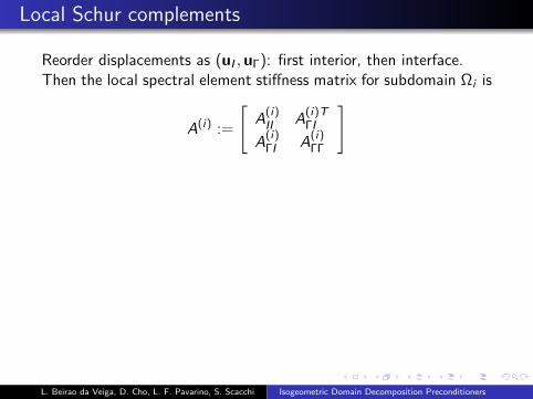
.. Local Schur complements
Reorder displacements as (uI ,uΓ): first interior, then interface.Then the local spectral element stiffness matrix for subdomain Ωi is
A(i) :=
[A(i)II A
(i)TΓI
A(i)ΓI A
(i)ΓΓ
]
Eliminate interior displacements to obtain local Schur complements
S(i)Γ := A
(i)ΓΓ − A
(i)ΓI A
(i)−1II A
(i)TΓI
(only implicit elimination, as Schur complements are not needed,only their action on a vector)Classical Schur complement:
SΓ :=N∑i=1
R(i)T
Γ S(i)Γ R
(i)Γ
L. Beirao da Veiga, D. Cho, L. F. Pavarino, S. Scacchi Isogeometric Domain Decomposition Preconditioners
. . . . . .
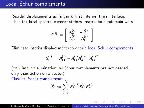
.. Local Schur complements
Reorder displacements as (uI ,uΓ): first interior, then interface.Then the local spectral element stiffness matrix for subdomain Ωi is
A(i) :=
[A(i)II A
(i)TΓI
A(i)ΓI A
(i)ΓΓ
]
Eliminate interior displacements to obtain local Schur complements
S(i)Γ := A
(i)ΓΓ − A
(i)ΓI A
(i)−1II A
(i)TΓI
(only implicit elimination, as Schur complements are not needed,only their action on a vector)Classical Schur complement:
SΓ :=N∑i=1
R(i)T
Γ S(i)Γ R
(i)Γ
L. Beirao da Veiga, D. Cho, L. F. Pavarino, S. Scacchi Isogeometric Domain Decomposition Preconditioners

. . . . . .
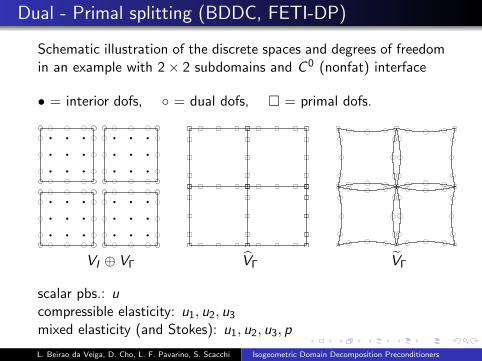
.. Dual - Primal splitting (BDDC, FETI-DP)
Schematic illustration of the discrete spaces and degrees of freedomin an example with 2× 2 subdomains and C 0 (nonfat) interface
• = interior dofs, = dual dofs, = primal dofs.
VI ⊕ VΓ VΓ VΓ
scalar pbs.: ucompressible elasticity: u1, u2, u3mixed elasticity (and Stokes): u1, u2, u3, p
L. Beirao da Veiga, D. Cho, L. F. Pavarino, S. Scacchi Isogeometric Domain Decomposition Preconditioners
. . . . . .
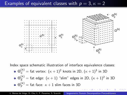
.. Examples of equivalent classes with p = 3, κ = 2
Θ(k)C
Ω(k) Θ(k)E
Θ(k)F
Θ(k)E
Θ(k)C
Ω(k)
Index space schematic illustration of interface equivalence classes:
Θ(k)C = fat vertex: (κ+ 1)2 knots in 2D, (κ+ 1)3 in 3D
Θ(k)E = fat edge: (κ+ 1) “slim” edges in 2D, (κ+ 1)2 in 3D
Θ(k)F = fat face: κ+ 1 slim faces in 3D
L. Beirao da Veiga, D. Cho, L. F. Pavarino, S. Scacchi Isogeometric Domain Decomposition Preconditioners
. . . . . .
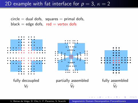
.. 2D example with fat interface for p = 3, κ = 2
circle = dual dofs, squares = primal dofs,black = edge dofs, red = vertex dofs
fully decoupled partially assembled fully assembled
VΓ VΓ VΓ
L. Beirao da Veiga, D. Cho, L. F. Pavarino, S. Scacchi Isogeometric Domain Decomposition Preconditioners
. . . . . .
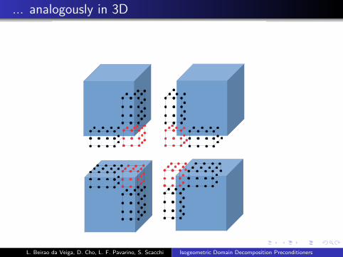
.. ... analogously in 3D
· · ·
fully decoupled edge and vertex equivalence classes
L. Beirao da Veiga, D. Cho, L. F. Pavarino, S. Scacchi Isogeometric Domain Decomposition Preconditioners
. . . . . .
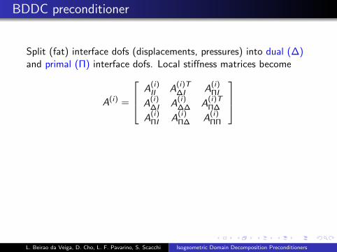
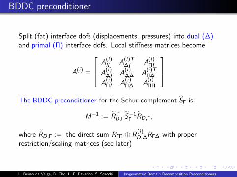
.. BDDC preconditioner
Split (fat) interface dofs (displacements, pressures) into dual (∆)and primal (Π) interface dofs. Local stiffness matrices become
A(i) =
A(i)II A
(i)T∆I A
(i)ΠI
A(i)∆I A
(i)∆∆ A
(i)TΠ∆
A(i)ΠI A
(i)Π∆ A
(i)ΠΠ
The BDDC preconditioner for the Schur complement SΓ is:
M−1 := RTD,ΓS
−1Γ RD,Γ,
where RD,Γ := the direct sum RΓΠ ⊕ R(i)D,∆RΓ∆ with proper
restriction/scaling matrices (see later)
L. Beirao da Veiga, D. Cho, L. F. Pavarino, S. Scacchi Isogeometric Domain Decomposition Preconditioners
. . . . . .
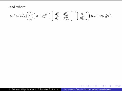
and where
S−1Γ := RT
Γ∆
(N∑i=1
[0 R
(i)T
∆
] [A
(i)II A
(i)T
∆I
A(i)∆I A
(i)∆∆
]−1 [0
R(i)∆
])RΓ∆ +ΦS−1
ΠΠΦT .
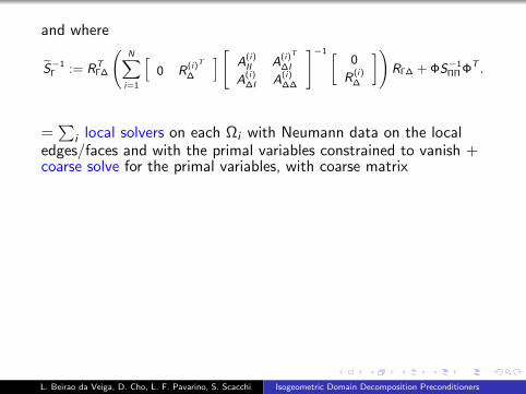
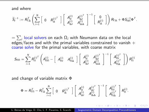
=∑
i local solvers on each Ωi with Neumann data on the localedges/faces and with the primal variables constrained to vanish +coarse solve for the primal variables, with coarse matrix
SΠΠ =N∑i=1
R(i)T
Π
(A
(i)ΠΠ −
[A
(i)ΠI A
(i)Π∆
] [A
(i)II A
(i)T
∆I
A(i)∆I A
(i)∆∆
]−1 [A
(i)T
ΠI
A(i)T
Π∆
])R
(i)Π
and change of variable matrix Φ
Φ = RTΓΠ − RT
Γ∆
N∑i=1
[0 R
(i)T
∆
] [A
(i)II A
(i)T
∆I
A(i)∆I A
(i)∆∆
]−1 [A
(i)T
ΠI
A(i)T
Π∆
]R
(i)Π .
L. Beirao da Veiga, D. Cho, L. F. Pavarino, S. Scacchi Isogeometric Domain Decomposition Preconditioners
. . . . . .
and where
S−1Γ := RT
Γ∆
(N∑i=1
[0 R
(i)T
∆
] [A
(i)II A
(i)T
∆I
A(i)∆I A
(i)∆∆
]−1 [0
R(i)∆
])RΓ∆ +ΦS−1
ΠΠΦT .
=∑
i local solvers on each Ωi with Neumann data on the localedges/faces and with the primal variables constrained to vanish +coarse solve for the primal variables, with coarse matrix
SΠΠ =N∑i=1
R(i)T
Π
(A
(i)ΠΠ −
[A
(i)ΠI A
(i)Π∆
] [A
(i)II A
(i)T
∆I
A(i)∆I A
(i)∆∆
]−1 [A
(i)T
ΠI
A(i)T
Π∆
])R
(i)Π
and change of variable matrix Φ
Φ = RTΓΠ − RT
Γ∆
N∑i=1
[0 R
(i)T
∆
] [A
(i)II A
(i)T
∆I
A(i)∆I A
(i)∆∆
]−1 [A
(i)T
ΠI
A(i)T
Π∆
]R
(i)Π .
L. Beirao da Veiga, D. Cho, L. F. Pavarino, S. Scacchi Isogeometric Domain Decomposition Preconditioners
. . . . . .
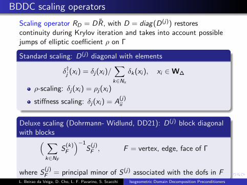
.. BDDC scaling operators
Scaling operator RD = DR, with D = diag(D(j)) restorescontinuity during Krylov iteration and takes into account possiblejumps of elliptic coefficient ρ on Γ.Standard scaling: D(j) diagonal with elements..
......
δ†j (xi ) = δj(xi )/∑k∈Nx
δk(xi ), xi ∈ W∆
ρ-scaling: δj(xi ) = ρj(xi )
stiffness scaling: δj(xi ) = A(j)ii
.Deluxe scaling (Dohrmann- Widlund, DD21): D(j) block diagonalwith blocks..
......
( ∑k∈NF
S(k)F
)−1S(j)F , F = vertex, edge, face of Γ
where S(j)F = principal minor of S (j) associated with the dofs in F
L. Beirao da Veiga, D. Cho, L. F. Pavarino, S. Scacchi Isogeometric Domain Decomposition Preconditioners
. . . . . .
.. Possible choices of primal constraints
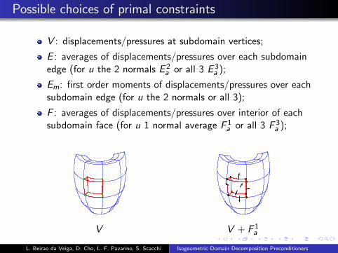
V : displacements/pressures at subdomain vertices;
E : averages of displacements/pressures over each subdomainedge (for u the 2 normals E 2
a or all 3 E 3a );
Em: first order moments of displacements/pressures over eachsubdomain edge (for u the 2 normals or all 3);
F : averages of displacements/pressures over interior of eachsubdomain face (for u 1 normal average F 1
a or all 3 F 3a );
V V + F 1a
L. Beirao da Veiga, D. Cho, L. F. Pavarino, S. Scacchi Isogeometric Domain Decomposition Preconditioners
. . . . . .
.. Possible choices of primal constraints
V : displacements/pressures at subdomain vertices;
E : averages of displacements/pressures over each subdomainedge (for u the 2 normals E 2
a or all 3 E 3a );
Em: first order moments of displacements/pressures over eachsubdomain edge (for u the 2 normals or all 3);
F : averages of displacements/pressures over interior of eachsubdomain face (for u 1 normal average F 1
a or all 3 F 3a );
V V + F 1a
L. Beirao da Veiga, D. Cho, L. F. Pavarino, S. Scacchi Isogeometric Domain Decomposition Preconditioners
. . . . . .
.. IGA BDDC convergence rate bounds for elliptic pbs.
.Theorem..
......
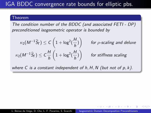
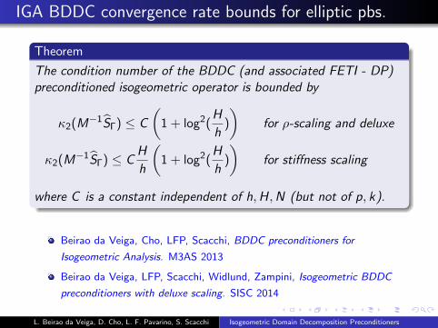
The condition number of the BDDC (and associated FETI - DP)preconditioned isogeometric operator is bounded by
κ2(M−1SΓ) ≤ C
(1 + log2(
H
h)
)for ρ-scaling and deluxe
κ2(M−1SΓ) ≤ C
H
h
(1 + log2(
H
h)
)for stiffness scaling
where C is a constant independent of h,H,N (but not of p, k).
Beirao da Veiga, Cho, LFP, Scacchi, BDDC preconditioners for
Isogeometric Analysis. M3AS 2013
Beirao da Veiga, LFP, Scacchi, Widlund, Zampini, Isogeometric BDDC
preconditioners with deluxe scaling. SISC 2014
L. Beirao da Veiga, D. Cho, L. F. Pavarino, S. Scacchi Isogeometric Domain Decomposition Preconditioners
. . . . . .
.. IGA BDDC convergence rate bounds for elliptic pbs.
.Theorem..
......
The condition number of the BDDC (and associated FETI - DP)preconditioned isogeometric operator is bounded by
κ2(M−1SΓ) ≤ C
(1 + log2(
H
h)
)for ρ-scaling and deluxe
κ2(M−1SΓ) ≤ C
H
h
(1 + log2(
H
h)
)for stiffness scaling
where C is a constant independent of h,H,N (but not of p, k).
Beirao da Veiga, Cho, LFP, Scacchi, BDDC preconditioners for
Isogeometric Analysis. M3AS 2013
Beirao da Veiga, LFP, Scacchi, Widlund, Zampini, Isogeometric BDDC
preconditioners with deluxe scaling. SISC 2014
L. Beirao da Veiga, D. Cho, L. F. Pavarino, S. Scacchi Isogeometric Domain Decomposition Preconditioners
. . . . . .
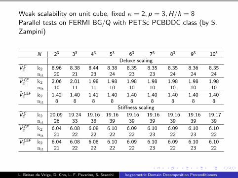
Weak scalability on unit cube, fixed κ = 2, p = 3,H/h = 8Parallel tests on FERMI BG/Q with PETSc PCBDDC class (by S.Zampini)
N 23 33 43 53 63 73 83 93 103
Deluxe scaling
V CΠ k2 8.96 8.38 8.44 8.38 8.35 8.35 8.35 8.36 8.35
nit 20 21 23 24 23 23 24 24 24
V CEΠ k2 2.06 2.01 1.98 1.98 1.98 1.98 1.98 1.98 1.98
nit 10 11 11 10 10 10 10 10 10
V CEFΠ k2 1.42 1.40 1.41 1.40 1.40 1.40 1.40 1.40 1.40
nit 8 8 8 8 8 8 8 8 8Stiffness scaling
V CΠ k2 20.09 19.24 19.16 19.16 19.16 19.16 19.16 19.16 19.17
nit 26 33 38 39 39 39 39 39 39
V CEΠ k2 6.04 6.08 6.08 6.10 6.09 6.10 6.09 6.10 6.10
nit 21 22 22 22 22 23 22 23 22
V CEFΠ k2 6.04 6.08 6.08 6.10 6.09 6.10 6.09 6.10 6.10
nit 21 22 22 22 22 23 22 23 22
L. Beirao da Veiga, D. Cho, L. F. Pavarino, S. Scacchi Isogeometric Domain Decomposition Preconditioners
. . . . . .
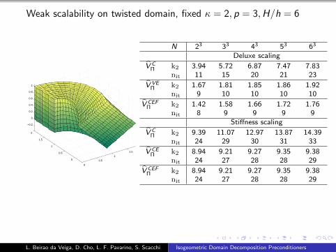
Weak scalability on twisted domain, fixed κ = 2, p = 3,H/h = 6
0
0.5
1
1.5
0
0.5
1
1.5
2
−0.2
0
0.2
0.4
0.6
0.8
1
N 23 33 43 53 63
Deluxe scaling
V CΠ k2 3.94 5.72 6.87 7.47 7.83
nit 11 15 20 21 23
V VEΠ k2 1.67 1.81 1.85 1.86 1.92
nit 9 10 10 10 10
V CEFΠ k2 1.42 1.58 1.66 1.72 1.76
nit 8 9 9 9 9Stiffness scaling
V CΠ k2 9.39 11.07 12.97 13.87 14.39
nit 24 29 30 31 33
V CEΠ k2 8.94 9.21 9.27 9.35 9.38
nit 24 27 28 28 29
V CEFΠ k2 8.94 9.21 9.27 9.35 9.38
nit 24 27 28 28 29
L. Beirao da Veiga, D. Cho, L. F. Pavarino, S. Scacchi Isogeometric Domain Decomposition Preconditioners

. . . . . .
BDDC deluxe robustness with respect to jump discontinuities inthe diffusion coefficient ρ,fixed h = 1/32, p = 3, C 0 continuity at the interface, 4× 4× 4subdomains
central jump checkerboard random mixρ k2 nit k2 nit k2 nit
10−4 117.37 44 — — — —10−2 118.40 44 — — — —
V CΠ 1 134.04 48 134.04 48 134.04 48
102 137.15 50 102.11 43 126.53 47104 137.40 52 104.31 44 123.63 4610−4 5.33 18 — — — —10−2 5.33 18 — — — —
V CEΠ 1 5.27 18 5.27 18 5.27 18
102 4.92 16 4.19 16 4.83 16104 4.88 16 4.20 16 4.87 1610−4 1.98 10 1.98 10 — —10−2 1.99 10 1.99 10 — —
V CEFΠ 1 2.05 10 2.05 10 2.05 10
102 2.05 10 2.05 10 2.00 10104 2.05 10 2.05 10 2.00 9
L. Beirao da Veiga, D. Cho, L. F. Pavarino, S. Scacchi Isogeometric Domain Decomposition Preconditioners
. . . . . .
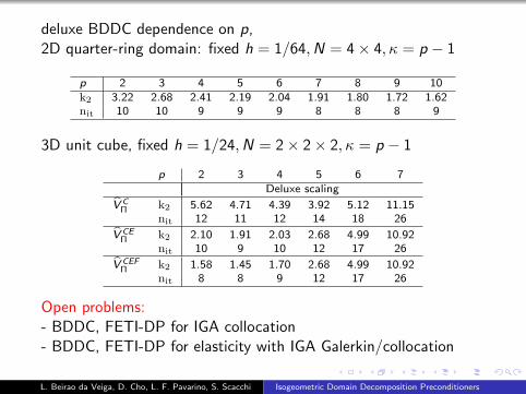
deluxe BDDC dependence on p,2D quarter-ring domain: fixed h = 1/64,N = 4× 4, κ = p − 1
p 2 3 4 5 6 7 8 9 10k2 3.22 2.68 2.41 2.19 2.04 1.91 1.80 1.72 1.62nit 10 10 9 9 9 8 8 8 9
3D unit cube, fixed h = 1/24,N = 2× 2× 2, κ = p − 1
p 2 3 4 5 6 7Deluxe scaling
V CΠ k2 5.62 4.71 4.39 3.92 5.12 11.15
nit 12 11 12 14 18 26
V CEΠ k2 2.10 1.91 2.03 2.68 4.99 10.92
nit 10 9 10 12 17 26
V CEFΠ k2 1.58 1.45 1.70 2.68 4.99 10.92
nit 8 8 9 12 17 26
Open problems:- BDDC, FETI-DP for IGA collocation- BDDC, FETI-DP for elasticity with IGA Galerkin/collocation
L. Beirao da Veiga, D. Cho, L. F. Pavarino, S. Scacchi Isogeometric Domain Decomposition Preconditioners
. . . . . .
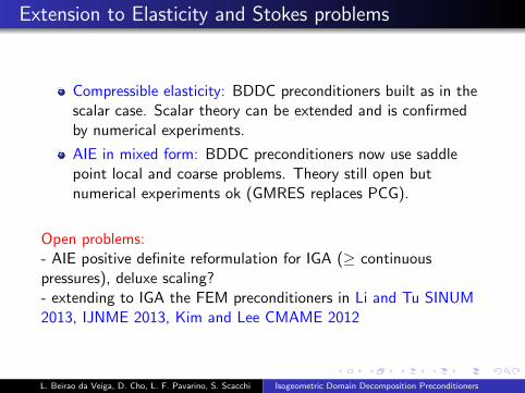
.. Extension to Elasticity and Stokes problems
Compressible elasticity: BDDC preconditioners built as in thescalar case. Scalar theory can be extended and is confirmedby numerical experiments.
AIE in mixed form: BDDC preconditioners now use saddlepoint local and coarse problems. Theory still open butnumerical experiments ok (GMRES replaces PCG).
Open problems:- AIE positive definite reformulation for IGA (≥ continuouspressures), deluxe scaling?- extending to IGA the FEM preconditioners in Li and Tu SINUM2013, IJNME 2013, Kim and Lee CMAME 2012
L. Beirao da Veiga, D. Cho, L. F. Pavarino, S. Scacchi Isogeometric Domain Decomposition Preconditioners
. . . . . .
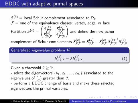
.. BDDC with adaptive primal spaces
S (k) = local Schur complement associated to Ωk
F = one of the equivalence classes: vertex, edge, or face
Partition S (k) =
(S(k)FF S
(k)FF ′
S(k)F ′F S
(k)F ′F ′
)and define the new Schur
complement of Schur complements S(k)FF = S
(k)FF − S
(k)FF ′S
(k)−1
F ′F ′ S(k)F ′F
.Generalized eigenvalue problem V1..
...... S(k)FFv = λS
(k)FFv . (1)
Given a threshold θ ≥ 1:- select the eigenvectors v1, v2, . . . , vNc associated to theeigenvalues of (1) greater than θ,- perform a BDDC change of basis and make these selectedeigenvectors the primal variables.
L. Beirao da Veiga, D. Cho, L. F. Pavarino, S. Scacchi Isogeometric Domain Decomposition Preconditioners
. . . . . .
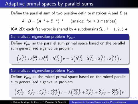
.. Adaptive primal spaces by parallel sums
Define the parallel sum of two positive definite matrices A and B as
A : B = (A−1 + B−1)−1 (analog. for ≥ 3 matrices)
IGA 2D: each fat vertex is shared by 4 subdomains Ωi , i = 1, 2, 3, 4.Generalized eigenvalue problem Vpar :..
......
Define Vpar as the parallel sum primal space based on the parallelsum generalized eigenvalue problem(
S(1)FF : S
(2)FF : S
(3)FF : S
(4)FF
)v = λ
(S(1)FF : S
(2)FF : S
(3)FF : S
(4)FF
)v
.Generalized eigenvalue problem Vmix :..
......
Define Vmix as the mixed primal space based on the mixed parallelsum generalized eigenvalue problem(
S(1)FF : S
(2)FF : S
(3)FF : S
(4)FF
)v = λ
(S(1)FF + S
(2)FF + S
(3)FF + S
(4)FF
)v
L. Beirao da Veiga, D. Cho, L. F. Pavarino, S. Scacchi Isogeometric Domain Decomposition Preconditioners
. . . . . .
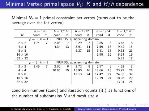
.. Minimal Vertex primal space V1: K and H/h dependence
Minimal Nc = 1 primal constraint per vertex (turns out to be theaverage over the fat vertex)
h = 1/8 h = 1/16 h = 1/32 h = 1/64 h = 1/128N cond it. cond it. cond it. cond it. cond it.
p = 3, k = 1 NURBS, quarter-ring domain2× 2 1.74 7 2.08 7 2.29 7 2.85 8 3.45 84× 4 4.34 13 5.91 14 7.59 15 9.42 158× 8 5.37 15 7.41 18 9.53 21
16× 16 5.98 16 8.34 1932× 32 6.31 17
p = 3, k = 2 NURBS, quarter-ring domain2× 2 1.45 7 2.00 8 2.72 8 3.57 8 4.52 84× 4 10.06 15 13.90 16 18.66 18 23.92 218× 8 12.13 24 17.42 27 24.85 32
16× 16 12.79 24 18.96 2932× 32 13.04 24
condition number (cond) and iteration counts (it.) as functions ofthe number of subdomains N and mesh size h.
L. Beirao da Veiga, D. Cho, L. F. Pavarino, S. Scacchi Isogeometric Domain Decomposition Preconditioners
. . . . . .
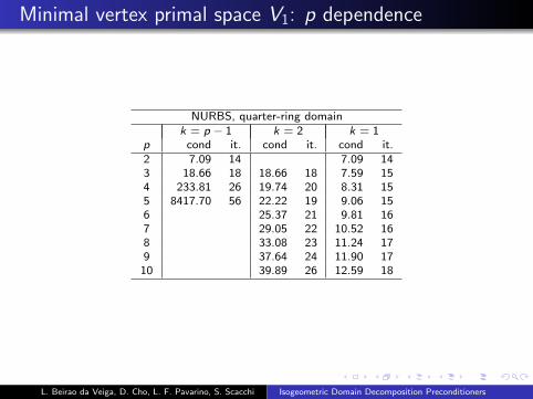
.. Minimal vertex primal space V1: p dependence
NURBS, quarter-ring domaink = p − 1 k = 2 k = 1
p cond it. cond it. cond it.2 7.09 14 7.09 143 18.66 18 18.66 18 7.59 154 233.81 26 19.74 20 8.31 155 8417.70 56 22.22 19 9.06 156 25.37 21 9.81 167 29.05 22 10.52 168 33.08 23 11.24 179 37.64 24 11.90 1710 39.89 26 12.59 18
L. Beirao da Veiga, D. Cho, L. F. Pavarino, S. Scacchi Isogeometric Domain Decomposition Preconditioners
. . . . . .
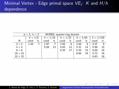
..
Minimal Vertex - Edge primal space VE1: K and H/hdependence
p = 3, k = 2 NURBS, quarter-ring domainh = 1/8 h = 1/16 h = 1/32 h = 1/64 h = 1/128
N cond it. cond it. cond it. cond it. cond it.2× 2 1.44 7 1.97 7 2.65 8 3.46 8 4.37 84× 4 5.09 13 4.65 13 5.31 14 5.99 158× 8 6.20 17 5.34 15 6.00 16
16× 16 6.66 18 5.73 1632× 32 6.83 18
L. Beirao da Veiga, D. Cho, L. F. Pavarino, S. Scacchi Isogeometric Domain Decomposition Preconditioners

. . . . . .
.. Minimal Vertex - Edge primal space VE1: p dependence
Minimal Nc = 1 primal constraint per vertex and Nc = 1 per edge
NURBS, quarter-ring domaink = p − 1 k = 2 k = 1
p cond it. cond it. cond it.2 2.91 11 2.91 113 5.31 14 5.31 14 2.80 114 41.17 24 4.85 21 2.88 115 1598.65 67 4.77 14 3.00 116 4.93 15 3.13 117 5.16 16 3.27 128 5.67 17 3.40 129 3.53 1310 3.71 13
L. Beirao da Veiga, D. Cho, L. F. Pavarino, S. Scacchi Isogeometric Domain Decomposition Preconditioners
. . . . . .
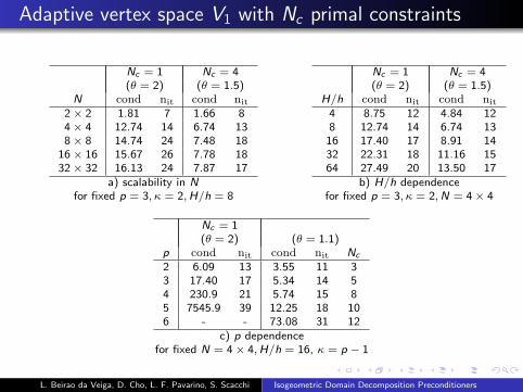
.. Adaptive vertex space V1 with Nc primal constraints
Nc = 1 Nc = 4(θ = 2) (θ = 1.5)
N cond nit cond nit2× 2 1.81 7 1.66 84× 4 12.74 14 6.74 138× 8 14.74 24 7.48 18
16× 16 15.67 26 7.78 1832× 32 16.13 24 7.87 17
Nc = 1 Nc = 4(θ = 2) (θ = 1.5)
H/h cond nit cond nit4 8.75 12 4.84 128 12.74 14 6.74 1316 17.40 17 8.91 1432 22.31 18 11.16 1564 27.49 20 13.50 17
a) scalability in N b) H/h dependencefor fixed p = 3, κ = 2,H/h = 8 for fixed p = 3, κ = 2,N = 4× 4
Nc = 1(θ = 2) (θ = 1.1)
p cond nit cond nit Nc
2 6.09 13 3.55 11 33 17.40 17 5.34 14 54 230.9 21 5.74 15 85 7545.9 39 12.25 18 106 - - 73.08 31 12
c) p dependencefor fixed N = 4× 4,H/h = 16, κ = p − 1
L. Beirao da Veiga, D. Cho, L. F. Pavarino, S. Scacchi Isogeometric Domain Decomposition Preconditioners
. . . . . .
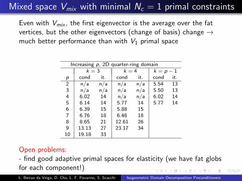
.. Mixed space Vmix with minimal Nc = 1 primal constraints
Even with Vmix , the first eigenvector is the average over the fatvertices, but the other eigenvectors (change of basis) change →much better performance than with V1 primal space
Increasing p, 2D quarter-ring domaink = 3 k = 4 k = p − 1
p cond it. cond it. cond it.2 n/a n/a n/a n/a 5.54 133 n/a n/a n/a n/a 5.50 134 6.02 14 n/a n/a 6.02 145 6.14 14 5.77 14 5.77 146 6.39 15 5.88 157 6.76 18 6.48 188 8.65 21 12.61 269 13.13 27 23.17 3410 19.18 33
Open problems:- find good adaptive primal spaces for elasticity (we have fat globsfor each component!)L. Beirao da Veiga, D. Cho, L. F. Pavarino, S. Scacchi Isogeometric Domain Decomposition Preconditioners
. . . . . .
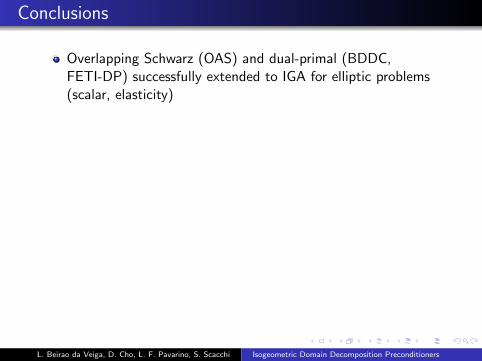
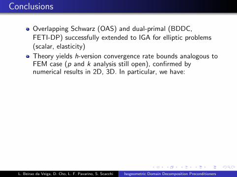
.. Conclusions
Overlapping Schwarz (OAS) and dual-primal (BDDC,FETI-DP) successfully extended to IGA for elliptic problems(scalar, elasticity)
Theory yields h-version convergence rate bounds analogous toFEM case (p and k analysis still open), confirmed bynumerical results in 2D, 3D. In particular, we have:
parallel scalabilityH/h - optimality (OAS), H/h - quasi-optimality (BDDC)robustness with respect to discontinuous elliptic coefficientsOAS: robustness in p (indep. for generous overlap) and kdeluxe BDDC very efficient for IGA fat interfaces, adaptiveprimal choices available
Future work: dual-primal methods for elasticity and Stokesproblems, IGA collocation, DD for IGA adaptivity (T-splines,LR splines, etc.)
THANK YOU
L. Beirao da Veiga, D. Cho, L. F. Pavarino, S. Scacchi Isogeometric Domain Decomposition Preconditioners
. . . . . .
.. Conclusions
Overlapping Schwarz (OAS) and dual-primal (BDDC,FETI-DP) successfully extended to IGA for elliptic problems(scalar, elasticity)
Theory yields h-version convergence rate bounds analogous toFEM case (p and k analysis still open), confirmed bynumerical results in 2D, 3D. In particular, we have:
parallel scalabilityH/h - optimality (OAS), H/h - quasi-optimality (BDDC)robustness with respect to discontinuous elliptic coefficientsOAS: robustness in p (indep. for generous overlap) and kdeluxe BDDC very efficient for IGA fat interfaces, adaptiveprimal choices available
Future work: dual-primal methods for elasticity and Stokesproblems, IGA collocation, DD for IGA adaptivity (T-splines,LR splines, etc.)
THANK YOU
L. Beirao da Veiga, D. Cho, L. F. Pavarino, S. Scacchi Isogeometric Domain Decomposition Preconditioners
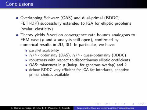
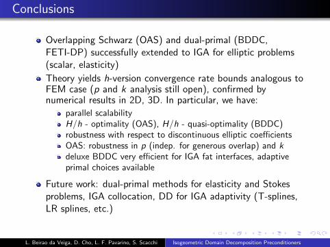
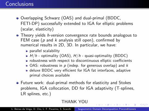


![Robust domain decomposition preconditioners for abstract ... · In this paper, we extend the frameworkproposed in [10,11] to general symmetric bilinear forms. The resulting analysis](https://img.pdfslide.us/doc/110x75/5f5b0999e493cf688b3706db/robust-domain-decomposition-preconditioners-for-abstract-in-this-paper-we-extend.jpg)