COMPATIBLE DISCRETIZATIONS FOR MAXWELL EQUATIONS · COMPATIBLE DISCRETIZATIONS FOR MAXWELL EQUATIONS ... systematic way to derive stable local ﬂnite-diﬁerence stencils ... \Less

$Page 1: COMPATIBLE DISCRETIZATIONS FOR MAXWELL EQUATIONS · COMPATIBLE DISCRETIZATIONS FOR MAXWELL EQUATIONS ... systematic way to derive stable local ﬂnite-diﬁerence stencils ... \Less$
COMPATIBLE DISCRETIZATIONS FOR MAXWELL

EQUATIONS

DISSERTATION

Presented in Partial Fulfillment of the Requirements for

the Degree Doctor of Philosophy in the

Graduate School of The Ohio State University

By

Bo He, B.S., M.S., Ph.D.

* * * * *

The Ohio State University

2006

Dissertation Committee:

Professor Fernando Teixeira, Adviser

Professor Robert Lee

Professor Prabhakar Pathak

Approved by

Adviser

Graduate Program inElectrical and Computer

Engineering

c© Copyright by

Bo He

2006

ABSTRACT

The main focus of this dissertation is the study and development of numerical

techniques to solve Maxwell equations on irregular lattices. This is achieved by means

of compatible discretizations that rely on some tools of algebraic topology and a

discrete analog of differential forms on a lattice.

Using discrete Hodge decomposition and Euler’s formula for a network of polyhe-

dra, we show that the number of dynamic degrees of freedom (DoFs) of the electric

field equals the number of dynamic DoFs of the magnetic field on an arbitrary lat-

tice (cell complex). This identity reflects an essential property of discrete Maxwell

equations (Hamiltonian structure) that any compatible discretization scheme should

observe. We unveil a new duality called Galerkin duality, a transformation between

two (discrete) systems, primal system and dual system. If the discrete Hodge oper-

ators are realized by Galerkin Hodges, we show that the primal system recovers the

conventional edge-element FEM and suggests a geometric foundation for it. On the

other hand, the dual system suggests a new (dual) type of FEM.

We find that inverse Hodge matrices have strong localization properties. Hence

we propose two thresholding techniques, viz., algebraic thresholding and topological

thresholding, to sparsify inverse Hodge matrices. Based on topological thresholding,

we propose a sparse and fully explicit time-domain FEM for Maxwell equations.

ii

From a finite-difference viewpoint, topological thresholding provides a general and

systematic way to derive stable local finite-difference stencils in irregular grids.

We also propose and implement an E-B mixed FEM scheme to discretize first

order Maxwell equations in frequency domain directly. This scheme results in sparse

matrices.

In order to tackle low-frequency instabilities in frequency domain FEM and spuri-

ous linear growth of time domain FEM solutions, we propose some gauging techniques

to regularize the null space of a curl operator.

iii

This work is dedicated to my wife Xueqin.

iv

ACKNOWLEDGMENTS

First and foremost, I would like to thank my adviser, Professor Fernando Teixeira

for his invaluable guidance, encouragement and support.

I would also like to thank my other committee members: Professor Robert Lee

and Professor Prabhakar Pathak, for their helpful discussions and suggestions.

I would like to thank all my courses’ instructors, especially Professor Jin-Fa Lee

and Professor Ben Munk for their stimulating lectures.

Thanks to all my colleagues of ESL lab, especially Yik-Kiong Hue and Guangdong

Pan.

I would like to thank Professor Ta-Pei Cheng (University of Missouri - St. Louis)

for his encouragement and early scientific training.

I am grateful for the constant support and encouragement from my parents and

parents-in-law.

I would like to thank my son Jingyan(Leo) for bringing me happiness.

Last but not least, I would like to thank my wife, Xueqin, without her support,

this work would not have been possible. This work is dedicated to her.

This work was partially supported by NSF under grant ECS-0347502, AFOSR

under grant FA-9550-04-1-0359, and OSC under grants PAS-0061 and PAS-0110.

v

VITA

March 14, 1969 . . . . . . . . . . . . . . . . . . . . . . . . . . . . . Born - Changzhi, P. R. China.

1991 . . . . . . . . . . . . . . . . . . . . . . . . . . . . . . . . . . . . . . . .B.S. Electrical Engineering, ShanxiUniversity.

1994 . . . . . . . . . . . . . . . . . . . . . . . . . . . . . . . . . . . . . . . .M.S. Physics, East China Normal Uni-versity.

1994-1999 . . . . . . . . . . . . . . . . . . . . . . . . . . . . . . . . . . Faculty Member, Shanghai Jiao TongUniversity.

2002 . . . . . . . . . . . . . . . . . . . . . . . . . . . . . . . . . . . . . . . .Ph.D. Physics, University of Missouri,Rolla/St. Louis.

2002-present . . . . . . . . . . . . . . . . . . . . . . . . . . . . . . . .Graduate Research Associate, Electri-cal and Computer Engineering, TheOhio State University.

PUBLICATIONS

Research Publications

B. He and F.L. Teixeira, “A sparse and explicit FETD via approximate inverseHodge (mass) matrix,” accepted by IEEE Microwave and Wireless Components Let-ters.

B. He and F.L. Teixeira, “An E-B mixed FEM for first-order Maxwell curl equa-tions,” accepted by 12th Biennial IEEE Conference on Electromagnetic Field Com-putation, Miami, 2006.

B. He and F.L. Teixeira, “Geometric finite element discretization of Maxwellequations in primal and dual spaces,” Phys. Lett. A 349, 1-14, 2006.

vi

B. He and F.L. Teixeira, “On the degrees of freedom of lattice electrodynamics,”Phys. Lett. A 336, 1-7, 2005.

B. He and F.L. Teixeira, “Compatible discretizations of Maxwell equations,”AP/URSI 2005, Washington, DC, July, 2005.

B. He and F.L. Teixeira, “Gauging in discrete solution spaces of the wave equa-tions,” AP/URSI 2005, Washington, DC, July, 2005.

B. He and F.L. Teixeira, “Primal and dual spaces in the FEM solution of Maxwellequations,” SIAM Conference on Computational Science and Engineering Program,Orlando, FL, February, 2005.

B. He and F.L. Teixeira, “Discrete Helmholtz decomposition, Euler’s formula, andthe degrees of freedom of lattice electrodynamics,” AP/URSI 2004, Monterey, CA,June, 2004.

F.L. Teixeira and B. He, “On grid subdivisions for the simplicial discretization ofMaxwell’s equations,” AP/URSI 2003, Columbus, OH, June 2003.

Selected Research Publications in Physics

B. He, T.P. Cheng, and L.F. Li, “Less suppressed µ → eγ and τ → µγ loopamplitudes and extra dimension theories,” Phys. Lett. B 553, 277-283, 2003.

W. Zhu, K.M. Chai, and B. He, “Predictions for the low-x structure function inthe modified GLR equation,” Nucl. Phys. B 449, 183-196, 1995.

W. Zhu, K.M. Chai, and B. He, “Antishadowing properties in the small-x region,”Nucl. Phys. B 427, 525-533, 1994.

FIELDS OF STUDY

Major Field: Electrical Engineering

vii

TABLE OF CONTENTS

Page

Abstract . . . . . . . . . . . . . . . . . . . . . . . . . . . . . . . . . . . . . . . ii

Dedication . . . . . . . . . . . . . . . . . . . . . . . . . . . . . . . . . . . . . . iv

Acknowledgments . . . . . . . . . . . . . . . . . . . . . . . . . . . . . . . . . . v

Vita . . . . . . . . . . . . . . . . . . . . . . . . . . . . . . . . . . . . . . . . . vi

List of Tables . . . . . . . . . . . . . . . . . . . . . . . . . . . . . . . . . . . . xi

List of Figures . . . . . . . . . . . . . . . . . . . . . . . . . . . . . . . . . . . xiii

Chapters:

1. Introduction . . . . . . . . . . . . . . . . . . . . . . . . . . . . . . . . . . 1

1.1 Background and motivation . . . . . . . . . . . . . . . . . . . . . . 11.2 Organization of this dissertation . . . . . . . . . . . . . . . . . . . 2

2. Mathematical preliminaries . . . . . . . . . . . . . . . . . . . . . . . . . 5

2.1 Differential forms . . . . . . . . . . . . . . . . . . . . . . . . . . . . 52.2 Chains and cochains . . . . . . . . . . . . . . . . . . . . . . . . . . 92.3 Whitney forms . . . . . . . . . . . . . . . . . . . . . . . . . . . . . 16

2.3.1 Recursive (generating) relation . . . . . . . . . . . . . . . . 162.3.2 Local gauging property . . . . . . . . . . . . . . . . . . . . 172.3.3 De Rham diagram (exact sequence property) . . . . . . . . 192.3.4 Whitney elements in local coordinates . . . . . . . . . . . . 19

viii

3. Compatible discretizations for Maxwell equations . . . . . . . . . . . . . 21

3.1 Maxwell equations in differential forms language . . . . . . . . . . . 223.2 Discrete exterior differential operators . . . . . . . . . . . . . . . . 233.3 Discrete Hodge operators . . . . . . . . . . . . . . . . . . . . . . . 29

3.3.1 Yee Hodges . . . . . . . . . . . . . . . . . . . . . . . . . . . 293.3.2 Galerkin Hodges . . . . . . . . . . . . . . . . . . . . . . . . 31

3.4 Additional remarks . . . . . . . . . . . . . . . . . . . . . . . . . . . 32

4. Discrete Hodge decomposition . . . . . . . . . . . . . . . . . . . . . . . . 35

4.1 Discrete Hodge decomposition . . . . . . . . . . . . . . . . . . . . . 354.1.1 2+1 theory in a contractible domain . . . . . . . . . . . . . 364.1.2 3+1 theory in a contractible domain . . . . . . . . . . . . . 374.1.3 2+1 theory in a non-contractible domain . . . . . . . . . . . 394.1.4 Euler’s formula and Hodge decomposition . . . . . . . . . . 404.1.5 Example: Yee lattice . . . . . . . . . . . . . . . . . . . . . . 41

4.2 Some local properties of the discrete Hodge decomposition . . . . . 424.3 Symplectic structure . . . . . . . . . . . . . . . . . . . . . . . . . . 454.4 Additional remarks . . . . . . . . . . . . . . . . . . . . . . . . . . . 46

5. FEM in primal and dual spaces: Galerkin duality . . . . . . . . . . . . . 47

5.1 Primal and dual discrete wave equations . . . . . . . . . . . . . . . 485.2 Stiffness matrices: geometric viewpoint . . . . . . . . . . . . . . . . 50

5.2.1 Triangular element . . . . . . . . . . . . . . . . . . . . . . . 515.2.2 Square element . . . . . . . . . . . . . . . . . . . . . . . . . 52

5.3 Galerkin duality . . . . . . . . . . . . . . . . . . . . . . . . . . . . 545.4 An approach to handle Neumann boundary conditions . . . . . . . 555.5 Galerkin duality: Examples . . . . . . . . . . . . . . . . . . . . . . 55

5.5.1 2D examples and discussion . . . . . . . . . . . . . . . . . . 565.5.2 Discrete Hodge decomposition for 2D . . . . . . . . . . . . . 605.5.3 3D examples and discussion . . . . . . . . . . . . . . . . . . 635.5.4 Discrete Hodge decomposition in 3D . . . . . . . . . . . . . 66

6. Sparse approximation of inverse Hodge (mass) matrices . . . . . . . . . . 68

6.1 Strong localization property . . . . . . . . . . . . . . . . . . . . . . 706.2 Sparse approximate inverse mass matrices . . . . . . . . . . . . . . 70

6.2.1 Algebraic thresholding . . . . . . . . . . . . . . . . . . . . . 716.2.2 Sparsity and sparsification error trade-off . . . . . . . . . . 716.2.3 Topological thresholding . . . . . . . . . . . . . . . . . . . . 75

ix

6.2.4 Connection with SPAI preconditioners . . . . . . . . . . . . 796.3 Explicit sparse FETD . . . . . . . . . . . . . . . . . . . . . . . . . 80

6.3.1 Sparse and explicit FETD via an algebraic-based sparsifica-tion of the inverse mass matrix . . . . . . . . . . . . . . . . 82

6.3.2 Sparse and explicit FETD via a topological-based sparsifica-tion of the inverse mass matrix . . . . . . . . . . . . . . . . 87


7. An E-B mixed finite element method . . . . . . . . . . . . . . . . . . . . 90

7.1 Formulation . . . . . . . . . . . . . . . . . . . . . . . . . . . . . . . 917.2 Numerical examples . . . . . . . . . . . . . . . . . . . . . . . . . . 92

7.2.1 2D circular cavity . . . . . . . . . . . . . . . . . . . . . . . 927.2.2 Spherical cavity . . . . . . . . . . . . . . . . . . . . . . . . . 937.2.3 Zero (static) mode and nonzero (dynamical) mode structure 947.2.4 Band structure of photonic crystals . . . . . . . . . . . . . . 95

8. Gauging in discrete spaces . . . . . . . . . . . . . . . . . . . . . . . . . . 98

8.1 Singularity of the curl operator . . . . . . . . . . . . . . . . . . . . 988.2 Constraint equations . . . . . . . . . . . . . . . . . . . . . . . . . . 998.3 Divergence-free condition . . . . . . . . . . . . . . . . . . . . . . . 100

8.3.1 Electrical field distributions of zero modes and nonzero modes 1008.3.2 Global (discrete) divergence . . . . . . . . . . . . . . . . . . 101

8.4 Global gauging in frequency domain . . . . . . . . . . . . . . . . . 1038.4.1 Global gauging in primal formulation . . . . . . . . . . . . . 1048.4.2 Global gauging in dual formulation . . . . . . . . . . . . . . 106

8.5 Global gauging in time domain . . . . . . . . . . . . . . . . . . . . 1108.5.1 Second order wave equation: FETD solutions . . . . . . . . 1128.5.2 First order wave equations: FETD solutions . . . . . . . . . 116


9. Conclusions . . . . . . . . . . . . . . . . . . . . . . . . . . . . . . . . . . 119

Appendices:

A. Stiffness matrices: geometric viewpoint . . . . . . . . . . . . . . . . . . . 122

A.1 Tetrahedral element . . . . . . . . . . . . . . . . . . . . . . . . . . 122A.2 Cubic element . . . . . . . . . . . . . . . . . . . . . . . . . . . . . 124

Bibliography . . . . . . . . . . . . . . . . . . . . . . . . . . . . . . . . . . . . 129

x

LIST OF TABLES

Table Page

2.1 Differential forms in 3-dimensional space. . . . . . . . . . . . . . . . . 6

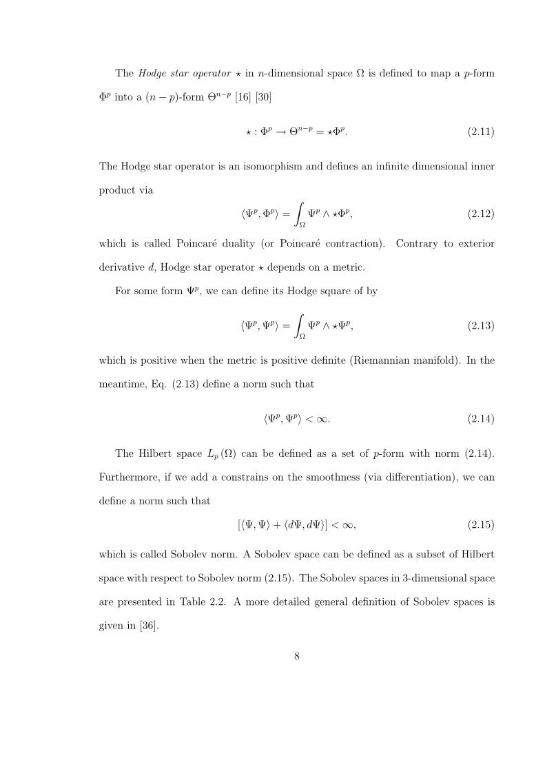
2.2 Sobolev spaces in 3-dimensional space. . . . . . . . . . . . . . . . . . 9

5.1 Galerkin duality vs. Electromagnetic duality. . . . . . . . . . . . . . . 54

5.2 Forms and elements of TE and TM. . . . . . . . . . . . . . . . . . . . 57

5.3 TE modes (angular frequencies of the five lowest nonzero modes) of acircular cavity. . . . . . . . . . . . . . . . . . . . . . . . . . . . . . . . 58

5.4 TM modes (angular frequencies of the five lowest nonzero modes) of acircular cavity. . . . . . . . . . . . . . . . . . . . . . . . . . . . . . . . 59

5.5 Numerical results for the number of modes in the TE and TM cases. . 59

5.6 TE modes (angular frequencies of the five lowest nonzero modes) of apolygonal cavity. . . . . . . . . . . . . . . . . . . . . . . . . . . . . . 60

5.7 TM modes (angular frequencies of the five lowest nonzero modes) of apolygonal cavity. . . . . . . . . . . . . . . . . . . . . . . . . . . . . . 61

5.8 Null spaces and range spaces of [XE] and [XH ]. . . . . . . . . . . . . 63

5.9 Eigenmodes of 3D spherical cavity . . . . . . . . . . . . . . . . . . . . 64

5.10 Eigenmodes of inhomogeneous cylindrical cavity . . . . . . . . . . . . 65

5.11 Number of modes from numerical results . . . . . . . . . . . . . . . . 67

xi

5.12 Null space and range space of [XE] and [XH ] . . . . . . . . . . . . . . 67

6.1 TE resonant frequencies of circular cavity via an algebraic-based spar-sification of the inverse mass matrix. . . . . . . . . . . . . . . . . . . 85

6.2 TM resonant frequencies of circular cavity via an algebraic-based spar-sification of the inverse mass matrix. . . . . . . . . . . . . . . . . . . 87

6.3 TE resonant frequencies of circular cavity via a topological-based spar-sification of the inverse mass matrix. . . . . . . . . . . . . . . . . . . 88

7.1 TE modes (angular frequencies ω of the five lowest nonzero modes) ofa circular cavity, computed by E-B mixed FEM. . . . . . . . . . . . . 93

7.2 TM modes (angular frequencies ω of the five lowest nonzero modes) ofa circular cavity, computed by E-B mixed FEM. . . . . . . . . . . . . 93

7.3 Eigenmodes of a spherical cavity, computed by E-B mixed FEM. . . 94

7.4 Numerical results of the center of the forbidden gap ω0 and the bandgapdω. . . . . . . . . . . . . . . . . . . . . . . . . . . . . . . . . . . . . . 97

8.1 Global (discrete) divergences of zero modes and nonzero modes. . . . 103

8.2 Comparison of a line vector (1-form) and a surface vector (2-form).The underlying differential forms are included in parenthesis, stressingthe different nature of the operators curl and div in each case. . . . . 104

8.3 Numerical results without and with gauging in primal space. . . . . . 107

8.4 Numerical results without and with gauging in dual space. . . . . . . 110

xii

LIST OF FIGURES

Figure Page

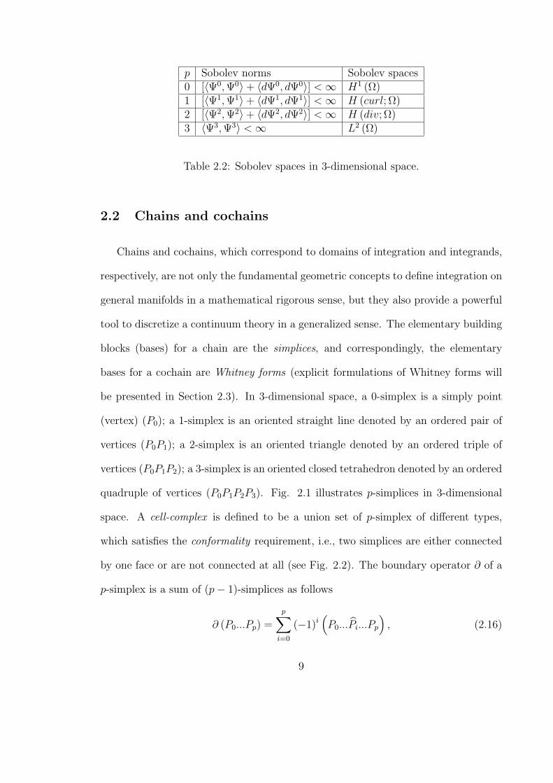
2.1 p-simplex in 3-dimensional space R3. . . . . . . . . . . . . . . . . . . 10

2.2 (a) Conformal; (b) non-conformal. . . . . . . . . . . . . . . . . . . . . 10

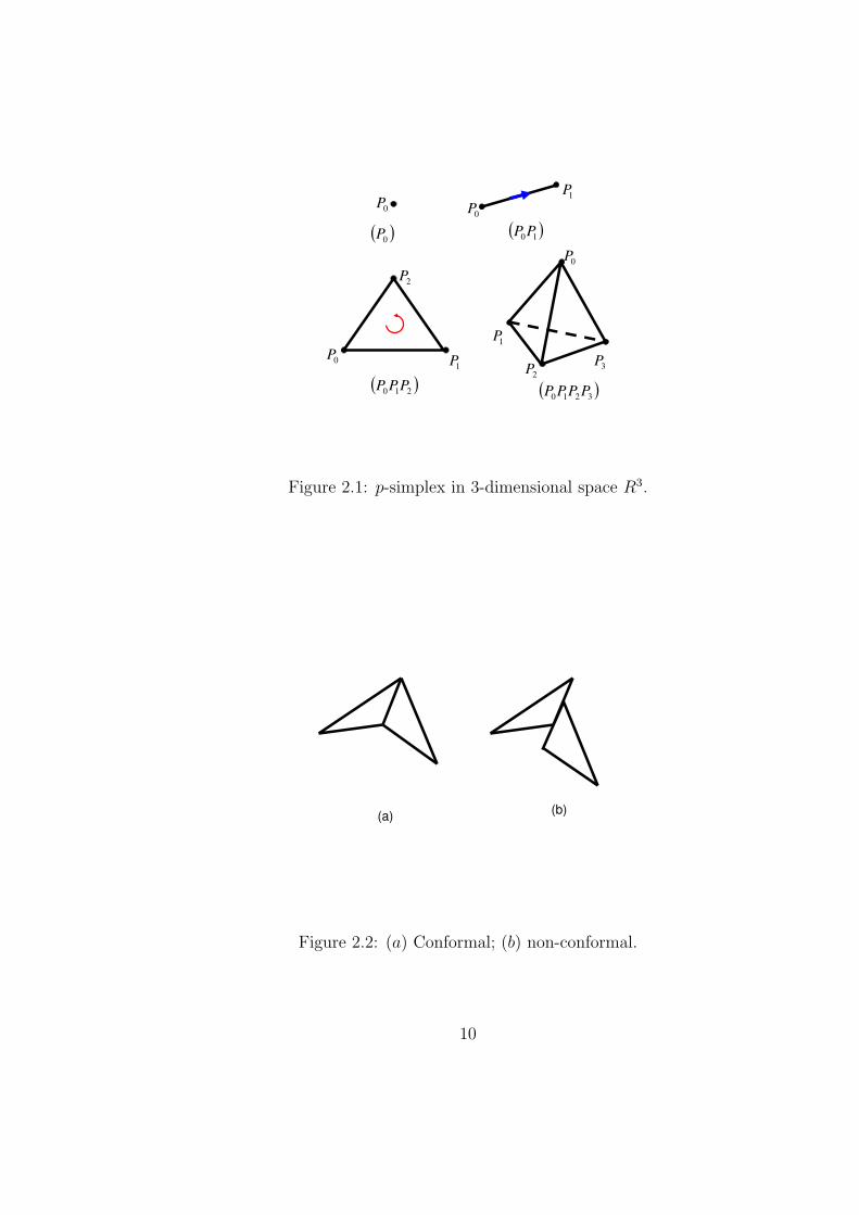
2.3 Boundary operator. . . . . . . . . . . . . . . . . . . . . . . . . . . . . 11

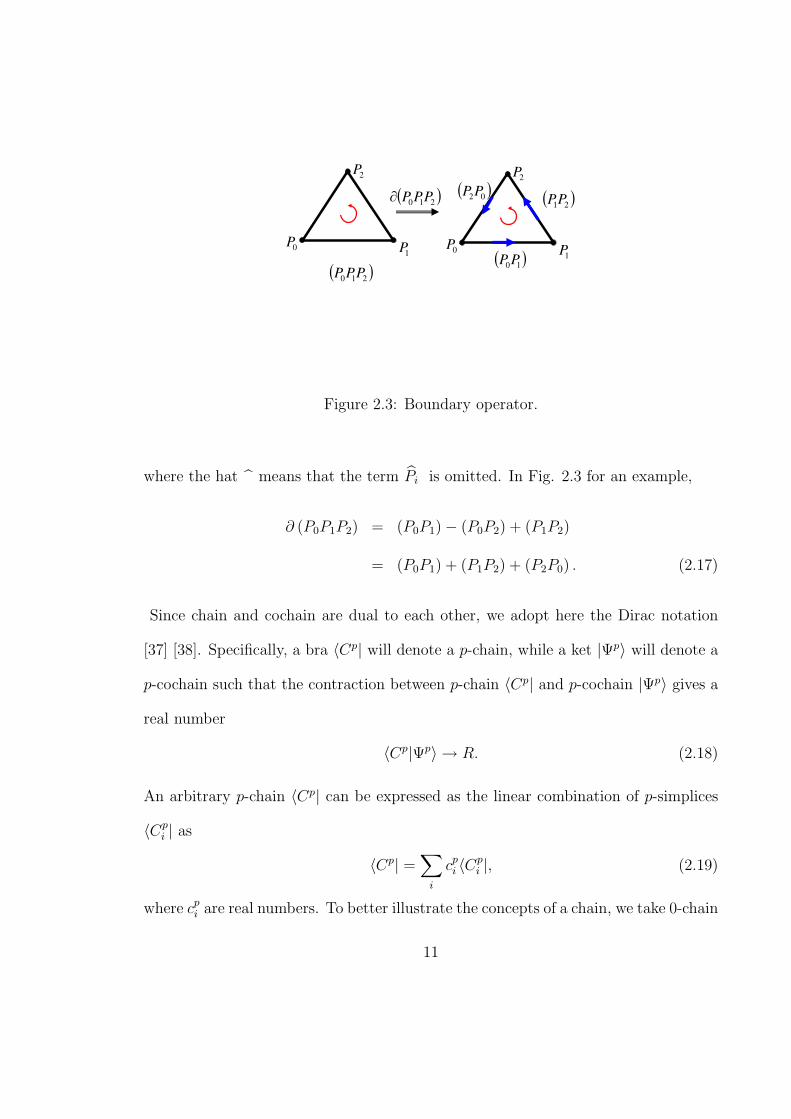
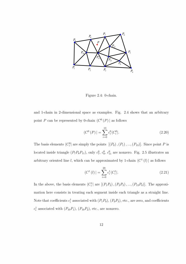
2.4 0-chain. . . . . . . . . . . . . . . . . . . . . . . . . . . . . . . . . . . 12

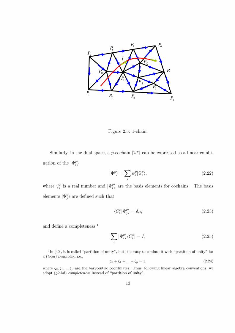
2.5 1-chain. . . . . . . . . . . . . . . . . . . . . . . . . . . . . . . . . . . 13

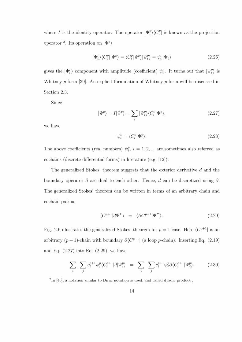
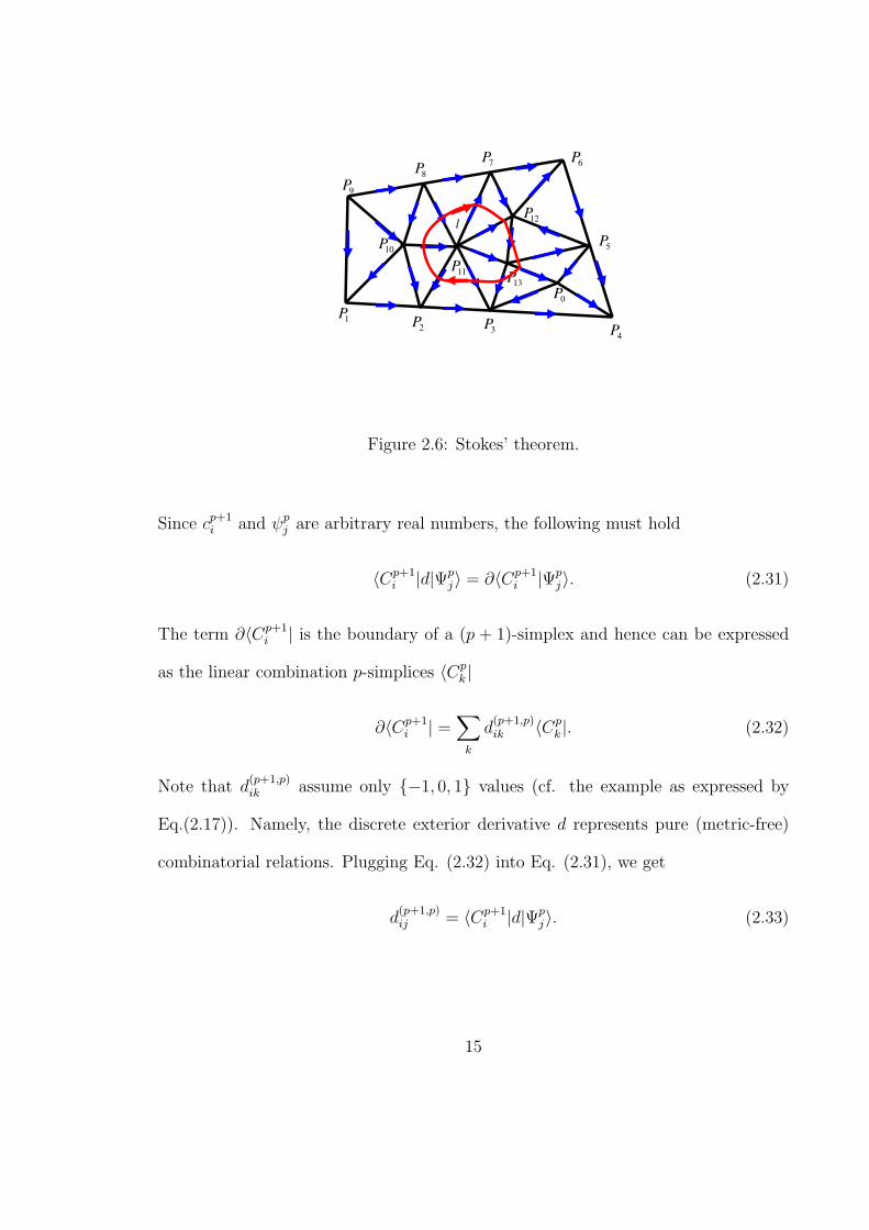
2.6 Stokes’ theorem. . . . . . . . . . . . . . . . . . . . . . . . . . . . . . . 15

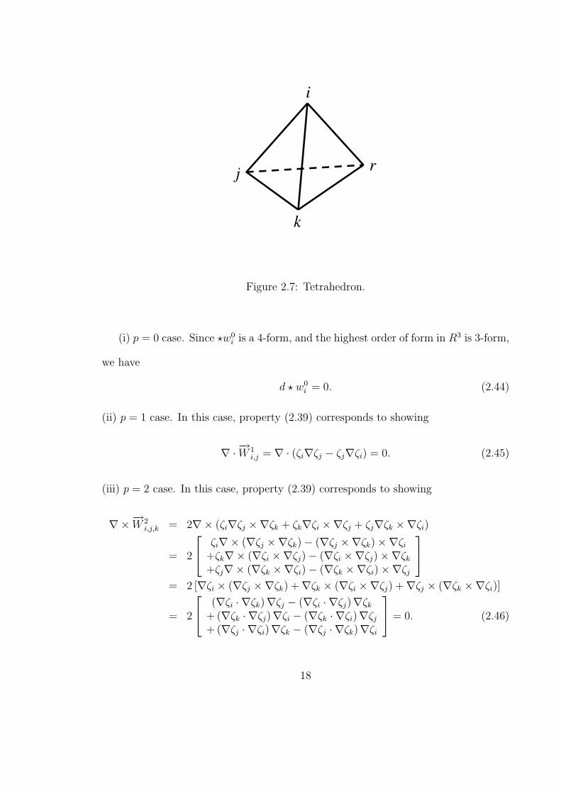
2.7 Tetrahedron. . . . . . . . . . . . . . . . . . . . . . . . . . . . . . . . . 18

3.1 The curved boundary ∂Ω is approximated by a set of linked edges ∂Ω. 24

3.2 Tiling the computation region with arbitrary polygons. . . . . . . . . 24

3.3 (a) conformal tiling (cell complex); (b) non-conformal tiling. . . . . . 25

3.4 Oriented polygons forming a cell complex. . . . . . . . . . . . . . . . 26

3.5 Solid lines represent the primal lattice. In 2D TE case, primal nodes(vertices) are paired with φ (e.g., node 1), primal edges with E (e.g.,edge 15) and primal faces with B (e.g., face 12345). Dashed lines rep-resent the dual lattice. Dual nodes are paired with H (e.g., node 4′),dual edges with (D, J) (e.g., edge 3′4′) and dual faces with Q (e.g.,face 1′2′3′4′5′). . . . . . . . . . . . . . . . . . . . . . . . . . . . . . . . 26

3.6 Oriented lattice. . . . . . . . . . . . . . . . . . . . . . . . . . . . . . . 28

xiii

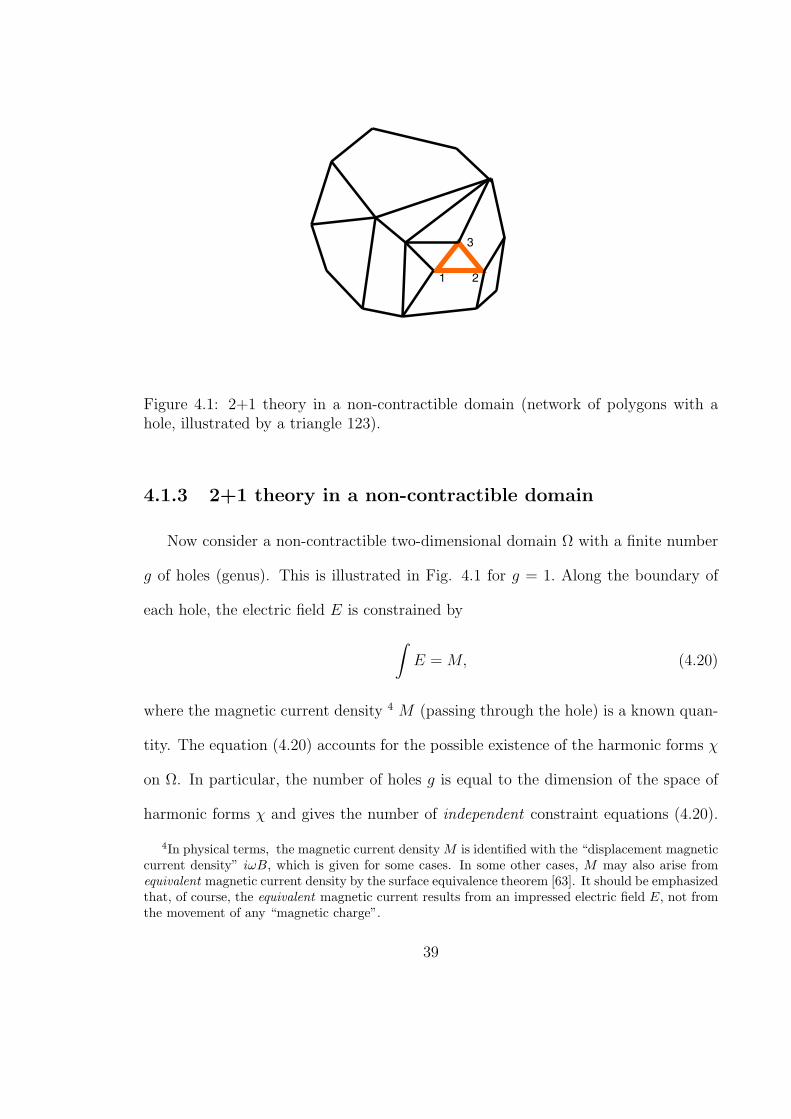
4.1 2+1 theory in a non-contractible domain (network of polygons with ahole, illustrated by a triangle 123). . . . . . . . . . . . . . . . . . . . 39

4.2 Yee lattice for the TE modes in a two-dimensional cavity with PECboundary. . . . . . . . . . . . . . . . . . . . . . . . . . . . . . . . . . 41

5.1 Triangular element. . . . . . . . . . . . . . . . . . . . . . . . . . . . . 50

5.2 Square element. . . . . . . . . . . . . . . . . . . . . . . . . . . . . . . 52

5.3 Mesh for a circular cavity, with 178 nodes (136 internal nodes), 447internal edges, and 312 cells. . . . . . . . . . . . . . . . . . . . . . . . 58

5.4 Mesh for a polygonal cavity. The coordinates of the vertices of thepolygon are (0, 0) , (1, 0) , (1.4, 0.4) , (1.3, 1.0) , (0.8, 1.2) , (0.3, 0.9). . . . 59

5.5 Mesh for a spherical cavity. . . . . . . . . . . . . . . . . . . . . . . . 64

5.6 Inhomogeneous 3D cylindrical cavity with dimensions a = 1, b = 0.1and d = 0.3. . . . . . . . . . . . . . . . . . . . . . . . . . . . . . . . 65

5.7 Mesh for a 3D inhomogeneous cylindrical cavity. . . . . . . . . . . . . 66

6.1 Plot of log10 (|−→χ i|) for an edge i near the center of a circular cavity,showing the strong localization property of −→χ i. . . . . . . . . . . . . 69

6.2 Plot of log10 (|−→χ i|) for edge i near the boundary of a circular cavity,showing the strong localization property of −→χ i. . . . . . . . . . . . . 69

6.3 Sparsity pattern of [?ε]−1a with r = 0.005. . . . . . . . . . . . . . . . . 72

6.4 Sparsity pattern of [?µ−1 ]−1a

with r = 0.005. . . . . . . . . . . . . . . . 72

6.5 Relative sparsification errors on the eigenvalues of [?ε]−1a with r = 0.005. 73

6.6 Relative sparsification errors on the eigenvalues of [?µ−1 ]−1a

with r =0.005. . . . . . . . . . . . . . . . . . . . . . . . . . . . . . . . . . . . 73

6.7 Relative truncation, sparsification, and total error on the FEM eigen-values. . . . . . . . . . . . . . . . . . . . . . . . . . . . . . . . . . . 75

xiv

6.8 Topological level-k neighbors (k = 0, 1, 2, ...) of edge (1, 2) in a 2D mesh.Level-0 neighbor includes only edge (1, 2). Level-1 neighbors includeedges (1, 2), (1, 4), (4, 2), (2, 3), and (1, 3). Level-2 neighbors includeedges (1, 2), (1, 4), (4, 2), (2, 3), (1, 3), (4, 7), (7, 1), (1, 6), (6, 3), (2, 8),(8, 4), (2, 5), and (5, 3). . . . . . . . . . . . . . . . . . . . . . . . . . . 76

6.9 Two FEM meshes for a circular cavity. Mesh (a) has 41 nodes and 64triangles. Mesh (b) has 178 nodes and 312 triangles. . . . . . . . . . . 77

6.10 Sparsity pattern of matrix [?ε]−1a in the coarse mesh case by using level-

k topological thresholding. (a) k = 0. (b) k = 1. (c) k = 2. (d) k = 3. 78

6.11 Relative sparsification error (star) in the coarse mesh case for eacheigenvalue, using level-k topological thresholding versus relative trun-cation error (diamond). (a) k = 0. (b) k = 1. (c) k = 2. and (d)k = 3. . . . . . . . . . . . . . . . . . . . . . . . . . . . . . . . . . . . 78

6.12 Sparsity pattern of [?ε]−1a in the fine mesh case by using level-k topo-

logical thresholding. (a) k = 0. (b) k = 1. (c) k = 2 and (d) k = 3. . 79

6.13 Relative sparsification error (stars) in the fine mesh case for each eigen-value, using level-k topological thresholding versus relative truncationerror (diamonds). (a) k = 0. (b) k = 1. (c) k = 2. and (d) k = 3. . . 80

6.14 Sparsity pattern of matrix [?ε]−1a for the mesh in Fig. 5.3 with r = 0.005. 83

6.15 Sparsity pattern of matrix [δcurl]a for the mesh in Fig. 5.3 with r = 0.005. 84

6.16 Eigenvalues of mass matrix [?ε]−1 (circle), and eigenvalues of [?ε]

−1a

(plus sign). The inset shows the relative errors (in percent) of eigen-values of [?ε]

−1a against the eigenvalues of [?ε]

−1. . . . . . . . . . . . . . 84

6.17 Density versus threshold r, and versus mesh sizes. Mesh 1 has 36 nodesand 50 cells. Mesh 2 has 178 nodes and 312 cells. Mesh 3 has 526 nodesand 968 cells. . . . . . . . . . . . . . . . . . . . . . . . . . . . . . . . 85

7.1 1D photonic crystal. . . . . . . . . . . . . . . . . . . . . . . . . . . . 96

7.2 Band structure of 1D photonic crystal. . . . . . . . . . . . . . . . . . 96

xv

8.1 2D cavity with multiple conductors. The size of the cavity is 1.0×0.95.C1 and C2 are both free conductors. . . . . . . . . . . . . . . . . . . . 101

8.2 Electrical field distributions for a cavity with multiple conductors. . 102

8.3 Tree-cotree splitting of a mesh for a rectangular cavity. The bold (redcolor) line edges represent tree edges. The remaining edges are cotreeedges (excluding the boundary edges). . . . . . . . . . . . . . . . . . 106

8.4 Sparsity patterns. (a) stiffness matrix after gauging; (b) mass matrixafter gauging. . . . . . . . . . . . . . . . . . . . . . . . . . . . . . . 107

8.5 Sparsity patterns. (a) sparsification of gauged stiffness matrix; (b)sparsification of gauged mass matrix. . . . . . . . . . . . . . . . . . . 108

8.6 Sparsification errors in gauged primal system. . . . . . . . . . . . . . 109

8.7 Sparsity patterns. (a) sparsification of gauged dual stiffness matrix;(b) sparsification of gauged dual mass matrix. . . . . . . . . . . . . . 110

8.8 Sparsification errors in gauged dual system. . . . . . . . . . . . . . . 111

8.9 Mesh for a circular cavity. The bold (red) line edge is the excitationedge. . . . . . . . . . . . . . . . . . . . . . . . . . . . . . . . . . . . . 112

8.10 Spectrum of electrical field in a circular cavity computed by time-domain solution of the discrete second order wave equation. (a) with-out gauging; (b) with gauging. . . . . . . . . . . . . . . . . . . . . . . 113

8.11 Evolution of the square root of discrete electrical field energy as afunction of time computed by the discrete second order wave equation.(a) without gauging; (b) with gauging. . . . . . . . . . . . . . . . . . 114

8.12 Tree-cotree splitting of a mesh for a circular cavity. The bold (red) lineedges are tree edges. The remaining edges are cotree edges (excludingthe boundary edges). . . . . . . . . . . . . . . . . . . . . . . . . . . . 115

8.13 Spectrum of electrical field in a circular cavity computed by first orderwave equation. (a) without gauging; (b) with gauging. . . . . . . . . 117

xvi

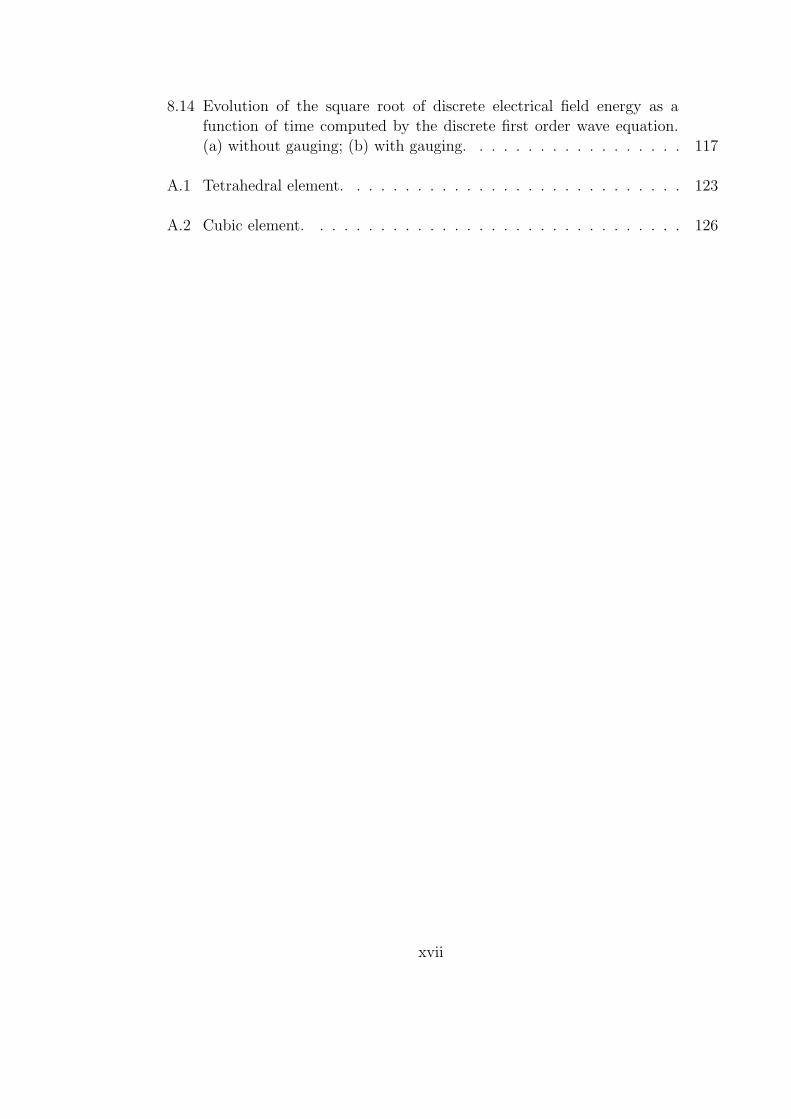
8.14 Evolution of the square root of discrete electrical field energy as afunction of time computed by the discrete first order wave equation.(a) without gauging; (b) with gauging. . . . . . . . . . . . . . . . . . 117

A.1 Tetrahedral element. . . . . . . . . . . . . . . . . . . . . . . . . . . . 123

A.2 Cubic element. . . . . . . . . . . . . . . . . . . . . . . . . . . . . . . 126

xvii

CHAPTER 1

INTRODUCTION

1.1 Background and motivation

Maxwell equations, as a continuum field theory, is a dynamical system having an

infinite number of degrees of freedom (DoF s). However, a computer is a machine

which can only process a finite number of DoF s. Thus any computational method

needs to discretize Maxwell equations by reducing it to a system of finite DoF s.

Currently, there are three main approaches to discretize Maxwell equations directly:

finite differences [1] [2], finite elements [3] [4] [5] [6] [7], and finite volumes [2]. Naive

implementations of these finite methods to discretize Maxwell equations on irregular

lattices are known to cause problems, such as spurious modes [8] [9], late-time un-

conditional instabilities [10], and low-frequency instabilities [11] that can destroy the

solutions. This is often a consequence of the failure to capture some essential physics

of the continuum theory. These drawbacks of finite methods motivate the construc-

tion of discrete Maxwell equations on a general lattice that inherit and mimic the

essential physical structure of the continuum theory.

1

We shall study discrete Maxwell equations using some basic tools of algebraic

topology and a discrete analog of differential forms [7] [12] [13]. We denote this ap-

proach a compatible discretization. This approach is somewhat close to the method-

ology of mimetic discretizations [14] (a generalized finite difference for irregular grids

based on approximating the vector calculus operators grad, curl, and div). Compared

to the mimetic discretizations, however, compatible discretization is a more general

framework. This is because both finite differences (including mimetic discretiza-

tion), finite elements, finite volumes, and even the finite integration technique [15]

can be studied in this framework. All these different discretization methods (im-

plicitly) adopt similar procedures to construct discrete exterior derivatives (incidence

matrices) which unify the various operators of vector calculus. The main differences

between the various discretization methods reside on the approach used to construct

discrete Hodge operators (which include all metric information).

1.2 Organization of this dissertation

This dissertation is organized as follows.

In Chapter 2, we present a brief review of differential forms and some fundamental

concepts of algebraic topology. The key bridge connecting a continuum differential

form and its discrete counterpart is provided by the so-called Whitney forms. Hence,

we also discuss some essential properties of Whitney forms.

In Chapter 3, we first formulate Maxwell equations and constitutive relations using

differential forms. Next, we illustrate how to obtain a general compatible discretiza-

tion for Maxwell equations in an arbitrary network of polygons for 2D (polyhedra

2

for 3D). We then discretize the constitutive equations (discrete Hodge operators) on

tetrahedra and cubes.

In Chapter 4, based on the general compatible discretizations for Maxwell equa-

tions on irregular grids introduced in Chapter 3, we show that Euler’s formula matches

the algebraic properties of the discrete Hodge decomposition in an exact way. Fur-

thermore, we show that the number of dynamic DoFs for the electric field equals the

number of dynamic DoFs for the magnetic field, which reflects one of the essential

properties of discrete Maxwell equations (a constrained Hamiltonian system).

In Chapter 5, we unveil a duality called Galerkin duality, a mathematical transfor-

mation between electric field intensity E and magnetic field intensity H. For concrete-

ness, Galerkin Hodges are realized as discrete Hodge operators. We construct two

dual system matrices, [XE] (primal formulation) and [XH ] (dual formulation), respec-

tively, that discretize Maxwell equations in terms of the electric field and magnetic

field, respectively. We show that the primal formulation recovers the conventional

(edge-element) finite element method (FEM) and suggests a geometric foundation for

it. On the other hand, the dual formulation suggests a new (dual) type of FEM. Al-

though both formulations give identical physical solutions, the dimensions of the null

spaces are different. Algebraic relationships among the degrees of freedom of primal

and dual FEM formulations are explained using a discrete version of the Hodge de-

composition and Euler’s formula for a network of polygons for 2D case and polyhedra

for 3D case.

In Chapter 6, we further investigate discrete Hodge operators properties. We find

that although Hodge matrices (e.g., Galerkin’s Hodges) are sparse, their inverses are

in general not sparse on irregular grids . However, we find that the inverse Hodge

3

matrices are quasi-sparse (strong localization properties). Therefore, we introduce

two sparsification approaches, which are denoted algebraic thresholding and topo-

logical thresholding, to approximate the inverse Hodge matrices by sparse matrices.

Based on these sparsifications, an explicit and sparse FETD scheme is proposed. The

topological thresholding technique also provides a very general and systematic way

to derive stable local finite-difference stencils in irregular meshes.

In Chapter 7, we construct a mixed FEM scheme for Maxwell equations, which

is based on using the electric field intensity−→E and magnetic field flux

−→B (instead

of magnetic field intensity−→H ) as state variables simultaneously. In this scheme,

edge elements are used as the interpolants for the electric field intensity−→E and face

elements as the interpolants for the magnetic flux−→B . In contrast to E-H mixed

FEM, this new mixed FEM results in sparse matrices.

In Chapter 8, motivated in solving low-frequency instability problems in frequency

domain FEM and in eliminating spurious solutions with linear time growth in time

domain FEM, we analyze singularities arising from the null space of the (discrete)

curl operator. We define global discrete divergence and global gauging. Based on

global gauging, we propose approaches to treat (at least from theoretical point of

view) low-frequency instabilities and spurious linear time growth in FEM.

In Chapter 9, we summarize the main contributions of this dissertation.

4

CHAPTER 2

MATHEMATICAL PRELIMINARIES

In this Chapter, we first give a brief review of differential forms [16] [17] [18] [19]

[20]. One can also refer to [21] [22] [23] [24] [25] [26] for differential forms applied to

electromagnetics. We then introduce some fundamental tools of algebraic topology,

in particular, chains and cochains [27] [28] [29]. Cochains can be viewed as discrete

differential forms. For a more detailed discussion on discrete differential forms, one

can refer to [12] [13] [30] [31] [32] [33] [34]. Since the key bridge connecting a contin-

uum differential form and its discrete counterpart is Whitney forms [27] [35], we also

discuss some of essential properties of Whitney forms.

2.1 Differential forms

In electromagnetics, as well as other branches of physics, one often finds the

need to integrate a physical quantity over a line, a surface, or a volume. Differential

forms provide a unified approach to integrate a physical quantity over a p-dimensional

manifold in n-dimensional space. For example, the line integral for electrical field

intensity−→E ∫

l

−→E · dl =

∫

l

Exdx + Eydy + Ezdz, (2.1)

5

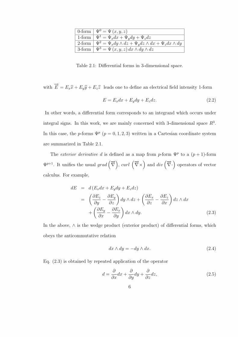
0-form Ψ0 = Ψ (x, y, z)1-form Ψ1 = Ψxdx + Ψydy + Ψzdz2-form Ψ2 = Ψxdy ∧ dz + Ψydz ∧ dx + Ψzdx ∧ dy3-form Ψ3 = Ψ (x, y, z) dx ∧ dy ∧ dz

Table 2.1: Differential forms in 3-dimensional space.

with−→E = Exx + Eyy + Ez z leads one to define an electrical field intensity 1-form

E = Exdx + Eydy + Ezdz. (2.2)

In other words, a differential form corresponds to an integrand which occurs under

integral signs. In this work, we are mainly concerned with 3-dimensional space R3.

In this case, the p-forms Ψp (p = 0, 1, 2, 3) written in a Cartesian coordinate system

are summarized in Table 2.1.

The exterior derivative d is defined as a map from p-form Ψp to a (p + 1)-form

Ψp+1. It unifies the usual grad(−→∇

), curl

(−→∇×)

and div(−→∇·

)operators of vector

calculus. For example,

dE = d (Exdx + Eydy + Ezdz)

=

(∂Ez

∂y− ∂Ey

∂z

)dy ∧ dz +

(∂Ex

∂z− ∂Ez

∂x

)dz ∧ dx

+

(∂Ey

∂x− ∂Ex

∂y

)dx ∧ dy. (2.3)

In the above, ∧ is the wedge product (exterior product) of differential forms, which

obeys the anticommutative relation

dx ∧ dy = −dy ∧ dx. (2.4)

Eq. (2.3) is obtained by repeated application of the operator

d =∂

∂xdx +

∂

∂ydy +

∂

∂zdz, (2.5)

6

over each scalar component, e.g., Ex, Ey, Ez.

Note that in Eq. (2.3), terms such as ∂Ex

∂xdx ∧ dx, ∂Ey

∂ydy ∧ dy, ∂Ez

∂zdz ∧ dz are

excluded due to the anticommutative relation (2.4). It can be shown that

ddE = 0. (2.6)

This corresponds to vector calculus identity

−→∇ · −→∇ ×−→E = 0. (2.7)

Property (2.6) can be generalized to any p-form Ψp:

ddΨp = 0, (2.8)

which is known as Poincare lemma [16]. It should be noted that exterior derivative

d is metric-free and independent of a coordinate system. Its rigorous mathematical

definition is established by the generalized Stokes’ theorem [27].

An integral is defined as a contraction between a p-form Ψp and a p-dimensional

manifold Cp, which can be denoted as

〈Cp, Ψp〉 =

∫

Cp

Ψp, (2.9)

which gives a real number as result. The definition (2.9) suggests that p-form Ψp

can be considered as belonging to the dual (vector) space of Cp. Let ∂Cp+1 be

the boundary (to be defined explicitly in the next Section) of a (p + 1)-dimensional

manifold Cp+1. The generalized Stokes’ theorem can be written as

⟨Cp+1, dΨp

⟩=

⟨∂Cp+1, Ψp

⟩. (2.10)

In 3-dimensional space, it unifies the usual vector calculus versions of gradient theo-

rem, divergence (or Gauss’s theorem) and Stokes’ theorem.

7

The Hodge star operator ? in n-dimensional space Ω is defined to map a p-form

Φp into a (n− p)-form Θn−p [16] [30]

? : Φp → Θn−p = ?Φp. (2.11)

The Hodge star operator is an isomorphism and defines an infinite dimensional inner

product via

〈Ψp, Φp〉 =

∫

Ω

Ψp ∧ ?Φp, (2.12)

which is called Poincare duality (or Poincare contraction). Contrary to exterior

derivative d, Hodge star operator ? depends on a metric.

For some form Ψp, we can define its Hodge square of by

〈Ψp, Ψp〉 =

∫

Ω

Ψp ∧ ?Ψp, (2.13)

which is positive when the metric is positive definite (Riemannian manifold). In the

meantime, Eq. (2.13) define a norm such that

〈Ψp, Ψp〉 < ∞. (2.14)

The Hilbert space Lp (Ω) can be defined as a set of p-form with norm (2.14).

Furthermore, if we add a constrains on the smoothness (via differentiation), we can

define a norm such that

[〈Ψ, Ψ〉+ 〈dΨ, dΨ〉] < ∞, (2.15)

which is called Sobolev norm. A Sobolev space can be defined as a subset of Hilbert

space with respect to Sobolev norm (2.15). The Sobolev spaces in 3-dimensional space

are presented in Table 2.2. A more detailed general definition of Sobolev spaces is

given in [36].

8

p Sobolev norms Sobolev spaces0 [〈Ψ0, Ψ0〉+ 〈dΨ0, dΨ0〉] < ∞ H1 (Ω)1 [〈Ψ1, Ψ1〉+ 〈dΨ1, dΨ1〉] < ∞ H (curl; Ω)2 [〈Ψ2, Ψ2〉+ 〈dΨ2, dΨ2〉] < ∞ H (div; Ω)3 〈Ψ3, Ψ3〉 < ∞ L2 (Ω)

Table 2.2: Sobolev spaces in 3-dimensional space.

2.2 Chains and cochains

Chains and cochains, which correspond to domains of integration and integrands,

respectively, are not only the fundamental geometric concepts to define integration on

general manifolds in a mathematical rigorous sense, but they also provide a powerful

tool to discretize a continuum theory in a generalized sense. The elementary building

blocks (bases) for a chain are the simplices, and correspondingly, the elementary

bases for a cochain are Whitney forms (explicit formulations of Whitney forms will

be presented in Section 2.3). In 3-dimensional space, a 0-simplex is a simply point

(vertex) (P0); a 1-simplex is an oriented straight line denoted by an ordered pair of

vertices (P0P1); a 2-simplex is an oriented triangle denoted by an ordered triple of

vertices (P0P1P2); a 3-simplex is an oriented closed tetrahedron denoted by an ordered

quadruple of vertices (P0P1P2P3). Fig. 2.1 illustrates p-simplices in 3-dimensional

space. A cell-complex is defined to be a union set of p-simplex of different types,

which satisfies the conformality requirement, i.e., two simplices are either connected

by one face or are not connected at all (see Fig. 2.2). The boundary operator ∂ of a

p-simplex is a sum of (p− 1)-simplices as follows

∂ (P0...Pp) =

p∑i=0

(−1)i(P0...Pi...Pp

), (2.16)

9

0P 10

PP

210PPP

1P

0P0

P

0P

1P

2P

0P

2P 3

P

1P

3210PPPP

Figure 2.1: p-simplex in 3-dimensional space R3.

(a)(b)

Figure 2.2: (a) Conformal; (b) non-conformal.

10

10PP

0P

1P

2P

210PPP

0P

1P

2P

02PP

21PP210

PPP

Figure 2.3: Boundary operator.

where the hat means that the term Pi is omitted. In Fig. 2.3 for an example,

∂ (P0P1P2) = (P0P1)− (P0P2) + (P1P2)

= (P0P1) + (P1P2) + (P2P0) . (2.17)

Since chain and cochain are dual to each other, we adopt here the Dirac notation

[37] [38]. Specifically, a bra 〈Cp| will denote a p-chain, while a ket |Ψp〉 will denote a

p-cochain such that the contraction between p-chain 〈Cp| and p-cochain |Ψp〉 gives a

real number

〈Cp|Ψp〉 → R. (2.18)

An arbitrary p-chain 〈Cp| can be expressed as the linear combination of p-simplices

〈Cpi | as

〈Cp| =∑

i

cpi 〈Cp

i |, (2.19)

where cpi are real numbers. To better illustrate the concepts of a chain, we take 0-chain

11

1P

0P

13P

12P

11P

10P

9P

8P

7P

6P

5P

4P3

P2P

P

Figure 2.4: 0-chain.

and 1-chain in 2-dimensional space as examples. Fig. 2.4 shows that an arbitrary

point P can be represented by 0-chain 〈C0 (P ) | as follows

〈C0 (P ) | =13∑i=0

c0i 〈C0

i |. (2.20)

The basis elements 〈C0i | are simply the points [(P0) , (P1) , ..., (P13)]. Since point P is

located inside triangle (P7P8P11), only c07, c0

8, c011 are nonzero. Fig. 2.5 illustrates an

arbitrary oriented line l, which can be approximated by 1-chain 〈C1 (l) | as follows

〈C1 (l) | =29∑i=0

c1i 〈C1

i |. (2.21)

In the above, the basis elements 〈C1i | are [(P1P2) , (P2P3) , ..., (P13P0)]. The approxi-

mation here consists in treating each segment inside each triangle as a straight line.

Note that coefficients c1i associated with (P1P9), (P0P3), etc., are zero, and coefficients

c1i associated with (P10P1), (P10P2), etc., are nonzero.

12

1P

0P

13P

12P

11P

10P

9P

8P

7P

6P

5P

4P3

P2P

l

Figure 2.5: 1-chain.

Similarly, in the dual space, a p-cochain |Ψp〉 can be expressed as a linear combi-

nation of the |Ψpi 〉

|Ψp〉 =∑

i

ψpi |Ψp

i 〉, (2.22)

where ψpi is a real number and |Ψp

i 〉 are the basis elements for cochains. The basis

elements |Ψpj〉 are defined such that

〈Cpi |Ψp

j〉 = δij, (2.23)

and define a completeness 1

∑i

|Ψpi 〉〈Cp

i | = I, (2.25)

1In [40], it is called “partition of unity”, but it is easy to confuse it with “partition of unity” fora (local) p-simplex, i.e.,

ζ0 + ζ1 + ... + ζp = 1, (2.24)

where ζ0, ζ1, ..., ζp are the barycentric coordinates. Thus, following linear algebra conventions, weadopt (global) completeness instead of “partition of unity”.

13

where I is the identity operator. The operator |Ψpi 〉〈Cp

i | is known as the projection

operator 2. Its operation on |Ψp〉

|Ψpi 〉〈Cp

i ||Ψp〉 = 〈Cpi |Ψp〉|Ψp

i 〉 = ψpi |Ψp

i 〉 (2.26)

gives the |Ψpi 〉 component with amplitude (coefficient) ψp

i . It turns out that |Ψpi 〉 is

Whitney p-form [39]. An explicit formulation of Whitney p-form will be discussed in

Section 2.3.

Since

|Ψp〉 = I|Ψp〉 =∑

i

|Ψpi 〉〈Cp

i |Ψp〉, (2.27)

we have

ψpi = 〈Cp

i |Ψp〉. (2.28)

The above coefficients (real numbers) ψpi , i = 1, 2, ... are sometimes also referred as

cochains (discrete differential forms) in literature (e.g. [12]).

The generalized Stokes’ theorem suggests that the exterior derivative d and the

boundary operator ∂ are dual to each other. Hence, d can be discretized using ∂.

The generalized Stokes’ theorem can be written in terms of an arbitrary chain and

cochain pair as

〈Cp+1|dΨP 〉 =⟨∂Cp+1|ΨP

⟩. (2.29)

Fig. 2.6 illustrates the generalized Stokes’ theorem for p = 1 case. Here 〈Cp+1| is an

arbitrary (p + 1)-chain with boundary ∂〈Cp+1| (a loop p-chain). Inserting Eq. (2.19)

and Eq. (2.27) into Eq. (2.29), we have

∑i

∑j

cp+1i ψp

j 〈Cp+1i |d|Ψp

j〉 =∑

i

∑j

cp+1i ψp

j ∂〈Cp+1i |Ψp

j〉. (2.30)

2In [40], a notation similar to Dirac notation is used, and called dyadic product .

14

1P

0P

13P

12P

11P

10P

9P

8P

7P

6P

5P

4P3

P2P

l

Figure 2.6: Stokes’ theorem.

Since cp+1i and ψp

j are arbitrary real numbers, the following must hold

〈Cp+1i |d|Ψp

j〉 = ∂〈Cp+1i |Ψp

j〉. (2.31)

The term ∂〈Cp+1i | is the boundary of a (p + 1)-simplex and hence can be expressed

as the linear combination p-simplices 〈Cpk |

∂〈Cp+1i | =

∑

k

d(p+1,p)ik 〈Cp

k |. (2.32)

Note that d(p+1,p)ik assume only −1, 0, 1 values (cf. the example as expressed by

Eq.(2.17)). Namely, the discrete exterior derivative d represents pure (metric-free)

combinatorial relations. Plugging Eq. (2.32) into Eq. (2.31), we get

d(p+1,p)ij = 〈Cp+1

i |d|Ψpj〉. (2.33)

15

2.3 Whitney forms

Consider an oriented n-simplex described by barycentric coordinates (ζ0, ..., ζn) .

The Whitney p-form |Ψpj〉 can be written in terms of barycentric coordinates as [27]

|Ψpj〉 = wp

ζ0,...,ζp= p!

p∑i=0

(−1)i ζidζ0 ∧ ... ∧ dζi ∧ ... ∧ dζp, (2.34)

where the hat means that the term dζi is omitted. In the rest of this section, we

shall discuss some of the fundamental properties of Whitney forms.

2.3.1 Recursive (generating) relation

Let wp−1

ζ0,...,bζi,...,ζpdenote a Whitney (p− 1)-form such that the index ζi is omitted.

Below, we use the example of a face (ζ0, ζ1, ζ2) on a tetrahedron (ζ0, ζ1, ζ2, ζ3) to illus-

trate the above definition. According to (2.34), the Whitney form for face (ζ0, ζ1, ζ2)

is written as

w2ζ0,ζ1,ζ2

= 2!2∑

i=0

(−1)i ζidζ0 ∧ ... ∧ dζi ∧ ... ∧ dζ2

= 2ζ0dζ1 ∧ dζ2 − 2ζ1dζ0 ∧ dζ2 + 2ζ2dζ0 ∧ dζ1. (2.35)

There are 3 edges on the face (ζ0, ζ1, ζ2). The 3 edges can be denoted as (ζ0, ζ1) ,

(ζ0, ζ2) , (ζ1, ζ2), which can also be denoted as(ζ0, ζ1, ζ2

),

(ζ0, ζ1, ζ2

),(ζ0, ζ1, ζ2

).

The Whitney form for edge(ζ0, ζ1, ζ2

)can be denoted as w1

ζ0,ζ1, bζ2 .

Applying exterior derivative operator d to wp−1

ζ0,...,bζi,...,ζpgives

dwp−1

ζ0,...,bζi,...,ζp= p!dζ0 ∧ ... ∧ dζi ∧ ... ∧ dζp. (2.36)

Plugging Eq.(2.36) into (2.34), we obtain a recursive relation between Whitney p-form

and Whitney (p− 1)-form as

wpζ0,...,ζr

=

p∑i=0

(−1)i ζidwp−1

ζ0,...,bζi,...,ζr. (2.37)

16

For 3D case, this recursive relation (2.37) coincides with the generation relation ex-

pressed in terms of incidence matrices [41]. This recursive relation suggests that one

can generate p-forms (p = 1, 2, ..., n) from 0-forms. We use Whitney edge form (1-

form) and face form (2-form) on a tetrahedron as an example to illustrate the above

recursive relation. We can check (2.37) by computing face form w2ζ0,ζ1,ζ2

w2ζ0,ζ1,ζ2

=2∑

i=0

(−1)i ζidw1ζ0,...,bζi,...,ζ2

= ζ0dw1bζ0,ζ1,ζ2

− ζ1dw1ζ0, bζ1,ζ2

+ ζ2dw1ζ0,ζ1, bζ2

= ζ0d (ζ1dζ2 − ζ2dζ1)− ζ1d (ζ0dζ2 − ζ2dζ0) + ζ2d (ζ0dζ1 − ζ1dζ0)

= 2ζ0dζ1dζ2 − 2ζ1dζ0dζ2 + 2ζ2dζ0dζ1 (2.38)

2.3.2 Local gauging property

Whitney forms have the property

d ? wpζ0,...,ζp

= 0. (2.39)

that we denote local gauging property. We next consider Eq. (2.39) in 3-dimensional

space. For a tetrahedron (3-simplex) (Fig. 2.7), we use ordered indexing of nodes

to denote the vertices (e.g., i), oriented edges (e.g., i, j), oriented faces (e.g., i, j, k)

and oriented cells (e.g., i, j, k, r). Thus Whitney forms are indexed as w0i , w1

i,j, w2i,j,k,

w3i,j,k,r. The vector calculus proxies of Whitney forms can be similarly denoted as

W 0i ,−→W 1

i,j,−→W 2

i,j,k,W3i,j,k,r, and are found by replacing d with ∇, i.e.,

W 0i = ζi, (2.40)

−→W 1

i,j = ζi∇ζj − ζj∇ζi, (2.41)

−→W 2

i,j,k = 2 (ζi∇ζj ×∇ζk + ζj∇ζk ×∇ζi + ζk∇ζi ×∇ζj) , (2.42)

W 3i,j,k,r = 6

(ζi∇ζj ×∇ζk ×∇ζr − ζr∇ζi ×∇ζj ×∇ζk

+ζk∇ζr ×∇ζi ×∇ζj − ζj∇ζk ×∇ζr ×∇ζi

). (2.43)

17

k

i

jr

Figure 2.7: Tetrahedron.

(i) p = 0 case. Since ?w0i is a 4-form, and the highest order of form in R3 is 3-form,

we have

d ? w0i = 0. (2.44)

(ii) p = 1 case. In this case, property (2.39) corresponds to showing

∇ · −→W 1i,j = ∇ · (ζi∇ζj − ζj∇ζi) = 0. (2.45)

(iii) p = 2 case. In this case, property (2.39) corresponds to showing

∇×−→W 2i,j,k = 2∇× (ζi∇ζj ×∇ζk + ζk∇ζi ×∇ζj + ζj∇ζk ×∇ζi)

= 2

ζi∇× (∇ζj ×∇ζk)− (∇ζj ×∇ζk)×∇ζi

+ζk∇× (∇ζi ×∇ζj)− (∇ζi ×∇ζj)×∇ζk

+ζj∇× (∇ζk ×∇ζi)− (∇ζk ×∇ζi)×∇ζj

= 2 [∇ζi × (∇ζj ×∇ζk) +∇ζk × (∇ζi ×∇ζj) +∇ζj × (∇ζk ×∇ζi)]

= 2

(∇ζi · ∇ζk)∇ζj − (∇ζi · ∇ζj)∇ζk

+ (∇ζk · ∇ζj)∇ζi − (∇ζk · ∇ζi)∇ζj

+ (∇ζj · ∇ζi)∇ζk − (∇ζj · ∇ζk)∇ζi

= 0. (2.46)

18

(iv) p = 3 case. Since the 3-form w3i,j,k,r is a constant in cell (tetrahedron),

d ? w3i,j,k,r = 0. (2.47)

follows trivially.

2.3.3 De Rham diagram (exact sequence property)

The Sobolev spaces (see Table 2.2) observe the following de Rham diagram [48]

[53] [6] [5]

H1 (Ω)d7→ H (curl, Ω)

d7→ H (div, Ω)d7→ L2 (Ω) . (2.48)

Moreover, by assuming that domain Ω is contractible, the range of each operator

is the null space of next operator in the sequence. Let W 0, W 1, W 2, and W 3 the

Whitney spaces spanned by W 0i ,−→W 1

i,j,−→W 2

i,j,k, and W 3i,j,k,r, respectively. The Whitney

spaces observe the discrete de Rham diagram

W 0 ∇7→ W 1 ∇×7→ W 2 ∇·7→ W 3. (2.49)

2.3.4 Whitney elements in local coordinates

Let

−→r = xx + yy + zz (2.50)

denote a point in space. In terms of x, y, z, Whitney elements, denoted as W 0(x, y, z),

−→W 1 (x, y, z),

−→W 2 (x, y, z), W 3 (x, y, z), can be written as [5]

W 0(x, y, z) = a0 +−→b 0 · −→r , (2.51)

−→W 1 (x, y, z) = −→a 1 +

−→b 1 ×−→r , (2.52)

−→W 2 (x, y, z) = −→a 2 + b2−→r , (2.53)

W 3 (x, y, z) = a3, (2.54)

19

where ai and bi are constant real numbers, and −→a i and−→b i are constant real vectors.

In a finite element (FEM) setting, the above Whitney elements representations are

also called shape functions. The applications of Whitney elements for FEM solutions

of electromagnetics can be found in [3] [4] [5] [6] [7]. Whitney elements−→W 1 (x, y, z)

and−→W 2 (x, y, z) were rediscovered in mixed FEM in [42] [43] [44] [45]. Whitney

elements−→W 1 (x, y, z) twisted by π

2in 2D also appeared in [46] in connection with

the numerical solution of integral equations via the method of moments. Whitney

element−→W 1 (x, y, z) was first applied to electromagnetic problems in [47]. The con-

nection between Whitney elements W 0(x, y, z),−→W 1 (x, y, z),

−→W 2 (x, y, z), W 3 (x, y, z)

as expressed above and W 0i ,−→W 1

i,j,−→W 2

i,j,k,W3i,j,k,r was discussed in [7].

20

CHAPTER 3

COMPATIBLE DISCRETIZATIONS FOR MAXWELLEQUATIONS

By applying some tools of algebraic topology and discrete differential forms, clas-

sical electromagnetics can be constructed from first principles on an arbitrary lattice.

The fundamental concepts of algebraic topology used here are chains and cochains,

which represent discrete domains of integration and integrands (discrete differential

forms), respectively. An arbitrary domain of integration can be approximated by a

linear combination of p-simplices; It follows that the corresponding (dual) differential

form can be approximated by a linear combination of fundamental discrete p-forms

as

Ψp =∑

i

ψpi w

pi , (3.1)

where ψpi are real numbers and wp

i are the bases (elemental discrete p-forms) for the

p-cochain. As discussed in Chapter 2, these elemental discrete p-forms wpi are the

Whitney forms [39]. The coefficients ψpi are the results of contraction between the

p-simplex Cpi and cochain Ψp

ψpi = 〈Cp

i , Ψp〉 . (3.2)

The ψpi , i = 1, 2, ... are sometimes also called cochains (discrete differential forms),

e.g. [12]. The two fundamental operators the exterior derivative d and the Hodge star

21

operator ? can be discretized by employing two duality relations. By applying the

duality between chain and cochain and the discrete Stokes’ theorem, one can obtain

discrete exterior derivative d directly from the boundary operator ∂. On the other

hand, the discrete Poincare duality, which is a duality between discrete differential

forms defined on primal lattice and dual lattice, provides a mechanism to discretize

the Hodge operator. The above constructions have been well established for simplicial

complex in mathematical literature (cf. Chapter 2 for detail and the references). In

computational electromagnetics as well as other areas of computational physics, the

consideration of nonsimplicial complexes such as hexahedral (in both FDTD [2] [1] and

FEM [3]), pyramidal (in FEM) [54], even mixed polygonal [55] are often used. Thus, in

this Chapter, we will consider the compatible discretization of Maxwell equations in a

general cell-complex (e.g., a network of mixed polygons for 2D or mixed polyhedra for

3D). However, considerations about the metric part of electromagnetics (constitutive

equations) will be limited to simplicial and cubic complexes because discrete Hodge

operators are well defined on these cases.

3.1 Maxwell equations in differential forms language

Maxwell equations (in the Fourier domain) are written in terms of differential

forms as [21] [7] [12]

dE = iωB, dB = 0, dH = −iωD + J, dD = Q, (3.3)

where E and H are electric and magnetic field intensity 1-forms, D and B are electric

and magnetic flux 2-forms, and J is the electric current density 2-form, and Q is the

electric charge density 3-form, and d is the (metric-free) exterior derivative operator.

From the identity d2 = 0, the electric current density J and the charge density Q

22

satisfy the continuity equation

dJ = iωQ. (3.4)

Constitutive equations, which include all metric information, are written in terms

of Hodge star operators (which fix an isomorphism between p-forms as and (3− p)-

forms)

D = ?εE , H = ?µ−1B. (3.5)

Differential forms not only provide a concise and elegant framework to formulate

Maxwell equations, but also yield a strong physical insight and suggest precise design

rules for discretization. Note that in the above the whole factor µ−1 is just a subscript

for the corresponding Hodge star. All physical quantities and terms in Eqs. (3.3),

(3.4) and (3.5) are coordinate-free and spatially dimensionless global quantities. We

argue that these coordinate-free and spatially dimensionless physical quantities are

the ones actually computable (similar to the philosophy measurable [57]).

3.2 Discrete exterior differential operators

Without loss of generality, consider for simplicity a closed 2D domain Ω with

boundary ∂Ω. In a discrete setting, the boundary ∂Ω is approximated by a set of

linked edges ∂Ω (see Fig. 3.1).

The discretization corresponds to tiling Ω with a finite number NF of polygons

Ξm, m = 1, .., NF , of arbitrary shapes (see Fig. 3.2)

Ω ' Ω =NF⊕

m=1Ξm. (3.6)

We require the tiling to be conformal i.e., two polygons are either connected by one

single edge or are not connected at all (see Fig. 3.3).

23

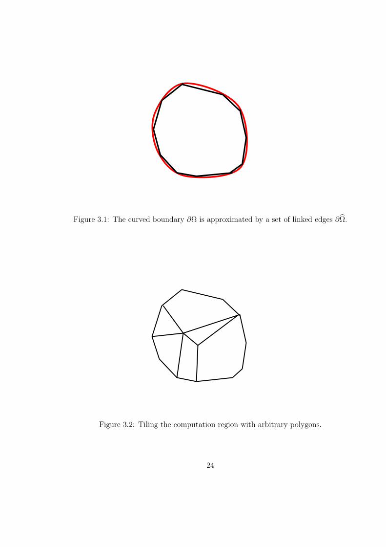
Figure 3.1: The curved boundary ∂Ω is approximated by a set of linked edges ∂Ω.

Figure 3.2: Tiling the computation region with arbitrary polygons.

24

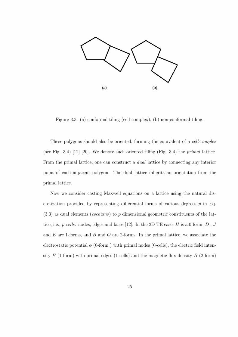
Figure 3.3: (a) conformal tiling (cell complex); (b) non-conformal tiling.

These polygons should also be oriented, forming the equivalent of a cell-complex

(see Fig. 3.4) [12] [20]. We denote such oriented tiling (Fig. 3.4) the primal lattice.

From the primal lattice, one can construct a dual lattice by connecting any interior

point of each adjacent polygon. The dual lattice inherits an orientation from the

primal lattice.

Now we consider casting Maxwell equations on a lattice using the natural dis-

cretization provided by representing differential forms of various degrees p in Eq.

(3.3) as dual elements (cochains) to p dimensional geometric constituents of the lat-

tice, i.e., p-cells : nodes, edges and faces [12]. In the 2D TE case, H is a 0-form, D , J

and E are 1-forms, and B and Q are 2-forms. In the primal lattice, we associate the

electrostatic potential φ (0-form ) with primal nodes (0-cells), the electric field inten-

sity E (1-form) with primal edges (1-cells) and the magnetic flux density B (2-form)

25

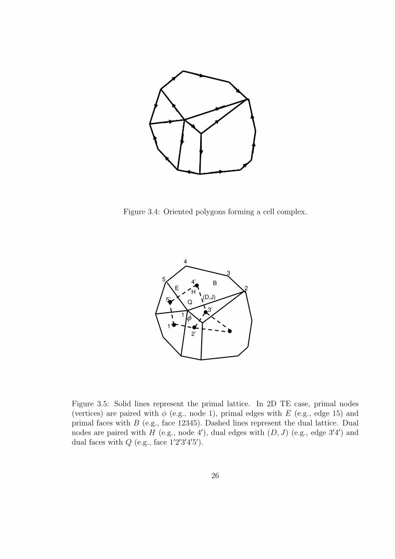
Figure 3.4: Oriented polygons forming a cell complex.

(D,J)

EB

H

5

4

3

2

1

5’

4’

2’

1’

3’

Q

Figure 3.5: Solid lines represent the primal lattice. In 2D TE case, primal nodes(vertices) are paired with φ (e.g., node 1), primal edges with E (e.g., edge 15) andprimal faces with B (e.g., face 12345). Dashed lines represent the dual lattice. Dualnodes are paired with H (e.g., node 4′), dual edges with (D, J) (e.g., edge 3′4′) anddual faces with Q (e.g., face 1′2′3′4′5′).

26

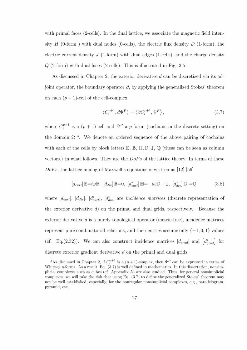
with primal faces (2-cells). In the dual lattice, we associate the magnetic field inten-

sity H (0-form ) with dual nodes (0-cells), the electric flux density D (1-form), the

electric current density J (1-form) with dual edges (1-cells), and the charge density

Q (2-form) with dual faces (2-cells). This is illustrated in Fig. 3.5.

As discussed in Chapter 2, the exterior derivative d can be discretized via its ad-

joint operator, the boundary operator ∂, by applying the generalized Stokes’ theorem

on each (p + 1)-cell of the cell-complex

⟨Cp+1

i , dΨP⟩

=⟨∂Cp+1

i , ΨP⟩, (3.7)

where Cp+1i is a (p + 1)-cell and ΨP a p-form, (cochains in the discrete setting) on

the domain Ω 3. We denote an ordered sequence of the above pairing of cochains

with each of the cells by block letters E, B, H,D, J, Q (these can be seen as column

vectors.) in what follows. They are the DoFs of the lattice theory. In terms of these

DoFs, the lattice analog of Maxwell’s equations is written as [12] [56]

[dcurl]E=iωB, [ddiv]B=0, [d∗curl]H=−iωD+ J, [d∗div]D =Q, (3.8)

where [dcurl], [ddiv], [d∗curl], [d∗div] are incidence matrices (discrete representation of

the exterior derivative d) on the primal and dual grids, respectively. Because the

exterior derivative d is a purely topological operator (metric-free), incidence matrices

represent pure combinatorial relations, and their entries assume only −1, 0, 1 values

(cf. Eq.(2.32)). We can also construct incidence matrices [dgrad] and[d∗grad

]for

discrete exterior gradient derivative d on the primal and dual grids.

3As discussed in Chapter 2, if Cp+1i is a (p + 1)-simplex, then ΨP can be expressed in terms of

Whitney p-forms. As a result, Eq. (3.7) is well defined in mathematics. In this dissertation, nonsim-plicial complexes such as cubes (cf. Appendix A) are also studied. Thus, for general nonsimplicialcomplexes, we will take the risk that using Eq. (3.7) to define the generalized Stokes’ theorem maynot be well established, especially, for the nonregular nonsimplicial complexes, e.g., parallelogram,pyramid, etc.

27

7

6

5

4

3

1

2

8

Figure 3.6: Oriented lattice.

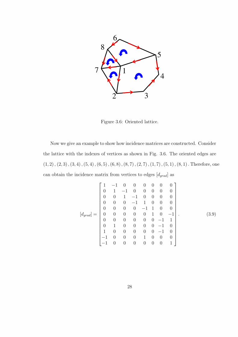
Now we give an example to show how incidence matrices are constructed. Consider

the lattice with the indexes of vertices as shown in Fig. 3.6. The oriented edges are

(1, 2) , (2, 3) , (3, 4) , (5, 4) , (6, 5) , (6, 8) , (8, 7) , (2, 7) , (1, 7) , (5, 1) , (8, 1) . Therefore, one

can obtain the incidence matrix from vertices to edges [dgrad] as

[dgrad] =

1 −1 0 0 0 0 0 00 1 −1 0 0 0 0 00 0 1 −1 0 0 0 00 0 0 −1 1 0 0 00 0 0 0 −1 1 0 00 0 0 0 0 1 0 −10 0 0 0 0 0 −1 10 1 0 0 0 0 −1 01 0 0 0 0 0 −1 0−1 0 0 0 1 0 0 0−1 0 0 0 0 0 0 1

. (3.9)

28

After setting the polygons (1, 2, 3, 4, 5) , (1, 5, 6, 8) , (1, 8, 7) , (1, 7, 2), one can similarly

obtain the incidence from edges to polygons [dcurl] as

[dcurl] =

1 1 1 −1 0 0 0 0 0 1 00 0 0 0 −1 1 0 0 0 −1 10 0 0 0 0 0 1 0 −1 0 −1−1 0 0 0 0 0 0 −1 1 0 0

. (3.10)

For 3D, the primal lattice is a network of polyhedra, and the corresponding dual

lattice can be constructed similar to 2D as discussed before. In the primal lattice,

we associate the electrostatic potential φ (0-form) with primal nodes (0-cells), the

electric field intensity E (1-form) with primal edges (1-cells) and the magnetic flux

density B (2-form) with primal faces (2-cells). In the dual lattice, we associate the

magnetic field intensity H (1-form) with dual edges (1-cells), the electric flux density

D (2-form) and the electric current density J (2 -form) with dual faces (2-cells), and

the charge density Q (3-form) with dual volumes (3-cells).

3.3 Discrete Hodge operators

The discrete constitutive equations can be, in general, written as follows

D = [?ε]E, H = [?µ−1 ]B. (3.11)

The matrices [?ε] and [?µ−1 ] are denoted as discrete Hodge operators. The construction

of discrete Hodge operators depends on the particular finite methods. In the following,

we will discuss two well defined discrete Hodge operators, Yee Hodges and Galerkin

Hodges, used for finite differences and finite elements, respectively.

3.3.1 Yee Hodges

In Cartesian coordinates, the electric field intensity 1-form E reads

E = Exdx + Eydy + Ezdz. (3.12)

29

The Hodge operator ?ε acting on E gives an electric flux 2-form D

D = ?εE = εExdy ∧ dz + εEydz ∧ dx + εEzdx ∧ dy. (3.13)

In addition, the magnetic field flux 2-form B reads

B = Bxdy ∧ dz + Bydz ∧ dx + Bzdx ∧ dy. (3.14)

Hodge operator ?µ−1 acting on B gives magnetic field intensity 1-form H

H = ?µ−1B =1

µBxdx +

1

µBydy +

1

µBzdz. (3.15)

We consider a regular hexahedral lattice ∆x = ∆y = ∆z = L. The discrete field

physical quantities can be defined on the lattice. That is, the electrical field intensity

E is defined on edges (e.g., Ex∆x), the magnetic flux intensity B defined on faces

(e.g., Bz∆x∆y), and the electrical flux intensity D is defined on dual faces (e.g.,

Dx∆y∆z), the magnetic field intensity H defined on dual edges (e.g., Hz∆z). The

Yee discrete Hodge is obtained by replacing the infinitesimal dx, dy, dz with lattice

elements ∆x, ∆y, ∆z. Let E (i) = Ex (i) ∆x be the electrical field intensity (discrete

1-form) E at edge i. Hodge operator ?ε acting on E (i) gives D (i) via

D (i) = ?εE (i) = ?εEx (i) ∆x. (3.16)

The corresponding electrical flux intensity (discrete 2-form) D (i) also reads

D (i) = Dx (i) ∆y∆z = εEx (i) ∆y∆z. (3.17)

Comparison of Eq.(3.16) and Eq.(3.17) gives [?ε]i,i = εL . On the Yee’s lattice,

when i 6= j, assume [?ε]i,j = 0 . A general entry of Yee Hodge matrix [?ε] reads as

[?ε]i,j = εLδi,j. (3.18)

30

Similarly, we obtain a general entry of Yee Hodge matrix [?µ−1 ]

[?µ−1 ]i,j =1

µLδi,j. (3.19)

Note that Yee Hodge matrices [?ε] and [?µ−1 ] are diagonal matrices.

3.3.2 Galerkin Hodges

As discussed in Ch. 2, one can use Poincare duality (contraction) to define a

Hodge star operator ? in n-dimensional space. For some form Ψp, the Hodge square

of Ψp is defined as

(Ψp, Ψp) =

∫

Ω

Ψp ∧ ?Ψp, (3.20)

which is positive when the metric is positive definite. By applying (3.20) to the

electric field and magnetic field, one can obtain constitutive relations in terms of

Hodge operators in 3D Euclidean space R3 as

(E, E) =

∫

R3

E ∧D =

∫

R3

E ∧ ?εE, (3.21)

(B, B) =

∫

R3

B ∧H =

∫

R3

B ∧ ?µ−1B. (3.22)

As also discussed in Chapter 2, Whitney forms [27] are the basic interpolants for

discrete differential forms of various degrees defined over tetrahedra. Whitney forms

can be expressed in term of the barycentric coordinates (ζi, ζj, ζk, ζr) associated with

each tetrahedron nodes (i, j, k, r) as [48]

w0i = ζi, (3.23)

w1i,j = ζidζj − ζjdζi, (3.24)

w2i,j,k = 2 (ζidζj ∧ dζk + ζjdζk ∧ dζi + ζkdζi ∧ dζj) , (3.25)

w3i,j,k,r = 6

(ζidζj ∧ dζk ∧ dζr − ζrdζi ∧ dζj ∧ dζk

+ζkdζr ∧ dζi ∧ dζj − ζjdζk ∧ dζr ∧ dζi

). (3.26)

31

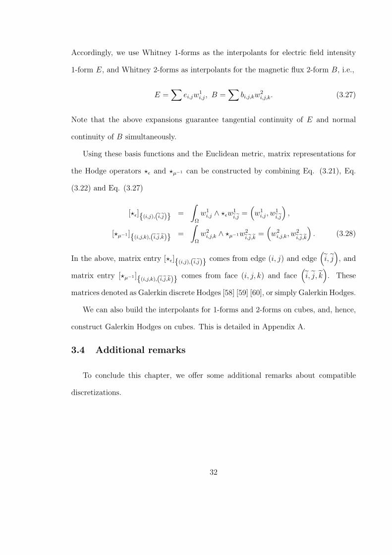
Accordingly, we use Whitney 1-forms as the interpolants for electric field intensity

1-form E, and Whitney 2-forms as interpolants for the magnetic flux 2-form B, i.e.,

E =∑

ei,jw1i,j, B =

∑bi,j,kw

2i,j,k. (3.27)

Note that the above expansions guarantee tangential continuity of E and normal

continuity of B simultaneously.

Using these basis functions and the Euclidean metric, matrix representations for

the Hodge operators ?ε and ?µ−1 can be constructed by combining Eq. (3.21), Eq.

(3.22) and Eq. (3.27)

[?ε](i,j),(ei,ej) =

∫

Ω

w1i,j ∧ ?εw

1ei,ej =

(w1

i,j, w1ei,ej

),

[?µ−1 ](i,j,k),(ei,ej,ek) =

∫

Ω

w2i,j,k ∧ ?µ−1w2

ei,ej,ek =(w2

i,j,k, w2ei,ej,ek

). (3.28)

In the above, matrix entry [?ε](i,j),(ei,ej) comes from edge (i, j) and edge(i, j

), and

matrix entry [?µ−1 ](i,j,k),(ei,ej,ek) comes from face (i, j, k) and face(i, j, k

). These

matrices denoted as Galerkin discrete Hodges [58] [59] [60], or simply Galerkin Hodges.

We can also build the interpolants for 1-forms and 2-forms on cubes, and, hence,

construct Galerkin Hodges on cubes. This is detailed in Appendix A.

3.4 Additional remarks

To conclude this chapter, we offer some additional remarks about compatible

discretizations.

32

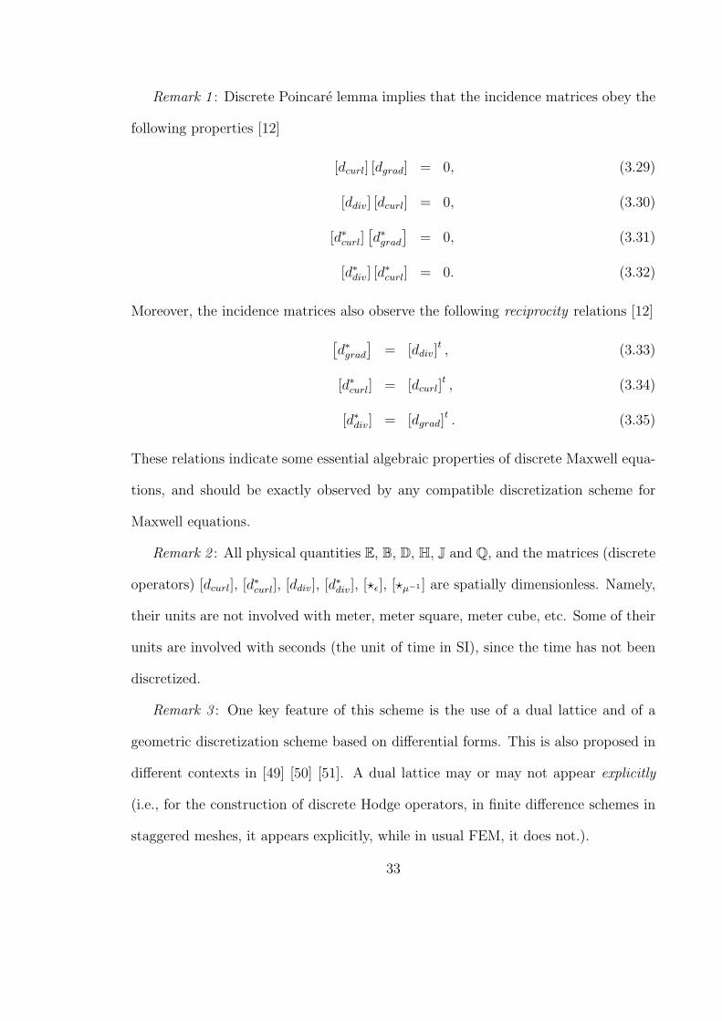
Remark 1 : Discrete Poincare lemma implies that the incidence matrices obey the

following properties [12]

[dcurl] [dgrad] = 0, (3.29)

[ddiv] [dcurl] = 0, (3.30)

[d∗curl][d∗grad

]= 0, (3.31)

[d∗div] [d∗curl] = 0. (3.32)

Moreover, the incidence matrices also observe the following reciprocity relations [12]

[d∗grad

]= [ddiv]

t , (3.33)

[d∗curl] = [dcurl]t , (3.34)

[d∗div] = [dgrad]t . (3.35)

These relations indicate some essential algebraic properties of discrete Maxwell equa-

tions, and should be exactly observed by any compatible discretization scheme for

Maxwell equations.

Remark 2 : All physical quantities E, B, D, H, J and Q, and the matrices (discrete

operators) [dcurl], [d∗curl], [ddiv], [d∗div], [?ε], [?µ−1 ] are spatially dimensionless. Namely,

their units are not involved with meter, meter square, meter cube, etc. Some of their

units are involved with seconds (the unit of time in SI), since the time has not been

discretized.

Remark 3 : One key feature of this scheme is the use of a dual lattice and of a

geometric discretization scheme based on differential forms. This is also proposed in

different contexts in [49] [50] [51]. A dual lattice may or may not appear explicitly

(i.e., for the construction of discrete Hodge operators, in finite difference schemes in

staggered meshes, it appears explicitly, while in usual FEM, it does not.).

33

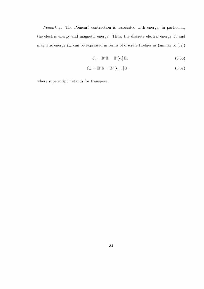
Remark 4 : The Poincare contraction is associated with energy, in particular,

the electric energy and magnetic energy. Thus, the discrete electric energy Ee and

magnetic energy Em can be expressed in terms of discrete Hodges as (similar to [52])

Ee = DtE = Et[?ε]E, (3.36)

Em = HtB = Bt [?µ−1 ]B, (3.37)

where superscript t stands for transpose.

34

CHAPTER 4

DISCRETE HODGE DECOMPOSITION

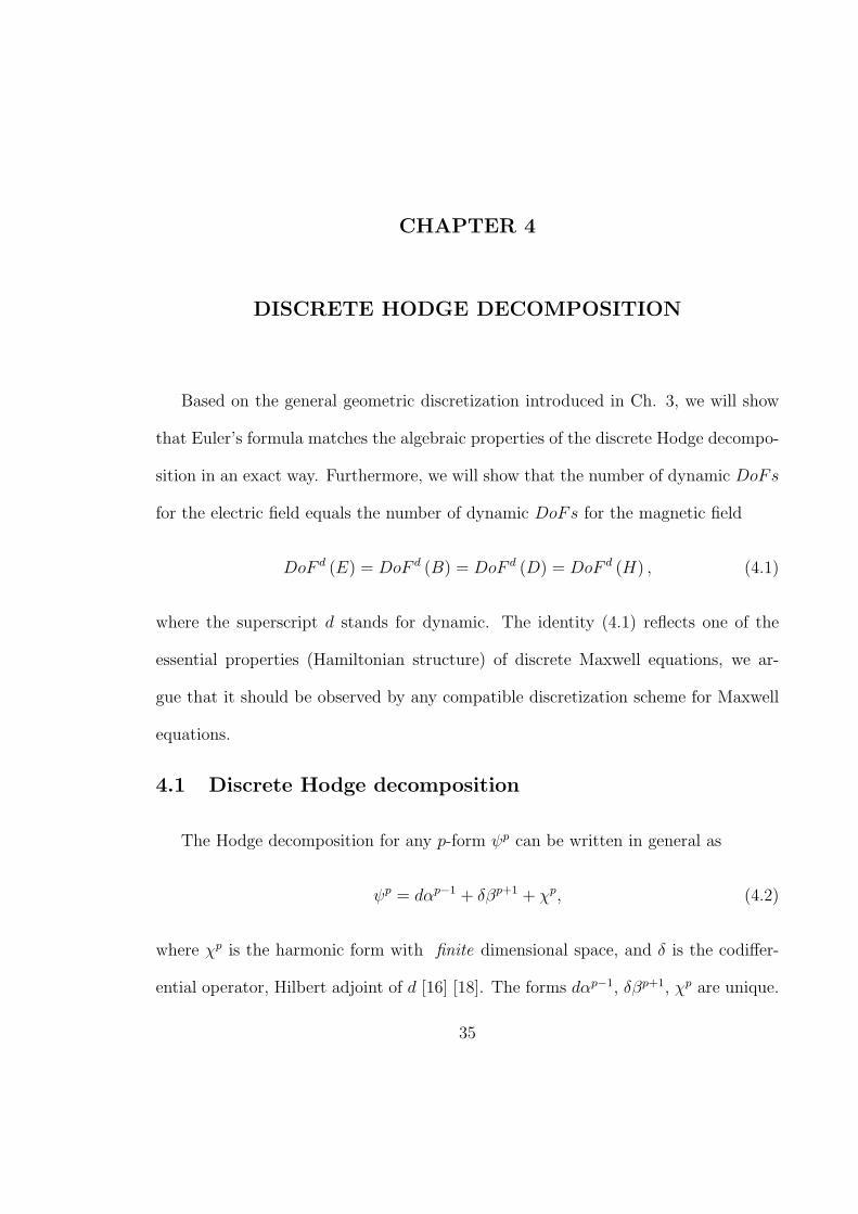
Based on the general geometric discretization introduced in Ch. 3, we will show

that Euler’s formula matches the algebraic properties of the discrete Hodge decompo-

sition in an exact way. Furthermore, we will show that the number of dynamic DoFs

for the electric field equals the number of dynamic DoFs for the magnetic field

DoF d (E) = DoF d (B) = DoF d (D) = DoF d (H) , (4.1)

where the superscript d stands for dynamic. The identity (4.1) reflects one of the

essential properties (Hamiltonian structure) of discrete Maxwell equations, we ar-

gue that it should be observed by any compatible discretization scheme for Maxwell

equations.

4.1 Discrete Hodge decomposition

The Hodge decomposition for any p-form ψp can be written in general as

ψp = dαp−1 + δβp+1 + χp, (4.2)

where χp is the harmonic form with finite dimensional space, and δ is the codiffer-

ential operator, Hilbert adjoint of d [16] [18]. The forms dαp−1, δβp+1, χp are unique.

35

Applying (4.2) to the electric field intensity 1-form E, we obtain

E = dφ + δA + χ, (4.3)

where φ is a 0-form and A is a 2-form. In Eq. (4.3) dφ represents the static field,

δA represents the dynamic field, and χ represents the harmonic field component (if

any).

4.1.1 2+1 theory in a contractible domain

If domain Ω is contractible, χ is identically zero and the Hodge decomposition can

be simplified to

E = dφ + δA. (4.4)

In our compatible discretizations, the number of DoFs for the static field equals

the number of internal nodes of the primal lattice. This is because the DoFs of the

potential φ, which is a 0-form, are associated to nodes. This is well known in the

FEM context, e.g., [9] [53] [62]. We show next identity (4.1). The Euler’s formula for

a general network of polygons without holes (Fig. 3.2) is given by

NV −NE = 1−NF , (4.5)

where NV is the number of vertices (nodes), NE the number of edges, and NF the

number of faces (cells). For any ∂Ω, it is easy to verify that

N bV −N b

E = 0, (4.6)

where N bV is the number of vertices on the boundary and N b

E the number of edges

on the boundary (the superscript b standing for boundary). Note that cochains

on ∂Ω are not associated to DoFs, since they are fixed by boundary conditions

36

(For concreteness, we consider Dirichlet boundary conditions here). Using Hodge

decomposition (4.4), the number of dynamic (ω 6= 0 ) DoFs of the electric field,

corresponding to δA, is given by

DoF d (E) = N inE −N in

V

=(NE −N b

E

)− (NV −N b

V

)

= NE −NV , (4.7)

where the superscript in stands for internal. Since E is given along the boundary,

then, for ω 6= 0,∫bΩ B is fixed by

iω

∫bΩB =

∫

∂bΩE. (4.8)

This corresponds to one constraint on B. Subtracting one degree of freedom from

the constraint (4.8), the number dynamic DoFs of the magnetic flux B is

DoF d (B) = NF − 1. (4.9)

From Euler’s formula (4.5), we then have the identity

DoF d (E) = DoF d (B) . (4.10)

Furthermore, thanks to the Hodge isomorphism, the identity (4.1) follows directly.

4.1.2 3+1 theory in a contractible domain

The source free Maxwell equations in 3+1 dimensions read as

dE = iωB, (4.11)

dB = 0, (4.12)

dH = −iωD, (4.13)

dD = 0, (4.14)

37

where H and E are 1-forms, and D and B are 2-forms. The spatial domain Ω is

again (approximately) tiled by a set of polyhedra Ω and the boundary ∂Ω is by a

polyhedron ∂Ω . Using Euler’s formula for Ω, we have

NV −NE = 1−NF + NP , (4.15)

and Euler’s formula for the boundary polyhedron ∂Ω

N bV −N b

E = 2−N bF , (4.16)

where NP is now the number of polyhedra. Combining Eq. (4.15) and (4.16), we

obtain

(NE −N b

E

)− (NV −N b

V

)=

(NF −N b

F

)− (NP − 1) . (4.17)

Using the Hodge decomposition (4.4), the number of dynamic DoFs of the electric

field (corresponding to δA) is


V

=(NE −N b

E

)− (NV −N b

V

). (4.18)

Each polyhedron produces one constraint for the magnetic flux B from Eq.(4.12).

Furthermore, this set of constraints span the condition at the boundary ∂Ω. The

total number of the constrains for B is therefore (NP − 1) . Consequently, the number

of DoFs for the magnetic flux B is

DoF d (B) = N inF − (NP − 1)

=(NF −N b

F

)− (NP − 1) . (4.19)

Identity (4.1) then follows from Eq. (4.17), (4.18) and (4.19).

38

2

3

1

Figure 4.1: 2+1 theory in a non-contractible domain (network of polygons with ahole, illustrated by a triangle 123).

4.1.3 2+1 theory in a non-contractible domain

Now consider a non-contractible two-dimensional domain Ω with a finite number

g of holes (genus). This is illustrated in Fig. 4.1 for g = 1. Along the boundary of

each hole, the electric field E is constrained by

∫E = M, (4.20)

where the magnetic current density 4 M (passing through the hole) is a known quan-

tity. The equation (4.20) accounts for the possible existence of the harmonic forms χ

on Ω. In particular, the number of holes g is equal to the dimension of the space of

harmonic forms χ and gives the number of independent constraint equations (4.20).

4In physical terms, the magnetic current density M is identified with the “displacement magneticcurrent density” iωB, which is given for some cases. In some other cases, M may also arise fromequivalent magnetic current density by the surface equivalence theorem [63]. It should be emphasizedthat, of course, the equivalent magnetic current results from an impressed electric field E, not fromthe movement of any “magnetic charge”.

39

Subtracting g from Eq. (4.7), the number of dynamic DoFs of the electric field in

this case becomes


V − g

= NE −NV − g, (4.21)

whereas the number of DoFs of the magnetic flux DoF d (B) remains NF − 1.

Since Euler’s formula for a network of polygons with g holes is

NV −NE = (1− g)−NF , (4.22)

we have that from Eq. (4.9), (4.21) and (4.22), the identity (4.1) is again satisfied.

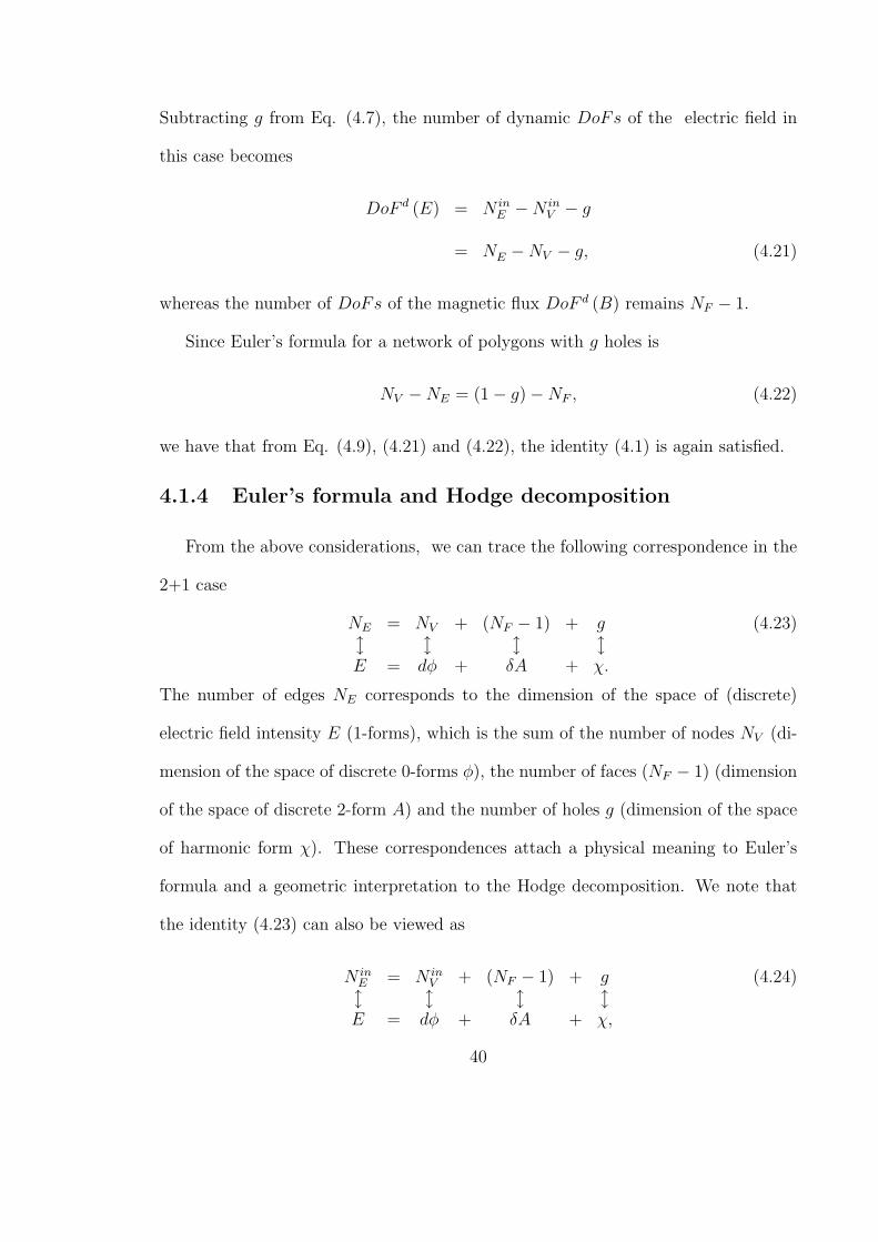
4.1.4 Euler’s formula and Hodge decomposition

From the above considerations, we can trace the following correspondence in the

2+1 case

NE = NV + (NF − 1) + gl l l lE = dφ + δA + χ.

(4.23)

The number of edges NE corresponds to the dimension of the space of (discrete)

electric field intensity E (1-forms), which is the sum of the number of nodes NV (di-

mension of the space of discrete 0-forms φ), the number of faces (NF − 1) (dimension

of the space of discrete 2-form A) and the number of holes g (dimension of the space

of harmonic form χ). These correspondences attach a physical meaning to Euler’s

formula and a geometric interpretation to the Hodge decomposition. We note that

the identity (4.23) can also be viewed as

N inE = N in

V + (NF − 1) + gl l l lE = dφ + δA + χ,

(4.24)

40

xE x

E

xE

xE

xE

xE

yEyE

yEyE

yEyE

zHzHzH

zHzHzH

zHzHzH

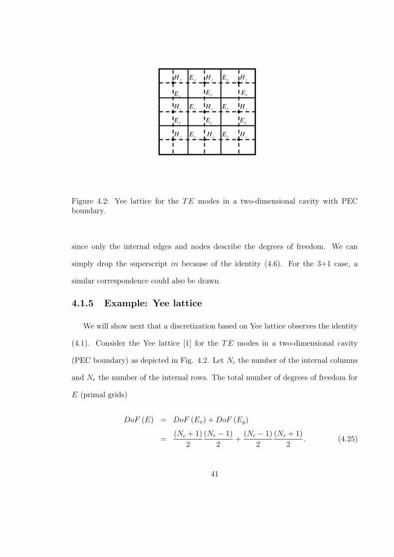
Figure 4.2: Yee lattice for the TE modes in a two-dimensional cavity with PECboundary.

since only the internal edges and nodes describe the degrees of freedom. We can

simply drop the superscript in because of the identity (4.6). For the 3+1 case, a

similar correspondence could also be drawn.

4.1.5 Example: Yee lattice

We will show next that a discretization based on Yee lattice observes the identity

(4.1). Consider the Yee lattice [1] for the TE modes in a two-dimensional cavity

(PEC boundary) as depicted in Fig. 4.2. Let Nc the number of the internal columns

and Nr the number of the internal rows. The total number of degrees of freedom for

E (primal grids)

DoF (E) = DoF (Ex) + DoF (Ey)

=(Nc + 1)

2

(Nr − 1)

2+

(Nc − 1)

2

(Nr + 1)

2. (4.25)

41

and the total number of degrees of freedom for H (dual grids) is

DoF (H) =(Nc + 1)

2

(Nr + 1)

2. (4.26)

We need to enforce the divergence free condition for the electric fields E, whose

number is

DoF (φ) =(Nc − 1)

2

(Nr − 1)

2, (4.27)

which also corresponds to the electrostatic modes by the discrete Helmholtz decom-

positions. The DoF of the dynamic electric field DoF d (E) is

DoF d (E) = DoF (E)−DoF (φ)

=(Nc + 1)

2

(Nr − 1)

2+

(Nc − 1)

2

(Nr + 1)

2

−(Nc − 1)

2

(Nr − 1)

2

=NcNr + Nc + Nr − 3

4. (4.28)

Meanwhile, the number of DoF of dynamic magnetic field DoF d (H) is

DoF d (H) = DoF (H)− 1

=(Nc + 1)

2

(Nr + 1)

2− 1

=NcNr + Nc + Nr − 3

4, (4.29)

where we subtract one degree of freedom from DoF (H) because we need to choose

a reference node for H (0-form). From the Eq. (4.28) and Eq.(4.29), Yee lattice

satisfies the identity (4.1). A similar analysis can also be applied for the 3D case.

4.2 Some local properties of the discrete Hodge decomposi-tion

We next use electrical field intensity−→E (a 1- form vector field) for a simplicial 2D

TE lattice to discuss some local properties of discrete Hodge decomposition. Inside

42

each element, the electrical field intensity−→E can be expressed, in general, as a linear

combination of the three edge elements (Whitney 1-forms) associated with the three

edges: ij, jk, ki, i.e.,

−→E = eij

−→W 1

ij + ejk−→W 1

jk + eki−→W 1

ki, (4.30)

where (eij, ejk, eki) are real coefficients.

It can be shown that the basis functions−→W 1

ij,−→W 1

jk and−→W 1

ki are in general not

orthogonal with each other. That is

⟨−→W 1

ij,−→W 1

jk

⟩6= 0, (4.31)

⟨−→W 1

jk,−→W 1

ki

⟩6= 0, (4.32)

⟨−→W 1

ki,−→W 1

ij

⟩6= 0, (4.33)

where 〈, 〉 stands for inner product, and the above inner products are defined by

Eq.(3.28) for 2D case. The vector calculus version of Hodge decomposition (also

known as Helmholtz decomposition) is

−→E =

−→∇φ +−→∇ ×−→A. (4.34)

In general, each basis function of−→W 1

ij,−→W 1

jk and−→W 1

ki is composed of the static field

−→∇φ (pure gradient field) and the dynamic field−→∇ × −→A (pure curl field). Here, we

suggest an orthogonal set of basis functions(−→

V 1,−→V 2,

−→V 3

)to express electrical field

intensity−→E

−→E = v1

−→V 1 + v2

−→V 2 + v3

−→V 3. (4.35)

43

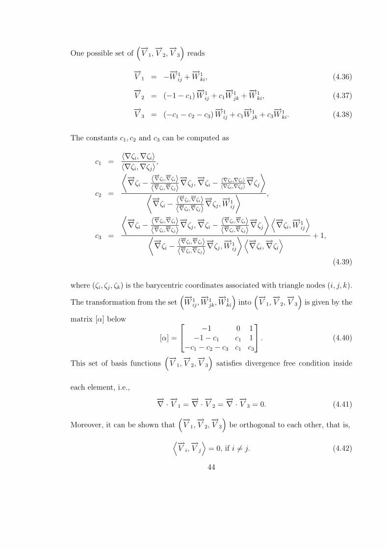
One possible set of(−→

V 1,−→V 2,

−→V 3

)reads

−→V 1 = −−→W 1

ij +−→W 1

ki, (4.36)

−→V 2 = (−1− c1)

−→W 1

ij + c1−→W 1

jk +−→W 1

ki, (4.37)

−→V 3 = (−c1 − c2 − c3)

−→W 1

ij + c1−→W 1

jk + c3−→W 1

ki. (4.38)

The constants c1, c2 and c3 can be computed as

c1 =〈∇ζi,∇ζi〉〈∇ζi,∇ζj〉 ,

c2 =

⟨−→∇ζi − 〈−→∇ζi,−→∇ζi〉

〈−→∇ζi,−→∇ζj〉

−→∇ζj,−→∇ζi − 〈∇ζi,∇ζi〉

〈∇ζi,∇ζj〉−→∇ζj

⟩

⟨−→∇ζi − 〈−→∇ζi,−→∇ζi〉

〈−→∇ζi,−→∇ζj〉

−→∇ζj,−→W 1

ij

⟩ ,

c3 =

⟨−→∇ζi − 〈−→∇ζi,−→∇ζi〉

〈−→∇ζi,−→∇ζj〉

−→∇ζj,−→∇ζi − 〈−→∇ζi,

−→∇ζi〉〈−→∇ζi,

−→∇ζj〉−→∇ζj

⟩ ⟨−→∇ζi,−→W 1

ij

⟩

⟨−→∇ζi − 〈−→∇ζi,−→∇ζi〉

〈−→∇ζi,−→∇ζj〉

−→∇ζj,−→W 1

ij

⟩ ⟨−→∇ζi,−→∇ζi

⟩ + 1,

(4.39)

where (ζi, ζj, ζk) is the barycentric coordinates associated with triangle nodes (i, j, k).

The transformation from the set(−→W 1

ij,−→W 1

jk,−→W 1

ki

)into

(−→V 1,

−→V 2,

−→V 3

)is given by the

matrix [α] below

[α] =

−1 0 1−1− c1 c1 1

−c1 − c2 − c3 c1 c3

. (4.40)

This set of basis functions(−→

V 1,−→V 2,

−→V 3

)satisfies divergence free condition inside

each element, i.e.,

−→∇ · −→V 1 =−→∇ · −→V 2 =

−→∇ · −→V 3 = 0. (4.41)

Moreover, it can be shown that(−→

V 1,−→V 2,

−→V 3

)be orthogonal to each other, that is,

⟨−→V i,

−→V j

⟩= 0, if i 6= j. (4.42)

44

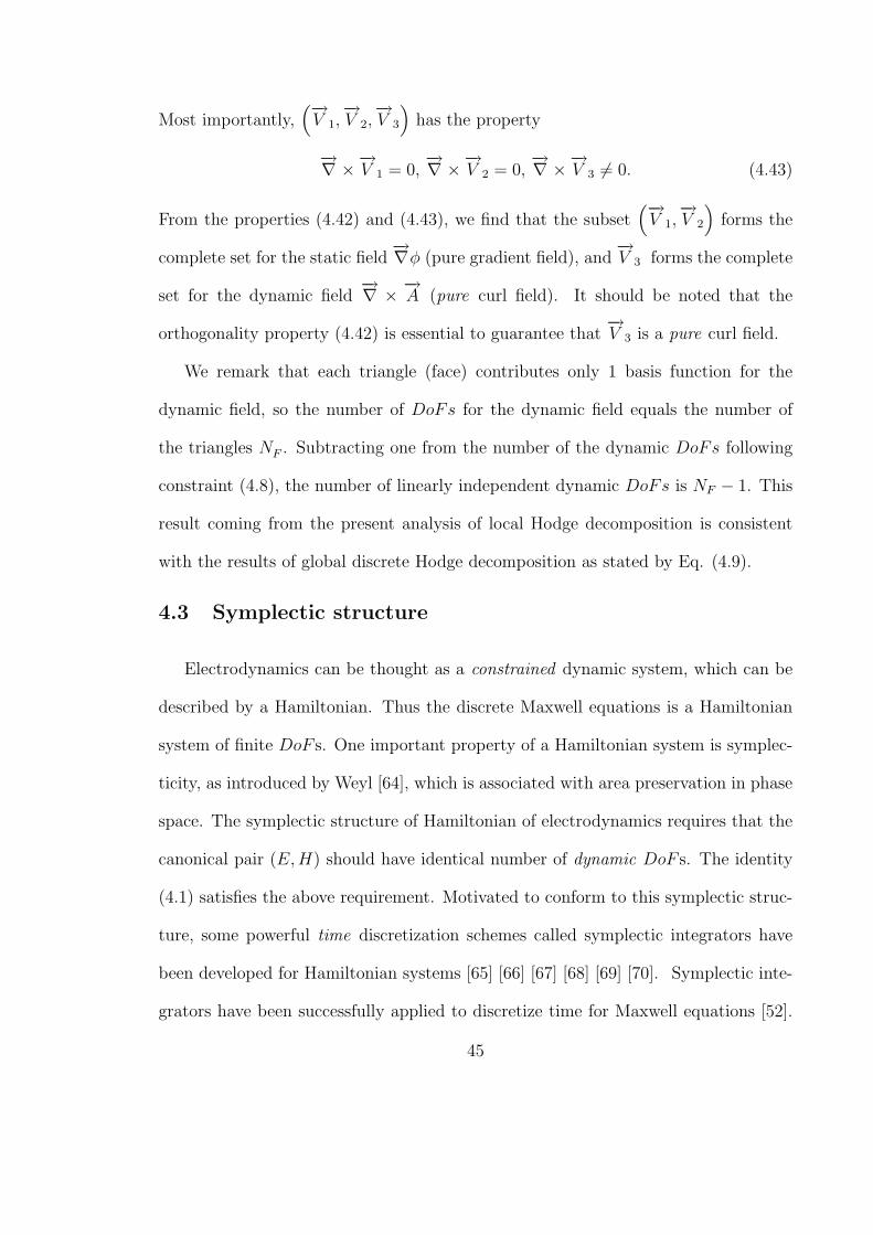
Most importantly,(−→

V 1,−→V 2,

−→V 3

)has the property

−→∇ ×−→V 1 = 0,−→∇ ×−→V 2 = 0,

−→∇ ×−→V 3 6= 0. (4.43)

From the properties (4.42) and (4.43), we find that the subset(−→

V 1,−→V 2

)forms the

complete set for the static field−→∇φ (pure gradient field), and

−→V 3 forms the complete

set for the dynamic field−→∇ × −→

A (pure curl field). It should be noted that the

orthogonality property (4.42) is essential to guarantee that−→V 3 is a pure curl field.

We remark that each triangle (face) contributes only 1 basis function for the

dynamic field, so the number of DoFs for the dynamic field equals the number of

the triangles NF . Subtracting one from the number of the dynamic DoFs following

constraint (4.8), the number of linearly independent dynamic DoFs is NF − 1. This

result coming from the present analysis of local Hodge decomposition is consistent

with the results of global discrete Hodge decomposition as stated by Eq. (4.9).

4.3 Symplectic structure

Electrodynamics can be thought as a constrained dynamic system, which can be

described by a Hamiltonian. Thus the discrete Maxwell equations is a Hamiltonian

system of finite DoF s. One important property of a Hamiltonian system is symplec-

ticity, as introduced by Weyl [64], which is associated with area preservation in phase

space. The symplectic structure of Hamiltonian of electrodynamics requires that the

canonical pair (E, H) should have identical number of dynamic DoF s. The identity

(4.1) satisfies the above requirement. Motivated to conform to this symplectic struc-

ture, some powerful time discretization schemes called symplectic integrators have

been developed for Hamiltonian systems [65] [66] [67] [68] [69] [70]. Symplectic inte-

grators have been successfully applied to discretize time for Maxwell equations [52].

45

However, it has been thought that symplectic integration is not entirely consistent

with discrete Maxwell equations since DoF (E) 6= DoF (H) [52]. The fact that dis-

crete Maxwell equations satisfy DoF d (E) = DoF d (H) as explained above provides

a simple explanation to this apparent dilemma.


To conclude this chapter, we offer some additional remarks.

Remark 1 : For the case of high order 1-forms, the DoFs of 1-forms can be associ-

ated with the faces and volumes [71]. Nevertheless, following the de Rham diagram,

the dimension of the range space of 1-forms (e.g., E) equals the null space of 2-forms

(e.g., B), so the identity (4.1) still holds.

Remark 2 : The identity (4.1) is violated by some common finite difference tech-

niques such as those utilizing subgridding schemes. Violation of the identity (4.1)

may provide a possible fundamental explanation why some subgridding schemes are

not (late-time) stable (non compatible).

Remark 3 : The Hodge decomposition is a generalization of Helmholtz decompo-

sition. For a brief history of Helmholtz decomposition and Hodge decomposition,

see [72]. The application of Hodge decomposition to computational electromagnetics

was pioneered by Kotiuga [73].

46

CHAPTER 5

FEM IN PRIMAL AND DUAL SPACES: GALERKINDUALITY

The basic strategy of traditional FEM (Galerkin’s method) is to seek the solu-

tion by weighting the residual of the second-order wave equations [3] [4]. Here, we

adopt a different route to derive FEM schemes. Based on the compatible discretiza-

tion schemes for Maxwell equations on irregular lattices described in Chapter 3 and

using Galerkin Hodges, we construct two system matrices in terms of the electric

field intensity E (denoted as primal formulation) and the magnetic field intensity H

(denoted as dual formulation), respectively. The primal formulation exactly recovers

the FEM based on edge elements, and suggests a geometric foundation for it. On

the other hand, the dual formulation suggests a new (dual) type of FEM. Although

both formulations give identical physical solutions, the dimensions of the null spaces

are different. The connection between the primal formulation and dual formulation

is established via a transformation denoted here as Galerkin duality. Algebraic rela-

tionships among the DoFs of primal and dual FEM formulations are explained using

a discrete version of the Hodge decomposition and Euler’s formula for a network of

polygons for 2D case and polyhedra for 3D case.

47

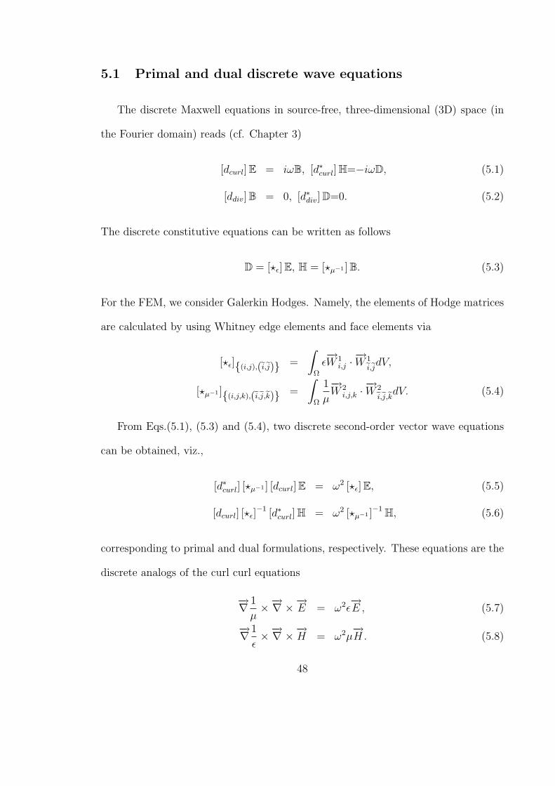
5.1 Primal and dual discrete wave equations

The discrete Maxwell equations in source-free, three-dimensional (3D) space (in

the Fourier domain) reads (cf. Chapter 3)

[dcurl]E = iωB, [d∗curl]H=−iωD, (5.1)

[ddiv]B = 0, [d∗div]D=0. (5.2)

The discrete constitutive equations can be written as follows

D = [?ε]E, H = [?µ−1 ]B. (5.3)

For the FEM, we consider Galerkin Hodges. Namely, the elements of Hodge matrices

are calculated by using Whitney edge elements and face elements via

[?ε](i,j),(ei,ej) =

∫

Ω

ε−→W 1

i,j ·−→W 1ei,ejdV,

[?µ−1 ](i,j,k),(ei,ej,ek) =

∫

Ω

1

µ

−→W 2

i,j,k ·−→W 2ei,ej,ekdV. (5.4)

From Eqs.(5.1), (5.3) and (5.4), two discrete second-order vector wave equations

can be obtained, viz.,

[d∗curl] [?µ−1 ] [dcurl]E = ω2 [?ε]E, (5.5)

[dcurl] [?ε]−1 [d∗curl]H = ω2 [?µ−1 ]−1H, (5.6)

corresponding to primal and dual formulations, respectively. These equations are the

discrete analogs of the curl curl equations

−→∇ 1

µ×−→∇ ×−→E = ω2ε

−→E , (5.7)

−→∇ 1

ε×−→∇ ×−→H = ω2µ

−→H. (5.8)

48

It is important to note that this does not imply that both Eq. (5.5) and Eq. (5.6)

simply correspond to edge element discretization of Eq. (5.7) and Eq. (5.8) in the

FEM mesh (primal lattice). Eq. (5.5) does indeed corresponds to the edge element

discretization of Eq. (5.7) in primal lattice. However, Eq. (5.6) corresponds to the

discretization of Eq. (5.8) on the dual lattice. Indeed, from the Hodge isomorphism

between B and H, the DoFs of H are associated with faces (not edges) of the FEM

mesh. Also note that the primal lattice is simplicial, but dual lattice is not simplicial

anymore. It will be shown (in Section 5.2 for 2D cases and Appendix A for 3D cases)

that [d∗curl] [?µ−1 ] [dcurl] is identical to the conventional stiffness matrix [S], arising in

FEM using edge elements

[S](i,j),(ei,ej) =

∫1

µ

(−→∇ ×−→W 1i,j

)·(−→∇ ×−→W 1

ei,ej

)dV. (5.9)

Moreover, the Hodge matrix [?ε] is identical to the conventional mass matrix. Hence,

the primal formulation recovers the conventional edge-element FEM and suggests a

geometric foundation for it. For the dual formulation, we can similarly define dual

stiffness[S†

]and mass

[M †] matrices

[S†

]= [dcurl] [?ε]

−1 [d∗curl] , (5.10)

[M †] = [?µ−1 ]−1 . (5.11)

However, this dual formulation has no direct counterpart in traditional FEM. As

discussed Section 5.3, these two formulations lead to the same dynamic solutions, but

have different mathematical properties.

49

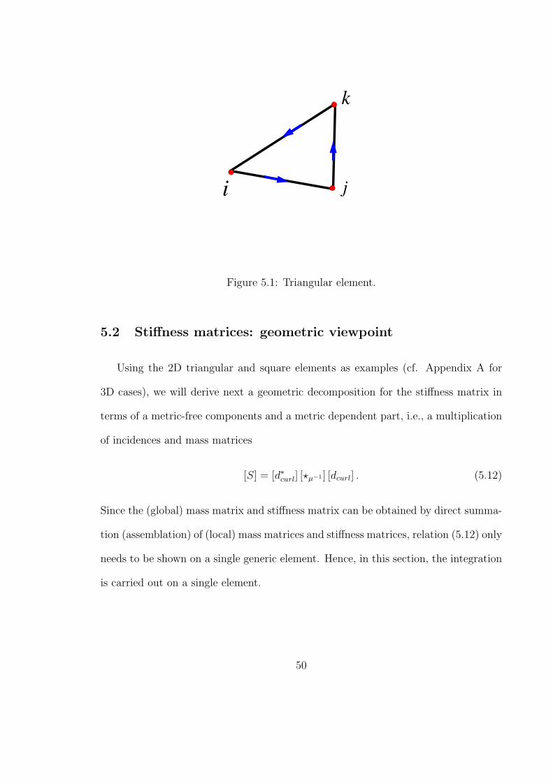
i

k

j

Figure 5.1: Triangular element.

5.2 Stiffness matrices: geometric viewpoint

Using the 2D triangular and square elements as examples (cf. Appendix A for

3D cases), we will derive next a geometric decomposition for the stiffness matrix in

terms of a metric-free components and a metric dependent part, i.e., a multiplication

of incidences and mass matrices

[S] = [d∗curl] [?µ−1 ] [dcurl] . (5.12)

Since the (global) mass matrix and stiffness matrix can be obtained by direct summa-

tion (assemblation) of (local) mass matrices and stiffness matrices, relation (5.12) only

needs to be shown on a single generic element. Hence, in this section, the integration

is carried out on a single element.

50

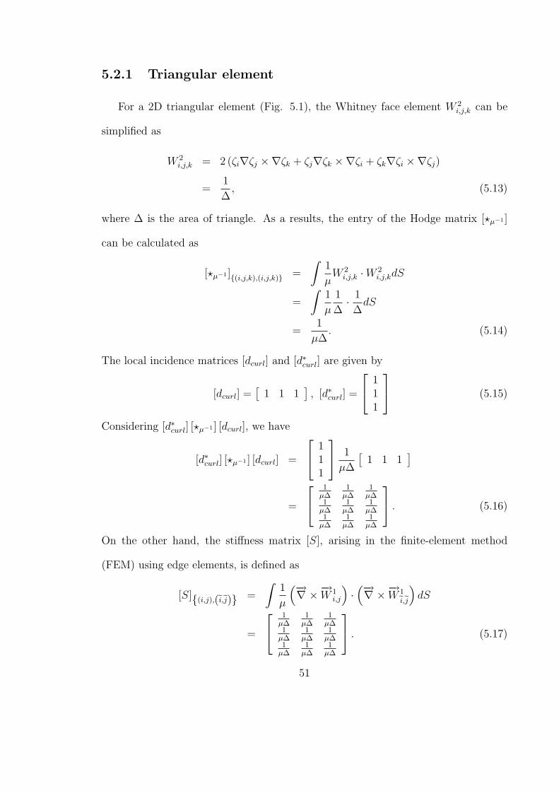
5.2.1 Triangular element

For a 2D triangular element (Fig. 5.1), the Whitney face element W 2i,j,k can be

simplified as

W 2i,j,k = 2 (ζi∇ζj ×∇ζk + ζj∇ζk ×∇ζi + ζk∇ζi ×∇ζj)

=1

∆, (5.13)

where ∆ is the area of triangle. As a results, the entry of the Hodge matrix [?µ−1 ]

can be calculated as

[?µ−1 ](i,j,k),(i,j,k) =

∫1

µW 2

i,j,k ·W 2i,j,kdS

=

∫1

µ

1

∆· 1

∆dS

=1

µ∆. (5.14)

The local incidence matrices [dcurl] and [d∗curl] are given by

[dcurl] =[

1 1 1], [d∗curl] =

111

(5.15)

Considering [d∗curl] [?µ−1 ] [dcurl], we have

[d∗curl] [?µ−1 ] [dcurl] =

111

1

µ∆

[1 1 1

]

=

1µ∆

1µ∆

1µ∆

1µ∆

1µ∆

1µ∆

1µ∆

1µ∆

1µ∆

. (5.16)

On the other hand, the stiffness matrix [S], arising in the finite-element method

(FEM) using edge elements, is defined as

[S](i,j),(ei,ej) =

∫1

µ

(−→∇ ×−→W 1i,j

)·(−→∇ ×−→W 1

ei,ej

)dS

=

1µ∆

1µ∆

1µ∆

1µ∆

1µ∆

1µ∆

1µ∆

1µ∆

1µ∆

. (5.17)

51

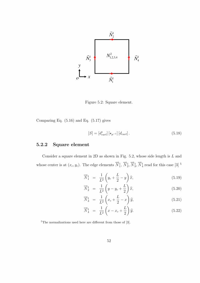
1

1N

1

2N

1

3N 1

4N

2

4,3,2,1N

x

y

o

Figure 5.2: Square element.

Comparing Eq. (5.16) and Eq. (5.17) gives

[S] = [d∗curl] [?µ−1 ] [dcurl] . (5.18)

5.2.2 Square element

Consider a square element in 2D as shown in Fig. 5.2, whose side length is L and

whose center is at (xc, yc). The edge elements−→N 1

1,−→N 1

2,−→N 1

3,−→N 1

4 read for this case [3] 5

−→N 1

1 =1

L2

(yc +

L

2− y

)x, (5.19)

−→N 1

2 =1

L2

(y − yc +

L

2

)x, (5.20)

−→N 1

3 =1

L2

(xc +

L

2− x

)y, (5.21)

−→N 1

4 =1

L2

(x− xc +

L

2

)y. (5.22)

5The normalizations used here are different from those of [3].

52

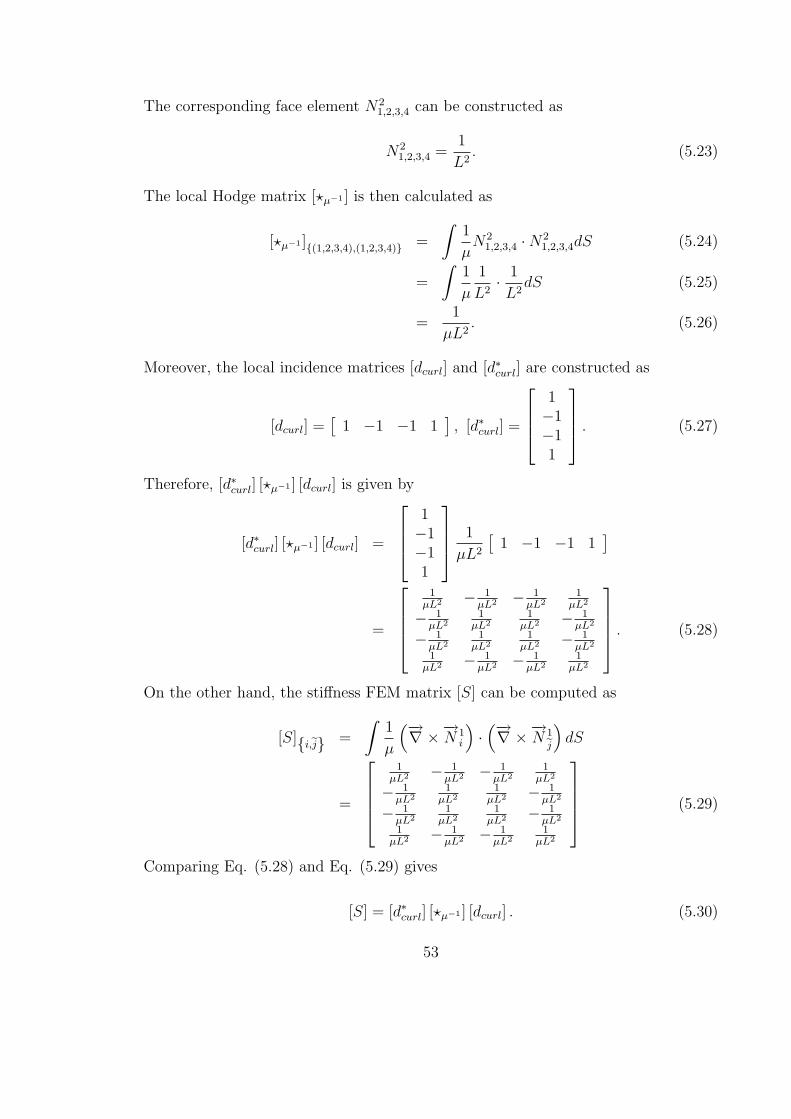
The corresponding face element N21,2,3,4 can be constructed as

N21,2,3,4 =

1

L2. (5.23)

The local Hodge matrix [?µ−1 ] is then calculated as

[?µ−1 ](1,2,3,4),(1,2,3,4) =

∫1

µN2

1,2,3,4 ·N21,2,3,4dS (5.24)

=

∫1

µ

1

L2· 1

L2dS (5.25)

=1

µL2. (5.26)

Moreover, the local incidence matrices [dcurl] and [d∗curl] are constructed as

[dcurl] =[

1 −1 −1 1], [d∗curl] =

1−1−11

. (5.27)

Therefore, [d∗curl] [?µ−1 ] [dcurl] is given by

[d∗curl] [?µ−1 ] [dcurl] =

1−1−11

1

µL2

[1 −1 −1 1

]

=

1µL2 − 1

µL2 − 1µL2

1µL2

− 1µL2

1µL2

1µL2 − 1

µL2

− 1µL2

1µL2

1µL2 − 1

µL2

1µL2 − 1

µL2 − 1µL2

1µL2

. (5.28)

On the other hand, the stiffness FEM matrix [S] can be computed as

[S]i,ej =

∫1

µ

(−→∇ ×−→N 1i

)·(−→∇ ×−→N 1

ej

)dS

=

1µL2 − 1

µL2 − 1µL2

1µL2

− 1µL2

1µL2

1µL2 − 1

µL2

− 1µL2

1µL2

1µL2 − 1

µL2

1µL2 − 1

µL2 − 1µL2

1µL2

(5.29)

Comparing Eq. (5.28) and Eq. (5.29) gives

[S] = [d∗curl] [?µ−1 ] [dcurl] . (5.30)

53

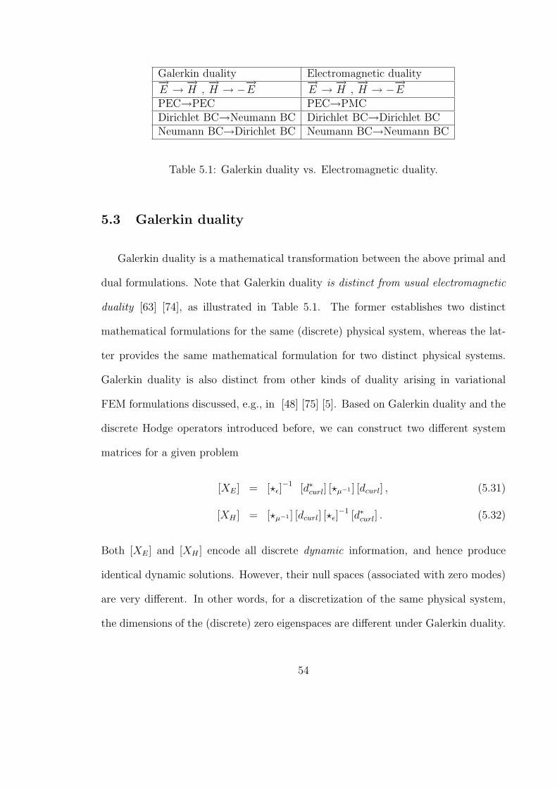
Galerkin duality Electromagnetic duality−→E → −→

H ,−→H → −−→E −→

E → −→H ,

−→H → −−→E

PEC→PEC PEC→PMCDirichlet BC→Neumann BC Dirichlet BC→Dirichlet BCNeumann BC→Dirichlet BC Neumann BC→Neumann BC

Table 5.1: Galerkin duality vs. Electromagnetic duality.

5.3 Galerkin duality

Galerkin duality is a mathematical transformation between the above primal and

dual formulations. Note that Galerkin duality is distinct from usual electromagnetic

duality [63] [74], as illustrated in Table 5.1. The former establishes two distinct

mathematical formulations for the same (discrete) physical system, whereas the lat-

ter provides the same mathematical formulation for two distinct physical systems.

Galerkin duality is also distinct from other kinds of duality arising in variational

FEM formulations discussed, e.g., in [48] [75] [5]. Based on Galerkin duality and the

discrete Hodge operators introduced before, we can construct two different system

matrices for a given problem

[XE] = [?ε]−1 [d∗curl] [?µ−1 ] [dcurl] , (5.31)

[XH ] = [?µ−1 ] [dcurl] [?ε]−1 [d∗curl] . (5.32)

Both [XE] and [XH ] encode all discrete dynamic information, and hence produce

identical dynamic solutions. However, their null spaces (associated with zero modes)

are very different. In other words, for a discretization of the same physical system,

the dimensions of the (discrete) zero eigenspaces are different under Galerkin duality.

54

This can be explained by algebraic properties of discrete Hodge decomposition, and

verified by numerical simulations, as discussed in Section 5.5 ahead.

5.4 An approach to handle Neumann boundary conditions

Since Dirichlet and Neumann boundary conditions are Galerkin dual to each other

for some underlying differential equations, Neumann boundary conditions can be

handled as follows. Consider a differential equation

Θφ = 0, (5.33)

where Θ is a differential operator and φ is the unknown physical quantity, with

Neumann boundary condition. By Galerkin duality, this problem is equivalent to

solving

Θ†φ† = 0, (5.34)

with Dirichlet boundary condition. Here Θ† is the Galerkin dual to Θ, and φ† is

the Galerkin dual to φ. Note that by using Galerkin duality, we can transform Eq.

(5.33) into Eq. (5.34), since it may be much easier to handle Dirichlet boundary

conditions than Neumann boundary conditions in some problems. The function φ†

can be expanded in terms of basis functions W †i (e.g., Whitney forms) as

φ† =∑

φ†iW†i . (5.35)

5.5 Galerkin duality: Examples

To illustrate the Galerkin duality, we provide numerical simulations of some cavity

problems.

55

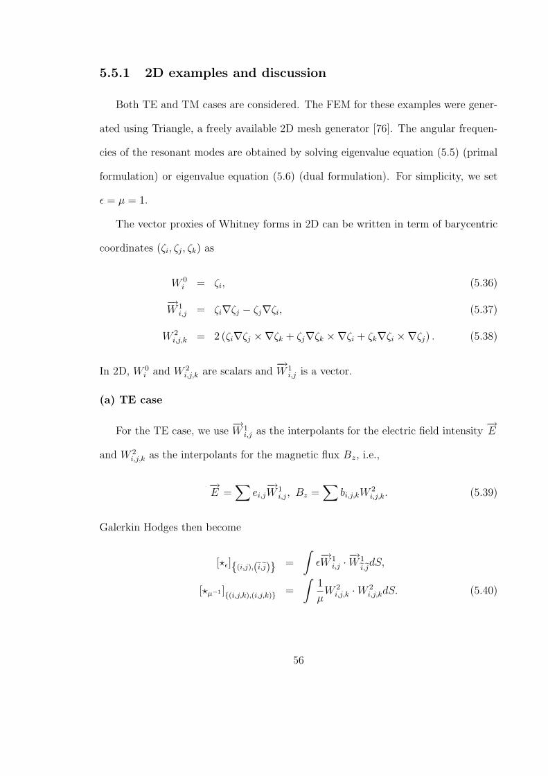
5.5.1 2D examples and discussion

Both TE and TM cases are considered. The FEM for these examples were gener-

ated using Triangle, a freely available 2D mesh generator [76]. The angular frequen-

cies of the resonant modes are obtained by solving eigenvalue equation (5.5) (primal

formulation) or eigenvalue equation (5.6) (dual formulation). For simplicity, we set

ε = µ = 1.

The vector proxies of Whitney forms in 2D can be written in term of barycentric

coordinates (ζi, ζj, ζk) as

W 0i = ζi, (5.36)

−→W 1

i,j = ζi∇ζj − ζj∇ζi, (5.37)

W 2i,j,k = 2 (ζi∇ζj ×∇ζk + ζj∇ζk ×∇ζi + ζk∇ζi ×∇ζj) . (5.38)

In 2D, W 0i and W 2

i,j,k are scalars and−→W 1

i,j is a vector.

(a) TE case

For the TE case, we use−→W 1

i,j as the interpolants for the electric field intensity−→E

and W 2i,j,k as the interpolants for the magnetic flux Bz, i.e.,

−→E =

∑ei,j−→W 1

i,j, Bz =∑

bi,j,kW2i,j,k. (5.39)

Galerkin Hodges then become

[?ε](i,j),(ei,ej) =

∫ε−→W 1

i,j ·−→W 1ei,ejdS,

[?µ−1 ](i,j,k),(i,j,k) =

∫1

µW 2

i,j,k ·W 2i,j,kdS. (5.40)

56

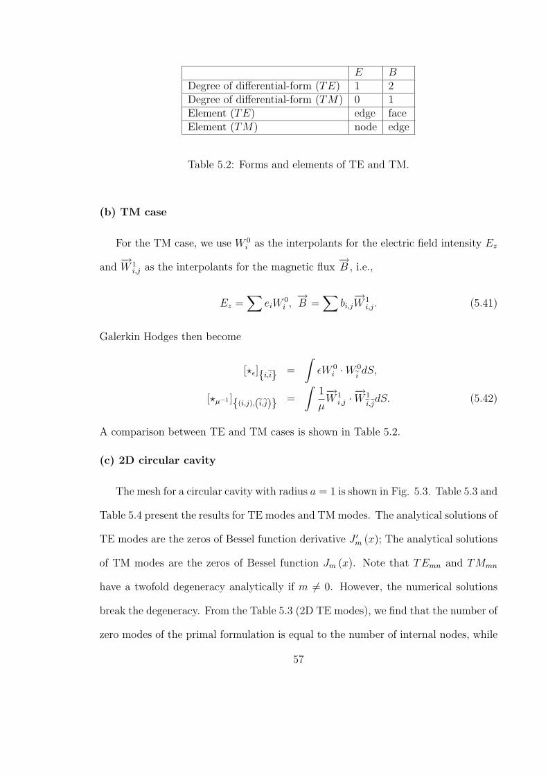
E BDegree of differential-form (TE) 1 2Degree of differential-form (TM) 0 1Element (TE) edge faceElement (TM) node edge

Table 5.2: Forms and elements of TE and TM.

(b) TM case

For the TM case, we use W 0i as the interpolants for the electric field intensity Ez

and−→W 1

i,j as the interpolants for the magnetic flux−→B , i.e.,

Ez =∑

eiW0i ,−→B =

∑bi,j−→W 1

i,j. (5.41)

Galerkin Hodges then become

[?ε]i,ei =

∫εW 0

i ·W 0ei dS,

[?µ−1 ](i,j),(ei,ej) =

∫1

µ

−→W 1

i,j ·−→W 1ei,ejdS. (5.42)

A comparison between TE and TM cases is shown in Table 5.2.

(c) 2D circular cavity

The mesh for a circular cavity with radius a = 1 is shown in Fig. 5.3. Table 5.3 and

Table 5.4 present the results for TE modes and TM modes. The analytical solutions of

TE modes are the zeros of Bessel function derivative J ′m (x); The analytical solutions

of TM modes are the zeros of Bessel function Jm (x). Note that TEmn and TMmn

have a twofold degeneracy analytically if m 6= 0. However, the numerical solutions

break the degeneracy. From the Table 5.3 (2D TE modes), we find that the number of

zero modes of the primal formulation is equal to the number of internal nodes, while

57

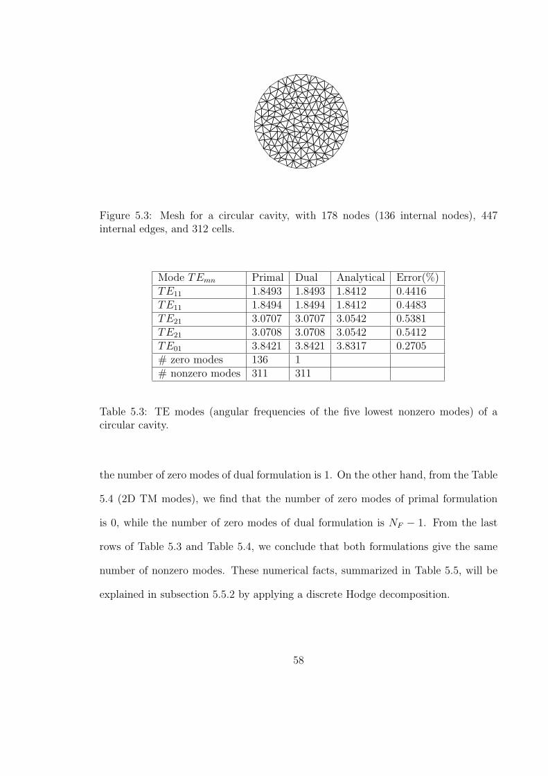
Figure 5.3: Mesh for a circular cavity, with 178 nodes (136 internal nodes), 447internal edges, and 312 cells.

Mode TEmn Primal Dual Analytical Error(%)TE11 1.8493 1.8493 1.8412 0.4416TE11 1.8494 1.8494 1.8412 0.4483TE21 3.0707 3.0707 3.0542 0.5381TE21 3.0708 3.0708 3.0542 0.5412TE01 3.8421 3.8421 3.8317 0.2705# zero modes 136 1# nonzero modes 311 311

Table 5.3: TE modes (angular frequencies of the five lowest nonzero modes) of acircular cavity.

the number of zero modes of dual formulation is 1. On the other hand, from the Table

5.4 (2D TM modes), we find that the number of zero modes of primal formulation

is 0, while the number of zero modes of dual formulation is NF − 1. From the last

rows of Table 5.3 and Table 5.4, we conclude that both formulations give the same

number of nonzero modes. These numerical facts, summarized in Table 5.5, will be

explained in subsection 5.5.2 by applying a discrete Hodge decomposition.

58

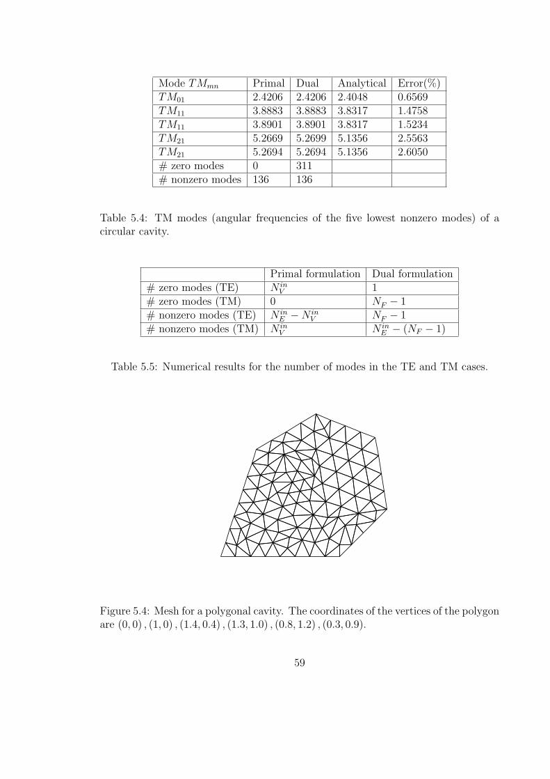
Mode TMmn Primal Dual Analytical Error(%)TM01 2.4206 2.4206 2.4048 0.6569TM11 3.8883 3.8883 3.8317 1.4758TM11 3.8901 3.8901 3.8317 1.5234TM21 5.2669 5.2699 5.1356 2.5563TM21 5.2694 5.2694 5.1356 2.6050# zero modes 0 311# nonzero modes 136 136

Table 5.4: TM modes (angular frequencies of the five lowest nonzero modes) of acircular cavity.

Primal formulation Dual formulation# zero modes (TE) N in

V 1# zero modes (TM) 0 NF − 1# nonzero modes (TE) N in

E −N inV NF − 1

# nonzero modes (TM) N inV N in

E − (NF − 1)

Table 5.5: Numerical results for the number of modes in the TE and TM cases.

Figure 5.4: Mesh for a polygonal cavity. The coordinates of the vertices of the polygonare (0, 0) , (1, 0) , (1.4, 0.4) , (1.3, 1.0) , (0.8, 1.2) , (0.3, 0.9).

59

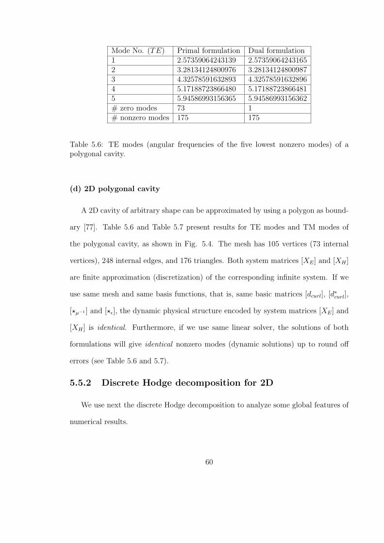
Mode No. (TE) Primal formulation Dual formulation1 2.57359064243139 2.573590642431652 3.28134124800976 3.281341248009873 4.32578591632893 4.325785916328964 5.17188723866480 5.171887238664815 5.94586993156365 5.94586993156362# zero modes 73 1# nonzero modes 175 175

Table 5.6: TE modes (angular frequencies of the five lowest nonzero modes) of apolygonal cavity.

(d) 2D polygonal cavity

A 2D cavity of arbitrary shape can be approximated by using a polygon as bound-

ary [77]. Table 5.6 and Table 5.7 present results for TE modes and TM modes of

the polygonal cavity, as shown in Fig. 5.4. The mesh has 105 vertices (73 internal

vertices), 248 internal edges, and 176 triangles. Both system matrices [XE] and [XH ]

are finite approximation (discretization) of the corresponding infinite system. If we

use same mesh and same basis functions, that is, same basic matrices [dcurl], [d∗curl],

[?µ−1 ] and [?ε], the dynamic physical structure encoded by system matrices [XE] and

[XH ] is identical. Furthermore, if we use same linear solver, the solutions of both

formulations will give identical nonzero modes (dynamic solutions) up to round off

errors (see Table 5.6 and 5.7).

5.5.2 Discrete Hodge decomposition for 2D

We use next the discrete Hodge decomposition to analyze some global features of

numerical results.

60

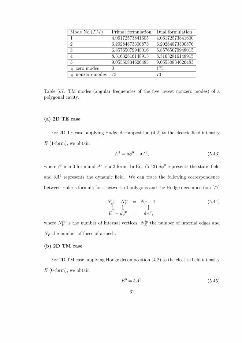
Mode No.(TM) Primal formulation Dual formulation1 4.06172573841605 4.061725738416002 6.20284873300873 6.202848733008763 6.85765079948016 6.857650799480154 8.31632816148913 8.316328161489155 9.05550834626485 9.05550834626483# zero modes 0 175# nonzero modes 73 73

Table 5.7: TM modes (angular frequencies of the five lowest nonzero modes) of apolygonal cavity.

(a) 2D TE case

For 2D TE case, applying Hodge decomposition (4.2) to the electric field intensity

E (1-form), we obtain

E1 = dφ0 + δA2, (5.43)

where φ0 is a 0-form and A2 is a 2-form. In Eq. (5.43) dφ0 represents the static field

and δA2 represents the dynamic field. We can trace the following correspondence

between Euler’s formula for a network of polygons and the Hodge decomposition [77]

N inE −N in

V = NF − 1,l l l

E1 − dφ0 = δA2,

(5.44)

where N inV is the number of internal vertices, N in

E the number of internal edges and

NF the number of faces of a mesh.

(b) 2D TM case

For 2D TM case, applying Hodge decomposition (4.2) to the electric field intensity

E (0-form), we obtain

E0 = δA1, (5.45)

61

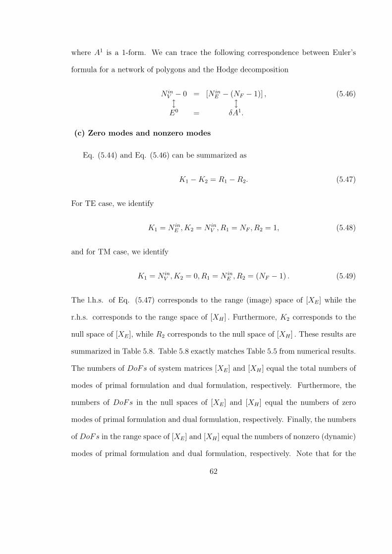
where A1 is a 1-form. We can trace the following correspondence between Euler’s

formula for a network of polygons and the Hodge decomposition

N inV − 0 = [N in

E − (NF − 1)] ,l l

E0 = δA1.

(5.46)

(c) Zero modes and nonzero modes

Eq. (5.44) and Eq. (5.46) can be summarized as

K1 −K2 = R1 −R2. (5.47)

For TE case, we identify

K1 = N inE , K2 = N in

V , R1 = NF , R2 = 1, (5.48)

and for TM case, we identify

K1 = N inV , K2 = 0, R1 = N in

E , R2 = (NF − 1) . (5.49)

The l.h.s. of Eq. (5.47) corresponds to the range (image) space of [XE] while the

r.h.s. corresponds to the range space of [XH ] . Furthermore, K2 corresponds to the

null space of [XE], while R2 corresponds to the null space of [XH ] . These results are

summarized in Table 5.8. Table 5.8 exactly matches Table 5.5 from numerical results.

The numbers of DoFs of system matrices [XE] and [XH ] equal the total numbers of

modes of primal formulation and dual formulation, respectively. Furthermore, the

numbers of DoFs in the null spaces of [XE] and [XH ] equal the numbers of zero

modes of primal formulation and dual formulation, respectively. Finally, the numbers

of DoFs in the range space of [XE] and [XH ] equal the numbers of nonzero (dynamic)

modes of primal formulation and dual formulation, respectively. Note that for the

62

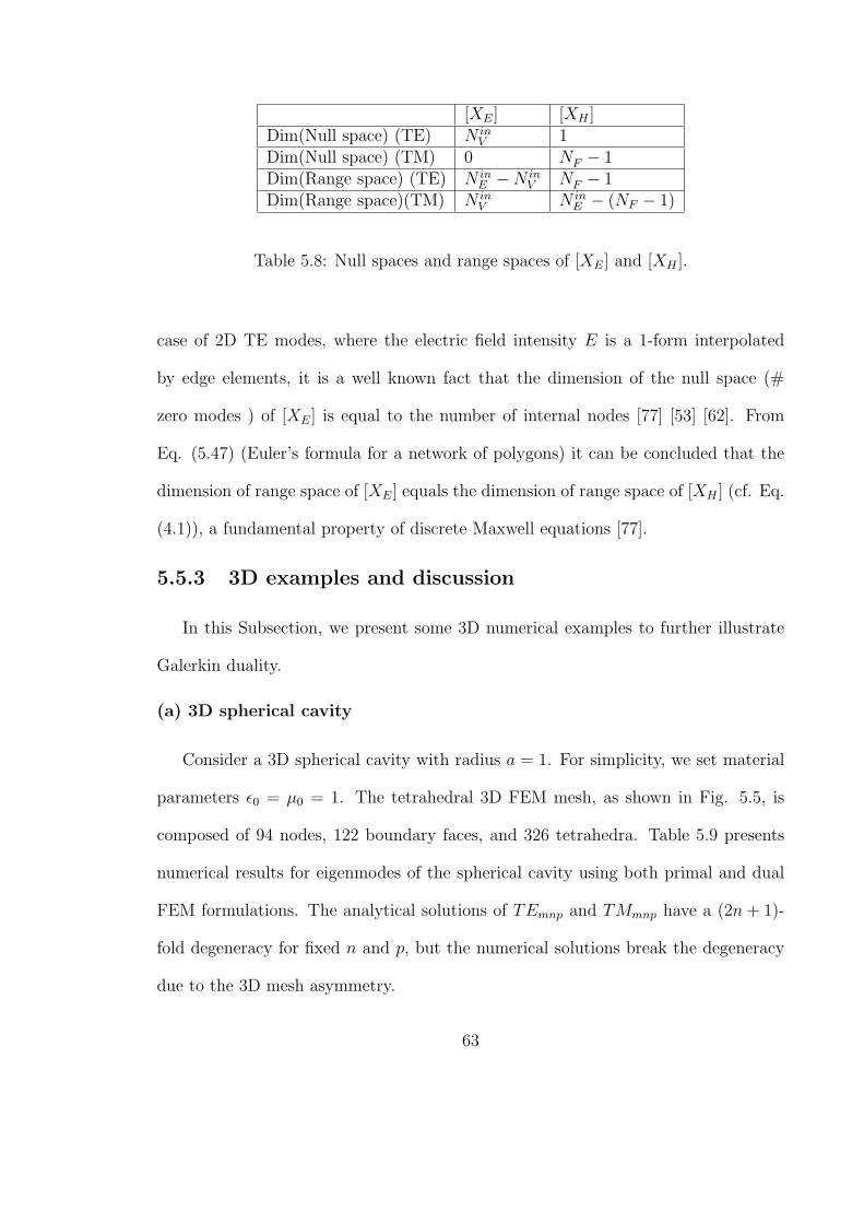
[XE] [XH ]Dim(Null space) (TE) N in

V 1Dim(Null space) (TM) 0 NF − 1Dim(Range space) (TE) N in

E −N inV NF − 1

Dim(Range space)(TM) N inV N in

E − (NF − 1)

Table 5.8: Null spaces and range spaces of [XE] and [XH ].

case of 2D TE modes, where the electric field intensity E is a 1-form interpolated

by edge elements, it is a well known fact that the dimension of the null space (#

zero modes ) of [XE] is equal to the number of internal nodes [77] [53] [62]. From

Eq. (5.47) (Euler’s formula for a network of polygons) it can be concluded that the

dimension of range space of [XE] equals the dimension of range space of [XH ] (cf. Eq.

(4.1)), a fundamental property of discrete Maxwell equations [77].

5.5.3 3D examples and discussion

In this Subsection, we present some 3D numerical examples to further illustrate

Galerkin duality.

(a) 3D spherical cavity

Consider a 3D spherical cavity with radius a = 1. For simplicity, we set material

parameters ε0 = µ0 = 1. The tetrahedral 3D FEM mesh, as shown in Fig. 5.5, is

composed of 94 nodes, 122 boundary faces, and 326 tetrahedra. Table 5.9 presents

numerical results for eigenmodes of the spherical cavity using both primal and dual

FEM formulations. The analytical solutions of TEmnp and TMmnp have a (2n + 1)-

fold degeneracy for fixed n and p, but the numerical solutions break the degeneracy

due to the 3D mesh asymmetry.

63

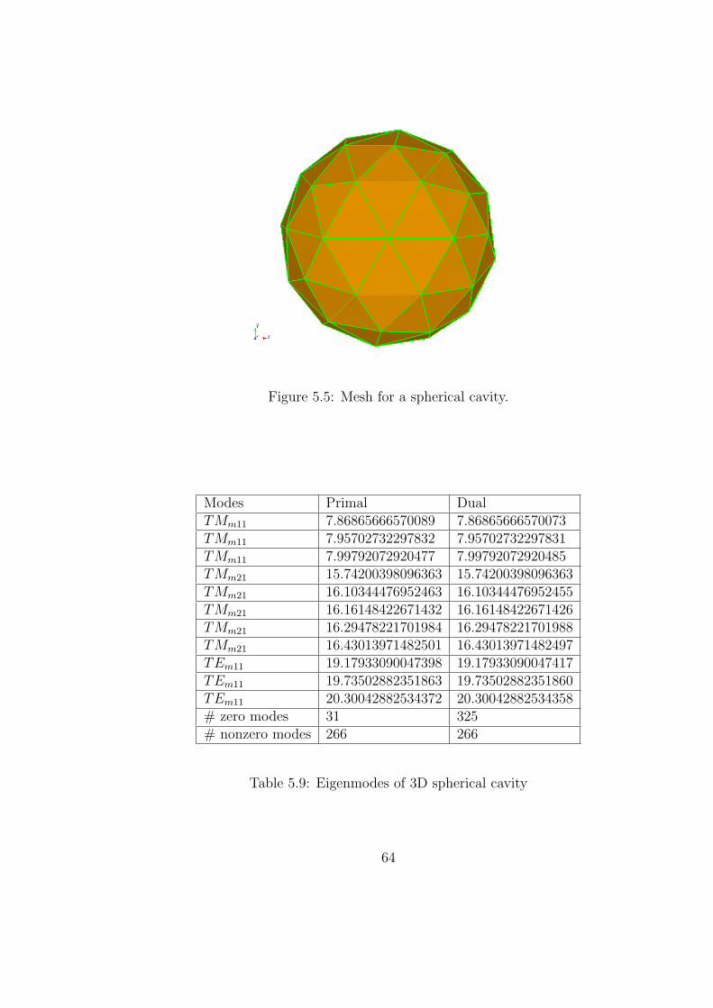
Figure 5.5: Mesh for a spherical cavity.

Modes Primal DualTMm11 7.86865666570089 7.86865666570073TMm11 7.95702732297832 7.95702732297831TMm11 7.99792072920477 7.99792072920485TMm21 15.74200398096363 15.74200398096363TMm21 16.10344476952463 16.10344476952455TMm21 16.16148422671432 16.16148422671426TMm21 16.29478221701984 16.29478221701988TMm21 16.43013971482501 16.43013971482497TEm11 19.17933090047398 19.17933090047417TEm11 19.73502882351863 19.73502882351860TEm11 20.30042882534372 20.30042882534358# zero modes 31 325# nonzero modes 266 266

Table 5.9: Eigenmodes of 3D spherical cavity

64

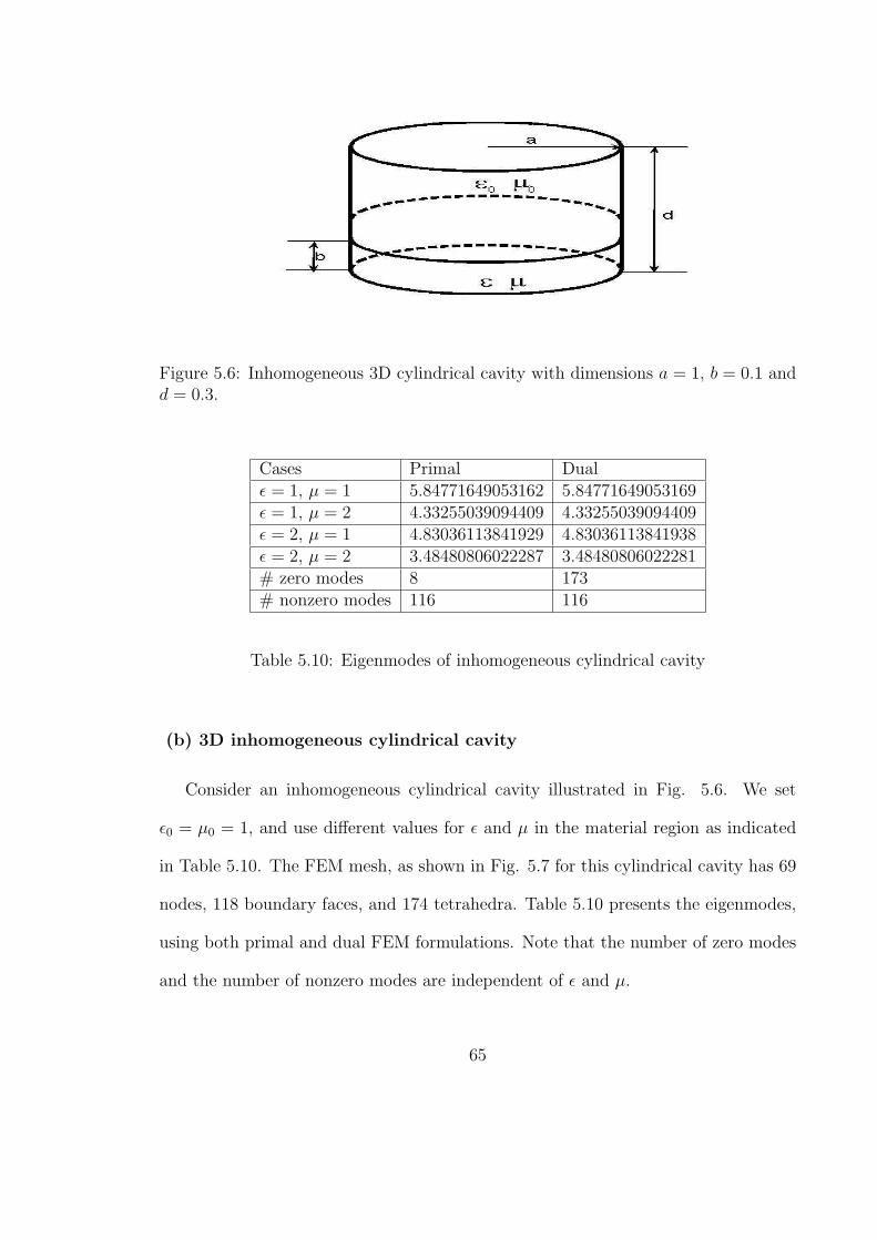
Figure 5.6: Inhomogeneous 3D cylindrical cavity with dimensions a = 1, b = 0.1 andd = 0.3.

Cases Primal Dualε = 1, µ = 1 5.84771649053162 5.84771649053169ε = 1, µ = 2 4.33255039094409 4.33255039094409ε = 2, µ = 1 4.83036113841929 4.83036113841938ε = 2, µ = 2 3.48480806022287 3.48480806022281# zero modes 8 173# nonzero modes 116 116

Table 5.10: Eigenmodes of inhomogeneous cylindrical cavity

(b) 3D inhomogeneous cylindrical cavity

Consider an inhomogeneous cylindrical cavity illustrated in Fig. 5.6. We set

ε0 = µ0 = 1, and use different values for ε and µ in the material region as indicated

in Table 5.10. The FEM mesh, as shown in Fig. 5.7 for this cylindrical cavity has 69

nodes, 118 boundary faces, and 174 tetrahedra. Table 5.10 presents the eigenmodes,

using both primal and dual FEM formulations. Note that the number of zero modes

and the number of nonzero modes are independent of ε and µ.

65

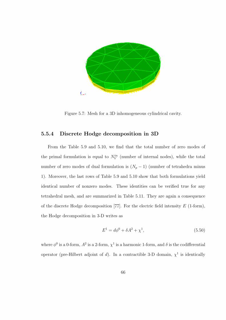
Figure 5.7: Mesh for a 3D inhomogeneous cylindrical cavity.

5.5.4 Discrete Hodge decomposition in 3D

From the Table 5.9 and 5.10, we find that the total number of zero modes of

the primal formulation is equal to N inV (number of internal nodes), while the total

number of zero modes of dual formulation is (Np − 1) (number of tetrahedra minus

1). Moreover, the last rows of Table 5.9 and 5.10 show that both formulations yield

identical number of nonzero modes. These identities can be verified true for any

tetrahedral mesh, and are summarized in Table 5.11. They are again a consequence

of the discrete Hodge decomposition [77]. For the electric field intensity E (1-form),

the Hodge decomposition in 3-D writes as

E1 = dφ0 + δA2 + χ1, (5.50)

where φ0 is a 0-form, A2 is a 2-form, χ1 is a harmonic 1-form, and δ is the codifferential

operator (pre-Hilbert adjoint of d). In a contractible 3-D domain, χ1 is identically

66

Primal formulation Dual formulation# zero modes N in

V Np − 1# nonzero modes N in

E −N inV N in

F − (Np − 1)

Table 5.11: Number of modes from numerical results

[XE] [XH ]dim(Null) N in

V Np − 1dim(Range) N in

E −N inV N in

F − (Np − 1)

Table 5.12: Null space and range space of [XE] and [XH ]

zero. For Maxwell equations, dφ0 in Eq. (5.50) represents the static component of

the electric field and δA2 represents the dynamic component of the electric field.

By considering the FEM mesh as a network of polyhedra, we can trace the fol-

lowing correspondence between Euler’s (polyhedral) formula and the above Hodge

decomposition [77]

N inE −N in

V = [N inF − (Np − 1)] ,

l l lE1 − dφ0 = δA2,

(5.51)

where N inV is the number of internal vertices, N in

E the number of internal edges, N inF

the number of internal faces and Np the number of volumes (tetrahedra) of a mesh.

These results, which are summarized in Table 5.12, exactly match the numerical

results in Table 5.11.

67

CHAPTER 6

SPARSE APPROXIMATION OF INVERSE HODGE(MASS) MATRICES

In the last Chapter, we have discussed primal and dual formulations for the finite

element method (FEM) solutions of the vector wave equations. The primal and dual

formulations yield identical dynamical solutions (up to numerical roundoff). However,

while the primal stiffness matrix [S] and primal mass matrix [M ] are sparse, the dual

stiffness matrix[S†

]and dual mass matrix

[M †] are, in general, not. Fortunately,

it turns out that[S†

]and

[M †] are quasi-sparse because of strong localization prop-

erties of inverse Hodge (mass) matrices. Therefore, we can introduce approaches to

approximate[S†

]and

[M †] by sparse matrices with negligible loss of accuracy. More-

over, based on sparse approximation of inverse Hodge (mass) matrices, a sparse and

explicit (conditionally stable) time domain finite element scheme can be constructed,

as detailed in this Chapter.

68

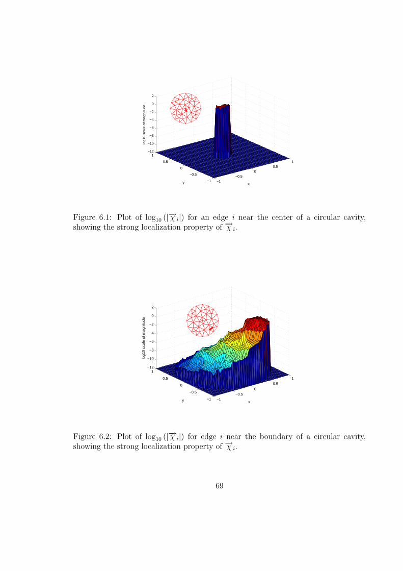
−1−0.5

00.5

1

−1

−0.5

0

0.5

1−12

−10

−8

−6

−4

−2

0

2

xy

log1

0 sc

ale

of m

agni

tude

Figure 6.1: Plot of log10 (|−→χ i|) for an edge i near the center of a circular cavity,showing the strong localization property of −→χ i.

−1−0.5

00.5

1

−1

−0.5

0

0.5

1−12

−10

−8

−6

−4

−2

0

2

xy

log1

0 sc

ale

of m

agni

tude

Figure 6.2: Plot of log10 (|−→χ i|) for edge i near the boundary of a circular cavity,showing the strong localization property of −→χ i.

69

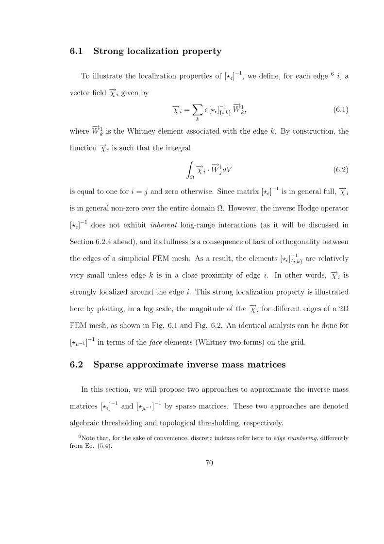
6.1 Strong localization property

To illustrate the localization properties of [?ε]−1, we define, for each edge 6 i, a

vector field −→χ i given by

−→χ i =∑

k

ε [?ε]−1i,k

−→W 1

k, (6.1)

where−→W 1

k is the Whitney element associated with the edge k. By construction, the

function −→χ i is such that the integral

∫

Ω

−→χ i · −→W 1jdV (6.2)

is equal to one for i = j and zero otherwise. Since matrix [?ε]−1 is in general full, −→χ i

is in general non-zero over the entire domain Ω. However, the inverse Hodge operator

[?ε]−1 does not exhibit inherent long-range interactions (as it will be discussed in

Section 6.2.4 ahead), and its fullness is a consequence of lack of orthogonality between

the edges of a simplicial FEM mesh. As a result, the elements [?ε]−1i,k are relatively

very small unless edge k is in a close proximity of edge i. In other words, −→χ i is

strongly localized around the edge i. This strong localization property is illustrated

here by plotting, in a log scale, the magnitude of the −→χ i for different edges of a 2D

FEM mesh, as shown in Fig. 6.1 and Fig. 6.2. An identical analysis can be done for

[?µ−1 ]−1 in terms of the face elements (Whitney two-forms) on the grid.

6.2 Sparse approximate inverse mass matrices

In this section, we will propose two approaches to approximate the inverse mass

matrices [?ε]−1 and [?µ−1 ]−1 by sparse matrices. These two approaches are denoted

algebraic thresholding and topological thresholding, respectively.

6Note that, for the sake of convenience, discrete indexes refer here to edge numbering, differentlyfrom Eq. (5.4).

70

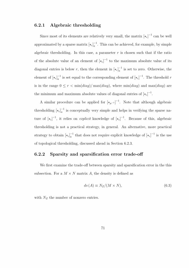
6.2.1 Algebraic thresholding

Since most of its elements are relatively very small, the matrix [?ε]−1 can be well

approximated by a sparse matrix [?ε]−1a . This can be achieved, for example, by simple

algebraic thresholding. In this case, a parameter r is chosen such that if the ratio

of the absolute value of an element of [?ε]−1 to the maximum absolute value of its

diagonal entries is below r, then the element in [?ε]−1a is set to zero. Otherwise, the

element of [?ε]−1a is set equal to the corresponding element of [?ε]

−1. The threshold r

is in the range 0 ≤ r < min(diag)/ max(diag), where min(diag) and max(diag) are

the minimum and maximum absolute values of diagonal entries of [?ε]−1.

A similar procedure can be applied for [?µ−1 ]−1. Note that although algebraic

thresholding [?ε]−1a is conceptually very simple and helps in verifying the sparse na-

ture of [?ε]−1, it relies on explicit knowledge of [?ε]

−1. Because of this, algebraic

thresholding is not a practical strategy, in general. An alternative, more practical

strategy to obtain [?ε]−1a that does not require explicit knowledge of [?ε]

−1 is the use

of topological thresholding, discussed ahead in Section 6.2.3.

6.2.2 Sparsity and sparsification error trade-off

We first examine the trade-off between sparsity and sparsification error in the this

subsection. For a M ×N matrix A, the density is defined as

ds (A) ≡ NZ/(M ×N), (6.3)

with NZ the number of nonzero entries.

71

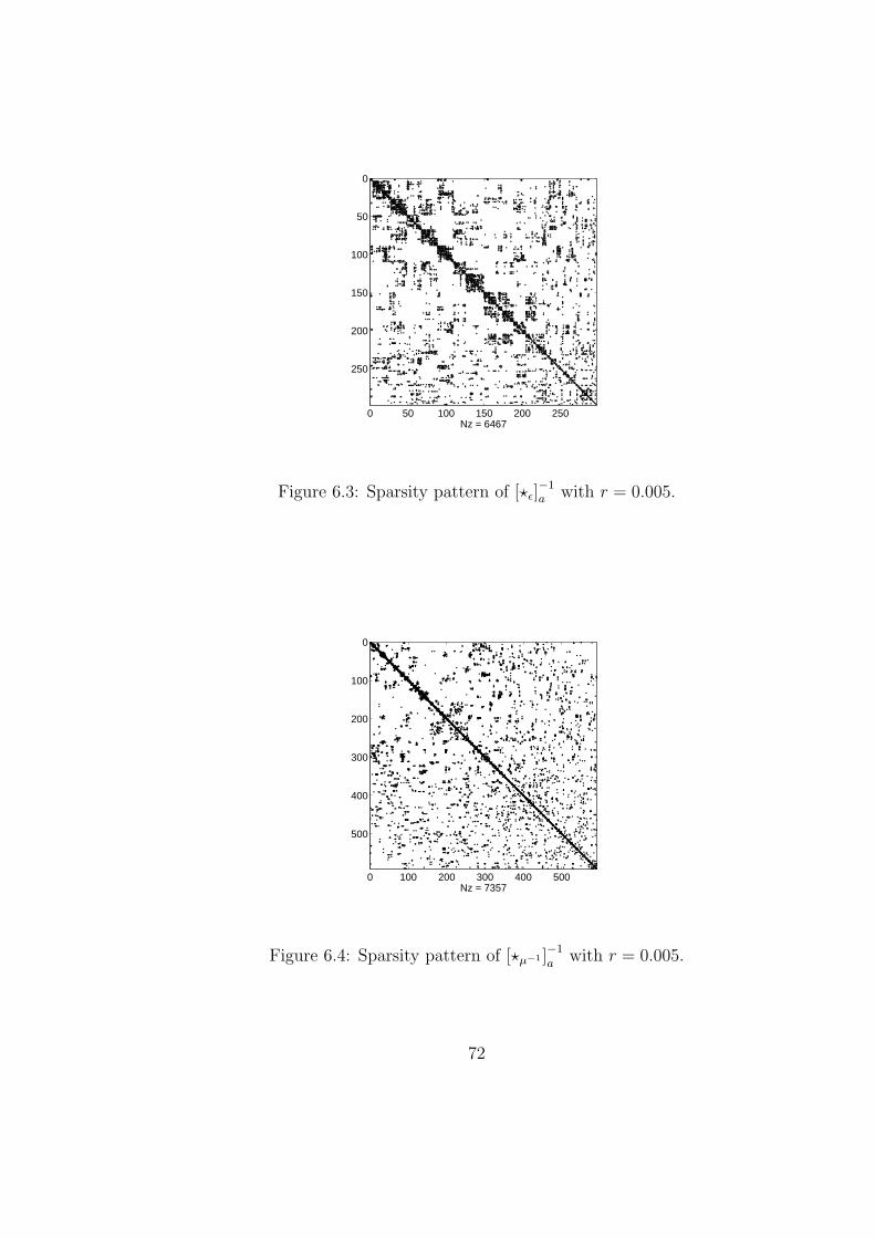
0 50 100 150 200 250

0

50

100

150

200

250

Nz = 6467

Figure 6.3: Sparsity pattern of [?ε]−1a with r = 0.005.

0 100 200 300 400 500

0

100

200

300

400

500

Nz = 7357

Figure 6.4: Sparsity pattern of [?µ−1 ]−1a

with r = 0.005.

72

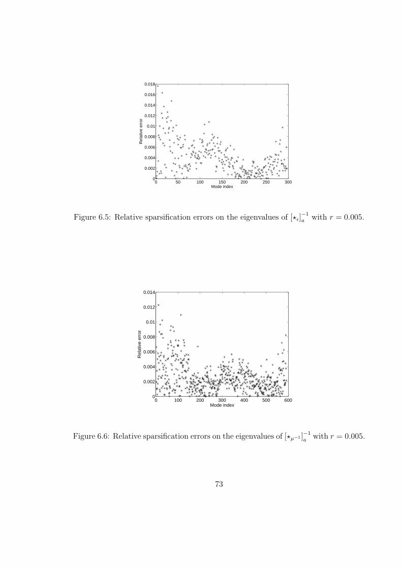
0 50 100 150 200 250 3000

0.002

0.004

0.006

0.008

0.01

0.012

0.014

0.016

0.018

Mode index

Rel

ativ

e er

ror

Figure 6.5: Relative sparsification errors on the eigenvalues of [?ε]−1a with r = 0.005.

0 100 200 300 400 500 6000

0.002

0.004

0.006

0.008

0.01

0.012

0.014

Mode index

Rel

ativ

e er

ror

Figure 6.6: Relative sparsification errors on the eigenvalues of [?µ−1 ]−1a

with r = 0.005.

73

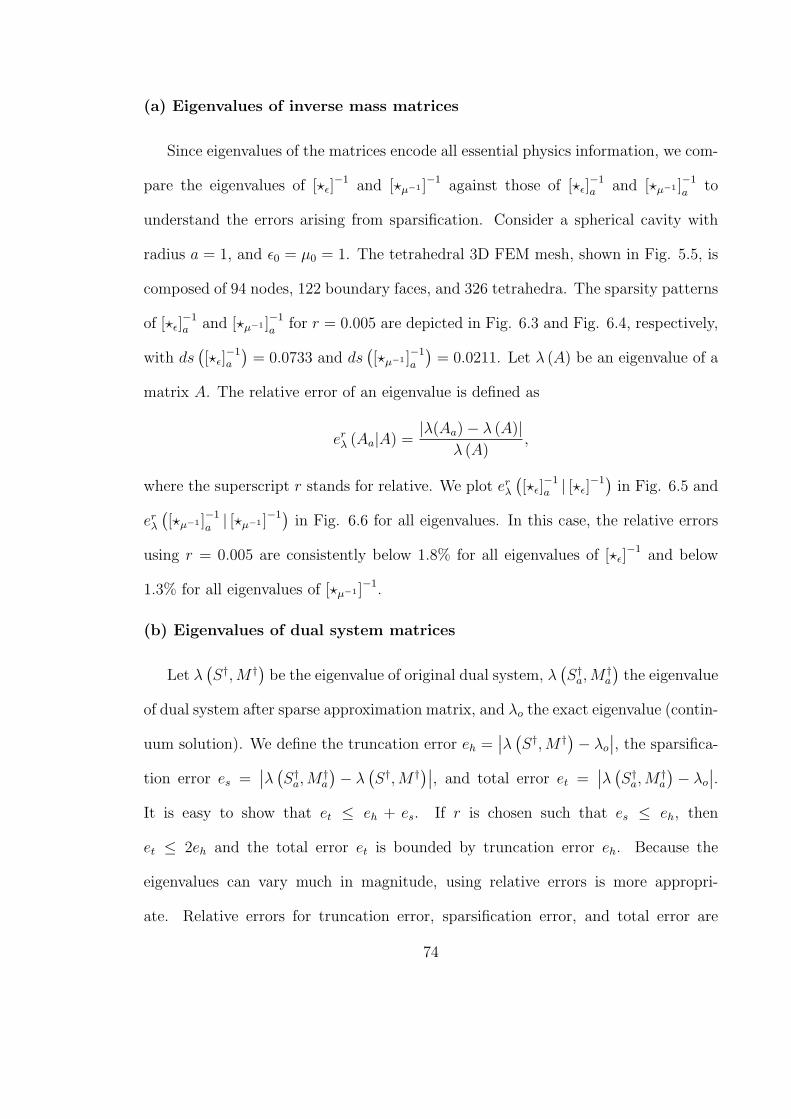
(a) Eigenvalues of inverse mass matrices

Since eigenvalues of the matrices encode all essential physics information, we com-

pare the eigenvalues of [?ε]−1 and [?µ−1 ]−1 against those of [?ε]

−1a and [?µ−1 ]−1

ato

understand the errors arising from sparsification. Consider a spherical cavity with

radius a = 1, and ε0 = µ0 = 1. The tetrahedral 3D FEM mesh, shown in Fig. 5.5, is

composed of 94 nodes, 122 boundary faces, and 326 tetrahedra. The sparsity patterns

of [?ε]−1a and [?µ−1 ]−1

afor r = 0.005 are depicted in Fig. 6.3 and Fig. 6.4, respectively,

with ds([?ε]

−1a

)= 0.0733 and ds

([?µ−1 ]−1

a

)= 0.0211. Let λ (A) be an eigenvalue of a

matrix A. The relative error of an eigenvalue is defined as

erλ (Aa|A) =

|λ(Aa)− λ (A)|λ (A)

,

where the superscript r stands for relative. We plot erλ

([?ε]

−1a | [?ε]

−1) in Fig. 6.5 and

erλ

([?µ−1 ]−1

a| [?µ−1 ]−1) in Fig. 6.6 for all eigenvalues. In this case, the relative errors

using r = 0.005 are consistently below 1.8% for all eigenvalues of [?ε]−1 and below

1.3% for all eigenvalues of [?µ−1 ]−1.

(b) Eigenvalues of dual system matrices

Let λ(S†,M †) be the eigenvalue of original dual system, λ

(S†a,M

†a

)the eigenvalue

of dual system after sparse approximation matrix, and λo the exact eigenvalue (contin-

uum solution). We define the truncation error eh =∣∣λ (

S†,M †)− λo

∣∣, the sparsifica-

tion error es =∣∣λ (

S†a,M†a

)− λ(S†,M †)∣∣, and total error et =

∣∣λ (S†a,M

†a

)− λo

∣∣.

It is easy to show that et ≤ eh + es. If r is chosen such that es ≤ eh, then

et ≤ 2eh and the total error et is bounded by truncation error eh. Because the

eigenvalues can vary much in magnitude, using relative errors is more appropri-

ate. Relative errors for truncation error, sparsification error, and total error are

74

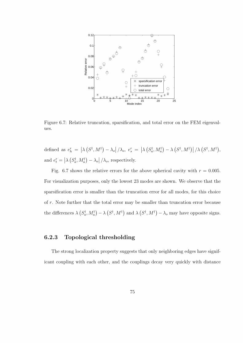
0 5 10 15 20 250

0.02

0.04

0.06

0.08

0.1

0.12

Mode index

Rel

ativ

e er

ror

sparsification error

truncation error

total error

Figure 6.7: Relative truncation, sparsification, and total error on the FEM eigenval-ues.

defined as erh =

∣∣λ (S†,M †)− λo

∣∣ /λo, ers =

∣∣λ (S†a,M

†a

)− λ(S†,M †)∣∣ /λ

(S†,M †),

and ert =

∣∣λ (S†a,M

†a

)− λo

∣∣ /λo, respectively.

Fig. 6.7 shows the relative errors for the above spherical cavity with r = 0.005.

For visualization purposes, only the lowest 23 modes are shown. We observe that the

sparsification error is smaller than the truncation error for all modes, for this choice

of r. Note further that the total error may be smaller than truncation error because

the differences λ(S†a, M

†a

)−λ(S†,M †) and λ

(S†,M †)−λo may have opposite signs.

6.2.3 Topological thresholding

The strong localization property suggests that only neighboring edges have signif-

icant coupling with each other, and the couplings decay very quickly with distance

75

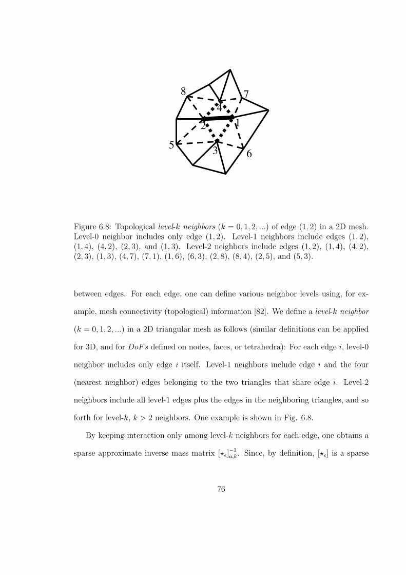
12

5

4

3

7

6

8

Figure 6.8: Topological level-k neighbors (k = 0, 1, 2, ...) of edge (1, 2) in a 2D mesh.Level-0 neighbor includes only edge (1, 2). Level-1 neighbors include edges (1, 2),(1, 4), (4, 2), (2, 3), and (1, 3). Level-2 neighbors include edges (1, 2), (1, 4), (4, 2),(2, 3), (1, 3), (4, 7), (7, 1), (1, 6), (6, 3), (2, 8), (8, 4), (2, 5), and (5, 3).

between edges. For each edge, one can define various neighbor levels using, for ex-

ample, mesh connectivity (topological) information [82]. We define a level-k neighbor

(k = 0, 1, 2, ...) in a 2D triangular mesh as follows (similar definitions can be applied

for 3D, and for DoFs defined on nodes, faces, or tetrahedra): For each edge i, level-0

neighbor includes only edge i itself. Level-1 neighbors include edge i and the four

(nearest neighbor) edges belonging to the two triangles that share edge i. Level-2

neighbors include all level-1 edges plus the edges in the neighboring triangles, and so

forth for level-k, k > 2 neighbors. One example is shown in Fig. 6.8.

By keeping interaction only among level-k neighbors for each edge, one obtains a

sparse approximate inverse mass matrix [?ε]−1a,k. Since, by definition, [?ε] is a sparse

76

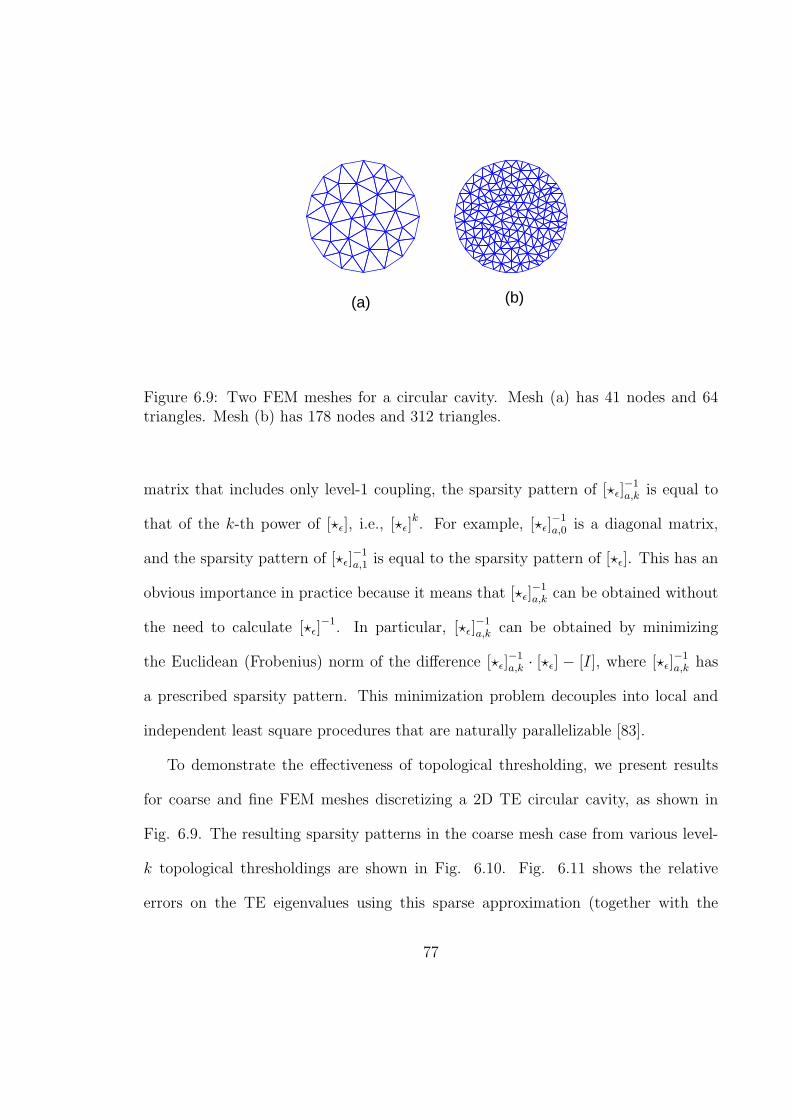
(a) (b)

Figure 6.9: Two FEM meshes for a circular cavity. Mesh (a) has 41 nodes and 64triangles. Mesh (b) has 178 nodes and 312 triangles.

matrix that includes only level-1 coupling, the sparsity pattern of [?ε]−1a,k is equal to

that of the k-th power of [?ε], i.e., [?ε]k. For example, [?ε]

−1a,0 is a diagonal matrix,

and the sparsity pattern of [?ε]−1a,1 is equal to the sparsity pattern of [?ε]. This has an

obvious importance in practice because it means that [?ε]−1a,k can be obtained without

the need to calculate [?ε]−1. In particular, [?ε]

−1a,k can be obtained by minimizing

the Euclidean (Frobenius) norm of the difference [?ε]−1a,k · [?ε] − [I], where [?ε]

−1a,k has

a prescribed sparsity pattern. This minimization problem decouples into local and

independent least square procedures that are naturally parallelizable [83].

To demonstrate the effectiveness of topological thresholding, we present results

for coarse and fine FEM meshes discretizing a 2D TE circular cavity, as shown in

Fig. 6.9. The resulting sparsity patterns in the coarse mesh case from various level-

k topological thresholdings are shown in Fig. 6.10. Fig. 6.11 shows the relative

errors on the TE eigenvalues using this sparse approximation (together with the

77

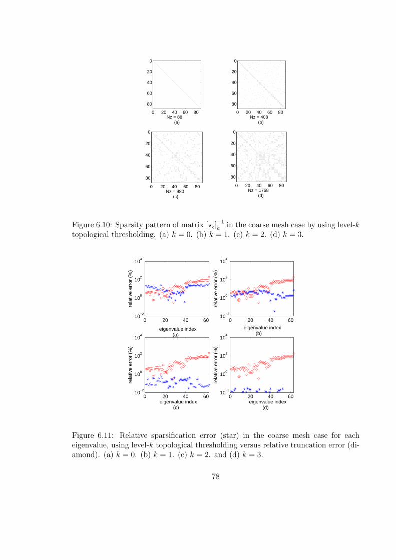
0 20 40 60 80

0

20

40

60

80

Nz = 88 (a)

0 20 40 60 80

0

20

40

60

80

Nz = 408 (b)

0 20 40 60 80

0

20

40

60

80

Nz = 980 (c)

0 20 40 60 80

0

20

40

60

80

Nz = 1768 (d)

Figure 6.10: Sparsity pattern of matrix [?ε]−1a in the coarse mesh case by using level-k

topological thresholding. (a) k = 0. (b) k = 1. (c) k = 2. (d) k = 3.

0 20 40 6010

−2

100

102

104

eigenvalue index (a)

rela

tive

erro

r (%

)

0 20 40 6010

−2

100

102

104

eigenvalue index (b)

rela

tive

erro

r (%

)

0 20 40 6010

−2

100

102

104

eigenvalue index (c)

rela

tive

erro

r (%

)

0 20 40 6010

−2

100

102

104

eigenvalue index (d)

rela

tive

erro

r (%

)

Figure 6.11: Relative sparsification error (star) in the coarse mesh case for eacheigenvalue, using level-k topological thresholding versus relative truncation error (di-amond). (a) k = 0. (b) k = 1. (c) k = 2. and (d) k = 3.

78

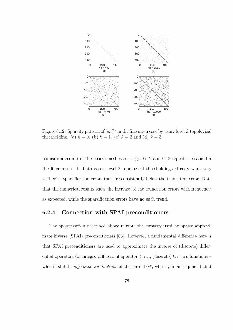
0 200 400

0

100

200

300

400

Nz = 447 (a)

0 200 400

0

100

200

300

400

Nz = 2151 (b)

0 200 400

0

100

200

300

400

Nz = 5403 (c)

0 200 400

0

100

200

300

400

Nz = 10505 (d)

Figure 6.12: Sparsity pattern of [?ε]−1a in the fine mesh case by using level-k topological

thresholding. (a) k = 0. (b) k = 1. (c) k = 2 and (d) k = 3.

truncation errors) in the coarse mesh case. Figs. 6.12 and 6.13 repeat the same for

the finer mesh. In both cases, level-2 topological thresholdings already work very

well, with sparsification errors that are consistently below the truncation error. Note

that the numerical results show the increase of the truncation errors with frequency,

as expected, while the sparsification errors have no such trend.

6.2.4 Connection with SPAI preconditioners

The sparsification described above mirrors the strategy used by sparse approxi-

mate inverse (SPAI) preconditioners [83]. However, a fundamental difference here is

that SPAI preconditioners are used to approximate the inverse of (discrete) differ-

ential operators (or integro-differential operators), i.e., (discrete) Green’s functions –

which exhibit long range interactions of the form 1/rp, where p is an exponent that

79

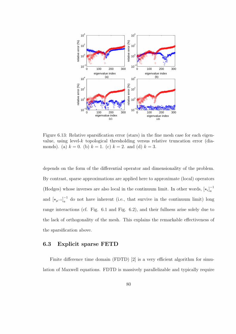
0 100 200 30010

−2

100

102

104

eigenvalue index (a)

rela

tive

erro

r (%

)

0 100 200 30010

−2

100

102

104

eigenvalue index (b)

rela

tive

erro

r (%

)

0 100 200 30010

−2

100

102

104

eigenvalue index (c)

rela

tive

erro

r (%

)

0 100 200 30010

−2

100

102

104

eigenvalue index (d)

rela

tive

erro

r (%

)

Figure 6.13: Relative sparsification error (stars) in the fine mesh case for each eigen-value, using level-k topological thresholding versus relative truncation error (dia-monds). (a) k = 0. (b) k = 1. (c) k = 2. and (d) k = 3.

depends on the form of the differential operator and dimensionality of the problem.

By contrast, sparse approximations are applied here to approximate (local) operators

(Hodges) whose inverses are also local in the continuum limit. In other words, [?ε]−1a

and [?µ−1 ]−1a

do not have inherent (i.e., that survive in the continuum limit) long

range interactions (cf. Fig. 6.1 and Fig. 6.2), and their fullness arise solely due to

the lack of orthogonality of the mesh. This explains the remarkable effectiveness of

the sparsification above.

6.3 Explicit sparse FETD

Finite difference time domain (FDTD) [2] is a very efficient algorithm for simu-

lation of Maxwell equations. FDTD is massively parallelizable and typically require

80

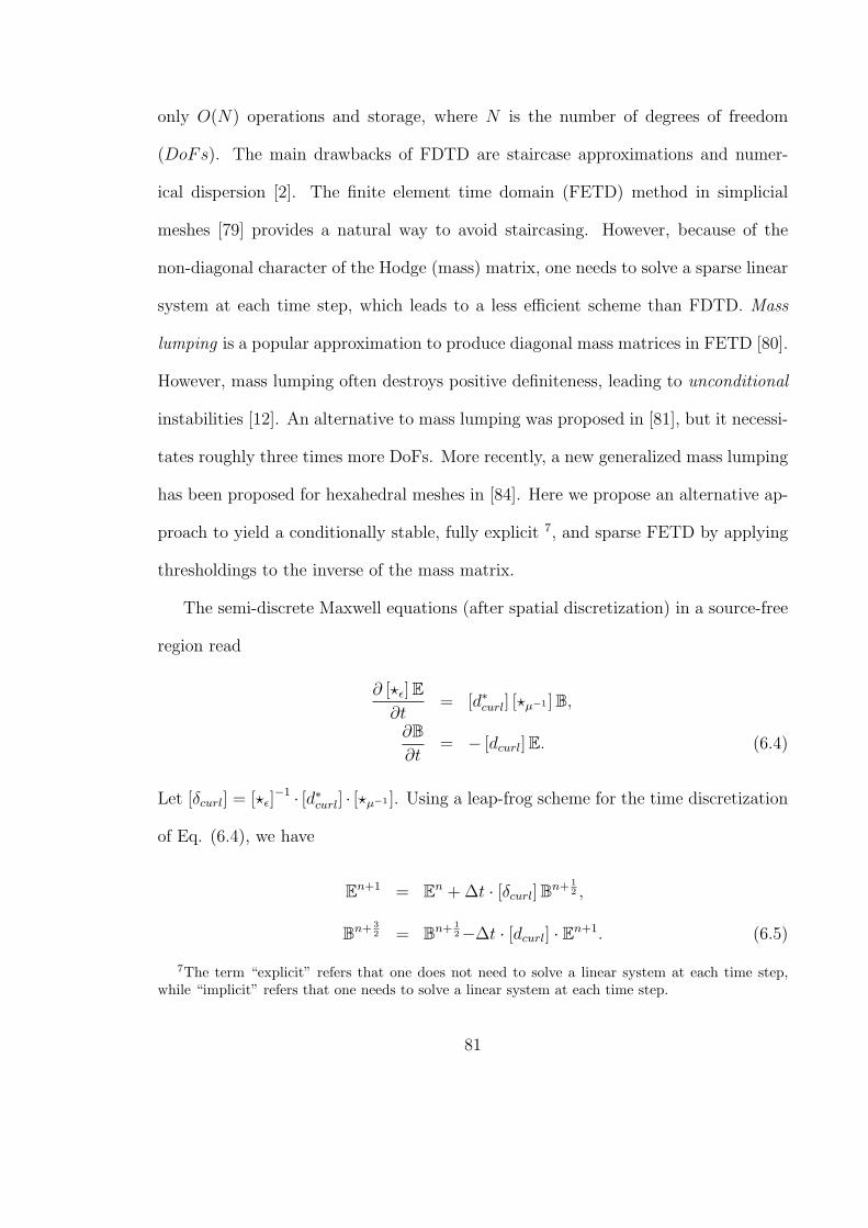
only O(N) operations and storage, where N is the number of degrees of freedom

(DoFs). The main drawbacks of FDTD are staircase approximations and numer-

ical dispersion [2]. The finite element time domain (FETD) method in simplicial

meshes [79] provides a natural way to avoid staircasing. However, because of the

non-diagonal character of the Hodge (mass) matrix, one needs to solve a sparse linear

system at each time step, which leads to a less efficient scheme than FDTD. Mass

lumping is a popular approximation to produce diagonal mass matrices in FETD [80].

However, mass lumping often destroys positive definiteness, leading to unconditional

instabilities [12]. An alternative to mass lumping was proposed in [81], but it necessi-

tates roughly three times more DoFs. More recently, a new generalized mass lumping

has been proposed for hexahedral meshes in [84]. Here we propose an alternative ap-

proach to yield a conditionally stable, fully explicit 7, and sparse FETD by applying

thresholdings to the inverse of the mass matrix.

The semi-discrete Maxwell equations (after spatial discretization) in a source-free

region read

∂ [?ε]E∂t

= [d∗curl] [?µ−1 ]B,

∂B∂t

= − [dcurl]E. (6.4)

Let [δcurl] = [?ε]−1 · [d∗curl] · [?µ−1 ]. Using a leap-frog scheme for the time discretization

of Eq. (6.4), we have

En+1 = En + ∆t · [δcurl]Bn+ 12 ,

Bn+ 32 = Bn+ 1

2−∆t · [dcurl] · En+1. (6.5)

7The term “explicit” refers that one does not need to solve a linear system at each time step,while “implicit” refers that one needs to solve a linear system at each time step.

81

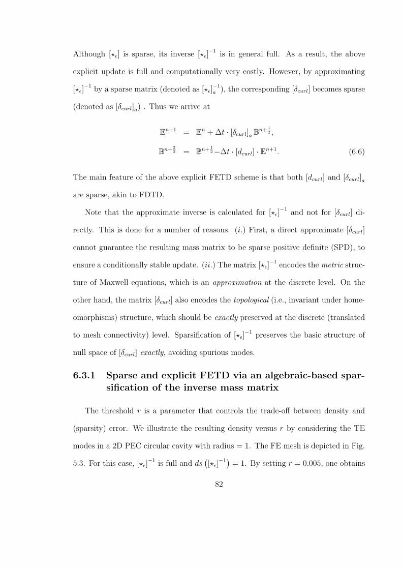
Although [?ε] is sparse, its inverse [?ε]−1 is in general full. As a result, the above

explicit update is full and computationally very costly. However, by approximating

[?ε]−1 by a sparse matrix (denoted as [?ε]

−1a ), the corresponding [δcurl] becomes sparse

(denoted as [δcurl]a) . Thus we arrive at

En+1 = En + ∆t · [δcurl]a Bn+ 1

2 ,

Bn+ 32 = Bn+ 1

2−∆t · [dcurl] · En+1. (6.6)

The main feature of the above explicit FETD scheme is that both [dcurl] and [δcurl]a

are sparse, akin to FDTD.

Note that the approximate inverse is calculated for [?ε]−1 and not for [δcurl] di-

rectly. This is done for a number of reasons. (i.) First, a direct approximate [δcurl]

cannot guarantee the resulting mass matrix to be sparse positive definite (SPD), to

ensure a conditionally stable update. (ii.) The matrix [?ε]−1 encodes the metric struc-

ture of Maxwell equations, which is an approximation at the discrete level. On the

other hand, the matrix [δcurl] also encodes the topological (i.e., invariant under home-

omorphisms) structure, which should be exactly preserved at the discrete (translated

to mesh connectivity) level. Sparsification of [?ε]−1 preserves the basic structure of

null space of [δcurl] exactly, avoiding spurious modes.

6.3.1 Sparse and explicit FETD via an algebraic-based spar-sification of the inverse mass matrix

The threshold r is a parameter that controls the trade-off between density and

(sparsity) error. We illustrate the resulting density versus r by considering the TE

modes in a 2D PEC circular cavity with radius = 1. The FE mesh is depicted in Fig.

5.3. For this case, [?ε]−1 is full and ds

([?ε]

−1) = 1. By setting r = 0.005, one obtains

82

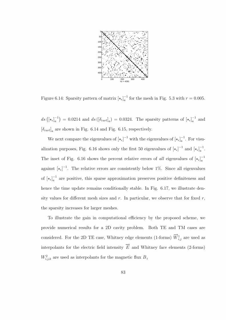
0 100 200 300 400

0

50

100

150

200

250

300

350

400

nz = 4281

Figure 6.14: Sparsity pattern of matrix [?ε]−1a for the mesh in Fig. 5.3 with r = 0.005.

ds([?ε]

−1a

)= 0.0214 and ds ([δcurl]a) = 0.0324. The sparsity patterns of [?ε]

−1a and

[δcurl]a are shown in Fig. 6.14 and Fig. 6.15, respectively.

We next compare the eigenvalues of [?ε]−1 with the eigenvalues of [?ε]

−1a . For visu-

alization purposes, Fig. 6.16 shows only the first 50 eigenvalues of [?ε]−1 and [?ε]

−1a .

The inset of Fig. 6.16 shows the percent relative errors of all eigenvalues of [?ε]−1a

against [?ε]−1. The relative errors are consistently below 1%. Since all eigenvalues

of [?ε]−1a are positive, this sparse approximation preserves positive definiteness and

hence the time update remains conditionally stable. In Fig. 6.17, we illustrate den-

sity values for different mesh sizes and r. In particular, we observe that for fixed r,

the sparsity increases for larger meshes.

To illustrate the gain in computational efficiency by the proposed scheme, we

provide numerical results for a 2D cavity problem. Both TE and TM cases are

considered. For the 2D TE case, Whitney edge elements (1-forms)−→W 1

i,j are used as

interpolants for the electric field intensity−→E and Whitney face elements (2-forms)

W 2i,j,k are used as interpolants for the magnetic flux Bz

83

0 100 200 300

0

50

100

150

200

250

300

350

400

Nz = 4527

Figure 6.15: Sparsity pattern of matrix [δcurl]a for the mesh in Fig. 5.3 with r = 0.005.

0 5 10 15 20 25 30 35 40 45 500.8

0.85

0.9

0.95

1

1.05

1.1

1.15

1.2

1.25

indexes of eigenvalues

eige

nval

ues

0 200 4000

0.20.40.60.8

11.2

indexes of eigenvalues

rela

tive

erro

rs (

%)

inverse of mass matrixinverse of mass matrixby sparse approximations

Figure 6.16: Eigenvalues of mass matrix [?ε]−1 (circle), and eigenvalues of [?ε]

−1a (plus

sign). The inset shows the relative errors (in percent) of eigenvalues of [?ε]−1a against

the eigenvalues of [?ε]−1.

84

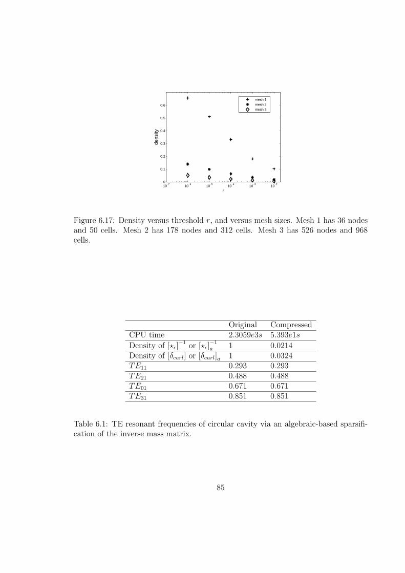
10−7

10−6

10−5

10−4

10−3

10−2

0

0.1

0.2

0.3

0.4

0.5

0.6

r

dens

ity

mesh 1mesh 2mesh 3

Figure 6.17: Density versus threshold r, and versus mesh sizes. Mesh 1 has 36 nodesand 50 cells. Mesh 2 has 178 nodes and 312 cells. Mesh 3 has 526 nodes and 968cells.

Original CompressedCPU time 2.3059e3s 5.393e1s

Density of [?ε]−1 or [?ε]

−1a 1 0.0214

Density of [δcurl] or [δcurl]a 1 0.0324TE11 0.293 0.293TE21 0.488 0.488TE01 0.671 0.671TE31 0.851 0.851

Table 6.1: TE resonant frequencies of circular cavity via an algebraic-based sparsifi-cation of the inverse mass matrix.

85

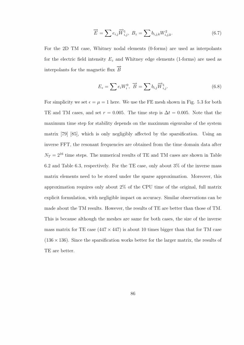
−→E =

∑ei,j−→W 1

i,j, Bz =∑

bi,j,kW2i,j,k. (6.7)

For the 2D TM case, Whitney nodal elements (0-forms) are used as interpolants

for the electric field intensity Ez and Whitney edge elements (1-forms) are used as

interpolants for the magnetic flux−→B

Ez =∑

eiW0i ,−→B =

∑bi,j−→W 1

i,j. (6.8)

For simplicity we set ε = µ = 1 here. We use the FE mesh shown in Fig. 5.3 for both

TE and TM cases, and set r = 0.005. The time step is ∆t = 0.005. Note that the

maximum time step for stability depends on the maximum eigenvalue of the system

matrix [79] [85], which is only negligibly affected by the sparsification. Using an

inverse FFT, the resonant frequencies are obtained from the time domain data after

NT = 216 time steps. The numerical results of TE and TM cases are shown in Table

6.2 and Table 6.3, respectively. For the TE case, only about 3% of the inverse mass

matrix elements need to be stored under the sparse approximation. Moreover, this

approximation requires only about 2% of the CPU time of the original, full matrix

explicit formulation, with negligible impact on accuracy. Similar observations can be

made about the TM results. However, the results of TE are better than those of TM.

This is because although the meshes are same for both cases, the size of the inverse

mass matrix for TE case (447× 447) is about 10 times bigger than that for TM case

(136× 136). Since the sparsification works better for the larger matrix, the results of

TE are better.

86

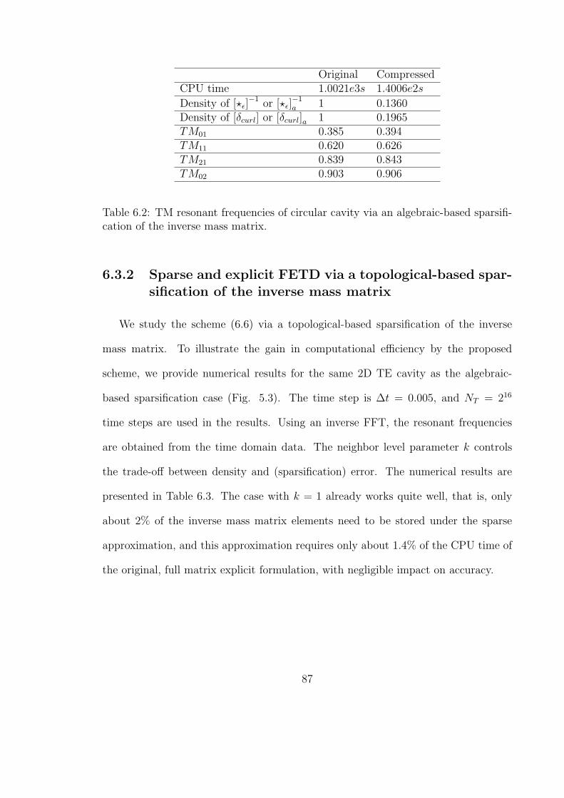
Original CompressedCPU time 1.0021e3s 1.4006e2s


−1a 1 0.1360

Density of [δcurl] or [δcurl]a 1 0.1965TM01 0.385 0.394TM11 0.620 0.626TM21 0.839 0.843TM02 0.903 0.906

Table 6.2: TM resonant frequencies of circular cavity via an algebraic-based sparsifi-cation of the inverse mass matrix.

6.3.2 Sparse and explicit FETD via a topological-based spar-sification of the inverse mass matrix

We study the scheme (6.6) via a topological-based sparsification of the inverse

mass matrix. To illustrate the gain in computational efficiency by the proposed

scheme, we provide numerical results for the same 2D TE cavity as the algebraic-

based sparsification case (Fig. 5.3). The time step is ∆t = 0.005, and NT = 216

time steps are used in the results. Using an inverse FFT, the resonant frequencies

are obtained from the time domain data. The neighbor level parameter k controls

the trade-off between density and (sparsification) error. The numerical results are

presented in Table 6.3. The case with k = 1 already works quite well, that is, only

about 2% of the inverse mass matrix elements need to be stored under the sparse

approximation, and this approximation requires only about 1.4% of the CPU time of

the original, full matrix explicit formulation, with negligible impact on accuracy.

87

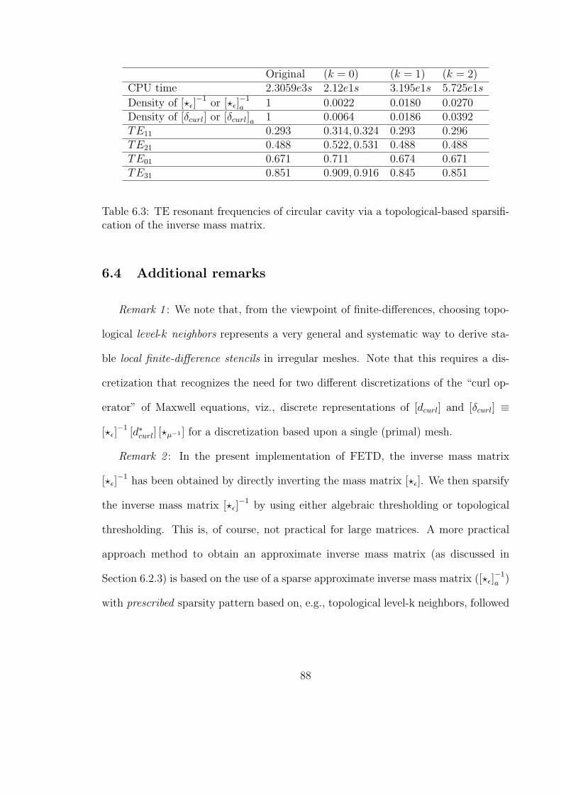
Original (k = 0) (k = 1) (k = 2)CPU time 2.3059e3s 2.12e1s 3.195e1s 5.725e1s


−1a 1 0.0022 0.0180 0.0270

Density of [δcurl] or [δcurl]a 1 0.0064 0.0186 0.0392TE11 0.293 0.314, 0.324 0.293 0.296TE21 0.488 0.522, 0.531 0.488 0.488TE01 0.671 0.711 0.674 0.671TE31 0.851 0.909, 0.916 0.845 0.851

Table 6.3: TE resonant frequencies of circular cavity via a topological-based sparsifi-cation of the inverse mass matrix.


Remark 1 : We note that, from the viewpoint of finite-differences, choosing topo-

logical level-k neighbors represents a very general and systematic way to derive sta-

ble local finite-difference stencils in irregular meshes. Note that this requires a dis-

cretization that recognizes the need for two different discretizations of the “curl op-

erator” of Maxwell equations, viz., discrete representations of [dcurl] and [δcurl] ≡

[?ε]−1 [d∗curl] [?µ−1 ] for a discretization based upon a single (primal) mesh.

Remark 2 : In the present implementation of FETD, the inverse mass matrix

[?ε]−1 has been obtained by directly inverting the mass matrix [?ε]. We then sparsify

the inverse mass matrix [?ε]−1 by using either algebraic thresholding or topological

thresholding. This is, of course, not practical for large matrices. A more practical

approach method to obtain an approximate inverse mass matrix (as discussed in

Section 6.2.3) is based on the use of a sparse approximate inverse mass matrix ([?ε]−1a )

with prescribed sparsity pattern based on, e.g., topological level-k neighbors, followed

88

by the minimization of the Euclidean (Frobenius) norm of the difference ([?ε]−1a · [?ε]−

[I]).

89

CHAPTER 7

AN E-B MIXED FINITE ELEMENT METHOD

The mixed finite element method (FEM) has been successfully developed and

applied to structural mechanics, fluid mechanics, and recently, electromagnetics [86]

[87] [88]. For electromagnetics, mixed FEM has been mostly applied to magnetostatic,

electrostatic [88] [89] [90], and eddy current problems [91]. In a mixed FEM, one uses

two (or more) state variables [86] [87] [88]. Based on the use of the electric field

intensity−→E and magnetic field intensity

−→H as the state variables, mixed FEMs have

been proposed for time-dependent Maxwell’s equations in [92] [93].

We propose here a mixed FEM based on use the electric field intensity−→E and

magnetic field flux−→B (instead of magnetic field intensity

−→H ) as the state variables.

It is natural that one uses edge elements as the interpolants for the electric field

intensity−→E and face elements as the interpolants for the magnetic flux

−→B . This can

guarantee tangential continuity of−→E and normal continuity of

−→B . Furthermore, this

discretization of−→E and

−→B automatically conforms to a discrete version de Rham

diagram in an exact fashion [94] [53], a necessary condition to avoid problems such as

spurious modes, as discussed in previous Chapters. Also of importance is that such

mixed FEM results in sparse matrices, in contrast to the previously proposed E-H

approach [93].

90

7.1 Formulation

As discussed in Chapter 3, the discrete Maxwell equations in source-free, three-

dimensional (3D) space (in the Fourier domain) read

[dcurl]E = iωB, [d∗curl]H=−iωD, (7.1)

[ddiv]B = 0, [d∗div]D=0. (7.2)

Discrete constitutive equations can be written as follows

D = [?ε]E, H = [?µ−1 ]B, (7.3)

where the matrices [?ε] and [?µ−1 ] are discrete Hodge operators. In this Chapter, we

use Galerkin’s Hodges based on Whitney edge and face elements on tetrahedron, that

is,

[?ε](i,j),(ei,ej) =

∫

R3

ε−→W 1

i,j ·−→W 1ei,ejdV,

[?µ−1 ](i,j,k),(ei,ej,ek) =

∫

R3

1

µ

−→W 2

i,j,k ·−→W 2ei,ej,ekdV. (7.4)

As discussed in Chapter 2, Whitney spaces W 1 and W 2, which are spanned by

−→W 1

i,j and−→W 2

i,j,k, respectively, observe the following de Rham relation

W 1 ∇×7→ W 2. (7.5)

The above follows the de Rham diagram [48] [53] [6] [5]:

H (curl, Ω)d7→ H (div, Ω) , (7.6)

since Whitney edge elements and face elements form discrete bases for Sobolev spaces

H(curl, Ω) and H(div, Ω), respectively.

91

Plugging Eqs. (7.3) into Eqs. (7.1) and Eqs. (7.2), we have

[dcurl]E = iωB, [d∗curl] [?µ−1 ]B=−iω [?ε]E, (7.7)

[ddiv]B = 0, [d∗div] [?ε]E=0. (7.8)

Let

[A] =

[[dcurl] 0

0 − [d∗curl] [?µ−1 ]

], (7.9)

[B] =

[0 [I]

[?ε] 0

], (7.10)

where [I] is an identity matrix, and λ = iω, and X = [E B], Eqs. (7.7) can be cast

as the generalized eigenvalue problem

[A]X = λ [B]X. (7.11)

Note that both [A] and [B] are sparse matrices.

If 〈λ,X〉 with X = [E B] is a solution of Eq. (7.11), then⟨−λ,X†

⟩with X† =

[E − B] is also a solution of Eq. (7.11).

7.2 Numerical examples

We next consider the solution of (7.11) in a number of canonical geometries. The

eigenvalues λ of the resonant modes are computed by solving the eigenvalue equation

(7.11). In all numerical examples, for simplicity, we set ε0 = µ0 = 1.

7.2.1 2D circular cavity

Table 7.1 and 7.2 present the results for TE modes and TM modes of a circular

cavity with radius a = 1. The mesh, shown in Fig. 5.3, has 178 vertices (136

internal vertices), 447 internal edges and 312 triangles. In table 7.1 and 7.2, we only

92

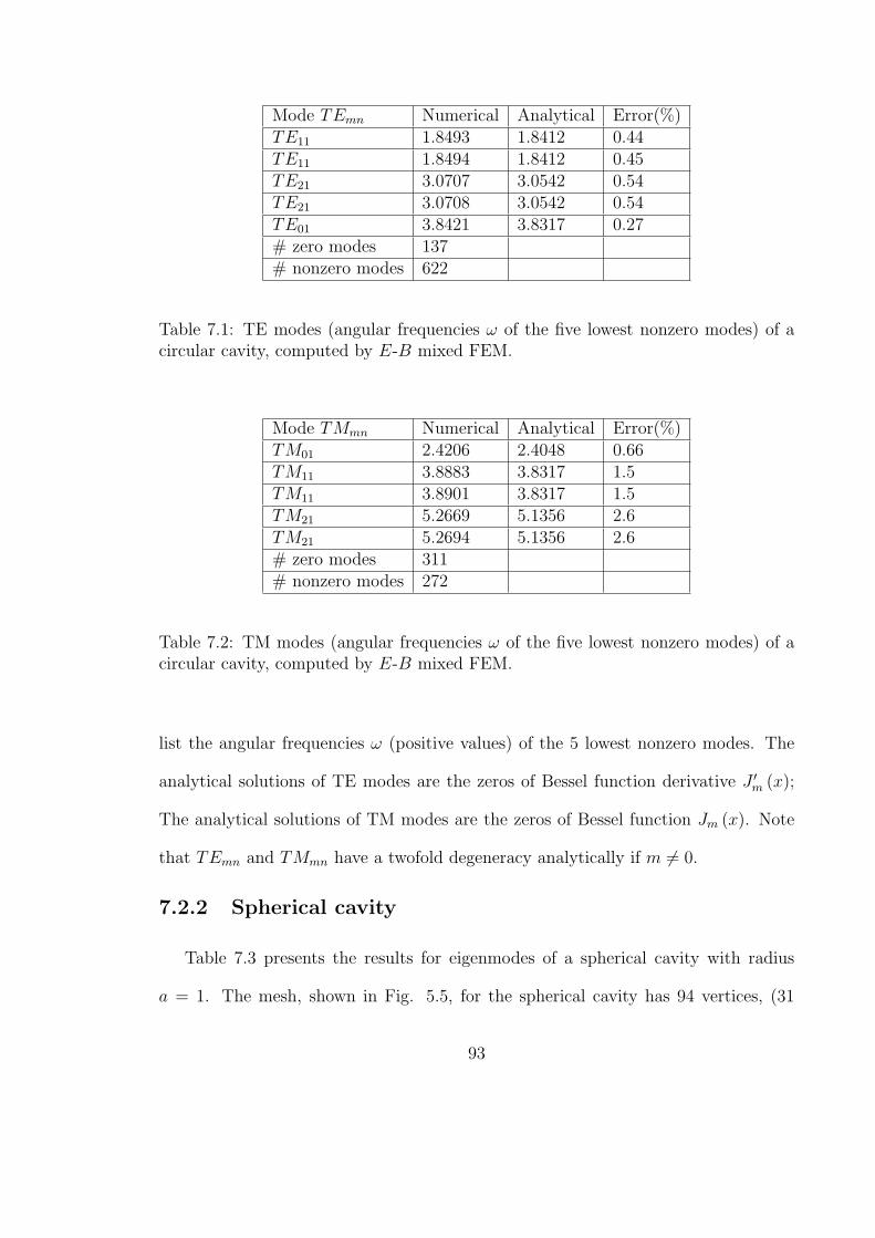
Mode TEmn Numerical Analytical Error(%)TE11 1.8493 1.8412 0.44TE11 1.8494 1.8412 0.45TE21 3.0707 3.0542 0.54TE21 3.0708 3.0542 0.54TE01 3.8421 3.8317 0.27# zero modes 137# nonzero modes 622

Table 7.1: TE modes (angular frequencies ω of the five lowest nonzero modes) of acircular cavity, computed by E-B mixed FEM.

Mode TMmn Numerical Analytical Error(%)TM01 2.4206 2.4048 0.66TM11 3.8883 3.8317 1.5TM11 3.8901 3.8317 1.5TM21 5.2669 5.1356 2.6TM21 5.2694 5.1356 2.6# zero modes 311# nonzero modes 272

Table 7.2: TM modes (angular frequencies ω of the five lowest nonzero modes) of acircular cavity, computed by E-B mixed FEM.

list the angular frequencies ω (positive values) of the 5 lowest nonzero modes. The

analytical solutions of TE modes are the zeros of Bessel function derivative J ′m (x);

The analytical solutions of TM modes are the zeros of Bessel function Jm (x). Note

that TEmn and TMmn have a twofold degeneracy analytically if m 6= 0.

7.2.2 Spherical cavity

Table 7.3 presents the results for eigenmodes of a spherical cavity with radius

a = 1. The mesh, shown in Fig. 5.5, for the spherical cavity has 94 vertices, (31

93

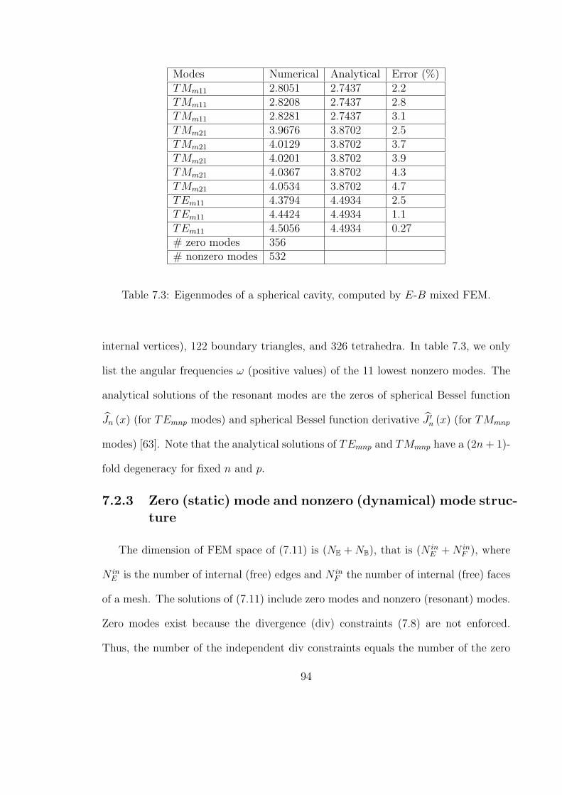
Modes Numerical Analytical Error (%)TMm11 2.8051 2.7437 2.2TMm11 2.8208 2.7437 2.8TMm11 2.8281 2.7437 3.1TMm21 3.9676 3.8702 2.5TMm21 4.0129 3.8702 3.7TMm21 4.0201 3.8702 3.9TMm21 4.0367 3.8702 4.3TMm21 4.0534 3.8702 4.7TEm11 4.3794 4.4934 2.5TEm11 4.4424 4.4934 1.1TEm11 4.5056 4.4934 0.27# zero modes 356# nonzero modes 532

Table 7.3: Eigenmodes of a spherical cavity, computed by E-B mixed FEM.

internal vertices), 122 boundary triangles, and 326 tetrahedra. In table 7.3, we only

list the angular frequencies ω (positive values) of the 11 lowest nonzero modes. The

analytical solutions of the resonant modes are the zeros of spherical Bessel function

Jn (x) (for TEmnp modes) and spherical Bessel function derivative J ′n (x) (for TMmnp

modes) [63]. Note that the analytical solutions of TEmnp and TMmnp have a (2n + 1)-

fold degeneracy for fixed n and p.

7.2.3 Zero (static) mode and nonzero (dynamical) mode struc-ture

The dimension of FEM space of (7.11) is (NE + NB), that is (N inE + N in

F ), where

N inE is the number of internal (free) edges and N in

F the number of internal (free) faces

of a mesh. The solutions of (7.11) include zero modes and nonzero (resonant) modes.

Zero modes exist because the divergence (div) constraints (7.8) are not enforced.

Thus, the number of the independent div constraints equals the number of the zero

94

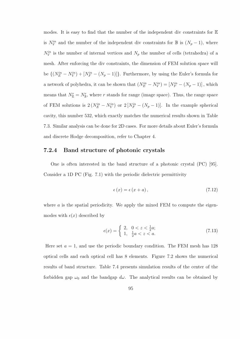
modes. It is easy to find that the number of the independent div constraints for E

is N inV and the number of the independent div constraints for B is (Np − 1), where

N inV is the number of internal vertices and Np the number of cells (tetrahedra) of a

mesh. After enforcing the div constraints, the dimension of FEM solution space will

be (N inE −N in

V ) + [N inF − (Np − 1)]. Furthermore, by using the Euler’s formula for

a network of polyhedra, it can be shown that (N inE −N in

V ) = [N inF − (Np − 1)] , which

means that N rE = N r

B, where r stands for range (image space). Thus, the range space

of FEM solutions is 2 (N inE −N in

V ) or 2 [N inF − (Np − 1)]. In the example spherical

cavity, this number 532, which exactly matches the numerical results shown in Table

7.3. Similar analysis can be done for 2D cases. For more details about Euler’s formula

and discrete Hodge decomposition, refer to Chapter 4.

7.2.4 Band structure of photonic crystals

One is often interested in the band structure of a photonic crystal (PC) [95].

Consider a 1D PC (Fig. 7.1) with the periodic dielectric permittivity

ε (x) = ε (x + a) , (7.12)

where a is the spatial periodicity. We apply the mixed FEM to compute the eigen-

modes with ε(x) described by

ε(x) =

2, 0 < z < 1

2a;

1, 12a < z < a.

(7.13)

Here set a = 1, and use the periodic boundary condition. The FEM mesh has 128

optical cells and each optical cell has 8 elements. Figure 7.2 shows the numerical

results of band structure. Table 7.4 presents simulation results of the center of the

forbidden gap ω0 and the bandgap dω. The analytical results can be obtained by

95

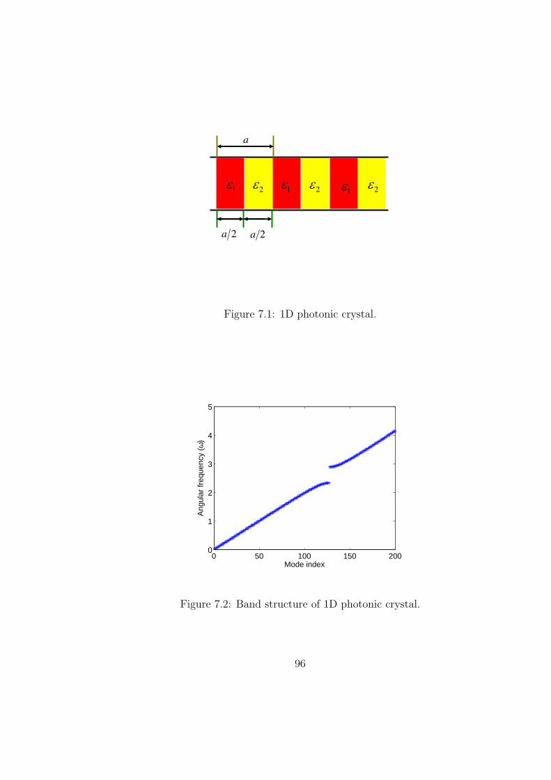
1 2 1 212

a

a 2 a 2

Figure 7.1: 1D photonic crystal.

0 50 100 150 2000

1

2

3

4

5

Mode index

Ang

ular

freq

uenc

y (ω

)

Figure 7.2: Band structure of 1D photonic crystal.

96

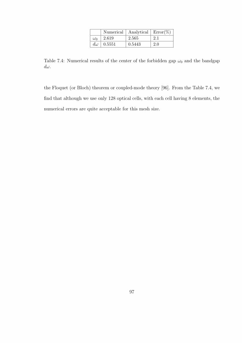
Numerical Analytical Error(%)ω0 2.619 2.565 2.1dω 0.5551 0.5443 2.0

Table 7.4: Numerical results of the center of the forbidden gap ω0 and the bandgapdω.

the Floquet (or Bloch) theorem or coupled-mode theory [96]. From the Table 7.4, we

find that although we use only 128 optical cells, with each cell having 8 elements, the

numerical errors are quite acceptable for this mesh size.

97

CHAPTER 8

GAUGING IN DISCRETE SPACES

Because the electric field intensity E is a differential 1-form that associates with

edges, edge elements should be used for FEM formulation of the wave equations

having the electric field intensity as the unknown. However, stiffness matrices (as well

as system matrices), constructed by edge elements are generally singular matrices due

to the null space of the curl operator. This singularity often causes convergence and/or

low-frequency instabilities problems for FEM solutions in the frequency domain [11].

For FETD based on second order wave equations, this singularity produces spurious

solutions with linear time growth, which can destroy the actual solutions [97] [98]. In

this Chapter, we discuss these problems, and propose some remedies for them.

8.1 Singularity of the curl operator

Consider here an eigenvalue cavity problem with PEC boundary conditions 8, i.e.,

find nonzero−→E : Ω ⊂ R3, and λ ∈ R such that

−→∇ ×−→∇ ×−→E = λ−→E ,

−→∇ · −→E = 0 in Ω,−→E × n on ∂Ω, (8.1)

8Throughout this Chapter, we consider PEC boundary conditions, and set ε and µ equal to one,for simplicity.

98

where ∂Ω is the boundary of Ω. The solution of Eq. (8.1) is well-posed and uniquely

defined. However, if one drops the divergence-free condition (in this dissertation, this

condition is also called gauge condition)

−→∇ · −→E = 0, (8.2)

Problem (8.1) becomes to find a nonzero−→E : Ω ⊂ R3, λ ∈ R such that

−→∇ ×−→∇ ×−→E = λ−→E ,−→E × n on ∂Ω, (8.3)

whose solution is not unique. Namely, suppose that−→E i is a solution of (8.3). Then

−→E i+

−→∇φ is also a solution because

−→∇ ×(−→

E i +−→∇φ

)=−→∇ ×−→E i, (8.4)

where φ is an arbitrary continuous function. If one chooses Whitney 1-forms [27] as

the basis functions for−→E , the above Problem (8.3) with λ 6= 0 is equivalent to Problem

(8.1) [53]. This is because the gauge (divergence-free) condition is satisfied locally

due to the (intra-element) divergence-free property of Whitney 1-forms. However,

Problem (8.3) still admits nontrivial solution with λ = 0, which corresponding to the

null space of curl operator. This null space often causes the low frequency instabilities

[11] and produces spurious solution with linear time growth [97] [98]. It will be

discussed ahead that null space can be removed in the discrete space by enforcing

global divergence-free conditions. Since the essential conclusions here remain valid in

either 2D or 3D, we discuss 2D examples in what follows.

8.2 Constraint equations

As discussed in Section 8.1, finite element solutions (based on edge elements) of

the curl curl equation can be classified into the zero eigenspace and nonzero eigenspace

99

solutions. The zero eigenspace corresponds to static fields that can be described by

scalar potential φ. Let−→E d be the dynamic component, which corresponds to the

nonzero eigenspace. The Hodge (-Helmholtz) decomposition

−→E = −−→∇φ +

−→E d, (8.5)

implies that zero eigenspace is orthogonal to the nonzero eigenspace [103]

∫

Ω

ε−→∇φ · −→E ddΩ = 0. (8.6)

Thus, by plugging Eq. (8.5) into Eq. (8.6), one obtains the constraint equations [103]

∫

Ω

ε−→∇φ · −→∇φ′dΩ +

∫

Ω

ε−→∇φ · −→EdΩ = 0. (8.7)

A modified Lanczos algorithm was proposed to combine the constraint equations

(8.7) with Lanczos algorithm [103]. The main disadvantage of this method is that

one needs to enforce the constraint (8.7) at every iteration (in the worst case). White

and Koning [81] have proposed to adopt the constraint equation (8.6) as a penalty

term for curl curl equation. The main drawback of this method, is that, like any

method based on introducing a penalty term, one needs to adjust a free parameter in

a problem dependent fashion.

8.3 Divergence-free condition

In this section, we analyze the nature of zero modes and nonzero modes of a cavity

in detail. We then define the concept of global (discrete) divergence.

8.3.1 Electrical field distributions of zero modes and nonzeromodes

To study zero modes and nonzero modes, consider a cavity with multiple con-

ductors (see Fig. 8.1). For simplicity, we assume that the conductors are PEC. The

100

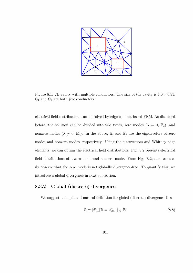
P1

C2

C1

P2

Figure 8.1: 2D cavity with multiple conductors. The size of the cavity is 1.0× 0.95.C1 and C2 are both free conductors.

electrical field distributions can be solved by edge element based FEM. As discussed

before, the solution can be divided into two types, zero modes (λ = 0, Es), and

nonzero modes (λ 6= 0, Ed). In the above, Es and Ed are the eigenvectors of zero

modes and nonzero modes, respectively. Using the eigenvectors and Whitney edge

elements, we can obtain the electrical field distributions. Fig. 8.2 presents electrical

field distributions of a zero mode and nonzero mode. From Fig. 8.2, one can eas-

ily observe that the zero mode is not globally divergence-free. To quantify this, we

introduce a global divergence in next subsection.

8.3.2 Global (discrete) divergence

We suggest a simple and natural definition for global (discrete) divergence G as

G ≡ [d∗div]D = [d∗div] [?ε]E. (8.8)

101

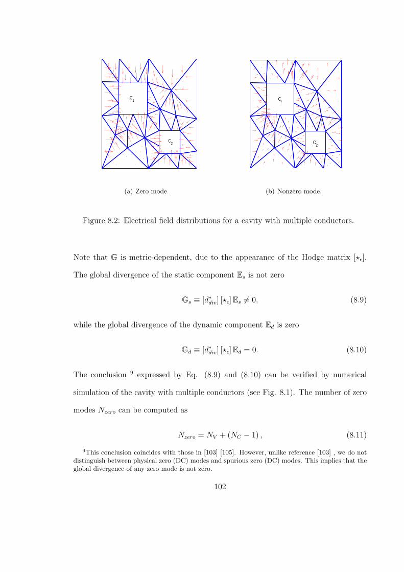
C1

C2

(a) Zero mode.

C!

C2

(b) Nonzero mode.

Figure 8.2: Electrical field distributions for a cavity with multiple conductors.

Note that G is metric-dependent, due to the appearance of the Hodge matrix [?ε].

The global divergence of the static component Es is not zero

Gs ≡ [d∗div] [?ε]Es 6= 0, (8.9)

while the global divergence of the dynamic component Ed is zero

Gd ≡ [d∗div] [?ε]Ed = 0. (8.10)

The conclusion 9 expressed by Eq. (8.9) and (8.10) can be verified by numerical

simulation of the cavity with multiple conductors (see Fig. 8.1). The number of zero

modes Nzero can be computed as

Nzero = NV + (NC − 1) , (8.11)

9This conclusion coincides with those in [103] [105]. However, unlike reference [103] , we do notdistinguish between physical zero (DC) modes and spurious zero (DC) modes. This implies that theglobal divergence of any zero mode is not zero.

102

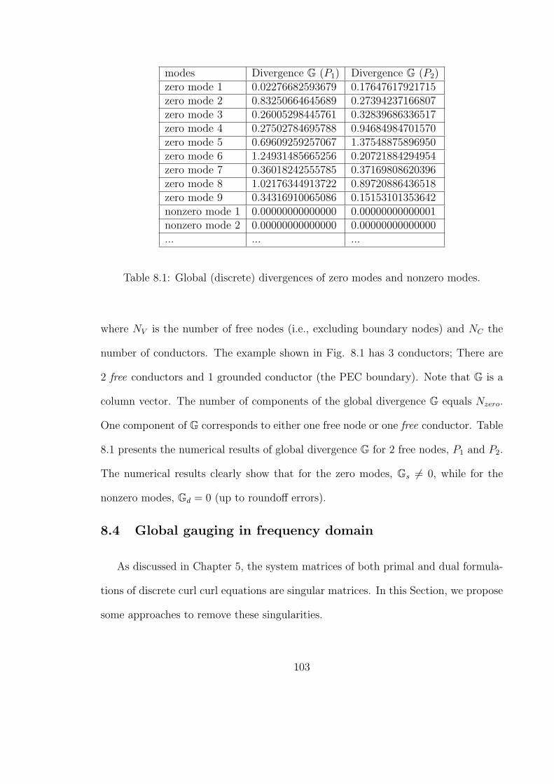
modes Divergence G (P1) Divergence G (P2)zero mode 1 0.02276682593679 0.17647617921715zero mode 2 0.83250664645689 0.27394237166807zero mode 3 0.26005298445761 0.32839686336517zero mode 4 0.27502784695788 0.94684984701570zero mode 5 0.69609259257067 1.37548875896950zero mode 6 1.24931485665256 0.20721884294954zero mode 7 0.36018242555785 0.37169808620396zero mode 8 1.02176344913722 0.89720886436518zero mode 9 0.34316910065086 0.15153101353642nonzero mode 1 0.00000000000000 0.00000000000001nonzero mode 2 0.00000000000000 0.00000000000000... ... ...

Table 8.1: Global (discrete) divergences of zero modes and nonzero modes.

where NV is the number of free nodes (i.e., excluding boundary nodes) and NC the

number of conductors. The example shown in Fig. 8.1 has 3 conductors; There are

2 free conductors and 1 grounded conductor (the PEC boundary). Note that G is a

column vector. The number of components of the global divergence G equals Nzero.

One component of G corresponds to either one free node or one free conductor. Table

8.1 presents the numerical results of global divergence G for 2 free nodes, P1 and P2.

The numerical results clearly show that for the zero modes, Gs 6= 0, while for the

nonzero modes, Gd = 0 (up to roundoff errors).

8.4 Global gauging in frequency domain

As discussed in Chapter 5, the system matrices of both primal and dual formula-

tions of discrete curl curl equations are singular matrices. In this Section, we propose

some approaches to remove these singularities.

103

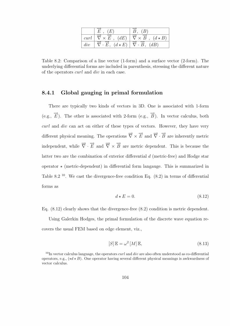
−→E , (E)

−→B , (B)

curl−→∇ ×−→E , (dE)

−→∇ ×−→B , (d ? B)

div−→∇ · −→E , (d ? E)

−→∇ · −→B , (dB)

Table 8.2: Comparison of a line vector (1-form) and a surface vector (2-form). Theunderlying differential forms are included in parenthesis, stressing the different natureof the operators curl and div in each case.

8.4.1 Global gauging in primal formulation

There are typically two kinds of vectors in 3D. One is associated with 1-form

(e.g.,−→E ). The other is associated with 2-form (e.g.,

−→B ). In vector calculus, both

curl and div can act on either of these types of vectors. However, they have very

different physical meaning. The operations−→∇ ×−→E and

−→∇ · −→B are inherently metric

independent, while−→∇ · −→E and

−→∇ × −→B are metric dependent. This is because the

latter two are the combination of exterior differential d (metric-free) and Hodge star

operator ? (metric-dependent) in differential form langauge. This is summarized in

Table 8.2 10. We cast the divergence-free condition Eq. (8.2) in terms of differential

forms as

d ? E = 0. (8.12)

Eq. (8.12) clearly shows that the divergence-free (8.2) condition is metric dependent.

Using Galerkin Hodges, the primal formulation of the discrete wave equation re-

covers the usual FEM based on edge element, viz.,

[S]E = ω2 [M ]E, (8.13)

10In vector calculus language, the operators curl and div are also often understood as co-differentialoperators, e.g., (?d ? B). One operator having several different physical meanings is awkwardness ofvector calculus.

104

when Whitney 1-forms are used as interpolants for E. In this case, this gauge (divergence-

free) condition is satisfied locally since Whitney 1-forms (cf. Chapter 2) have the local

gauging property

d ? w1i,j = 0. (8.14)

Nevertheless, the divergence-free condition Eq. (8.12) should also be satisfied globally.

Namely, the discrete solution E should obey

[d∗div] [?ε]E = 0. (8.15)

It follows that not all DoFs of E are (physically) independent. The number of Eq.

(8.15) is NV , the number of internal nodes. Thus the number of independent DoFs

of E is NE − NV , where NE is the number of internal edges. Using a tree-cotree

decomposition for the edges of the FEM mesh [99] [100], E can be split as (Et,Ec).

The Et is associated with tree edges, and Ec is associated with co-tree edges. Using

Eq. (8.15), one can express Et in terms of Ec. Thus, by eliminating Et, Eq. (8.13)

can be written as

[S]g Ec = ω2 [M ]g Ec. (8.16)

The TE modes of a rectangular cavity with size 5 × 4 (see Fig. 8.3) is computed

to demonstrate this global gauging approach. The mesh has 90 nodes, 199 internal

edges, and 144 cells. Table 8.3 presents the eigenvalues computed by Eq. (8.13)

and Eq. (8.16). The nonzero eigenvalues of Eq. (8.16) are almost same as those of

Eq. (8.13), but Eq. (8.16) has no zero modes, that is, the dimension of null space

of the system ([S]g, [M ]g) in Eq. (8.16) is zero. However, Eq. (8.16) has some

undesirable properties, viz., (i) both stiffness matrix [S]g and mass matrix [M ]g are

not symmetrical, and (ii) stiffness matrix [S]g and mass matrix [M ]g are not sparse

105

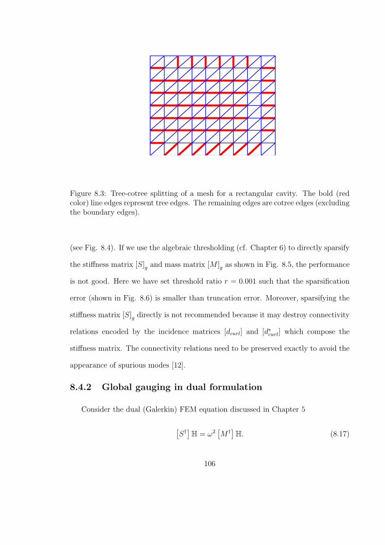
Figure 8.3: Tree-cotree splitting of a mesh for a rectangular cavity. The bold (redcolor) line edges represent tree edges. The remaining edges are cotree edges (excludingthe boundary edges).

(see Fig. 8.4). If we use the algebraic thresholding (cf. Chapter 6) to directly sparsify

the stiffness matrix [S]g and mass matrix [M ]g as shown in Fig. 8.5, the performance

is not good. Here we have set threshold ratio r = 0.001 such that the sparsification

error (shown in Fig. 8.6) is smaller than truncation error. Moreover, sparsifying the

stiffness matrix [S]g directly is not recommended because it may destroy connectivity

relations encoded by the incidence matrices [dcurl] and [d∗curl] which compose the

stiffness matrix. The connectivity relations need to be preserved exactly to avoid the

appearance of spurious modes [12].

8.4.2 Global gauging in dual formulation

Consider the dual (Galerkin) FEM equation discussed in Chapter 5

[S†

]H = ω2

[M †]H. (8.17)

106

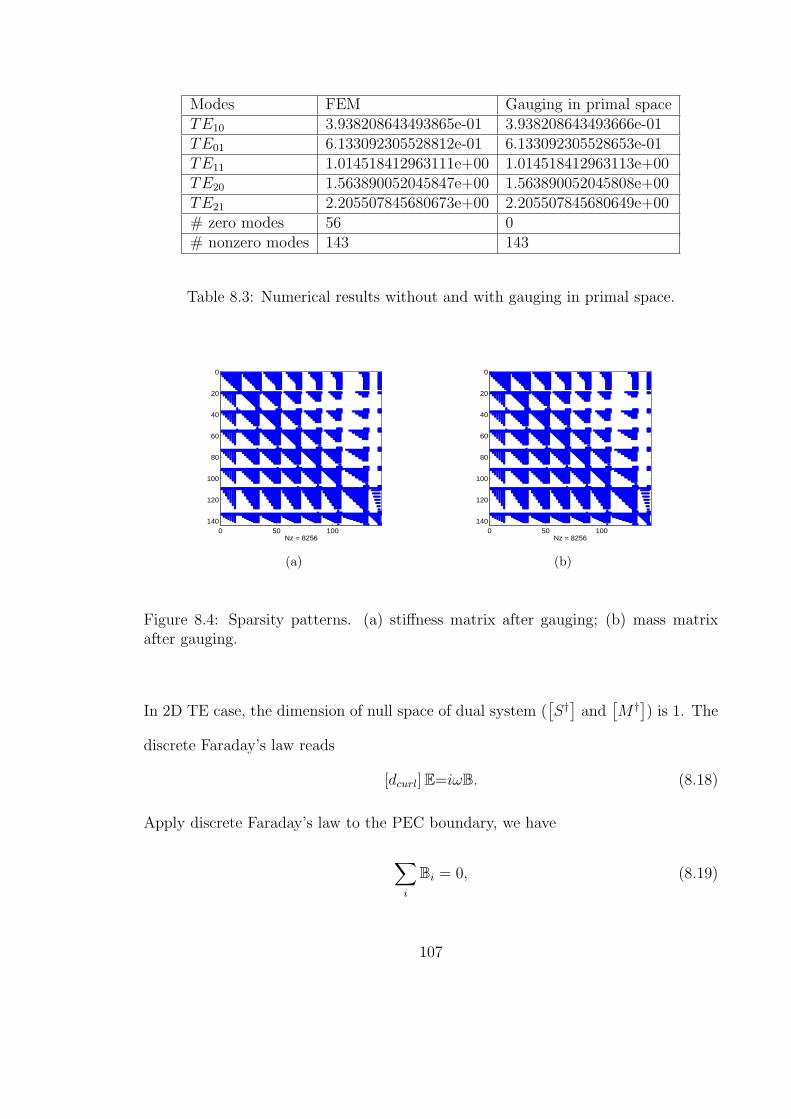
Modes FEM Gauging in primal spaceTE10 3.938208643493865e-01 3.938208643493666e-01TE01 6.133092305528812e-01 6.133092305528653e-01TE11 1.014518412963111e+00 1.014518412963113e+00TE20 1.563890052045847e+00 1.563890052045808e+00TE21 2.205507845680673e+00 2.205507845680649e+00# zero modes 56 0# nonzero modes 143 143

Table 8.3: Numerical results without and with gauging in primal space.

0 50 100

0

20

40

60

80

100

120

140

Nz = 8256

(a)

0 50 100

0

20

40

60

80

100

120

140

Nz = 8256

(b)

Figure 8.4: Sparsity patterns. (a) stiffness matrix after gauging; (b) mass matrixafter gauging.

In 2D TE case, the dimension of null space of dual system ([S†

]and

[M †]) is 1. The

discrete Faraday’s law reads

[dcurl]E=iωB. (8.18)

Apply discrete Faraday’s law to the PEC boundary, we have

∑i

Bi = 0, (8.19)

107

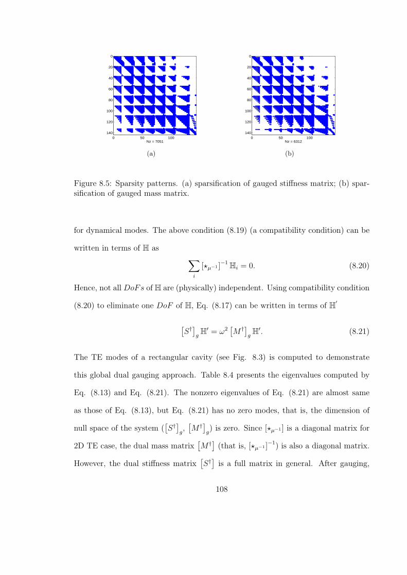
0 50 100

0

20

40

60

80

100

120

140

Nz = 7051

(a)

0 50 100

0

20

40

60

80

100

120

140

Nz = 6312

(b)

Figure 8.5: Sparsity patterns. (a) sparsification of gauged stiffness matrix; (b) spar-sification of gauged mass matrix.

for dynamical modes. The above condition (8.19) (a compatibility condition) can be

written in terms of H as∑

i

[?µ−1 ]−1Hi = 0. (8.20)

Hence, not all DoFs of H are (physically) independent. Using compatibility condition

(8.20) to eliminate one DoF of H, Eq. (8.17) can be written in terms of H′

[S†

]gH′ = ω2

[M †]

gH′. (8.21)

The TE modes of a rectangular cavity (see Fig. 8.3) is computed to demonstrate

this global dual gauging approach. Table 8.4 presents the eigenvalues computed by

Eq. (8.13) and Eq. (8.21). The nonzero eigenvalues of Eq. (8.21) are almost same

as those of Eq. (8.13), but Eq. (8.21) has no zero modes, that is, the dimension of

null space of the system ([S†

]g,[M †]

g) is zero. Since [?µ−1 ] is a diagonal matrix for

2D TE case, the dual mass matrix[M †] (that is, [?µ−1 ]−1) is also a diagonal matrix.

However, the dual stiffness matrix[S†

]is a full matrix in general. After gauging,

108

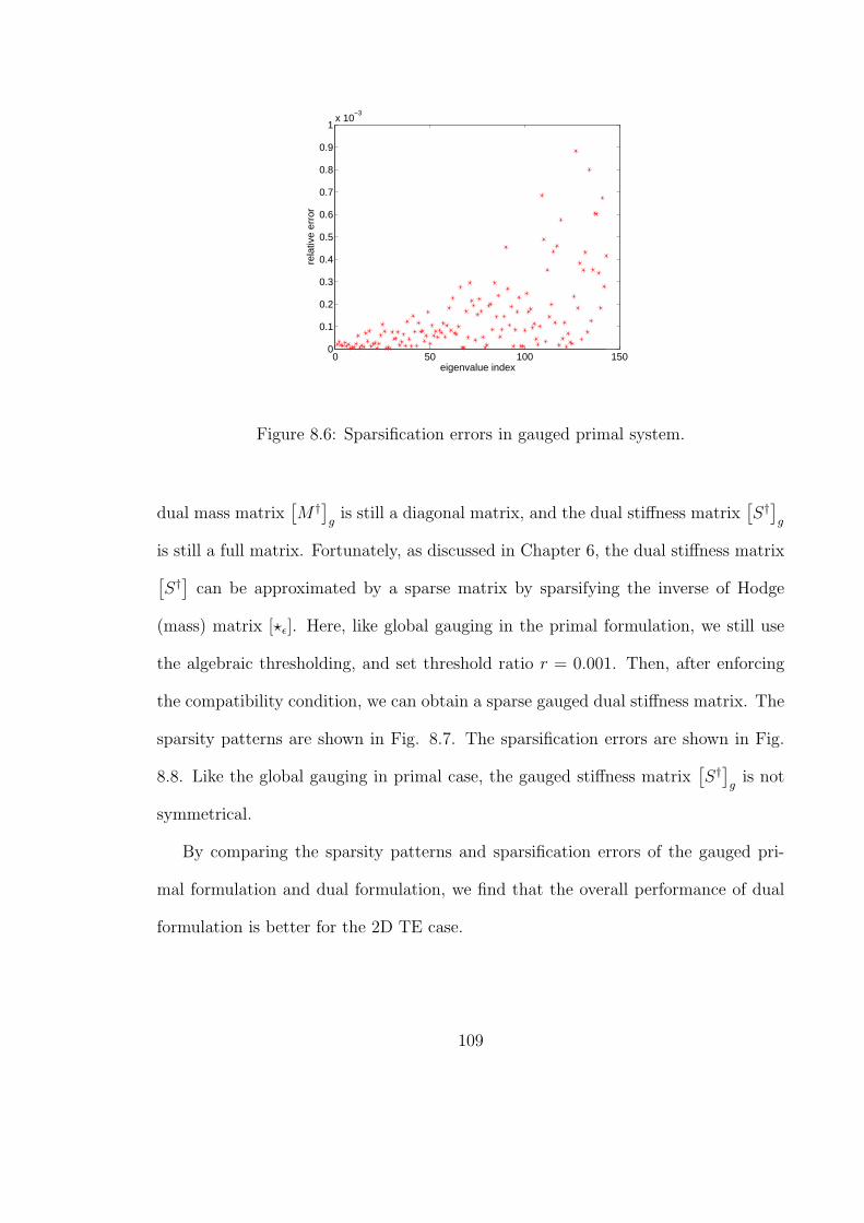
0 50 100 1500

0.1

0.2

0.3

0.4

0.5

0.6

0.7

0.8

0.9

1x 10

−3

eigenvalue index

rela

tive

erro

r

Figure 8.6: Sparsification errors in gauged primal system.

dual mass matrix[M †]

gis still a diagonal matrix, and the dual stiffness matrix

[S†

]g

is still a full matrix. Fortunately, as discussed in Chapter 6, the dual stiffness matrix

[S†

]can be approximated by a sparse matrix by sparsifying the inverse of Hodge

(mass) matrix [?ε]. Here, like global gauging in the primal formulation, we still use

the algebraic thresholding, and set threshold ratio r = 0.001. Then, after enforcing

the compatibility condition, we can obtain a sparse gauged dual stiffness matrix. The

sparsity patterns are shown in Fig. 8.7. The sparsification errors are shown in Fig.

8.8. Like the global gauging in primal case, the gauged stiffness matrix[S†

]g

is not

symmetrical.

By comparing the sparsity patterns and sparsification errors of the gauged pri-

mal formulation and dual formulation, we find that the overall performance of dual

formulation is better for the 2D TE case.

109

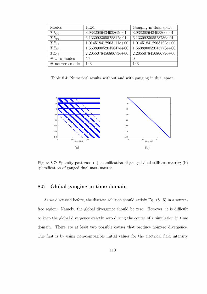
Modes FEM Gauging in dual spaceTE10 3.938208643493865e-01 3.938208643493366e-01TE01 6.133092305528812e-01 6.133092305528736e-01TE11 1.014518412963111e+00 1.014518412963122e+00TE20 1.563890052045847e+00 1.563890052045773e+00TE21 2.205507845680673e+00 2.205507845680679e+00# zero modes 56 0# nonzero modes 143 143

Table 8.4: Numerical results without and with gauging in dual space.

0 50 100

0

20

40

60

80

100

120

140

Nz = 3949

(a)

0 50 100

0

20

40

60

80

100

120

140

Nz = 143

(b)

Figure 8.7: Sparsity patterns. (a) sparsification of gauged dual stiffness matrix; (b)sparsification of gauged dual mass matrix.

8.5 Global gauging in time domain

As we discussed before, the discrete solution should satisfy Eq. (8.15) in a source-

free region. Namely, the global divergence should be zero. However, it is difficult

to keep the global divergence exactly zero during the course of a simulation in time

domain. There are at least two possible causes that produce nonzero divergence.

The first is by using non-compatible initial values for the electrical field intensity

110

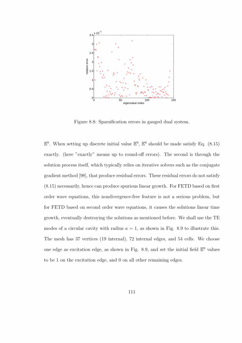
0 50 100 1500

0.5

1

1.5

2

2.5

3

3.5x 10

−3

eigenvalue index

rela

tive

erro

r

Figure 8.8: Sparsification errors in gauged dual system.

E0. When setting up discrete initial value E0, E0 should be made satisfy Eq. (8.15)

exactly. (here ”exactly” means up to round-off errors). The second is through the

solution process itself, which typically relies on iterative solvers such as the conjugate

gradient method [98], that produce residual errors. These residual errors do not satisfy

(8.15) necessarily, hence can produce spurious linear growth. For FETD based on first

order wave equations, this nondivergence-free feature is not a serious problem, but

for FETD based on second order wave equations, it causes the solutions linear time

growth, eventually destroying the solutions as mentioned before. We shall use the TE

modes of a circular cavity with radius a = 1, as shown in Fig. 8.9 to illustrate this.

The mesh has 37 vertices (19 internal), 72 internal edges, and 54 cells. We choose

one edge as excitation edge, as shown in Fig. 8.9, and set the initial field E0 values

to be 1 on the excitation edge, and 0 on all other remaining edges.

111

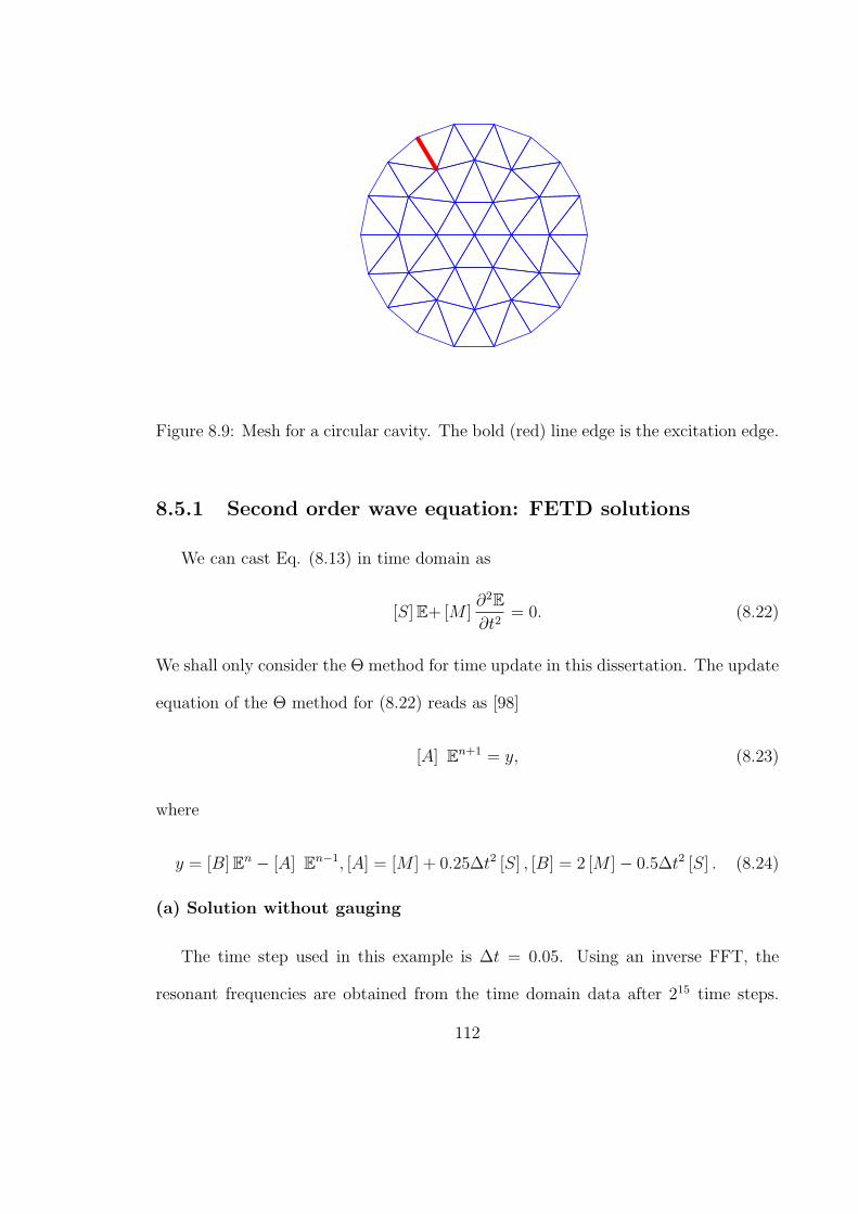
Figure 8.9: Mesh for a circular cavity. The bold (red) line edge is the excitation edge.

8.5.1 Second order wave equation: FETD solutions

We can cast Eq. (8.13) in time domain as

[S]E+ [M ]∂2E∂t2

= 0. (8.22)

We shall only consider the Θ method for time update in this dissertation. The update

equation of the Θ method for (8.22) reads as [98]

[A] En+1 = y, (8.23)

where

y = [B]En − [A] En−1, [A] = [M ] + 0.25∆t2 [S] , [B] = 2 [M ]− 0.5∆t2 [S] . (8.24)

(a) Solution without gauging

The time step used in this example is ∆t = 0.05. Using an inverse FFT, the

resonant frequencies are obtained from the time domain data after 215 time steps.

112

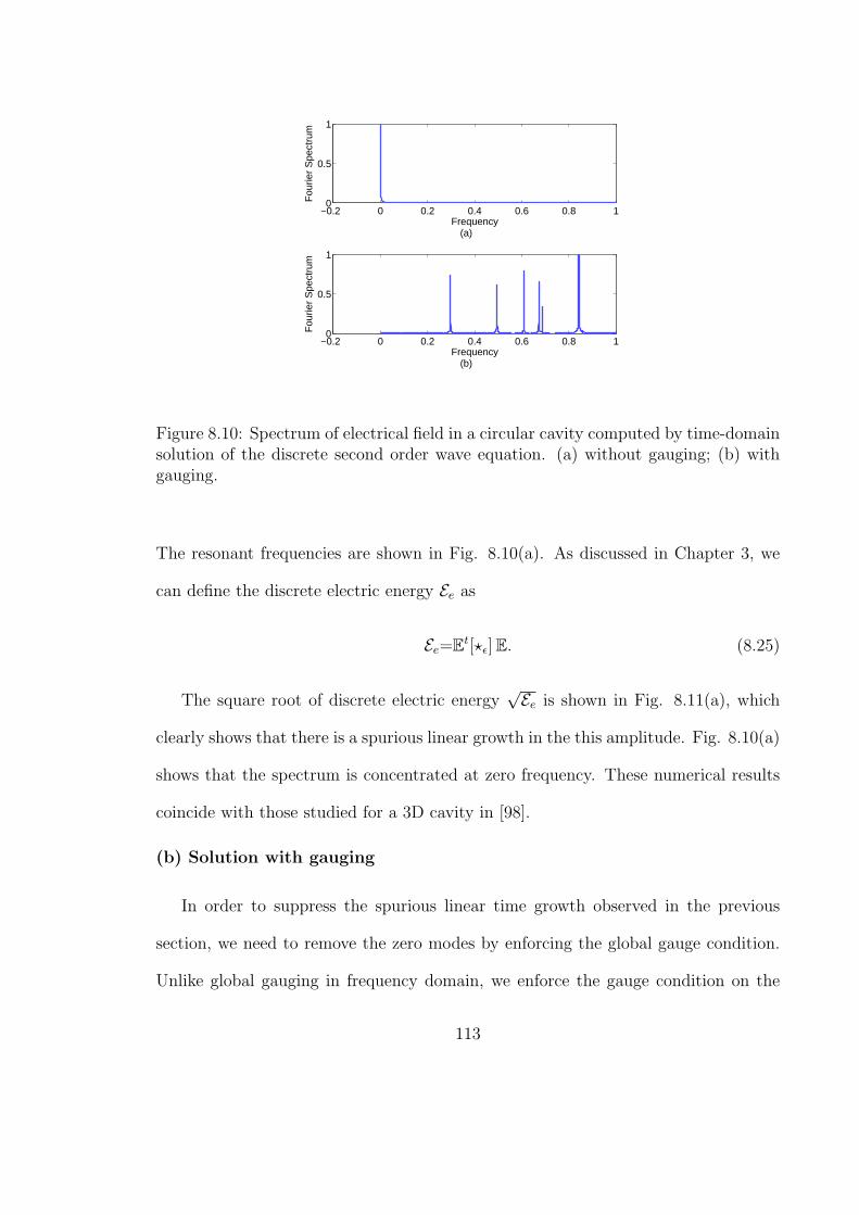
−0.2 0 0.2 0.4 0.6 0.8 10

0.5

1

Frequency(a)

Fou

rier

Spe

ctru

m

−0.2 0 0.2 0.4 0.6 0.8 10

0.5

1

Frequency(b)

Fou

rier

Spe

ctru

m

Figure 8.10: Spectrum of electrical field in a circular cavity computed by time-domainsolution of the discrete second order wave equation. (a) without gauging; (b) withgauging.

The resonant frequencies are shown in Fig. 8.10(a). As discussed in Chapter 3, we

can define the discrete electric energy Ee as

Ee=Et[?ε]E. (8.25)

The square root of discrete electric energy√Ee is shown in Fig. 8.11(a), which

clearly shows that there is a spurious linear growth in the this amplitude. Fig. 8.10(a)

shows that the spectrum is concentrated at zero frequency. These numerical results

coincide with those studied for a 3D cavity in [98].

(b) Solution with gauging

In order to suppress the spurious linear time growth observed in the previous

section, we need to remove the zero modes by enforcing the global gauge condition.

Unlike global gauging in frequency domain, we enforce the gauge condition on the

113

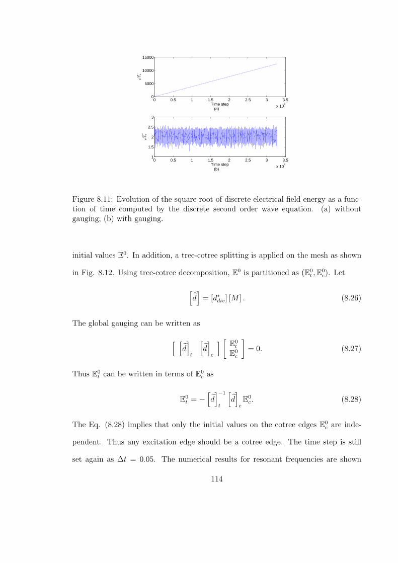
0 0.5 1 1.5 2 2.5 3 3.5

x 104

0

5000

10000

15000

√E e

Time step(a)

0 0.5 1 1.5 2 2.5 3 3.5

x 104

1

1.5

2

2.5

3

√E e

Time step(b)

Figure 8.11: Evolution of the square root of discrete electrical field energy as a func-tion of time computed by the discrete second order wave equation. (a) withoutgauging; (b) with gauging.

initial values E0. In addition, a tree-cotree splitting is applied on the mesh as shown

in Fig. 8.12. Using tree-cotree decomposition, E0 is partitioned as (E0t ,E0

c). Let

[d]

= [d∗div] [M ] . (8.26)

The global gauging can be written as

[ [d]

t

[d]

c

] [E0

t

E0c

]= 0. (8.27)

Thus E0t can be written in terms of E0

c as

E0t = −

[d]−1

t

[d]

cE0

c . (8.28)

The Eq. (8.28) implies that only the initial values on the cotree edges E0c are inde-

pendent. Thus any excitation edge should be a cotree edge. The time step is still

set again as ∆t = 0.05. The numerical results for resonant frequencies are shown

114

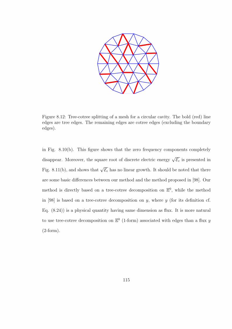
Figure 8.12: Tree-cotree splitting of a mesh for a circular cavity. The bold (red) lineedges are tree edges. The remaining edges are cotree edges (excluding the boundaryedges).

in Fig. 8.10(b). This figure shows that the zero frequency components completely

disappear. Moreover, the square root of discrete electric energy√Ee is presented in

Fig. 8.11(b), and shows that√Ee has no linear growth. It should be noted that there

are some basic differences between our method and the method proposed in [98]. Our

method is directly based on a tree-cotree decomposition on E0, while the method

in [98] is based on a tree-cotree decomposition on y, where y (for its definition cf.

Eq. (8.24)) is a physical quantity having same dimension as flux. It is more natural

to use tree-cotree decomposition on E0 (1-form) associated with edges than a flux y

(2-form).

115

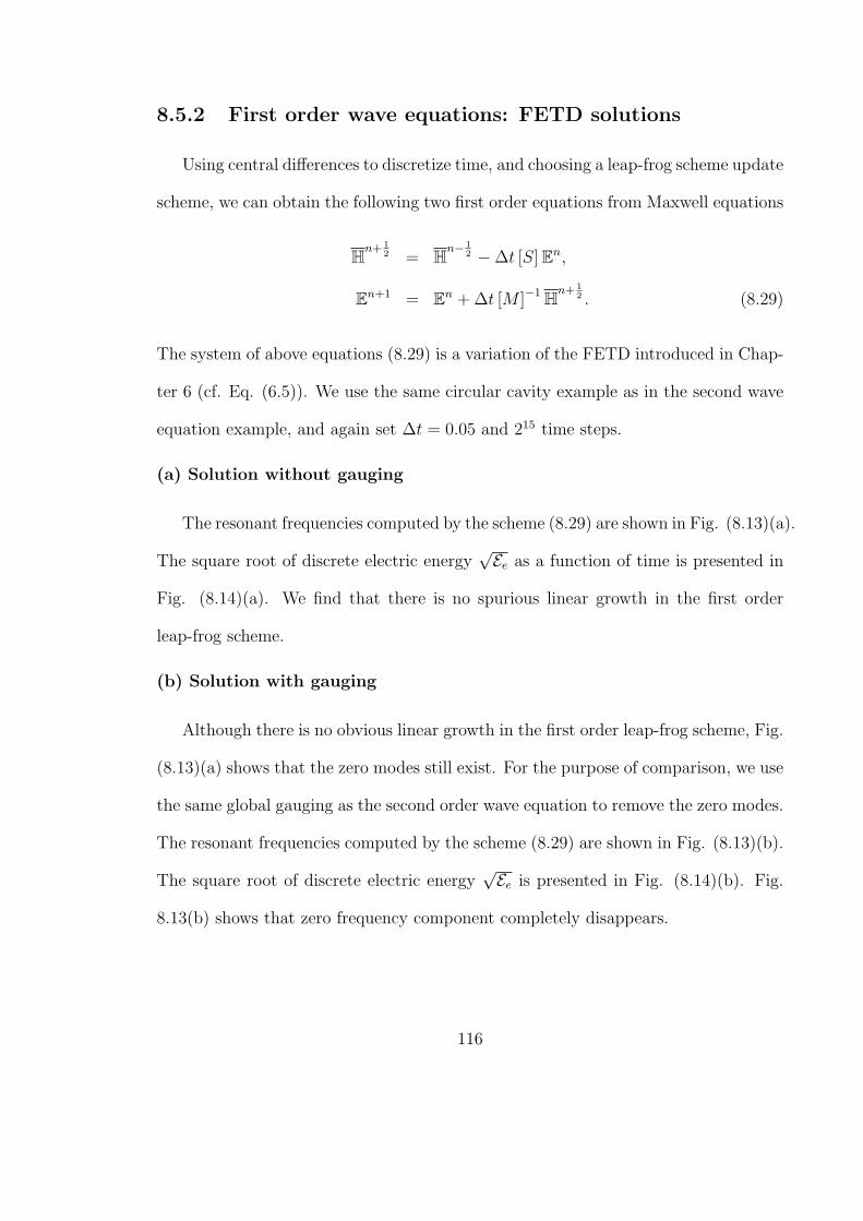
8.5.2 First order wave equations: FETD solutions

Using central differences to discretize time, and choosing a leap-frog scheme update

scheme, we can obtain the following two first order equations from Maxwell equations

Hn+ 12 = Hn− 1

2 −∆t [S]En,

En+1 = En + ∆t [M ]−1Hn+ 12 . (8.29)

The system of above equations (8.29) is a variation of the FETD introduced in Chap-

ter 6 (cf. Eq. (6.5)). We use the same circular cavity example as in the second wave

equation example, and again set ∆t = 0.05 and 215 time steps.

(a) Solution without gauging

The resonant frequencies computed by the scheme (8.29) are shown in Fig. (8.13)(a).

The square root of discrete electric energy√Ee as a function of time is presented in

Fig. (8.14)(a). We find that there is no spurious linear growth in the first order

leap-frog scheme.

(b) Solution with gauging

Although there is no obvious linear growth in the first order leap-frog scheme, Fig.

(8.13)(a) shows that the zero modes still exist. For the purpose of comparison, we use

the same global gauging as the second order wave equation to remove the zero modes.

The resonant frequencies computed by the scheme (8.29) are shown in Fig. (8.13)(b).

The square root of discrete electric energy√Ee is presented in Fig. (8.14)(b). Fig.

8.13(b) shows that zero frequency component completely disappears.

116

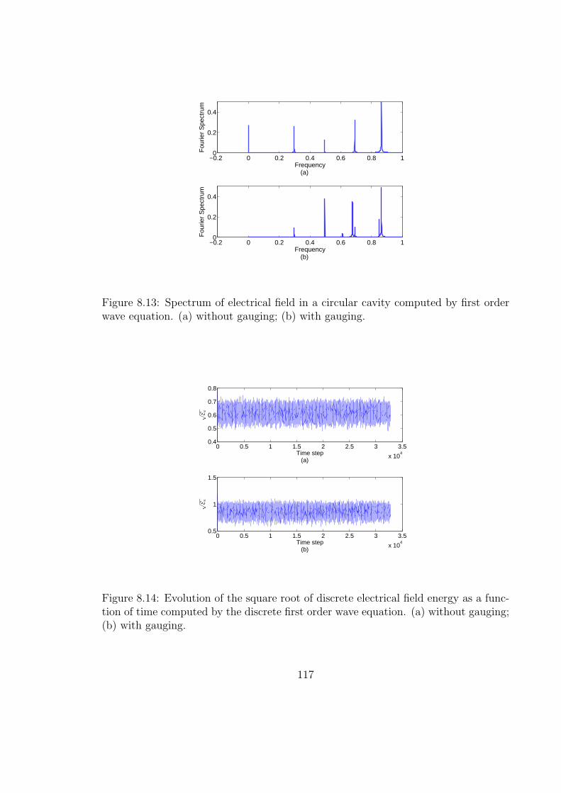
−0.2 0 0.2 0.4 0.6 0.8 10

0.2

0.4

Frequency(a)

Fou

rier

Spe

ctru

m

−0.2 0 0.2 0.4 0.6 0.8 10

0.2

0.4

Frequency(b)

Fou

rier

Spe

ctru

m

Figure 8.13: Spectrum of electrical field in a circular cavity computed by first orderwave equation. (a) without gauging; (b) with gauging.

0 0.5 1 1.5 2 2.5 3 3.5

x 104

0.4

0.5

0.6

0.7

0.8

√E e

Time step(a)

0 0.5 1 1.5 2 2.5 3 3.5

x 104

0.5

1

1.5

√E e

Time step(b)

Figure 8.14: Evolution of the square root of discrete electrical field energy as a func-tion of time computed by the discrete first order wave equation. (a) without gauging;(b) with gauging.

117


To conclude this chapter, we offer some additional remarks.

Remark 1 : The concept of global (discrete) divergence can also be used for the

singularity of magnetostatic problem if the vector potential−→A is used to solve the

curl curl equation

−→∇ × 1

µ

−→∇ ×−→A =−→J , (8.30)

where−→J the external (impressed) current density.

Remark 2 : We have not addressed here computational cost issues of global gaug-

ing techniques (e.g., partitioning a mesh into tree edges and cotree edges, obtaining

inverse of[d]

tin Eq. (8.28), etc.). These will be a topic of a future work.

118

CHAPTER 9

CONCLUSIONS

The main goal of this work has been to develop and study reliable, stable, and

efficient numerical techniques to solve Maxwell equations in irregular lattices (grids).

This has been achieved by means of compatible discretizations. Compatible is defined

as that numerical solutions that capture the essential physical properties of Maxwell

equation without spurious solutions. It should be mentioned that although the basic

philosophy of compatible discretizations has been around for a long time [106] [14],

and has attracted renewed interests recently [107] [108]. We next summarize the most

important contributions in this dissertation.

By applying some tools of algebraic topology and discrete differential forms, gen-

eral compatible discretizations for Maxwell equations (also called discrete Maxwell

equations) can be obtained in an arbitrary network of polygons for 2D (polyhedra for

3D). For discrete Maxwell equations, we have shown that Euler’s formula matches the

algebraic properties of the discrete Hodge decomposition in an exact way. Further-

more, we have shown that discrete Maxwell equations satisfy the following identity

DoF d (E) = DoF d (B) = DoF d (D) = DoF d (H) , (9.1)

that is, the number of dynamic DoFs is the same for all 1-form and 2-form fields.

The identity (9.1) reflects an essential algebraic property discrete Maxwell equations.

119

All algorithms developed in this work observe the identity (9.1) exactly. We have

also discussed how to discretize (metric-dependent) constitutive equations by means

of discrete Hodge operators. In the FEM case, we have used Galerkin Hodges as

discrete Hodge operators.

We have unveiled a new duality for (discrete) Maxwell equations, denoted as

Galerkin duality. This duality is a mathematical transformation between two (dual)

system matrices, [XE] (primal formulation) and [XH ] (dual formulation) respectively

that discretize Maxwell equations. We have shown that the primal formulation re-

covers the conventional (edge-element) finite element method (FEM) and suggests

a geometric viewpoint for it. On the other hand, the dual formulation suggests a

new (dual) type of FEM. Since both formulations describe same discrete physical

system, they should produce same dynamical solutions. However, their null spaces

are different. The global features of both have been studied using a discrete version of

the Hodge decomposition and Euler’s formula for a network of polygons for 2D case

and polyhedra for 3D case. All these have been verified by numerical simulations of

several canonical 2D and 3D cases.

We have found that despite being full matrices, the inverse Hodge matrices have

strong localization properties. Therefore, they can be sparsified efficiently with neg-

ligible loss of accuracy. We have proposed two thresholding techniques, algebraic

thresholding and topological thresholding to sparsify inverse Hodge matrices. Based

on these thresholding techniques, we have developed and implemented a sparse and

fully explicit FETD. This scheme is quite similar to FDTD, that is, updating for each

unknown only requires neighboring nodes and/or edges, but can be applied to general

irregular grids. We would like to point out that the topological thresholding technique

120

also provides a very general and systematic way to derive stable local finite-difference

stencils in irregular grids. These stencils are, of course, grid-dependent.

We have proposed to a mixed FEM scheme for Maxwell equations. This scheme

is based on using the electric field intensity−→E and magnetic field flux

−→B (instead

of magnetic field intensity−→H ) as the state variables such that it results in sparse

matrices. Several numerical examples including photonic crystals have demonstrated

the effectiveness of this scheme.

Motivated by low-frequency instability problems in frequency domain FEM and

the spurious linear growth problem in time domain FEM, we have analyzed the sin-

gular nature of FEM matrices arising from the null spaces of curl operators. We

have introduced global divergences and global gauging to handle low-frequency in-

stability and spurious solutions linear growth problems. Our techniques are based

on a tree-cotree decomposition of a mesh. The tree-cotree decomposition of a mesh

(graph) only depends on the topology (connectivity) of the mesh. However, we have

emphasized that any exact gauging (cf. Eq. (8.8)) should also depend on metric

information. Several numerical examples both in frequency domain and time domain

show the effectiveness of our techniques.

121

APPENDIX A

STIFFNESS MATRICES: GEOMETRIC VIEWPOINT

Using 3D tetrahedral and cubic elements, respectively, and assuming that the

permeability µ is constant within each element, we will show that stiffness matrix [S]

equals the multiplication of incidences and Hodge matrices

[S] = [d∗curl] [?µ−1 ] [dcurl] . (A.1)

As discussed in Section 5.2, since the (global) mass matrix and stiffness matrix can be

obtained by direct summation (assemblation) of (local) mass matrices and stiffness

matrices, relation (A.1) only needs to be shown on a single generic element. Hence,

in this Appendix, the integration is carried out on a single element.

A.1 Tetrahedral element

From the DoFs for the tetrahedral element (Fig. A.1)

B =[

b1,2,3 b1,3,4 b1,4,2 b2,4,3

]t, (A.2)

E =[

e1,2 e1,3 e1,4 e2,3 e4,2 e3,4

]t, (A.3)

122

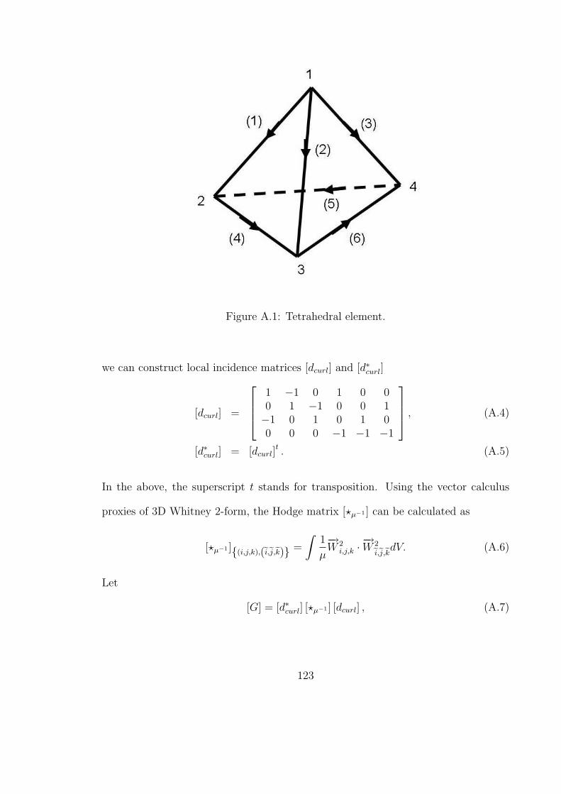
Figure A.1: Tetrahedral element.

we can construct local incidence matrices [dcurl] and [d∗curl]

[dcurl] =

1 −1 0 1 0 00 1 −1 0 0 1−1 0 1 0 1 00 0 0 −1 −1 −1

, (A.4)

[d∗curl] = [dcurl]t . (A.5)

In the above, the superscript t stands for transposition. Using the vector calculus

proxies of 3D Whitney 2-form, the Hodge matrix [?µ−1 ] can be calculated as

[?µ−1 ](i,j,k),(ei,ej,ek) =

∫1

µ

−→W 2

i,j,k ·−→W 2ei,ej,ekdV. (A.6)

Let

[G] = [d∗curl] [?µ−1 ] [dcurl] , (A.7)

123

which is a 6× 6 matrix. The entry of local stiffness matrix [S] can be computed as

[S](i,j),(ei,ej) =

∫1

µ

(−→∇ ×−→W 1i,j

)·(−→∇ ×−→W 1

ei,ej

)dV

=1

µ

(2−→∇ζi ×−→∇ζj

)·(2−→∇ζei ×

−→∇ζej)

. (A.8)

By comparing each term of matrix (A.7) with the corresponding term of matrix (A.8),

such as [G]12

[G]12 = − [?µ−1 ]11

+ [?µ−1 ]31

+ [?µ−1 ]12− [?µ−1 ]

32(A.9)

=1

µ

(2−→∇ζ1 ×−→∇ζ2

)·(2−→∇ζe1 ×

−→∇ζe3)

, (A.10)

and [S]12

[S]12 =1

µ

(2−→∇ζ1 ×−→∇ζ2

)·(2−→∇ζe1 ×

−→∇ζe3)

, (A.11)

we obtain

[S] = [d∗curl] [?µ−1 ] [dcurl] . (A.12)

A.2 Cubic element

Consider a cubic element given in Fig. A.2, whose side length is L and whose

center is at (xc, yc). From the DoFs for the cubic element

B =[

b1,4,3,2 b5,6,7,8 b2,3,7,6 b1,5,8,4 b1,2,6,5 b3,4,8,7

]t, (A.13)

E =[

e1,2 e4,3 e5,6 e8,7 e1,4 e5,8 e2,3 e6,7 e1,5 e2,6 e4,8 e3,7

]t, (A.14)

we can construct the local incidence matrix [dcurl] and [d∗curl] for the cubic element

[dcurl] =

−1 1 1 −11 −1 −1 1

1 −1 −1 1−1 1 1 −1

1 −1 −1 1−1 1 1 −1

, (A.15)

124

[d∗curl] = [dcurl]t . (A.16)

The edge elements−→N 1

i,j for a cubic element can be written as [3] 11

−→N 1

1,2 =1

L3

(yc +

L

2− y

)(zc +

L

2− z

)x,

−→N 1

4,3 =1

L3

(−yc +

L

2+ y

)(zc +

L

2− z

)x,

−→N 1

5,6 =1

L3

(yc +

L

2− y

)(−zc +

L

2+ z

)x,

−→N 1

8,7 =1

L3

(−yc +

L

2+ y

)(−zc +

L

2+ z

)x,

−→N 1

1,4 =1

L3

(zc +

L

2− z

) (xc +

L

2− x

)y,

−→N 1

5,8 =1

L3

(−zc +

L

2+ z

)(xc +

L

2− x

)y,

−→N 1

2,3 =1

L3

(zc +

L

2− z

) (−xc +

L

2+ x

)y,

−→N 1

6,7 =1

L3

(−zc +

L

2+ z

)(−xc +

L

2+ x

)y,

−→N 1

1,5 =1

L3

(xc +

L

2− x

)(yc +

L

2− y

)z,

−→N 1

2,6 =1

L3

(−xc +

L

2+ x

)(yc +

L

2− y

)z,

−→N 1

4,8 =1

L3

(xc +

L

2− x

)(−yc +

L

2+ y

)z,

−→N 1

3,7 =1

L3

(−xc +

L

2+ x

)(−yc +

L

2+ y

)z. (A.17)

The corresponding face elements−→N 2

i,j,k,l can be constructed as

11The normalizations used here are different from those of [3].

125

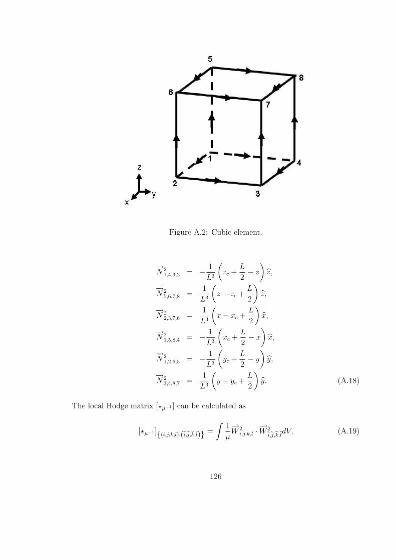
Figure A.2: Cubic element.

−→N 2

1,4,3,2 = − 1

L3

(zc +

L

2− z

)z,

−→N 2

5,6,7,8 =1

L3

(z − zc +

L

2

)z,

−→N 2

2,3,7,6 =1

L3

(x− xc +

L

2

)x,

−→N 2

1,5,8,4 = − 1

L3

(xc +

L

2− x

)x,

−→N 2

1,2,6,5 = − 1

L3

(yc +

L

2− y

)y,

−→N 2

3,4,8,7 =1

L3

(y − yc +

L

2

)y. (A.18)

The local Hodge matrix [?µ−1 ] can be calculated as

[?µ−1 ](i,j,k,l),(ei,ej,ek,el) =

∫1

µ

−→W 2

i,j,k,l ·−→W 2ei,ej,ek,eldV, (A.19)

126

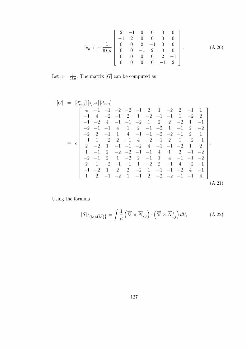
[?µ−1 ] =1

6Lµ

2 −1 0 0 0 0−1 2 0 0 0 00 0 2 −1 0 00 0 −1 2 0 00 0 0 0 2 −10 0 0 0 −1 2

. (A.20)

Let c = 16Lµ

. The matrix [G] can be computed as

[G] = [d∗curl] [?µ−1 ] [dcurl]

= c

4 −1 −1 −2 −2 −1 2 1 −2 2 −1 1−1 4 −2 −1 2 1 −2 −1 −1 1 −2 2−1 −2 4 −1 −1 −2 1 2 2 −2 1 −1−2 −1 −1 4 1 2 −1 −2 1 −1 2 −2−2 2 −1 1 4 −1 −1 −2 −2 −1 2 1−1 1 −2 2 −1 4 −2 −1 2 1 −2 −12 −2 1 −1 −1 −2 4 −1 −1 −2 1 21 −1 2 −2 −2 −1 −1 4 1 2 −1 −2−2 −1 2 1 −2 2 −1 1 4 −1 −1 −22 1 −2 −1 −1 1 −2 2 −1 4 −2 −1−1 −2 1 2 2 −2 1 −1 −1 −2 4 −11 2 −1 −2 1 −1 2 −2 −2 −1 −1 4

.

(A.21)

Using the formula

[S](i,j),(ei,ej) =

∫1

µ

(−→∇ ×−→N 1i,j

)·(−→∇ ×−→N 1

ei,ej

)dV, (A.22)

127

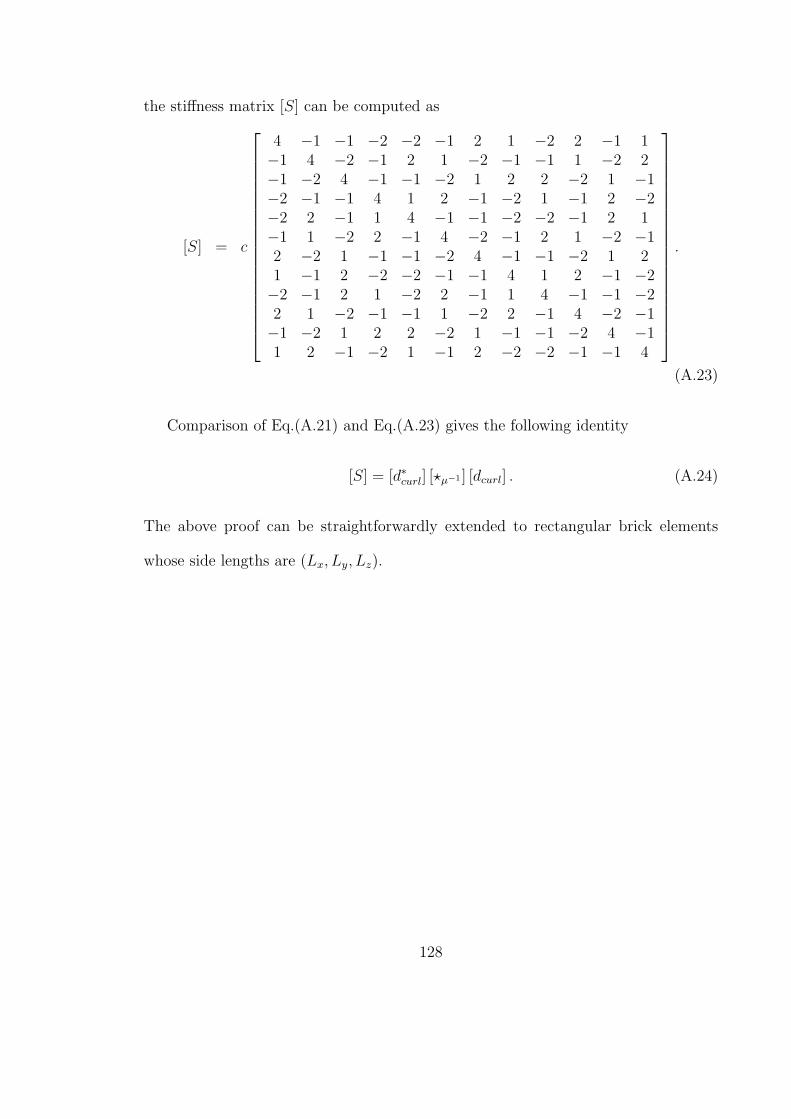
the stiffness matrix [S] can be computed as

[S] = c

4 −1 −1 −2 −2 −1 2 1 −2 2 −1 1−1 4 −2 −1 2 1 −2 −1 −1 1 −2 2−1 −2 4 −1 −1 −2 1 2 2 −2 1 −1−2 −1 −1 4 1 2 −1 −2 1 −1 2 −2−2 2 −1 1 4 −1 −1 −2 −2 −1 2 1−1 1 −2 2 −1 4 −2 −1 2 1 −2 −12 −2 1 −1 −1 −2 4 −1 −1 −2 1 21 −1 2 −2 −2 −1 −1 4 1 2 −1 −2−2 −1 2 1 −2 2 −1 1 4 −1 −1 −22 1 −2 −1 −1 1 −2 2 −1 4 −2 −1−1 −2 1 2 2 −2 1 −1 −1 −2 4 −11 2 −1 −2 1 −1 2 −2 −2 −1 −1 4

.

(A.23)

Comparison of Eq.(A.21) and Eq.(A.23) gives the following identity

[S] = [d∗curl] [?µ−1 ] [dcurl] . (A.24)

The above proof can be straightforwardly extended to rectangular brick elements

whose side lengths are (Lx, Ly, Lz).

128

BIBLIOGRAPHY

[1] K. S. Yee, “Numerical solution of initial boundary value problems involvingMaxwell’s equations in isotropic media,” IEEE Trans. Antennas and Propagat.,vol. 14, pp. 302-307, 1966.

[2] A. Taflove and S. Hagness, Computational Electromagnetics, The finite Differ-ence Time Domain Method, Second Edition, Artech, Boston, 2000.

[3] J. M. Jin, The Finite Element Method in Electromagnetics, Wiley, New York,2002.

[4] J. L. Volakis, A. Chatterjee, and L. C. Kempel, Finite Element Method forElectromagnetics: Antennas, Microwave Circuits, and Scattering Applications,IEEE Press, New York, 1998.

[5] R. Hiptmair, “Finite elements in computational electromagnetism,”Acta Nu-merica, vol. 11, pp. 237-339, 2002.

[6] P. Monk, Finite Element methods for Maxwell’s Equations, Oxford UniversityPress, Oxford, 2003.

[7] A. Bossavit, Computational Electromagnetism, Academic Press, San Diego,1998.

[8] A. Bossavit, “Solving Maxwell equations in a closed cavity, and the question of“spurious modes”,” IEEE Tran. On Magn., vol. 26, pp. 702-705, 1990.

[9] D. Sun, et al., “Spurious modes in finite element methods,” IEEE Trans. An-tennas and Propagat., vol. 37, pp. 12-24, 1995.

[10] R.Schuhmann and T. Weiland, “Stability of the FDTD algorithm on nonorthog-onal grids related to the spatial interpolation scheme,” IEEE Trans. Magn., vol.34, pp. 2751-2754, 1998.

[11] J. -F. Lee, D. K. Sun, and Z. J. Cendes, “Tangential vector finite elements forelectromagnetic field computation,” IEEE Trans. Magn., vol, 27, pp. 4032-4035,1991.

129

[12] F. L. Teixeira and W. C. Chew, “Lattice electromagnetic theory from a topo-logical viewpoint,” J. Math. Phys. vol. 40, pp. 169-187, 1999.

[13] F. L. Teixeira, Geometric Methods for Computational Electromagnetics, PIER32, EMW Publishing, Cambridge, Mass., 2001.

[14] J. M. Hyman and M. Shashkov, “Mimetic discretizations for Maxwell’s equa-tions,” J. Comput. Phys. vol. 151, pp. 881-909, 1999.

[15] T. Weiland, “A discretization method for the solution of Maxwell’s Equationsfor six-component field,” Electronics and Communications AEU, vol. 31, no. 3,pp. 116-120, 1977.

[16] H. Flanders, Differertial Forms with Applications to the Physical Sciences,Dover, New York, 1989.

[17] T. Frankel, The Geometry of Physics: an Introduction, Cambridge UniversityPress, Cambridge, UK, 2004

[18] C. V. Westenholz, Differential Forms in Mathematical Physics, Elsevier Science,North-Holland, 1980.

[19] W. L. Burke, Applied Differential Geometry, Cambridge University Press, NewYork, 1985.

[20] R. W. R. Darling, Differential Forms and Connections, Cambridge UniversityPress, Cambridge, 1994.

[21] G. A. Deschamps, “Electromagnetics and differential forms,” IEEE Proc. , vol.69, pp. 676-696, 1981.

[22] K. F. Warnick, R. H. Selfridge, and D. V. Arnold, “Teaching electromagneticfield theory using differential forms,” IEEE Trans. Educ., vol. 40, pp. 53-68,1997.

[23] P. W. Gross and P. R. Kotiuga, Electromagnetic Theory and Computation: ATopological Approach, Cambridge University Press, Cambridge, 2004.

[24] P. Russer, Electromagnetics, Microwave Circuit and Antenna Design for Com-munications Engineering, Artech, Boston, 2003.

[25] I. V. Lindell, Differential Forms in Electromagnetics, A John Wiley & Sons,Inc. Publication, 2004.

[26] D. Baldomir, “Differential forms and electromagnetism in 3-dimensional Eu-clidean space R3,” IEE Proc. A 133, pp. 139-143, 1986.

130

[27] W. H. Whitney, Geometric Integration Theory, Princeton University Press,Princeton, 1957.

[28] G. de Rham, Differential manifolds: Forms, currents, harmonic forms, Englishedition, Springer-Verlag, Berlin Heidelberg, 1984.

[29] J. R. Munkres, Elements of Algebraic Topology, Addison-Wesley, Reading, MA,1984.

[30] T. J. Honan, “The geometry of lattice field theory,” Ph.D. thesis, University ofMaryland, 1986.

[31] M. Desbrun, E. Kanso, and Y. Tong “Discrete differential forms for computa-tional modeling,” Chapter in ACM SIGGRAPH’05 Course Notes on DiscreteDifferential Geometry.

[32] A. N. Hirani, “Discrete exterior calculus,” Ph.D. thesis, California Institute ofTechnology, 2003.

[33] M. Desbrun, A. N. Hirani, M. Leok, and J. Marsden, “Discrete exterior calcu-lus,” arXiv, math.DG/0508341, 2005.

[34] C. Mattiussi, “The finite volume, finite difference, and finite element methodsusing some concepts from algebraic topology,” J. Comput. Phys., vol. 133, pp.289-309, 1997.

[35] Andre Weil, “Sur les theoremes de de Rham,” Comment. Math. Helv. vol. 26,pp.119-145, 1952.

[36] R. Adams, Sobolev Spaces, Acasemic Press, New York, 1975.

[37] J. J. Sakurai, Modern Quantum Mechanics, The Benjamin/Cummings Publish-ing Company, Menlo Park, 1985.

[38] R. Shankar, Principles of Quantum Mechanics, Second Edition, Plenum Press,New York, 1994.

[39] A. Bossavit, “(4): From degrees of freedom to fields,” J. Japan Soc. Appl.Electromagn. & Mech., A, vol 8, pp. 102-109, 2000.

[40] A. Bossavit, “(5): The “Galerkin hodge”,” J. Japan Soc. Appl. Electromagn.& Mech., A, vol 8, pp. 203-209, 2000.

[41] A. Bossavit, “Generating Whitney forms of polynomial degree one and higher,”IEEE Tran. Magn., vol. 38, no. 2, pp. 314-344, 2000.

131

[42] P. R. Raviart and J. M. Thomas, “A mixed finite element method for secondoeder elliptical problems,” vol. 606, Springer Lecture Notes in Mathematics,Springer, New York, pp. 292-315, 1977.

[43] J. Nedelec, “Mixed finite elements in R3,” Numer. Math. vol. 35, pp. 315-341,1980.

[44] J. Nedelec, “A new family of mixed finite elements in R3,” Numer. Math. vol.50, pp. 57-81, 1986.

[45] V. Girault and P. Raviart, Finite Element Methods for Navier-Stokes Equations,Springer, Berlin, 1986.

[46] S. M. Rao, D. R. Wilton, and A. W. Glisson,“Electromagnetic scattering by ar-bitrarily shaped three dimensional homogeneous lossy dielectric objects,”IEEETrans. Antennas Propag., vol. 30, pp. 409-418, 1982.

[47] M. L. Barton and Z. J. Cendes, “New vector finite elements for three-dimensional magnetic field computation,”J. Appl. Phys., vol. 61, no. 8, pp. 3919-3921, 1987.

[48] A. Bossavit, “Whitney forms: a class of finite elements for three-dimensionalcomputations in electromagnetism,” IEE Proc., vol. 135, A, no. 8, pp. 493-500,1988.

[49] D. H. Adams, “A double discretization of Abelian Chern-Simons theory,” Phys.Rev. Lett., vol. 78, pp. 4155-4158, 1997.

[50] S. Sen, et al., “Geometric discretization scheme applied to the Abelian Chern-Simons theory,” Phys. Rev. E. vol. 61, pp. 3174-3185, 2000.

[51] J. H. Rabin, “Homology theory of lattice fermion doubling,” Nucl. Phys. B, vol.201, pp. 315-332, 1982.

[52] R. Rieben, D. White and G. Rodrigue, “High order symplectic integration meth-ods for finite element solutions to time dependent Maxwell equations,” IEEETrans. Antennas Propagat. vol. 52, pp. 2190-2195, 2004.

[53] D. N. Arnold, “Differential complexes and numerical stability,” in Proceedingsof the International Congress of Mathematicians, Volume 1: Plenary Lectures,pp. 137-157, Beijing, China, 2002.

[54] V. Gradinaru and R. Hiptmair, “Whitney elements on pyramids,” Electron.Trans. Numer. Anal. vol. 8, pp. 154-168, 1999.

132

[55] T. Rylander and A. Bondeson, “Stable FEM-FDTD hybrid method forMaxwell’s equations,” Comput. Phys. Commun., vol. 125, pp. 75-82, 2000.

[56] R. Hiptmair, “From E to Edge Elements,” The Academician, vol. 3, pp. 23-31,2003.

[57] E. Tonti, “Finite Formulation of the Electromagnetic Field,” in GeometricMethods for Computational Electromagnetics (PIER Series 32, F. L. Teixeira,ed.), EMW Publishing, Cambridge, pp. 1-44, 2001.

[58] A. Bossavit and L. Kettunen, “Yee-like schemes on staggered cellulars grids: Asynthesis between FIT and FEM approaches,” IEEE Tran. Magn., vol. 36, pp.861-864, 2000.

[59] T. Tarhasaari, L. Kettunen, and A. Bossavit, “Some realizations of a discreteHodge operators: A reinterpretation of finite element techniques,” IEEE Tran.Magn., vol. 5, pp. 1494-1497, 1999.

[60] M. Wong, O. Picon, and V. F. Hanna, “A finite element method based onWhitney forms to solve Maxwell equations in the time domain,” IEEE Trans.Magn., vol. 31, no. 3, pp. 1618-1621, 1995.

[61] B. He and F. L. Teixeira, “Geometric finite element discretization of Maxwellequations in primal and dual spaces,” Phys. Lett. A, vol 349, no. 1-4, pp. 1-14,2006.

[62] D. R. Tanner and A. F. Peterson, “Vector expansion functions for the numericalsolution of Maxwell’s equations,” Microwave Opt. Tech. Lett., vol. 14, pp. 331-334, 1989.

[63] C. Balanis, Advanced Engineering Electromagnetics, John Wiley & Sons, NewYork, 1989.

[64] H. Weyl, The classical groups, Princeton Univ. Press, Princeton, 1939.

[65] J. M. Sanz-Serna and M. P. Calvo, Numerical Hamiltonian Problems, Chapman& Hall, London, (1994).

[66] E. Forest and R. D. Ruth, “Fourth-order symplectic integration,” Physica D,vol. 43, pp. 105-117, 1990.

[67] E. Hairer, C. Lubich, and G. Wanner, Geometric Numerical Integration:Structure-Preserving Algorithms for Ordinary Differential Equations, Springer,Berlin, 2002.

133

[68] K. Feng, “On difference schemes and symplectic geometry,” Proceedings of the5-th Intern. Symposium on Differential Geometry & Differential Equations, pp.42-58, 1985.

[69] K. Feng, “Difference schemes for Hamiltonian formalism and symplectic geom-etry,” J. Comp. Math. vol. 4, pp. 279-289, 1986.

[70] R. D. Ruth, “A canonical integration technique,” IEEE Trans. Nuclear ScienceNS-30, pp. 2669-2671, 1983.

[71] Z. Ren and N. Ida, “High order differential form-based elements for the com-putation of electromagnetic field,” IEEE Trans. Magn., vol. 36, pp. 1472-1478,2000.

[72] J. Cantarella, D. DeTurck, and H. Gluck, “Vector calculus and the topologyof domains in 3-space,” The American Mathematical Monthly, vol. 109, pp.409-442, 2002.

[73] P. R. Kotiuga, “Hodge decompositions and computational electromagnetics,”Ph.D. thesis, McGill University, Montreal, 1984.

[74] W. C. Chew, Waves and Fields in Inhomogeneous Media, IEEE Press, Piscat-away NJ, 1995.

[75] A. Bossavit, “Two dual formulations of the 3-D eddy-currents problem,” COM-PEL, vol. 4, no. 2, pp. 103-116, 1985.

[76] J. R. Shewchuk, Triangle - A Two-Dimensional Quality Mesh Generator andDelanunay Triangulator (version 1.5), June 4, 2004.

[77] B. He and F. L. Teixeira, “On the degree of freedom of lattice electrodynamics,”Phys. Lett. A 336, pp. 1-7, 2005.

[78] A. Cangellaris, and D. Wright, “Analysis of the numerical error caused by thestairstepped approximation of a conducting boundary in FDTD simulations ofelectromagnetic phenomena,” IEEE Trans. Antennas Propagat., vol. 39, no. 10,pp. 1518-1525, 1991.

[79] J. -F. Lee, R. Lee, and A. Cangellaris,“Time-domain finite-element meth-ods,”IEEE Trans. Antennas Propag., vol. 45, no. 3, pp. 430-442, 1997.

[80] A. Bossavit and L. Kettunen, “Yee-like schemes on a tetrahedral mesh withdiagonal lumping,” Int. J. Numer. Model., vol. 12, no. 1-2, pp. 129-142, 1999.

[81] D. A. White, “Orthogonal vector basis functions for time domain finite elementsolution of the vector equation,” IEEE Trans. Antennas Propag., vol. 35, no. 3,pp.1458-1461, 1999.

134

[82] J. Rahola, “Experiments on iterative methods and the fast multipole methodin electromagnetic scattering calculations,” Technical Report TR/PA/98/49,CERFACS, Toulouse, France, 1998.

[83] M. J. Grote and T. Huckle, “Parallel preconditioning with sparse approximateinverses,”SIAM J. Sci. Comp., vol. 18, no. 3, pp. 838-853, 1997.

[84] A. Fisher, R. N. Rieben, G. H. Rodrigue, and D. A. White, “A generalized masslumping technique for vector finite-element solutions of the time-dependentMaxwell equations,” IEEE Trans. Antennas Propag., vol. 53, no. 9, pp. 2900-2910, 2005.

[85] D. Jiao and J. M. Jin, “A general approach for the stability analysis of the time-domain finite-element method for electromagnetic simulations,” IEEE Trans.Antennas Propag., vol. 50, no. 11, pp. 1624-1632, 2002.

[86] F. Brezzi and M. Fortin, Mixed and Hybrid Finite Element Methods, Springer-Verlag, 1991.

[87] F. Auricchio, “Mixed finite element methods,” Encyclopedia of ComputationalMechanics, Edited by Erwin Stein, Rene de Borst and T. J.R. Hughes. Volume1: Fundamentals. John Wiley & Sons, pp. 237-278, 2004.

[88] F. Brezzi and D. Marini, “A survey on mixed finite element method approxi-mations,” IEEE Trans. Magn., vol. 30, pp. 3547-3551, 1994.

[89] P. Alotto, etc., “A mixed face-edge finite element method formulation for 3Dmagnetostatic problems,” IEEE Trans. Magn., vol. 34, pp. 2445-2448, 1998.

[90] B. Bandelier and F. Rioux-Damidau, “Mixed finite element method for magne-tostatics in R3,” IEEE Trans. Magn., vol. 34, pp. 2473-2476, 1998.

[91] A. A. Rodriguez, R. Hiptmair, and A. Valli, “Mixed finite element approxi-mation of eddy current problems,” IMA Num. Analysis, vol. 24, pp. 255-271,2004.

[92] R. L. Lee and N. K. Madsen, “A mixed finite element formulations for Maxwell’sequations in the time domain,” J. Comput. Phys. vol. 88, pp. 284-304, 1990.

[93] P. B. Monk, “A mixed method for approximating Maxwell’s equations,” SIAMJ. Numer. Anal. vol. 28, pp. 1610-1634, 1991.

[94] A. Bossavit, “Mixed finite elements and the complex of Whitney forms,” inThe mathematics of Finite Elements and Applications (J. R. Whiteman, ed.),Academic Press, London, pp. 137-144, 493-500, 1988.

135

[95] J. D. Joannopoulos, R. D. Meade, and J. N. Winn, Photonic Crystals, PrincetonUniversity Press, 1995.

[96] A. Yariv and P. Yeh, Optical Waves in Crystals, John Wiley & Sons, New York,1984.

[97] C. -T. Hwang and R. -B. Wu, “Treating late-time instability of hybridfinite-element/finite-difference time-domain method,” IEEE Trans. AntennasPropag., vol.47, no. 2, pp. 227-232, 1999

[98] N. V. Venkatarayalu, M. N. Vouvakis, Y. B. Gan, and J. -F. Lee, “Suppressinglinear time growth in edge element based finite element time domain solutionusing divergence free constraint equation,” AP/URSI 2005, Washington, DC,July, 2005.

[99] R. Albanese, and G. Rubinacci, “Integral formulation for 3D eddy current com-putation using edge elements,” IEE Proc. A, vol. 135, pp. 457-462, 1988.

[100] R. Albanese, and G. Rubinacci, “Magnetostatic field computations in terms oftwo-componenet vector potentials,” Int. J. Numer. Meth. Engng., vol. 29, pp.515-532, 1990.

[101] J. B. Manges, and Z. J. Cendes, “A generalized tree-cotree gauge for magneticfield computation,” IEEE Trans. Magn., vol. 31, pp. 1342-1347, 1995.

[102] B. Trapp, et al., “Eigenvalue computation by means of a tree-cotree filteringtechnique,” IEEE Trans. Magn., vol. 38, pp. 445-448, 2002.

[103] S. G. Perepelitsa, R. Dyczij-Edlinger, and J. -F. Lee, “Finite element analysisof arbitrarily shaped cavity resonators using H1 (curl) elements,” IEEE Trans.Magn., vol. 33, pp. 1776-1779, 1997.

[104] D. White and J. M. Koning, “Computing solenoidal eigenvmodes of the vectorHelmholtz equation: a novel approach,” IEEE Trans. Magn., vol. 38, pp. 3420-3425 , 2002.

[105] R. Dyczij-Edlinger, G. Peng, and J. -F. Lee, “Efficient finite element solversfor the Maxxwell equations in the frequency domain,” Comput. Methods Appl.Mech. Eng. (Special Issue), vol. 169, no. 3-4, pp. 297-309, 1999.

[106] M. Shashkov, Conservative Finite-Difference Methods on General Grids, CRCPress, Boca Raton, Fl, 1996,

[107] K. A. Trapp, “A class of compatible discretizations with applications to div-curlsystems,” Ph.D. thesis, Carnegie Mellon University, 2004.

136

[108] D. N. Arnold, etc., Compatible Spatial Discretizations, IMA Volumes in Math-ematics and its Application, vol. 142, 2006.

137

Documents

COMPATIBLE DISCRETIZATIONS FOR MAXWELL EQUATIONS · COMPATIBLE DISCRETIZATIONS FOR MAXWELL EQUATIONS ... systematic way to derive stable local ﬂnite-diﬁerence stencils ... \Less