Does Saving Cause Growth?

Andreas Duvhammar

Spring Term 2018

Master II / Examination, 30 ECTS

Civilekonomprogrammet

Does Saving Cause Growth?

An Aggregate Approach

Andreas Duvhammar

2

Abstract

This study uses the Toda-Yamamoto procedure to find the direction of causality between

growth and savings on four aggregated groups of countries defined by income level (The

2017 World Bank classification). Between these groups is represented each country of the

world. Furthermore, possible differences regarding the causality nexus among these groups

are investigated. We find that the general causal direction is bifold and is harder to determine

for higher income groups. These findings both support and contradict neoclassical growth

models and empirical findings, showcasing the need of new theoretical models and new

approaches in future research.

1. Introduction 3

1.1. Purpose 6

2. Theory and Literature Review 6

2.1. The Solow Model in Discrete Time: Savings Derivation 7

2.2. Granger Causality 10

2.3. Literature Review 10

2.4. Data 13

3. Method 15

3.1. Method: The Toda Yamamoto Procedure 15

3.2. Method: the Dickey-Fuller Unit Root Test 17

4. Results 20

4.1. Results: Low Income Countries 20

4.2. Results: Lower Middle Income Countries 23

4.3. Results: Middle Income Countries 26

4.4. Results: High Income Countries 28

4.5. Results: Summary 30

5. Conclusion and Discussion 31

3

Figure 2

1. Introduction

What causes economic growth is and has ever been one of the most important questions asked by

economists. We care about growth because we link it to increased living standards and, by

extension, the welfare of the human race in general.

Ever since measures of wealth began there has been a

clear discrepancy between the richest and poorest

countries of the world. Today, the top 10 richest

countries produce and consume over 30 times more

than the top 10 poorest countries (Acemoglu, 2009).

One to shed light on this in a powerful way was

economist Angus Maddison. He mapped (2001) and

analyzed GDP per capita growth through the ages. He

found that considerable differences in growth has

persisted between countries since the measures started

in the 1700’s (see figure 1). He also estimated the

contribution to the world’s total GDP for a number of

major economies dating back 1000 years using his own estimates.1 The important feature of his

study (and discernable in said graphs) is that nothing resembling an upward trend in GDP i.e.

GDP growth is distinguishable before the year 1700 and it was not until the 1930’s that we start

seeing the growth rate that we know and expect today. Maddison argues that the industrial

revolution might have been the catalyst to this development.

Will this growth rate continue indefinitely or stagnate at some point in time? That is another big

question for another time. We do state however, that the notion of growth as we know it today is

a very new phenomenon historically speaking. Furthermore, finding the determinants of growth

helps us to understand why some countries are rich while others are not which is why we should

care about growth.

1 There is no consensus among economic historians about the accuracy of these estimates, but they are backed by historical accounts.

Figure 1: Per capita GDP in major economies since 1700 & their estimated share of total world GDP since 1000.

4

In neoclassical economic models such as the Harrod-Domar model and the Solow model, one of

the most important determinants of growth is identified as savings. It is stated that saving leads

to investments in capital which in turn leads to economic growth.2 But do these models reflect

reality? Does saving really cause growth?

A large body of research has attempted to confirm or debunk these neoclassical predictions about

savings-growth causality. However, as shown in Reimers (1992) and Toda & Yamamoto (1995),

these studies commonly exhibit one or more of the following problems:

● They use OLS regressions as the base for causality analysis. These regressions are known

to be biased in autoregressive processes. They are also known to be spurious in the

presence of integration.

● They set up vector autoregressive models (VARs) in levels and perform tests on the

parameters based on normal asymptotic assumptions which are inapplicable if the series

are integrated or cointegrated.

● They set up VAR in first differences. Doing this requires unit root testing such as the

Dickey-Fuller test which has low power against the alternative hypothesis in finite

sample sizes and consequently carries a risk for committing a type-1 error (rejecting the

null hypothesis when it was true).

● They set up vector error correction models (VECM) based on results of Johansen

cointegration tests. These tests have been shown very sensitive to nuisance parameters in

finite samples and therefore not suitable for sample sizes common in economic time

series.

This thesis argues that chosen econometric methodologies in the literature have been

inappropriate in relation to the purposes of the studies. Additionally, the procedure of testing

economic parameters conditioned on results of unit root or cointegration tests may be subjected

to pretesting biases. One method to address these problems is the Toda-Yamamoto procedure as

2 The neoclassical savings-growth prediction makes logical sense: To increase the capital stock, investments must be made and those investments require savings. However, the opposite argument is also logical: In order to save money, some money (growth) must exist in the first place.

5

introduced in Toda & Yamamoto (1995). This method allows for the setup of a vector

autoregressive (VAR) model in the levels of the data and test linear or nonlinear restrictions

despite the processes being possibly integrated or cointegrated.3 This will be explained in more

detail in the methodology section.

Furthermore, previous research has commonly studied the savings-growth causality of one single

country or a group of countries rather than larger samples. Results have varied considerably

depending on sampled country/countries and no clear consensual conclusion has been reached.

There appears to be a large country-specific variance. This is supported by Attanasio et al (2000)

who analyzed various samples and found that results depended greatly on chosen countries.

While sampling a single country or a group of countries can accurately tell us something about

those particular countries, they lack in providing generality to the analysis. If we aim to find the

universal workings of the growth-savings causality nexus, perhaps a more aggregate approach is

required? That is, if we are interested in the general workings of the savings-growth causality

nexus across all countries, why use a random sample that we are hoping will be representative

for the whole population instead of data consisting of that entire population when this is readily

available? This paper aims to confront this problem and find the general causality direction using

data representing the whole population i.e. all the countries of the world. This is further explored

in the data section.

Moreover, is the causality direction between savings and growth truly country-specific, as

suggested by results in the literature, or does there exist some universal economic factors(s) that

can explain it? 4 This paper argues that country income levels may be a universal economic

factor affecting savings-growth causality since factors related to wealth (such as wages, social

security among others) influence the saving incentives of households.

3 Economically interpreting VAR models is precarious. The properties of VAR models are generally summarized in for example impulse response functions or (as in our case) Granger causality. 4 To clarify: Since the factors determining the direction of causality (growth-savings or savings-growth) is thus far unknown to us, the variance between countries appears to us to be country-specific or random. This will change if those determining factors are found.

6

These discussed aspects warrant not only further research, but also the use of new methods. The

sometimes inappropriate methodology in empirical papers and the lack of a general approach are

the motivations behind this paper.

1.1. Purpose and Research Questions

The purpose of this thesis is to explore the general direction of causality between savings and

growth using the Toda-Yamamoto procedure on aggregated data representing the entire world

divided into four income groups and investigate whether the causality nexus varies between

those groups. 5 Specifically, this thesis aims to answer the following research questions:

1. What is the general causal relationship between growth and savings in the world?

2. Does the direction of causation vary with country income levels?

The layout of this paper is as follows: In section 2 is found a derivation of the predicted savings-

growth causation of the Solow model, a brief discussion about the concept of Granger causality,

and a review of earlier empirical works. In section 3 is found a description of data. In section 4 is

presented the steps of the Toda-Yamamoto procedure followed by a brief explanation of the

Augmented Dickey-Fuller unit root test. Section 5 presents the results yielded by the TY

procedure one income group at a time followed by a summary of the results. In section 6 our

findings are concluded and discussed.

2. Theory and Literature Review

In this section a derivation of the savings-growth causality prediction of the Solow Model in

discrete time units is shown. Other neoclassical models make the same prediction, but the Solow

model is arguably the most popular. The preceding Harrod-Domar model is widely regarded as a

lesser version of the Solow model and is not presented in this thesis. Subsequently follows a

5 These four income groups are in accordance with the World Bank’s categorization based on gross domestic income measures; Low income, lower middle income, middle income and high income.

7

short discussion about the concept of Granger-causality and how it relates to true causality. After

that follows a review of previous research and literature.

2.1. The Solow Model in Discrete Time: Savings Derivation

Consider a closed economy with discrete time units so that 𝑡 = 0, 1, 2, … etc. The time horizon is

infinite and the units of time may be stated as days, weeks, years or whatever other time units we

choose. There are also versions of the Solow model in which the time framework is continuous,

but for now, let us focus on the model with discrete time units. Households and firms are rational

agents meaning they are unbiased in their economic decisions. They also have complete

information about their future earnings. The optimization problem that households face are not

clearly expressed in the basic Solow model. This is extended into the model in later neoclassical

works (Acemoglu, 2009). One important assumption about the households however, is that they

save at a constant rate denoted 𝑆.

Having made those assumptions, a country's own production function can be expressed in the

same way as that of a single firm i.e. an aggregate production function:

𝑌 (𝑡) = 𝐹(𝐾(𝑡), 𝐿(𝑡), 𝐴(𝑡)) (1)

Where 𝑌 (𝑡) is the total amount of production of the final good at time 𝑡, 𝐾 (𝑡) is the capital

stock, 𝐿 (𝑡) is total employment, and 𝐴 (𝑡) is technology at time 𝑡. 𝐶𝑎𝑝𝑖𝑡𝑎𝑙 (𝐾) and

unemployment can be thought about in many different units such as hours, workdays, number of

machines or kilometers of roads. Capital (𝐾) depreciates every 𝑡 by factor 𝛿, meaning that out of

1 units of capital today, only 1 − 𝛿 units remain in the next period. Technology (𝐴) cannot be

discretely defined in units. It is a factor that shifts the production function in the sense that it

affects the efficiency in which production factors are utilized, the efficiency of organization in

production, and efficiency of markets in general. One major assumption of the model is that

technology is free and requires no investment, however the role of technology is not of great

interest in this thesis.

8

As specified above, the capital stock 𝐾 depreciates at rate 𝛿 at each time period 𝑡. The capital

stock in the next time period 𝑡 + 1 is therefore determined by the depreciation of capital 𝛿 in this

time period 𝑡 and by investments 𝐼 in this time period 𝑡:

𝐾(𝑡 + 1) = (1 − 𝛿)𝐾(𝑡) + 𝐼(𝑡) (2)

This equation is called the Law of Motion of Capital in the Solow model and it determines the

direction is which the capital stock changes from one period to the next. In order for the capital

stock to grow from this period to the next, investments 𝐼 must be larger than the depreciation rate

of capital 𝛿. The crux of the matter, however is that if the capital stock increases, so does the

nominal cost of the depreciation of capital i.e. each increase in capital comes with an extra cost

for replacing eroded or worn out capital in the future. Hence, if the capital stock is to grow

indefinitely from each period to the next, investments must grow indefinitely, but at a faster rate.

Furthermore, if in any time period the investment rate is lower than the depreciation rate of

capital, the capital stock of the economy will be decreased in the next time period.

If capital is a function of investments, what determines investments? Let us return to the

production function of the economy. Since we are still considering a closed economy with no

imports or exports, it makes sense that the final good produced by the Solow production function

must either be invested or consumed:

𝑌(𝑡) = 𝐼(𝑡) + 𝐶(𝑡) (3)

Where 𝐼 is investments and 𝐶 is consumption.6 Rearranging this expression yields the equation

for investments:

𝐼(𝑡) = 𝑌(𝑡) − 𝐶(𝑡) (4)

6 Here we could also introduce the variable government spending (often denoted G), but this variable does not play a major role in the basic Solow model or for the purpose of this study. For the sake of simplicity, it will be excluded for now.

9

Recall the assumption we made about households. They save a fraction of income 𝑌 at a constant

rate denoted 𝑠. Aggregate savings 𝑆 can therefore be expressed as 𝑆 = 𝑠(𝐹(𝐾, 𝐿, 𝐴)) = 𝑠𝑌(𝑡).

Consequently, aggregate savings 𝑆 can be expressed as whatever is left of income 𝑌 after

consumption costs 𝐶 are subtracted:

𝑆(𝑡) = 𝑌(𝑡) − 𝐶(𝑡) (5)

Substituting 𝑌(𝑡) for 𝐼(𝑡) + 𝐶(𝑡) yields:

𝑆(𝑡) = 𝐼(𝑡) + 𝐶(𝑡) − 𝐶(𝑡) (6)

→ 𝐼(𝑡) = 𝑆(𝑡) (7)

So, by definition of national accounts in a closed economy, aggregate investments are equated to

aggregate savings.7 We now see the savings-growth causality of the Solow model. The model

specifies that savings lead to investments in capital which in turn leads to economic growth in

the short run8. The above expression 𝐼(𝑡) = 𝑆(𝑡) means that the law of motion for capital (2) can

be rewritten in terms of savings:

𝐾(𝑡 + 1) = (1 − 𝛿)𝐾(𝑡) + 𝑆(𝑡) = (1 − 𝛿)𝐾(𝑡) + 𝑠(𝑌)(𝑡) (8)

Rearranging this yields

𝐾(𝑡 + 1) = 𝑠(𝐹(𝐾(𝑡), 𝐿(𝑡), 𝐴(𝑡)) + (1 − 𝛿)𝐾(𝑡)) (9)

This equation together with the laws of motion of labor and technology describe the equilibrium

in this model and suggests that it is driven by savings.

7 Including government spending and/or taxation does not alter this result. 8 Long-run growth in the Solow model is driven by technological advancements A.

10

2.2. Granger Causality

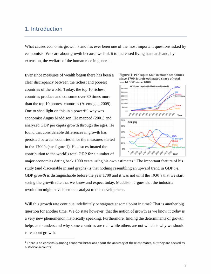
Econometrician Clive Granger introduced the concept of Granger causality in his 1969 paper. It

is a statistical hypothesis test that helps to determine the direction of causality between two

correlated variables. Granger argued that causality

could be tested for by using prior values of one

time series to predict later values of another time

series (see figure 2). The variable 𝑋 is said to

Granger-cause the variable 𝑌 if a time series of

𝑋 can be used to statistically significantly

predict a time series of 𝑌 taking into account 𝑌’s

correlation with its own past values (serial correlation).

This is done using a series of T-tests and F-tests. The null hypothesis is non-causality i.e. that 𝑋

does not Granger-cause 𝑌. The terms Granger causality tests and Granger non-causality tests will

be used interchangeably in this paper.

The idea of Granger-causality works in the sense that since our understanding of cause-effect

relationships often begins with us imagining that the cause happens before the effect. However,

this is where similarities between true causality and Granger-causality end. That one thing

consistently happens prior to another does not mean that the latter is caused by the former (the

post hoc ergo propter hoc fallacy). That being said, the concept of true causality is in itself

highly philosophical and problematic to define. Notwithstanding, the measure of how

consistently one variable is followed by another in combination with logical deduction (in our

case economic theory) is likely the closest we will come to true causality.

2.3. Literature Review

Several papers have concluded, in contradiction to neoclassical models that growth causes

savings. Edwards (1995) analyzed panel data from 36 Asian and Latin American countries in the

period 1970-1992. Using instrumental variables regression on lagged variables including gross

national product (GDP) growth, gross national savings (GDS) growth, population growth among

others, he found that output growth rate was one of the most impactful determinants of savings.

Similar results were found in Deaton & Paxson (1994). In an extensive 1993 study, Bosworth

Figure 2: Granger Causality

11

collected available evidence at the time and concluded that the growth to savings causality was

more robust than the savings to growth causality.

There is an equally large pool of research finding evidence for a growth-savings causality i.e. in

support of neoclassical theory. As shown by Houthakker (1961, 1965) and Modigliani (1970,

1990), some empirical evidence existed prior to the 1960’s in support of growth-savings

causation. This evidence though, is based on OLS regression without considerations about the

autoregressive properties or stationarity of the processes. Indeed, the problems of spurious

regressions and orders of integration were not yet developed and practiced prior to the 1960’s.

Some later papers also concluded savings-growth causality. Bacha (1990), Otani & Villanueva

1990, Stern (1991) and De Gregorio (1992) all conclude a saving to growth causation using OLS

on macro data from variety of countries. However, these results may exhibit some of the

problems explained in Toda & Yamamoto (1995) with possible pretesting bias and spurious

regressions due to insufficient knowledge about the order of integration of the series being

investigated.

Carroll & Weil (1994) used Granger causality tests on two different data sets; one of the OECD

countries and one of 64 randomly chosen countries. This is one of the few studies that uses a

large sample of countries. They find that growth Granger-causes savings, but not the converse.

They use Granger non-causality testing on VAR models in levels and in first difference, but do

not consider possible disturbances due to integration or cointegration. Carroll & Weil (2000)

continued their work and argued that a neoclassical growth model can support a growth to

savings causation if we consider consumer utility to depend on a “habit stock determined by past

consumption”.

Most of the research done after the 1990’s criticize the sampling and econometric methods (such

as OLS regressions and Granger causality tests) used in earlier research. New methodologies

applied on data from developing countries became popular.

Anorou & Ahmad (2001) tests for Granger-causality in 7 African countries. They base their

analysis on Dickey-Fuller unit root tests, Johansen cointegrations tests and VECMs. They find

that growth granger-causes savings in referred countries. Again, this method might suffer from

pretesting bias due to the causality testing being conditional on unit root and cointegration test

results. As previously mentioned, Johansen cointegration tests are sensitive to nuisance

12

parameters in sample sizes common in economic studies (Reimers 1992, Toda & Yamamoto

1995).

Odhiambo (2009) investigates the savings-growth nexus using household data from South

Africa. One limitation to Granger causality tests is that they are only reliablefor sets of two

variables. Odhiambo argues that a tri-variate model is called for and constructs such a model to

include real per capita income, GDS and foreign capital inflow. An ambitious tri-variate

causality test is followed and the researcher’s results are inconclusive.

Oladipo (2010) uses the Toda-Yamamoto procedure on microdata representing household

savings in Nigeria 1970-2006. The author finds unidirectional causality from GDP to GDS and

that the two series are cointegrated.

Sothan (2014) used data on per capita GDP and GDS gathered from Cambodia 1989-2012.

Granger causality tests in first difference was done as well as a Johansen cointegration test. The

author concludes no causation or cointegration and states that these variables are independent of

each other in Cambodia. The paper suffers from the same problems with possible pretesting bias

as Anorou & Ahmad (2001), Carroll & Weil (1994, 2000) among others.

Similarly to this thesis, Mohan (2006) examines the savings-growth causality nexus between

countries of different income levels. The four World Bank income categorizations are used and

the sample consists of 25 randomly selected countries (5 for each category except high income

which included 10 for some reason). Granger tests were done in levels for series found to be

stationary and in first difference for series found to be integrated of order one 𝑖(1). For

cointegrated series, a VECM was used. The author finds that in general, growth Granger-causes

savings and that causation differs depending on income level. For low income countries, the

causal direction was varied. For lower middle income countries, growth Granger-causes savings

but the converse was not found. For middle income economies, causality is bi-directional. In

high income countries, growth Granger-causes savings. In accordance with other aforementioned

research, this methodology allows for possible pretesting bias. Furthermore, the results lack in

generality due to a small sample of countries.

Evidently, some of the later studies have added a cointegration analysis to their methodology.

The concepts of Granger-causality and cointegration are closely related. Cointegration means, in

economic terms, that two time series exhibit a similar pattern and move together in long-run

13

equilibrium. Cointegration can at times be apparent simply by looking at a graph of the variables

of interest. However, tests must be carried out to determine the stochastic properties of the series.

Concerning growth and savings, both theory and empirical evidence suggest a positive

relationship between these two variables. Regardless of the causality direction, if one of these

variables increases or decreases, we expect the other to do the same i.e. we have reason to

believe that these variables are cointegrated. A (truly) cointegrated series implies Granger-

causality simply because Granger tests will yield significant results in such a situation. So if for

example two series are found to Granger-cause each other (in one direction or both directions),

but a cointegration test indicate no cointegration, we have contradictory results. This is the

reason why some studies have added a cointegration analysis as a cross-check to their causality

results. It is debatable whether a cointegration analysis legitimately strengthens causality

analyses due to the aforementioned problems with such tests. We cannot know with certainty if

cointegration results were produced under pretesting bias or not. A conflicting result between

cointegration tests and Granger causality tests does therefore not necessarily give us a reason to

suspect methodological error. Much of the allure with the Toda-Yamamoto method is to mitigate

pretesting bias, therefore such cointegration tests are excluded in this thesis. Hence, results in

this paper will only exhibit short run causality and no long run analysis.

3. Data

Data was collected from the World Bank World Development Indicators. The variables gathered

are gross national product per capita and gross domestic savings per capita in 2016 US$. Both

variables are log transformed in order to linearize their trends and narrow the differences

between them in absolute values. The dataset consists of four aggregated groups of countries

according to income level; low income, lower middle income, middle income and high income.

These groups are the average income of all countries within that income category. It is on these

averages that tests are done in the method section. Among the groups is represented every

country in the world. The definition of these income groups is done by the World Bank in their

14

2017 statement on classifications of these income groups.9 The classification is done based on

thresholds in gross national income (GNI) per capita. The thresholds are in 2017 US$:

Low Income: 𝐺𝑁𝐼/𝐶𝑎𝑝𝑖𝑡𝑎 < 1000.5

Lower Middle Income: 1000.5 < 𝐺𝑁𝐼/𝑐𝑎𝑝𝑖𝑡𝑎 ≤ 3995

Middle Income: 3995 < 𝐺𝑁𝐼/𝐶𝑎𝑝𝑖𝑡𝑎 ≤ 12 235

High Income: 𝐺𝑁𝐼/𝐶𝑎𝑝𝑖𝑡𝑎 > 12 235

This classification is updated annually due to changes in population, GDP growth, and exchange

rates etc. Inflation is accounted for. Naturally, it is possible to any grouping according to GDI

using any thresholds, but these four groups are well established and used in developmental

studies. Hence, for the sake of convenience, they will be used in this thesis. Some important

things to note concerning these income groups are:

1. Some countries wander between different income groups over time.

2. Aggregating data in this way creates a weighted average across many different countries

with different characteristics. There is no guarantee that this average is representative for

any one country.

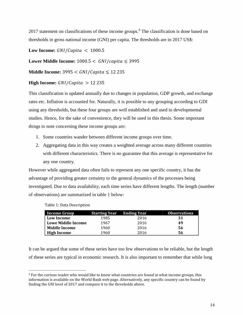
However while aggregated data often fails to represent any one specific country, it has the

advantage of providing greater certainty to the general dynamics of the processes being

investigated. Due to data availability, each time series have different lengths. The length (number

of observations) are summarized in table 1 below:

Table 1: Data Description

Income Group Starting Year Ending Year Observations Low Income 1985 2016 𝟑𝟏 Lowe Middle Income 1967 2016 49 Middle Income 1960 2016 56 High Income 1960 2016 56

It can be argued that some of these series have too few observations to be reliable, but the length

of these series are typical in economic research. It is also important to remember that while long

9 For the curious reader who would like to know what countries are found in what income groups, this information is available on the World Bank web page. Alternatively, any specific country can be found by finding the GNI level of 2017 and compare it to the thresholds above.

15

time series provide more observations, they are not by definition better than a shorter time series

because the fundamental processes creating the data might also change over time causing the

first few data points of the time series to not correspond with the last few, distorting inference.

One way to circumvent this problem is to use monthly or quarterly data to increase observations.

However, GDP and GDS reports are published annually, meaning quarterly or monthly data are

not readily available. It is possible to “transform” annual to quarterly or monthly data, but this

does not truly resolve the problem since the quarterly or monthly data points would be weighted

averages (guesses) of the annual data i.e. they would not de facto provide more data points or

explanatory power.

4. Method

In this section is presented the steps of the Toda-Yamamoto (TY) procedure followed by a

description of Dickey-Fuller unit root tests. The TY- method does necessitate the use of unit root

pretesting, but is not conditional on their results in the same way that VAR- of VECM based

Granger tests are. The function of unit root tests in the TY procedure is merely to find the

maximum order of integration that is suspected to be present in the process. For example, if the

unit root test statistic is very close to the critical value of the process being 𝑖(1), but does not

quite exceed it, or if for any other reason we are having trouble declaring a series 𝑖(0) or 𝑖(1),

the maximum order of integration that we suspect might be present in the process is 𝑖(1). That is,

in the presence of uncertainty, the higher order is assumed. Higher suspected orders if integration

makes the methodology less efficient, but not less consistent and unbiased (Toda & Yamamoto,

1995). All lags in this thesis are selected through a standard lag selection procedure where we

use an array of different criteria and choose the lag that is indicated by most of them (they will

often indicate the same lag).10

4.1. Method: The Toda Yamamoto Procedure

In their 1995 paper “Statistical Inference in Vector Autoregressions with Possibly Integrated

processes”, Hiro Toda and Taku Yamamoto present a method by which it is possible to set up a

VAR-model in levels (rather than in first-difference) and test restrictions on parameters “even if

10 In our case, the different criteria used are the Akaike Information Criterion (AIC), the Schwarz Bayesian Information Criterion (SBIC), and the Hannah and Quinn Information Critereon (HQIC).

16

the processes may be integrated or cointegrated of and arbitrary order”. They show that after

establishing a lag length 𝑝 through a regular lag selection criterion, they formulate a 𝑝 + 𝑚′ lags

VAR model where 𝑚’ is the maximum order of integration that is suspected to be present in the

process. The last 𝑚’ coefficients of the resulting model are then ignored and it is then possible to

test restrictions on the first 𝑝 coefficients of the model according to standard asymptotic theory.

Regarding Granger causality tests, Toda and Yamamoto stresses that the F-statistic usually

utilized in those tests is not normally distributed if the series tested are integrated or cointegrated.

They suggest using the modified Wald statistic (MWALD). This statistic is not normally

distributed either, but is more robust to said problems than a usual F-statistic (Toda & Yamamoto

1995). Furthermore, as is stressed throughout this thesis, many papers have used methodology

that allows for possible bias due to pretesting results. Available unit root hypothesis tests have

low power against the alternative in finite sample sizes creating a real risk of wrongly identifying

the order of integration, and cointegration tests are not suitable for typical economic time series

sample sizes due to nuisance parameter sensitivity. As explained above, the TY procedure takes

precautions against these problems by increasing lag order according to the highest suspected

order of integration. Additionally, since the causality test in the TY-method is done in the levels

of a VAR model, the standard asymptotic theory is valid when causality inference is done.

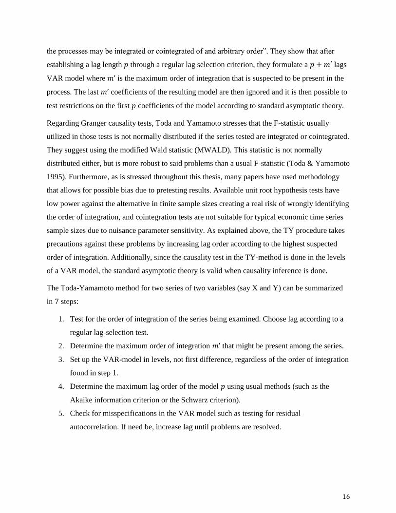
The Toda-Yamamoto method for two series of two variables (say X and Y) can be summarized

in 7 steps:

1. Test for the order of integration of the series being examined. Choose lag according to a

regular lag-selection test.

2. Determine the maximum order of integration 𝑚’ that might be present among the series.

3. Set up the VAR-model in levels, not first difference, regardless of the order of integration

found in step 1.

4. Determine the maximum lag order of the model 𝑝 using usual methods (such as the

Akaike information criterion or the Schwarz criterion).

5. Check for misspecifications in the VAR model such as testing for residual

autocorrelation. If need be, increase lag until problems are resolved.

17

6. Take the chosen VAR model and add 𝑚’ additional lags to each variable in each

equation. Ignore the coefficients of the last 𝑚’ lags (they are only there to ensure

asymptotics)

7. Test for Granger-causality using a standard Wald-test to test the null hypothesis that first

𝑝 coefficients of X the Y-equation is 0 and vice versa for the X-equation. The null

hypothesis is rejected for any p-value under 0.05 (or whatever critical value is selected).

These steps are followed a total of four times; once for each income group.

4.2. Method: the Dickey-Fuller Unit Root Test

The original Dickey-Fuller test was developed by David Dickey and Wayne Fuller in their

seminal 1979 paper. The test is executed as follows: We have an autoregressive process:

𝑋(𝑡) = 𝑎 + 𝑝𝑋(𝑡 − 1) + 휀𝑡 (10)

Where X is the variable of interest, 𝑎 is a constant, 𝑡 is a time index, 𝑝 is a coefficient and 휀 an

error term. If 𝑎 = 0 we have a random walk and if 𝑎 ≠ 0 we have a random walk with drift. For

this test however, it does not matter what type of random walk the process contains. The

parameter that matters here is 𝑝 on which we would like to test the following hypotheses:

H0: 𝑝 = 1

Against the alternative:

HA: 𝑝 < 1 (Absolute terms)

As mentioned earlier in the thesis, these tests have low power against the alternative hypothesis.

The problem arises due to how the null hypothesis is formulated. For finite sample sizes, these

tests have difficulty in distinguishing between true unit root processes where 𝑝 = 1 and near-unit

root processes where 𝑝 is close to 1, but not quite equal to 1. This creates a bias in the test

making it more likely to accept the null hypothesis in cases where 𝑝 is near 1 i.e. there is an

inherent risk of making a type-1 error. This problem is mitigated if the sample size is very large

as to add enough observations for the tests to be able to reliably make this distinction.

Conversely, however, the problem is amplified in the case of small samples sizes such as the

18

sample sizes of typical economic time series.11 Because of this, it can be argued there is value in

taking precautions against this inherent risk of unit root tests to wrongly identify the order of

integration of a series. This is what the Toda-Yamamoto procedure attempts to do by formulating

a methodology whose next step after unit root testing is not heavily determined by the results of

the unit root tests i.e. the next step will be the same whether or not the order of integration was

correctly identified.

Let us continue exploring the hypotheses of the ADF-tests listed above. If 𝑝 = 1, then 𝑋 depends

on its own previous values and on the error term, creating a situation where the mean changes

over time i.e. a non-stationary process. The trouble is that we cannot estimate the value of 𝑝

using a t-test because under the null hypothesis, not only 𝑋(𝑡) is non-stationary, but 𝑋(𝑡 − 1) is

in itself also non-stationary. Non-stationary processes do not become asymptotically normal

given large sample sizes (in accordance with the central limit theorem) and therefore the t-test

will not yield reliable results. One solution to this problem is to transform the above equation

into terms of the change in 𝑋(𝑡) i.e. a first difference transformation:

𝑋(𝑡) − 𝑋(𝑡 − 1) = 𝑎 + ((𝑝 − 1)𝑋(𝑡 − 1)) + 휀(𝑡) (11)

→ 𝛥𝑋 = 𝑎 + 𝛿(𝑥(𝑡 − 1)) + 휀 (12)

Where 𝛿 = 𝑝 − 1. In equation (12), if the null hypothesis 𝑝 = 1 is true, we see that the 𝛿 term

on the right-hand side becomes 0 and we are left with the expression: 𝛥𝑋 = 𝑎 + 휀 in which 𝛥𝑋

is stationary. However, if the null hypothesis is true, 𝑋(𝑡 − 1) is non-stationary, so when we

estimate 𝛿 using a t-statistic and compare it to a t-table we run into more problems. Since the

central limit theorem, once again, does not make non-stationary processes asymptotically

normal, there is nothing saying that the distribution the least squares estimator for 𝛿 is normal or

t-distributed, even for large sample sizes. In fact it follows a distribution of its own which was

tabulated by Dickey and Fuller in their 1979 paper. So we construct a t-statistic for 𝛿 and

compare it to some chosen critical value from the Dickey-Fuller distribution and we reject the

null hypothesis if the statistic is smaller than this critical value: 𝑡 < 𝐷𝐹.

11 These problems persist in all versions of the Dickey-Fuller test.

19

The “augmented” version of the Dickey-Fuller test is augmented in the sense that it is applicable

to more complicated processes, such as AR(2) or AR(3) processes,12 by adding a lag term to the

underlying regression equation:

𝛥𝑋(𝑡) = 𝑎 + 𝛿𝑋(𝑡 − 1) + ∑ 𝛽𝛥𝑋(𝑡 − 𝑖)

ℎ

𝑖=1

(13)

Where 𝛽 is the lag order of 𝛥𝑋 and ℎ is some finite number. This augmented version of the test

works for any lag order and is the more widely used version of the test and is the version that

will be utilized in this thesis. The alternative hypothesis of the test utilized in this thesis is trend-

stationarity.

A trend term (deterministic), or a drift term can be added to the augmented Dickey-Fuller unit

root test creating three versions of the test. All versions will be utilized in this thesis. For any

situation where uncertainty arises regarding the results of the unit root tests, we will be biased

towards choosing the higher order of integration since it is suspected i.e. it may or may not be

present in the process.

These two measures are taken to hedge against wrongly identifying the maximum order of

integration. When called for, we utilize graphs of the series to aid our analysis. The different

versions have different test statistics and critical values. The test including a trend term is least

likely to reject the null hypothesis since its test statistic is generally higher.

All lags for the Augmented Dickey-Fuller tests are selected through the standard lag-selection

routine. The benchmark significance level used in this thesis is 5 %, but since we are making

decisions about VAR model lags in accordance to how many integrating orders we suspect might

be present amongst the series, we will not simply accept or reject the null hypothesis according

to the 5 % level critical value all the time. As discussed above, in cases of uncertainty (for

example when the t-statistic is very close to a 5 % critical value) we will use graphs and

reasoning to decide the next step.

12 Rather than only AR(1) processes which is assumed in the original Dickey-Fuller test.

20

Figur 4

5. Results

In this section is presented the results yielded by the steps of the TY method discussed in the

method section. For the sake of simplicity, results are presented one income group at a time.

Subsequently follows a segment that briefly summarizes and compares the results of the different

series. Each income group analysis is initiated with a graphing of the two variables of interest. In

the unit root testing part, whenever the null hypothesis of non-stationarity is in any of the three

tests is accepted, additional graphing of the variables in first (or second) difference is done to

support our analysis.

5.1. Results: Low Income Countries

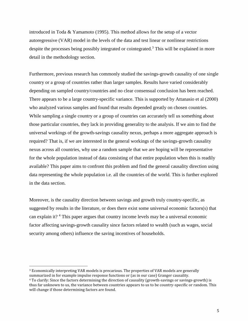
This series spans from 1985 to 2016 which mean that it consists of 31 observations. Our starting

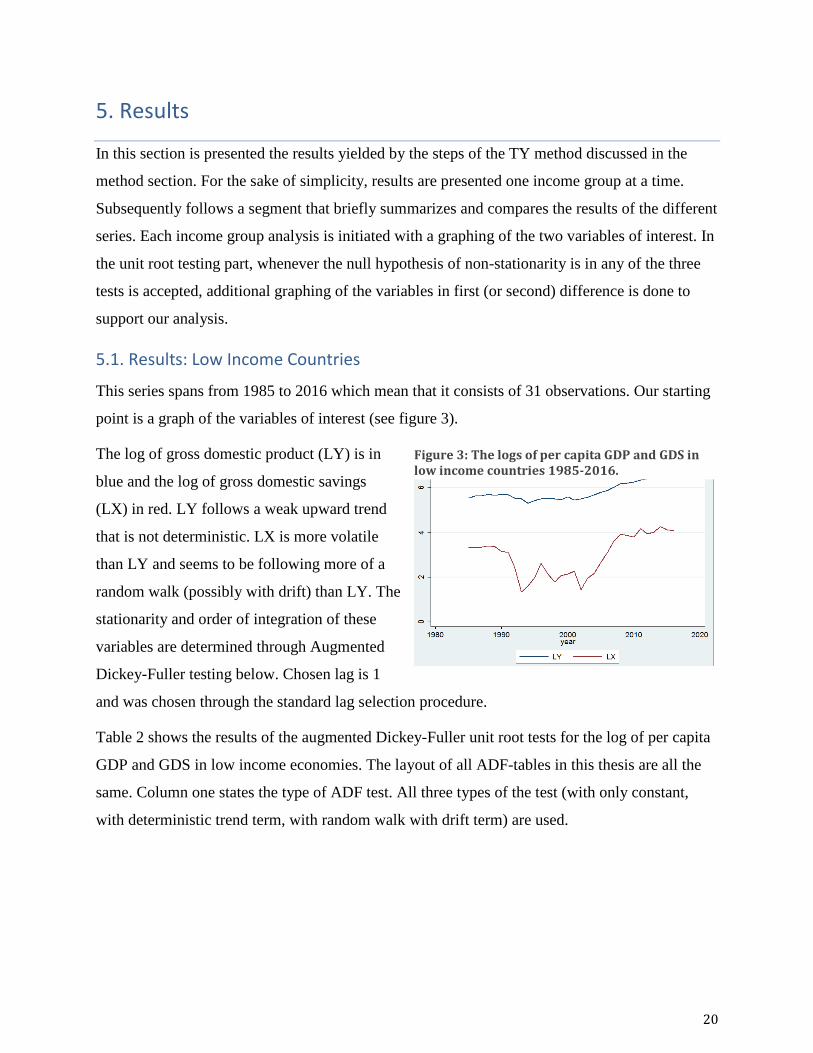
point is a graph of the variables of interest (see figure 3).

The log of gross domestic product (LY) is in

blue and the log of gross domestic savings

(LX) in red. LY follows a weak upward trend

that is not deterministic. LX is more volatile

than LY and seems to be following more of a

random walk (possibly with drift) than LY. The

stationarity and order of integration of these

variables are determined through Augmented

Dickey-Fuller testing below. Chosen lag is 1

and was chosen through the standard lag selection procedure.

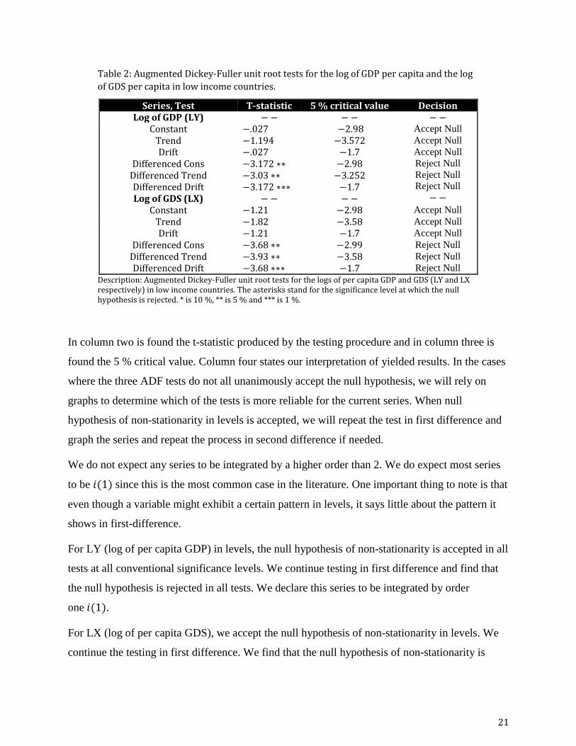
Table 2 shows the results of the augmented Dickey-Fuller unit root tests for the log of per capita

GDP and GDS in low income economies. The layout of all ADF-tables in this thesis are all the

same. Column one states the type of ADF test. All three types of the test (with only constant,

with deterministic trend term, with random walk with drift term) are used.

Figure 3: The logs of per capita GDP and GDS in low income countries 1985-2016.

21

Table 2: Augmented Dickey-Fuller unit root tests for the log of GDP per capita and the log

of GDS per capita in low income countries.

Series, Test T-statistic 5 % critical value Decision Log of GDP (LY) − − − − − −

Constant −.027 −2.98 Accept Null

Trend −1.194 −3.572 Accept Null

Drift Differenced Cons

Differenced Trend Differenced Drift Log of GDS (LX)

−.027 −3.172 ∗∗ −3.03 ∗∗ −3.172 ∗∗∗

− −

−1.7 −2.98

−3.252 −1.7 − −

Accept Null

Reject Null

Reject Null

Reject Null

− −

Constant −1.21 −2.98 Accept Null


Drift −1.21 −1.7 Accept Null

Differenced Cons −3.68 ∗∗ −2.99 Reject Null

Differenced Trend −3.93 ∗∗ −3.58 Reject Null

Differenced Drift −3.68 ∗∗∗ −1.7 Reject Null

Description: Augmented Dickey-Fuller unit root tests for the logs of per capita GDP and GDS (LY and LX respectively) in low income countries. The asterisks stand for the significance level at which the null hypothesis is rejected. * is 10 %, ** is 5 % and *** is 1 %.

In column two is found the t-statistic produced by the testing procedure and in column three is

found the 5 % critical value. Column four states our interpretation of yielded results. In the cases

where the three ADF tests do not all unanimously accept the null hypothesis, we will rely on

graphs to determine which of the tests is more reliable for the current series. When null

hypothesis of non-stationarity in levels is accepted, we will repeat the test in first difference and

graph the series and repeat the process in second difference if needed.

We do not expect any series to be integrated by a higher order than 2. We do expect most series

to be 𝑖(1) since this is the most common case in the literature. One important thing to note is that

even though a variable might exhibit a certain pattern in levels, it says little about the pattern it

shows in first-difference.

For LY (log of per capita GDP) in levels, the null hypothesis of non-stationarity is accepted in all

tests at all conventional significance levels. We continue testing in first difference and find that

the null hypothesis is rejected in all tests. We declare this series to be integrated by order

one 𝑖(1).

For LX (log of per capita GDS), we accept the null hypothesis of non-stationarity in levels. We

continue the testing in first difference. We find that the null hypothesis of non-stationarity is

22

rejected on the 5 % significance level in all tests and on the 1 % level in the test including a drift

term. We declare this series to also be integrated by order one 𝑖(1).

This means that the maximum order of integration that we suspect might be present among both

series 𝑚’ is 1 so that 𝑚’ = 1.

The next step of the Toda-Yamamoto procedure is to set up a VAR model in the levels of the

data and determine the maximum lag length of the series 𝑝. We then add 𝑚’ = 1 lags to this

number and check for misspecifications before conducting the Granger causality tests. The

maximum lag length 𝑝 of the VAR-model is 4 and was determined through the standard lag

selection procedure mentioned in the method section. Now we set up our VAR model with 𝑝 +

𝑚’ = 5 lags and check for misspecifications using a Lagrange-multiplier test for residual

autocorrelation, see table 3 below. The null hypothesis is no autocorrelation among residuals and

the alternative hypothesis is that there is autocorrelation among residuals. We reject the null for

any p-value below 0.05.

Table 3: Lagrange-multiplier test for residual autocorrelation

Lag Chi-Square Degrees of Freedom P-Value Decision 1 5.3757 4 0.25 Accept Null

2 6,6739 4 0.154 Accept Null

We cannot reject the null hypothesis of no autocorrelation in the residuals on any conventional

significance level. We proceed with the causality testing under the assumption that the model is

correctly specified.

Table 4 below displays the results of the Granger non-causality testing. The first row tests the

following hypotheses:

H0: Lagged (5) values of LX does not cause LY.

Against the alternative that:

Ha: Lagged (5) values of LY causes LX.

The last row tests the corresponding hypotheses for LX. The same hypothesis (with different

lags) are tested in the following three causality tests.

23

Table 4: Granger non-causality tests for the logs of per capita GDP (LY) and per capita GDS

(LX) in low income countries.

Hypothesis Wald Statistic Degrees of Freedom P-value

LX causes LY 33.07 5 0.000 LY causes LX 59.82 5 0.000

We reject the null hypothesis of no causation on the 1 % significance level for both variables and

state that they Granger-cause each other. In other words, the causality nexus in low income

countries seems to be bidirectional. We repeat the Toda-Yamamoto procedure for lower middle

income countries.

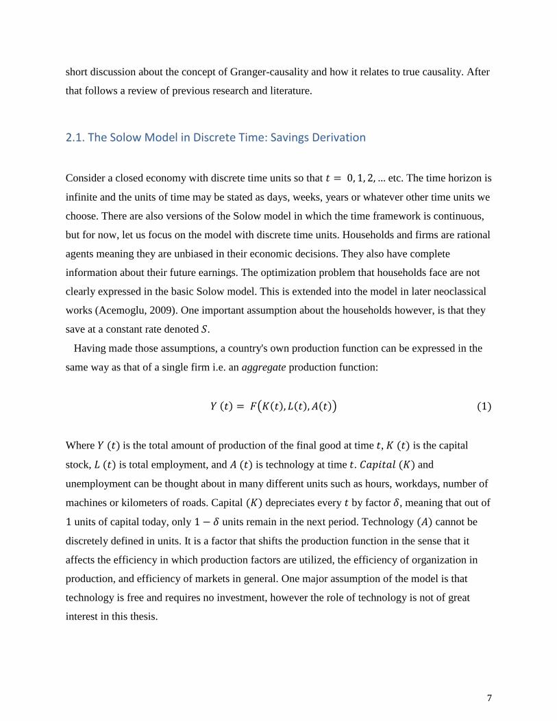
5.2. Results: Lower Middle Income Countries

This series spans from 1967 to 2016, making

49 observations. Once again we start by

graphing the two series:

LY in blue and LX in red. Both processes

exhibit an upward trend and a similar pattern

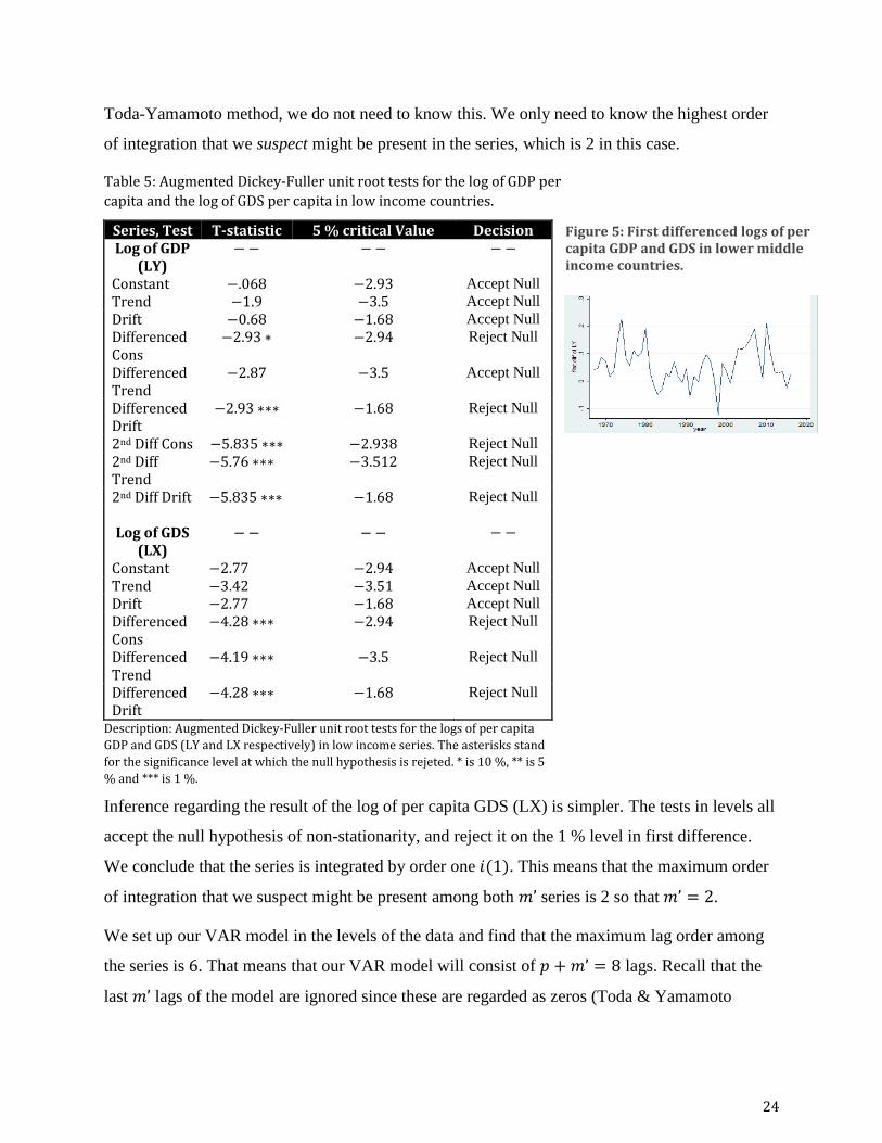
implying possible cointegration. Table 5 below

presents the results from the Augmented

Dickey-Fuller unit root tests. Chosen lag for is 2.

For LY in levels, the null hypothesis of non-stationarity cannot be rejected in any of the three

tests. In first difference, inference becomes a bit intricate. In the test with only a constant, the test

statistic is significant on the 10 % level and extremely close to being significant on the 5 % level.

Figure 5 depicts LY in first difference. No clear deterministic trend is discernable, but the mean

value could possibly revolve around 0 (indicating stationarity) or alternatively have a very slight

downward stochastic trend. We recall that the trend term test is unreliable when a trend is not

present and will yield biased results. We should therefore be suspicious of the results including a

trend term. With all of this taken in consideration, we argue that we do not have enough evidence

to confidently declare the order of integration of the series to be one 𝑖(1). At the very least, we

cannot comfortably say that we do not suspect higher orders of integration. We continue testing

in second difference and find that all tests reject the null hypothesis on the 1 % level. We

conclude that we are not certain if the series is 𝑖(1) or 𝑖(2). However, for the purposes of the

Figure 4: The logs of per capita GDP and GDS in lower middle income countries 1967-2016.

24

Toda-Yamamoto method, we do not need to know this. We only need to know the highest order

of integration that we suspect might be present in the series, which is 2 in this case.

Table 5: Augmented Dickey-Fuller unit root tests for the log of GDP per

capita and the log of GDS per capita in low income countries.

Series, Test T-statistic 5 % critical Value Decision Log of GDP

(LY) − − − − − −

Constant −.068 −2.93 Accept Null



Differenced Cons

−2.93 ∗ −2.94 Reject Null

Differenced Trend

−2.87 −3.5 Accept Null

Differenced Drift

−2.93 ∗∗∗ −1.68 Reject Null

2nd Diff Cons −5.835 ∗∗∗ −2.938 Reject Null

2nd Diff Trend

−5.76 ∗∗∗ −3.512 Reject Null

2nd Diff Drift −5.835 ∗∗∗ −1.68 Reject Null

Log of GDS

(LX)

− −

− −

− −

Constant −2.77 −2.94 Accept Null



Differenced Cons

−4.28 ∗∗∗ −2.94 Reject Null

Differenced Trend

−4.19 ∗∗∗ −3.5 Reject Null

Differenced Drift

−4.28 ∗∗∗ −1.68 Reject Null

Description: Augmented Dickey-Fuller unit root tests for the logs of per capita

GDP and GDS (LY and LX respectively) in low income series. The asterisks stand

for the significance level at which the null hypothesis is rejeted. * is 10 %, ** is 5

% and *** is 1 %.

Inference regarding the result of the log of per capita GDS (LX) is simpler. The tests in levels all

accept the null hypothesis of non-stationarity, and reject it on the 1 % level in first difference.

We conclude that the series is integrated by order one 𝑖(1). This means that the maximum order

of integration that we suspect might be present among both 𝑚’ series is 2 so that 𝑚’ = 2.

We set up our VAR model in the levels of the data and find that the maximum lag order among

the series is 6. That means that our VAR model will consist of 𝑝 + 𝑚’ = 8 lags. Recall that the

last 𝑚’ lags of the model are ignored since these are regarded as zeros (Toda & Yamamoto

Figure 5: First differenced logs of per capita GDP and GDS in lower middle income countries.

25

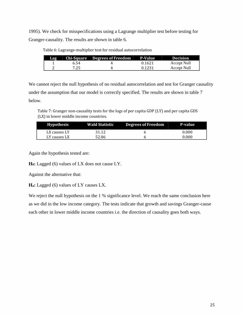
1995). We check for misspecifications using a Lagrange multiplier test before testing for

Granger-causality. The results are shown in table 6.



2 7.25 4 0.1231 Accept Null

We cannot reject the null hypothesis of no residual autocorrelation and test for Granger causality

under the assumption that our model is correctly specified. The results are shown in table 7

below.


(LX) in lower middle income countries.



Again the hypothesis tested are:

H0: Lagged (6) values of LX does not cause LY.

Against the alternative that:

Ha: Lagged (6) values of LY causes LX.

We reject the null hypothesis on the 1 % significance level. We reach the same conclusion here

as we did in the low income category. The tests indicate that growth and savings Granger-cause

each other in lower middle income countries i.e. the direction of causality goes both ways.

26

5.3. Results: Middle Income Countries

The data availability of the series for this income

group is better than for the previous income groups.

The series spans from 1960 to 2016 making 56

observations. The evolution of both variables

through time is presented in figure 6. Both series

move in a similar pattern implying cointegration.

The variance of LX seems to be greater than that of

LY, especially in the first two decades. The distance

between the two variables narrows with time i.e. the

series seems to be converging. The results of the ADF tests are presented in table 8 below. The

lag used is 2.

Table 8: Augmented Dickey-Fuller unit root tests for the log of GDP

per capita and the log of GDS per capita in low income countries.

Series, Test T-statistic 5 % critical value

Decision

Log of GDP (LY) − − − − − − Constant −0.55 −2.93 Accept Null



Differenced constant

−2.9 ∗ −2.93 Accept Null

Differenced Trend

−2.8 −3.5 Accept Null


2nd diff Cons −5.55 ∗∗∗ −2.93 Reject Null

2nd diff Trend −5.45 ∗∗∗ −3.5 Reject Null

2nd diff Drift −5.55 ∗∗∗ −1.68 Reject Null

Log of GDS (LX)

− −

− −

− − Constant −1.04 −2.93 Accept Null




−3.47 ∗∗∗ −2.93 Reject Null

Differenced Trend



Description: Augmented Dickey-Fuller unit root tests for the logs of per capita GDP

and GDS (LY and LX respectively) in low income series. The asterisks stand for the

significance level at which the null hypothesis is rejeted. * is 10 %, ** is 5 % and ***

is 1 %.

Figure7: The logs of per capita GDP and GDS in first difference 1960-2016.

Figure 6: The logs of GDP and GDS per capita 1960-2016 in middle income countries.

27

For the log of GDP per capita (LY) in levels (rows 1-3), all tests unanimously accept the null

hypothesis of non-stationarity. In first difference, the constant and trend tests both accept the null

hypothesis. We use a graph of the series (figure 7) to support our analysis. There is no

deterministic trend to speak of and there seems to be no clear stochastic trend. The series might

follow of a random walk that revolves around 0. However, we cannot reject the null hypothesis

of non-stationarity at the 5 % level in the test including only a constant. We cannot comfortably

say that the highest order of integration we suspect might be present in the process is 1 (𝑖(1)).

We execute the tests again in second difference (rows 7-9). The null hypothesis is rejected in all

tests and we argue that we cannot confidently say if the series is integrated by order 𝑖(1) or by

order 2 𝑖(2).

The tests in levels of LX (log of GDS per capita, rows 10-12) cannot reject the null hypothesis

on any conventional level. In first difference, the null is rejected on the 10 % level in all tests and

on the 1 % level in the test including only a constant and in the test including a drift term. The

graph displays no deterministic trend meaning that we should not expect the test including a

trend term to yield unbiased results in this case. We argue that the 1 % significance rejection of

the tests including a constant and a drift term together with our suspicion of the trend term test is

evidence enough to conclude that the series is integrated by order 1 𝑖(1). We also recall that even

if we are wrong and the series is in fact 𝑖(2) it will not change the numbers of our Toda-

Yamamoto method since we only need the highest number of integration that we suspect is

present among both series. We already suspect LY to be 𝑖(2).

Since we declared LX to be 𝑖(1) and we were unable to determine if LY is 𝑖(1) or 𝑖(2), the

maximum order of integration we suspect might be present among both series 𝑚’ is 2 so that

𝑚’ = 2. We set up our VAR model in levels and find through the usual lag selection procedure

that the maximum significant lag order in the model is 6. This means that the lag of our VAR

model is 𝑝 + 𝑚’ = 8. Before conducting the Granger non-causality tests, we once again check

for misspecification through a Lagrange Multiplier test, see table 9 below.



2 0.1845 4 0.996 Accept Null

28

The null hypothesis of no serial correlation at lag order cannot be rejected on any customary

significance level. Once again we proceed under the premise that the model is correctly

specified. The results of the Granger non-causality tests are presented below in table 10.





In the first row, we reject the null hypothesis that LX (log of per capita GDS) does not cause LY

(log of per capita GDP) on the 1 % level. In the second row, we cannot reject the null hypothesis

that LY does not cause LX on the 5 % level, but we reject it on the 10 % level. Nevertheless,

chosen significance level for our causality testing is 5 %. We conclude that in middle income

countries, savings Granger-causes growth, but the converse was not convincingly verified. We

carry on with our final Toda-Yamamoto routine in high income economies.

5.4. Results: High Income Countries

This series spans from 1970 to 2016 making 46 observations. The evolution of both variables

through time can be found in figure 8. The log of

GDP per capita (LY) in blue and the log of GDS

per capita (LX) in red. The series follow a similar

pattern through time. Neither seems to have a much

larger variance that the other and they both have a

clear upward, but declining trend. The distance

between the series increase slightly over time. The

ADF testing results are presented in table 11 below.

For LY in levels, both the constant test and the drift

test reject the null hypothesis if non-stationarity at the 5 % level, but the drift term test cannot

reject the null hypothesis on any conventional level, making inference difficult. Looking at the

graph of the variable in levels (figure 8) it is hard to discern by eye if the trend is closely

deterministic or if it is stochastic. It is therefore hard to know which test is most likely to be

Figure8: The logs of per capita GDP and GDS in high income countries 1970-2016.

29

unbiased. We continue testing in first difference. Both the trend term test and the drift term test

reject the null hypothesis on the 5% significance level, but the test including only a constant

cannot reject the null hypothesis. Figure 9 shows the series in first difference. The variable

exhibits a random walk with a clear declining trend, meaning we should trust the test with a drift

term the most and that the test including only a constant is likely to yield biased results in this

scenario. Hence we assess that there is no real reason to suspect any higher order of integration

than 1. That being said, we cannot say if the process is stationary in levels 𝑖(0) or if it is

integrated by order one 𝑖(1). LX shows a similar situation, but in first difference, the null is

unanimously rejected at the 1 % level in all tests i.e. we quite clearly find LX to be integrated by

order one 𝑖(1). We state that the highest order of integration that we suspect is present within

either series is 1 so that 𝑚’ = 1.

Table 4: Augmented Dickey-Fuller unit root tests for the log of GDP

per capita and the log of GDS per capita in high income countries.

Series, Test T-statistic 5 % critical value

Decision

Log of GDP (LY) − − − − − − Constant −3.34 ∗∗ −2.93 Reject Null


Drift −3.34 ∗∗∗ −1.68 Reject Null



Differenced Trend −3.87 ∗∗ −3.51 Reject Null


Log of GDS (LX)

− −

− −

− − Constant −2.78 −2.94 Accept Null


Drift −2.78 ∗∗∗ −1.68 Reject Null


−4.13 ∗∗∗ −2.95 Reject Null

Differenced Trend −4.9 ∗∗∗ −3.52 Reject Null


Description: Augmented Dickey-Fuller unit root tests for the logs of per capita GDP

and GDS (LY and LX respectively) in low income series. The asterisks stand for the

significance level at which the null hypothesis is rejeted. * is 10 %, ** is 5 % and ***

is 1 %.

We proceed by setting up our VAR model in the levels of the data and find through the usual lag

selection method that the maximum significant lag order in the model is 7. This means that the

Figure 9: The log of GDP per capita in first difference 1970-2016 in high income countries.

30

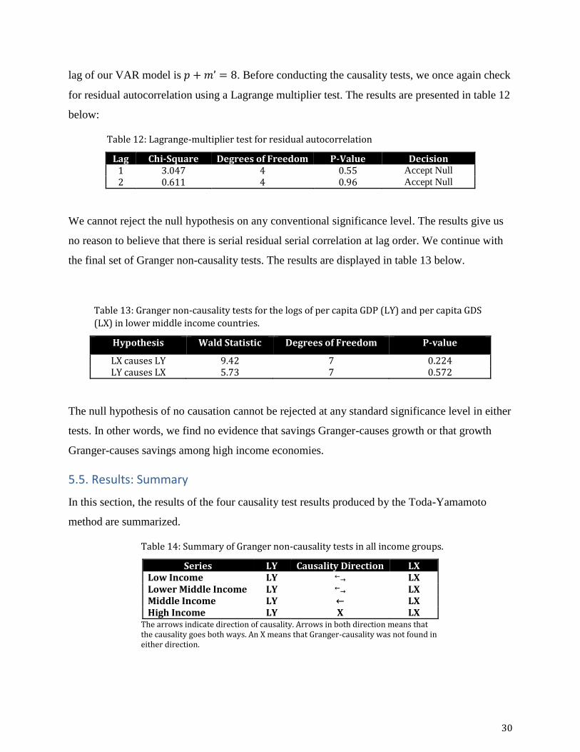
lag of our VAR model is 𝑝 + 𝑚’ = 8. Before conducting the causality tests, we once again check

for residual autocorrelation using a Lagrange multiplier test. The results are presented in table 12

below:



2 0.611 4 0.96 Accept Null

We cannot reject the null hypothesis on any conventional significance level. The results give us

no reason to believe that there is serial residual serial correlation at lag order. We continue with

the final set of Granger non-causality tests. The results are displayed in table 13 below.





The null hypothesis of no causation cannot be rejected at any standard significance level in either

tests. In other words, we find no evidence that savings Granger-causes growth or that growth

Granger-causes savings among high income economies.

5.5. Results: Summary

In this section, the results of the four causality test results produced by the Toda-Yamamoto

method are summarized.

Table 14: Summary of Granger non-causality tests in all income groups.

Series LY Causality Direction LX Low Income LY ←

→ LX Lower Middle Income LY ←→ LX Middle Income LY ← LX High Income LY X LX

The arrows indicate direction of causality. Arrows in both direction means that the causality goes both ways. An X means that Granger-causality was not found in either direction.

31

Table 14 contains a summary of the causality directions of the four income groups that were

found in the results section. For low and lower middle income economies, the direction of

causation between savings and growth is found to be bidirectional i.e. they Granger-cause each

other. For middle income economies, savings granger-causes growth at a 5 % significance level,

but the opposite was not found.13 For high income economies, no Granger-causality was found in

any direction for any conventional significance level.

6. Conclusion and Discussion

Here follows some concluding remarks about the empirical findings and a brief discussion about

them including answers to the research questions stated in the introduction.

While it is logical that savings should cause growth through its interaction with capital

accumulation, the opposite, that growth should cause savings, is just a reasonable i.e. how can

anyone save money if they had no income to begin with? This duality is reflected in our results

for low- and lower middle income economies where we find that growth and savings granger-

cause each other. These findings might partly explain the considerable variety among results of

previous research that uses only a single country. For middle income countries, we find that

savings granger-causes growth, but the opposite is not found 5 % significance level. We note

however, that growth was found to Granger-cause savings is this income group on the 10 %

level. For high income countries we find no Granger-causation in either direction between

savings and growth.

Let us recall this paper’s research questions:

1. What is the general causal relationship between growth and savings in the world?

For high income countries, no Granger-causation was found. However, since bidirectional

Granger-causality was found at the 5 % significance level in low and lower middle income

countries and at the 10 % level in middle income countries, our findings indicate that savings and

growth in the world generally (on average) Granger-cause each other, confirming and

contradicting both neoclassical theory and empirical findings.

13 Although, it was on the 10 % significance level.

32

2. Does the direction of causation vary with country income levels?

The answer to this question according to our findings is both yes and no. We found a

bidirectional causal relationship between savings and growth in each income category except the

high income group. In middle income countries, this relationship was only significant on the 10

% significance level. It seems to be more troublesome to determine the causal direction of

savings and growth in higher income countries than in lower income countries. The question

why is interesting and hard to answer without more information. Perhaps savings and growth are

more independent among wealthy countries because if households are wealthy enough, they have

the opportunity to save money regardless of their country’s growth rate i.e. savings in these

economies might be determined by other factors. These factors are a topic for further research.

Our findings are not in line with Mohan (2006) who concluded a general savings to growth

causation. Recall, however than those results were found using a small sample size. Our results

are not meaningfully in line with other previous studies either since these have primarily focused

on singular countries or groups of countries. Our findings showcase a need for new economic

growth models exploring the reasons why the savings-growth causality direction is less clear in

high income economies.

33

References

Acemoglu, D (2009), Introduction to Modern Economic Growth. Princeton University Press.

Anoruo, E & Ahmad, Y. 2001. Causal relationship between domestic savings and economic

growth: Evidence from seven African countries. African Development Review 13 (2): 238- 249.

Attanasio, Orazio P, Lucio Picci & Antonello E. Scorcu. 2000. Saving, Growth, and Investment:

A Macroeconomic Analysis using a Panel of Countries. Review of Economics and Statistics 82

(2): 182-211.

Bacha, E L. 1990. A three-gap model of foreign transfers and the GDP growth rate in developing

countries. Journal of Development Economics 32 (2): 279-296.

Bosworth, B P. 1993. Saving and Investment in Global Economy. Brookings, Washington DC.

Carroll, C. & Weil, D. 1994. Saving Behavior in Ten Developing Countries. Carnegie -

Rochester Conference Series on Public Policy. Vol. 40.

Carroll, C D, Overland, J & Weil, D N. 2000. Saving and growth with habit formation. American

Economic Review 90 (3): 341-355.

Deaton, A & Paxson, C. 1994. Saving, Growth and Aging in Taiwan. Studies in the Economics

of Aging: 331-362.

34

De Gregorio, J. 1992. Economic growth in Latin America. Journal of Developmental Economics

39 (1): 59-84.

Dickey, D & Fuller, W A. 1979. Distribution of the Estimators for Autoregressive Time Series

with a Unit Root. Journal of the American Statistical Association 74 (336): 427-431.

Edwards, S. 1995. Why are Saving Rates so Different Across Countries? : An International

Comparative Analysis. Journal of Developmental Economics 51 (1): 5-44.

Granger, Clive W J. 1969. Investigating Causal Relations by Econometric Models and Cross-

spectral Methods. Econometrica 37 (3): 424-438

Houthakker, H S. 1961. The present state of consumption theory. Econometrica 19 (4): 704-740.

Houthakker, H S. 1965. On some determinants of saving in developed and under-developed

countries. Problems in Economic Development: 212-227.

Johansen, S. and Juselius, K. 1990. Maximum Likelihood Estimation and Inference on

Cointegration — with Applications to the Demand for Money. Oxford Bulletin of Economics and

Statistics 52 (2): 169–210.

Maddison, A. 2001. The World Economy. Historical Statistics. OECD Publications Service.

Modigliani, F. 1970. The Life Cycle Hypothesis of Saving and Intercountry Difference in Saving

Ratio, in W.A. Eltis, M.F. Scott and J.N. Wolfe (eds.), Induction, Trade and Growth: Essays in

Honor of Sir Roy Harrod, Clarendon Press, London.

Modigliani, F. 1990. Recent Development in Saving Rates: A Life Cycle Perspective. Frisch

Lecture, Sixth World of Congress of the Econometric Society, Barcelona, Spain.

Odhiambo, N M. 2009. Savings and economic growth in South Africa: A multivariate causality

test. Journal of policy Modeling 31 (5): 708-718.

Oladipo, OS. Does Saving Really Matter for Growth In Developing Countries? The Case of a

Small Open Economy. International Business & Economics Research Journal 9(4): 87-94.

Otani, I & Villanueva, D. 1990. Long-term growth in developing countries and its determinants:

An empirical analysis. World Development 18 (6): 769-783.

35

Phillips, CB & Toda, H. 1993. Limit Theory in Cointegrated Vector Autoregressions.

Econometric Theory 9 (1): 150-153.

Reimers, HE. 1992. Comparisons of tests of multivariate cointegration. Statistical Papers 33 (1):

335-359.

Solow, Robert M. 1956. A contribution to the theory of economic growth. Quarterly Journal of

Economics 70 (1): 65-94

Sothan, S. 2014. Causal Relationship between Domestic Saving and Economic Growth:

Evidence from Cambodia. International Journal of Economics and Finance 6 (9).

Stern, N. (1991). Public policy and the economics of development. European Economic Review

35 (2): 241-271.

Toda, Hiro Y & Yamamoto, Taku. 1995. Statistical inference in vector autoregressions with

possibly integrated processes. Journal of Econometrics 66 (1-2): 225-250.

Documents

Does Saving Cause Growth?