Does Hedging Success Matter? An Empirical Study of Jet

University of South Florida University of South Florida

Scholar Commons Scholar Commons

Graduate Theses and Dissertations Graduate School

April 2020

Does Hedging Success Matter? An Empirical Study of Jet Fuel Does Hedging Success Matter? An Empirical Study of Jet Fuel

Hedging in the U.S. Airline Industry Hedging in the U.S. Airline Industry

Brian Hornung University of South Florida

Follow this and additional works at: https://scholarcommons.usf.edu/etd

Part of the Economics Commons

Scholar Commons Citation Scholar Commons Citation Hornung, Brian, "Does Hedging Success Matter? An Empirical Study of Jet Fuel Hedging in the U.S. Airline Industry" (2020). Graduate Theses and Dissertations. https://scholarcommons.usf.edu/etd/8225

This Dissertation is brought to you for free and open access by the Graduate School at Scholar Commons. It has been accepted for inclusion in Graduate Theses and Dissertations by an authorized administrator of Scholar Commons. For more information, please contact [email protected].

http://scholarcommons.usf.edu/

http://scholarcommons.usf.edu/

https://scholarcommons.usf.edu/

https://scholarcommons.usf.edu/etd

https://scholarcommons.usf.edu/grad

https://scholarcommons.usf.edu/etd?utm_source=scholarcommons.usf.edu%2Fetd%2F8225&utm_medium=PDF&utm_campaign=PDFCoverPages

http://network.bepress.com/hgg/discipline/340?utm_source=scholarcommons.usf.edu%2Fetd%2F8225&utm_medium=PDF&utm_campaign=PDFCoverPages

mailto:[email protected]

Does Hedging Success Matter? An Empirical Study of Jet Fuel Hedging

in the U.S. Airline Industry

by

Brian Hornung

A dissertation submitted in partial fulfillment

of requirements for the degree of

Doctor of Philosophy in Economics

Department of Economics

College of Arts and Sciences

University of South Florida

Co-Major Professor: Christopher Thomas, Ph.D.

Co-Major Professor: Bradley Kamp, Ph.D.

Andrei Barbos, Ph.D.

Diogo Baerlocher, Ph.D.

Tapas Das, Ph.D.

Date of Approval:

April 3, 2020

Keywords: risk management, firm value, buying market share, principal-agent problem

Copyright © 2020, Brian Hornung

i

TABLE OF CONTENTS

List of Tables ................................................................................................................................. iv

List of Figures ................................................................................................................................ vi

Abstract ......................................................................................................................................... vii

Chapter One: Introduction ...............................................................................................................1

1.1 Background on Jet Fuel Price Hedging .........................................................................1

1.2 An Economic Perspective of Hedging and Firm Value .................................................2

1.3 Contributions to the Literature .......................................................................................4

1.4 Organization ...................................................................................................................5

Chapter Two: Literature Review of Jet Fuel Hedging in the Airline Industry ..............................11

2.1 Introduction to the Hedging Literature ........................................................................11

2.1.1 Theoretical Hedging Literature Overview ....................................................11

2.1.2 Empirical Hedging Literature Overview ......................................................12

2.1.3 Jet Fuel Hedging Literature Overview ..........................................................13

2.2 Theoretical Literature: Hedging and Firm Value ........................................................14

2.3 Empirical Literature: Commodity, Foreign Currency, and Interest Rate

Hedging ........................................................................................................................16

2.4 Jet Fuel Price Hedging in the Airline Industry ............................................................18

2.5 Overview of Commodity Price Hedging .....................................................................23

Chapter Three: Data Sources and Collection .................................................................................25

3.1 Database Overview ......................................................................................................25

3.2 Compustat Database.....................................................................................................26

3.3 EDGAR Database ........................................................................................................27

3.3.1 Jet Fuel Hedging Measures from Form 10-K ...............................................27

3.3.1.1 Percentage of Next Year’s Jet Fuel Requirements Hedged ...........28

3.3.1.2 Gains and Losses from Jet Fuel Hedges ........................................29

3.3.2 Other Variables Taken from Form 10-K ......................................................31

3.4 Bureau of Transportation Statistics Databases ............................................................31

3.4.1 T-100 Data Bank ...........................................................................................32

3.4.2 DB1B Survey ................................................................................................34

Chapter Four: Hedging Gains and Losses and Firm Value ...........................................................39

4.1 Background ..................................................................................................................39

4.1.1 Justification for Replication ..........................................................................39

4.1.2 Study Extension: Hedging Gains and Losses ...............................................41

ii

4.2 Jet Fuel Price Exposure ................................................................................................43

4.3 Summary Statistics and Variable Discussion ..............................................................44

4.4 Determinants of Jet Fuel Hedging ...............................................................................47

4.4.1 Predicted Effects on Jet Fuel Hedging ..........................................................48

4.4.2 Estimated Effects on Jet Fuel Hedging .........................................................50

4.4.2.1 Dropping Statistically Weak Explanatory Variables .....................50

4.4.2.2 Final Estimates ...............................................................................52

4.4.3 Summary of Determinants of Jet Fuel Hedging ...........................................54

4.5 Effect of Jet Fuel Hedging on Firm Value ...................................................................55

4.5.1 Firm Value Models and Specifications .........................................................55

4.5.2 Size of the Hedging Premium .......................................................................56

4.5.3 Possible Endogeneity between Jet Fuel Hedging and Firm Value ...............58

4.5.4 Hedging Premium through Capital Expenditures .........................................59

4.5.4.1 Interaction of Capital Expenditures with Jet Fuel Hedging ...........60

4.5.4.2 Two-stage Regression of Hedging on Capital Expenditures

and Firm Value ....................................................................................62

4.5.5 Hedging Premium over Time........................................................................64

4.6 Jet Fuel Hedging Gains and Losses and Firm Value ...................................................65

4.6.1 Jet Fuel Hedging Realized Gains and Losses and Firm Value .....................66

4.6.2 Effect of Successful Jet Fuel Hedging on the Hedging Premium .................68

4.7 Conclusion ...................................................................................................................69

Chapter Five: Using Successful Jet Fuel Hedges to Increase Market Share .................................84

5.1 Investment Opportunities in the Airline Industry ........................................................84

5.1.1 Investment Project Classifications ................................................................85

5.1.2 Principal-agent Problems, Buying Market Share, and Hedging ...................86

5.2 Changes in Market Share and Jet Fuel Hedging Gains and Losses .............................88

5.2.1 Airline Selection, Realized Gains and Losses, and Time Frame ..................89

5.2.2 Market Definitions ........................................................................................90

5.2.3 Measuring Changes in Market Share ............................................................91

5.2.4 Model for Changes in Market Share and Hedging Gains and Losses ..........93

5.2.5 Restrictions on the Market Sample ...............................................................94

5.3 Analysis of Market Sample and Estimation Results for Southwest Airlines...............95

5.3.1 Market Sample and Sample Restrictions ......................................................96

5.3.2 Estimation Results ........................................................................................97

5.3.3 Robustness Checks: Airport Markets and Different Airline Model

Estimates ..........................................................................................................99

5.3.3.1 Estimates with Change in Market Definition ...............................100

5.3.3.2 Model Estimates for Other Airlines .............................................100

5.4 Conclusion .................................................................................................................101

Chapter Six: Hedging Literature Contributions and Future Research .........................................113

6.1 Summary of Dissertation Findings ............................................................................113

6.1.1 Contributions from Hedging Gains and Losses and Study

Reproduction ..................................................................................................113

6.1.2 Contributions to Principal-agent Problems, Antitrust Concerns, and

iii

Hedging ..........................................................................................................115

6.2 Future Research .........................................................................................................116

References ....................................................................................................................................118

iv

LIST OF TABLES

Table 1.1: Yearly Jet Fuel Expense as a Percent of Total Operating Expense .......................10

Table 3.1: Names and Locations of Variables within Compustat ...........................................36

Table 4.1: Summary Statistics Used in Replication Regressions ...........................................72

Table 4.2: Carter, Rogers, and Simkins (2006) Table V Expected Signs and Results ...........73

Table 4.3: Factors That Influence Jet Fuel Hedging by Airlines ............................................74

Table 4.4: Firm Value on Jet Fuel Hedging Regressions........................................................75

Table 4.5: Firm Value Regressions with First Differences .....................................................76

Table 4.6a: Interaction of Capital Expenditures-to-sales on Jet Fuel Hedging ........................77

Table 4.6b: Interaction of Capital Expenditures-to-sales (Lease Adjusted) on Jet Fuel

Hedging ..................................................................................................................78

Table 4.7: Two-stage Regression of Predicted Capital Expenditures on Firm Value ............79

Table 4.8: Effect of Jet Fuel Hedging on Firm Value by Year ...............................................80

Table 4.9a: Firm Value on Jet Fuel Hedging Gains and Losses Regressions ...........................81

Table 4.9b: Firm Value on Jet Fuel Hedging Gains and Losses Regressions (Excluding

Outliers) .................................................................................................................82

Table 4.10: Firm Value Regressions with Interaction of Jet Fuel Hedging and

Successful Hedging ................................................................................................83

Table 5.1: Restrictions on Market Sample Size for Southwest Airlines ...............................104

Table 5.2: Average Change in Market Share for Each Sample Restriction for

SouthwestAirlines ................................................................................................105

Table 5.3: Southwest Airlines Jet Fuel Hedging on Market Share (Measures 1 and 2) .......106

Table 5.4: Southwest Airlines Jet Fuel Hedging on Market Share (Measure 3)...................107

v

Table 5.5: Southwest Airlines Jet Fuel Hedging on Market Share (Measure 4)...................108

Table 5.6: Southwest Airlines Jet Fuel Hedging Indicator on Airport Market Share

(Measure 4) ..........................................................................................................109

Table 5.7: American Airlines Jet Fuel Hedging on Market Share (Measure 4) ...................110

Table 5.8: Alaska Airlines Jet Fuel Hedging on Market Share (Measure 4) ........................111

Table 5.9: JetBlue Airways Jet Fuel Hedging on Market Share (Measure 4).......................112

vi

LIST OF FIGURES

Figure 1.1: Spot Prices for US Gulf Coast Jet Fuel and WTI Crude Oil ...................................9

Figure 3.1: Alaska Airlines Expected Jet Fuel Requirements Hedged from 2008 10-K

Statement................................................................................................................37

Figure 3.2: United Airlines Jet Fuel Hedging Gains and Losses from 2014 10-K

Statement................................................................................................................38

Figure 4.1: Box Plot of Realized Gains and Losses (Millions) from Jet Fuel Hedging

(Non-zero Values) ..................................................................................................71

Figure 5.1: Realized Gains and Losses (Millions) from Jet Fuel Hedging for Sample

Airlines .................................................................................................................104

vii

ABSTRACT

Airlines commonly employ hedging as a risk management strategy to protect themselves

against sudden, unpredictable increases in the price of jet fuel. In a seminal paper by Carter,

Rogers, and Simkins (2006), it is established that jet fuel hedging by airlines increases the firm

value of the airline. This dissertation replicates their study using an expanded dataset over a

greater period of time. This study finds a smaller “hedging premium” than Carter, Rogers, and

Simkins (2006). It is shown that the leasing of aircraft plays an important role in the relationship

between the hedging premium and capital expenditures.

The measure of jet fuel hedging used in the previous studies, the percentage of next

year’s fuel requirements hedged, accounts for the amount of hedging done by the airline, but it

does not consider the performance of the jet fuel hedges. This dissertation for the first time

determines the effect of jet fuel hedging performance, as measured by the realized gains and

losses from jet fuel hedging, on the value of the firm. The analyses find that the realized gains

and losses have a negative relationship with firm value. However, after identifying outliers (such

as the significant hedging losses in 2009 resulting from falling jet fuel prices during the financial

crisis) using a simple box plot and removing them from the sample, realized gains and losses

show a positive correlation with firm value.

Furthermore, successful hedging may induce principal-agent issues such as buying

market share behavior. When an airline experiences a run of hedging success, a manager may

mistakenly believe that the cost of jet fuel is decreasing. This is not the case, however, as the

viii

cost of using jet fuel is the price that can be received selling it on the open market, not the price

paid for the jet fuel. A manager may attempt to pass on the “savings” to consumers in the form

of lower fares, lowering the price below its profit-maximizing level. This in turn can increase

the airline’s market share, although it comes at the expense of reduced profit. This dissertation

tests the relationship between successful jet fuel hedging and market share. A positive and

statistically significant correlation between successful hedging and market share is found for

Southwest Airlines and American Airlines, two carriers known for successful hedging, but

statistically insignificant results for smaller carriers Alaska Airlines and JetBlue Airways.

1

CHAPTER ONE:

INTRODUCTION

1.1 Background on Jet Fuel Price Hedging

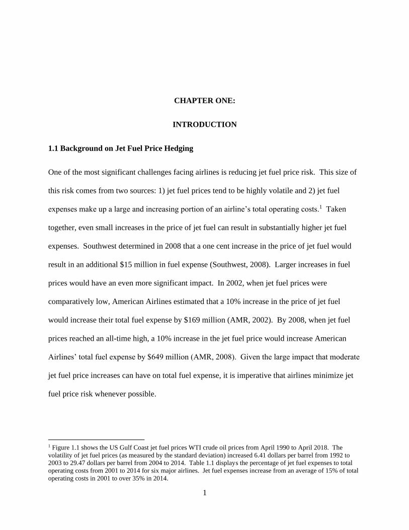
One of the most significant challenges facing airlines is reducing jet fuel price risk. This size of

this risk comes from two sources: 1) jet fuel prices tend to be highly volatile and 2) jet fuel

expenses make up a large and increasing portion of an airline’s total operating costs.1 Taken

together, even small increases in the price of jet fuel can result in substantially higher jet fuel

expenses. Southwest determined in 2008 that a one cent increase in the price of jet fuel would

result in an additional $15 million in fuel expense (Southwest, 2008). Larger increases in fuel

prices would have an even more significant impact. In 2002, when jet fuel prices were

comparatively low, American Airlines estimated that a 10% increase in the price of jet fuel

would increase their total fuel expense by $169 million (AMR, 2002). By 2008, when jet fuel

prices reached an all-time high, a 10% increase in the jet fuel price would increase American

Airlines’ total fuel expense by $649 million (AMR, 2008). Given the large impact that moderate

jet fuel price increases can have on total fuel expense, it is imperative that airlines minimize jet

fuel price risk whenever possible.

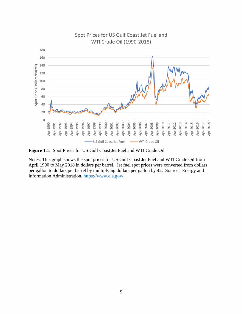
1 Figure 1.1 shows the US Gulf Coast jet fuel prices WTI crude oil prices from April 1990 to April 2018. The

volatility of jet fuel prices (as measured by the standard deviation) increased 6.41 dollars per barrel from 1992 to

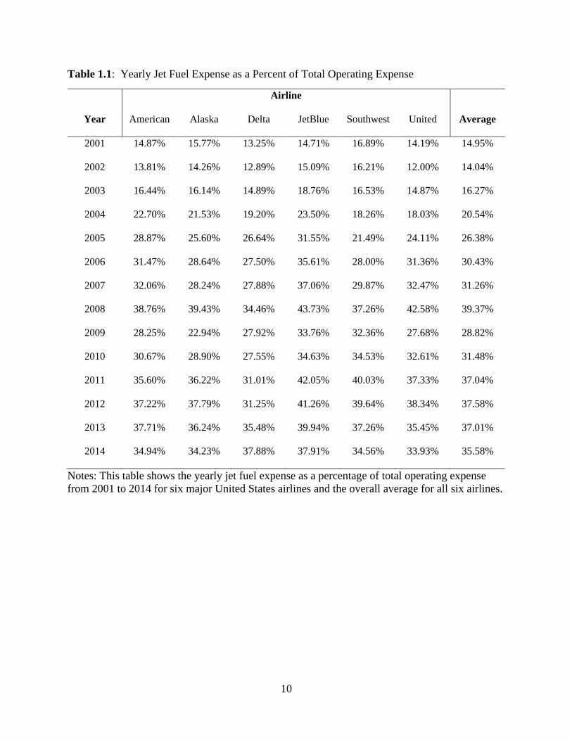
2003 to 29.47 dollars per barrel from 2004 to 2014. Table 1.1 displays the percentage of jet fuel expenses to total

operating costs from 2001 to 2014 for six major airlines. Jet fuel expenses increase from an average of 15% of total

operating costs in 2001 to over 35% in 2014.

2

The most common risk management activity airlines use to decrease jet fuel price risk is

through hedging. Airlines typically hedge by purchasing financial derivatives contracts, such as

call options or swaps. The purpose of these contracts is to set an effective upper limit on the

price of jet fuel for the amount fuel hedged (airlines will only hedge a portion of their jet fuel

requirements if they choose to hedge). If the market price of jet fuel rises above this upper limit

then the airline only pays the lower, agreed upon price in the derivative contract for the amount

of fuel hedged. This reduces the volatility of the price of jet fuel for the hedging airline.

1.2 An Economic Perspective of Hedging and Firm Value

Just as increases in the price of jet fuel can have a significant, detrimental effect on an airline’s

jet fuel expenses, an airline that hedges a substantial amount of its jet fuel can realize a

considerable reduction in its accounting costs when jet fuel prices are high. It is vitally

important to note, however, that hedging the price of jet fuel does not reduce the economic cost

of using it. The economic cost of using jet fuel is the value of the jet fuel by selling it on the

open market, not the original price paid for it. Economic costs are invariant to whether or not an

airline hedges jet fuel. As a result, hedging will also not influence a profit-maximizing airline’s

output or pricing decisions. For jet fuel hedging to increase the value of the firm, it must come

from source separate from reducing the economic cost of using the fuel.

How hedging can influence value can be determined by analyzing the economic

definition of the value of the firm. A typical definition of the value of the firm is the net present

value of discounted expected economic profits over the life of the firm. Mathematically, this can

be expressed in the following way.

3

𝑉 = 𝑉0 + ∑𝐸(𝜋𝑡)

(1 + 𝑟)𝑡

𝑇

𝑡=1 (1)

where V is firm value (V0 is the firm’s initial value at time zero), r is the discount rate (i.e., the

cost of capital), π is economic profit at time t through the end period T. For hedging to increase

firm value, it must increase expected profit in some time periods or the cost of capital must be

reduced.

The current literature on hedging suggests that reducing the volatility of a firm’s earnings

with hedging can increase expected profit despite the hedges themselves having zero or negative

expected value.2 First, firms with convex tax functions in income will have a smaller tax liability

when the variability in pre-tax income is reduced. Second, lowering the firm’s income

variability will can decrease the probability that the firm will experience financial distress or

bankruptcy, both of which can be exceptionally costly to firms. Lowering expected distress or

bankruptcy costs can increase expected profit.

Hedging may also reduce the cost of capital. Without hedging, the primary way for a

firm to obtain the funds necessary for capital investment, especially when cash flows are low, is

through external financing. However, borrowing funds in this way comes with interest rate risk

and increased scrutiny from lenders. This increases the minimum rate of return needed for the

firm to invest in value-increasing projects. Hedging can allow firms to increase the level of

internal funds available for investment without having to rely on costly borrowing. This in turn

reduces the cost of capital and increases the number of investment projects that the firm can

profitably fund.

2 Most financial derivatives that firms use to hedge are not costless. Call options, for example, have a premium that

the hedging firm must pay to the other counterparty selling the call. The expected value of such an instrument will

be negative.

4

1.3 Contributions to the Literature

This dissertation improves on the economic literature in two ways. The first contribution is to

the general hedging literature. For the first time, the success of an airline’s jet fuel hedging

activities, as measured by the airline’s gains and losses from its jet fuel hedges, is included as a

determinant of firm value. Previous studies only consider the amount of hedging done as a

percentage of total expected fuel requirements. All else equal, airlines that hedge more jet fuel

expect to have higher firm values. However, this does not take into account whether or not the

jet fuel hedges themselves are successful. Airlines with realized gains on these hedges will be

able to use the increased cash flow to fund additional investments that unsuccessful hedging

airlines cannot. The hedging premium is evaluated during periods when airlines experience

successful jet fuel hedges.

The second contribution the dissertation will add is to the antitrust literature. Thomas

and Kamp (2006) argue that when corporate controls are weak, managers may choose price

below marginal cost in order to gain market share, even if such behavior in contrary to the

assumption of profit maximization. Airlines that are successful with their jet fuel hedges may

choose to use the “savings” from hedging to lower airfares. This in turn may allow the airline to

claim increased market share. Tufano (1998) acknowledges this possibility when he suggests

that hedging may decrease firm value if managers use the additional cash flows from hedging to

finance investment projects that increase the manager’s wealth but are value-destroying projects

for the firm. Airlines that show behavior consistent with “buying market share” may be of

interest to antitrust officials.

5

1.4 Organization

The remainder of the dissertation chapters will have the following structure. Chapter two

provides a detailed discussion of the hedging literature. The first section starts with the

theoretical models developed to explain the factors that contribute to a firm’s decision to hedge

and the possible mechanisms by which hedging increases the value of the firm. The second

section samples important empirical analyses of these theories on interest rate, foreign currency,

and output price hedging. The third section describes studies of input price hedging in which

airlines hedge against jet fuel prices. This literature has primarily been driven by collaboration

between David Carter, Daniel Rogers, and Betty Simkins, beginning with their 2006 paper on the

effect of jet fuel price hedging on firm value. They examine the economic and financial

variables that influence airlines’ hedging decisions, the effect of the amount of hedging they

engage in on the value of airlines, and the possible sources of the increase in value. Other

studies focus on how airlines’ jet fuel price risk exposure affect the decision to hedge. The final

section offers a brief overview of commodity price hedging and possible avenues of future

research.

Chapter three describes each data source, the variables contained within each source, and

variable collection and calculation methods. Non-hedging financial data and executive

compensation data come from Wharton Research Data Services’ Compustat and Execucomp

databases, respectively. Hedging data are taken from airline 10-K and 10-K405 statements

retrieved from the Electronic Data Gathering, Analysis, and Retrieval system. This database is

maintained by the Security and Exchange Commission. Examples are provided directly from

airline 10-K statements explaining how to determine expected future jet fuel requirements

hedged and jet fuel hedging gains and losses. Finally, passenger data and ticket price

6

information for each airport are taken from the T-100 Databank and the DB1B survey,

respectively. Methods of passenger aggregation by city-pair market are discussed as well as

calculation of market share for each airline in a market. Ticket prices are measured using the

itinerary yield instead of fares to control for the length of a flight (longer flights have higher

fares).

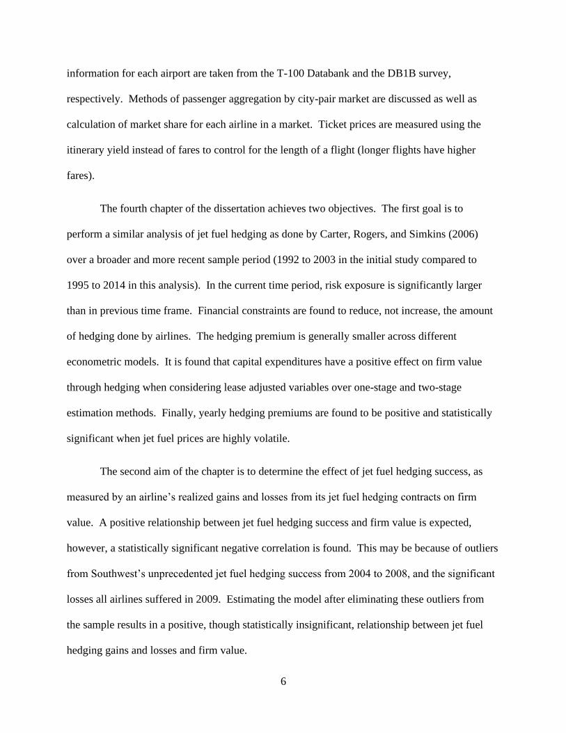
The fourth chapter of the dissertation achieves two objectives. The first goal is to

perform a similar analysis of jet fuel hedging as done by Carter, Rogers, and Simkins (2006)

over a broader and more recent sample period (1992 to 2003 in the initial study compared to

1995 to 2014 in this analysis). In the current time period, risk exposure is significantly larger

than in previous time frame. Financial constraints are found to reduce, not increase, the amount

of hedging done by airlines. The hedging premium is generally smaller across different

econometric models. It is found that capital expenditures have a positive effect on firm value

through hedging when considering lease adjusted variables over one-stage and two-stage

estimation methods. Finally, yearly hedging premiums are found to be positive and statistically

significant when jet fuel prices are highly volatile.

The second aim of the chapter is to determine the effect of jet fuel hedging success, as

measured by an airline’s realized gains and losses from its jet fuel hedging contracts on firm

value. A positive relationship between jet fuel hedging success and firm value is expected,

however, a statistically significant negative correlation is found. This may be because of outliers

from Southwest’s unprecedented jet fuel hedging success from 2004 to 2008, and the significant

losses all airlines suffered in 2009. Estimating the model after eliminating these outliers from

the sample results in a positive, though statistically insignificant, relationship between jet fuel

hedging gains and losses and firm value.

7

Chapter five discusses how successful jet fuel hedging can affect an airline’s business

decisions regarding expansion versus bolstering markets where the airline already operates.

Airlines with increased cash flows from jet fuel hedges may choose to return the savings to

shareholders as dividends, lower their ticket fares to increase market share in existing markets, or

choose to enter new markets. A simple model is used to test the correlation between positive jet

fuel hedging gains and market share (share of passengers flown by an airline in a market relative

to the total number of passengers flown across all airlines in the market). The primary airline

studied is Southwest Airlines because of their significant jet fuel hedging gains in the early to

mid-2000s followed by hedging losses after 2009. A positive and statistically significant

relationship is found between positive hedging gains and market share across multiple market

restrictions and definitions.

Chapter six concludes the dissertation by discussing the primary findings and

contributions to the hedging and antitrust literature made by this dissertation. Three

contributions are made in chapter four. First, jet fuel hedging gains and losses are found to have

a negative and statistically significant effect on firm value. However, this relationship becomes

positive after the elimination of outliers from the sample. Second, the section regarding the

determinants of jet fuel hedging find a negative relationship between financial constraint

variables and the amount of jet fuel hedging. This provides more evidence that suggests

financially constrained firms hedge less, not more. Third, a positive association between capital

expenditures and the hedging premium is found when accounting for aircraft leases. Without

adjusting for leases, the correlation is negative and statistically insignificant. This shows that

investing in leased aircraft is an important component of the additional value airlines can gain

from capital expenditures.

8

The primary contribution in chapter five is finding a positive and statistically significant

relation between successful jet fuel hedging and changes in market share for Southwest Airlines.

Although this does not suggest that Southwest is necessarily buying market share, it does show

that further investigation is warranted.

9

Figure 1.1: Spot Prices for US Gulf Coast Jet Fuel and WTI Crude Oil

Notes: This graph shows the spot prices for US Gulf Coast Jet Fuel and WTI Crude Oil from

April 1990 to May 2018 in dollars per barrel. Jet fuel spot prices were converted from dollars

per gallon to dollars per barrel by multiplying dollars per gallon by 42. Source: Energy and

Information Administration, https://www.eia.gov/.

0

20

40

60

80

100

120

140

160

180A

pr-

19

90

Ap

r-1

99

1

Ap

r-1

99

2

Ap

r-1

99

3

Ap

r-1

99

4

Ap

r-1

99

5

Ap

r-1

99

6

Ap

r-1

99

7

Ap

r-1

99

8

Ap

r-1

99

9

Ap

r-2

00

0

Ap

r-2

00

1

Ap

r-2

00

2

Ap

r-2

00

3

Ap

r-2

00

4

Ap

r-2

00

5

Ap

r-2

00

6

Ap

r-2

00

7

Ap

r-2

00

8

Ap

r-2

00

9

Ap

r-2

01

0

Ap

r-2

01

1

Ap

r-2

01

2

Ap

r-2

01

3

Ap

r-2

01

4

Ap

r-2

01

5

Ap

r-2

01

6

Ap

r-2

01

7

Ap

r-2

01

8

Spo

t P

rice

(D

olla

rs/B

arre

l)Spot Prices for US Gulf Coast Jet Fuel and

WTI Crude Oil (1990-2018)

US Gulf Coast Jet Fuel WTI Crude Oil

https://www.eia.gov/

10

Table 1.1: Yearly Jet Fuel Expense as a Percent of Total Operating Expense

Airline

Year American Alaska Delta JetBlue Southwest United Average

2001 14.87% 15.77% 13.25% 14.71% 16.89% 14.19% 14.95%

2002 13.81% 14.26% 12.89% 15.09% 16.21% 12.00% 14.04%

2003 16.44% 16.14% 14.89% 18.76% 16.53% 14.87% 16.27%

2004 22.70% 21.53% 19.20% 23.50% 18.26% 18.03% 20.54%

2005 28.87% 25.60% 26.64% 31.55% 21.49% 24.11% 26.38%

2006 31.47% 28.64% 27.50% 35.61% 28.00% 31.36% 30.43%

2007 32.06% 28.24% 27.88% 37.06% 29.87% 32.47% 31.26%

2008 38.76% 39.43% 34.46% 43.73% 37.26% 42.58% 39.37%

2009 28.25% 22.94% 27.92% 33.76% 32.36% 27.68% 28.82%

2010 30.67% 28.90% 27.55% 34.63% 34.53% 32.61% 31.48%

2011 35.60% 36.22% 31.01% 42.05% 40.03% 37.33% 37.04%

2012 37.22% 37.79% 31.25% 41.26% 39.64% 38.34% 37.58%

2013 37.71% 36.24% 35.48% 39.94% 37.26% 35.45% 37.01%

2014 34.94% 34.23% 37.88% 37.91% 34.56% 33.93% 35.58%

Notes: This table shows the yearly jet fuel expense as a percentage of total operating expense

from 2001 to 2014 for six major United States airlines and the overall average for all six airlines.

11

CHAPTER TWO:

LITERATURE REVIEW OF JET FUEL HEDGING IN THE AIRLINE INDUSTRY

2.1 Introduction to the Hedging Literature

People and firms have used hedging as a financial and economic tool to protect against economic

uncertainty for centuries. As noted by Smith and Stulz (1985, p. 391), hedging strategies

employed by firms had been well documented in the literature previous to their work. However,

the effect that hedging has on firm and industry performance had received very little academic

scrutiny up to that point. Since the publication of their work, the role of hedging on firm

behavior and performance has become a topic of significant theoretical and empirical interest.

2.1.1 Theoretical Hedging Literature Overview

The theoretical hedging literature asks several fundamental questions: What firm characteristics

affect the firm’s decision or ability to hedge or not? If the firm does hedge, how much does it

hedge? How does hedging affect the value of the firm? To what extent does a hedging firm

affect its value compared to a non-hedging firm? The theories developed to answer these

questions are separated into multiple categories. Financial constraint theories determine how

firms approach their hedging decisions when they are in financial distress (or simply in danger of

entering distress). Smith and Stulz (1985) and Rampini, Sufi, and Viswanathan (2014) are the

major theoretical studies that deal with the hedging behavior of financially distressed firms.

Firms facing severe financial constraints may suffer from underinvestment, that is, firms with

12

insufficient leverage may be unable to secure external financing to fund profitable investment

projects. Such firms may hedge more to increase internal cash flows, allowing for profitable

investment and increasing the value of the firm. Froot, Scharfstein, and Stein (1993) primarily

explores this underinvestment theory of hedging.

The tax structure of the firm also plays a role in a firm’s decision to hedge and hedging’s

impact on value. Smith and Stulz (1985) explain that firms with convex tax functions with

respect to value can expect higher firm values when hedging as a result of reduced expected tax

liability. The degree of tax function convexity may influence the amount of hedging engaged in

by firms to take advantage of a reduced expected tax liability. Finally, Smith and Stulz (1985)

show that managerial compensation may affect hedging decisions. Firms have an incentive to

offer managerial compensation packages whose incentives align with those of the firm.

Otherwise, the firm may create agency problems if compensation incentives do not match the

firm’s objectives.

2.1.2 Empirical Hedging Literature Overview

Numerous empirical studies have been performed to test hypotheses developed in the theoretical

hedging literature. These studies cover multiple industries and different sources of risk (e.g.,

commodity prices, foreign currencies, interest rates, etc.). For example, Tufano (1996) analyzes

gold price hedging by gold mining firms, Haushalter (2000) and Jin and Jorion (2006) observe

output price hedging by oil and gas firms, Carter, Rogers, and Simkins (2006) investigate jet fuel

hedging by airlines, and Allyannis and Weston (2001) evaluate foreign currency hedging by

nonfinancial firms.

13

The analyses that evaluate the factors that influence firm hedging decisions find that

financial constraints and managerial compensation are the most important determinants of

hedging by firms while tax considerations are generally insignificant. Studies on the effect of

hedging on firm value show mixed results. Allyannis and Weston (2001) and Carter, Rogers,

and Simkins (2006) both find a positive relationship between hedging and firm value while Jin

and Jorion (2006) determine no statistical effect.

2.1.3 Jet Fuel Hedging Literature Overview

One of the seminal papers in the hedging literature is the Carter, Rogers, and Simkins (2006)

study of jet fuel hedging in the airline industry. They find that the airline industry fits the

underinvestment framework of Froot, Scharfstein, and Stein (1993) because of airlines high

distress costs and positive relationship between investment and jet fuel prices. They evaluate the

determinants of jet fuel hedging by airlines and the effect that jet fuel hedging has on the value of

the airline. Finally, they show that the source of value from hedging comes capital expenditures

which is again consistent with the Froot, Scharfstein, and Stein (1993) theory of hedging.

Further studies of jet fuel hedging in the airline industry investigate jet fuel hedging by

using operational hedging (Treanor, et al., 2014a). This is primarily done by using more fuel-

efficient aircraft and maintaining a diverse fleet by aircraft size. Treanor, et al. (2014b) evaluate

how airline adjust their jet fuel hedging behavior as the jet fuel price exposure of changes and

estimate the effect of jet fuel hedging on firm value over different levels of jet fuel price

exposure.

The remainder of the literature review is structured as follows. Section 2.2 provides

greater detail of the theoretical hedging literature and possible discrepancies in different theories.

14

Section 2.3 discusses the empirical literature of hedging and how the results of the studies

comport with the theories described in section 2.2. Section 2.4 focuses on studies of jet fuel

hedging in the airline industry, what influences jet fuel hedging decisions, and how it affects the

value of the firm. Section 2.5 offers suggestions on further avenues of research proposed by

Carter, et al. (2017).

2.2 Theoretical Literature: Hedging and Firm Value

Firms use hedging as a way to reduce risk due to unexpected fluctuations in different kinds of

economic variables. Smith and Stulz (1985) define hedging as a reduction in the dependence of

firm value on changes in a state variable. Vasigh, Fleming, and Humphries (2014) define the

objective of hedging as the reduction or minimization of price risk resulting from uncertainty in

future price levels. Firms typically engage in hedging by buying or selling financial derivatives

such as future contracts, forward contracts, options (input price hedgers will generally use call

options, output price hedgers will generally use put options), and swaps.

Since financial derivatives that firms use to hedge against input price risk have zero

expected value, and investors can hold diversified portfolios to avoid higher rates of risk, one can

sensibly ask how engaging in hedging can have a non-zero effect on firm value? Modigliani and

Miller (1958) show that the value of the firm is independent of the capital structure used to

finance the firm. This is true, however, only when markets are efficient and there are no taxes,

financial distress costs, agency costs, or asymmetric information, none of which are generally

true in practice. Several theories have been introduced to explain how the existence of these

market imperfections allow hedging to increase firm value.

15

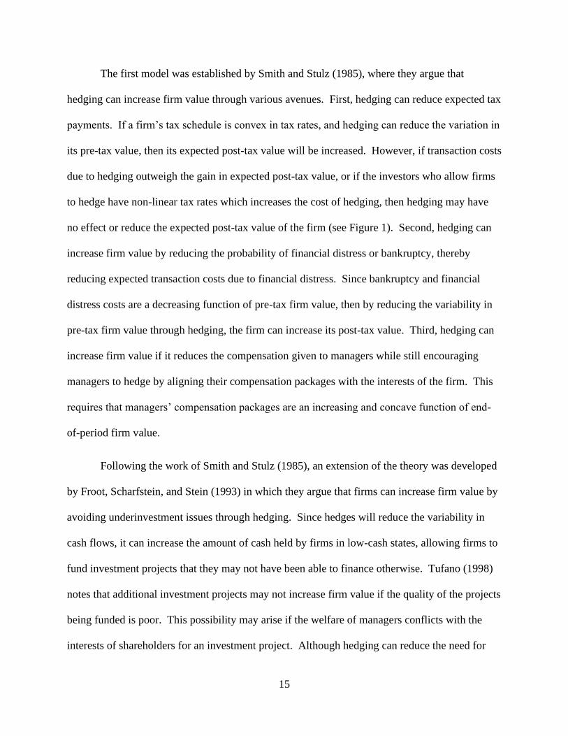
The first model was established by Smith and Stulz (1985), where they argue that

hedging can increase firm value through various avenues. First, hedging can reduce expected tax

payments. If a firm’s tax schedule is convex in tax rates, and hedging can reduce the variation in

its pre-tax value, then its expected post-tax value will be increased. However, if transaction costs

due to hedging outweigh the gain in expected post-tax value, or if the investors who allow firms

to hedge have non-linear tax rates which increases the cost of hedging, then hedging may have

no effect or reduce the expected post-tax value of the firm (see Figure 1). Second, hedging can

increase firm value by reducing the probability of financial distress or bankruptcy, thereby

reducing expected transaction costs due to financial distress. Since bankruptcy and financial

distress costs are a decreasing function of pre-tax firm value, then by reducing the variability in

pre-tax firm value through hedging, the firm can increase its post-tax value. Third, hedging can

increase firm value if it reduces the compensation given to managers while still encouraging

managers to hedge by aligning their compensation packages with the interests of the firm. This

requires that managers’ compensation packages are an increasing and concave function of end-

of-period firm value.

Following the work of Smith and Stulz (1985), an extension of the theory was developed

by Froot, Scharfstein, and Stein (1993) in which they argue that firms can increase firm value by

avoiding underinvestment issues through hedging. Since hedges will reduce the variability in

cash flows, it can increase the amount of cash held by firms in low-cash states, allowing firms to

fund investment projects that they may not have been able to finance otherwise. Tufano (1998)

notes that additional investment projects may not increase firm value if the quality of the projects

being funded is poor. This possibility may arise if the welfare of managers conflicts with the

interests of shareholders for an investment project. Although hedging can reduce the need for

16

external financing, the scrutiny provided by capital markets may reduce the likelihood that

proposed investment projects destroy value. Increasing internal financing by hedging can

increase the expected number of value-destroying projects that would not otherwise be funded by

investors outside the firm.

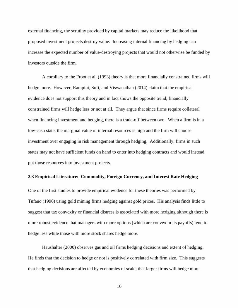
A corollary to the Froot et al. (1993) theory is that more financially constrained firms will

hedge more. However, Rampini, Sufi, and Viswanathan (2014) claim that the empirical

evidence does not support this theory and in fact shows the opposite trend; financially

constrained firms will hedge less or not at all. They argue that since firms require collateral

when financing investment and hedging, there is a trade-off between two. When a firm is in a

low-cash state, the marginal value of internal resources is high and the firm will choose

investment over engaging in risk management through hedging. Additionally, firms in such

states may not have sufficient funds on hand to enter into hedging contracts and would instead

put those resources into investment projects.

2.3 Empirical Literature: Commodity, Foreign Currency, and Interest Rate Hedging

One of the first studies to provide empirical evidence for these theories was performed by

Tufano (1996) using gold mining firms hedging against gold prices. His analysis finds little to

suggest that tax convexity or financial distress is associated with more hedging although there is

more robust evidence that managers with more options (which are convex in its payoffs) tend to

hedge less while those with more stock shares hedge more.

Haushalter (2000) observes gas and oil firms hedging decisions and extent of hedging.

He finds that the decision to hedge or not is positively correlated with firm size. This suggests

that hedging decisions are affected by economies of scale; that larger firms will hedge more

17

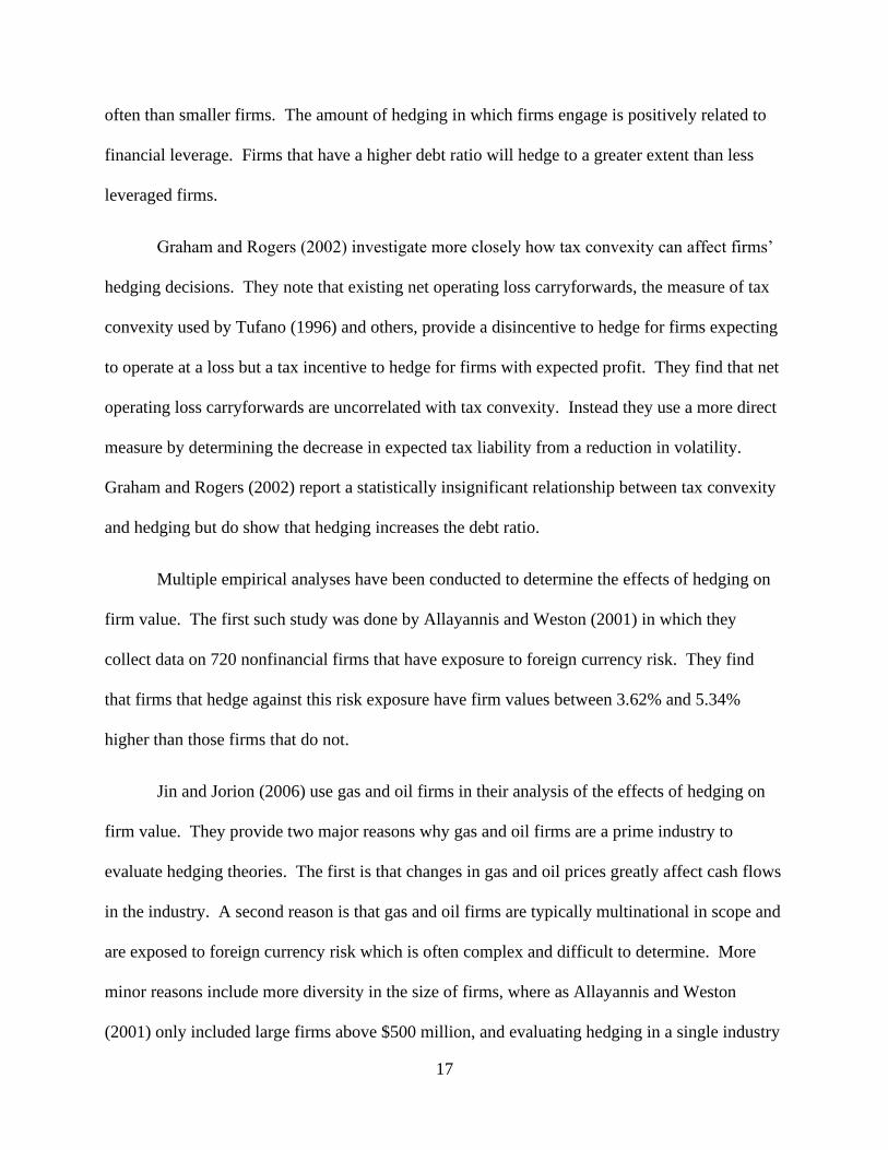
often than smaller firms. The amount of hedging in which firms engage is positively related to

financial leverage. Firms that have a higher debt ratio will hedge to a greater extent than less

leveraged firms.

Graham and Rogers (2002) investigate more closely how tax convexity can affect firms’

hedging decisions. They note that existing net operating loss carryforwards, the measure of tax

convexity used by Tufano (1996) and others, provide a disincentive to hedge for firms expecting

to operate at a loss but a tax incentive to hedge for firms with expected profit. They find that net

operating loss carryforwards are uncorrelated with tax convexity. Instead they use a more direct

measure by determining the decrease in expected tax liability from a reduction in volatility.

Graham and Rogers (2002) report a statistically insignificant relationship between tax convexity

and hedging but do show that hedging increases the debt ratio.

Multiple empirical analyses have been conducted to determine the effects of hedging on

firm value. The first such study was done by Allayannis and Weston (2001) in which they

collect data on 720 nonfinancial firms that have exposure to foreign currency risk. They find

that firms that hedge against this risk exposure have firm values between 3.62% and 5.34%

higher than those firms that do not.

Jin and Jorion (2006) use gas and oil firms in their analysis of the effects of hedging on

firm value. They provide two major reasons why gas and oil firms are a prime industry to

evaluate hedging theories. The first is that changes in gas and oil prices greatly affect cash flows

in the industry. A second reason is that gas and oil firms are typically multinational in scope and

are exposed to foreign currency risk which is often complex and difficult to determine. More

minor reasons include more diversity in the size of firms, where as Allayannis and Weston

(2001) only included large firms above $500 million, and evaluating hedging in a single industry

18

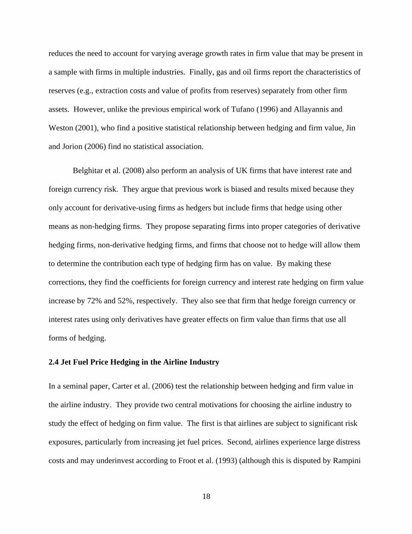
reduces the need to account for varying average growth rates in firm value that may be present in

a sample with firms in multiple industries. Finally, gas and oil firms report the characteristics of

reserves (e.g., extraction costs and value of profits from reserves) separately from other firm

assets. However, unlike the previous empirical work of Tufano (1996) and Allayannis and

Weston (2001), who find a positive statistical relationship between hedging and firm value, Jin

and Jorion (2006) find no statistical association.

Belghitar et al. (2008) also perform an analysis of UK firms that have interest rate and

foreign currency risk. They argue that previous work is biased and results mixed because they

only account for derivative-using firms as hedgers but include firms that hedge using other

means as non-hedging firms. They propose separating firms into proper categories of derivative

hedging firms, non-derivative hedging firms, and firms that choose not to hedge will allow them

to determine the contribution each type of hedging firm has on value. By making these

corrections, they find the coefficients for foreign currency and interest rate hedging on firm value

increase by 72% and 52%, respectively. They also see that firm that hedge foreign currency or

interest rates using only derivatives have greater effects on firm value than firms that use all

forms of hedging.

2.4 Jet Fuel Price Hedging in the Airline Industry

In a seminal paper, Carter et al. (2006) test the relationship between hedging and firm value in

the airline industry. They provide two central motivations for choosing the airline industry to

study the effect of hedging on firm value. The first is that airlines are subject to significant risk

exposures, particularly from increasing jet fuel prices. Second, airlines experience large distress

costs and may underinvest according to Froot et al. (1993) (although this is disputed by Rampini

19

et al. (2014)). Airlines can hedge against jet fuel price risk and possibly avoid the

underinvestment problem.

Carter et al (2006) first quantify airlines’ jet fuel price risk exposure which they measure

in two ways. They begin by analyzing the relationship between jet fuel prices and airlines’

stock price by running a time-series regression on the monthly equally weighted rate of return for

the sample of airlines on the percent changes in jet fuel prices and the rate of return on the

market portfolio. They find a statistically significant negative effect of changes in jet fuel prices

on stock value. A one standard deviation change in jet fuel prices - 15.7 cents from 1994 to 2003

- would result in a 2.75% change in stock value. The second measure of jet fuel price risk they

examine is cash flow sensitivity on a three standard deviation change in jet fuel prices. A typical

airline would experience a 91% decrease in the possible value of investment if a three standard

deviation rise in jet fuel prices were to occur. An airline that hedges 24% of next year’s jet fuel

requirements would result in 21.7% additional cash flow relative to yearly capital expenditures

compared to an airline that does not hedge.

Carter et al. (2006) go on to demonstrate that the airline industry follows the Froot et al.

(1993) investment framework through multiple statistical analyses. They show with a univariate

analysis that jet fuel prices and cash flow are negatively correlated (ρ = -0.487 from 1986 to

2003) while the correlation between jet fuel prices and capital expenditures is positive (ρ = 0.464

from 1979 to 2003). Next, they perform a regression of capital expenditures scaled by lagged

assets on inflation-adjusted jet fuel price per gallon, cash flow scaled by lagged assets, and

lagged Tobin’s Q. They find that the coefficient for inflation-adjusted jet fuel price per gallon to

be positive and statistically significant, suggesting greater investment opportunities during

20

periods of higher jet fuel prices. Hedging jet fuel prices would allow for airlines to better fund

investment during these periods by decreasing the variability in cash flows.

Carter et al. (2006) investigate the factors that may influence an airline’s decision to

hedge based on the theories of Froot et al. (1993) and Smith and Stulz (1985). They consider the

effects of financial constraints, tax convexity, and managerial incentives to adjust firm risk on jet

fuel hedging decisions. Other factors that may affect jet fuel hedging decisions are included,

such as different types of financial hedges (e.g., interest rates and foreign currencies) and other

methods of reducing jet fuel price risk (e.g., fuel pass-through agreements and charter

operations).

Variables from each of these categories are regressed on two measures of jet fuel hedging

by airlines. The first measures the extent of jet fuel hedging, as measured by the percentage of

next year’s jet fuel requirements hedged. Second, airlines’ decision to hedge or not to hedge,

measured by an indicator which is one if the airline hedges a positive amount of next year’s jet

fuel requirements and zero otherwise. Carter et al. (2006) find that the factors which best explain

the degree to which airlines hedge jet fuel prices match the underinvestment theory of Froot et al.

(1993). However, explanatory power of the variables relevant to the underinvestment framework

vanish for the model in which the indicator for jet fuel hedging decisions is used.

Next, Carter et al. (2006) explore how jet fuel hedging may affect firm value. The value

of the firm is measured by Tobin’s Q. The percentage of next year’s fuel requirements hedged

and an indicator for positive jet fuel hedging quantify the amount of jet fuel hedging and an

airline’s jet fuel hedging decision, respectively. They observe that an airline that hedges all of

next year’s jet fuel requirements has a hedging premium (i.e., an increase in firm value) of nearly

35%. For airlines that have a positive amount of jet fuel hedges in place, the average percentage

21

of next year’s fuel requirements hedged is approximately 29.4%. An airline that hedges jet fuel

prices at the average has a hedging premium of 10.2%.

A potential source of the hedging premium is examined by seeing how an interaction of

capital expenditures (which is a measure of investment by an airline) and jet fuel hedging affects

firm value. Carter et al. (2006) find a positive and significant relationship between this

interaction and firm value which shows that investment is more valuable to firms that hedge jet

fuel prices than firms that do not. They find a hedging premium of almost 20.7%, nearly all of

which comes from its effect on investment through capital expenditures.

In their discussion on the factors that contribute to the decision to hedge, Carter et al.

(2006) note that some variables related to financial constraints (e.g., cash flow-to-sales and credit

rating) show the opposite effect predicted by Froot et al. (2003). Whereas previous theory

suggests more financially constrained airlines should hedge more, their analysis indicates that

those airlines hedge less. Morrell and Swan (2006) argue that airlines that are in financial

distress may desire to hedge but are unable since entering into hedging contracts is costly.

Rampini et al. (2014), in addition to providing a theoretical basis for explaining why financially

constrained firms are less likely to hedge, counter to the claims made by Froot et al. (1993), they

also provide empirical support for their theory. They find that in the year before entering distress

and the period of distress, the percent of fuel hedged for the following year decreases from an

average of 25% to an average of 5%. They also acknowledge that airlines also understand this

dynamic, as airlines consistently cite distress and the resulting collateral constrains as a reason

why they do not engage in hedging.

More recent studies in the hedging literature have focused on airlines’ exposure to jet fuel

price risk. In a general financial sense, risk is the probability that the value of a financial item

22

will change whereas exposure is the variance of the value the financial item due of the risk. In

the current context, jet fuel price risk is the probability that jet fuel prices will change while the

exposure to jet fuel prices describe how sensitive the firm value of an airline is to changes in the

price of jet fuel.

Treanor et al. (2014a) provide a rational for analyzing risk and exposure from jet fuel

prices by arguing that airlines inherently benefit from falling jet fuel prices. Unlike exposure due

to jet fuel, foreign currency exposure depends on whether a firm is an importer or exporter on

net, while interest rate exposure depends on the firm’s status as a net borrower or lender. The

second reason is that jet fuel costs have increased as a total share of airlines’ total expenses over

time. The third reason is that the price of jet fuel is far more volatile than foreign currency

exchange rates and interest rates.

Treanor et al. (2014a) separate an airline’s hedging activities into two major types of

hedges: financial hedges and operational hedges. Financial hedges (discussed previously)

involve the use of financial derivatives to protect against possible increases in the price of jet

fuel. Operational hedges most commonly take the form of more fuel-efficient aircraft (by

aircraft age) and fleet diversification (by aircraft size). Flying newer aircraft that are

comparatively more fuel-efficient than older aircraft reduces the amount of fuel needed to fly the

same number of routes, which then reduces the negative impact on the airline’s profit when fuel

prices are high. Similarly, when an airline maintains a diverse fleet with different sizes of

aircraft (with each having differing fuel capacities), the airline can switch to smaller aircraft

when fuel prices are high to reduce overall fuel expense. Although the airline may sacrifice

economies of scale associated with larger aircraft, it may be more costly to continue to operate

large aircraft or leave the market completely and reenter at a later time than to operate smaller

23

aircraft at a loss. Operational hedges can still benefit airlines even when jet fuel prices are low,

while financial hedges generally cannot. However, operational hedging can be more costly than

financial hedges because of the high capital cost of acquiring additional aircraft and the

considerable maintenance costs of maintaining a diverse fleet. When comparing the reduction in

exposure to financial and operational hedging, Treanor et al. (2014a) find that a one percent

increase in the amount of fuel hedged in the next year reduces jet fuel price exposure by 1%.

Alternatively, a one-year reduction in fleet age or a 1% increase in fleet fuel efficiency can

reduce fuel risk exposure by 2.3% and 11%, respectively.

Treanor, et. al. (2014b) expand on the work of Carter, et. al. (2006) by including jet fuel

exposure in airlines’ hedging decisions and how changes in hedging behavior due to jet fuel

exposure affects firm value. They first find that airlines that are subject to greater jet fuel

exposure hedge more. Airlines that have an 8.5% increase in jet fuel exposure hedge on average

10.7% more of next year’s expected jet fuel requirements. However, the increase in hedging

when jet fuel exposure is high has no association with an increase in the firm value of airlines.

They suggest that airlines simply value hedging jet fuel prices generally and not necessarily

selective hedging during times of high jet fuel exposure.

2.5 Overview of Commodity Price Hedging

Carter et al. (2017) attempt to aggregate the general findings of the commodity risk management

literature and provide possible directions for future research. Beginning with the Modigliani and

Miller theorem in which hedging cannot increase the value of the firm in perfect and efficient

markets, numerous authors have shown that in the absence of this perfect world, investors can

value hedging through a multitude of avenues. Changes in accounting standards have led to an

improvement in data availability which allows investigators to more easily analyze questions

24

involving hedging decisions and their impact on the firm. They note that empirical findings

regarding hedging decisions may depend on the industry being analyzed or whether the firms

examined are producers or users of the commodity, as well as differences in economic conditions

of the time periods studied.

Carter et al. (2017) suggest multiple questions that future research can consider. In

particular are concerns about differences in results between industries and replication of results

within industries over different time periods. Studies on corporate culture may be necessary and

mergers between firms or changes in management can change hedging decisions and strategies.

Finally, they suggest that research should be able to help businesses with the decision to hedge or

not, and if so how much. Field-based case studies may provide valuable insight into how firms

actually make hedging decisions.

25

CHAPTER 3:

DATA SOURCES AND COLLECTION

3.1 Database Overview

The data for the analyses performed in this dissertation come from three sources. General

financial data are found in the Compustat database. This database is maintained by Wharton

Research Data Services (WRDS) within the Wharton School of the University of Pennsylvania.

Data for risk management strategies used by airlines are manually recorded from Securities and

Exchange Commission (SEC) 10-K statements.3 These filings are publicly available on the

Electronic Data Gathering, Analysis, and Retrieval system (EDGAR) maintained by the SEC.

Airline passenger data and ticket fare data are taken from Air Carrier Statistics (T-100) database

and the Airline Origin and Destination (DB1B) survey, respectively. The Office of Airline

Information of the Bureau of Transportation Statistics (BTS) manages both databases. Each of

the two databases can be found on the Transtats website, also maintained by the BTS.4

Each section of this chapter provides a detailed discussion of the data collection methods

and calculations for the variables obtained from each database. Section 3.2 describes the

variable names and locations of financial data within Compustat and the different company

codes that can be used to identify airlines within the database. Section 3.3 shows how to collect

3 The SEC describes Form 10-K as a document that provides a comprehensive overview of a company’s business

and financial condition and includes audited financial statements. 4 https://www.transtats.bts.gov/

26

jet fuel hedging data within airline 10-K statements. This includes information on the amount of

hedging airlines engage in and the gains and losses airlines receive from those hedges. Examples

of jet fuel hedging reporting by airlines in selected 10-K statements are given. Data for other

risk management strategies, such as interest rate hedges and fuel pass-through agreements, are

also covered. Section 3.4 demonstrates how passenger and ticket fare data for each airline are

aggregated across different markets and time intervals (e.g., total passengers flown yearly,

quarterly, etc. for an origin/destination pair).

3.2 Compustat Database

Most financial variables are found in Compustat under North America – Annual Updates –

Fundamentals Annual. These items are separated in multiple categories: balance sheet items,

income statement items, cash flow items, miscellaneous items, and supplemental data items.

Table 3.1 shows the variable name, the category the variable can be found in the Compustat

Fundamentals Annual database, and the item name. Credit rating variables can be found in

Compustat under North America – Annual Updates – Ratings in the “Data Items” category. S&P

Long Term Issuer Credit Rating is selected as the credit rating variable used in the analyses.

Executive compensation variables are located in Compustat under Execucomp – Monthly

Updates – Annual Compensation. Total shares owned excluding options and the number of

options awarded are taken from the “Compensation Data” category. The Annual CEO Flag in

the “Executive Information” category indicates which executive was the CEO of the company

for most of the fiscal year.

Companies can be identified through six different types of company codes: ticker

symbol, GVKEY, CUSIP, SIC, NAICS, and CIK. The primary company identifier used is

27

GVKEY. Compustat permanently associates GVKEY with a single company over its entire life,

whereas the other company codes may be changed and reused over time. Each of these company

identifiers can be selected in any data query report under the “Identifying Information” grouping.

3.3 EDGAR Database

Financial hedging data are not directly available in any Compustat database. However,

information regarding a company’s financial hedging activities are reported in their annual 10-K

filings with the SEC. These filings are publicly accessible from the EDGAR database.

Documents available in EDGAR go back to 1994 filings. Airlines are identified in EDGAR with

their stock ticker symbols.

For any year in which a 10-K is not available, the company may have submitted a 10-

K405 filing. This form is identical to a 10-K form and is required to be filed if a director or other

officer of a company failed to submit Form 3, Form 4, or Form 5 on time to disclose any insider

trading activities. 10-K405 filings were discontinued after 2002.

3.3.1 Jet Fuel Hedging Measures from Form 10-K

An airline’s jet fuel hedging activities are measured in two ways: (1) by the percentage of an

airline’s expected jet fuel requirements for the next year hedged, and (2) the gains or losses from

an airline’s jet fuel hedges. The percentage of next year’s jet fuel requirements hedged measures

the amount of jet fuel hedging each airline engages in relative to its expected fuel requirements

for the following year, while the gains or losses from an airline’s jet fuel hedges measure the

performance of its jet fuel hedging activities.

28

3.3.1.1 Percentage of Next Year’s Jet Fuel Requirements Hedged

Airlines report the percentage of next year’s expected jet fuel requirements hedged in multiple

ways. Most airlines report the amount of jet fuel hedging as a yearly value. Southwest Airlines

(2004), for example, reported that it will hedge over 82 percent of fuel requirements for 2004.

The expected amount of fuel requirements hedged may also be given quarterly. Alaska Airlines

(2008), for example, reported hedges in place for approximately 50% of fuel requirements in the

first quarter of 2008, 38% in the second quarter, 33% in the third quarter, and 34% in the fourth

quarter (see Figure 3.1). Alaska also gives the full year expected fuel requirements hedged at

39%. This is the arithmetic average for each of the four quarters (rounded to the nearest whole

percent). When quarterly hedging values are given without a full year hedging value, the yearly

value is calculated as the arithmetic average of the percentage of jet fuel hedging for each of the

four quarters. Airlines may also report the expected number of gallons hedged. The

corresponding percentage of expected fuel requirements hedged is calculated by dividing

expected gallons hedged with total expected fuel requirements for the following year. For

example, Delta Air Lines (1999) disclosed that it expected to hedge 2.1 billion gallons of jet fuel

in 1999 and projected its fuel consumption for 1999 to be 2.7 billion gallons. This computes to a

percentage of next year’s expected jet fuel hedged of 76.9%.

Airlines may disclose jet fuel hedging activities not only for the next year, but also two or

three years into the future. These hedging activities beyond one year in the future are not

included in the data. Airlines may alter their hedging contracts for future years beyond the first.

In 2007, for example, Alaska Airlines had hedging contracts in place for 39% of its expected jet

fuel requirements for 2008 and 5% of its expected jet fuel requirements for 2009 (Alaska Air

29

Group, 2008).5 By 2008, it purchased additional hedging contracts for a total of 50% of its 2009

fuel requirements (Alaska Air Group, 2009).

It is important to note that not all practices that manage jet fuel price risk for an airline

are counted as hedges. Smaller airlines sometimes use fuel pass-through agreements to pass on

the cost of using jet fuel to a party other than the airline.6 These agreements do not alter the jet

fuel price risk borne by the airline, but simply pass on that risk to the other airline in the

agreement. For any year in which an airline does not have any financial derivatives in place to

hedge jet fuel price risk for the following year, its expected fuel requirements hedged for next

year will be zero, even if the airline passes on some or all of its jet fuel price risk to another

airline by using some type of fuel pass-through agreement. These types of non-hedging jet fuel

risk management activities are discussed in section 3.3.2.

3.3.1.2 Gains and Losses from Jet Fuel Hedges

Prior to 2001, the reporting gains and losses from jet fuel hedges in 10-K statements was

optional and reporting practices were inconsistent between airlines. In June of 1998, the

Financial Accounting Standards Board passed FAS 133, Accounting for Derivatives Instruments

and Hedging Activities, which required companies to report the fair value of their derivative

instruments on their balance sheet.7 All companies were required to adopt FAS 133 by January

1, 2001. If an airline engages in jet fuel hedging by using financial derivatives, it must report the

5 Figure 3.1 shows an example of how Alaska Airlines reports the expected fuel requirements hedged for multiple

years. 6 Types of fuel pass-through agreements include fixed-price and cap arrangements, fuel purchase agreements, airline

service agreements, code share agreements, capacity purchase agreements, and contract flying arrangements. 7 The fair value of a financial derivative is the value of the instrument if it were settled at a given time. This is often

referred to as the mark-to-market value of the instrument.

30

fair value of those derivatives as assets or liabilities on its balance sheet. FAS 133 guarantees

that data on gains and losses from jet fuel hedging is reliable and consistent between airlines.

Gains and losses from hedging are divided into four categories: realized gains and losses,

unrealized gains and losses, gains and losses from ineffective hedges, and gains and losses from

hedges that do not qualify for hedge accounting. Airlines report realized gains when a financial

derivative has been exercised and the underlying fuel has been consumed. These gains are

generally reported under fuel expense or are reclassified from accumulated other comprehensive

income (AOCI) into income as fuel expense. Unrealized gains and losses are changes in the

mark-to-market value of all financial derivatives that have not been exercised. Unrealized gains

and losses are commonly recognized under AOCI. Gains and losses from ineffective hedges are

declared as ineffective and documented as nonoperating income. For any hedges that do not

qualify for hedge accounting, gains and losses are also reported as nonoperating income. All

gains and losses are after-tax values.

Figure 3.2 shows an example of gains and losses classifications from United Airlines’ jet

fuel hedging activities in its 2014 10-K filing. United Airlines’ unrealized gains fall under

“Amount of Gain (Loss) Recognized in AOCI on Derivatives (Effective Potion)” which amounts

to a gain of $39 million in 2013 but a loss of $51 million in 2012.8 The airlines’ realized gains

and losses are classified under “Gain (Loss) Reclassified from AOCI into Income (Fuel Expense)

(Effective Potion).” 2013 shows a realized gain of $18 million and a $141 million realized loss

in 2012. The ineffective potion of jet fuel hedges is labeled as “Amount of Gain (Loss)

Recognized in Nonoperating income (expense): Miscellaneous, net (Ineffective Portion).”

8 Although losses are indicated as being enclosed in parentheses in this example, this is not always a consistent

reporting standard. Airlines can report gains in parentheses as well, so care must be taken when interpreting

hedging gains and losses.

31

Ineffective gains and losses were positive $5 million in 2013 but losses of $1 million in 2012.

Hedges that do not qualify for hedge accounting amount to a gain of $79 million and $38 million

in 2013 and 2012, respectively. These gains and losses fall under “Amount of Gain Recognized

in Nonoperating income (expense): Miscellaneous, net.”

3.3.2 Other Variables Taken from Form 10-K

Airline 10-K statements contain information on other types of risk management activities,

including interest rate hedges, foreign currency hedges, usage of fuel pass-through agreements,

and charter arrangements with other companies. Data for each of these types of risk

management are collected as indictors variables. Interest rate and foreign currency hedge

indicators are assigned a value of one if the airline uses interest rate or foreign currency hedges

at any time during the year and zero otherwise.9 The fuel pass-through agreement indicator and

charter indicator are given a value of one if an airline passes on its fuel costs to another airline or

maintains charter operations with at least one other airline, respectively, and zero otherwise.

3.4 Bureau of Transportation Statistics Databases

Airline passenger and ticket fare data are taken from databases managed by the Office of Airline

Information of the BTS. Passenger data are retrieved from the Air Carrier Statistics database,

also called the T-100 data bank, while ticket fare data are collected from the Airline Origin and

Destination Survey, commonly referred to as the DB1B survey.

9 The most common interest rate hedges used are swaps and interest rate caps, while swaptions and treasury lock

agreements are less commonly used. Foreign currency hedges include call and put options, collars, futures, and

swaps.

32

3.4.1 T-100 Data Bank

The T-100 data bank contains four distinct tables: T-100 domestic segment, T-100 domestic

market, T-100 international segment, and T-100 international market. The BTS defines a

segment as a pair of points served or scheduled to be served by a single stage of at least one

flight at any given time. Market data include passengers, freight, and/or mail that enplane and

deplane between two specific points while the flight number remains the same. Data in domestic

tables are comprised of all flights where both the origin and destination airports are within the

boundaries of the United States or its territories. International tables include flights where at

least one of the points of service is within the United States or its territories. This study only

uses passenger data from the domestic market table.

Passenger data are gathered monthly for each pair of origin and destination markets from

each reporting airline.10 Airlines are required to report passenger numbers for all flights. The

airline ID variable in the database is used to identify unique airlines. This five-digit identifier is

constant for each holder of a Certificate of Public Convenience and does not change over time.

In contrast, airline names, codes (e.g., AA for American Airlines), and holding

companies/corporations may change due to bankruptcies or mergers with other airlines. Markets

are identified by a five-digit market ID. Some markets, however, are served by multiple airports.

When an airline flies passengers at multiple airports within the same market, passenger data are

reported for each airport.

Passenger data are aggregated in two ways: by city-pair market and by year. The Federal

Aviation Administration defines a city pair as a city of origin and a corresponding destination

10 Reporting airlines must hold a Certificate of Public Convenience and Necessity issued by the U.S. Department of

Transportation and have at least $20 million in annual operating revenues.

33

city for flights to and from major metropolitan areas (“City Pairs,” 2018). In the dataset, flights

to and from two unique markets as defined by the T-100 market ID are defined as a city-pair

market. To assist in passenger data aggregation across city-pair markets, a new six-digit city-

pair market identifier is constructed so that it is independent of which market is the origin and

which market is the destination. First, a new three-digit market identifier is generated for each

market so that it is the same whether the market is an origin or destination. The city-pair market

identifier is created by using the maximum new market ID of the origin/destination pair as the

first three digits and the minimum new market ID of the same origin/destination pair as the

second three digits.11 This eliminates the possibility that two unique city-pair markets can have

the same city-pair market identifier.

Passengers are also aggregated within each city-pair market by year for each airline. The

yearly passengers flown by each airline in a city-pair market is calculated by summing the

number of passengers flown by an airline for each month of a given year across all observations

with the same city-pair market identifier. Any year and city-pair market in which an airline did

not fly any passengers is assigned a value of zero for that airline year.

The yearly passenger share for each airline in a city-pair market is calculated by taking

the ratio of the number of passengers flown by the airline and the total number of passengers

flown by all airlines in that city-pair market. Any airline that has flown zero passengers in a

city-pair market year is given a passenger share of zero. Passenger shares are expressed as a

percentage of total passengers with values ranging from 0 and 100.

11 For example, the Tampa, Florida market has a new market ID of 222 and Phoenix, Arizona has a new market ID

of 39. The city-pair market identifier for these two markets is 39222.

34

3.4.2 DB1B Survey

In contrast to the T-100 data bank which requires reporting airlines to submit detailed passenger

data for all flights every month, the DB1B surveys 10% of tickets from reporting airlines every

quarter. The DB1B survey is divided into three tables: DB1BCoupon, DB1BMarket, and

DB1BTicket. The DB1BMarket table supplies information regarding origin and destination

market IDs that the other two tables do not have. Since the market IDs in the DB1BMarket are

identical to the market IDs of the T-100 data bank, this allows for consolidation of the fare data

with the T-100 passenger data for any city-pair market.

Airlines in the DB1BMarket are not directly identified by the airline ID as in the T-100

data bank. Instead, three separate identifiers are employed: the reporting carrier, the operating

carrier, and the ticketing carrier. The reporting carrier is the airline that submits data to the

Office of Airline Information for any given passenger segment. The operating carrier is the

airline directly involved in the operation of the aircraft. The marketing carrier is the airline that

issues a flight reservation or ticket under a codeshare agreement.12 Since the operating carrier

submits data for the T-100 data bank, the operating carrier in the DB1BMarket table is used as

the airline identifier (Lundy, 2016). Since the operating carrier is identified using the

International Air Transport Association (IATA) airline designator (e.g., AA for American

Airlines) instead of the airline ID identifier in the T-100, the IATA airline designator is

converted to the corresponding airline ID identifier.

The price of a flight is usually given by the ticket fare for the flight. Using this measure

of price may introduce bias as longer flights will generally have higher fares. This bias can be

12 A code share agreement is an arrangement in which one airline puts its IATA two-letter code on a flight operated

by a different airline (“Code Share Fact Sheet”).

35

corrected by using the ticket fare per mile flown as the price of a flight.13 The DB1B survey

presents this measure of ticket price as the total itinerary yield, which is defined as the itinerary

fare (i.e., the ticket fare) divided by the itinerary miles flown (e.g., the number of miles flown

between the origin and destination). In the DB1BMarket table, however, the itinerary yield is

not given directly. Instead, the itinerary fare (market fare) and the itinerary miles flown (market

miles flown) are provided. This allows the itinerary yield for each ticket to be computed by

taking the ratio of the market fare and the market miles flown. The average itinerary yield is

used as the average price of a ticket for each airline in a city-pair market. The average itinerary

yield is calculated as the weighted average of the itinerary yields for each origin/destination

combination within a city-pair market.14

13 This does not account for other factors that can introduce sampling bias, including seasonal fare differences and

fare class differences (e.g., first class, business class, economy, etc.). 14 A weighted average is used because the number of tickets surveyed for each origin/destination pair may be

different. If the number of tickets surveyed for flights from Tampa, Florida to Phoenix, Arizona is 100, and the

number of tickets surveyed on flights from Phoenix to Tampa is 150, then the weight on the two average itinerary

yields will be 0.4 (100/250) and 0.6 (150/250), respectively.

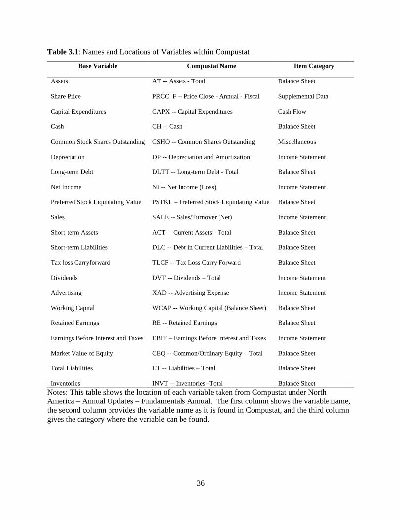
36

Table 3.1: Names and Locations of Variables within Compustat

Base Variable

Compustat Name Item Category

Assets

AT -- Assets - Total Balance Sheet

Share Price

PRCC_F -- Price Close - Annual - Fiscal Supplemental Data

Capital Expenditures

CAPX -- Capital Expenditures Cash Flow

Cash

CH -- Cash Balance Sheet

Common Stock Shares Outstanding

CSHO -- Common Shares Outstanding Miscellaneous

Depreciation

DP -- Depreciation and Amortization Income Statement

Long-term Debt

DLTT -- Long-term Debt - Total Balance Sheet

Net Income

NI -- Net Income (Loss) Income Statement

Preferred Stock Liquidating Value

PSTKL – Preferred Stock Liquidating Value Balance Sheet

Sales

SALE -- Sales/Turnover (Net) Income Statement

Short-term Assets

ACT -- Current Assets - Total Balance Sheet

Short-term Liabilities

DLC -- Debt in Current Liabilities – Total Balance Sheet

Tax loss Carryforward

TLCF -- Tax Loss Carry Forward Balance Sheet

Dividends

DVT -- Dividends – Total Income Statement

Advertising

XAD -- Advertising Expense Income Statement

Working Capital

WCAP -- Working Capital (Balance Sheet) Balance Sheet

Retained Earnings

RE -- Retained Earnings Balance Sheet

Earnings Before Interest and Taxes

EBIT – Earnings Before Interest and Taxes Income Statement

Market Value of Equity

CEQ -- Common/Ordinary Equity – Total Balance Sheet

Total Liabilities

LT -- Liabilities – Total Balance Sheet

Inventories INVT -- Inventories -Total Balance Sheet

Notes: This table shows the location of each variable taken from Compustat under North

America – Annual Updates – Fundamentals Annual. The first column shows the variable name,

the second column provides the variable name as it is found in Compustat, and the third column

gives the category where the variable can be found.

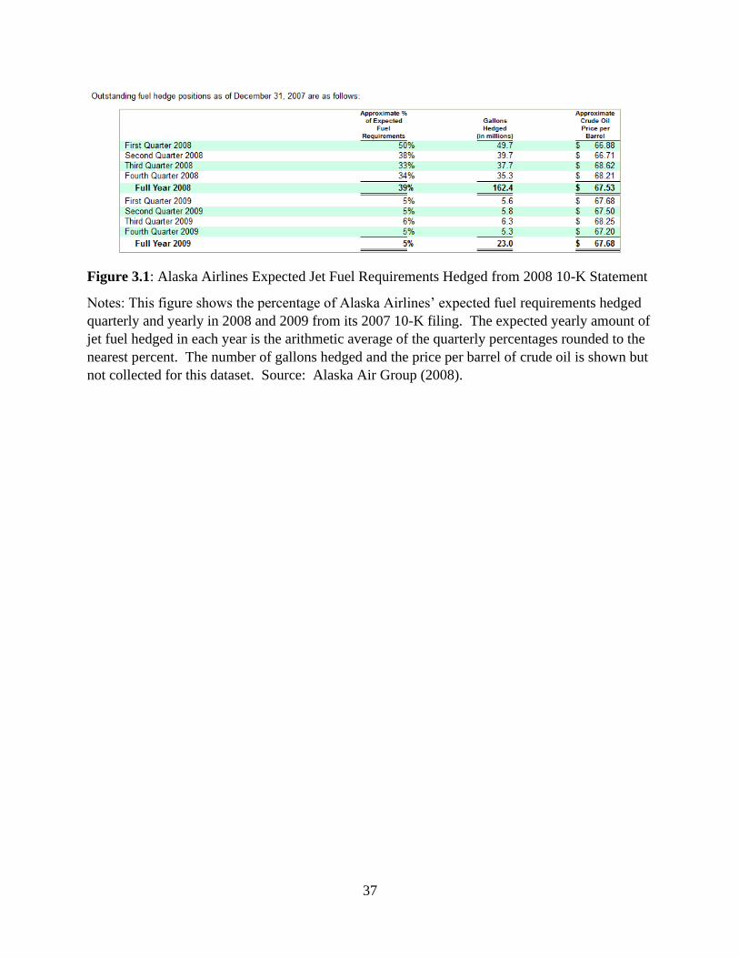
37

Figure 3.1: Alaska Airlines Expected Jet Fuel Requirements Hedged from 2008 10-K Statement

Notes: This figure shows the percentage of Alaska Airlines’ expected fuel requirements hedged

quarterly and yearly in 2008 and 2009 from its 2007 10-K filing. The expected yearly amount of

jet fuel hedged in each year is the arithmetic average of the quarterly percentages rounded to the

nearest percent. The number of gallons hedged and the price per barrel of crude oil is shown but

not collected for this dataset. Source: Alaska Air Group (2008).

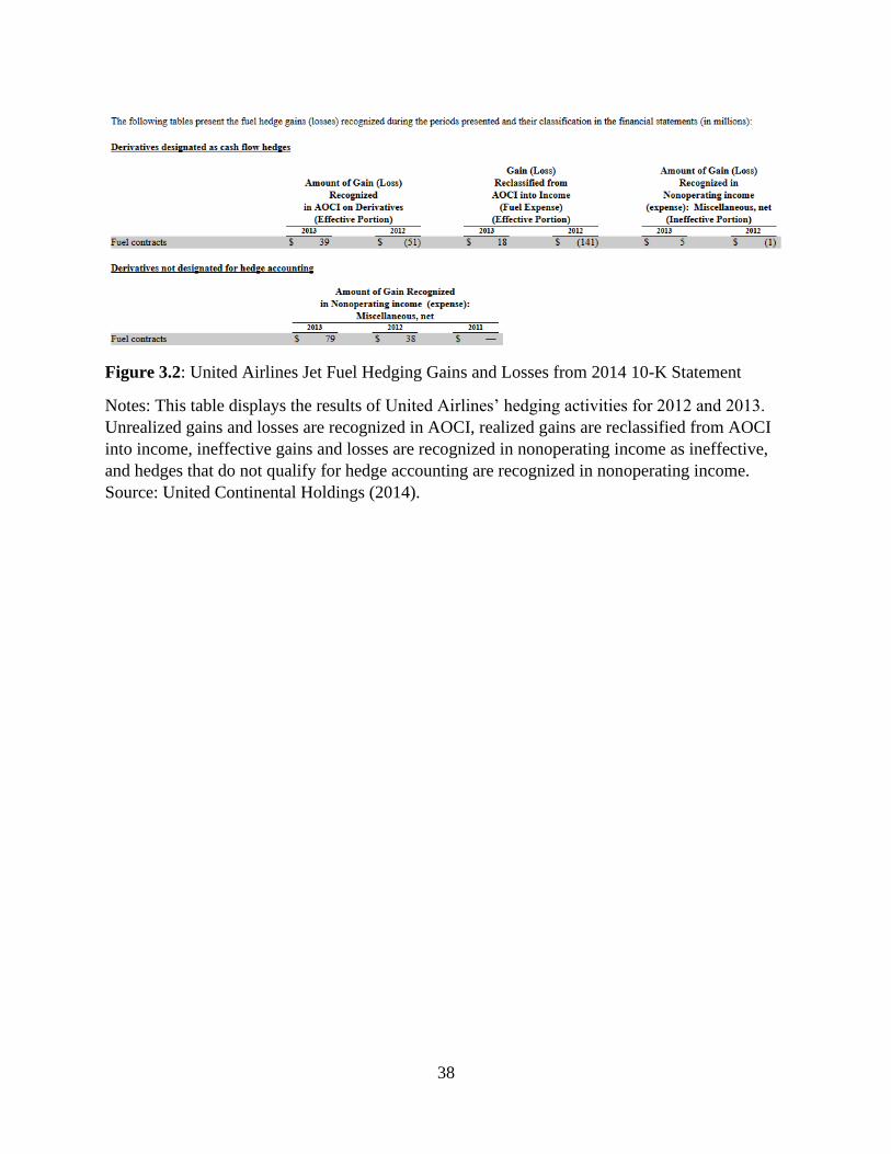
38

Figure 3.2: United Airlines Jet Fuel Hedging Gains and Losses from 2014 10-K Statement

Notes: This table displays the results of United Airlines’ hedging activities for 2012 and 2013.

Unrealized gains and losses are recognized in AOCI, realized gains are reclassified from AOCI

into income, ineffective gains and losses are recognized in nonoperating income as ineffective,

and hedges that do not qualify for hedge accounting are recognized in nonoperating income.

Source: United Continental Holdings (2014).

39

CHAPTER FOUR:

HEDGING GAINS AND LOSSES AND FIRM VALUE

4.1 Background

4.1.1 Justification for Replication

One of the suggestions from Carter et al. (2017) on the future of hedging research is the

reproduction of previous work over different time periods and samples of firms within the same

industry. A prime candidate for replication is the seminal empirical study on jet fuel price

hedging in the airline industry done by Carter, Rogers, and Simkins in 2006 They find a jet fuel

“hedging premium” – an increase in firm value from hedging - of approximately 10.2%.

Additionally, they show that the source of the increased value comes from additional capital

expenditures due to jet fuel hedging. This comports with the theory of Froot, Scharfstein, and

Stein (1993), that hedging allows firms to finance additional investment that they would not be

able to fund otherwise. There are numerous reasons why another analysis of the hedging

premium will improve understanding of hedging by airlines.

The first reason for performing a more recent analysis is that hedging has been a part of

the risk management landscape in the airline industry for a longer period of time. This allows an

investigation into hedging behavior and the hedging premium over different periods of time.

Carter Rogers and Simkins (2006) use a sample of twenty-eight unique airlines over a period

from 1992 to 2003 (this chapter will henceforth refer to the data used by Carter, Rogers, and

40

Simkins (2006) and the 1992 to 2003 time period in their study as the “CRS data” and “CRS

time period,” respectively). During this time, there were no major events that greatly affected

the price of jet fuel, and the only important event that affected the airline industry (the September

11, 2001 terrorist attacks) occurred towards the end of the period.

Since 2003, the price of jet fuel has become significantly more volatile. Over the course

of the CRS time frame, the price of jet fuel varied from 0.3 to 1.05 dollars per gallon with a

standard deviation just over 0.15 dollars per gallon. The largest month-to-month increase in jet

fuel prices was 0.50 dollars per gallon. In the 11 years after, from 2004 to 2014, the high jet fuel

price nearly quadrupled to 3.88 dollars per gallon while never falling below 0.93 dollars per

gallon. The standard deviation of jet fuel prices increased almost by a factor of five to 0.70

dollars per gallon, with a high month-to-month increase of 1.00 dollars per gallons. The

advantage that hedging airlines have over non-hedging airlines may be greater during periods

when changes in jet fuel prices are significantly larger in magnitude than when changes are more

modest.

A second reason for revisiting jet fuel hedging is that airlines are choosing to hedge more

often. In the CRS time period, airlines hedged on average 10.9% of their future jet fuel

requirements (see Carter, Rogers, and Simkins (2006), Table IV on p. 67).15 Airlines hedged a

positive amount of their future jet fuel requirements in 37% of all airline-year observations (p.

67). Between 1995 and 2014 (the time period used in the analysis performed in this

dissertation), the average percentage of jet fuel hedged for all years rose to 14.8%, and 51.4% of

all airline-years had a positive amount of jet fuel hedging. However, the average amount of jet

15 The 10.9% figure includes airline-years in which the amount of jet fuel hedging is zero.

41

fuel hedged in airline-years with a positive amount of hedging has remained relatively constant;

29.4% from 1992 to 2003 (see Carter, Rogers, and Simkins (2006), Footnote 5, p. 59) and 28.8%

from 1995 to 2014. One possible explanation for the increase in hedging is that airlines have an

incentive to hedge jet fuel more often as its price becomes more volatile. Not hedging jet fuel

prices, especially when the magnitude of an unexpected increase in price is greater than before,

will be more costly. As airlines gain experience with hedging and have a greater understanding

of its ability to add value, they will hedge more whenever possible.

A final reason for a new study of jet fuel hedging concerns is the discrepancies in the

theoretical hedging literature on whether financially constrained firms are likely to hedge more

or less. Further empirical study is necessary to determine the correct theory. Froot, Scharfstein,

and Stein (1993) argue that firms more likely to enter financial distress may hedge to reduce the

probability of becoming distress or filing for bankruptcy. On the other hand, Rampini, Sufi, and

Viswanathan (2014) contend the opposite, that financially constrained firms will hedge less

because they do not have the collateral available to purchase hedging contracts. Carter, Rogers,

and Simkins (2006) provide evidence for the latter theory that financial constraint variables have

negative associations with the amount of hedging airlines engage in (although they note the

seeming contradiction between the Froot, Scharfstein, and Stein (1993) framework and their

result).

4.1.2 Study Extension: Hedging Gains and Losses

In the jet fuel hedging literature, hedging has been quantified by the amount of hedging engaged

in by the airline. This is typically measured by the percentage of next year’s expected fuel

requirements that an airline expects to hedge with financial derivatives. The more of its overall

42

jet fuel requirements an airline hedges, the greater the reduction in price risk on its jet fuel

purchases.

However, because jet fuel hedges are costly, the hedge will only provide value if the spot

price of the jet fuel falls within a range where the hedging contract gains value. If an airline has

a call option for a barrel of oil with a strike price of $100 and a premium paid to the seller of the

call option of $10, then the call option will only have a positive value for the airline if the spot

price of jet fuel plus the premium is above $110. Otherwise, the airline will lose value from the

hedge if the spot price of jet fuel remains below that amount. The implicit assumption that is

required to explain how jet fuel hedging provides value to airlines is that the expected value of

its jet fuel hedges is at least zero.

The jet fuel hedging literature does not explicitly take into account the success or failure

of jet fuel hedges in its effect on firm value. A possible reason for this oversight is that gains and

losses data for a firm’s hedging contracts are unreliable before 2001. In June 1998, the Federal

Accounting Standards Board (FASB) issued Statements of Financial Accounting Standards No.

133, Accounting for Derivatives Instruments and Hedging Activities (FAS 133) which required

firms to report the fair value of hedging contracts on their balance sheet. Although firms were

initially required to adopt FAS 133 in the years beginning after June 15, 1999, FASB soon

passed FAS 137 which delayed the implementation of FAS 133 by one year (Southwest, 2001).

Although some airlines did begin reporting on their hedging activities earlier than required, most

airlines did not fully adopt FAS 133 until January 2001.

There are two important types of gains and losses reported on jet fuel hedges that may

influence firm value. Unrealized gains and losses from jet fuel hedges are the changes in the fair

value of the hedges when the spot price of jet fuel changes. These gains and losses do not result

43

in any changes to the cash flow in the airline. They only represent a mark-to-market change in

the value of an unexercised financial derivative. Since unrealized gains and losses describe the

value of an asset, changes in the value of the asset should have a positive relationship with firm

value.

The second significant type of gain and loss from hedging is realized gains and losses.

These gains and losses are a result of exercising a hedging contract to purchase jet fuel. Unlike

their unrealized counterparts, realized gains and losses will affect the airline’s cash flow. If an

airline realizes positive gains on its hedges, then it may be able to use the increased cash flow to

fund investment. Realized gains and losses should have a positive relationship with firm value.

4.2 Jet Fuel Price Exposure

One of the most significant risk exposures that airlines face comes from the volatility of jet fuel

prices. Carter, Rogers, and Simkins (2006) first measure risk exposure from jet fuel prices by

regressing the monthly equally-weighted rate of return for the sample of airlines on the return for

an equally-weighted market portfolio and the percent change of the Gulf Coast jet fuel spot price.

They find a 1% increase in jet fuel prices would correspond to a 0.11% decrease in airline stock

prices. For a one standard deviation increase in the price of jet fuel – a 25% change – the airline

industry’s average monthly stock price would decrease by nearly 2.75% (p. 60).

This analysis is repeated for the current sample of airlines from January 2000 to

December 2014.16 Over this time period, the coefficient on the percent change in jet fuel price

was -0.35, that is, a 1% increase in jet fuel prices would correspond to a 0.35% decrease in

16 The earliest date available for the rate of return variables in the Center for Research in Security Prices (CRSP)

database is January 2000. The airlines chosen for this study come directly from the sample selected by Rampini,

Sufi, and Viswanathan (2014).

44

airline industry stock prices. For a one standard deviation increase in the price of jet fuel – a

48% change in this sample – the average monthly stock price for airlines would decrease by

16.8%. This effect of a one standard deviation change in jet fuel prices is significantly larger in

this study than the result in Carter, Rogers, and Simkins (2006). This is driven by both the

increased sensitivity to airline stock prices and the higher variance in jet fuel prices over the time

frame of this analysis.

4.3 Summary Statistics and Variable Discussion

The summary statistics for the variables used in the reproduction of the Carter, Rogers, and

Simkins (2006) study are provided in Table 4.1. The date range for these variables is 1995 to

2014. Column (6) of the table gives the mean values for the variables from the original analysis

with a date range of 1992 to 2003.

Jet fuel hedging is measured by two variables, the fraction of next year’s jet fuel

requirement hedged and an indicator for a positive fraction of jet fuel hedged. The fraction of

next year’s jet fuel requirements hedged is a continuous variable that describes the amount of jet

fuel hedging that an airline engages in. The jet fuel hedging indicator is a binary variable that is

one if the airline hedges a positive amount of its expected jet fuel requirements for the following

year and zero if the does not hedge any of its jet fuel requirements next year. This variable only

considers the airlines decision to hedge some positive fraction of its future jet fuel requirements.

Compared to the CRS data, airlines are hedging their future jet fuel requirements more often and

hedging a greater amount of their expected jet fuel usage than before.

Firm value is measured by Tobin’s Q. Carter, Rogers, and Simkins (2006) use an

approximation of Tobin’s Q described by Chung and Pruitt (1994). For the data used in this

45

dissertation, the minimum value of the Q ratio is -0.240. Since Tobin’s Q cannot be negative, a

potential remedy for this problem is to translate all values of Tobin’s Q by adding constant, α, to

eliminate any negative values before performing a log transformation. The value of α is chosen

so that the new minimum value is close to the minimum Tobin’s Q from the CRS data. In this

dissertation, a value of α = 0.280 is chosen. The statistics for Tobin’s Q after the adjustment are

shown in Table 4.1.

Firm size, debt capacity, and intensity of investment are provided by the log of total

assets, long-term debt-to-assets, and capital expenditures-to-sales, respectively. Airlines are

larger in size than before, most likely as a result of consolidation of airlines within the industry

due to significant mergers between major carriers. Airlines have greater leverage compared to

the CRS data. The amount of investment by airlines is nearly identical in both studies.

Carter, Rogers, and Simkins (2006) adjust the log of assets, Tobin’s Q, capital

expenditures-to-sales, and long-term debt-to-assets to account for operating leases of aircraft that

do not appear on an airline’s balance sheet. Damodaran (2002) provides a method for this

adjustment by adding the net present value of operating leases to total assets and long-term debt.

Changes in the previous two variables result in a lease-adjusted Tobin’s Q (which remains

translated as described above). Capital expenditures are adjusted by adding the net present value

of operating leases to capital expenditures. After accounting for operating leases, airlines are

still larger and have more leverage on average in this study’s data, although the average level of

investment declined.

46

Financial constraint variables include cash flow-to-sales, cash-to-sales, credit rating, and

Z-score.17 Cash flow-to-sales and cash-to-sales are measures of internal financing for investment

and collateral available to purchase hedging contracts. Although cash flow-to-sales are similar in

the CRS data and the data for this study, airlines have lower cash-to-sales on average in this

study. Credit rating and Z-score provide proxies for the probability of bankruptcy while credit

rating may also be considered as a measure of an airline’s ability to secure external financing.18

The average end of year credit rating is slightly higher (e.g., a lower numerical value) compared

to the CRS data. However, airlines in this study have a greater probability of bankruptcy based

on lower average Z-scores compared to the CRS data.

Tax loss carryforwards-to-assets are a proxy for tax convexity. Airlines that take

advantage of tax loss carryforwards reduce the tax liability for time periods when profits are

positive. This suggests that use of tax loss carryforwards is positively related to the convexity of

a firm’s tax function. This dissertation’s sample of airlines displays a higher use of tax loss

carryforwards than in the CRS study.

Managerial compensations variables consider the number stock and stock option awards

in all executives and CEO compensation packages as a fraction of total shares outstanding for the

airline. Between this study’s data and the CRS sample, executives and CEOs are both receiving

stock and option awards that are a smaller fraction of outstanding shares. This is likely a result

17 Credit ratings are given as numerical values with 2 being the highest credit rating (AAA) and 28 the lowest (D).

Airlines without credit ratings in a given year are given values of 30 to be consistent with Carter, Rogers, and

Simkins (2006). 18 Carter, Rogers, and Simkins (2006) do not explicitly state a yearly measure of credit rating (e.g., mean, median, or

end of year credit ratings). Regressions in this study use end of year credit ratings, although there are no significant

changes in results using any of the yearly constructions for credit rating.

47

of stock and option compensation increases being outpaced by the growth of the airline’s

outstanding stock shares.

The last set of variables account for other forms risk management. Fuel pass-through

agreements and charters operations are two additional ways that an airline can reduce its jet fuel

price risk by passing it on to another airline. Airlines use financial derivatives to hedge against

interest rate and foreign currency risk. Each of these forms of risk management is represented by

a binary variable. The fuel pass-through indicator equals one if the airline has an agreement in

place that transfers the fuel costs to another airline and zero otherwise. The charter indicator is

one if the airline charters some portion of its aircraft to another airline or individual customers

and zero otherwise. In the time period for this analysis, the fraction of airline-years in the

sample where there are fuel pass-through agreements or charter operations have both declined.

The interest rate and foreign currency indicators are one if the airline holds any kind of financial

derivate to hedge against changes in interest rates or foreign currencies, respectively, and zero

otherwise. Airlines are hedging against interest rates slightly less often in this study but hold

derivative instruments for foreign currencies more often compared to the CRS data.

4.4 Determinants of Jet Fuel Hedging

The first major empirical analysis done by Carter, Rogers, and Simkins (2006) is to evaluate the

firm characteristics that influence hedging by airlines. They create a model based on the

theoretical work of Smith and Stulz (1985) and Froot, Scharfstein, and Stein (1993). The most

important factors from these theories that affect airlines’ hedging decisions include financial

constraints, tax convexity, and managerial incentives. Although they are not explicitly discussed

in the general hedging theories, other factors that can affect airlines’ hedging practices are used

as controls in the model. Airlines may employ other methods of managing jet fuel price risk,

48

such as charter operations and fuel pass through agreements, and hedge risk from sources like

interest rates and foreign currencies.

The base model used to determine the effects that these variables have on jet fuel hedging

is described by equation (1) below.

𝐽𝑖𝑡 = 𝛼0 + 𝛽𝐹𝑖𝑡 + 𝛾𝑋𝑖𝑡 + 𝛿𝑀𝑖𝑡 + 𝜃𝐺𝑖𝑡 + 𝑢 (1)

J is the measure of jet fuel hedging by airline i at time t. F represents financial constraint

variables described above. X represents tax convexity measured by tax-loss carryforwards. M

represents managerial incentive variables, and G represents other forms of risk management. u is

the idiosyncratic standard error.

4.4.1 Predicted Effects on Jet Fuel Hedging

In Table 4.2, column (1) shows the expected effects that each of the controls should have on

hedging by airlines as predicted by Rogers, Carter, and Simkins (2006).19 Each of the

explanatory variables in the table is separated into one of four different groups: (A) financial

constraint variables, (B) tax convexity, (C) managerial incentives, and (D) other risk

management strategies. Cells with a plus sign (+) indicate a positive relationship with hedging

where higher values of the explanatory variables correspond to more hedging. Similarly, cells

with a minus sign (-) indicate a negative association with hedging. Higher values correlate to

less hedging.

Columns (2) to (4) of Table 4.2 provide the signs of the results in Table V from Carter,

Rogers, and Simkins (2006, p. 69). Columns (2) and (3) both use the continuous jet fuel hedging

measure as the dependent variable, and column (3) replaces Tobin’s Q, log of assets, capital

19 See pages 66-70 of Carter, Rogers, and Simkins (2006) for a discussion of each variable’s effect on hedging.

49

expenditures-to-sales, and long-term debt-to-assets with their lease-adjusted counterparts.

Column (4) uses the jet fuel hedging indicator as the measure of hedging. In each specification,

the expected signs for each variable largely match with the empirical results, but there are some

notable exceptions within the financial constraints measures.

The initial literature on hedging suggests that more financially constrained firms will

hedge more to lower their expected costs of distress. Carter, Rogers, and Simkins (2006) predict

negative effects financial constraint variables on hedging. Rampini, Sufi, and Viswanathan

(2014), on the other hand, notice that many airlines give financial constraints as a reason not to

hedge. They reason that financially constrained airlines, although they may desire to hedge, are

unable to do so since they are less likely to have the collateral necessary to finance costly

hedging contracts. They would expect a positive relationship between financial constraint

variables and hedging.

The estimates for the expected productivity of investment measures - capital

expenditures-to-sales and Tobin’s Q - generally comport with the Froot, Scharfstein, and Stein

(1993) model. Airlines with higher capital expenditures and firm values will hedge more to

increase internal funds to invest in more profitable projects. The estimates for variables that are

related to financial distress costs, however, mostly follow the Rampini, Sufi, and Viswanathan

(2014) theory. Long-term debt-to-assets and credit rating both show negative relationships with

the amount of jet fuel hedged. Airlines with more debt and worse credit ratings may not be able

to acquire external financing for investment and not have financial collateral to purchase hedging

contracts. Log of assets and cash flow-to-sales have positive relationships with hedging. Larger

airlines will hedge more, possibly as a result of smaller airlines substituting to less costly forms

50

of jet fuel price risk management such as fuel pass through agreements. Airlines with low cash

flow have less ability to buy hedges.

Some variables are omitted from the Carter, Rogers, and Simkins (2006) tests. They drop

any variable that does not have at least weak statistical significance in their estimates (these are

labeled as “dropped” in Table 4.2), although it is unclear the precise statistical threshold they

apply. The thresholds used for this study are discussed in section 4.4.2.1.

4.4.2 Estimated Effects on Jet Fuel Hedging

The same estimation methods that Carter, Rogers, and Simkins (2006) use to determine the

factors most associated with jet fuel hedging are employed for this part of the dissertation. The

first two estimates use the continuous measure of jet fuel hedging as the dependent variable in a

Tobit model. Airlines are not observed increasing their jet fuel price risk by hedging a negative

amount of their jet fuel purchases. The hedging variable will be left censored at zero. The third

regression applies a logit regression with the indicator variable for jet fuel hedging as the

dependent variable.

4.4.2.1 Dropping Statistically Weak Explanatory Variables

As discussed at the end of section 4.4.1, Carter, Rogers, and Simkins (2006) drop any variable

with weak statistical significance. However, they do not give an explicit standard or process to

determine how statistically insignificant a variable must be to remove it from the final results. In

this section, by observing the minimum and maximum p-values for each variable in the three

models used, a reasonable criterion to drop insignificant regressors is developed.

The first observation from Table V in Carter, Rogers, and Simkins (2006, p. 69) is that

two variables, capital expenditure-to-sales and cash-to-sales, are not statistically significant

51

within at least the 10% level in any of the specifications. The minimum p-values for these two

variables are 0.102 and 0.109, respectively, while the maximum p-values are 0.262 and 0.179,

respectively. Although these variables do not meet the threshold for statistical significance at

standard levels, their p-values may be close enough to be included.

Second, the variables that are statistically significant in at least one of the models have p-

values that may vary widely in the others in which the variable is not significant. Long term

debt-to-assets is only statistically significant in Model 2 when it is lease adjusted, but highly

insignificant in Models 1 and 3 with p-values of 0.579 and 0.619, respectively. Tobin’s Q is

significant in Models 1 and 2 but insignificant in Model 3 with a 0.413 p-value. The variables do

not have to be significant or be “close” to significant in each of the models to be included.

Based on these observations, the following process will be used to obtain the final set of

variables in the jet fuel hedging regressions. Each of the variables listed in Table 4.2 are used in

the initial model runs.

1. Estimate the models and drop any regressor in which the p-value for each of the three

specifications is above 0.400.

2. Rerun the estimates without the dropped variables from the previous step. Drop the

regressors from the most current model runs with p-values above 0.400 for all three

models, even if the variable met the threshold from a previous model run.

3. The final set of variables are obtained when all of the remaining regressors have a p-

value below 0.400 for at least one of the three models.

In the initial model run, three variables displayed weak statistical significance with jet fuel

hedging. The jet fuel pass-through agreement indicator (with minimum p-value of 0.998),

52

executive options-to-shares outstanding (0.558), and tax-loss carryforwards-to-asset (0.486) were

dropped from the model. In the second run, an additional three variables were found to be highly

insignificant: log of assets (minimum p-value of 0.465), executive shares-to-shares outstanding

(0.499), and the charter indicator variable (0.454). The third run of the model found no

additional statistically weak variables.

4.4.2.2 Final Estimates

The results for the determinants of jet fuel hedging for this dissertation are shown in Table 4.3.

A comparison of these results to the theories of hedging is discussed first, followed by a

comparison of the estimates from this study and the CRS results.

The variables related to investment opportunities, particularly capital expenditures-to-

sales and Tobin’s Q, have a consistent positive relationship with hedging which matches the

Froot, Scharfstein, and Stein (1993) theoretical framework. Recall that the financial constraint

variables may have multiple interpretations based on the theories of Smith and Stulz (1985) and

Rampini, Sufi, and Viswanathan (2014). The former argued that firms approaching financial

distress will hedge more while the latter realized that firms nearing distress will hedge less or not

at all due to lack of collateral to purchase hedging contracts. The tests conducted in this study

support Rampini, Sufi, and Viswanathan’s (2014) conclusion that financial constraints are

associated with less hedging. Long-term debt-to-assets, end year credit rating, and Z-score all

have negative and highly statistically significant estimates. Cash-to-sales also marginally

supports Rampini, Sufi, and Viswanathan (2014) as cash can be used to hedge. All three

estimates are positive but only in the third model is it statistically significant. Cash flow-to-sales

has a negative relationship with the amount of hedging (the first two models) but a positive

53

association with the decision to hedge (the third model). However, all three estimates have no

statistical relation to hedging.

This study finds little evidence to support the relationship between hedging and tax

convexity or managerial incentives. Tax loss carryforwards-to-assets were dropped from the

final estimates as were executive shares-to-shares outstanding and executive options-to-shares

outstanding. CEO shares-to-shares outstanding and CEO options-to-shares outststanding have

negative and positive relationships, respectively, to hedging which is the opposite of what is

predicted by Smith and Stulz (1993). However, both CEO shares and CEO options-to-shares

outstanding are marginally significant (p-values of 0.083 and 0.121, respectively) in the first

model only and highly insignificant in the other two.

Considering other forms of risk management, charter arrangements and fuel pass-through

agreements had weak statistical associations with jet fuel hedging and were dropped from the

final results. The indicators for interest rate and foreign currency hedges have positive

relationships with jet fuel hedging but the only consistently significant estimates are in the third

model with the decision to hedge jet fuel (the second model estimates are marginally significant

for the interest rate indicator but insignificant for the foreign currency indicator). This suggests

that airlines that hedge in one area of risk are more likely to hedge other risks. Hedging against

interest rates or foreign currencies is unlikely to affect the amount of jet fuel hedging.

The estimates of the determinants of jet fuel hedging in this study are largely consistent

with the Carter, Rogers, and Simkins (2006) results. Both sets of results are consistent with the

Froot, Scharfstein, and Stein (1993) theory on hedging in which firms that are more profitable

(Tobin’s Q) or have more investment opportunities (capital expenditures-to-sales) will hedge

more. The earlier Carter, Rogers, and Simkins (2006) time period finds a higher degree of

54

significance in firm profitability than in investment opportunities while the current time frame

sees investment opportunities as a more statistically significant factor.

For the variables relating to financial constraints, this study’s estimates show a much

higher degree of statistical significance in the financial distress regressors such as long-term

debt-to assets, end year credit rating, and Z-score. Carter, Rogers, and Simkins (2006) found

moderate significance in their credit rating and long-term debt-to-assets estimates while Z-score

was too insignificant to include in the final results. In this study, long-term debt-to-assets and

credit rating are both highly significant while Z-score is still at least moderately significant in all

three models.

Both sets of results find no relation between tax convexity and jet fuel hedging.

Managerial compensation incentives have limited explanatory power in the models. Carter,

Rogers, and Simkins (2006) only find executive sharesholdings-to-shares outstanding to be

significant in their results. This study finds CEO shareholdings-to-shares outstanding to be

statistically significance at any standard level.

4.4.3 Summary of Determinants of Jet Fuel Hedging

Section 4.4 of this study finds further empirical evidence that the Rampini, Sufi, and

Viswanathan (2014) model relating financial constraints and hedging is correct. More

financially constrained airlines, particularly those that are in financial distress or are about to

enter distress, are less likely to hedge in both the amount of jet fuel hedging and in their decision

to hedge or not. The Froot, Scharfstein, and Stein (1993) framework – firms with higher

profitability and more investment opportunities hedge more – is also supported. Similar to

Carter, Rogers, and Simkins (2006), tax convexity and managerial compensation are generally

55

insignificant factors in explaining jet fuel hedging by airlines. Finally, the positive and

statistically significant relationship between the indicator variables for jet fuel, interest rate, and

foreign currency hedges suggests that hedging one type of risk will not crowd out the hedging of

other sources of risk. Airlines will attempt to manage jet fuel are just as likely to hedge interest

rate, and foreign currency risk.

4.5 Effect of Jet Fuel Hedging on Firm Value

The primary motivation in the Carter, Rogers, and Simkins (2006) study is to analyze how jet

fuel hedging by airlines affects the value of the firm. They measure this effect by determining a

“hedging premium” – the increase in firm value for an airline that hedges an average amount of

its jet fuel requirements compared to an airline that does not hedge any of its fuel requirements.

The nature of the hedging premium is investigated in multiple ways. First, the size of the

premium is calculated using multiple estimation methods and hedging measures. Second,

additional specifications are tested to account for endogeneity issues between hedging and firm

value. The final major test they perform is to establish capital expenditures as the source of the

hedging premium in one-stage and two-stage regressions. In each case, a discussion of this

study’s results is compared to the CRS findings.

4.5.1 Firm Value Models and Specifications

The control variables used in the firm value models of Carter, Rogers, and Simkins (2006)

follow closely with the firm value models in Allayannis and Weston (2001). These variables

include measures of firm size (log of assets), access to financial markets (indicator for dividends

paid), leverage (long-term debt-to-assets), profitability (cash flow-to-sales), investment growth

(capital expenditures-to-sales and advertising-to-sales), credit rating, and a set of year

56

dummies.20 Other variables that Carter, Rogers, and Simkins (2006) use in the models that

Allayannis and Weston (2001) do not include cash-to-sales and indicators for other forms of risk

management such as fuel passthrough agreements, charter operations, and usage of interest rate

derivatives and foreign currency derivatives. The jet fuel hedging measures, both the indicator

for a positive amount of jet fuel hedged and the percentage of jet fuel hedged the following year,

are the variables of interest.

Carter, Rogers, and Simkins (2006) estimate the model using three estimation methods:

pooled ordinary least squares (pooled OLS), fixed effects, and feasible generalized least squares

(FGLS). No justification is provided for the fixed effects and FGLS techniques other than as a

robustness check on the size and significance of the hedging premium. The indicator for a

positive amount of jet fuel hedging is only estimated using pooled OLS. The continuous jet fuel

hedging variable is tested using all three estimation procedures.

The model is described by equation (2).

𝑉𝑖𝑡 = 𝛼0 + 𝛽𝐽𝑖𝑡 + 𝛾𝑋𝑖𝑡 + 𝑢𝑖𝑡 (2)

where V is the value of airline i at time t. J is the measure of jet fuel hedging and X represents

the remaining controls. u is the idiosyncratic standard error.

4.5.2 Size of the Hedging Premium

In this study, the same model construction and estimation procedures are followed as described

in section 4.5.1. Table 4.4 shows the results of the estimates of jet fuel hedging on firm value

described in equation (2). Column (1) displays the pooled OLS estimate for the jet fuel hedge

20 See section 2.1 of Allayannis and Weston (2001, p. 251-254) for a brief discussion to justify the inclusion of these

variables.

57

indicator. Columns (2), (3), and (4) show the results for the continuous jet fuel hedging variable

using pooled OLS, fixed effects, and FGLS, respectively.

The estimates for this study and in Carter, Rogers, and Simkins (2006) are similar. The

coefficient of the indicator for positive jet fuel hedging is statistically insignificant in both

results. There is no empirical evidence to suggest that an airline’s decision to hedge a positive

amount of its fuel requirements has any statistical effect on value. However, using the fraction

of next year’s jet fuel requirements hedged as the measure of hedging, the tests show positive

and statistically significant relationships with firm value over all three estimation methods. For

the pooled OLS estimate, the average increase in value for each percent of next year’s jet fuel

requirements hedged is 0.241%. Including only airline-year observations with a positive amount

of jet fuel hedging, airlines hedged on average 28.8% of next year’s fuel requirements. An

airline that hedges the average amount of its future jet fuel requirements over this study’s time

period can expect an average increase in value of 6.94%. This hedging premium is somewhat

smaller than the 10.2% premium found by Carter, Rogers, and Simkins (2006, p. 73). The

difference between the hedging premiums comes from the greater effect that each percent of jet

fuel hedged adds to value (0.348%) in the CRS data.

The hedging premium found in this study is more robust in the fixed effects and FGLS

estimates. The effect that jet fuel hedging has on firm value is only statistically significant using

the FGLS estimation procedure in Carter, Rogers, and Simkins (2006) and not significant at any

standard level when accounting for airline fixed effects. In this analysis, the coefficients are

significant in both fixed effects and FGLS estimates. However, the hedging premium remains

smaller in magnitude over all estimates compared to the CRS results.

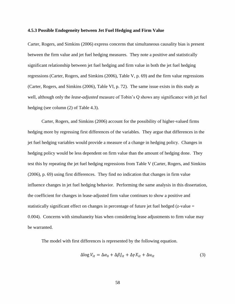
58

4.5.3 Possible Endogeneity between Jet Fuel Hedging and Firm Value

Carter, Rogers, and Simkins (2006) express concerns that simultaneous causality bias is present

between the firm value and jet fuel hedging measures. They note a positive and statistically

significant relationship between jet fuel hedging and firm value in both the jet fuel hedging

regressions (Carter, Rogers, and Simkins (2006), Table V, p. 69) and the firm value regressions

(Carter, Rogers, and Simkins (2006), Table VI, p. 72). The same issue exists in this study as

well, although only the lease-adjusted measure of Tobin’s Q shows any significance with jet fuel

hedging (see column (2) of Table 4.3).

Carter, Rogers, and Simkins (2006) account for the possibility of higher-valued firms

hedging more by regressing first differences of the variables. They argue that differences in the

jet fuel hedging variables would provide a measure of a change in hedging policy. Changes in

hedging policy would be less dependent on firm value than the amount of hedging done. They

test this by repeating the jet fuel hedging regressions from Table V (Carter, Rogers, and Simkins

(2006), p. 69) using first differences. They find no indication that changes in firm value

influence changes in jet fuel hedging behavior. Performing the same analysis in this dissertation,

the coefficient for changes in lease-adjusted firm value continues to show a positive and

statistically significant effect on changes in percentage of future jet fuel hedged (z-value =

0.004). Concerns with simultaneity bias when considering lease adjustments to firm value may

be warranted.

The model with first differences is represented by the following equation.

∆log 𝑉𝑖𝑡 = ∆𝛼0 + ∆𝛽𝐽𝑖𝑡 + ∆𝛾𝑋𝑖𝑡 + ∆𝑢𝑖𝑡 (3)

59

where V is the value of airline i at time t. J is the measure of jet fuel hedging and X represents

the remaining controls. u is the idiosyncratic standard error. Table 4.5 shows the results for the

firm value regressions for equation (3). Changes in airlines’ decisions to hedge or not shows no

statistically significant relationship with changes in firm value as shown in column (1), unlike

the positive and significant result found by Carter, Rogers, and Simkins (2006). In column (2),

changes in the amount of jet fuel hedged shows a large positive and highly significant effect on

changes in value. The expected hedging premium for an airline that changes its percentage of

future fuel purchases hedged by the sample average for positive jet fuel hedging years is 10.45%,

which is approximately fifty percent larger than the 6.94% premium found in Table 4.4. Carter,

Roger, and Simkins (2006) on the other hand, find that the hedging premium decreases from

10.2% in the original firm value regressions (Table VI, p. 72) to 5.5% in the first difference firm

value regressions (Table VII, p. 75).

4.5.4 Hedging Premium through Capital Expenditures

Carter, Rogers, and Simkins (2006) further theorize that the source of the hedging premium

comes primarily from capital expenditures. That is, airlines that hedge are more likely to have

additional cash flow necessary to fund investment. They test this hypothesis in two separate

ways. First, an interaction term between capital expenditures-to-sales and the jet fuel hedging

variables is added to the regressions, and the hedging premium is evaluated. Second, they

perform a two-stage regression in which next year’s capital expenditures are predicted by the

amount of jet fuel hedging done, then using those predicted values of capital expenditures in the

firm value regressions.

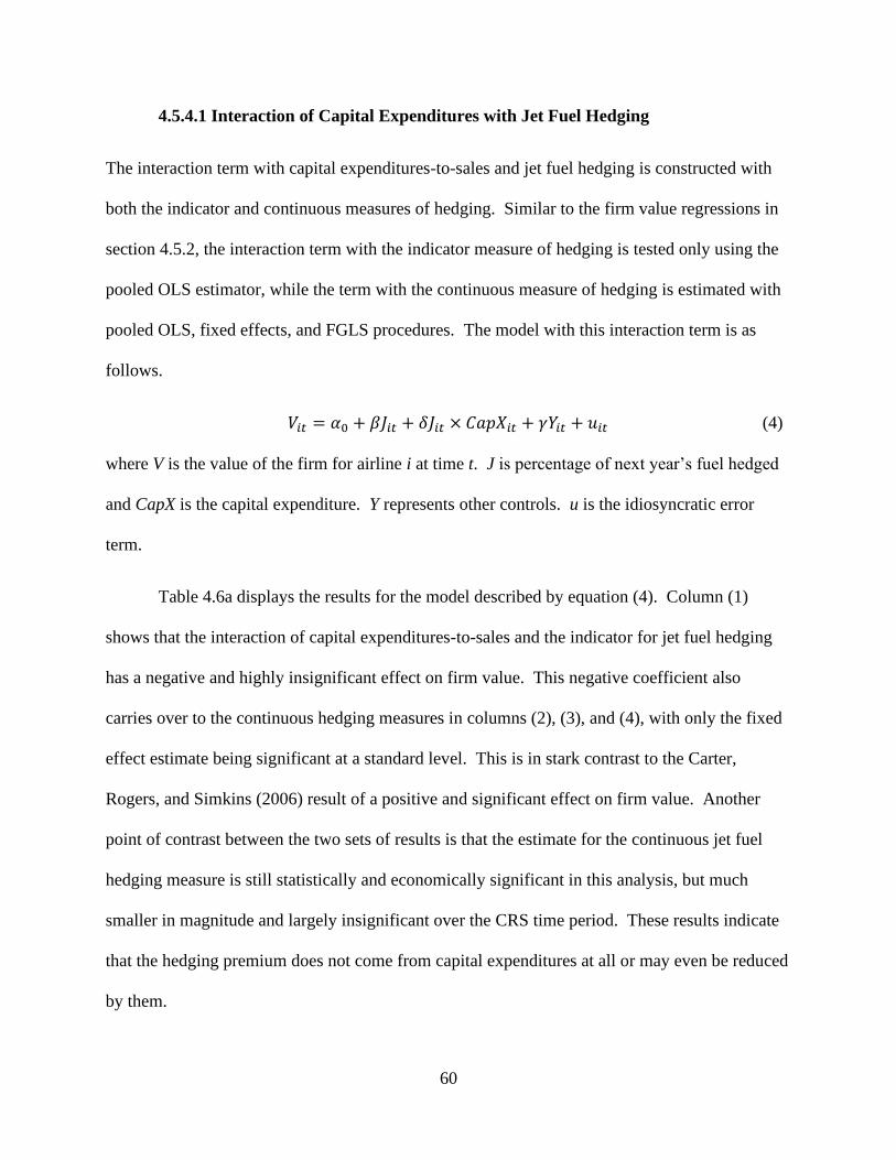
60

4.5.4.1 Interaction of Capital Expenditures with Jet Fuel Hedging

The interaction term with capital expenditures-to-sales and jet fuel hedging is constructed with

both the indicator and continuous measures of hedging. Similar to the firm value regressions in

section 4.5.2, the interaction term with the indicator measure of hedging is tested only using the

pooled OLS estimator, while the term with the continuous measure of hedging is estimated with

pooled OLS, fixed effects, and FGLS procedures. The model with this interaction term is as

follows.

𝑉𝑖𝑡 = 𝛼0 + 𝛽𝐽𝑖𝑡 + 𝛿𝐽𝑖𝑡 × 𝐶𝑎𝑝𝑋𝑖𝑡 + 𝛾𝑌𝑖𝑡 + 𝑢𝑖𝑡 (4)

where V is the value of the firm for airline i at time t. J is percentage of next year’s fuel hedged

and CapX is the capital expenditure. Y represents other controls. u is the idiosyncratic error

term.

Table 4.6a displays the results for the model described by equation (4). Column (1)

shows that the interaction of capital expenditures-to-sales and the indicator for jet fuel hedging

has a negative and highly insignificant effect on firm value. This negative coefficient also

carries over to the continuous hedging measures in columns (2), (3), and (4), with only the fixed

effect estimate being significant at a standard level. This is in stark contrast to the Carter,

Rogers, and Simkins (2006) result of a positive and significant effect on firm value. Another

point of contrast between the two sets of results is that the estimate for the continuous jet fuel

hedging measure is still statistically and economically significant in this analysis, but much

smaller in magnitude and largely insignificant over the CRS time period. These results indicate

that the hedging premium does not come from capital expenditures at all or may even be reduced

by them.

61

Carter, Rogers, and Simkins (2006) evaluate the total hedging premium in the model by

adding together the portion of the premium that comes from capital expenditures and the portion

that comes from all other sources.21 They find the hedging premium to be between 7.2% and

7.8%, with 38% to 86% of the total hedging premium coming from capital expenditures. A

similar analysis is performed for each of the estimates from Table 4.6. Using the pooled OLS,

fixed effects, and FGLS estimates, the hedging premium evaluates to 7.26%, 8.85%, and 7.74%,

respectively, and capital expenditures reduces the total premium by 1.32%, 5.78%, and 1.33%,

respectively. Although capital expenditures have a negative effect on the hedging premium, the

overall range of the premium remains similar to the premiums of the CRS data.

A major issue with the above analysis is that it does not account for leases. As leases can

make up a large portion of an airline’s capital expenditures, it is important to examine the

interaction of jet fuel hedging and capital expenditures when considering lease adjustments.

Table 4.6b displays the estimates for the model using lease-adjusted variables. Each of the

coefficients for the interaction terms between jet fuel hedging and capital expenditures becomes

positive and statistically significant in each of the three estimation methods. This suggests that

hedging airlines are able to increase firm value through capital expenditures primarily by

investing in additional leased aircraft. The hedging premium is calculated in the same way as

described in footnote 6, except that the average level of capital expenditures becomes 18% after

lease adjustments. The value of the hedging premium in the lease-adjusted estimates is generally

lower than the non-lease-adjusted estimates: 5.8% for the pooled OLS estimate, 8.42% with

21 The portion of the hedging premium that comes from capital expenditures is calculated by multiplying the

coefficient of the interaction term between jet fuel hedging and capital expenditures-to-sales with the average

percentage of future jet fuel requirements hedged over positive hedging airline-years (28.8%) and the average level

of capital expenditures-to-sales over the sample (11.6%). The remaining portion of the premium is calculated by

multiplying the coefficient of the individual jet fuel hedging term with the average percentage of future jet fuel

requirements hedged over positive hedging airline-years.

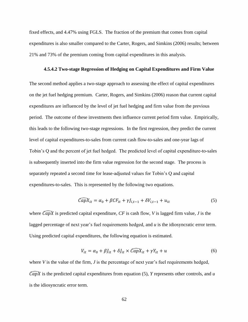
62

fixed effects, and 4.47% using FGLS. The fraction of the premium that comes from capital

expenditures is also smaller compared to the Carter, Rogers, and Simkins (2006) results; between

21% and 73% of the premium coming from capital expenditures in this analysis.

4.5.4.2 Two-stage Regression of Hedging on Capital Expenditures and Firm Value

The second method applies a two-stage approach to assessing the effect of capital expenditures

on the jet fuel hedging premium. Carter, Rogers, and Simkins (2006) reason that current capital

expenditures are influenced by the level of jet fuel hedging and firm value from the previous

period. The outcome of these investments then influence current period firm value. Empirically,

this leads to the following two-stage regressions. In the first regression, they predict the current

level of capital expenditures-to-sales from current cash flow-to-sales and one-year lags of

Tobin’s Q and the percent of jet fuel hedged. The predicted level of capital expenditure-to-sales

is subsequently inserted into the firm value regression for the second stage. The process is

separately repeated a second time for lease-adjusted values for Tobin’s Q and capital

expenditures-to-sales. This is represented by the following two equations.

𝐶𝑎𝑝�̂�𝑖𝑡 = 𝛼0 + 𝛽𝐶𝐹𝑖𝑡 + 𝛾𝐽𝑖,𝑡−1 + 𝛿𝑉𝑖,𝑡−1 + 𝑢𝑖𝑡 (5)

where 𝐶𝑎𝑝�̂� is predicted capital expenditure, CF is cash flow, V is lagged firm value, J is the

lagged percentage of next year’s fuel requirements hedged, and u is the idiosyncratic error term.

Using predicted capital expenditures, the following equation is estimated.

𝑉𝑖𝑡 = 𝛼0 + 𝛽𝐽𝑖𝑡 + 𝛿𝐽𝑖𝑡 × 𝐶𝑎𝑝�̂�𝑖𝑡 + 𝛾𝑌𝑖𝑡 + 𝑢 (6)

where V is the value of the firm, J is the percentage of next year’s fuel requirements hedged,

𝐶𝑎𝑝�̂� is the predicted capital expenditures from equation (5), Y represents other controls, and u

is the idiosyncratic error term.

63

The results of the two-stage estimation procedure are shown in Table 4.7. Columns (1)

and (2) show the first-stage and second-stage estimates, respectively, for the standard measure of

Tobin’s Q and capital expenditures-to-sales, while columns (3) and (4) show the first-stage and

second-stage estimates, respectively, for the lease-adjusted measures of Tobin’s Q and capital

expenditures-to-sales. Using the standard measure of Tobin’s Q and capital expenditures-to-

sales, the signs for the coefficients for the jet fuel hedging and the predicted capital expenditures-

to-sales variables are both positive, however, the estimate for the predicted capital expenditures-

to-sales is statistically insignificant. Considering the lease-adjusted measures for Tobin’s Q and

capital expenditures-to-sales, the predicted capital expenditures-to-sales coefficient is

statistically significant at the 1% level. This provides further evidence that leases are an

important factor in capital expenditures’ effect on the hedging premium.

The hedging premium for the two-stage model is calculated in a similar fashion to the

premium in section 4.5.4.1.22 Carter, Rogers, and Simkins (2006) find a hedging premium of

20.7% in the non-lease-adjusted estimate and a 6.1% premium from the lease-adjusted

regressions. Capital expenditures is responsible for 100% of the former premium but only 65.5%

of the latter premium. In this study, the non-lease-adjusted and lease-adjusted premiums are

11.7% and 3.98%, respectively, with capital expenditures responsible for 56.7% and 76.3% of

the total premium, respectively.

22 For this model, the portion that comes from capital expenditures is found by multiplying the coefficient of the

lagged jet fuel hedging term in the first-stage regression with the predicted capital expenditures-to-sales coefficient

in the second-stage regression and the average percentage of jet fuel hedged for positive hedging airline-years. The

remaining portion of the premium comes from the product of the jet fuel hedging coefficient in the second-stage

regression and the average percentage of jet fuel hedged for positive hedging airline-years.

64

4.5.5 Hedging Premium over Time

The final tests that Carter, Rogers, and Simkins (2006) perform seek to evaluate how the hedging

premium may change over time, different fuel price regimes, and periods with credit rating

upgrades and downgrades. Jet fuel hedging may be more valuable during periods of high

volatility compared to low volatility or when external financing may be more difficult to obtain

during periods of higher financial constraints. The hedging effects are estimated with

interactions between regime dummies and the percent of jet fuel hedged variable using the same

model construction from Table VI (Carter, Rogers, and Simkins (2006), p. 72). They

consistently find the largest hedging premiums during the 2000-to-2003 time frame. During this

period of the sample, prices were the most volatile and airlines experienced a larger number of

downgrades in credit rating.

Hedging effects by year for this study are estimated with the same model described

above. Table 4.8 shows the yearly hedging coefficients for each year from 1996 to 2014. The

years that have positive and statistically significant coefficients in any of the three estimation

methods are 2000, 2003, 2008, and 2011-2012. With the exception of 2003, these years

generally correspond to times in which jet fuel prices reached a local maximum after rising for

one to two prior years with increasing jet fuel prices. This suggests a hedging premium that is

larger during times of high volatility. The only observed negative and statistically significant

coefficient is for 2009 when jet fuel prices plummeted at the height of the severe financial crisis

that began one year earlier in 2008. The most significant effects on the hedging premium

occurred when jet fuel prices were more volatile and less significant when prices were relatively

stable.

65

4.6 Jet Fuel Hedging Gains and Losses and Firm Value

Carter, Rogers, and Simkins (2006) conclude their study by noting that the act of hedging alone

does not always increase firm value. Jet fuel hedging is more likely to have a positive effect on

value when airlines choose an optimal hedging ratio (the fraction of future fuel requirements

hedged) that takes advantage of productive investment opportunities when they are available or a

general reduction in jet fuel expenditures. Furthermore, airlines only accrue cash flow benefits

from hedging when at least some of their hedges have positive value. Thus, airlines that are

more successful with their hedges will accumulate greater cash flow than if they were

unsuccessful or did not hedge at all. Airline that enjoy large gains from hedges or have

successive years of positive gains consequentially have greater incentives to undertake profit-

enhancing investments.

In all previous analyses of jet fuel hedging, airlines are assumed to choose optimal

hedging ratios and the jet fuel hedges used by airlines have at least zero expected value. This

dissertation extends the literature on jet fuel hedging by considering the success or failure of the

hedges. In this section, gains and losses from jet fuel hedges are introduced into the firm value

models in two ways. First, jet fuel hedging gains and losses are directly inserted into the firm

value regressions. Recall from Chapter 3 that hedging gains and losses are separated into four

categories: realized, unrealized, ineffective, and no-hedge accounting gains and losses. The

regressions control for realized gains and losses from jet fuel hedges because it is the only type

of hedging gain or loss that has an effect on the cash flows of the airline. Realized gains and

losses are expected to have a positive relationship with firm value.

Another set of regressions is performed using an interaction term between a realized

hedging gains and losses indicator and the fraction of next year’s jet fuel requirements hedged.

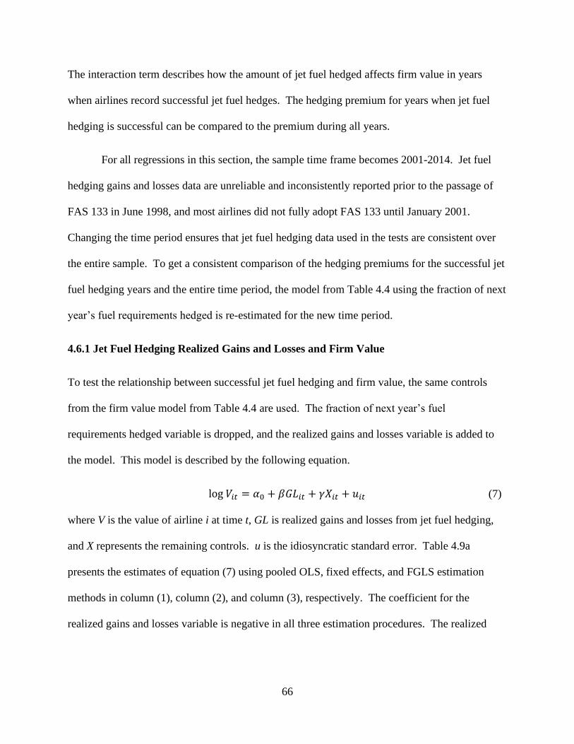
66

The interaction term describes how the amount of jet fuel hedged affects firm value in years

when airlines record successful jet fuel hedges. The hedging premium for years when jet fuel

hedging is successful can be compared to the premium during all years.

For all regressions in this section, the sample time frame becomes 2001-2014. Jet fuel

hedging gains and losses data are unreliable and inconsistently reported prior to the passage of

FAS 133 in June 1998, and most airlines did not fully adopt FAS 133 until January 2001.

Changing the time period ensures that jet fuel hedging data used in the tests are consistent over

the entire sample. To get a consistent comparison of the hedging premiums for the successful jet

fuel hedging years and the entire time period, the model from Table 4.4 using the fraction of next

year’s fuel requirements hedged is re-estimated for the new time period.

4.6.1 Jet Fuel Hedging Realized Gains and Losses and Firm Value

To test the relationship between successful jet fuel hedging and firm value, the same controls

from the firm value model from Table 4.4 are used. The fraction of next year’s fuel

requirements hedged variable is dropped, and the realized gains and losses variable is added to

the model. This model is described by the following equation.

log 𝑉𝑖𝑡 = 𝛼0 + 𝛽𝐺𝐿𝑖𝑡 + 𝛾𝑋𝑖𝑡 + 𝑢𝑖𝑡 (7)

where V is the value of airline i at time t, GL is realized gains and losses from jet fuel hedging,

and X represents the remaining controls. u is the idiosyncratic standard error. Table 4.9a

presents the estimates of equation (7) using pooled OLS, fixed effects, and FGLS estimation

methods in column (1), column (2), and column (3), respectively. The coefficient for the

realized gains and losses variable is negative in all three estimation procedures. The realized

67

gains and losses coefficient is statistically significant at the 5% level in the pooled OLS estimate

but statistically insignificant in the fixed effects and FGLS estimates.

Why is the sign of the coefficient on the jet fuel hedging gains and losses variable

negative when the expected relationship is positive? This counterintuitive result is investigated

in multiple ways. First, a comparison of Table 4.6a and Table 4.6b shows that leases influence

the hedging premium. In untabulated results, when lease-adjusted variables for firm value and

other controls are used, the realized gains and losses coefficient becomes statistically

insignificant for all estimates but remains negative.

Second, outliers in the realized gains and losses variable may influence its relationship

with firm value. Figure 4.1 shows a box plot of non-zero realized gains and losses from jet fuel

hedging. The box plot is constructed in the standard way, with the whiskers extending 1.5 times

the interquartile range from the first and third quartiles.23 Data points outside these whiskers

constitute outliers. Of the eleven outliers that are negative, eight of these are from the years

2009 and 2010 when jet fuel prices fell considerably and all hedging firms suffered large losses.

Five of the nine outliers that are positive come during Southwest’s run of extraordinary hedging

success from 2004 to 2008 which no other airline was able to produce. Eliminating these

outliers from the model estimates may give a more reasonable look at the relationship between

jet fuel hedging gains and losses and the value of the firm.

Table 4.9b shows the results of the estimation of equation (7) after removing outliers

from the sample. Although none of the estimates are statistically significant, all the coefficients

23 The first and third quartiles are -7 and 79, respectively, implying an interquartile range of 86. Applying the

interquartile rule, the ends of the left whisker and right whisker are -136 (-7 – 1.5 × 86) and 208 (79 + 1.5 × 86),

respectively.

68

show a positive relationship with firm value. In untabulated results, using lease-adjusted

variables, the coefficients remain positive and statistically insignificant. The method for

identifying outliers is adjusted by increasing the range of the whiskers of the box plot to 2 times

and 3 times the interquartile range. Estimating the model after eliminating outliers that are

outside 2 times the interquartile range still gives a positive coefficient on realized gains and

losses from jet fuel hedging. However, the coefficient becomes negative and statistically

insignificant after raising the outlier identification threshold to 3 times the interquartile range.

The negative coefficient on realized gains and losses found in Table 4.9a is most likely driven by

the significant losses airlines suffered during the recession that began in 2009.

4.6.2 Measurement of the Hedging Premium for Successful Jet Fuel Hedging

Recall that the hedging premium for jet fuel describes the increase in firm value that an airline

will experience when it hedges an average amount of its jet fuel requirements for the following

year compared to an airline that does not hedge at all. This hedging premium is almost certainly

influenced by the success or failure of its jet fuel hedges. If two airlines hedge the same fraction

of their future jet fuel requirements, the airline that is more successful in its hedging activities

will have more cash flow to fund investment compared to an airline that has less successful

hedges. The estimation results from the previous section show that successful hedging is

associated with lower firm values. Therefore, the hedging premium may be smaller during years

of successful jet fuel hedging.

The firm value model from Table 4.4 is adjusted to add an interaction term between the

fraction of next year’s jet fuel requirements hedged and an indicator for jet fuel hedging realized

gains (i.e., the indicator variable is one when realized gains and losses variable is positive, zero

otherwise) in the current year. Table 4.10 shows the results of these regressions. The

69

coefficients on both the jet fuel hedging variable and the interaction term between hedging and

positive gains indicator is positive and statistically insignificant at standard levels. The hedging

premium for during years in which hedging is successful is approximately 5.6% in pooled OLS

estimate and 7.2% in the FGLS estimate.24 In untabulated results, the jet fuel hedging coefficient

for the original firm value model (Table 4.4) using the adjusted time frame is 0.312 and 0.371 in

the pooled OLS and FGLS estimates, respectively. These hedging coefficients imply a hedging

premium of 9.2% and 10.9%, respectively. The hedging premium when jet fuel hedging gains

and losses are positive is approximately 3% to 4% smaller than the hedging premium over the

entire adjusted time frame.

4.7 Conclusion

Carter, Rogers, and Simkins (2006) is one of the seminal papers on the empirical study of

hedging. They establish that the airline industry is a most suitable environment to study hedging

because of airlines’ exposure to jet fuel price risk and its ideal investment setting matches the

leading theories on hedging and firm value. They determine that the hedging premium for

airlines that hedge jet fuel versus those that do not falls in a range between 5% and 10%.

Furthermore, they also show that a large portion, between 65% and 86%, of the hedging

premium comes from capital expenditures.

In this chapter, a reproduction of the Carter, Rogers, and Simkins (2006) hedging models

is performed using a more recent dataset over a time ranging from 1995 to 2014. Evidence is

found that verifies the Rampini, Sufi, and Viswanathan (2014) model on the determinants of jet

24 Jet fuel hedging gains are positive in 36.8% of all observations and the average jet fuel requirements hedged is

16.2%. The hedging premium is calculated to be (0.141×0.294 + 0.136×0.368×0.294) = 0.031 and (0.172×0.294 +

0.194×0.368×0.294) = 0.039 for the pooled OLS and FGLS estimates, respectively.

70

fuel hedging; that is, more financially constrained firms hedge less rather than more because they

do not have the collateral necessary to purchase costly hedging contracts. The hedging premium

in this empirical analysis is found to be 6.9%, 3.3% smaller than the hedging premium found by

Carter, Rogers, and Simkins (2006). This study additionally finds a negative association

between firm value and the interaction of capital expenditures and hedging, however, this

relationship becomes positive when accounting for lease adjustments in both the one-stage and

two-stage regression models. This suggests that leasing aircraft is important to an airline’s

overall capital expenditures and its effect on firm value.

This chapter contributes to the economic literature on hedging by introducing jet fuel

hedging gains and losses into the firm value models, rather than simply relying on the fraction of

total jet fuel requirements hedged as has been done in previous studies. Successful jet fuel

hedging is shown to have a negative relationship on firm value. This counterintuitive result may

be explained by the significant losses suffered by airlines during the recession in 2009.

Eliminating outliers from the sample using the interquartile rule with a standard box plot results

in a positive relationship between firm value and realized gains and losses. This chapter

continues to find a smaller, but still positive and statistically significant, hedging premium.

Hedging airlines have higher values compared to airlines that do not hedge jet fuel at all.

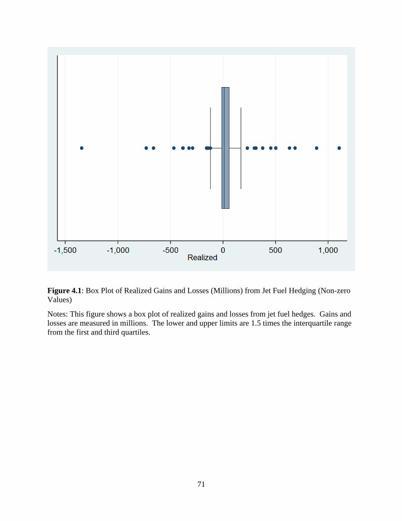
71

Figure 4.1: Box Plot of Realized Gains and Losses (Millions) from Jet Fuel Hedging (Non-zero

Values)

Notes: This figure shows a box plot of realized gains and losses from jet fuel hedges. Gains and

losses are measured in millions. The lower and upper limits are 1.5 times the interquartile range

from the first and third quartiles.

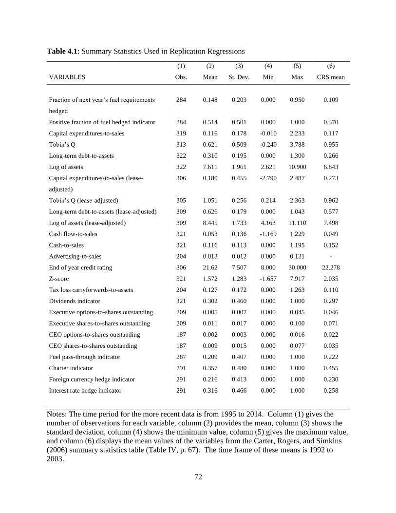
72

Table 4.1: Summary Statistics Used in Replication Regressions

(1) (2) (3) (4) (5) (6)

VARIABLES Obs. Mean St. Dev. Min Max CRS mean

Fraction of next year’s fuel requirements

hedged

284 0.148 0.203 0.000 0.950 0.109

Positive fraction of fuel hedged indicator 284 0.514 0.501 0.000 1.000 0.370

Capital expenditures-to-sales 319 0.116 0.178 -0.010 2.233 0.117

Tobin’s Q 313 0.621 0.509 -0.240 3.788 0.955

Long-term debt-to-assets 322 0.310 0.195 0.000 1.300 0.266

Log of assets 322 7.611 1.961 2.621 10.900 6.843

Capital expenditures-to-sales (lease-

adjusted)

306 0.180 0.455 -2.790 2.487 0.273

Tobin’s Q (lease-adjusted) 305 1.051 0.256 0.214 2.363 0.962

Long-term debt-to-assets (lease-adjusted) 309 0.626 0.179 0.000 1.043 0.577

Log of assets (lease-adjusted) 309 8.445 1.733 4.163 11.110 7.498

Cash flow-to-sales 321 0.053 0.136 -1.169 1.229 0.049

Cash-to-sales 321 0.116 0.113 0.000 1.195 0.152

Advertising-to-sales 204 0.013 0.012 0.000 0.121 -

End of year credit rating 306 21.62 7.507 8.000 30.000 22.278

Z-score 321 1.572 1.283 -1.657 7.917 2.035

Tax loss carryforwards-to-assets 204 0.127 0.172 0.000 1.263 0.110

Dividends indicator 321 0.302 0.460 0.000 1.000 0.297

Executive options-to-shares outstanding 209 0.005 0.007 0.000 0.045 0.046

Executive shares-to-shares outstanding 209 0.011 0.017 0.000 0.100 0.071

CEO options-to-shares outstanding 187 0.002 0.003 0.000 0.016 0.022

CEO shares-to-shares outstanding 187 0.009 0.015 0.000 0.077 0.035

Fuel pass-through indicator 287 0.209 0.407 0.000 1.000 0.222

Charter indicator 291 0.357 0.480 0.000 1.000 0.455

Foreign currency hedge indicator 291 0.216 0.413 0.000 1.000 0.230

Interest rate hedge indicator 291 0.316 0.466 0.000 1.000 0.258

Notes: The time period for the more recent data is from 1995 to 2014. Column (1) gives the

number of observations for each variable, column (2) provides the mean, column (3) shows the

standard deviation, column (4) shows the minimum value, column (5) gives the maximum value,

and column (6) displays the mean values of the variables from the Carter, Rogers, and Simkins

(2006) summary statistics table (Table IV, p. 67). The time frame of these means is 1992 to

2003.

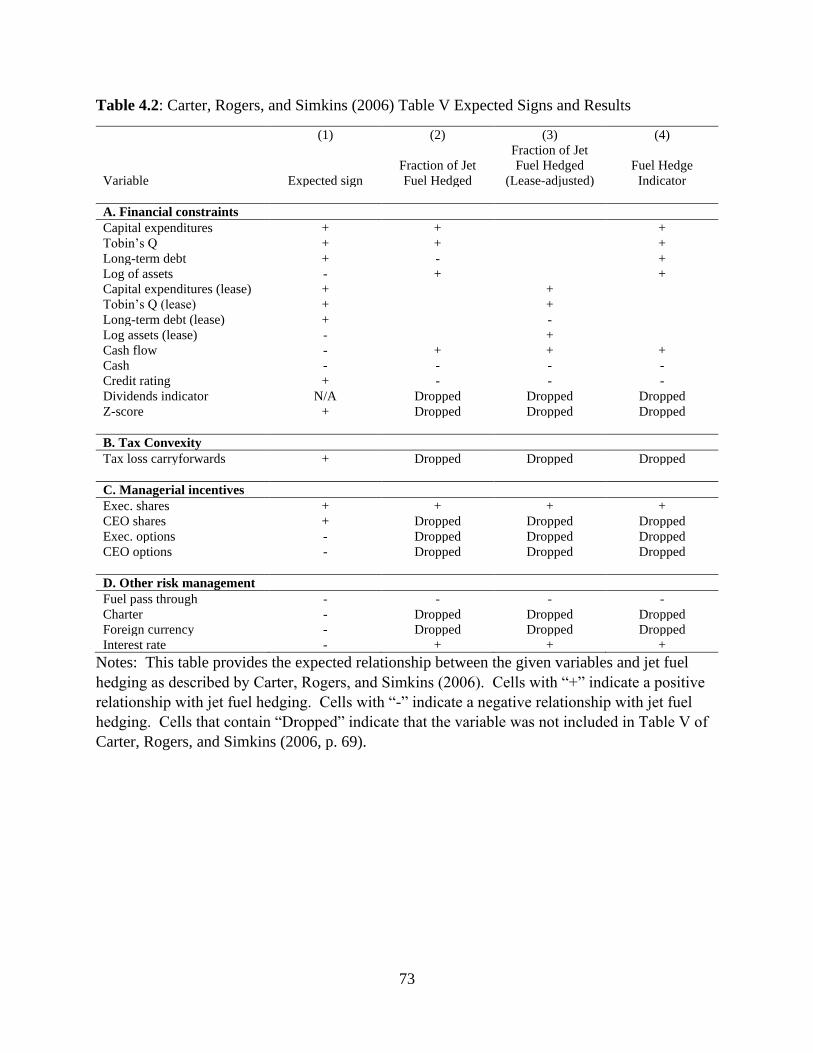
73

Table 4.2: Carter, Rogers, and Simkins (2006) Table V Expected Signs and Results

(1) (2) (3) (4)

Variable Expected sign

Fraction of Jet

Fuel Hedged

Fraction of Jet

Fuel Hedged

(Lease-adjusted)

Fuel Hedge

Indicator

A. Financial constraints

Capital expenditures + + +

Tobin’s Q + + +

Long-term debt + - +

Log of assets - + +

Capital expenditures (lease) + +

Tobin’s Q (lease) + +

Long-term debt (lease) + -

Log assets (lease) - +

Cash flow - + + +

Cash - - - -

Credit rating + - - -

Dividends indicator N/A Dropped Dropped Dropped

Z-score + Dropped Dropped Dropped

B. Tax Convexity

Tax loss carryforwards + Dropped Dropped Dropped

C. Managerial incentives

Exec. shares + + + +

CEO shares + Dropped Dropped Dropped

Exec. options - Dropped Dropped Dropped

CEO options - Dropped Dropped Dropped

D. Other risk management

Fuel pass through - - - -

Charter - Dropped Dropped Dropped

Foreign currency - Dropped Dropped Dropped

Interest rate - + + +

Notes: This table provides the expected relationship between the given variables and jet fuel

hedging as described by Carter, Rogers, and Simkins (2006). Cells with “+” indicate a positive

relationship with jet fuel hedging. Cells with “-” indicate a negative relationship with jet fuel

hedging. Cells that contain “Dropped” indicate that the variable was not included in Table V of

Carter, Rogers, and Simkins (2006, p. 69).

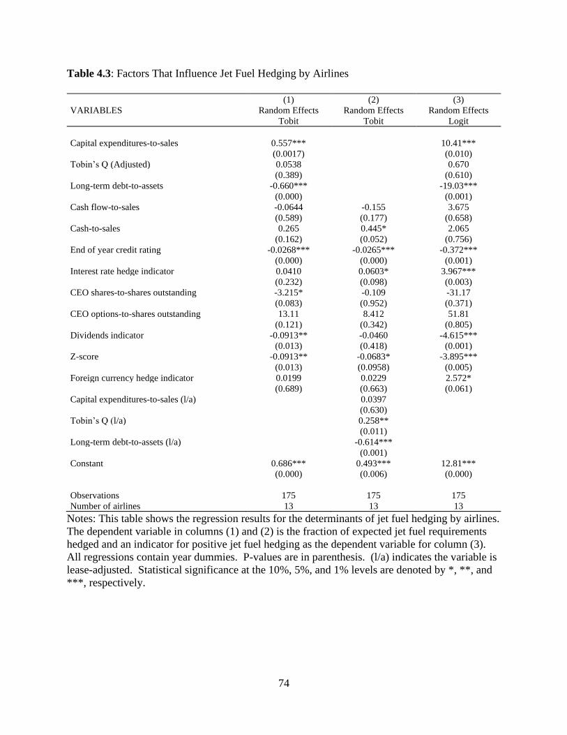
74

Table 4.3: Factors That Influence Jet Fuel Hedging by Airlines

(1) (2) (3)

VARIABLES Random Effects

Tobit

Random Effects

Tobit

Random Effects

Logit

Capital expenditures-to-sales 0.557*** 10.41***

(0.0017) (0.010)

Tobin’s Q (Adjusted) 0.0538 0.670

(0.389) (0.610)

Long-term debt-to-assets -0.660*** -19.03***

(0.000) (0.001)

Cash flow-to-sales -0.0644 -0.155 3.675

(0.589) (0.177) (0.658)

Cash-to-sales 0.265 0.445* 2.065

(0.162) (0.052) (0.756)

End of year credit rating -0.0268*** -0.0265*** -0.372***

(0.000) (0.000) (0.001)

Interest rate hedge indicator 0.0410 0.0603* 3.967***

(0.232) (0.098) (0.003)

CEO shares-to-shares outstanding -3.215* -0.109 -31.17

(0.083) (0.952) (0.371)

CEO options-to-shares outstanding 13.11 8.412 51.81

(0.121) (0.342) (0.805)

Dividends indicator -0.0913** -0.0460 -4.615***

(0.013) (0.418) (0.001)

Z-score -0.0913** -0.0683* -3.895***

(0.013) (0.0958) (0.005)

Foreign currency hedge indicator 0.0199 0.0229 2.572*

(0.689) (0.663) (0.061)

Capital expenditures-to-sales (l/a) 0.0397

(0.630)

Tobin’s Q (l/a) 0.258**

(0.011)

Long-term debt-to-assets (l/a) -0.614***

(0.001)

Constant 0.686*** 0.493*** 12.81***

(0.000) (0.006) (0.000)

Observations 175 175 175

Number of airlines 13 13 13

Notes: This table shows the regression results for the determinants of jet fuel hedging by airlines.

The dependent variable in columns (1) and (2) is the fraction of expected jet fuel requirements

hedged and an indicator for positive jet fuel hedging as the dependent variable for column (3).

All regressions contain year dummies. P-values are in parenthesis. (l/a) indicates the variable is

lease-adjusted. Statistical significance at the 10%, 5%, and 1% levels are denoted by *, **, and

***, respectively.

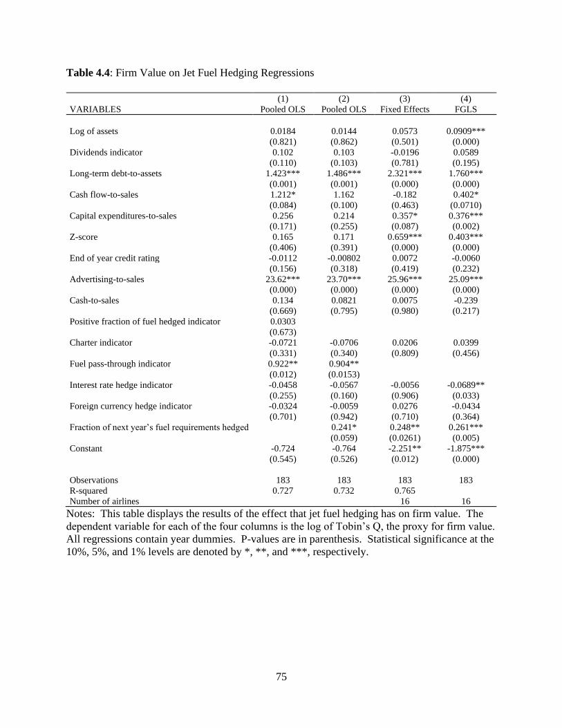
75

Table 4.4: Firm Value on Jet Fuel Hedging Regressions

(1) (2) (3) (4)

VARIABLES Pooled OLS Pooled OLS Fixed Effects FGLS

Log of assets 0.0184 0.0144 0.0573 0.0909***

(0.821) (0.862) (0.501) (0.000)

Dividends indicator 0.102 0.103 -0.0196 0.0589

(0.110) (0.103) (0.781) (0.195)

Long-term debt-to-assets 1.423*** 1.486*** 2.321*** 1.760***

(0.001) (0.001) (0.000) (0.000)

Cash flow-to-sales 1.212* 1.162 -0.182 0.402*

(0.084) (0.100) (0.463) (0.0710)

Capital expenditures-to-sales 0.256 0.214 0.357* 0.376***

(0.171) (0.255) (0.087) (0.002)

Z-score 0.165 0.171 0.659*** 0.403***

(0.406) (0.391) (0.000) (0.000)

End of year credit rating -0.0112 -0.00802 0.0072 -0.0060

(0.156) (0.318) (0.419) (0.232)

Advertising-to-sales 23.62*** 23.70*** 25.96*** 25.09***

(0.000) (0.000) (0.000) (0.000)

Cash-to-sales 0.134 0.0821 0.0075 -0.239

(0.669) (0.795) (0.980) (0.217)

Positive fraction of fuel hedged indicator 0.0303

(0.673)

Charter indicator -0.0721 -0.0706 0.0206 0.0399

(0.331) (0.340) (0.809) (0.456)

Fuel pass-through indicator 0.922** 0.904**

(0.012) (0.0153)

Interest rate hedge indicator -0.0458 -0.0567 -0.0056 -0.0689**

(0.255) (0.160) (0.906) (0.033)

Foreign currency hedge indicator -0.0324 -0.0059 0.0276 -0.0434

(0.701) (0.942) (0.710) (0.364)

Fraction of next year’s fuel requirements hedged 0.241* 0.248** 0.261***

(0.059) (0.0261) (0.005)

Constant -0.724 -0.764 -2.251** -1.875***

(0.545) (0.526) (0.012) (0.000)

Observations 183 183 183 183

R-squared 0.727 0.732 0.765

Number of airlines 16 16

Notes: This table displays the results of the effect that jet fuel hedging has on firm value. The

dependent variable for each of the four columns is the log of Tobin’s Q, the proxy for firm value.

All regressions contain year dummies. P-values are in parenthesis. Statistical significance at the

10%, 5%, and 1% levels are denoted by *, **, and ***, respectively.

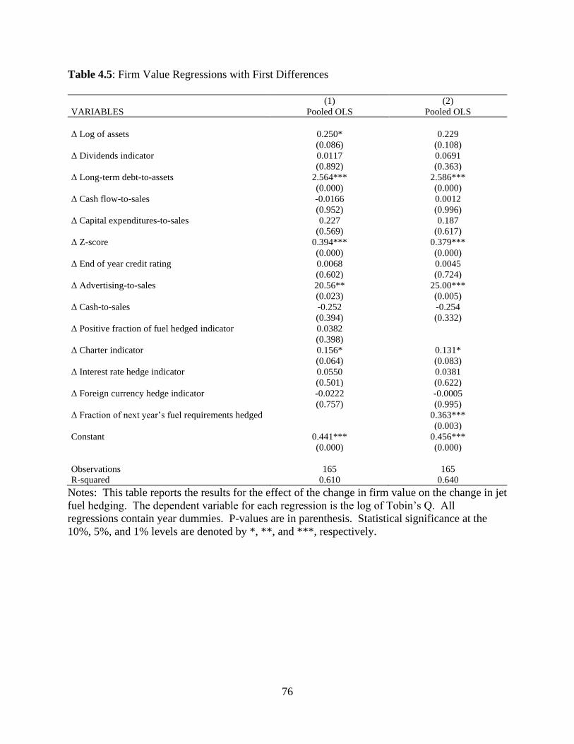
76

Table 4.5: Firm Value Regressions with First Differences

(1) (2)

VARIABLES Pooled OLS Pooled OLS

Δ Log of assets 0.250* 0.229

(0.086) (0.108)

Δ Dividends indicator 0.0117 0.0691

(0.892) (0.363)

Δ Long-term debt-to-assets 2.564*** 2.586***

(0.000) (0.000)

Δ Cash flow-to-sales -0.0166 0.0012

(0.952) (0.996)

Δ Capital expenditures-to-sales 0.227 0.187

(0.569) (0.617)

Δ Z-score 0.394*** 0.379***

(0.000) (0.000)

Δ End of year credit rating 0.0068 0.0045

(0.602) (0.724)

Δ Advertising-to-sales 20.56** 25.00***

(0.023) (0.005)

Δ Cash-to-sales -0.252 -0.254

(0.394) (0.332)

Δ Positive fraction of fuel hedged indicator 0.0382

(0.398)

Δ Charter indicator 0.156* 0.131*

(0.064) (0.083)

Δ Interest rate hedge indicator 0.0550 0.0381

(0.501) (0.622)

Δ Foreign currency hedge indicator -0.0222 -0.0005

(0.757) (0.995)

Δ Fraction of next year’s fuel requirements hedged 0.363***

(0.003)

Constant 0.441*** 0.456***

(0.000) (0.000)

Observations 165 165

R-squared 0.610 0.640

Notes: This table reports the results for the effect of the change in firm value on the change in jet

fuel hedging. The dependent variable for each regression is the log of Tobin’s Q. All

regressions contain year dummies. P-values are in parenthesis. Statistical significance at the


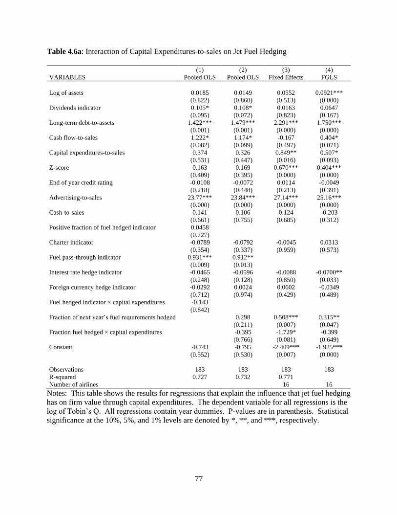
77

Table 4.6a: Interaction of Capital Expenditures-to-sales on Jet Fuel Hedging

(1) (2) (3) (4)


Log of assets 0.0185 0.0149 0.0552 0.0921***

(0.822) (0.860) (0.513) (0.000)

Dividends indicator 0.105* 0.108* 0.0163 0.0647

(0.095) (0.072) (0.823) (0.167)

Long-term debt-to-assets 1.422*** 1.479*** 2.291*** 1.750***

(0.001) (0.001) (0.000) (0.000)

Cash flow-to-sales 1.222* 1.174* -0.167 0.404*

(0.082) (0.099) (0.497) (0.071)

Capital expenditures-to-sales 0.374 0.326 0.849** 0.507*

(0.531) (0.447) (0.016) (0.093)

Z-score 0.163 0.169 0.670*** 0.404***

(0.409) (0.395) (0.000) (0.000)

End of year credit rating -0.0108 -0.0072 0.0114 -0.0049

(0.218) (0.448) (0.213) (0.391)


(0.000) (0.000) (0.000) (0.000)

Cash-to-sales 0.141 0.106 0.124 -0.203

(0.661) (0.755) (0.685) (0.312)

Positive fraction of fuel hedged indicator 0.0458

(0.727)

Charter indicator -0.0789 -0.0792 -0.0045 0.0313

(0.354) (0.337) (0.959) (0.573)

Fuel pass-through indicator 0.931*** 0.912**

(0.009) (0.013)

Interest rate hedge indicator -0.0465 -0.0596 -0.0088 -0.0700**

(0.248) (0.128) (0.850) (0.033)

Foreign currency hedge indicator -0.0292 0.0024 0.0602 -0.0349

(0.712) (0.974) (0.429) (0.489)

Fuel hedged indicator × capital expenditures -0.143

(0.842)

Fraction of next year’s fuel requirements hedged 0.298 0.508*** 0.315**

(0.211) (0.007) (0.047)

Fraction fuel hedged × capital expenditures -0.395 -1.729* -0.399

(0.766) (0.081) (0.649)

Constant -0.743 -0.795 -2.409*** -1.925***

(0.552) (0.530) (0.007) (0.000)


R-squared 0.727 0.732 0.771


Notes: This table shows the results for regressions that explain the influence that jet fuel hedging

has on firm value through capital expenditures. The dependent variable for all regressions is the

log of Tobin’s Q. All regressions contain year dummies. P-values are in parenthesis. Statistical

significance at the 10%, 5%, and 1% levels are denoted by *, **, and ***, respectively.

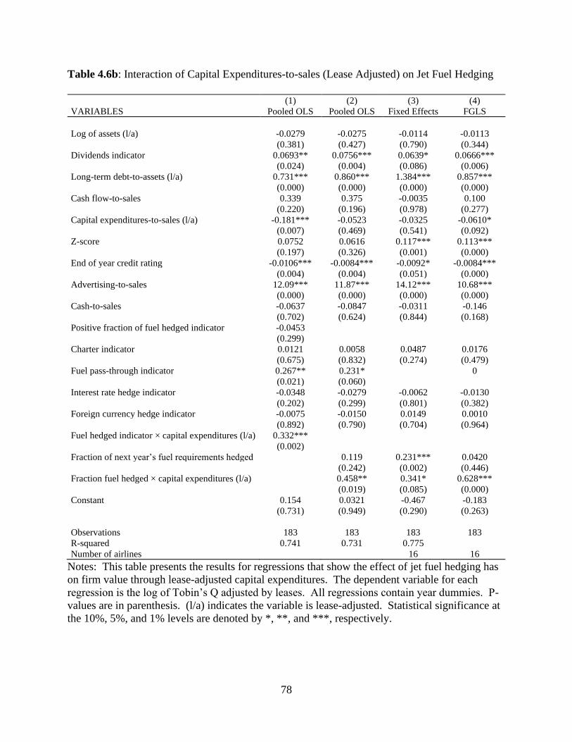
78

Table 4.6b: Interaction of Capital Expenditures-to-sales (Lease Adjusted) on Jet Fuel Hedging

(1) (2) (3) (4)


Log of assets (l/a) -0.0279 -0.0275 -0.0114 -0.0113

(0.381) (0.427) (0.790) (0.344)

Dividends indicator 0.0693** 0.0756*** 0.0639* 0.0666***

(0.024) (0.004) (0.086) (0.006)

Long-term debt-to-assets (l/a) 0.731*** 0.860*** 1.384*** 0.857***

(0.000) (0.000) (0.000) (0.000)

Cash flow-to-sales 0.339 0.375 -0.0035 0.100

(0.220) (0.196) (0.978) (0.277)

Capital expenditures-to-sales (l/a) -0.181*** -0.0523 -0.0325 -0.0610*

(0.007) (0.469) (0.541) (0.092)

Z-score 0.0752 0.0616 0.117*** 0.113***

(0.197) (0.326) (0.001) (0.000)

End of year credit rating -0.0106*** -0.0084*** -0.0092* -0.0084***

(0.004) (0.004) (0.051) (0.000)


(0.000) (0.000) (0.000) (0.000)

Cash-to-sales -0.0637 -0.0847 -0.0311 -0.146

(0.702) (0.624) (0.844) (0.168)

Positive fraction of fuel hedged indicator -0.0453

(0.299)

Charter indicator 0.0121 0.0058 0.0487 0.0176

(0.675) (0.832) (0.274) (0.479)

Fuel pass-through indicator 0.267** 0.231* 0

(0.021) (0.060)

Interest rate hedge indicator -0.0348 -0.0279 -0.0062 -0.0130

(0.202) (0.299) (0.801) (0.382)

Foreign currency hedge indicator -0.0075 -0.0150 0.0149 0.0010

(0.892) (0.790) (0.704) (0.964)

Fuel hedged indicator × capital expenditures (l/a) 0.332***

(0.002)

Fraction of next year’s fuel requirements hedged 0.119 0.231*** 0.0420

(0.242) (0.002) (0.446)

Fraction fuel hedged × capital expenditures (l/a) 0.458** 0.341* 0.628***

(0.019) (0.085) (0.000)

Constant 0.154 0.0321 -0.467 -0.183

(0.731) (0.949) (0.290) (0.263)


R-squared 0.741 0.731 0.775


Notes: This table presents the results for regressions that show the effect of jet fuel hedging has

on firm value through lease-adjusted capital expenditures. The dependent variable for each

regression is the log of Tobin’s Q adjusted by leases. All regressions contain year dummies. P-

values are in parenthesis. (l/a) indicates the variable is lease-adjusted. Statistical significance at

the 10%, 5%, and 1% levels are denoted by *, **, and ***, respectively.

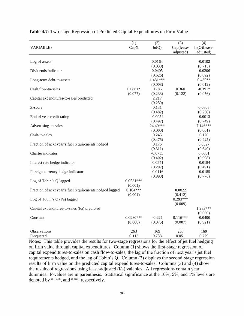
79

Table 4.7: Two-stage Regression of Predicted Capital Expenditures on Firm Value

(1) (2) (3) (4)

VARIABLES CapX ln(Q) Cap(lease-

adjusted)

ln(Q)(lease-

adjusted)

Log of assets 0.0164 -0.0102

(0.830) (0.713)

Dividends indicator 0.0405 -0.0206

(0.526) (0.692)

Long-term debt-to-assets 1.431*** 0.430**

(0.003) (0.012)

Cash flow-to-sales 0.0861* 0.786 0.360 -0.391*

(0.077) (0.233) (0.122) (0.056)

Capital expenditures-to-sales predicted 2.217

(0.259)

Z-score 0.131 0.0808

(0.482) (0.260)

End of year credit rating -0.0054 -0.0013

(0.497) (0.749)

Advertising-to-sales 24.49*** 7.146***

(0.000) (0.001)

Cash-to-sales 0.245 0.120

(0.475) (0.425)

Fraction of next year’s fuel requirements hedged 0.176 0.0327

(0.311) (0.640)

Charter indicator -0.0753 0.0001

(0.402) (0.998)

Interest rate hedge indicator -0.0541 -0.0184

(0.207) (0.491)

Foreign currency hedge indicator -0.0116 -0.0185

(0.890) (0.776)

Log of Tobin’s Q lagged 0.0531***

(0.001)

Fraction of next year’s fuel requirements hedged lagged 0.104*** 0.0822

(0.001) (0.412)

Log of Tobin’s Q (l/a) lagged 0.293***

(0.009)

Capital expenditures-to-sales (l/a) predicted 1.283***

(0.000)

Constant 0.0980*** -0.924 0.116*** -0.0400

(0.000) (0.375) (0.007) (0.921)


R-squared 0.113 0.733 0.051 0.729

Notes: This table provides the results for two-stage regressions for the effect of jet fuel hedging

on firm value through capital expenditures. Column (1) shows the first-stage regression of

capital expenditures-to-sales on cash flow-to-sales, the lag of the fraction of next year’s jet fuel

requirements hedged, and the lag of Tobin’s Q. Column (2) displays the second-stage regression

results of firm value on the predicted capital expenditures-to-sales. Columns (3) and (4) show

the results of regressions using lease-adjusted (l/a) vaiables. All regressions contain year

dummies. P-values are in parenthesis. Statistical significance at the 10%, 5%, and 1% levels are

denoted by *, **, and ***, respectively.

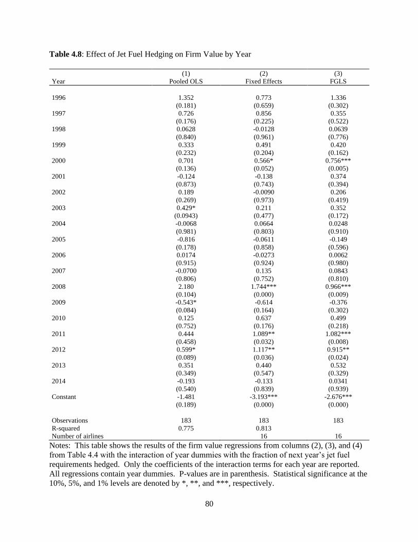
80

Table 4.8: Effect of Jet Fuel Hedging on Firm Value by Year

(1) (2) (3)

Year Pooled OLS Fixed Effects FGLS

1996 1.352 0.773 1.336

(0.181) (0.659) (0.302)

1997 0.726 0.856 0.355

(0.176) (0.225) (0.522)

1998 0.0628 -0.0128 0.0639

(0.840) (0.961) (0.776)

1999 0.333 0.491 0.420

(0.232) (0.204) (0.162)

2000 0.701 0.566* 0.756***

(0.136) (0.052) (0.005)

2001 -0.124 -0.138 0.374

(0.873) (0.743) (0.394)

2002 0.189 -0.0090 0.206

(0.269) (0.973) (0.419)

2003 0.429* 0.211 0.352

(0.0943) (0.477) (0.172)

2004 -0.0068 0.0664 0.0248

(0.981) (0.803) (0.910)

2005 -0.816 -0.0611 -0.149

(0.178) (0.858) (0.596)

2006 0.0174 -0.0273 0.0062

(0.915) (0.924) (0.980)

2007 -0.0700 0.135 0.0843

(0.806) (0.752) (0.810)

2008 2.180 1.744*** 0.966***

(0.104) (0.000) (0.009)

2009 -0.543* -0.614 -0.376

(0.084) (0.164) (0.302)

2010 0.125 0.637 0.499

(0.752) (0.176) (0.218)

2011 0.444 1.089** 1.082***

(0.458) (0.032) (0.008)

2012 0.599* 1.117** 0.915**

(0.089) (0.036) (0.024)

2013 0.351 0.440 0.532

(0.349) (0.547) (0.329)

2014 -0.193 -0.133 0.0341

(0.540) (0.839) (0.939)

Constant -1.481 -3.193*** -2.676***

(0.189) (0.000) (0.000)


R-squared 0.775 0.813


Notes: This table shows the results of the firm value regressions from columns (2), (3), and (4)

from Table 4.4 with the interaction of year dummies with the fraction of next year’s jet fuel

requirements hedged. Only the coefficients of the interaction terms for each year are reported.

All regressions contain year dummies. P-values are in parenthesis. Statistical significance at the


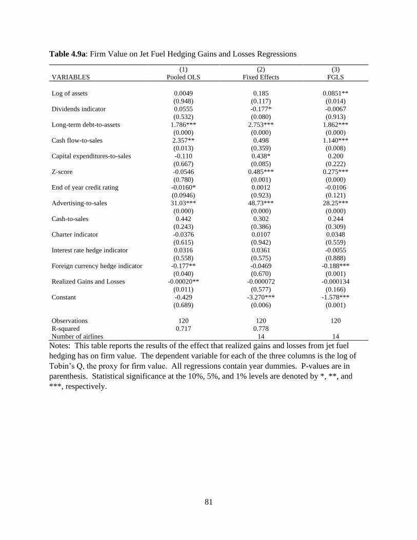
81

Table 4.9a: Firm Value on Jet Fuel Hedging Gains and Losses Regressions

(1) (2) (3)

VARIABLES Pooled OLS Fixed Effects FGLS

Log of assets 0.0049 0.185 0.0851**

(0.948) (0.117) (0.014)

Dividends indicator 0.0555 -0.177* -0.0067

(0.532) (0.080) (0.913)

Long-term debt-to-assets 1.786*** 2.753*** 1.862***

(0.000) (0.000) (0.000)

Cash flow-to-sales 2.357** 0.498 1.140***

(0.013) (0.359) (0.008)

Capital expenditures-to-sales -0.110 0.438* 0.200

(0.667) (0.085) (0.222)

Z-score -0.0546 0.485*** 0.275***

(0.780) (0.001) (0.000)

End of year credit rating -0.0160* 0.0012 -0.0106

(0.0946) (0.923) (0.121)

Advertising-to-sales 31.03*** 48.73*** 28.25***

(0.000) (0.000) (0.000)

Cash-to-sales 0.442 0.302 0.244

(0.243) (0.386) (0.309)

Charter indicator -0.0376 0.0107 0.0348

(0.615) (0.942) (0.559)

Interest rate hedge indicator 0.0316 0.0361 -0.0055

(0.558) (0.575) (0.888)

Foreign currency hedge indicator -0.177** -0.0469 -0.188***

(0.040) (0.670) (0.001)

Realized Gains and Losses -0.00020** -0.000072 -0.000134

(0.011) (0.577) (0.166)

Constant -0.429 -3.270*** -1.578***

(0.689) (0.006) (0.001)


R-squared 0.717 0.778


Notes: This table reports the results of the effect that realized gains and losses from jet fuel

hedging has on firm value. The dependent variable for each of the three columns is the log of

Tobin’s Q, the proxy for firm value. All regressions contain year dummies. P-values are in

parenthesis. Statistical significance at the 10%, 5%, and 1% levels are denoted by *, **, and

***, respectively.

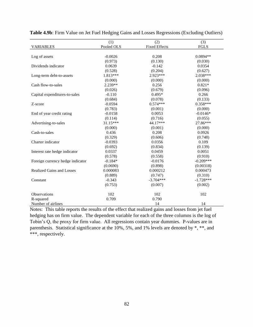
82

Table 4.9b: Firm Value on Jet Fuel Hedging Gains and Losses Regressions (Excluding Outliers)

(1) (2) (3)


Log of assets -0.0026 0.208 0.0894**

(0.973) (0.130) (0.030)

Dividends indicator 0.0639 -0.142 0.0354

(0.528) (0.204) (0.627)


(0.000) (0.000) (0.000)

Cash flow-to-sales 2.239** 0.256 0.821*

(0.026) (0.679) (0.096)

Capital expenditures-to-sales -0.110 0.495* 0.266

(0.684) (0.078) (0.133)

Z-score -0.0594 0.574*** 0.358***

(0.783) (0.001) (0.000)

End of year credit rating -0.0158 0.0053 -0.0146*

(0.114) (0.716) (0.055)


(0.000) (0.001) (0.000)

Cash-to-sales 0.436 0.208 0.0926

(0.329) (0.606) (0.748)


(0.692) (0.834) (0.139)

Interest rate hedge indicator 0.0337 0.0459 0.0051

(0.578) (0.558) (0.910)

Foreign currency hedge indicator -0.184* -0.0176 -0.209***

(0.0690) (0.898) (0.00318)

Realized Gains and Losses 0.000083 0.000212 0.000473

(0.889) (0.747) (0.310)

Constant -0.343 -3.704*** -1.728***

(0.753) (0.007) (0.002)


R-squared 0.709 0.790


Notes: This table reports the results of the effect that realized gains and losses from jet fuel

hedging has on firm value. The dependent variable for each of the three columns is the log of

Tobin’s Q, the proxy for firm value. All regressions contain year dummies. P-values are in


***, respectively.

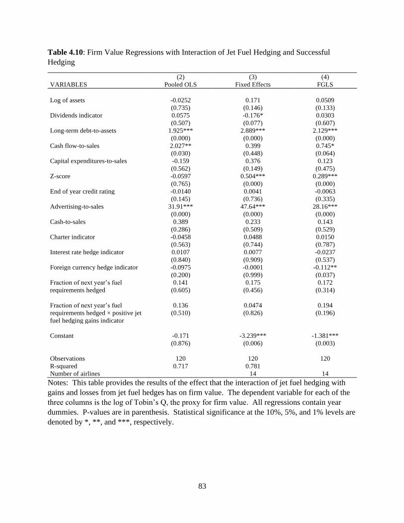
83

Table 4.10: Firm Value Regressions with Interaction of Jet Fuel Hedging and Successful

Hedging

(2) (3) (4)


Log of assets -0.0252 0.171 0.0509

(0.735) (0.146) (0.133)

Dividends indicator 0.0575 -0.176* 0.0303

(0.507) (0.077) (0.607)


(0.000) (0.000) (0.000)

Cash flow-to-sales 2.027** 0.399 0.745*

(0.030) (0.448) (0.064)

Capital expenditures-to-sales -0.159 0.376 0.123

(0.562) (0.149) (0.475)

Z-score -0.0597 0.504*** 0.289***

(0.765) (0.000) (0.000)

End of year credit rating -0.0140 0.0041 -0.0063

(0.145) (0.736) (0.335)


(0.000) (0.000) (0.000)

Cash-to-sales 0.389 0.233 0.143

(0.286) (0.509) (0.529)


(0.563) (0.744) (0.787)

Interest rate hedge indicator 0.0107 0.0077 -0.0237

(0.840) (0.909) (0.537)

Foreign currency hedge indicator -0.0975 -0.0001 -0.112**

(0.200) (0.999) (0.037)

Fraction of next year’s fuel

requirements hedged

0.141

(0.605)

0.175

(0.456)

0.172

(0.314)

Fraction of next year’s fuel

requirements hedged × positive jet

fuel hedging gains indicator

0.136

(0.510)

0.0474

(0.826)

0.194

(0.196)

Constant -0.171 -3.239*** -1.381***

(0.876) (0.006) (0.003)


R-squared 0.717 0.781


Notes: This table provides the results of the effect that the interaction of jet fuel hedging with

gains and losses from jet fuel hedges has on firm value. The dependent variable for each of the

three columns is the log of Tobin’s Q, the proxy for firm value. All regressions contain year

dummies. P-values are in parenthesis. Statistical significance at the 10%, 5%, and 1% levels are

denoted by *, **, and ***, respectively.

84

CHAPTER FIVE:

USING SUCCESSFUL JET FUEL HEDGES TO INCREASE MARKET SHARE

5.1 Investment Opportunities in the Airline Industry

A common problem in the airline industry is underinvestment. This is especially true when the

price of jet fuel is high, resulting in low cash flows. Although profitable investment projects

may exist, airlines may have insufficient financial capital to undertake them. Froot, Scharfstein,

and Stein (1993) suggest that firms hedge to increase cash flows during these low cash flow

states in order to fund investments they would not be able to undertake otherwise. As explained

in chapter one, airlines commonly hedge the price of jet fuel jet fuel prices are highly volatile

and jet fuel expenses make up a large percentage of an airline’s operating costs.

Carter, Rogers, and Simkins (2006) investigate jet fuel hedging by airlines to determine if

it increases the value of the firm (which they call the “hedging premium”). They find that a large

portion of the hedging premium comes from capital expenditures. However, they do not discuss

any of the specific investments that airlines undertake to increase value as a result of jet fuel

hedging. In chapter 4, using a more recent and larger sample of years, jet fuel hedging only has a

positive effect on firm value through capital expenditures when lease adjustments are

85

considered.25 Leasing aircraft may play an important role in the investment projects that airlines

fund through hedging.

5.1.1 Investment Project Classifications

When leasing or purchasing aircraft, airlines must decide how they will be allocated. Airlines

typically employ capital budgeting techniques to determine the most profitable uses for their

aircraft. Vasigh, Fleming, and Humphreys (2014) describe the two most common classifications

of investment projects that airlines can undertake: (1) replacement versus expansion decisions

and (2) independent projects versus mutually exclusive projects. In the first classification, newly

acquired aircraft can be used to replace older aircraft or can be utilized to expand into new

markets. If an airline believes that jet fuel prices will increase in the future, replacing older

planes with newer, more fuel-efficient models may be the more profitable option. Additional

profits can be obtained by entering into new markets or increasing capacity in markets they

already serve.

In the second classification, investment projects can be mutually exclusive or

independent. Although many profitable projects may exist, the airline may not be able to fund

all the projects at the same time. For example, if an airline has a choice between two profitable

projects but only has enough financial capital available at the time to fund one of them, the two

projects are categorized as “mutually exclusive.” “Independent projects,” however, can be

funded regardless of the funding status of other available projects. For example, if an airline has

enough financial capital available to fund two projects simultaneously, these projects would be

25 Operating leases (which airlines commonly employ) do not appear on airlines’ balance sheets. Adding the value

of operating leases to capital expenditures is necessary to provide an accurate measure of an airline’s overall

investment.

86

considered independent. Although financially constrained airlines can alleviate the

underinvestment problem with hedging, they may find that any additional projects it wishes to

pursue using the additional cash flows from hedging are likely to be mutually exclusive. These

investment projects must be chosen carefully so that the most profitable one is selected.

Using capital budgeting techniques to make the most profitable investment decisions

rests on the assumption that the managers charged with making these determinations are acting

in a profit-maximizing fashion for the airline. However, when corporate controls are weak,

managers may choose instead to make investment decisions that increase their own personal

utility, oftentimes at the expense of the firm. The following section explains how hedging can

further exacerbate agency issues.

5.1.2 Principal-agent Problems, Buying Market Share, and Hedging

A section of the hedging literature discusses principal-agent problems that can arise when firms

hire managers to make hedging decisions. Smith and Stulz (1985) argue that managers may

choose a hedging portfolio that maximizes their own utility at the expense of increasing

shareholder wealth. This generally occurs when managerial compensation incentives do not

align with the firm objective of profit maximization. For example, if the manager’s

compensation package includes more stock options, then the manager may choose to hedge less

so that the firm’s value (as reflected by the firm’s stock price) has higher variability. This

improves the probability that the manager’s stock options can be exercised profitably.

Tufano (1998) identifies a second possible agency issue in which managers use the

increased cash flows from hedging on investment projects that increase personal utility but are

value destroying to the firm. Financing investment using funds internal to the firm is generally

87

preferable to seeking funding through capital markets because potential lenders are more likely

to decline financing to projects they believe will be unprofitable. If the firm has insufficient

internal funds to finance its investments, managers may turn to hedging to increase internal funds

and avoid the increased scrutiny of outside lenders. Without the input of capital markets,

managers are more likely to invest in projects that benefit themselves but make shareholders

worse off.

Hedging may also exacerbate the agency problem between a manager’s desire to

maximize personal utility and the firm objective of maximizing shareholder wealth. The first

two cases described previously assume managers are acting in their own interest at the expense

of shareholders. However, agency issues may also arise when managers have a

misunderstanding of the objectives a firm should pursue or what constitutes profit-maximizing

behavior. Hedging can make pursuing these objectives more attractive to managers, especially

when the firm has a run of success with its hedges.

A common misconception that can arise among firms, explained in detail by Thomas and

Kamp (2006), is the belief that increasing market share is a way to achieve greater profitability

or that acquiring higher market share is the primary goal of the firm, even if profits suffer. One

possible way to achieve increases in market share is for managers to price their goods and

services below the profit-maximizing price, a pricing strategy called “buying market share.” If

the short-term losses from lowering price cannot be recouped in a later time period, then this

pricing strategy will reduce the value of the firm. This strategy raises the question of possible

predatory pricing since both require the lowering of price its profit-maximizing level.26

26 Predatory pricing is a pricing strategy where firms lower their price below cost with the purpose of driving rivals

out of the market, then attempt to recoup losses by raising price above cost after they exit. This is only successful if

barriers to entry are sufficiently high so that other firms cannot enter (or reenter) once predatory firm raises its price.

88

However, predatory pricing requires a high likelihood that short-run losses can be recouped but

buying market share does not.

Managers who engage in buying market share may also have the decision to do so

reinforced by an increase in their personal utility, especially if managers’ compensation is tied to

the relative market shares of the firms. As the market share of the firm increases, so will the

compensation that is received by the manager, even as the profits of the firm fall. Creating

compensation packages for managers that encourage buying market share behavior can lead to

reduced shareholder wealth.

Hedging may influence a manager’s decision to buy market share. When hedging is

successful, the increased cash flow can be “invested” by lowering the price of the goods or

services sold to consumers, in effect buying market share the firm would not be able to attain

without hedging. For example, if an airline has successful jet fuel hedges, managers may

mistakenly believe that the cost of using jet fuel has decreased. This is not the case, as explained

in chapter one, because the cost of using jet fuel is not the price paid for it, but the price that the

airline could receive by selling it on the open market. Although costs have not changed as a

result of hedging, managers may still attempt to pass on the “savings” to consumers in the form

of lower fares which can increase market share. This pricing strategy is likely not profit

maximizing as the airline is pricing below its profit-maximizing level, even if it mistakenly does

not believe that it is.

5.2 Changes in Market Share and Jet Fuel Hedging Gains and Losses

It follows from the proceeding discussion that successful jet fuel hedging by airlines may be used

to buy market share. However, there has been no empirical study on this question to date. It is

89

useful to first determine the association between positive gains from jet fuel hedges and changes

in market share. If jet fuel hedging success leads to buying market share, then a positive

relationship between realized gains and losses from jet fuel hedging and changes in market share

is expected.

It is important to note, however, that finding a positive relationship between realized

gains and losses and jet fuel hedging is not sufficient to indicate that buying market share is

taking place. An increase in market share may also appear when an airline enters a new market,

that is, the market share of the airline increases from zero to a positive number. Care must be

taken to account for this possibility when analyzing the data.

5.2.1 Airline Selection, Realized Gains and Losses, and Time Frame

The sample of airlines used in to calculate the market shares used in this chapter are taken from

major carriers that hedge a significant portion of their jet fuel requirements. Typically, smaller

low-cost carriers use other forms of jet fuel risk management such as fuel pass-through

agreements or charter operations that pass on the cost of fuel to other parties. Smaller carriers

are much less likely to engage in any kind of buying market share pricing scheme since they

would be unable to handle the initial loss of profits that would result. Smaller carriers also tend

to leave the larger airlines to compete amongst themselves.

Figure 5.1 shows the realized gains and losses from jet fuel hedging for the sample

airlines. Because hedging data were unreliable prior to the passage of FAS 133 in 2001, the

analysis begins in 2000 and ends in 2013. The time-series for hedging data are cut short for

some airlines due to mergers between major carriers. Northwest Airlines, for example, merged

90

with Delta Air Lines in 2008, followed by a merger of Continental Airlines and United Airlines

in 2010, and US Airways and American Airlines in 2013.

Southwest Airlines gained notoriety for undertaking a series of highly successful jet fuel

hedges from 2004 to 2008. This allowed Southwest to gain significant cash flows from its

hedges that could be used to expand operations to new markets or pass on savings to consumers

in the form of lower fares. The analyses of the chapter focus heavily on Southwest Airlines with

other airlines considered as robustness checks.

Figure 5.1 shows that, prior to 2009, airlines generally recorded positive gains from their

jet fuel hedging activities. However, when the financial crisis reached its peak in 2009, oil prices

decreased significantly along with jet fuel prices. All hedging airlines suffered losses of varying

degrees. While United Airlines and Delta Air Lines returned to positive jet fuel hedging gains

quickly, Southwest continued to sustain jet fuel hedging losses until 2014. The time frame of the

analyses is broken into two time periods: (1) 2000-2008, and (2) 2009-2013. This corresponds to

the years when Southwest Airlines enjoyed jet fuel hedging gains pre-financial crisis but suffered

hedging losses post-financial crisis.

5.2.2 Market Definitions

Episodes of buying market share do not necessarily have to be nationwide, and so it is important

to break down an airline’s operations into smaller markets. The definition of a market used in

this study is taken from the Federal Aviation Administration’s (FAA) definition of a city-pair

market. The FAA describes a city pair as a city of origin and a corresponding destination city for

flights to and from major metropolitan areas (“City Pairs,” 2018). For example, a flight from

91

Tampa, Florida to Phoenix, Arizona and a separate flight from Phoenix, Arizona to Tampa,

Florida would be in a single market.

As a robustness check, a narrower definition of a market is considered in this study. The

narrowest definition of a market would consider flights to and from distinct airports as separate

and unique markets. Furthermore, since some of the larger city-pair markets are served by

multiple airports, this study defines each route combination between two airports as separate

markets, even when the airports operate within the same city market.27

5.2.3 Measuring Changes in Market Share

An airline’s market share for a given market is determined by the fraction of passengers it flies in

the market yearly relative to the total number of passengers flown in the market yearly by all

airlines in the sample. The changes in market share are measured in four separate ways with

each measure of the change in market share being distinguished by the superscripts in equations

(1)-(4). The first two measures consider the change in market share between the endpoints of

each time period, 2000 and 2008 in the first time period, and 2009 and 2013 in the second time

period. The first measure of the change in market share, S1, is the absolute change in market

share between the endpoints for each time period, defined as follows.

𝑆𝑖,11 = 𝑠𝑖,2008 − 𝑠𝑖,2000 (1a)

𝑆𝑖,21 = 𝑠𝑖,2013 − 𝑠𝑖,2008 (1b)

27 For example, Dallas Love Field (DAL) and Dallas/Fort Worth International Airport (DFW) serve the same market

and form a city-pair market with Louisville, Kentucky which is solely served by Louisville International Airport

(SDF). Using the narrowest definition of a market, the route combinations between these airports would form four

separate markets (DAL to SDF, DFW to SDF, SDF to DAL, and SDF to DFW).

92

where 𝑆𝑖,11 and 𝑆𝑖,2

1 are the absolute changes in market share in market i for time periods 1 and 2,

respectively, and si,t is the market share in market i in year t, with t being the years of the

endpoints for each of the time periods 1 and 2. The second measure of the change in market

share, S2, is the proportional change in market share between the endpoints for each time period,

with expressions shown below.

𝑆𝑖,1

2 =𝑠𝑖,2008 − 𝑠𝑖,2000

(𝑠𝑖,2008 + 𝑠𝑖,2000

2)

(2a)

𝑆𝑖,2

2 =𝑠𝑖,2013 − 𝑠𝑖,2008

(𝑠𝑖,2013 + 𝑠𝑖,2009

2 )

(2b)

where 𝑆𝑖,12 and 𝑆𝑖,1

2 are the proportional changes in market share in market i for time periods 1

and 2, respectively, and si,t defined above. In equations (2a) and (2b), the denominator of the

right-hand side is the average market share between the endpoints of each time period.

These two measures provide a simple look at how market share changes for each airline

from the beginning to the end of each time period. However, the disadvantage of calculating the

change in market share in these two ways is that is does not give a clear picture on how market

share changes between the end points of each time period. The airline may enter or exit a market

between end points or other airlines may enter or leave. Mergers between airlines may also

occur.

The third and fourth measures of the change in market share, defined by S3 and S4,

respectively, observe the change in market share from year to year. These measures of the

change in market share are calculated using the following equations:

𝑆𝑖,𝑡3 = 𝑠𝑖,𝑡 − 𝑠𝑖,𝑡−1 (3)

93

𝑆𝑖,𝑡

4 =𝑠𝑖,𝑡 − 𝑠𝑖,𝑡−1

(𝑠𝑖,𝑡 + 𝑠𝑖,𝑡−1

2 )

(4)

where 𝑆𝑖,𝑡3 is the absolute change in market share in market i at year t, and 𝑆𝑖,𝑡

4 is the proportional

change in market share in market i at time t. si,t and si,t-1 are the market shares in market i at

times t and t-1, respectively. In these measures of the change in market share, the years 2000

and 2009 are excluded because each is the first year of their respective time periods. In equation

(4), the denominator of the right-hand side is the average market share between year t and year t-

1.

5.2.4 Model for Changes in Market Share and Hedging Gains and Losses

The base model for the analyses is a simple regression model between the change in market

share and an indicator variable for jet fuel hedging gains and losses. The indicator variable for

hedging gains and losses is formally defined below.

𝐻𝑡 = {1, 𝑗𝑒𝑡 𝑓𝑢𝑒𝑙 ℎ𝑒𝑑𝑔𝑖𝑛𝑔 𝑔𝑎𝑖𝑛𝑠/𝑙𝑜𝑠𝑠𝑒𝑠 > 00, 𝑗𝑒𝑡 𝑓𝑢𝑒𝑙 ℎ𝑒𝑑𝑔𝑖𝑛𝑔 𝑔𝑎𝑖𝑛𝑠/𝑙𝑜𝑠𝑠𝑒𝑠 ≤ 0

(5)

Ht is 1 when an airline experiences gains in its jet fuel hedging activities in year t and 0 when it

has zero gains or losses or suffers losses from its jet fuel hedges in year t. The relationship

between changes in market share and jet fuel hedging is determined by the following model:

𝑆𝑖𝑡 = 𝛽0 + 𝛽1𝐻𝑡 + 𝑢 (6)

where Sit is the change in market share in market i at time t, Ht is the jet fuel hedging gain or loss

indicator at time t, and u is the idiosyncratic error term.

The model is run separately for each individual airline. The model is also run for each

measure of market share described in section 5.2.3. Moreover, restrictions are placed on which

markets are included in the sample. Individual airlines do not fly passengers in every available

94

market, nor do airlines fly passengers every year in a market (i.e., airlines commonly enter and

exit markets over time). Restricting the sample eliminates markets that are very small or not

relevant to an airline’s operations. Specific restrictions on the market samples used in the model

are discussed in the next section.

5.2.5 Restrictions on the Market Sample

The restrictions imposed on the sample of markets depends on the change in market share

measures used in the model. For the change in market share measures in equations (1a), (1b),

(2a) and (2b), the market sample is restricted by the number of time periods in which an airline

flies a positive number of passengers at the beginning or end year of the time period. Each

market only has two observations: the first observation is the change in market share in the 2000

and 2008 time period, and the second observation is the change in market share in the 2009 and

2013 time period. Therefore, each market will fall under one of three possible cases.

1. Case 1: An airline flies a positive number of passengers in none of the time periods.

This means that 𝑠𝑖,2000 = 0 and 𝑠𝑖,2008 = 0, and 𝑠𝑖,2009 = 0 and 𝑠𝑖,2013 = 0.

2. Case 2: An airline flies a positive number of passengers at some point in one of the time

periods. That is, 𝑠𝑖,2000 > 0 or 𝑠𝑖,2008 > 0, and no passengers are flown in 2009 and

2013, or there are no passengers flown in 2000 and 2008, and 𝑠𝑖,2009 > 0 or 𝑠𝑖,2013 > 0.

3. Case 3: An airline flies a positive number of passengers at some point in two time

periods. This requires that 𝑠𝑖,2000 > 0 or 𝑠𝑖,2008 > 0, and 𝑠𝑖,2009 > 0 or 𝑠𝑖,2013 > 0.

The possible restrictions on the market sample using these cases are defined by RK, where K is

the minimum number of time periods where the airline flies a positive number of passengers.

Letting ki be number of time periods where the airline flies a positive number of passengers in

95

market i, restriction RK is defined as follows: keep any market i that satisfies the following

condition.

𝑘𝑖 ≥ 𝐾 (7)

For example, the R1 restriction requires that all markets fall under case 1 or case 2 described

above. R2 represents the most restrictive sample where only the markets that fall under case 3

are kept in the sample. R0 defines the sample of markets with no restrictions.

For the year-to-year changes in market share described in equations (3) and (4), market

restrictions are based on the number of years in which an airline has zero market share in market

i. These restrictions are defined as ZM, where M is the minimum number of years in which an

airline’s market share is zero in a market. If mi is the number of years that an airline operates in

market i, then restriction ZM is defined as follows: keep any market i that satisfies the following

condition.

𝑚𝑖 ≥ 𝑀 (8)

For example, Z6 restricts the market sample to markets in which the airline operates for at least

six years (markets where the airline operates for 5 years or fewer are dropped). The broadest

restriction, Z14, describes a market sample in which an airline operates in each market for every

year in the both time periods. Z0 defines an unrestricted market sample.

5.3 Analysis of Market Sample and Estimation Results for Southwest Airlines

The primary airline considered in the model is Southwest Airlines because of its significant jet

fuel hedging gains from 2000 to 2008 followed by is jet fuel hedging losses from 2009 to 2013.

First, a discussion of the change in market share statistics for Southwest Airlines is provided.

Emphasis is given to how the number of markets is affected by each sample restriction. The

96

mean changes in market share across each time period are compared for each measure of market

share. Second, the model runs of equation (6) using each of the market share measures and

relevant sample restrictions are analyzed. All results of the model are estimated using ordinary

least squares (OLS). Third, robustness checks are performed by narrowing the market definition

to individual airports and running the model for other major airlines. Similar to Southwest, some

airlines, such as American Airlines, hedge significant portions of their jet fuel requirements.

Others, such as Alaska Airlines and JetBlue hedge less of their jet fuel requirements but still

record gains and losses from those hedges.

5.3.1 Market Sample and Sample Restrictions

Table 5.1 displays the number of observations, number of markets, and the change in the number

of markets for each sample restriction for Southwest Airlines. The total number of markets in

the unrestricted sample is 9,465. Removing markets in which Southwest does not fly any

passengers in at least one year of the sample time period reduces the sample to 2,750.

Restricting the sample to markets in which Southwest flies passengers over at least half of the

sample time period (restriction Z7) reduces the sample further to 1,348. The most restrictive

sample, only 591 markets are present. Markets where passengers are more consistently flown

from year to year are less likely to influence change in market share through entry or exit. A

positive effect of jet fuel hedging on market share in these markets can more reasonably be

attributed to airlines investing additional capital (e.g., more aircraft) or buying market share.

Table 5.2 shows the average changes in market share over the two time periods for each

measure of market share and relevant restrictions. For the least restrictive samples, the average

market share is generally larger during the jet fuel hedging losses period than the hedging gains

period. As the sample becomes more restrictive, however, the average change in market share

97

quickly becomes larger during the period with hedging gains. The model is expected to return a

positive correlation between the jet fuel hedging gains indicator and the change in market share

for more restrictive samples.

5.3.2 Estimation Results

Table 5.3 shows the estimation results for the first two change in market share measures

described in equations (1a)-(1b) and equations (2a)-(2b). For each of these measures, the model

is estimated three times: once without any sample restriction (R0), all markets where Southwest

Airlines flies passengers in at least one time period (R1), and all markets where Southwest flies

passengers in both time periods (R2).

The estimate for the successful jet fuel hedging indicator on the change in market share is

slightly negative in the unrestricted sample, highly negative in the R1 sample, but even more

strongly highly positive in the most restrictive sample in which Southwest Airlines operates at

some point in each time period. All three estimates are highly significant. The highly negative

result of the R1 sample may be explained by markets where Southwest exits a market after year

2000 but never reenters for the remainder of the time period. This is likely because the number

of markets in the R1 sample must overlap with markets that are also in the Z1 sample (which

includes markets where Southwest only flies passengers in one or fewer years of the sample time

period).28

The positive coefficient on the jet fuel hedging indicator in the R2 sample may be

explained in two ways. First, Southwest may enter markets after 2000 up to 2008 resulting in a

large increase in market share between the two endpoints of the time period followed by

28 The R1 sample contains 2,496 markets and the Z2 sample contains 2,042 markets, so 454 markets must come from

the Z1 sample (any markets in the Z0 sample cannot be contained in the R1 sample).

98

marginal changes in market share thereafter. Second, Southwest may be increasing capacity

within markets it is already operating in. This can be done by investing further capital resources

into a market or making fares more competitive (provided there is competition with other airlines

within the market). However, this measure of market share makes these two possibilities

impossible to discern from one another because it cannot account for how market share changes

between endpoints of the time period.

Year-to-year market share changes better account for entry or exit of an airline or how it

changes between years of operation. Table 5.4 shows the estimates for the jet fuel hedging

indicator on the change in market share described by equation (3). The hedging indicator

coefficient is positive and significant after eliminating markets in which Southwest operates for

five or fewer years in the sample time period. The largest coefficient on the hedging indicator is

on sample Z7 and remains above 2.000 between samples Z6 and Z9. These market samples

correspond to the length of the jet fuel hedging gains time period from 2000 to 2008. Market

shares are increasing the most during this time compared to Southwest’s hedging losses time

frame. Southwest likely entered markets contained in these samples (Z6 and Z9) prior to 2008

(provided there was no exit and reentry at a later year), increasing its market share.

The most restrictive market samples, such as Z12 and Z13, are of particular interest

because market entry is less likely to be the driving force behind these positive jet fuel hedging

indicator coefficients. The hedging indicator coefficient for these samples, while not as highly

statistically significant as the samples discussed previously, are still significant at standard levels.

This suggests that Southwest could indeed be using its successful jet fuel hedges to expand its

capacity in markets in which it already operates.

99

The estimates in Table 5.5 using the year-to-year proportional change in market share

measure from equation (4) show much of the same behavior described in Table 5.4. The

coefficients show a greater degree of significance across each of the samples. The coefficient in

the most restrictive sample, Z14, becomes significant at the 10% level whereas it was highly

insignificant using the standard change in market share of equation (3). In markets without the

possibility of entry in the sample time period, market share is increasing during periods of jet

fuel hedging gains compared to the time period with hedging losses.

5.3.3 Robustness Checks: Airport Markets and Different Airline Model Estimates

The results for Southwest Airlines in the previous section are compared against two separate

robustness checks. First, the market definition is narrowed so that routes from one airport to

another in a single direction is considered a unique market. Even if an airline flies passengers in

a city-pair market, it may not fly routes in both directions to and from each city market, nor may

it necessarily operate out of all the airports that serve a city market (provided there are multiple

airports serving it). In the narrowed market definition, airports where Southwest does not

operate will be removed in the restricted market samples. Changes in the number of passengers

flown by other airlines at other airports where Southwest does not fly passengers should not

affect the market share of Southwest at the airport in which it does operate.

Second, the model is estimated for other airlines that hedge their jet fuel requirements.

None of the other airlines had the level of success that Southwest Airlines experienced hedging

jet fuel, even though some airlines did experience moderately significant gains prior to 2009.

Three airlines are analyzed with the change in market share model from equation (6): American

Airlines, Alaska Airlines, and JetBlue Airways. These airlines are chosen because they operate

100

within the entire sample time frame and are not a part of major mergers during the middle of the

time frame.29

5.3.3.1 Estimates Using Alternative Market Definition

In this section, the model is estimated using the narrower, one-way airport-to-airport definition

of a market. Table 5.6 displays this model estimate for the jet fuel hedging indicator on the

change in market share measure from equation (4) for Southwest Airlines. Using this narrower

definition of a market, the number of markets in the unrestricted sample more than doubles to

22,506 (from 9,465 markets using the broad market definition). The number of markets remains

approximately double for each sample restriction.

The estimation results for the narrow airport definition of a market show similar behavior

to the estimates using the broad market definition. The coefficients are mostly positive and

highly significant, with the largest coefficient in the Z7 restriction sample (slightly higher than

the Z7 coefficient from Table 5.5). The most restrictive sample has a highly significant hedging

indicator coefficient. At the airport level, the increase in market share during the years of

successful jet fuel hedging by Southwest Airlines remains.

5.3.3.2 Model Estimates for Other Airlines

The change in market share model is run for three other airlines: American Airlines, Alaska

Airlines, and JetBlue Airways. Each of the model runs uses the proportional change in market

share measure from equation (4). All estimates use the broad city-pair market definition used in

the primary analyses.

29 American Airlines officially merged with US Airways on December 9, 2013, the final year of the sample time

period. However, the merger would not be reflected in the passenger data until 2015 when the operating certificates

for the two airlines were combined.

101

American airlines posted jet fuel hedging gains from 2000 to 2008 (hedging data for the

airline is unavailable for 2005 and 2006) but also had two years of hedging gains in 2010 and

2011, both of which occurred after the financial crisis. Table 5.7 shows the model estimates for

American Airlines. Similar to Southwest Airlines, American shows positive and significant

coefficients on the jet fuel hedging indicator variable. The largest coefficient, however, appears

on restriction sample Z9 and do not significantly decrease even in the most restricted samples.

American Airlines shows a greater change in market share during periods of hedging gains, even

when market entry is less likely to drive increases in market share in the more restricted samples.

Table 5.8 and Table 5.9 show the model estimation results for Alaska Airlines and

JetBlue Airways, respectively. Both airlines recorded modest gains and losses from their jet fuel

hedges. Few of the coefficients show consistent statistical significance across sample restrictions

like Southwest and American Airlines. Successful jet fuel hedges have little effect on changes in

market share.

5.4 Conclusion

Firms that hedge can use the increased cash flows to undertake investment that they would be

unable to fund otherwise. These additional investments may be profitable to the firm, however,

agency problems may arise if there is a mismatch between shareholder and manager incentives.

Managers may engage in value-destroying projects to increase their personal utility or wealth at

the expense of shareholder wealth. One such agency problem is buying market share, in which

managers set price below cost to increase the firm’s market share, even if they know that this

pricing behavior will reduce profits. Input price hedging may exacerbate this problem if

managers are convinced that hedging has lowered costs from lower input prices, allowing them

102

to pass on the “savings” to consumers through lower output prices, possibly inadvertently

reducing profits.30

In this chapter, an econometric model is constructed to establish the correlation between

changes in market share of an airline and successful jet fuel hedging. Southwest Airlines is the

primary airline tested in the models because of it was significantly more successful in its jet fuel

hedging activities compared to other hedging airlines. Estimates of the model show a positive

relationship between changes in market share and jet fuel hedging gains and losses across

multiple measures of market share, market sample restrictions, and market definitions. This

positive correlation is also demonstrated for American Airlines which experienced modest jet

fuel hedging gains, but no statistical correlation for Alaska Airlines and JetBlue Airways.

The results in this chapter, despite being positive and statistically significant, only

provide preliminary evidence that airlines with successful hedges may be using the increased

cash flow to increase market share. Further analysis is required to determine if airlines are

possibly engaging in buying market share with successful hedges or investing in capital to

expand into new markets. Future models should incorporate controls for ticket fares, mergers

between airlines, and market entry.

30 Recall that the opportunity cost of using an input is its next highest-valued use. Purchasing an input at a lower

price does not change the opportunity cost of the input.

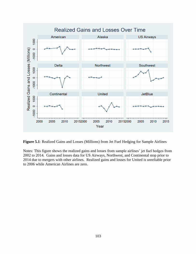
103

Figure 5.1: Realized Gains and Losses (Millions) from Jet Fuel Hedging for Sample Airlines

Notes: This figure shows the realized gains and losses from sample airlines’ jet fuel hedges from

2002 to 2014. Gains and losses data for US Airways, Northwest, and Continental stop prior to

2014 due to mergers with other airlines. Realized gains and losses for United is unreliable prior

to 2006 while American Airlines are zero.

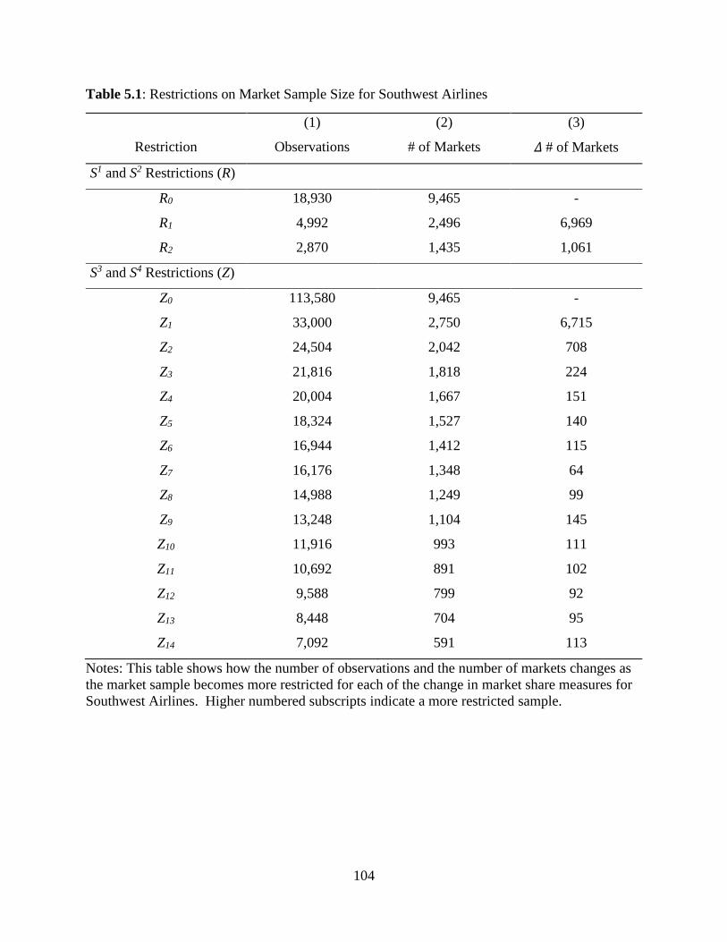
104

Table 5.1: Restrictions on Market Sample Size for Southwest Airlines

(1) (2) (3)

Restriction Observations # of Markets 𝛥 # of Markets

S1 and S2 Restrictions (R)

R0 18,930 9,465 -

R1 4,992 2,496 6,969

R2 2,870 1,435 1,061

S3 and S4 Restrictions (Z)

Z0 113,580 9,465 -

Z1 33,000 2,750 6,715

Z2 24,504 2,042 708

Z3 21,816 1,818 224

Z4 20,004 1,667 151

Z5 18,324 1,527 140

Z6 16,944 1,412 115

Z7 16,176 1,348 64

Z8 14,988 1,249 99

Z9 13,248 1,104 145

Z10 11,916 993 111

Z11 10,692 891 102

Z12 9,588 799 92

Z13 8,448 704 95

Z14 7,092 591 113

Notes: This table shows how the number of observations and the number of markets changes as

the market sample becomes more restricted for each of the change in market share measures for

Southwest Airlines. Higher numbered subscripts indicate a more restricted sample.

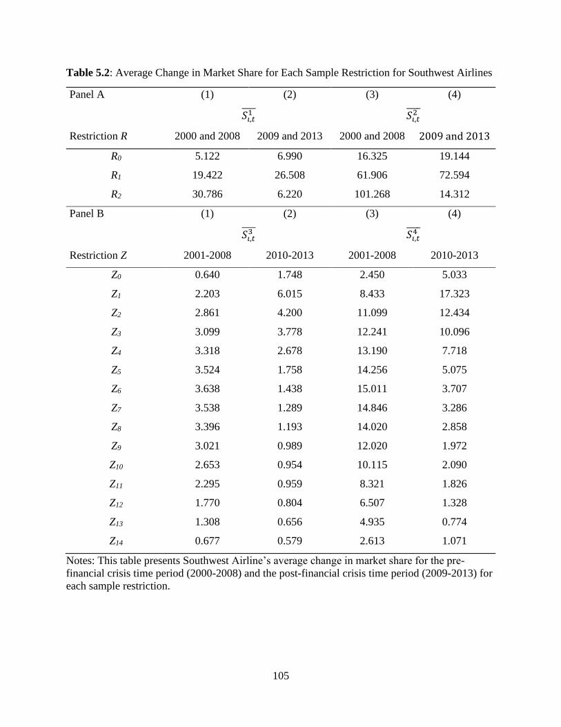
105

Table 5.2: Average Change in Market Share for Each Sample Restriction for Southwest Airlines

Panel A (1) (2) (3) (4)

𝑆𝑖,𝑡1̅̅ ̅̅ 𝑆𝑖,𝑡

2̅̅ ̅̅

Restriction R 2000 and 2008 2009 and 2013 2000 and 2008 2009 and 2013

R0 5.122 6.990 16.325 19.144

R1 19.422 26.508 61.906 72.594

R2 30.786 6.220 101.268 14.312

Panel B (1) (2) (3) (4)

𝑆𝑖,𝑡3̅̅ ̅̅ 𝑆𝑖,𝑡

4̅̅ ̅̅

Restriction Z 2001-2008 2010-2013 2001-2008 2010-2013

Z0 0.640 1.748 2.450 5.033

Z1 2.203 6.015 8.433 17.323

Z2 2.861 4.200 11.099 12.434

Z3 3.099 3.778 12.241 10.096

Z4 3.318 2.678 13.190 7.718

Z5 3.524 1.758 14.256 5.075

Z6 3.638 1.438 15.011 3.707

Z7 3.538 1.289 14.846 3.286

Z8 3.396 1.193 14.020 2.858

Z9 3.021 0.989 12.020 1.972

Z10 2.653 0.954 10.115 2.090

Z11 2.295 0.959 8.321 1.826

Z12 1.770 0.804 6.507 1.328

Z13 1.308 0.656 4.935 0.774

Z14 0.677 0.579 2.613 1.071

Notes: This table presents Southwest Airline’s average change in market share for the pre-

financial crisis time period (2000-2008) and the post-financial crisis time period (2009-2013) for

each sample restriction.

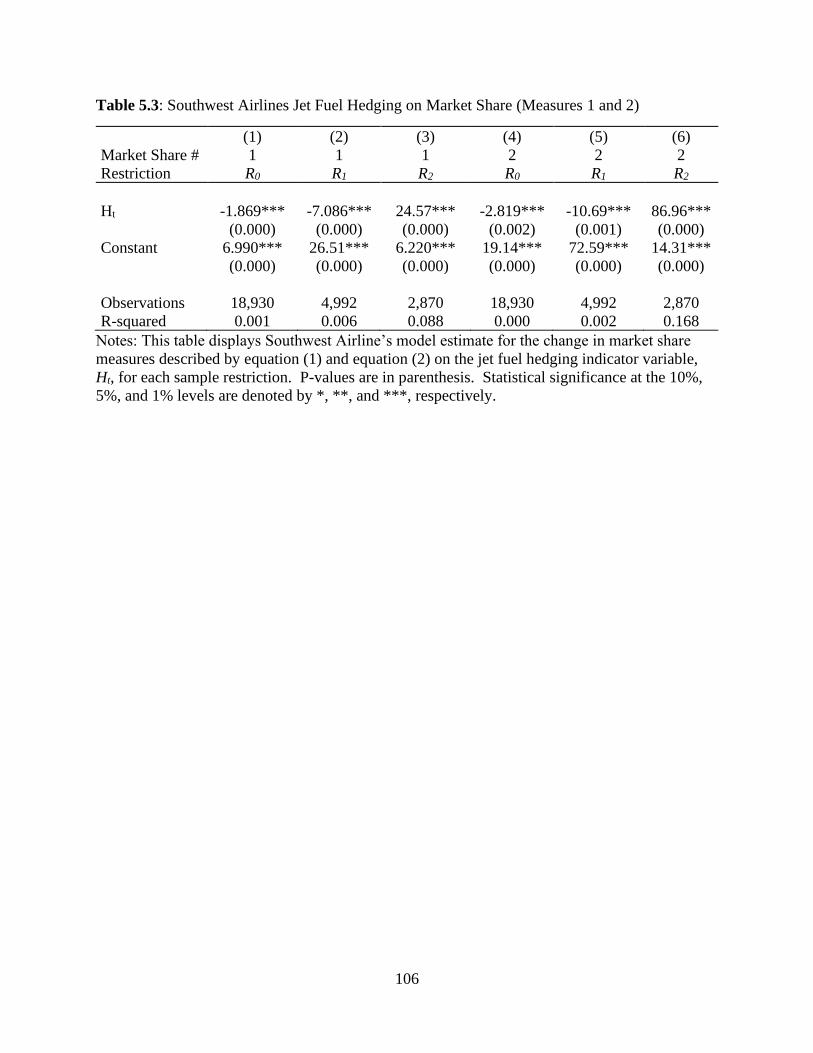
106

Table 5.3: Southwest Airlines Jet Fuel Hedging on Market Share (Measures 1 and 2)

(1) (2) (3) (4) (5) (6)

Market Share # 1 1 1 2 2 2

Restriction R0 R1 R2 R0 R1 R2

Ht -1.869*** -7.086*** 24.57*** -2.819*** -10.69*** 86.96***

(0.000) (0.000) (0.000) (0.002) (0.001) (0.000)

Constant 6.990*** 26.51*** 6.220*** 19.14*** 72.59*** 14.31***

(0.000) (0.000) (0.000) (0.000) (0.000) (0.000)

Observations 18,930 4,992 2,870 18,930 4,992 2,870

R-squared 0.001 0.006 0.088 0.000 0.002 0.168

Notes: This table displays Southwest Airline’s model estimate for the change in market share

measures described by equation (1) and equation (2) on the jet fuel hedging indicator variable,

Ht, for each sample restriction. P-values are in parenthesis. Statistical significance at the 10%,

5%, and 1% levels are denoted by *, **, and ***, respectively.

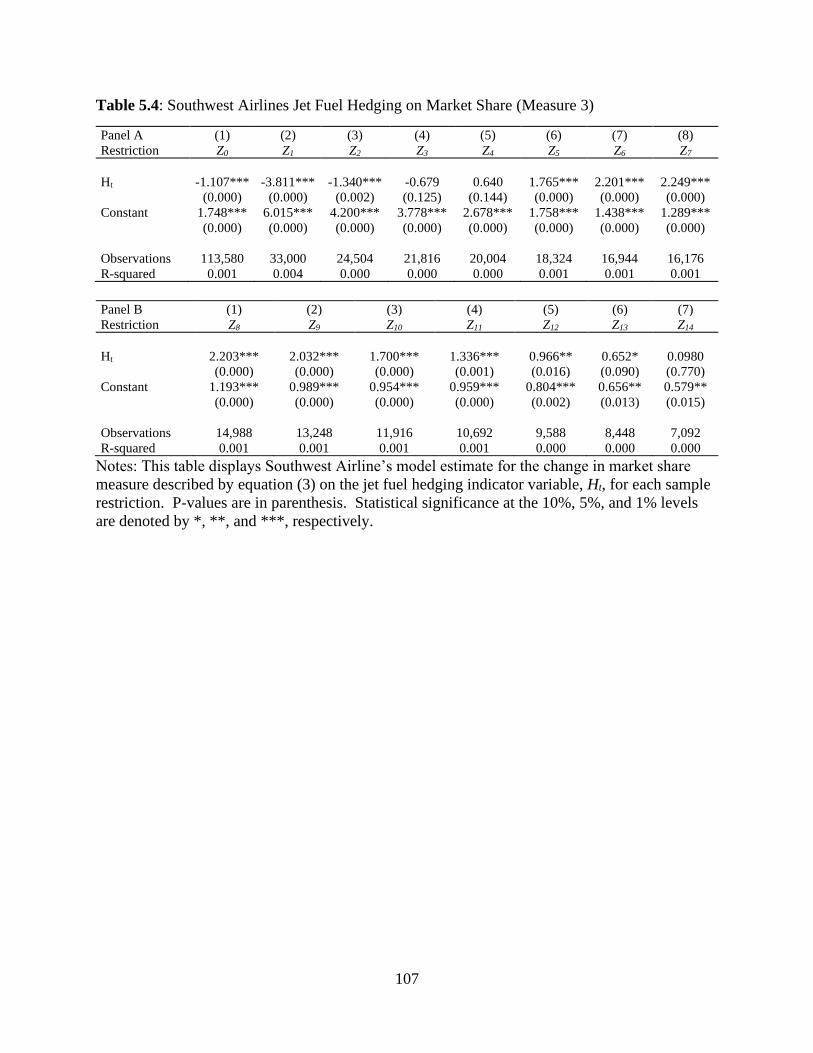
107

Table 5.4: Southwest Airlines Jet Fuel Hedging on Market Share (Measure 3)

Panel A (1) (2) (3) (4) (5) (6) (7) (8)

Restriction Z0 Z1 Z2 Z3 Z4 Z5 Z6 Z7

Ht -1.107*** -3.811*** -1.340*** -0.679 0.640 1.765*** 2.201*** 2.249***

(0.000) (0.000) (0.002) (0.125) (0.144) (0.000) (0.000) (0.000)

Constant 1.748*** 6.015*** 4.200*** 3.778*** 2.678*** 1.758*** 1.438*** 1.289***

(0.000) (0.000) (0.000) (0.000) (0.000) (0.000) (0.000) (0.000)

Observations 113,580 33,000 24,504 21,816 20,004 18,324 16,944 16,176

R-squared 0.001 0.004 0.000 0.000 0.000 0.001 0.001 0.001

Panel B (1) (2) (3) (4) (5) (6) (7)

Restriction Z8 Z9 Z10 Z11 Z12 Z13 Z14

Ht 2.203*** 2.032*** 1.700*** 1.336*** 0.966** 0.652* 0.0980

(0.000) (0.000) (0.000) (0.001) (0.016) (0.090) (0.770)

Constant 1.193*** 0.989*** 0.954*** 0.959*** 0.804*** 0.656** 0.579**

(0.000) (0.000) (0.000) (0.000) (0.002) (0.013) (0.015)

Observations 14,988 13,248 11,916 10,692 9,588 8,448 7,092

R-squared 0.001 0.001 0.001 0.001 0.000 0.000 0.000

Notes: This table displays Southwest Airline’s model estimate for the change in market share

measure described by equation (3) on the jet fuel hedging indicator variable, Ht, for each sample

restriction. P-values are in parenthesis. Statistical significance at the 10%, 5%, and 1% levels

are denoted by *, **, and ***, respectively.

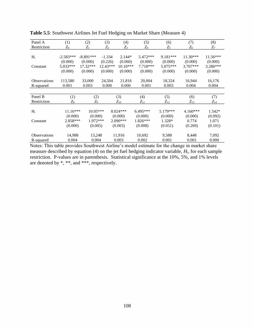
108

Table 5.5: Southwest Airlines Jet Fuel Hedging on Market Share (Measure 4)

Panel A (1) (2) (3) (4) (5) (6) (7) (8)


Ht -2.583*** -8.891*** -1.334 2.144* 5.472*** 9.181*** 11.30*** 11.56***

(0.000) (0.000) (0.226) (0.060) (0.000) (0.000) (0.000) (0.000)

Constant 5.033*** 17.32*** 12.43*** 10.10*** 7.718*** 5.075*** 3.707*** 3.286***

(0.000) (0.000) (0.000) (0.000) (0.000) (0.000) (0.000) (0.000)

Observations 113,580 33,000 24,504 21,816 20,004 18,324 16,944 16,176

R-squared 0.001 0.003 0.000 0.000 0.001 0.003 0.004 0.004

Panel B (1) (2) (3) (4) (5) (6) (7)


Ht 11.16*** 10.05*** 8.024*** 6.495*** 5.179*** 4.160*** 1.542*

(0.000) (0.000) (0.000) (0.000) (0.000) (0.000) (0.092)

Constant 2.858*** 1.972*** 2.090*** 1.826*** 1.328* 0.774 1.071

(0.000) (0.005) (0.003) (0.008) (0.051) (0.269) (0.101)

Observations 14,988 13,248 11,916 10,692 9,588 8,448 7,092

R-squared 0.004 0.004 0.003 0.002 0.001 0.001 0.000

Notes: This table provides Southwest Airline’s model estimate for the change in market share




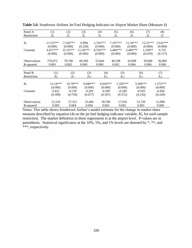
109

Table 5.6: Southwest Airlines Jet Fuel Hedging Indicator on Airport Market Share (Measure 4)

Panel A (1) (2) (3) (4) (5) (6) (7) (8)


Ht -2.113*** -7.243*** -0.894 2.765*** 7.197*** 11.16*** 13.31*** 13.41***

(0.000) (0.000) (0.229) (0.000) (0.000) (0.000) (0.000) (0.000)

Constant 4.471*** 15.33*** 11.26*** 8.702*** 5.466*** 2.485*** 1.258** 0.725

(0.000) (0.000) (0.000) (0.000) (0.000) (0.000) (0.019) (0.157)

Observations 270,072 78,768 60,360 53,844 48,108 43,608 39,060 36,084

R-squared 0.001 0.002 0.000 0.000 0.002 0.004 0.006 0.006

Panel B (1) (2) (3) (4) (5) (6) (7)


Ht 12.14*** 10.78*** 9.040*** 6.916*** 5.102*** 3.506*** 1.373***

(0.000) (0.000) (0.000) (0.000) (0.000) (0.000) (0.009)

Constant 0.421 -0.150 -0.202 -0.269 -0.249 -0.503 -0.456

(0.399) (0.759) (0.677) (0.567) (0.572) (0.210) (0.229)

Observations 31,524 27,312 23,484 20,760 17,916 15,720 12,900

R-squared 0.005 0.004 0.004 0.002 0.002 0.001 0.000

Notes: This table shows Southwest Airline’s model estimate for the change in market share


restriction. The market definition in these regressions is at the airport level. P-values are in


***, respectively.

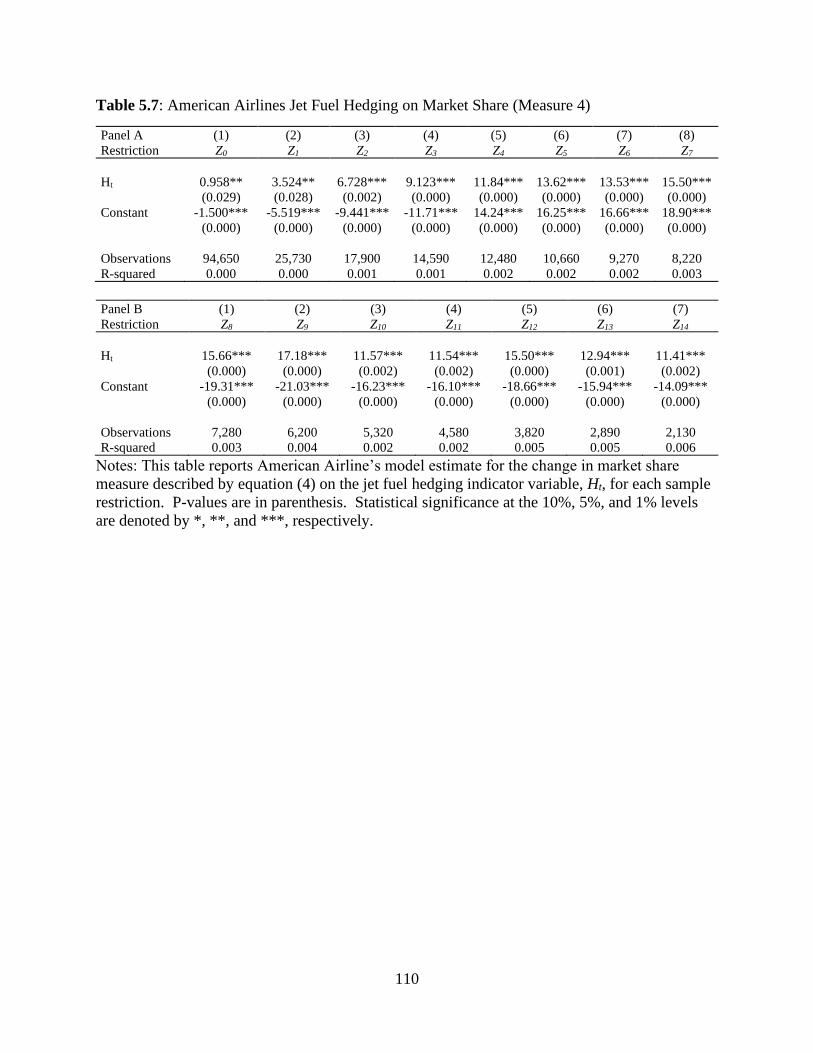
110

Table 5.7: American Airlines Jet Fuel Hedging on Market Share (Measure 4)

Panel A (1) (2) (3) (4) (5) (6) (7) (8)


Ht 0.958** 3.524** 6.728*** 9.123*** 11.84*** 13.62*** 13.53*** 15.50***

(0.029) (0.028) (0.002) (0.000) (0.000) (0.000) (0.000) (0.000)

Constant -1.500*** -5.519*** -9.441*** -11.71*** 14.24*** 16.25*** 16.66*** 18.90***

(0.000) (0.000) (0.000) (0.000) (0.000) (0.000) (0.000) (0.000)

Observations 94,650 25,730 17,900 14,590 12,480 10,660 9,270 8,220

R-squared 0.000 0.000 0.001 0.001 0.002 0.002 0.002 0.003

Panel B (1) (2) (3) (4) (5) (6) (7)


Ht 15.66*** 17.18*** 11.57*** 11.54*** 15.50*** 12.94*** 11.41***

(0.000) (0.000) (0.002) (0.002) (0.000) (0.001) (0.002)

Constant -19.31*** -21.03*** -16.23*** -16.10*** -18.66*** -15.94*** -14.09***

(0.000) (0.000) (0.000) (0.000) (0.000) (0.000) (0.000)

Observations 7,280 6,200 5,320 4,580 3,820 2,890 2,130

R-squared 0.003 0.004 0.002 0.002 0.005 0.005 0.006

Notes: This table reports American Airline’s model estimate for the change in market share




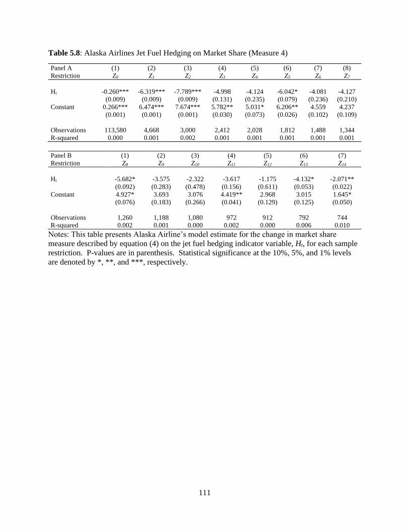
111

Table 5.8: Alaska Airlines Jet Fuel Hedging on Market Share (Measure 4)

Panel A (1) (2) (3) (4) (5) (6) (7) (8)


Ht -0.260*** -6.319*** -7.789*** -4.998 -4.124 -6.042* -4.081 -4.127

(0.009) (0.009) (0.009) (0.131) (0.235) (0.079) (0.236) (0.210)

Constant 0.266*** 6.474*** 7.674*** 5.782** 5.031* 6.206** 4.559 4.237

(0.001) (0.001) (0.001) (0.030) (0.073) (0.026) (0.102) (0.109)

Observations 113,580 4,668 3,000 2,412 2,028 1,812 1,488 1,344

R-squared 0.000 0.001 0.002 0.001 0.001 0.001 0.001 0.001

Panel B (1) (2) (3) (4) (5) (6) (7)


Ht -5.682* -3.575 -2.322 -3.617 -1.175 -4.132* -2.071**

(0.092) (0.283) (0.478) (0.156) (0.611) (0.053) (0.022)

Constant 4.927* 3.693 3.076 4.419** 2.968 3.015 1.645*

(0.076) (0.183) (0.266) (0.041) (0.129) (0.125) (0.050)

Observations 1,260 1,188 1,080 972 912 792 744

R-squared 0.002 0.001 0.000 0.002 0.000 0.006 0.010

Notes: This table presents Alaska Airline’s model estimate for the change in market share




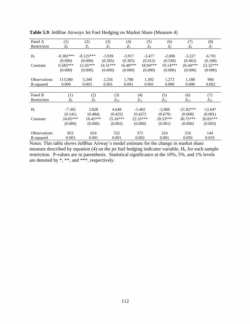
112

Table 5.9: JetBlue Airways Jet Fuel Hedging on Market Share (Measure 4)

Panel A (1) (2) (3) (4) (5) (6) (7) (8)


Ht -0.382*** -8.125*** -3.939 -3.917 -3.477 -2.696 -3.227 -6.701

(0.000) (0.000) (0.265) (0.305) (0.412) (0.530) (0.463) (0.168)

Constant 0.585*** 12.45*** 14.31*** 16.48*** 18.94*** 19.14*** 20.44*** 23.32***

(0.000) (0.000) (0.000) (0.000) (0.000) (0.000) (0.000) (0.000)

Observations 113,580 5,340 2,256 1,788 1,392 1,272 1,188 984

R-squared 0.000 0.003 0.001 0.001 0.001 0.000 0.000 0.002

Panel B (1) (2) (3) (4) (5) (6) (7)


Ht -7.365 3.828 4.648 -5.402 -2.869 -21.82*** -12.64*

(0.141) (0.484) (0.425) (0.427) (0.679) (0.008) (0.081)

Constant 24.05*** 16.45*** 15.16*** 22.35*** 20.53*** 30.75*** 20.83***

(0.000) (0.000) (0.002) (0.000) (0.001) (0.000) (0.003)

Observations 852 624 552 372 324 216 144

R-squared 0.003 0.001 0.001 0.002 0.001 0.050 0.033

Notes: This table shows JetBlue Airway’s model estimate for the change in market share




113

CHAPTER SIX:

HEDGING LITERATURE CONTRIBUTIONS AND FUTURE REASEARCH

6.1 Summary of Dissertation Findings

In the introduction to this dissertation, two contributions to the hedging literature are

emphasized. First, the contribution of the hedging gains and losses variable is discussed in

relation to the seminal Carter, Rogers, and Simkins (2006) study. Smaller contributions in the

reproduction of empirical findings are discussed as well. Second, the contributions to the anti-

trust literature and principal-agent problems in the hedging literature are assessed.

6.1.1 Contributions from Hedging Gains and Losses and Study Reproduction

While the existing theoretical hedging literature explains how hedging can increase value, they

do not attempt to explain the mechanisms for when hedging can increase value. Smith and Stulz

(1985) and Froot, Scharfstein, and Stein (1993) explain how hedging can reduce the variability in

taxes, probability of financial distress, or solve underinvestment by increasing cash flows in low

cash flow states. However, these theories assume that hedging has an expected value of zero.

Hedging can only increase cash flow when hedging contracts are exercised when they have

positive value. Firms that consistently hedge unsuccessfully will not be able to gain value from

those hedges because they do not produce positive cash flow. Hedging gains and losses are

introduced to attempt to explain when hedging will increase firm value and when it will not.

114

Hedging gains and losses variables are added to the firm value models used by Carter,

Rogers, and Simkins (2006) to determine the general effect of jet fuel hedging success on firm

value. Although it was hypothesized that jet fuel hedging gains and losses should have a positive

relationship with firm value, regression results showed a statistically significant negative

correlation. This issue is investigated further by accounting for lease adjustments to important

variables and eliminating realized gains and losses outliers from the sample using a standard box

plot. The majority of the outliers in the data are in 2009 when all hedging airlines suffered

considerable losses from falling jet fuel prices and from Southwest’s hedging success from 2004

to 2008. After removing these outliers from the sample, the realized gains and losses coefficient

became positive but statistically insignificant.

The reproduction of the Carter, Rogers, and Simkins (2006) produces smaller

contributions to the hedging literature. In the literature review chapter, the theoretical hedging

literature has two competing financial constraint theories regarding the determinants of hedging.

Smith and Stulz (1985) propose that financially constrained firms will hedge more to increase

their cash flows in low cash flow states. However, Rampini, Sufi, and Viswanathan (2014)

argue the opposite case, that financially constrained firms are less able to hedge, even if they

want to, because hedging requires collateral that the constrained firms simply do not possess.

Carter, Rogers, and Simkins (2006) find evidence that supports the theory that financially

constrained airlines hedge less, although they claim it is inconsistent with existing theory

(Rampini, Sufi, and Viswanathan (2014) had not yet been published). The reproduction of the

determinants of jet fuel hedging from chapter four offers strong support for the theory that

financially constrained firms hedge less, both in the decision to hedge and the amount hedged.

115

The second minor contribution to the hedging literature is the relationship between

capital expenditures, the hedging premium, and aircraft leases. The Carter, Rogers, and Simkins

(2006) model results find that capital expenditures positively affect the hedging premium. The

results of the replication study from chapter four, however, find a negative and statistically

insignificant coefficient. However, using lease-adjust variables for capital expenditures and

other similarly affected variables produces both positive and statistically significant coefficients.

This suggests that leasing aircraft by airlines plays a significant role in the investments that

airlines may fund through hedging.

6.1.2 Contributions to Principal-agent Problems, Antitrust Concerns, and Hedging

In the literature review of chapter two, a primary assumption in the theoretical literature is that

the investment projects that firms fund with increased cash flow from hedging produces value for

the firm. Tufano (1998), however, suggests that increased cash flow from hedging may result in

a principal-agent problem where managers engage in value-destroying projects. If a project

exists that would benefit a manager at the expense of shareholders or lenders, the manager may

be unable to secure external funding for it. However, hedging may allow the manager to raise

sufficient internal funds to finance the project, bypassing outside scrutiny.

One possible agency issue that may arise from hedging is buying market share, first

introduced by Thomas and Kamp (2006). They propose that managers may believe their

objective is to maximize the market share of the firm, even if their strategy to accomplish this

goal is value destroying to the firm. To gain additional market share, the manager may set price

below cost. Unfortunately, this pricing behavior may be mistaken for predatory pricing and

could subject the firm to costly litigation. Hedging may exacerbate this problem. In chapter one

of the dissertation, it is established that hedging does not lower the cost of the input hedged

116

because the opportunity cost of the input is the value of its next best use, not the price at which it

was obtained. If managers mistakenly believe that successfully hedging lowers the economic

costs to the firm, they may be tempted to pass on the “savings” to consumers in the form of

lower prices, resulting in increased market share.

In chapter five, a preliminary model is formed to test the correlation between successful

jet fuel hedges and changes in market share in the airline industry. Southwest Airlines is used as

the primary airline of interest because of its substantial hedging gains in the early to mid-2000s

followed by losses in 2009 to 2013. Placing multiple restrictions on the markets used in the

regressions, evidence is found suggesting a positive and statistically significant relationship

between successful hedging and increased market share. However, it is emphasized that these

results are preliminary. One must be cautious before declaring that these results indicate buying

market share. As Thomas and Kamp (2006) warn, antitrust officials should be wary of confusing

buying market share behavior with predatory pricing schemes. Predatory pricing, particularly

the attempt to charge monopoly prices after the exit of rivals, is considered anti-competitive

behavior but buying market share is not.

6.2 Future Research

The regressions and models used in this dissertation are by no means exhaustive, particularly for

the relationship between hedging and market share. Additional work is required to distinguish

between increases in market share from entry into new markets or increasing capacity in existing

markets. Controlling for the number of competitors, changes in prices, mergers, among other

concerns is also important. Furthermore, in order to demonstrate that a firm is buying market

share, it must be shown that the airline is achieving increased market share while pricing below

cost. A significant econometric concern is the endogenous relationship between price and

117

market share. That is, while lowering prices may increase market share, increases in market

share may allow firms to raise price. Care must be taken to identify strong instrumental

variables to control for endogeneity.

Buying market share is also likely to occur at individual markets rather than across all

possible markets where an airline operates. As mentioned in chapter five, the predatory pricing

case against American Airlines in 2001 only involved four markets. Testing for buying market

share may require identifying markets where it is more likely, possibly where larger airlines are

competing with smaller carriers who could not sustain operations in a low-price environment.

118

REFERENCES

Alaska Air Group, Inc. 2008. Form 10-K (annual report). From SEC EDGAR Database.

Accessed August 18, 2018.

Alaska Air Group, Inc. 2009. Form 10-K (annual report). From SEC EDGAR Database.


Allayannis, George, and James P. Weston. “The Use of Foreign Currency Derivatives and Firm

Market Value.” The Review of Financial Studies 14 (2001): 243–276.

AMR Corporation 2002. Form 10-K (annual report). From SEC EDGAR Database.

Accessed February 14, 2019.

AMR Corporation 2008. Form 10-K (annual report). From SEC EDGAR Database.

Accessed February 14, 2019.

Belghitar, Yacine, Ephraim Clark, and Amrit Judge. “The Value Effects of Foreign Currency and

Interest Rate Hedging: The UK Evidence.” International Journal of Business 13 (2008):

43-60.

Carter, David A., Daniel A. Rogers, and Betty J. Simkins. “Does hedging affect firm value?

Evidence from the US airline industry.” Financial Management 35 (2006): 53–86.

Carter, David A., Daniel A. Rogers, Betty J. Simkins, Stephen D. Treanor. “A Review of the

Literature on Commodity Risk Management.” Journal of Commodity Markets 8 (2017):

1-17.

Chung, Kee H. and Stephen W. Pruitt. “A Simple Approximation of Tobin’s Q.” Financial

Management 23 (1994): 70-74.

“City Pairs.” Federal Aviation Administration. Last modified January 30, 2018. Accessed

August 14, 2018. https://www.faa.gov/nextgen/snapshots/airportpairs/.

“Code Share Fact Sheet.” U.S. General Services Administration. Last reviewed April 23, 2018.

https://www.gsa.gov/travel/plan-book/transportation-airfare-rates-pov-rates-etc/airfare-

rates-city-pairs-programs/resource-library/code-share-fact-sheet.

Damodaran, A., 2002. Investment Valuation: Tools and Techniques for Determining the Value of

any Asset, 2nd Ed., John Wiley & Sons, New York.

https://www.faa.gov/nextgen/snapshots/airportpairs/

https://www.gsa.gov/travel/plan-book/transportation-airfare-rates-pov-rates-etc/airfare-%20%20%20%20%20%20%20%20%20%20%20rates-city-pairs-programs/resource-library/code-share-fact-sheet

https://www.gsa.gov/travel/plan-book/transportation-airfare-rates-pov-rates-etc/airfare-%20%20%20%20%20%20%20%20%20%20%20rates-city-pairs-programs/resource-library/code-share-fact-sheet

119

“Data Profile: Air Carrier Statistics (Form 41 Traffic) – All Carriers.” Bureau of Transportation

Statistics. Accessed August 15, 2018.

https://www.transtats.bts.gov/DatabaseInfo.asp?DB_ID=111.

Delta Air Lines, Inc. 1999. Form 10-K (annual report). From SEC EDGAR Database.


Froot, Kenneth A., David S. Scharfstein, and Jeremy C. Stein. “Risk Management: Coordinating

Investment and Financing Policies,” The Journal of Finance 48 (1993): 1629-1658.

Graham, John R. and Daniel A. Rogers. “Do Firms Hedge in Response to Tax Incentives?” The

Journal of Finance 57 (2002): 815-839.

Haushalter, David G. “Financing Policy, Basis Risk, and Corporate Hedging: Evidence from Oil

and Gas Producers.” The Journal of Finance 55 (2000): 107-152.

Jin, Yanbo and Phillipe Jorion. “Firm Value and Hedging: Evidence from U.S. Oil and Gas

Producers.” Journal of Finance 61 (2006): 893–919.

Lundy, James. “DOT T-100 and O&D Survey Data Overview.” Campbell-Hill Aviation Group,

LLC. January 2016. https://www.aci-na.org/sites/default/files/lundy-pbi.pdf.

Modigliani, Franco and Merton H. Miller. “The Cost of Capital, Corporation Finance and the

Theory of Investment.” The American Economic Review 48 (1958): 261-297.

Morrell, Peter and William Swan. “Airline Jet Fuel Hedging: Theory and Practice.”

Transportation Reviews 26 (2006): 713-730.

Rampini, Adriano A., Amir Sufi, and S. Viswanathan. “Dynamic Risk Management.”

Journal of Financial Economics 111 (2014): 271-296.

Smith, Clifford W. and René M. Stulz. “The Determinants of Firms’ Hedging Policies,” Journal

of Financial and Quantitative Analysis 20 (1985): 391-405.

Southwest Airlines Co. 2001. Form 10-K (annual report). From SEC EDGAR Database.






Thomas, Christopher R. and Bradley P. Kamp. “Buying Market Share: Agency Problem or

Predatory Pricing?” Review of Law and Economics 2 (2006): 1-24.

https://www.transtats.bts.gov/DatabaseInfo.asp?DB_ID=111

https://www.aci-na.org/sites/default/files/lundy-pbi.pdf

120

Treanor, Stephen, Daniel A. Rogers, David A. Carter, Betty J. Simkins. “Does Operational and

Financial Hedging Reduce Exposure? Evidence from the U.S. Airline Industry.” The

Financial Review 49 (2014a): 149-172.

Treanor, Stephen, Betty J. Simkins, Daniel A. Rogers, David A. Carter. “Exposure, Hedging,

and Value: New Evidence from the U.S. Airline Industry.” International Review of

Financial Analysis 34 (2014b): 200-211.

Tufano, Peter. “Who Manages Risk? An Empirical Examination of Risk Management

Practices in the Gold Mining Industry.” The Journal of Finance 51 (1996): 1097-1137.

Tufano, Peter. “Agency Costs of Corporate Risk Management.” Financial Management 27

(1998): 67-77.

United Continental Holdings, Inc. 2014. Form 10-K (annual report). From SEC EDGAR

Database. Accessed August 18, 2018.

Vasigh, Bijan, Kenneth Fleming, and Barry Humphreys. Foundations of Airline Finance:

Methodology and Practice. New York: Routledge, 2014.