An Optimal Solution to a General Dynamic Jet FuelHedging Problem

Juliana M. NascimentoWarren B. Powell

Department of Operations Research and Financial EngineeringPrinceton University

February 11, 2008

Abstract

We propose a dynamic hedging strategy for jet fuel which strikes a balance between hedgingagainst jumps in the price of jet fuel and placing bets that the price will rise, lowering theoverall cost of jet fuel. We model the commodity price using an unobservable two-factormodel that allows mean-reversion in short-term prices and uncertainty in the equilibriumlevel to which prices revert. We combine dynamic programming and Kalman filter estimationto obtain an optimal policy that minimizes the expected costs while keeping the variance atlow levels.

1 Introduction

Jet fuel costs account for a large portion of an airline’s operating expenses and when fuel

prices rise dramatically, airlines cannot pass all of the costs on to their customers (Zea

(2004)). Also, it is almost impossible for an airline to stock large amounts of jet fuel, due

to financing and storage costs. Therefore, an effective strategy for airlines is to hedge fuel

costs to avoid huge swings in expenses. As pointed out in Morrell & Swan (2006), hedging

may still help reduce volatility in earnings by moving profits from one quarter to another.

Despite its potential, jet fuel hedging remains a largely unused strategy. Some executives

claimed that risk would be present regardless of whether they hedged or not. Furthermore,

they claimed that hedging was not a core competency and as long as competitors were not

hedged, it was a level playing field (Zea (2004)). But low-cost airlines such as Southwest

(Carter et al (2004)) have benefited considerably from an aggressive hedging strategy1. It

was shown in Carter et al. (2006) that there is a hedging premium for stocks of airlines using

derivatives to hedge jet fuel exposure. The authors also show that hedging allows airlines to

take advantage of investment opportunities in times of high commodity prices.

Both over-the-counter (OTC) and exchange-traded derivatives can be used for hedging.

Nevertheless, a perfect hedge is practically impossible. OTC contracts on jet fuel include

options, collar structures and swaps. Even though the ability to customize these derivatives

is a big plus, there are several disadvantages associated with them. First, they are rather

illiquid, making them very expensive. Second, there is counter-party risk. Finally, they are

not available in quantities sufficient to hedge all of an airline’s jet fuel consumption.

On the other hand, exchange-traded derivatives are more liquid and eliminate counter-

party risk. However, these contracts are not available in the U.S. for jet fuel. Therefore,

contracts on commodities that have a high price correlation with jet fuel must be used for

hedging. Heating and crude oil are usually the commodities of choice, since jet fuel shares

similar characteristics with the first and is refined from the second. Finally, as exchange-

traded contracts for hedging jet fuel costs are standardized (inflexible) and are based on

1See the article An Airline Shrugs at Oil Prices at The New York Times on November 29, 2007.

1

a different underlying commodity, the associated basis risk is larger compared with OTC

derivatives.

In this paper, we derive a dynamic strategy based on exchange-traded futures contracts

on heating or crude oil to hedge jet fuel demand that will occur at time T . The hedging

policy should maximize

IE

[∑t∈T

e−rtUt(Wt, Rt, Xt)

], (1)

where T is the set of trading times prior to T , r is the risk-free interest rate, Wt is the

information available up until time t, Rt is the number of futures contracts standing at t

and Xt is the policy. The information vector Wt includes the spot price of oil and fuel. It

also includes the current and the previous (last trading date) price of the future contract

maturing a month after T . The dynamic policy Xt determines the trading decision taken

at t. Moreover, Ut(Wt, Rt, Xt) is the utility function under consideration, where both risk

and return play a role. A prospective test on the hedge effectiveness is also taken into

account. The relative importance of risk versus the cost of the jet fuel is defined by a weight

determined by the investor to accommodate his preferences.

The most widely used hedging strategy considering futures contracts is the dynamic

minimum variance optimal hedge ratio (OHRt) given by

OHRt =σtFC

σ2tF

, (2)

where, in the jet fuel case, σtFC is the covariance between the price of the future contract

and the spot price of fuel and σ2tF is the variance of the price of the future contract. Both

the covariance and the variance are computed using information available up until time

t. Almost all the research on hedging focuses on minimizing the variance of the deviation

between jet fuel and the hedge (Lien & Tse (2002)), ignoring other dimensions such as the

cost of the jet fuel.

We differ from this conventional approach since we focus on deriving and computing an

optimal dynamic hedging strategy for a more general utility which considers not only the

variance of the deviation between jet fuel and the hedge, but also the expected cost of the

2

jet fuel. Thus, depending on the weight that we put on the variance, we are willing to accept

higher risk if it lowers the expected cost of the jet fuel. We use dynamic programming to

derive the optimal strategy.

To model the oil spot price we use the two-factor model proposed in Schwartz & Smith

(2000). This model allows mean-reversion in short-term prices and uncertainty in the equi-

librium level to which prices revert. To model the relationship between the oil spot price

and the fuel spot price, we use the time varying regression (TVR) model discussed in Bos &

Gould (2007). In this model, the correlation between the two prices varies with time and is

represented by a martingale. However, the two factors in the oil spot price model can not

be directly observed and their parameters are not known. The same is true for the mar-

tingale and the associated parameters. We use the Kalman filter and maximum likelihood

estimation to recursively estimate the parameters and the processes themselves based on

observations of spot and future prices for oil and spot prices for fuel.

The main contribution of this paper is the derivation of an optimal dynamic hedging

strategy with respect to a utility function that allows the investor to control the relative

importance of risk mitigation and speculation. Even though the curse of dimensionality of

dynamic programming could have prevented us from actually computing such policy, we

show that the corresponding optimal value function is quadratic in the number of contracts

standing. We also show that computing the optimal policy depends only on our ability to

compute the expected values involving the future contract prices and the spot prices of fuel

and oil. The two-factor (Schwartz & Smith (2000)) and the TVR (Bos & Gould (2007))

models allow us to obtain accurate estimates of the expected values. Using historical price

data, we demonstrate the relative performance of our policy over popular competing policies

as a function of the weight on risk. For certain weight ranges, we show that our policy

dominates other policies by producing hedges with lower risk as well as lower average fuel

cost.

3

2 Literature Review on Hedging

There is an extensive literature on the use of derivatives to hedge a particular risk in the

future (Lien & Tse (2002)). The risk might be associated to a foreign exchange rate, to a

commodity price or to the level of the stock market to name a few. Jet fuel hedging is a

special case, with its own characteristics. The best-known hedging strategy using futures

contracts (Hull (2000)) is the minimum variance optimal hedge ratio (OHR), which is the

ratio of the size of the position taken in future contracts to the size of the exposure. The

OHR is usually used as a benchmark. In Cecchetti et al. (1988) the authors applied the

two-asset portfolio model to determine that

OHR =σFC

σ2F

, (3)

where, as described in the introduction, σFC is the covariance between the price of the

future contract and the spot price of fuel and σ2F is the variance of the price of the future

contract. This is a static strategy called hedge-and-forget. It assumes that the hedge position

is not going to be changed over the duration of the hedge. The choice of the model and the

technique to estimate the covariance and the variance is the subject of several papers. For

example, in Tunaru & Tan (2002), the authors use different regression models.

On the other hand, a large literature initiated by Baillie & Myers (1991) allows the min-

imum variance hedge ratio to vary over time. The dynamic version is given by (2). A short

review on estimating the time-dependent (co)variances can be found in Chen et al. (2003).

Most papers estimate dynamic hedge ratios (Bos & Gould (2007)) using either the (G)ARCH

framework of Engle (1982) and Bollerslev (1986) or the stochastic volatility approach, intro-

duced into the econometric literature by Harvey et al. (1994) and Jacquier et al. (1994). The

required estimations are obtained either using a (quasi) maximum likelihood or a Bayesian

approach.

Combining the GARCH and the dynamic programming frameworks to construct a dy-

namic strategy has been explored before. In Haigh & Holt (2002), the authors combined the

two to hedge the risk associated with purchasing commodities for use in food manufactur-

ing. Their objective was to minimize the variance of the total terminal cost. The resulting

4

optimal policy is very similar to the dynamic OHR. The only difference, for time period t, is

that the variance in the denominator of (2) is multiplied by rT−t, where r is a discount factor

and T is the end of the hedge period. Our paper differs from this work since we consider a

more complex utility function, yielding a strategy that allows for a tradeoff between hedging

and speculation according to the investor’s preferences.

Both the static and the dynamic hedge ratios are optimum when the objective is to

minimize the risk, not to maximize expected utility, which also depends on expected return.

As pointed out by Cecchetti et al. (1988), only a totally risk averse investor can make an

optimal hedging decision without taking the impact on both risk and return into account.

Value at risk (VaR) is another metric that has been considered in the literature. The static

and dynamic zero-VaR hedge ratios for futures contracts were discussed in Hung et al. (2005)

and Lee & Hung (2007), respectively.

A different line of hedging research pursued in the economics literature focuses on con-

structing a self-financing dynamic portfolio strategy that most closely approximates a given

payoff function at a future maturity date. For example, in Heath et al. (2001), Laurent

& Pham (1999) and Bertsimas et al. (2001) the authors approach the problem considering

minimizing a mean variance or quadratic utility function of the given payoff. They also

consider a class of stochastic volatility models in an incomplete financial market. The last

two papers use dynamic programming to achieve their goal.

3 The Hedging Setup

We establish the notation and the assumptions we will use for the rest of the paper. The

demand for jet fuel occurs at time T . It is assumed to be known and is denoted by d. The

hedging is done using future contracts based either on heating or crude oil and the investor

has N trading opportunities prior to T . In practice, to avoid actual delivery of the hedging

commodity (heating or crude oil), the maturity of the future contract is typically chosen to

be one month after T . The set of trading dates is given by T = {tN , . . . , t1}. Without loss of

generality, we assume that the time between two consecutive trading dates is constant and

5

is equal to ∆. We also assume that the time between the last trading date t1 and T is also

equal to ∆. We assume the risk-free interest rate is known and is equal to r.

The price of a future contract at t maturing at t′ is denoted by Ftt′ . Moreover, the spot

price of oil and the spot price of fuel at t are denoted, respectively, by P ot and P f

t . All of

them are in dollars per barrel. The vector Wt = (P ot , P f

t , Ftt′ , Ft−∆,t′), called the information

vector, contains the exogenous information relevant to the hedging problem. We discuss in

section 6 the models governing the underlying processes.

We denote by Rt the number of future contracts standing prior to the trading decision at

time t, denoted by xt. Clearly, Rt+∆ = Rt +xt. In the beginning of the hedging period there

are no contracts standing, i.e., RtN = 0. Moreover, xT = −RT , indicating that the future

position is closed at the end of the hedging period. For t ∈ T , we impose that xt must be

greater than or equal to −Rt, so that the number of standing contracts is never negative.

We say that (Wt, Rt) represents the state of our system.

The cash flow at each time period t ∈ T ∪ {T} is given by

Cflt (Wt, Rt, xt) = 103

((Ftt′ − Ft−∆,t′)Rt − P f

T d1{t=T}

), (4)

as the future contract price Ftt′ is in dollars per barrel and the size of each contract is 103

barrels. Thus, by the end of the hedging period, the realized cost per barrel is given by

Cπ =∑

t∈T ∪{T}

er(T−t)Cflt (Wt, Rt, X

πt )

d, (5)

where Xπt is the policy/hedging strategy that determines the trading decision xt at t.

4 Hedging Strategies

Before we introduce our policy, we discuss in this section four popular hedging strategies

that we use as a comparison in our computational experiments.

• No-Hedge: The simplest strategy is to not hedge at all. Using this strategy xt = 0

for t ∈ T ∪ {T}. Clearly, the realized cost per barrel is CNo-hedge = −P fT .

6

• Naive: This strategy is also very straightforward. We buy d future contracts in

the beginning of the hedge period and close the position at T . That is, xtN = d,

xtN−1= · · · = xt1 = 0 and xT = −d. In this case, the realized cost per barrel is

CNaive = (FTt′ − FtN ,t′erN∆)− P f

T .

• Optimal hedge ratio (OHR): Also known as the hedge-and-forget ratio, this is the

basic strategy that determines the number of contracts to purchase at the beginning

of the hedging period based on the ratio given by the covariance between the fuel spot

price and the future contract price and the variance of the future contract price. It is

optimal when the utility function considered is the variance of the cash flow. We have

that

xtN =Cov(P f

T , FTt′ − FtN ,t′)

V ar[FTt′ − FtN ,t′ ]d, xtN−1

= · · · = xt1 = 0 and xT = −xtN .

• Dynamic hedge ratio (OHRt): This is the dynamic version of the previous strategy.

At each trading opportunity, new information has become available resulting in an

updated covariance and variance. The number of contracts standing is thus rebalanced

to reflect the current ratio. In this case, for t ∈ T , we have that

xt =Covt(P

fT , FTt′ − Ftt′)

V art[FTt′ − FtN ,t′ ]d−Rt−∆ and xT = −xt1 = −Rt1 .

where the subscript t indicates that the covariance and the variance are conditional on

the information up until time period t.

5 Optimal Dynamic Hedging

We now propose our hedging strategy. We start by defining the utility function under

consideration. For t ∈ T ∪ {T}, our utility function is given by

Ut(Wt, Rt, xt) = Cflt (Wt, Rt)− uvol

(Cfl

t (Wt, Rt))2

+ 103e−r(T−t)IEt

[(FTt′ − Ftt′)(Rt + xt)− P f

T d]

(6)

− 106e−r(T−t)uvolIEt

[((FTt′ − Ftt′)(Rt + xt)− P f

T d)2

].

7

The first term represents the return, while the second term represents its volatility. Moreover,

we perform a prospective test on the hedge effectiveness, represented by the last two terms.

They measure in terms of return and risk how well the strategy would do by the end of the

hedging period, if we were to stop trading at t. Clearly, the test is performed using the price

information and the expected values we have available at t. Remember that the rationale

behind the 103 and 106 coefficients is that the future contract price Ftt′ is in dollars per barrel

and the size of each contract is 103 barrels. We point out that uvol > 0 is the investor-defined

weight indicating how much risk he is willing to take.

Our objective is to construct a policy Xt(Wt, Rt), which is a function of the current state

(Wt, Rt), that maximizes (1). The trading decision xt is determined by this policy.

We solve the problem using dynamic programming. In this framework, the downstream

effects of the decision xt taken at time t is determined by the optimal value function at

the next time period t + ∆. The value functions are determined recursively in a backward

fashion. At the end of the hedging period T , it is clear that VT (WT , RT ) = UT (WT , RT ,−RT ).

Recursively, for t ∈ T , we have that

Vt(Wt, Rt) = max−Rt≤xt

IEt

[Ut(Wt, Rt, xt) + e−r∆Vt+∆(Wt+∆, Rt + xt)

]. (7)

The resulting optimal policy and the corresponding optimal value function are described

in the next theorem. We emphasize that the classic curse of dimensionality associated with

dynamic programming formulations could have been an issue here, however Theorem 1 shows

that the optimal value functions are quadratic in the number of future contracts standing.

Computing the optimal policy only depends on our ability to compute the expected values

involved.

Theorem 1. For t ∈ T , the optimal policy with respect to the utility function described in

(6) is given by

X∗t (Wt, Rt) = max

(−Rt, X

∗,tempt (Wt, Rt)

), (8)

8

where

X∗,tempt (Wt, Rt) =

IEt

[e−r(T−t)(FTt′ − Ftt′) + e−r∆(Ft+∆,t′ − Ftt′)

]2× 103uvolIEt [e−r(T−t)(FTt′ − Ftt′)2 + e−r∆(Ft+∆,t′ − Ftt′)2]

+IEt

[e−r(T−t)(FTt′ − Ftt′)P

fT + e−r∆(FTt′ − Ftt′)P

fT 1{t=t1}

]2× 103uvolIEt [e−r(T−t)(FTt′ − Ftt′)2 + e−r∆(Ft+∆,t′ − Ftt′)2]

d−Rt.

The corresponding optimal value function is a concave quadratic function of Rt given by

Vt(Wt, Rt) = −106uvol(Ftt′ − Ft−∆,t′)2R2

t + 103(Ftt′ − Ft−∆,t′)Rt + v0t (Wt), (9)

where v0t (Wt) is a term independent of Rt.

Proof. The proof is by backward induction on t. We start with the base case t = t1. By

definition, for t = t1,

Vt(Wt, Rt) = max−Rt≤xt

Ut(Wt, Rt, xt) + e−r∆IEt [UT (WT , Rt + xt,−(Rt + xt))] . (10)

Plugging in (6) and ignoring the terms that are independent of xt, it turns out that we have

to maximize the concave and quadratic function of xt given by

ft(xt) = −106uvolIEt

[e−r(T−t)(FTt′ − Ftt′)

2 + e−r∆(Ft+∆,t′ − Ftt′)2]x2

t

+ 103IEt

[e−r(T−t)(FTt′ − Ftt′) + e−r∆(Ft+∆,t′ − Ftt′)

]xt

+ 103IEt

[e−r(T−t)(FTt′ − Ftt′)P

fT d + e−r∆(FTt′ − Ftt′)P

fT d

]xt

− 2× 106uvolIEt

[e−r(T−t)(FTt′ − Ftt′)

2R + e−r∆(Ft+∆,t′ − Ftt′)2R

]xt,

subject to xt ≥ −Rt.

It is easy to see that the solution to the unconstrained maximization problem is the

expression for X∗,tempt (Wt, Rt). The optimal policy is thus obtained as we have to enforce

the lower bound −Rt. The quadratic value function is obtained by plugging in the expression

for the optimal policy in (10), concluding the base case. The induction step assumes that

(9) holds for t ∈ T . The proof that (8) and (9) hold for t−∆ follows the same reasoning as

the base case. Namely, we use (7) and the induction hypothesis to derive the concave and

quadratic function of xt−∆ that has to be maximized. The optimal policy and the resulting

value function will follow from there. �

9

We finish this section by noting that the terms on the policy discounted by e−r(T−t) are

due to the prospective test, while the terms discounted by e−r∆ are due to the effect the

decision at t will have at the next trading opportunity.

6 The Price Models

We present the models governing the price processes and we derive expressions to the ex-

pected values involved in our optimal policy. Our model choice intended to achieve a good

tradeoff between accurately describing the stochastic evolution of the processes and providing

analytical expressions for the expected values of interest.

Following the model introduced in Schwartz & Smith (2000), the log of the oil spot price

is decomposed into two stochastic factors, namely

ln(P ot ) = χt + ξt,

where χt represents a short-term deviation in prices that are not expected to persist. On

the other hand, ξt represents the long-term equilibrium price level. Changes in ξt indicates

fundamental changes that are expected to persist.

The short-term deviations are assumed to follow a Ornstein-Uhlenbeck (OU) process

dχt = −κχtdt + σχdzχ,

while the equilibrium level is assumed to follow a Brownian motion process

dξt = µξdt + σξdzξ.

In these models, dzχ and dzξ are correlated increments of standard Brownian motion pro-

cesses with dzχdzξ = ρχξdt. Moreover, κ describes the rate at which the short-term deviations

are expected to disappear. In addition, we let σχ and σξ be the short term and equilibrium

volatilities. Finally, µξ is the equilibrium drift rate.

For t′ > t, it was shown in Schwartz & Smith (2000) that conditioned on the information

up to time t, (χt′ , ξt′) are jointly normally distributed with mean vector and covariance

10

matrix:

IEt[(χt′ , ξt′)] =[e−κ(t′−t)χt, ξt + µξ(t

′ − t)]

(11)

Ct[(χt′ , ξt′)] =

(1− e−2κ(t′−t))σ2χ/2κ (1− e−κ(t′−t))ρχξσχσξ/κ

(1− e−κ(t′−t))ρχξσχσξ/κ σ2ξ (t

′ − t)

. (12)

We thus have that the logarithm of the oil spot price at t′, given (χt, ξt), is normally dis-

tributed with mean µoiltt′ and variance σ2,oil

tt′ , where

µoiltt′ = e−κ(t′−t)χt + ξt + µξ(t

′ − t) (13)

σ2,oiltt′ = (1− e−2κ(t′−t))

σ2χ

2κ+ σ2

ξ (t′ − t) + 2(1− e−κ(t′−t))

ρχξσχσξ

κ. (14)

Therefore, given (χt, ξt), P ot′ is log-normally distributed with mean and variance

IEt[Pot′ ] = eµoil

tt′+.5σ2,oil

tt′ (15)

V art[Pot′ ] =

(eσ2,oil

tt′ − 1)

e2µoiltt′+σ2,oil

tt′ . (16)

We now discuss the relationship between the spot price of oil and the spot price of fuel.

We consider the time varying regression (TVR) model presented in Bos & Gould (2007).

The results in that paper indicate that the TVR is a good tradeoff between having a simple

model and obtaining good results for the correlation between a pair of prices. In the TVR

model, the dynamics between the two spot prices are given by the equations

dβt = σβdzβ (17)

P ft = α + βtP

ot + εt, (18)

where σβ is the process volatility and dzβ is an increment of a standard Brownian motion

process, which is independent of dzχ and dzξ. We have that βt is a martingale representing

the correlation between the prices. Moreover, α is a constant and εt is a noise term that is

normally distributed with mean zero and variance σ2ε . Clearly, we have that

IEt[PfT ] = α + βtIEt[P

oT ], (19)

where IEt[PoT ] is given by (15) replacing t′ with T .

11

Using the risk-neutral valuation framework (Duffie (1992)), future prices are equal to the

expected future spot price under the risk-neutral measure. Therefore, we now focus on the

risk-neutral processes governing the oil spot price.

As before, the short-term deviation follows a OU process and the equilibrium level follows

a Brownian motion process, given, respectively, by

dχt = (−κχt − λχ)dt + σχdz∗χ (20)

dξt = (µξ − λξ)dt + σξdz∗ξ , (21)

where, again, dz∗χ and dz∗ξ are increments of standard Brownian motion processes under the

risk-neutral measure with dz∗χdz∗ξ = ρχξdt. Here, λχ and λξ are, respectively, the short term

and the equilibrium risk premiums. Note that the risk-neutral OU process reverts to −λχ/κ

(instead of 0 in the real world OU process) and the risk-neutral Brownian motion drift is

µ∗ξ ≡ µξ − λξ (instead of µξ).

Hence, under the risk-neutral measure, conditioned on the information up to time t,

(χt′ , ξt′) are jointly normally distributed with mean vector and covariance matrix

IE∗t [(χt′ , ξt′)] =[e−κ(t′−t)χt −

(1− e−κ(t′−t)

)λχ/κ, ξt + µ∗ξ(t

′ − t)]

C∗t [(χt′ , ξt′)] = Ct[(χt′ , ξt′)].

We use asterisks to denote expectations and (co)variance taken with respect to the risk

neutral measure.

We conclude that given (χt, ξt), the logarithm of the spot price at t′ under the risk neutral

measure is normally distributed with mean and variance

IE∗t [ln(P ot′)] = e−κ(t′−t)χt −

(1− e−κ(t′−t)

)λχ/κ + ξt + µ∗ξ(t

′ − t)

V ar∗t [ln(P ot′)] = σ2,oil

tt′ .

Since, by definition, FTt′ = IE∗T [P ot′ ], we have that

ln(FTt′) = ln(IE∗T [P ot′ ]) = IE∗T [ln(P o

t′)] +1

2V ar∗T [ln(P o

t′)]

= e−κ(t′−T )χT + ξT + A(t′ − T ), (22)

12

where A(t) = µ∗ξt− (1− e−κt)λχ

κ+ 1

2

((1− e−2κt)

σ2χ

2κ+ σ2

ξ t + 2(1− e−κt)ρχξσχσξ

κ

).

We compute some expectations involving P fT and FTt′ . We start with the conditional

expected value and variance of ln(FTt′) at t, denoted by µfutt,T t′ and σ2,fut

t,T t′ , respectively. We

have that

µfutt,T t′ = IEt

[e−κ(t′−T )χT + ξT + A(t′ − T )

]= e−κ(t′−t)χt + ξt + µξ(T − t) + A(t′ − T )

and

σ2,futt,T t′ = V art

[e−κ(t′−T )χT + ξT + A(t′ − T )

]= e−2κ(t′−T )

(1− e−2κ(T−t)

) σ2χ

2κ+ σ2

ξ (T − t) + 2e−κ(t′−t)(1− e−2κ(T−t)

) ρχξσχσξ

κ.

Therefore, as with the oil spot price, conditioned on the information until t, FTt′ is log-

normally distributed with mean and variance

IEt[FTt′ ] = eµfut

t,T t′+.5σ2,fut

t,T t′ (23)

V art[FTt′ ] =(e

σ2,fut

t,T t′ − 1)

e2µfut

t,T t′+σ2,fut

t,T t′ . (24)

The conditional expectation of the product between the spot and the future contract

price for oil at T is our next computation. We have that

P oT FTt′ = exp (χT + ξT ) exp

(e−κ(t′−T )χT + ξT + A(t′ − T )

)= exp

((1 + e−κ(t′−T )

)χT + 2ξT + A(t′ − T )

).

Hence,

IEt [P oT FTt′ ] = exp

[(1 + e−κ(t′−T )

)IEt[χT ] + 2IEt[ξT ] + A(t′ − T )

+1

2

((1 + e−κ(t′−T )

)2

V art[χT ] + 4V art[ξT ]

)+ 2

(1 + e−κ(t′−T )

)Covt(χT , ξT )

].

We close the section pointing out that

IEt

[P f

T FTt′

]= IEt [(α + βT P o

T + εT )FTt′ ] = αIEt [FTt′ ] + βtIEt [P oT FTt′ ] ,

as βT is independent of P oT FTt′ , εT is independent of FTt′ , βt is a martingale and IEt [εT ] = 0.

13

7 Processes and Parameter Estimation

The processes χt and ξt are unobservable, as we only have access to future and spot prices.

The same is true for βt, the process governing the correlation between the oil and fuel spot

prices. Moreover, the parameters for the oil spot price θ = (κ, σχ, σξ, ρχξ, λχ, µ∗ξ , µξ) and the

parameters α, σ2β and σ2

η for the relationship between oil and fuel prices are also unknown.

We thus combine Kalman filter (KF) and maximum likelihood estimation to obtain estimates

for these processes and parameters.

The Kalman filter is a recursive procedure to compute estimates of the unobserved pro-

cesses based on observations, in our case of future and spot prices, that are driven by these

processes. It generates updated posterior distributions for the considered processes following

the Bayes rule. As is the norm in a Bayesian setting, a prior distribution for the initial value

of the unobserved processes is required. One way to view Kalman filtering is to think of it

as an updating procedure that consists of forming a preliminary guess about the unobserved

processes and then adding a correction to this guess, the correction being determined by how

well the guess has performed in predicting the next observation.

We first discuss the estimation of the processes χt and ξt and the corresponding param-

eters, represented by θ. A set of future contracts with different maturity dates is used in

the estimation. Using Kalman filter terminology, the transition equation, which is a discrete

time version of the stochastic processes governing the oil spot price, models the evolution of

the process over time. It is described by[χt+∆tr

ξt+∆tr

]= gtr + Gtr

[χt

ξt

]+ ωt, (25)

where ωt is a 2 dimensional column vector of serially uncorrelated, normally distributed

disturbances with zero mean and covariance Σω ≡ Ct[(χt+∆tr , ξt+∆tr)], as given by (12).

Moreover, ∆tr is the length of the time steps. Note that ∆tr might be different from the

interval between two trading opportunities denoted by ∆. We have that

gtr =

[0

µξ∆tr

]and Gtr =

[e−κ∆tr

00 1

].

Let T ′ = {t′1, . . . , t′n} be a set of maturity dates. We consider a vector yt containing the

14

logarithm of the future contracts at t with maturity date in T ′. That is,

yt =

ln Ft,t+t′1...

ln Ft,t+t′n

.

It holds that changes in the price of long-term future contracts gives information about

the equilibrium process, while changes in the difference between near and long term future

prices gives information about the short-term deviation process. The relationship between

the unobserved processes and yt is given by the so-called measurement equation

yt = gme + Gme

[χt

ξt

]+ νt, (26)

where νt is a n-dimensional column vector of serially uncorrelated, normally distributed

measurement errors with mean zero and covariance Σν = diag(σ2ν1, . . . , σ

2νn). They can

represent errors in the reporting price or error in the model’s fit to observed prices. Finally,

we have that

gme =

A(t′1)...

A(t′n)

and Gme =

e−κt′1 1...

...e−κt′n 1

.

Assuming that (χ0, ξ0) is normally distributed with mean µ̂0 = (χ̂0, ξ̂0) and covariance

matrix Σ̂χξ0 , then, using (25)-(26) and a set of observed future prices, the Kalman filter

recursively determines that (χt, ξt) is normally distributed with mean µ̂t = (χ̂t, ξ̂t) and

covariance matrix Σ̂χξt . It uses the following set of equations:

µpt = gtr + Gtrµ̂t−∆tr and Σp

t = GtrΣ̂χξt−∆tr(G

tr)′ + Σω (27)

µyt = gme + Gmeµp

t and Σyt = GmeΣp

t (Gme)′ + Σν (28)

Dt = Σpt (G

me)′(Σyt )−1 (29)

µ̂t = µpt + Dt(yt − µy

t ) and Σ̂χξt = Σp

t −DtΣyt D

′t. (30)

The equations in (27) determine the mean and the covariance matrix of the prior distribution

for (χt, ξt). That is, given the future price observations until t − ∆tr, (χt, ξt) is normally

distributed with mean µpt and covariance matrix Σp

t . Conditioned on the information up

until t − ∆tr, we have that yt is normally distributed with mean and covariance matrix

15

given by (28), that is, µyt and Σy

t determines the likelihood of yt. Finally, (29) represents a

correction factor based on the difference between the actual and the predicted value of yt.

This factor is used in (30) to update the prior distribution of (χt, ξt), obtaining the estimates

µ̂t = (χ̂t, ξ̂t) and Σ̂χξt .

The Kalman filter equations (25)–(30) assume that the parameters θ and (σ2ν1, . . . , σ

2νn)

are known, which might not be the case. However, they can be estimated by maximizing

the log-likelihood function of y∆tr , . . . , yH , which is given by

Llike(y, µy, Σy) ∝ −1

2

H∑t=∆tr

ln |det(Σyt )| −

1

2

H∑t=∆tr

(yt − µyt )′(Σy

t )−1(yt − µy

t ), (31)

where H is the length of the historical period considered to fit the parameters.

We now focus on the relationship between the oil and the fuel spot prices. It is modeled

using the TVR equations (17)-(18). We have that βt is the unobserved process. Using the

Kalman filter terminology, the transition equation is given by

βt+∆tr = βt + ηt, (32)

where ηt is a normally distributed disturbance with zero mean and variance σ2η. The mea-

surement equation is given by (18). Therefore, assuming a normal prior distribution for β0,

that is, assuming that β0 is normally distributed with mean β̂0 and variance σ̂2,β0 , the Kalman

filter recursively determines that βt is normally distributed with mean β̂t and variance σ̂2,βt .

For that matter, it uses the observed spot prices for oil and fuel and the following equations:

β̂pt = β̂t−∆tr and σ̂2,p

t = σ̂2,βt−∆tr + σ2

η, (33)

µft = α + P o

t + β̂pt and σ̂2,f

t = (P ot )2σ̂2,p

t + σ2ε , (34)

β̂t = β̂pt +

(σ̂2,p

t

σ̂2,ft

P ot

)(P f

t − µft ) and σ̂2,β

t = σ̂2,pt −

(σ̂2,p

t

σ̂2,ft

P ot

)2

σ̂2,ft . (35)

As before, (33) determines the prior distribution of βt, while (34) determines the distribution

of the fuel spot price given the oil spot price observations until t−∆tr. Note that(

σ̂2,pt

σ̂2,ft

P ot

)is the correction factor and (35) determines the distribution of βt given the oil spot price

observations until t. We use β̂t as an estimator for βt.

16

Again, we might not know the parameters α, σ2η and σ2

ε . Thus, we maximize the log-

likelihood function of P f∆tr , . . . , P

fH , given by

Llike(P f , µf , σ̂2,f ) ∝ −1

2

H∑t=∆tr

ln(σ̂2,ft )−

H∑t=∆tr

(P ft − µf

t )2

2σ̂2,ft

. (36)

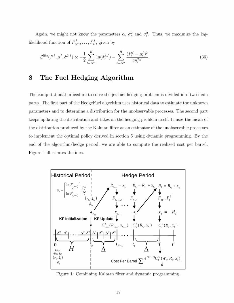
8 The Fuel Hedging Algorithm

The computational procedure to solve the jet fuel hedging problem is divided into two main

parts. The first part of the HedgeFuel algorithm uses historical data to estimate the unknown

parameters and to determine a distribution for the unobservable processes. The second part

keeps updating the distribution and takes on the hedging problem itself. It uses the mean of

the distribution produced by the Kalman filter as an estimator of the unobservable processes

to implement the optimal policy derived in section 5 using dynamic programming. By the

end of the algorithm/hedge period, we are able to compute the realized cost per barrel.

Figure 1 illustrates the idea.

Historical Period

KF Initialization

trΔ trΔL0 NtH

trΔ trΔ trΔ trΔ

1−NtΔ

LT1t 't

1−Ntx

1tx

KF Update

Hedge Period

Δ( )00 ,ξχ

Prior dist. for

0β

ot

ft

ttt

ttt

t PP

F

Fy

n

,ln

ln

'

'1

,

,

⎥⎥⎥

⎦

⎤

⎢⎢⎢

⎣

⎡=

+

+

M

),(111

fl−−− NNN ttt xRC ),(

111

flttt xRC

TT Rx −=

221 ttt xRR +=

Ntx

NN tt xR =−1

f' , TTt PF

L',1 tt N

F− ',1 ttF

∑−

t

tttl

ttTr

dxRWCe ),,(f)(

Cost Per Barrel

),(flTTT xRC

11 ttT xRR +=

( )NN tt ξχ ,

Ntβ

trΔ trΔ

Figure 1: Combining Kalman filter and dynamic programming.

17

Figure 2 below describes the first part of the jet fuel hedging algorithm, the historical

period. No hedging decision is taken in this part. First, the algorithm requires as input data

both the Kalman filter parameters and an initial normal distribution for the processes, see

steps 1.0 and 1.1. Then, a set of historical future prices are observed, as in step 1.2. After

that, the log-likelihood function (31) is maximized to estimate θ, see step 1.3. Note that

as σχ, σξ and Σν represent standard deviations, we require that they be strictly positive.

Moreover, as ρχξ represents a correlation, it is restricted to be between −1 and 1. Historical

fuel and oil spot prices are observed in steps 1.4, while another maximization procedure takes

place in step 1.5 to estimate the parameters related to the correlation between the oil and

fuel spot prices. As before, the variables representing standard deviations are constrained to

be positive. Finally, the algorithm loops over the historical data and use the Kalman filter

equations to return an updated distribution for the processes.

STEP 1.0: Set the Kalman filter parameters: ∆tr, H and T ′.

STEP 1.1: Set the prior distribution for (χ0, ξ0) and β0.

STEP 1.2: Observe y∆tr , . . . , yH∆tr .

STEP 1.3: Determine θ = (κ, σχ, σξ, ρχξ, λχ, µ∗ξ , µξ) maximizing Llike(y, µy, Σy) (see (31))

subject to σχ > 0, σξ > 0, −1 ≤ ρχξ ≤ 1, Σν ≥ 0.

STEP 1.4: Observe P o∆tr , . . . , P o

H∆tr and P f∆tr , . . . , P

fH∆tr .

STEP 1.5: Determine (α, ση, σε) maximizing Llike(P f , µf , σ̂2,f ) (see (36))

subject to ση > 0, σε > 0.

STEP 1.6: Do for t = ∆tr, 2∆tr, . . . , H∆tr:

STEP 1.6.a: Update the distribution of (χt, ξt) using (27)-(30)

STEP 1.6.b: Update the distribution of βt using (33)-(35)

Figure 2: FuelHedge Algorithm Part 1 - Historical Period

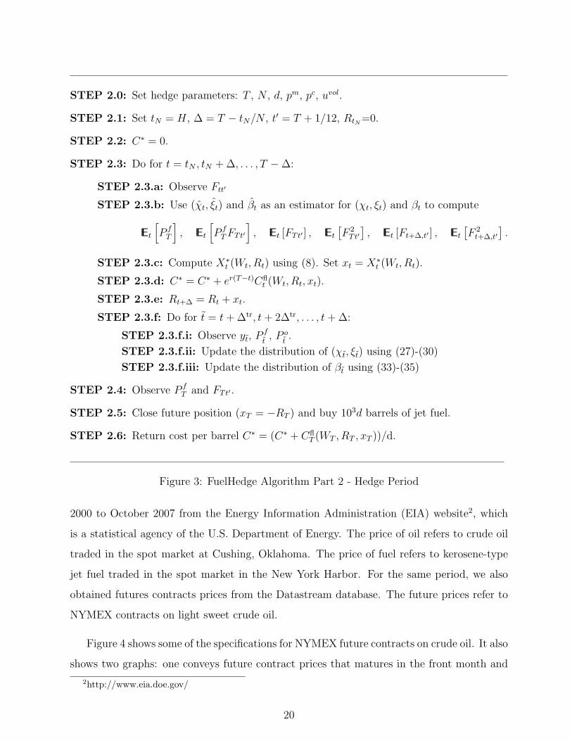
Figure 3 describes the second part of the algorithm, the hedge period. It uses the distri-

bution obtained in the first part as its initial distribution. First, the algorithm requires as

18

an input the hedge parameters, see step 2.0. It assumes the beginning of the hedge period

coincides with the end of the historical period, as tN = H. Nevertheless, the hedge period

can start any time after the historical one. However, the longer the interval, the less accurate

the distribution, since it was last updated using prices in the past. Given our assumption

that the trade dates are equally spaced, step 2.1 also computes the interval ∆ between them.

We have also assumed that the maturity date of the future contracts is one month after the

hedging period and that the initial future position is equal to zero. Step 2.2 initializes the

cost per barrel following our policy.

At each trading date, the algorithm observes the current price of the future contract

maturing at t′, see step 2.3.a. Using this information and the current mean of the unobserv-

able processes as an estimator, it computes both the expected values required to determine

the trading decision and the trading decision itself, see steps 2.3.b and 2.3.c. The decision

generates a cashflow, given by (4), that is used to update the cost per barrel, see step 2.3.d.

The decision also affects the number of future contracts standing, see step 2.3.e.

In between two trading dates, the algorithm keeps observing future/spots prices and

using the Kalman filter equations to update the distribution of the unobservable processes,

see steps 2.3.f.i-2.3.f.iii.

Finally, at the end of the hedge period, the algorithm observes the current future and

fuel spot prices, see step 2.4. Then, the future position is closed and jet fuel is bought to

meet the demand, see step 2.5. The algorithm terminates returning the realized cost per

barrel.

9 Numerical Experiments

We compare our strategy to the hedging strategies described in section 4, since these are the

ones widely used in practice. We use actual price data to run the experiments.

We start by describing the data. We obtained weekly oil and fuel spot prices from January

19

STEP 2.0: Set hedge parameters: T , N , d, pm, pc, uvol.

STEP 2.1: Set tN = H, ∆ = T − tN/N , t′ = T + 1/12, RtN =0.

STEP 2.2: C∗ = 0.

STEP 2.3: Do for t = tN , tN + ∆, . . . , T −∆:

STEP 2.3.a: Observe Ftt′

STEP 2.3.b: Use (χ̂t, ξ̂t) and β̂t as an estimator for (χt, ξt) and βt to compute

IEt

[P f

T

], IEt

[P f

T FTt′

], IEt [FTt′ ] , IEt

[F 2

Tt′

], IEt [Ft+∆,t′ ] , IEt

[F 2

t+∆,t′

].

STEP 2.3.c: Compute X∗t (Wt, Rt) using (8). Set xt = X∗

t (Wt, Rt).

STEP 2.3.d: C∗ = C∗ + er(T−t)Cflt (Wt, Rt, xt).

STEP 2.3.e: Rt+∆ = Rt + xt.

STEP 2.3.f: Do for t̃ = t + ∆tr, t + 2∆tr, . . . , t + ∆:

STEP 2.3.f.i: Observe yt̃, P f

t̃, P o

t̃.

STEP 2.3.f.ii: Update the distribution of (χt̃, ξt̃) using (27)-(30)

STEP 2.3.f.iii: Update the distribution of βt̃ using (33)-(35)

STEP 2.4: Observe P fT and FTt′ .

STEP 2.5: Close future position (xT = −RT ) and buy 103d barrels of jet fuel.

STEP 2.6: Return cost per barrel C∗ = (C∗ + CflT (WT , RT , xT ))/d.

Figure 3: FuelHedge Algorithm Part 2 - Hedge Period

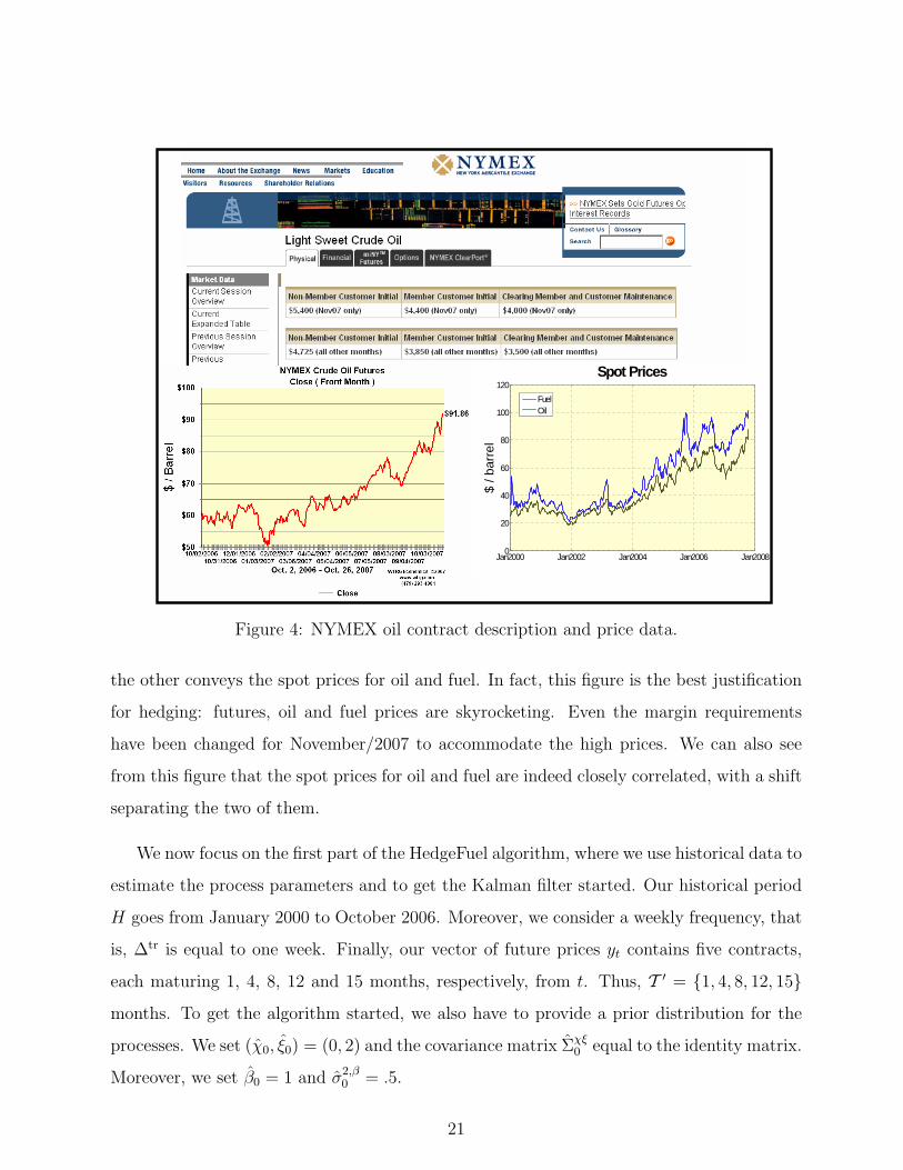
2000 to October 2007 from the Energy Information Administration (EIA) website2, which

is a statistical agency of the U.S. Department of Energy. The price of oil refers to crude oil

traded in the spot market at Cushing, Oklahoma. The price of fuel refers to kerosene-type

jet fuel traded in the spot market in the New York Harbor. For the same period, we also

obtained futures contracts prices from the Datastream database. The future prices refer to

NYMEX contracts on light sweet crude oil.

Figure 4 shows some of the specifications for NYMEX future contracts on crude oil. It also

shows two graphs: one conveys future contract prices that matures in the front month and

2http://www.eia.doe.gov/

20

Jan2000 Jan2002 Jan2004 Jan2006 Jan20080

20

40

60

80

100

120

$ / b

arre

l

Spot Prices

FuelOil

Figure 4: NYMEX oil contract description and price data.

the other conveys the spot prices for oil and fuel. In fact, this figure is the best justification

for hedging: futures, oil and fuel prices are skyrocketing. Even the margin requirements

have been changed for November/2007 to accommodate the high prices. We can also see

from this figure that the spot prices for oil and fuel are indeed closely correlated, with a shift

separating the two of them.

We now focus on the first part of the HedgeFuel algorithm, where we use historical data to

estimate the process parameters and to get the Kalman filter started. Our historical period

H goes from January 2000 to October 2006. Moreover, we consider a weekly frequency, that

is, ∆tr is equal to one week. Finally, our vector of future prices yt contains five contracts,

each maturing 1, 4, 8, 12 and 15 months, respectively, from t. Thus, T ′ = {1, 4, 8, 12, 15}

months. To get the algorithm started, we also have to provide a prior distribution for the

processes. We set (χ̂0, ξ̂0) = (0, 2) and the covariance matrix Σ̂χξ0 equal to the identity matrix.

Moreover, we set β̂0 = 1 and σ̂2,β0 = .5.

21

Table 1 shows the estimated values for the parameters. The log likelihood functions were

maximized using the Matlab function fminunc. Figure 5 shows both the actual oil spot

prices and the estimated one, using the Kalman filter. We can infer that the two-factor price

model did reflect the actual price behavior and the Kalman filter did do a good job tracking

the two unobservable processes.

Processes (χt, ξt) parameters Process βt parametersκ 1.7501 σξ 0.1813 α 8.1025

ρχξ 0.4032 σ2ν1

0.0285 σ2ε 0.0001

λχ 0.2439 σ2ν2

0.0062 σ2η 0.1286

µ∗ξ 0.0120 σ2ν3

0.0100µξ 0.0744 σ2

ν40.0000

σχ 0.6429 σ2ν5

0.0125

Table 1: Estimated parameters using actual prices from Jan/2000 to Oct/2006

Figure 5: Kalman filter - Observed and estimated oil spot price

We close this part by reporting the updated processes distributions. We obtained

(χ̂H , ξ̂H) =

[−0.13424.2542

]and Σ̂χξ

H = 10−3

[0.2025 −0.0351−0.0351 0.0061

].

22

Moreover, β̂H = 1.1286 and σ̂2,βH = 5.5039−11. We note that the standard deviations are

pretty small, indicating that the estimators (the mean distribution) should be quite reliable.

In all the experiments, we consider the hedge period to be one year, i.e., T = 1 year.

We also consider four trading opportunities, implying that the time between two consecutive

decision dates is three months. Thus, N = 4 and ∆ = 3 months. We have set the interest

rate to zero and the demand to be 100 contracts. We note that picking the day/time to

execute the trading order is out of the scope of this work.

First, we want to see how our strategy compares to the other strategies. We consider

the price data from January/2000 to the end of October/2006 as our historical period. The

hedge period goes from November/2006 to November/2007. It is a simulation exercise, as we

want to consider several runs in order to observe the sample volatility of the price per barrel

under the different approaches. Thus, we have used the price models introduced in section 6

(considering the parameter values described in table 1) to simulate 300 different sets of weekly

prices over the hedging period. Of course, our algorithm still assumed the processes were

unobservable and the Kalman filter equations were used to produce the processes estimators.

We used the same estimators for the competing policies.

Figure 6 shows the price per barrel produced by the different hedging strategies, when

the volatility weight for our approach ranged from .2 to .5. It also shows the 95% upper

confidence bound for the prices. Comparing the price produced by the No-Hedge strategy

with the actual fuel price for November/2007 conveyed in figure 4, we can see that the

simulation produced a realistic outcome. We can also observe that the higher the volatility

weight, the smaller the sample volatility. Clearly, the reduction in volatility resulted in

a higher mean cost per barrel. Small weight values indicates the investor is emphasizing

speculation rather than hedging.

Note that the graph is divided into seven regions. Region I corresponds to very small

volatility weights. We can observe the gambling nature of our approach: very low mean

price per barrel but substantial risk. In region II, even though the weights are still small

and the risks are still large, our approach does better than not hedging at all. In region III,

we dominate the hedge-and-forget OHR strategy, providing smaller costs and smaller risks.

23

95% confidence upper bound

I II III IV V VI VII

No

Hed

geOur

s

OH

R

OH

Rt

Nai

ve

Figure 6: Simulated price per barrel - Projection to Nov/2007

On the other hand, there is no clear dominance between our approach and the dynamic

OHR approach over regions IV and VI. The investor has to decide what suits his needs

best: either a better price per barrel or a smaller risk. Region V shows a narrow range for

which the dynamic OHR dominates our approach by small margins. Finally, in region VII

we outperform the naive approach.

We can infer from this experiment that considering a more elaborate utility function

does pay off. More importantly, the ability to turn a knob on the volatility weight allows

the investor to decide which level of price/risk he is more comfortable with.

Figure 7 illustrates the speculative nature of our policy for different weights (using the

same sample path). Each figure shows the decision (buying or selling), the number of con-

tracts outstanding, and the final demand, over the horizon.

The strategy follows the same pattern for all the different weights; the difference is the

24

2.=volu 3.=volu

4.=volu 5.=volu

Figure 7: Trading decisions and number of contracts standing for the November 2006-2007hedging period

size of the future position. Since in the current market situation the oil/fuel prices are

trending upward, the strategy tells the investor to buy several contracts, more than the

actual demand, in the beginning of the hedge period. Then, as the prices reveal themselves

along time, the strategy is to rebalance the position selling some of the contracts. Note that

the higher the volatility weight, the closer to the actual demand is the number of contracts

standing by the end of the period. The high speculative nature of the strategy can be

observed when uvol = .2, as the number of contracts standing is way beyond the demand.

We conclude this section showing the actual price per barrel if we were to follow the

different approaches on a weekly basis. As before, the hedging period is one year and there

are four trading opportunities. Figure 8 conveys the actual prices for volatility weights equal

to .2, .3, .4 and .5. The reported price for a given month/year assumes that the hedging

25

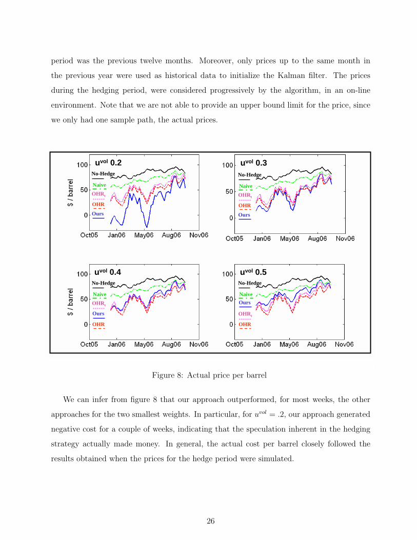
period was the previous twelve months. Moreover, only prices up to the same month in

the previous year were used as historical data to initialize the Kalman filter. The prices

during the hedging period, were considered progressively by the algorithm, in an on-line

environment. Note that we are not able to provide an upper bound limit for the price, since

we only had one sample path, the actual prices.

No-Hedge

uvol 0.2 uvol 0.3

uvol 0.5uvol 0.4

Ours

OHRt

OHR

Naive

No-Hedge

Ours

OHRt

OHR

Naive

No-Hedge

Ours

OHRt

OHR

Naive

No-Hedge

Ours

OHRt

OHR

Naive

Figure 8: Actual price per barrel

We can infer from figure 8 that our approach outperformed, for most weeks, the other

approaches for the two smallest weights. In particular, for uvol = .2, our approach generated

negative cost for a couple of weeks, indicating that the speculation inherent in the hedging

strategy actually made money. In general, the actual cost per barrel closely followed the

results obtained when the prices for the hedge period were simulated.

26

10 Conclusions and Further Research

We proposed a novel trading strategy for the jet fuel hedging problem using oil future

contracts. Our policy is optimal with respect to a utility function that considers risk, return

and a prospective test on the hedge effectiveness. Moreover, different levels of risk aversion

are taken into consideration through a parameter set by the investor. On the contrary, the

most traditional strategy is the one that only minimizes the risk.

We gathered actual price data and compared our strategy to other well established ap-

proaches. We were able to observe that it dominates the others for certain risk levels. In

addition to that, the algorithmic procedure to compute our policy, combining dynamic pro-

gramming and Kalman filter, is very practical and easy to implement. We can thus conclude

that our approach can be quite useful for practitioners.

We also analyzed the nature of our policy. As expected, if the tolerance for risk is high,

it has a speculative nature. On the other hand, the more risk averse, the more the policy

concentrates only on hedging, generating higher but more stable costs per barrel.

A future direction for research is the consideration of transaction costs in the utility func-

tion, as trading future contracts usually involves brokerage commissions and margin require-

ments. However, when these costs are incorporated in our utility function, the corresponding

dynamic program can not be solved analytically, leading to the curse of dimensionality. It

would be necessary to consider a technique such as approximate dynamic programming to

produce a trading policy that reflects such costs.

References

Baillie, R. T. & Myers, R. J. (1991), ‘Bivariate estimation of the optimal commodity futures

hedge’, Journal of Applied Econometrics 6(1), 109–124. 4

Bertsimas, D., Kogan, L. & Lo, A. W. (2001), ‘Hedging derivative securities and incomplete

markets: An e-arbitrage approach’, Operations Research 49(3), 372 – 397. 5

27

Bollerslev, T. (1986), ‘Generalized autoregressive conditional heteroskedasticity’, Journal of

Econometrics 31(3), 307–327. 4

Bos, C. & Gould, P. (2007), Dynamic correlations and optimal hedge ratios. Discussion

paper. Department of Econometrics & O.R., Vrije Universiteit Amsterdam. 3, 4, 11

Carter, D., Rogers, D. & Simkins, B. (2006), ‘Does hedging affect firm value? evidence from

the us airline industry’, Financial Management 35(1), 53–86. 1

Cecchetti, S., Cumby, R. & Figlewski, S. (1988), ‘Estimation of the optimal futures hedge’,

Review of Economics and Statistics 70(4), 623–630. 4, 5

Chen, S. S., Lee, C. F. & Shrestha, K. (2003), ‘Futures hedge ratios: a review’, The Quarterly

Review of Economics and Finance 43(1), 433–465. 4

Duffie, D. (1992), Dynamic Asset Pricing Theory, Princeton University Press. 12

Engle, R. F. (1982), ‘Autoregressive conditional heteroscedasticity with estimates of the

variance of united kingdom inflations’, Econometrica 50(1), 987–1008. 4

Haigh, M. S. & Holt, M. T. (2002), ‘Combining time-varying and dynamic multi-period

optimal hedging models’, European Review of Agriculture Economics 29(4), 471–500. 4

Harvey, A. C., Ruiz, E. & Shephard, N. (1994), ‘Multivariate stochastic variance models’,

Review of Economic Studies 61(2), 247–264. 4

Heath, D., Platen, E. & Schweizer, M. (2001), ‘A comparison of two quadratic approaches

to hedging in incomplete markets’, Mathematical Finance 11(4), 385413. 5

Hull, J. (2000), Options, Futures, and Other Derivatives, Prentice Hall. 4

Hung, J. C., Chiu, C. L. & Lee, M. C. (2005), ‘Hedging with zero-value at risk hedge ratio’,

Applied Financial Economics 16(1), 259269. 5

Jacquier, E., Polson, N. G. & Rossi, P. E. (1994), ‘Bayesian analysis of stochastic volatility

models (with discussion)’, Journal of Business and Economic Statistics 12(4), 371–417. 4

28

Laurent, J. P. & Pham, H. (1999), ‘Dynamic programming and mean-variance hedging’,

Journal Finance and Stochastics 3(1), 83–110. 5

Lee, M. C. & Hung, J. C. (2007), ‘Hedging for multi-period downside risk in the presence of

jump dynamics and conditional heteroskedasticity’, Applied Economics 1(1), 1–10. 5

Lien, D. H. D. & Tse, Y. K. (2002), ‘Some recent developments in futures hedging’, Journal

of Economic Surveys 16(1), 357–383. 2, 4

Morrell, P. & Swan, W. (2006), ‘Airline jet fuel hedging: Theory and practice’, Transport

Reviews 26(6), 713–730. 1

Schwartz, E. & Smith, J. (2000), ‘Short-term variations and long-term dymanics in com-

modity prices’, Management Science 46(7), 893–911. 3, 10

Tunaru, R. & Tan, M. (2002), Minimizing risk techniques for hedging jet fuel: an economet-

rics investigation. Discussion paper. Bussiness School, Middlesex University. 4

Zea, M. (2004), Is airline industry risk unmanageable?, Technical report, Mercer on Travel

and Transport. 1

29