Industrial & Labor Relations ReviewVolume 64Number 4 JULY 2011 Article 5

2011

Does a Higher Minimum Wage Enhance theEffectiveness of the Earned Income Tax Credit?David NeumarkUniversity of California, Irvine, dneumark@uci.edu

William WascherFederal Reserve Board, william.l.wascher@frb.gov

Neumark, David and Wascher, William (2011) "Does a Higher Minimum Wage Enhance theEffectiveness of the Earned Income Tax Credit?," Industrial & Labor Relations Review, Vol. 64, No. 4,article 5.Available at: http://digitalcommons.ilr.cornell.edu/ilrreview/vol64/iss4/5

Does a Higher Minimum Wage Enhance the Effectiveness of the EarnedIncome Tax Credit?

The authors estimate the effects of the interactions between the Earned Income Tax Credit (EITC) andminimum wages on labor market outcomes. They use information on policy variation from the Departmentof Labor’s Monthly Labor Review, reports published by the Center on Budget and Policy Priorities, and dataon individuals and families from the Current Population Survey to assess the economic impact of minimumwages and the EITC on families. Their results indicate that for single women with children, the EITC boostsemployment and earnings, and coupling the EITC with a higher minimum wage enhances this positive effect.Conversely, for less-skilled minority men and for women without children, employment and earnings aremore adversely affected by the EITC when the minimum wage is higher. Turning from individuals to families,for very poor families with children a higher minimum wage appears to enhance the effects of the EITC.Whether the policy combination of a high EITC and a high minimum wage is viewed as favorable orunfavorable depends in part on whom policymakers are trying to help.

Earned income tax credit, minimum wage

This article is available in Industrial & Labor Relations Review: http://digitalcommons.ilr.cornell.edu/ilrreview/vol64/iss4/5

712

Industrial and Labor Relations Review, Vol. 64, No. 4 (July 2011). © by Cornell university.0019-7939/00/6404 $05.00

DoeS A HIGHer mINImum WAGe

eNHANCe THe eFFeCTIVeNeSS oF

THe eArNeD INCome TAX CreDIT?

DAVID NeumArK AND WIllIAm WASCHer*

The authors estimate the effects of the interactions between the earned In-come Tax Credit (eITC) and minimum wages on labor market outcomes. They use information on policy variation from the Department of labor’s Monthly Labor Review, reports published by the Center on budget and Policy Priorities, and data on individuals and families from the Current Population Survey to assess the economic impact of minimum wages and the eITC on families. Their results indicate that for single women with children, the eITC boosts employment and earnings, and coupling the eITC with a higher mini-mum wage enhances this positive effect. Conversely, for less-skilled minority men and for women without children, employment and earnings are more adversely affected by the eITC when the minimum wage is higher. Turning from individuals to families, for very poor families with children a higher minimum wage increases the positive impact of the eITC on incomes, so that a higher minimum wage appears to enhance the effects of the eITC. Whether the policy combination of a high eITC and a high minimum wage is viewed as favorable or unfavorable depends in part on whom policymakers are trying to help.

* David Neumark is Professor of economics at the uni-versity of California, Irvine, a research Associate of the National bureau of economic research, and a research Fellow of IZA. William Wascher is Senior Associate Di-rector in the Division of research and Statistics at the Federal reserve board. The authors are grateful to Stephen Ciccarella and elizabeth elzer for outstanding research assistance and to Paul bingley, marianne bitler, Nada eissa, martin Feldstein, roger Gordon, Hilary Hoynes, and Jim Poterba for helpful comments. A preliminary

introduced their own eITC programs, which typically provide families in the state with a percentage supplement to the federal eITC. The number of states with such an eITC increased from seven states in 1996 to 19 states and the District of Columbia in 2007, boosting the percentage of the 16- to 64-year-old population residing in states

enacted in 1975, the earned Income Tax Credit (eITC) has become a staple of

u.S. antipoverty policy. During the 1980s and 1990s, the eITC was expanded at the federal level, with the credit rate rate rising from 10% in 1984 to 40% (for families with two children) in 1996, where it has re-mained since. moreover, some states have

version of this paper was presented at the Trans- Atlantic Public economics Seminar on Income Taxa-tion, June 12–13, 2008. Neumark received some support for the early stages of research on this project from the employment Policies Institute. The views expressed in this paper do not necessarily reflect the views of the Federal reserve board or the employment Policies Institute. The data and programs used in this paper will be available upon request by writing to dneumark@uci .edu for three years after the date of publication.

THe mINImum WAGe AND THe eArNeD INCome TAX CreDIT 713

supplementing the federal eITC from 14% to nearly 40%.1

Previous studies of the eITC have typi-cally shown that this program is effective at increasing the labor force attachment and earnings of low-income women and families with children. For example, eissa and liebman (1996) demonstrated that the fed-eral eITC increases employment of young, unskilled women with children; meyer (2002) concluded that a higher federal or state credit boosts employment of single mothers; Grogger (2003) reported positive effects of the federal eITC on employment and earnings of female-headed families; and liebman (1998) and Scholz (1994) found that a large proportion of eITC payments go to poor families.2 likewise, our own previous research has indicated that the eITC outper-forms the minimum wage in terms of its beneficial effects on the distribution of fam-ily earnings.3

Some researchers have pointed out, how-ever, that the labor supply response associ-ated with the eITC may cause the market wage to fall.4 If so, some of the gains from

1 This calculation is based on the CPS data described below. The 19 states with eITC supplements in 2007 were Delaware, Illinois, Indiana, Iowa, Kansas, maine, maryland, massachusetts, minnesota, Nebraska, New Jersey, New mexico, New York, oklahoma, oregon, rhode Island, Vermont, Virginia, and Wisconsin. The supplemental eITC in those states ranged from 4% to 43% of the federal credit. In addition, eITC supple-ments became effective in 2008 in louisiana, michigan, and North Carolina, and a supplement took effect in Washington State in 2011. 2 See Hoffman and Seidman (2003) and Hotz and Scholz (2003) for extensive surveys of previous research on the eITC. leigh (2010) also found evidence of a positive supply response on the intensive margin (hours). The only study we know of that fails to find positive labor supply effects on those likely to be eligible for the eITC is Cancian and levinson (2005), which ex-amined the effects of Wisconsin’s higher eITC supple-ment for families with three children.3 Indeed, the minimum wage appears to have no benefi-cial effects on low-income families and may even ad-versely affect them. See Neumark and Wascher (2001), as well as burkhauser et al. (1996) and Neumark and Wascher (2008).4 See, for example, leigh (2010) and rothstein (2008), who found that an increase in the generosity of the eITC puts downward pressure on the wages of low-skilled workers already in the labor market.

the eITC that are intended for eligible work-ers will instead be reaped by employers, and there may be negative spillovers on the wages and incomes of low-skilled workers not eligible for the eITC.5 In light of these po-tential general equilibrium effects, some economists and policymakers have pointed to the minimum wage as a way to mitigate any fall in wages. In particular, these advo-cates claim that the eITC and the minimum wage may be mutually reinforcing—that is, complementary—with a higher minimum wage enhancing the effectiveness of the eITC in helping poor and low-income families.6

In this paper, we examine potential inter-actions between the eITC and the minimum wage. At a theoretical level, some models suggest that the two policies reinforce each other, whereas others propose that they off-set each other, at least for some subgroups of the population. In our view, the most com-pelling theoretical perspective allows for heterogeneity of individuals who would earn wages near the minimum if they worked. In that case, either a minimum wage or an eITC can induce some individuals to enter the labor market, perhaps (especially in the case of the minimum wage) displacing others of lower productivity.7 There may be other indi-

5 As explained below, a very small eITC payment is avail-able to families without children. As a result, many low-skilled workers (unless they are under age 25 or over age 64) are not strictly “ineligible” for the eITC but rather are simply unlikely to gain much from it. We use “ineligible” as a short-hand term when we refer to ob-servations on those who are not eligible for the much more generous eITC available to families with children. Similarly, when we refer to the “childless” or those “without children,” we mean those who do not have children in the home. This is what the CPS measures as well as what determines eligibility for the eITC (which is based on whether the child lived with a person more than six months during the tax year). 6 See, e.g., bernstein (2004); Fiscal Policy Institute (2004); and levitis and Johnson (2006).7 The conventional theory does not imply that employ-ment of any particular subgroup will decrease in re-sponse to a higher minimum wage; it only predicts that overall labor demand for less-skilled workers will fall. In particular, individuals for whom the market wage was previously below the reservation wage could, after a minimum wage increase, be drawn into the labor force. For example, Neumark and Wascher (1996) found that an increase in the minimum wage induces some

INDuSTrIAl AND lAbor relATIoNS reVIeW714

viduals with higher reservation wages, how-ever, who enter the labor market only when there is both a high minimum wage and a more generous eITC. If these individuals are the ones to whom the government would like to try to redistribute income (e.g., if sin-gle mothers with children have particularly high reservation wages among roughly com-parably skilled workers), then combining the eITC with a higher minimum wage may enhance the beneficial distributional effects of the eITC.

Conversely, for groups less likely to be eli-gible for the eITC, such as teenagers and low-skilled adult males, a high minimum wage coupled with an eITC could represent a “double hit,” with the minimum wage re-ducing their employment prospects via the higher wage floor imposed on employers and the eITC reducing their employment prospects via the increased supply of women entering the labor market. Thus, the effects of interactions between these policies, and how these interactive effects vary across dif-ferent groups, are potentially quite complex. Widespread interest in the effectiveness of these policies at the federal level, along with the increasing number of states implement-ing state eITCs as well as higher state mini-mum wages, makes it important to study how they interact.

Minimum Wage-eItc Interactions

The limited research that compares the effects of minimum wages and the eITC has generally not considered the potential for interactions between the two policies.8

higher-skilled teenagers to leave school and enter the labor market.8 one exception is leigh (2010, p. 25, footnote 20) who noted in a footnote that he included an interaction be-tween the minimum wage and the eITC in one of his regressions that examined the effects of the eITC on low-skilled wages. His specification is broadly similar to ours, in that he identified eITC effects from the varia-tion in state eITC supplements. However, we explore much more fully the effects of interactions between the minimum wage and the eITC on the labor market out-comes of individuals and families both eligible and in-eligible for the eITC; his specification was simply reported as a robustness check of his finding that a higher eITC lowers wages for unskilled workers.

However, the policies are not mutually ex-clusive, and, in practice, many individuals are subject to both, raising the possibility that such interactions could arise. Indeed, several arguments regarding how a higher minimum wage could enhance the effective-ness of the eITC have been put forward. Al-though some are clearly invalid, others are possible but require empirical testing to which they have not heretofore been subjected.

one argument often made by minimum wage advocates is that a higher minimum wage is necessary to prevent or mitigate the reduction in market wages associated with the labor supply response to a more gener-ous eITC. In the simplest model of the labor market—a competitive labor market with homogeneous labor—it is clearly wrong to argue that a higher minimum wage will en-hance the effectiveness of the eITC. In this setting, the eITC induces a labor supply in-crease among eligible individuals that, in the absence of a minimum wage, would be ex-pected to result in a lower wage and higher employment for low-wage workers. A mini-mum wage will reduce the extent to which the wage can fall in response to the increase in labor supply, but this will, in turn, reduce the job opportunities available to individuals who enter the labor market because of the eITC. In the extreme case in which all eITC-eligible individuals are priced out of the labor market by the minimum wage, the eITC would result not in any change in em-ployment, but rather in an increase in unem-ployment. In a less extreme case, the eITC induces those with children to enter the labor market, and the burden of excess labor supply is shared between eITC eligibles and ineligibles. In this case, it might appear that the combined policies have distributional benefits from shifting employment towards those eligible for the eITC. However, even more of the eITC-eligibles would be em-ployed in the absence of the minimum wage.

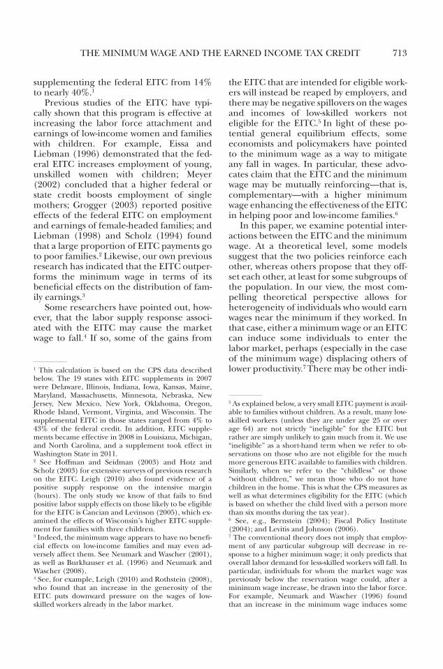
This intuition is illustrated in Figure 1. In the absence of a minimum wage or an eITC, the equilibrium levels of employment (e0) and the market wage (W0) are determined by the intersection of the labor demand

THe mINImum WAGe AND THe eArNeD INCome TAX CreDIT 715

curve (lD) and the labor supply curve (lS). If an eITC is implemented, which we over-simplify by modeling it as a simple tax credit,9 then the labor supply curve shifts out to ls', with equilibrium employment level e1 (and a lower market wage W1). If a minimum wage of Wmin is introduced as well, the wage does not fall as far, but the minimum wage re-duces employment, generating excess labor supply. Indeed, if the minimum wage is set at W0, the eITC has no effect on the labor mar-ket, except to increase the excess of labor supply over the quantity of labor demanded. more generally, in the model with homoge-nous labor, the minimum wage inevitably leads to lower employment and a higher wage than would be the case with the eITC; the eITC simply determines the wage and employment level that would otherwise pre-vail. Any claims about the effectiveness of the minimum wage boil down to the usual

9 The discussion ignores variation in the size of the credit with family income and family structure. The qualitative effect of increasing labor supply is, however, captured in the figure.

debate and are not related to interactions between the two policies.

This analysis also undermines the argu-ment that the minimum wage needs to keep up with inflation (whether by formal index-ation or by more frequent increases) to maintain the effectiveness of the eITC. Pro-ponents of the minimum wage note that be-cause the maximum credit that a family can receive is indexed to inflation whereas the minimum wage is not, a family that receives the eITC and for which earnings partly de-pend on minimum wage work will tend to face a declining real eITC payment when the real value of minimum wage declines.10

This argument ultimately rests on the idea that a higher minimum wage—regardless of the generosity of the eITC—will help low-income families; thus, it is really an argu-ment about the distributional effects of the minimum wage rather than an argument that a higher minimum wage increases the effectiveness of the eITC. In this regard, the research literature fails to find positive

10 See economic Policy Institute (2004).

LS′

Figure 1. minimum Wages and the eITC in a Competitive labor market

INDuSTrIAl AND lAbor relATIoNS reVIeW716

distributional effects of the minimum wage,11 suggesting that poor and low-income fami-lies would be no better off on average with an eITC coupled with a higher minimum wage than with an eITC alone.

Different arguments are therefore neces-sary in order to make the case that a higher minimum wage complements the eITC. one of these is to drop the assumption of a com-petitive labor market. For example, some re-searchers have claimed that low-skilled labor markets are better characterized by monop-sony power stemming from labor market frictions.12 In such a case, a minimum wage could increase employment and earnings of less-skilled workers, making more of them eligible for eITC payments or raising the size of the payments for which they are eli-gible. our recent exhaustive review of the effects of minimum wages on employment concludes, however, that the body of evi-dence is much more consistent with the com-petitive model of labor markets (Neumark and Wascher 2007a).

An alternative argument holds that a higher minimum wage may reduce the dis-tortionary impact of the eITC on labor sup-ply. In particular, a higher minimum wage enables a family to achieve the same level of income (earnings plus eITC) at the maxi-mum eITC credit with a smaller eITC pay-ment. This, in turn, results in a lower marginal tax rate over the phase-out range of the credit, which could reduce the associ-ated labor supply disincentives (blank and Schmidt 2001). This argument, though, is really about the eITC parameters rather than the minimum wage. That is, it does not imply that, for a given set of eITC parame-ters, a minimum wage makes the eITC more effective in reducing poverty or helping low-income families. rather, it suggests that with a higher minimum wage we might observe a different set of eITC parameters that have better distributional effects than the eITC parameters chosen when the minimum wage is lower. because this hypothesis is not

11 For a review of the evidence, see Neumark and Wascher (2008).12 See, for example, manning (2003) and machin and manning (1994).

explicitly about minimum wage-eITC inter-actions, testing it is beyond the scope of this paper.

A more promising avenue for motivating interactions between minimum wages and the eITC in terms of their effects on low- income families is to allow for heterogeneity of individuals who would earn wages near the minimum if they worked. Suppose that there are two types of workers: (a) teenagers in middle-income families (ineligible for the eITC) with a low reservation wage; and (b) poor single mothers who are eligible for the eITC, are slightly more productive than teenagers, and have significantly higher res-ervation wages, perhaps because of fixed costs of working (e.g., paying for child care). In the absence of a minimum wage and with no eITC, the difference in reservation wages can lead to a situation in which the teenag-ers are employed while the single mothers are not.

Suppose just the minimum wage is raised. For a sufficiently high minimum, some teen-agers will become non-employed. Demand will shift towards more-skilled single moth-ers, but the market wage (or the higher min-imum) may still fall short of their reservation wage. In this case, the minimum wage deliv-ers no benefit to poor single mothers be-cause they are not drawn into the labor market. If just the eITC is raised (in particu-lar, the phase-in rate), the effective wage may still fall short of the reservation wage, in which case teenagers will continue to be em-ployed (since their wage has not changed), but again, poor single mothers are no better off. A higher eITC coupled with a higher min-imum wage, however, may raise the effective wage above the reservation wage of single mothers, leading to more substitution of single mothers for teenagers, and hence bet-ter distributional effects of the eITC. Ac-cording to this argument, the distributional effect of the eITC is enhanced by a higher minimum wage, which gives rise to an inter-active effect.13

13 If mothers are no more productive than teenagers, then although more mothers may be drawn into the labor market, employers are indifferent between the two groups and so demand does not shift toward them.

THe mINImum WAGe AND THe eArNeD INCome TAX CreDIT 717

eITC in isolation (taking us back to a case similar to that depicted in Figure 1).

In addition, low-skilled individuals who are not eligible for the eITC can take a dou-ble hit from a high minimum wage coupled with an eITC. The minimum wage would re-duce their employment prospects via the higher wage imposed on employers, and the eITC would reduce their employment pros-pects via the increased labor supply of eITC-eligible individuals. For example, in the model described above, the minimum wage plus eITC combination leads to more labor market entry by the higher-skilled workers—single mothers—and hence more disemploy-ment of the lower-skilled workers—teenagers, in that example—but more generally low-skilled individuals without children living in the home.

The period 1997–2007 is a propitious time in which to study the effects of policy interactions between the minimum wage and the eITC. Paralleling the rapid prolifer-ation of state eITCs was a similar expansion in state minimum wages, with the number of states with minimum wages above the fed-eral minimum rising to 29 (plus the District of Columbia) as of the beginning of 2007. At the same time, focusing on the post-welfare reform period allows us to abstract from major changes in work incentives associated with the transition from Aid to Families with Dependent Children (AFDC) to Temporary Assistance to Needy Families (TANF). Al-though welfare policies continued to change after TANF was enacted in 1996, preliminary analyses indicated that state-level variation in key welfare reforms (such as time limits and work requirements) that were imple-mented after 1996 did not have discernible effects on the dependent variables we study, and so we focus on minimum wage-eITC interactions.15

15 This is not to say that the change from AFDC to TANF had no effects on labor market outcomes. Grogger (2003) found evidence that the imposition of time lim-its (the timing of which varied across states with TANF implementation) led to employment increases among women with younger children for whom time limits were a more binding constraint. our sample period be-gins in 1997 and thus covers the post-welfare reform period. As a result, the welfare reform effects we can

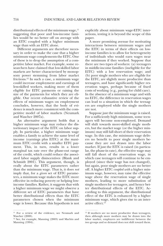
The case for single mothers (assumed here to face a fixed cost of employment) is depicted in Figure 2. The individual’s indif-ference curves between non-working time (t) and earnings (w⋅[T-t]) are given by the curved lines, whereas the budget constraint at the market wage is given by the solid line (with maximum earnings of wT). because of the fixed cost of employment, the individual does not work in the absence of a minimum wage or an eITC. moreover, neither the minimum wage in isolation (which shifts the budget constraint to the dotted and dashed line) nor the eITC in isolation (the dotted line) is sufficient to induce labor market entry. In contrast, the combined policy of both a minimum wage and an eITC (the dashed line) raises the return to work by enough to induce labor market entry. of course, policymakers could devise a set of eITC parameters in isolation that would yield the same interior solution depicted in Figure 2, but fiscal concerns or fears over in-troducing stronger distortions on the phase-out range may place constraints on setting eITC parameters in this way. Indeed, as a consequence of the potential for labor sup-ply disincentives with a very high eITC, it is possible not only that a higher minimum wage could enhance the positive distribu-tional effects of the eITC, but also that the distributional effects of a minimum wage and a modest eITC are better than those of a high eITC that generates the same effec-tive wage along the phase-in range.14

Figure 2 illustrates how a higher mini-mum wage could enhance the effectiveness of the eITC. It is also possible that a higher minimum wage would reduce the effective-ness of the eITC. In particular, if the wages of those eligible for the eITC are already bound by the minimum wage, then a further increase in the wage floor will just reduce their employment relative to the case of an

In this case, the qualitative effect would be the same, but it would be weaker. 14 estimates of the regression models described below can be used to simulate the distributional effects of al-ternative policy combinations and parameters—but such simulations are likely reliable only within the range of the data.

INDuSTrIAl AND lAbor relATIoNS reVIeW718

Data

We combine data on wages, employment, hours, and earnings (individual and family) with state-level information on minimum wages and earned Income Tax Credits for the period 1997–2006. The minimum wage data are compiled from annual summaries of federal and state labor legislation re-ported each year in the Department of la-bor’s Monthly Labor Review.16 most state minimum wages equal or exceed the federal minimum wage, although some states have a minimum wage below the federal level, often applying to small groups of workers not cov-ered by the federal law. because we do not have the detailed information on who is cov-ered by state law and because coverage by the federal minimum wage is extensive, we use the higher of the state or federal mini-mum as the effective state minimum.

The information on state eITCs comes from a series of reports published by the Center on budget and Policy Priorities. State eITCs specify a percentage of the federal eITC that is paid to state taxpayers via the state income tax system, as a “supplement”

identify are mainly the effects of minor timing differ-ences between the states and variation in the state poli-cies adopted. Some of these earlier results are described in Neumark and Wascher (2007b). 16 In the analysis with the annual CPS files, we use the average minimum wage over the year.

to the federal eITC. our state eITC variable is this percentage. In two states, this percent-age varies with the level of income and/or with the number of children. For Wisconsin, where the supplement varies with the num-ber of children, we use the supplement for families with two children (14%). minneso-ta’s eITC is not specified as a simple percent-age of the federal credit, so we use the reported average supplement of 33%.17 Colo-rado formally has an eITC supplement of 10%, but it was suspended beginning in 2002 for lack of funds.18 Although the state credit is refundable in most states, a few states have a nonrefundable (or only partially refund-able) credit and in one state (maryland), the recipient family has a choice; in the latter case, we use the refundable rate on the pre-sumption that most eligible families would prefer that rate. (A refundable eITC gives money back to the family even if there is no tax liability whereas a non-refundable eITC only reduces any existing tax liability.) over the sample period we use, the federal eITC was unchanged with a phase-in tax credit of 40% for families with two or more children, and 34% for families with one child. The federal eITC also provides a very small credit of 7.65% to individuals who have no

17 See http://www.stateeitc.com. 18 See http://www.cbpp.org/cms/?fa=view&id=733.

w

wminT

wT

Fixed cost

tT

Figure 2. minimum Wage–eITC Interactions

THe mINImum WAGe AND THe eArNeD INCome TAX CreDIT 719

children at home and are between the ages of 25 to 64.19

We merge these state-level policy variables with data from CPS Annual Demographic Files (ADF).20 The ADF files are used to con-struct individual-level measures of wages, employment (worked any time last year), and annual hours, as well as demographic and human capital indicators. In addition, we use the ADF files to construct family-level measures of annual earnings and the poverty line for each family. Finally, we append to each record the state unemployment rate in each year to control for variation in eco-nomic conditions at the state-by-year level. The unemployment rate is potentially en-dogenous, but by using the statewide unem-ployment rate (from the local Area unemployment Statistics) rather than a rate for groups more strongly affected by the minimum wage, we hope to capture the ex-ogenous influence of changes in aggregate demand.21

Methods

We use a reduced-form approach to estimate the effects of the interactions be-tween the eITC and minimum wages on labor market outcomes. In principle, one could estimate a structural model of labor

19 In addition to the phase-in rate, the eITC establishes a maximum credit (in 2007, $4,716 for families with two or more children, $2,853 for families with one child, and $428 for individuals with no children at home); a “plateau” or income range over which the maximum benefit remains fixed (in 2007, for families with two or more children, from $11,791–$15,399); and a phase-out rate at which the credit is reduced as income rises fur-ther (currently 21.06% for families with two or more children).20 We also use monthly outgoing rotation group (orG) files for some limited analyses of teenagers. For the analysis of adults using the ADF files, the minimum age cutoff is always 21, to mitigate problems of classifying people based on education (for reasons explained below) when they are still in school.21 We also experimented with the inclusion of state real GDP growth per capita in the various specifications we estimate. However, the estimated coefficient of this vari-able was never statistically significant (in contrast to the estimated coefficient of the unemployment rate), and its inclusion had no impact on the results, so we omit it in the specifications reported in the paper.

supply in the context of a non-linear budget constraint that incorporates changes in both the eITC and the minimum wage (as well as other policy changes).22 However, a reduced-form approach allows us to more naturally extend the prior literature that focused on the effects of the eITC on labor supply and poverty (e.g., Cancian and levinson 2005; eissa and liebman 1996; eissa and Hoynes 2004; Neumark and Wascher 2001) by ex-panding the specifications used in these studies to incorporate interactions between the eITC and the minimum wage. In addi-tion, many potentially eligible individuals have imperfect information about the eITC, and most workers are not able to freely choose their work hours over the course of the year (liebman 1998; romich and Weisner 2000), which may limit the appeal of using an approach based on utility maxi-mization with respect to an explicit non- linear budget constraint.23 Nevertheless, it is clear that the structural and reduced-form approaches are complementary.

We estimate models for individual and family labor market outcomes for a variety of demographic and skill groups.24 All specifi-cations are estimated at the individual or family level, with standard errors adjusted to account for non-independence among ob-servations within the same state and over

22 A recent study using this approach is bingley and Walker (2008).23 For example, berube et al. (2002) noted that two-thirds of eITC recipients use a tax preparer and hence likely do not know the details of the eITC; leigh (2005) noted that low education and low language skills among many eligibles likely contribute to poor information; and rothstein (2008) concluded that individuals re-spond to changes in average rather than marginal tax rates induced by variation in the eITC. In addition, it is undoubtedly difficult for individuals to predict how their particular labor supply choices during the year will affect their eITC payments, given that most eITC re-cipients take their full credit for the previous year when they file their taxes.24 Note that we focus on earnings and not income. Al-though it is possible to measure other sources of pre-tax income in the CPS data we use, there is no information on eITC payments received or taxes paid. In addition, we are more interested in how the eITC affects labor market incentives and hence earnings, while recogniz-ing that this means that in some cases we understate the gains (or overstate the losses) from the eITC.

INDuSTrIAl AND lAbor relATIoNS reVIeW720

time.25 We begin with models for the effects of the eITC only. We present some prelimi-nary results for these specifications, some of which replicate earlier research, and some of which present new findings. The discus-sion of these simpler models also sets the stage for the discussion of the more complex models that include minimum wage-eITC interactions. When we study women, we focus on employment, which theory predicts will be increased by the eITC and is the most relevant outcome for considering possible interactions between the eITC and the mini-mum wage.26 In addition to employment, we report estimates of the effect of the eITC on overall individual earnings, which provide a useful summary statistic for changes along various dimensions (including employment, hours, and wages). Finally, in separate analy-ses, we estimate models for family earnings— in particular, whether these are above or below the poverty line (or other thresholds). Family earnings are of interest because the family is typically the unit targeted by anti-poverty policies. When we study individual or family earnings we do not condition on employment, so that the estimates reflect changes on both the extensive (employment) and intensive (hours of work if employed) margins, as well as changes in wages.

We estimate the following baseline model:

(1) Yist 5 a 1 β1EITCst 1 β2EITCst ⋅ Kidsist

1 Xist λ 1 Gs m 1 Mt ν 1 εist ,

25 Specifically, each observation comes from a particular state and year. We cluster the data at the state level, how-ever, to compute standard errors robust to heteroske-dasticity and arbitrary correlations across individuals in the same state either contemporaneously or over time (bertrand et al. 2004).26 Although theory also predicts hours reductions among eligible working women, estimates of these effects in the existing literature are typically small; effects on wages are generally not emphasized. We therefore do not present results for hours or wages in the tables and discuss them only briefly in the text. Similarly, in the other analyses that follow, we focus on the dependent variables that are most important in light of the existing literature and the relevant hypotheses about minimum wage-eITC interactions. A set of tables that show results for all of the dependent variables we study is available upon request by writing to the first author.

where Y is the dependent variable, EITC is the state eITC supplement expressed in per-centage terms, and Kids is a dummy variable indicating the presence of dependent chil-dren age 18 or under in the home (which is what is measured in the CPS).27 The matrix X includes main effects for the number of children, as well as a large set of controls dis-cussed below. Gs and Mt are vectors of state and year fixed effects, which are included to control for other differences across states that might be correlated with policy differ-ences, and for changes in other factors over time that are common to states (such as those generated by federal policies) but that might be correlated with the policies we study. The i, s, and t subscripts denote indi-viduals, states, and years, respectively.

Some details of this specification merit additional explanation. First, because the eITC is much more generous for families with children, we view β2 as especially indica-tive of the effect of the eITC on labor mar-ket outcomes. one might interpret β1 as the

27 one issue we considered in specifying the effects of the eITC was whether to distinguish between women with one child and women with two or more children. over our sample period, the phase-in rates for the federal eITC were similar—34% for those with one child, and 40% for those with two or more children—and in most states, the eITC supplement percentage does not depend on the number of children in the fam-ily. In addition, although the maximum federal credit is much higher for families with two or more children ($4,716 vs. $2,853 in 2007), the phase-in rate is central to the employment incentives. Finally, the effects of the incentives associated with a higher eITC are not neces-sarily stronger for those with two children because of the children themselves; that is, the eITC incentives are less likely to outweigh the cost of working when there are more children in the home. Indeed, when we esti-mated a specification that distinguishes between those with one child and those with two or more children, the estimated employment effects tended to be somewhat larger for those with one child. However, in most cases we did not reject the restriction that the effects were equal. For the poverty threshold regressions that follow, the evidence that the effects were stronger for those with one child was somewhat more pronounced, al-though this may partly reflect the fact that the poverty line depends on family size. based on these consider-ations and this evidence, and given that specifications with minimum wage-eITC interactions would quickly get unwieldy with separate effects for those with one and two or more children, we chose to use the more parsimonious specification.

THe mINImum WAGe AND THe eArNeD INCome TAX CreDIT 721

effect of the eITC on those without children. However, because the model does not in-clude a full set of state-by-year interactions (in which case β1

would be unidentified), we cannot be sure that this parameter reflects the effects of the eITC rather than the ef-fects of shocks specific to state and year cells that are correlated with the eITC. In this sense, our estimating equation can be thought of as a difference-in-difference-in-differences estimator, in which β2 identifies the effect of the eITC from the differential ef-fect for those with and without children. That is, while our basic specification is very similar to the approach taken in other research on the effects of the eITC, most no-tably eissa and liebman’s (1996) difference-in-differences analysis of expansions of the federal eITC, the presence of state variation in the eITC allows us to use a third level of differencing to control for shocks at the state-by-year level that affect both those eli-gible and not eligible for the eITC.

Second, X includes several controls: dummy variables for education (high school dropout, high school degree, some college, bachelor’s degree or higher); dummy vari-ables for number of children as well as the number of children under age six (all ob-served values); dummy variables for marital status (never married, married spouse pres-ent, married spouse absent, and divorced, widowed, or separated); dummy variables for black or Hispanic; age and its square; and the state unemployment rate. In addi-tion, the model includes a full set of interac-tions between Kids and both the year dummy variables and the state dummy variables. These interactions are intended to capture changes across time in the relationship be-tween the presence of children in the home and labor market outcomes, as well as differ-ences across states. These interactions, for example, may capture the effects of cross-state differences in welfare policies that af-fect the employment of women with children relative to those without children.28 For some

28 When these interactions were excluded, the results were sometimes sensitive to how we controlled for the number of children and their ages (using the highly flexible manner just described or a more restrictive

samples, some of these controls drop out (e.g., some of the marital status controls when we study single women).

When we study the effects of the eITC on low-skilled individuals without children (whom we classify as “ineligible,” as noted above), an interaction with Kids is clearly in-appropriate. Instead, we identify the effect of the eITC on this group from the differ-ence in labor market outcomes between those with higher and lower skills. We clas-sify individuals as having higher skills if they have at least some college and as having lower skills if they have a high school degree or less. We also estimate alternative specifica-tions that focus instead on low-skilled blacks or Hispanics, who tend to have even lower wages and hence are likely to be more ad-versely affected by an outward supply shift induced by the eITC—especially, perhaps, when coupled with a higher minimum wage (in specifications discussed below). For the unskilled “ineligibles,” the strongest predic-tion is that a higher eITC reduces the wage. If the substitution effect dominates the income effect or if the decline in the wage increases the extent to which these workers are bound by the minimum wage, we might also expect a decline in employment. And again, results for earnings give us a good summary measure of the various margins of change in labor market outcomes. our spec-ification becomes

(2) Yist 5 a 1 β1EITCst 1 β2 EITCst

⋅ Lowskillist 1 X 'ist λ 1 Gs m 1 Mt ν 1 εist ,

where the vector of controls X ' excludes the variables related to children and includes the low-skill indicator, and β2 captures the effect of the eITC on low-skilled individuals.29

We then augment equations (1) and (2) by introducing interactions between the

specification). When these interactions were included, the results were stable. 29 An alternative approach would be to estimate this model with female labor supply measures on the right-hand side and instrument for them with variation in the eITC. In this context, equation (2) can be interpreted as a reduced-form specification.

INDuSTrIAl AND lAbor relATIoNS reVIeW722

eITC and the minimum wage. For women, this specification allows us to see whether the effects of the eITC vary with the level of the minimum wage. The augmented version of equation (1) is

(3)

Yist 5 a 1 β1EITCst 1 β2EITCst ⋅ Kidsist 1 γ1MWst 1 γ2MWst ⋅ Kidsist 1 d1EITCst ⋅ MWst 1 d2EITCst ⋅ MWst ⋅ Kidsist 1 Xist λ 1 Gs m 1 Mt ν 1 εist ,

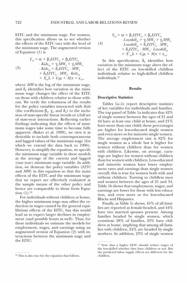
where MW is the log of the minimum wage, and d2 identifies how variation in the mini-mum wage changes the effect of the eITC on those with children relative to those with-out. We verify the robustness of the results for the policy variables interacted with Kids (the coefficients β2, γ2, and d2) to the inclu-sion of state-specific linear trends or a full set of state-year interactions. reflecting earlier findings indicating that the effects of mini-mum wages take some time to become fully apparent (baker et al. 1999), we view it as desirable to include both contemporaneous and lagged values of the minimum wage (for which we extend the data back to 1996). However, to simplify the equation, we specify the minimum wage variable in these models as the average of the current and lagged (one year) minimum wage variable. In addi-tion, we demean the policy variables (EITC and MW) in this equation so that the main effects of the eITC and the minimum wage that we report are effectively evaluated at the sample means of the other policy and hence are comparable to those from equa-tion (1).30

For individuals without children at home, the higher minimum wage may offset the re-duction in wages caused by the general equi-librium effects of the eITC, but this would lead us to expect larger declines in employ-ment (and possibly hours as well). Thus, for these individuals we estimate the models for employment, wages, and earnings using an augmented version of equation (2) with in-teractions between the minimum wage and the eITC:

30 This is also true for the equation that follows.

(4)

Yist 5 a 1 β1EITCst 1 β2 EITCst ⋅ Lowskillist 1 γ1MWst 1 γ2MWst ⋅ Lowskillist 1 d1EITCst ⋅ MWst 1 d2EITCst ⋅ MWst ⋅ Lowskillist 1 X 'ist λ 1 Gs m 1 Mt ν 1 εist .

In this specification, d2 identifies how variation in the minimum wage alters the ef-fect of the eITC on low-skilled childless individuals relative to high-skilled childless individuals.31

Results

Descriptive statistics

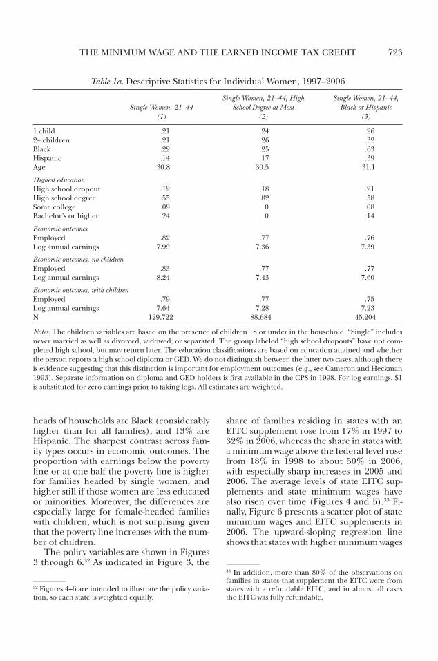
Tables 1a–1c report descriptive statistics of key variables for individuals and families. The top panel of Table 1a indicates that 42% of single women between the ages of 21 and 44 have at least one child at home, and 21% have more than one child; these percentages are higher for less-educated single women and even more so for minority single women. The average employment rate is 82% for single women as a whole but is higher for women without children than for women with children. likewise, on average, earn-ings are higher for women without children than for women with children. less-educated and minority women have lower employ-ment rates and earnings than single women overall; this is true for women both with and without children. Turning to childless men and women between the ages of 21 and 34, Table 1b shows that employment, wages, and earnings are lower for those with less educa-tion, and even more so for less-educated blacks and Hispanics.

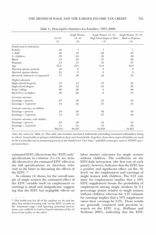
Finally, as Table 1c shows, 45% of all fami-lies are reported as female-headed, and 44% have two married spouses present. Among families headed by single women, which constitute 28% of families, 43% have chil-dren at home, implying that among all fami-lies with children, 24% are headed by single mothers. In addition, 23% of single women

31 Note that a higher eITC should reduce wages of the less-skilled whether they have children or not. but the predicted labor supply effects are different for the childless.

THe mINImum WAGe AND THe eArNeD INCome TAX CreDIT 723

heads of households are black (considerably higher than for all families), and 13% are Hispanic. The sharpest contrast across fam-ily types occurs in economic outcomes. The proportion with earnings below the poverty line or at one-half the poverty line is higher for families headed by single women, and higher still if those women are less educated or minorities. moreover, the differences are especially large for female-headed families with children, which is not surprising given that the poverty line increases with the num-ber of children.

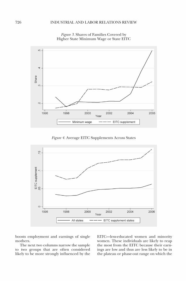
The policy variables are shown in Figures 3 through 6.32 As indicated in Figure 3, the

32 Figures 4–6 are intended to illustrate the policy varia-tion, so each state is weighted equally.

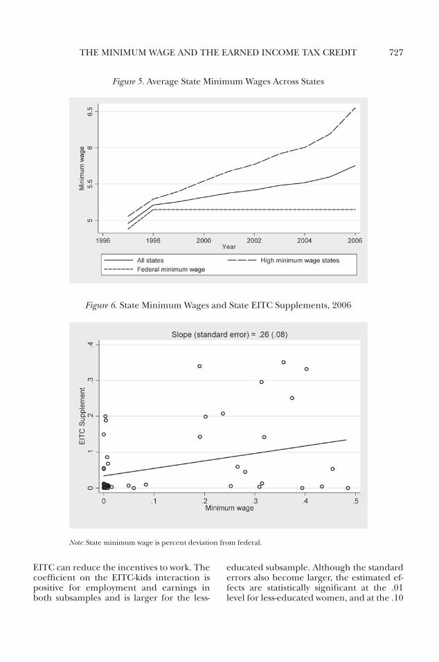
share of families residing in states with an eITC supplement rose from 17% in 1997 to 32% in 2006, whereas the share in states with a minimum wage above the federal level rose from 18% in 1998 to about 50% in 2006, with especially sharp increases in 2005 and 2006. The average levels of state eITC sup-plements and state minimum wages have also risen over time (Figures 4 and 5).33 Fi-nally, Figure 6 presents a scatter plot of state minimum wages and eITC supplements in 2006. The upward-sloping regression line shows that states with higher minimum wages

33 In addition, more than 80% of the observations on families in states that supplement the eITC were from states with a refundable eITC, and in almost all cases the eITC was fully refundable.

Table 1a. Descriptive Statistics for Individual Women, 1997–2006

Single Women, 21–44(1)

Single Women, 21–44, High School Degree at Most

(2)

Single Women, 21–44, Black or Hispanic

(3)

1 child .21 .24 .262+ children .21 .26 .32black .22 .25 .63Hispanic .14 .17 .39Age 30.8 30.5 31.1

Highest educationHigh school dropout .12 .18 .21High school degree .55 .82 .58Some college .09 0 .08bachelor’s or higher .24 0 .14

Economic outcomesemployed .82 .77 .76log annual earnings 7.99 7.36 7.39

Economic outcomes, no childrenemployed .83 .77 .77log annual earnings 8.24 7.43 7.60

Economic outcomes, with childrenemployed .79 .77 .75log annual earnings 7.64 7.28 7.23N 129,722 88,684 45,204

Notes: The children variables are based on the presence of children 18 or under in the household. “Single” includes never married as well as divorced, widowed, or separated. The group labeled “high school dropouts” have not com-pleted high school, but may return later. The education classifications are based on education attained and whether the person reports a high school diploma or GeD. We do not distinguish between the latter two cases, although there is evidence suggesting that this distinction is important for employment outcomes (e.g., see Cameron and Heckman 1993). Separate information on diploma and GeD holders is first available in the CPS in 1998. For log earnings, $1 is substituted for zero earnings prior to taking logs. All estimates are weighted.

INDuSTrIAl AND lAbor relATIoNS reVIeW724

tended to have a more generous eITC sup-plement. The considerable dispersion of points around the line indicates that states varied considerably in their use of these poli-cies, with some states implementing high minimum wages but low (or no) eITC sup-plements, and vice versa. This variation helps us to identify how the interaction of state minimum wages and state eITC supplements influenced economic outcomes for individu-als and families.

Regression Results: Individual Outcomes for Women

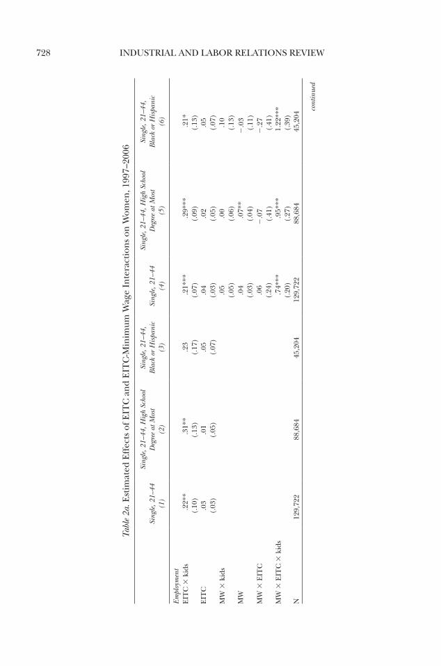
We begin with regression estimates of the effects of the eITC on the employment and earnings of single women between the ages of 21 and 44. The first three columns of Table 2a report the specifications with the eITC variables only, and the last three col-umns incorporate the eITC-minimum wage interactions. The table makes clear that the

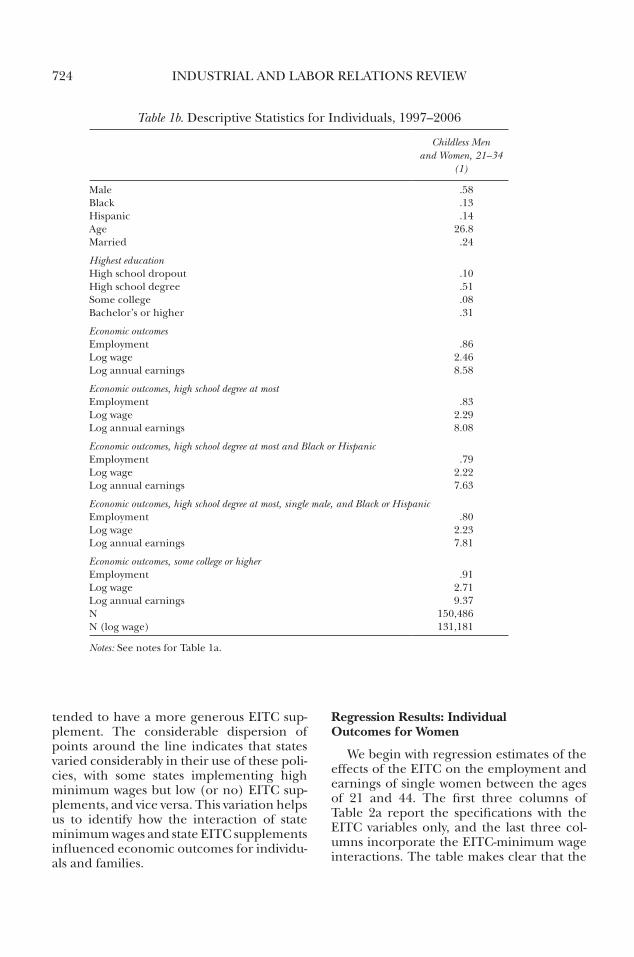
Table 1b. Descriptive Statistics for Individuals, 1997–2006

Childless Men and Women, 21–34

(1)

male .58black .13Hispanic .14Age 26.8married .24

Highest educationHigh school dropout .10High school degree .51Some college .08bachelor’s or higher .31

Economic outcomesemployment .86log wage 2.46log annual earnings 8.58

Economic outcomes, high school degree at most employment .83log wage 2.29log annual earnings 8.08

Economic outcomes, high school degree at most and Black or Hispanic employment .79log wage 2.22log annual earnings 7.63

Economic outcomes, high school degree at most, single male, and Black or Hispanic employment .80log wage 2.23log annual earnings 7.81

Economic outcomes, some college or higher employment .91log wage 2.71log annual earnings 9.37N 150,486N (log wage) 131,181

Notes: See notes for Table 1a.

THe mINImum WAGe AND THe eArNeD INCome TAX CreDIT 725

estimated eITC effects from the “eITC-only” specifications in columns (1)–(3) are virtu-ally identical to the estimated eITC effects in the full specifications; we therefore refer only to the latter in discussing the effects of the eITC. 34

As column (4) shows, for the overall sam-ple of single women the estimated effect of the eITC variable itself on employment or earnings is small and insignificant, suggest-ing that the eITC has negligible effects on

34 This holds true for all of the analyses we do and im-plies that studies focusing only on the eITC or only on the minimum wage—and ignoring potential interac-tions—are unlikely to lead to biased estimates of the ef-fects of one policy or the other.

labor market outcomes for single women without children. The coefficient on the eITC-kids interaction (the first row of each panel), however, indicates that the eITC has a positive and significant effect (at the .01 level) on the employment and earnings of single women with children. The 0.21 esti-mate for employment implies that a 10% eITC supplement boosts the probability of employment among single mothers by 2.1 percentage points relative to single women without children whereas the 2.21 estimate for earnings implies that a 10% supplement raises their earnings by 2.2%. These results are generally consistent with previous re-search on the eITC (e.g., Hoffman and Seidman 2003), indicating that the eITC

Table 1c. Descriptive Statistics for Families, 1997–2006

21–44 (1)

Single Women, 21–44

(2)

Single Women, 21–44, High School Degree at Most

(3)

Single Women, 21–44, Black or Hispanic

(4)

Family head or individualFemale .45 1 1 11 child .18 .19 .22 .232+ children .32 .24 .30 .36black .14 .23 .27 .66Hispanic .14 .13 .16 .37Age 33.4 32.1 31.9 32.3married, spouse present .44 0 0 0married, spouse absent .02 0 0 0Divorced, widowed, or separated .17 .38 .42 .33

Highest educationHigh school dropout .12 .12 .19 .22High school degree .50 .52 .81 .56Some college .09 .09 0 .08bachelor’s or higher .29 .26 0 .14

Economic outcomesearnings < poverty .19 .36 .45 .45earnings < .5∙poverty .12 .24 .31 .31

Economic outcomes, no childrenearnings < poverty .19 .26 .36 .32earnings < .5∙poverty .13 .19 .27 .24

Economic outcomes, with childrenearnings < poverty .19 .48 .54 .54earnings < .5∙poverty .11 .31 .35 .36N 362,811 98,327 65,839 34,267

Notes: See notes for Table 1a. This table also includes unrelated individuals (including unrelated subfamilies) living in others’ households or primary individuals in their own households. Together, these three types of families are used by the Census bureau in measuring poverty at the family level. (See http://pubdb3.census.gov/macro/032007/pov/povnotes.htm.)

INDuSTrIAl AND lAbor relATIoNS reVIeW726

boosts employment and earnings of single mothers.

The next two columns narrow the sample to two groups that are often considered likely to be more strongly influenced by the

eITC—less-educated women and minority women. These individuals are likely to reap the most from the eITC because their earn-ings are low and thus are less likely to be in the plateau or phase-out range on which the

Figure 3. Shares of Families Covered by Higher State minimum Wage or State eITC

Figure 4. Average eITC Supplements Across States

THe mINImum WAGe AND THe eArNeD INCome TAX CreDIT 727

eITC can reduce the incentives to work. The coefficient on the eITC-kids interaction is positive for employment and earnings in both subsamples and is larger for the less-

educated subsample. Although the standard errors also become larger, the estimated ef-fects are statistically significant at the .01 level for less-educated women, and at the .10

Figure 5. Average State minimum Wages Across States

Figure 6. State minimum Wages and State eITC Supplements, 2006

Note: State minimum wage is percent deviation from federal.

INDuSTrIAl AND lAbor relATIoNS reVIeW728

Tabl

e 2a

. est

imat

ed e

ffec

ts o

f eIT

C a

nd

eIT

C-m

inim

um W

age

Inte

ract

ion

s on

Wom

en, 1

997–

2006

Sing

le, 2

1–44

(1

)

Sing

le, 2

1–44

, Hig

h Sc

hool

D

egre

e at

Mos

t (2

)

Sing

le, 2

1–44

, B

lack

or

His

pani

c (3

)Si

ngle

, 21–

44

(4)

Sing

le, 2

1–44

, Hig

h Sc

hool

D

egre

e at

Mos

t (5

)

Sing

le, 2

1–44

, B

lack

or

His

pani

c (6

)

Empl

oym

ent

eIT

C 3

kid

s.2

2**

(.10

).3

1**

(.13

).2

3(.

17)

.21*

**(.

07)

.29*

**(.

09)

.21*

(.13

)e

ITC

.03

(.03

).0

1(.

05)

.05

(.07

).0

4(.

03)

.02

(.05

).0

5(.

07)

mW

3 k

ids

.05

(.05

).0

0(.

06)

.10

(.13

)m

W.0

4(.

03)

.07*

*(.

04)

2.0

3(.

11)

mW

3 e

ITC

.06

(.24

)2

.07

(.41

)2

.27

(.41

)m

W 3

eIT

C 3

kid

s.7

4***

(.20

).9

5***

(.27

)1.

22**

*(.

39)

N12

9,72

288

,684

45,2

0412

9,72

288

,684

45,2

04

cont

inue

d

THe mINImum WAGe AND THe eArNeD INCome TAX CreDIT 729

Log

ear

ning

se

ITC

3 k

ids

2.29

**(1

.01)

3.31

**(1

.33)

1.75

(1.8

5)2.

21**

*(.

69)

3.17

***

(.87

)1.

62(1

.25)

eIT

C.2

2(.

28)

2.0

8(.

51)

.63

(.95

).2

7(.

28)

2.0

3(.

51)

.64

(.82

)m

W 3

kid

s.6

0(.

49)

.30

(.58

)1.

16(1

.32)

mW

.38

(.31

).6

3*(.

38)

2.5

0(1

.12)

mW

3 e

ITC

.04

(2.3

1)2

.96

(3.5

8)2

4.38

(4.7

8)m

W 3

eIT

C 3

kid

s8.

30**

*(1

.84)

9.70

***

(2.5

1)14

.6**

*(4

.7)

N12

9,72

288

,684

45,2

0412

9,72

288

,684

45,2

04

Not

es: A

ll es

tim

ates

are

wei

ghte

d, a

nd

stan

dard

err

ors

are

clus

tere

d on

sta

tes.

Th

e m

inim

um w

age

vari

able

(m

W)

is t

he

aver

age

of t

he

log

of t

he

con

tem

pora

neo

us

and

lagg

ed m

inim

um w

age.

In

th

e m

inim

um w

age-

eIT

C in

tera

ctio

ns,

th

e m

inim

um w

age

and

eIT

C v

aria

bles

are

dem

ean

ed b

efor

e fo

rmin

g an

y in

tera

ctio

ns;

th

us,

the

non

-inte

ract

ed e

ITC

an

d m

inim

um w

age

coef

fici

ents

mea

sure

the

effe

cts

at th

e sa

mpl

e m

ean

of t

he

oth

er p

olic

y, a

nd

in p

arti

cula

r th

e e

ITC

coe

ffici

ents

in c

ol-

umn

s (4

)–(6

) h

ave

the

sam

e in

terp

reta

tion

(at

the

mea

ns)

as

thos

e in

col

umn

s (1

)–(3

). I

n th

e lo

g ea

rnin

gs s

peci

fica

tion

, $1

is s

ubst

itut

ed fo

r ze

ro e

arn

ings

pri

or to

ta

kin

g lo

gs. T

he

esti

mat

ed c

oeffi

cien

ts o

f th

e e

ITC

-kid

s, m

W-k

ids,

an

d e

ITC

-mW

-kid

s in

tera

ctio

ns

are

robu

st t

o in

clud

ing

stat

e-sp

ecifi

c lin

ear

tren

ds, o

r st

ate-

year

in

tera

ctio

ns;

in th

e la

tter

spe

cifi

cati

ons

the

mai

n e

ITC

eff

ect d

rops

out

. *S

tati

stic

ally

sig

nifi

can

t at t

he

.10

leve

l; **

at th

e .0

5 le

vel;

***a

t th

e .0

1 le

vel.

Tabl

e 2a

. est

imat

ed e

ffec

ts o

f eIT

C a

nd

eIT

C-m

inim

um W

age

Inte

ract

ion

s on

Wom

en, 1

997–

2006

Con

tin

ued

Sing

le, 2

1–44

(1

)

Sing

le, 2

1–44

, Hig

h Sc

hool

D

egre

e at

Mos

t (2

)

Sing

le, 2

1–44

, B

lack

or

His

pani

c (3

)Si

ngle

, 21–

44

(4)

Sing

le, 2

1–44

, Hig

h Sc

hool

D

egre

e at

Mos

t (5

)

Sing

le, 2

1–44

, B

lack

or

His

pani

c (6

)

INDuSTrIAl AND lAbor relATIoNS reVIeW730

level (for employment only) for minority women.

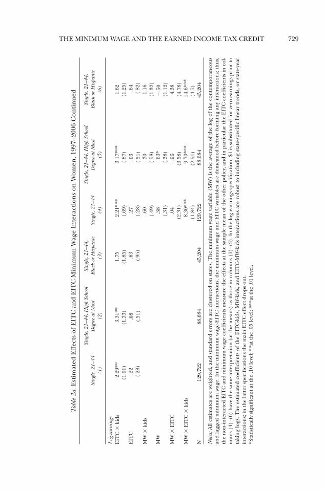
Next, we turn to the minimum wage-eITC interactions. recall that for women who are eligible for the eITC, the disemployment ef-fects of a higher minimum wage could partly offset the positive employment effect of the eITC. Alternatively, the interaction for these women could be positive, because a higher minimum wage makes the eITC more valu-able for eligible families. In contrast, for groups not likely to be eligible for the eITC (or eligible for only a small credit), a high minimum wage coupled with an eITC could be a particularly bad combination, with the minimum wage reducing their employment prospects via the higher wage floor imposed on employers and the eITC reducing their employment prospects via the in-creased supply of eligible women entering the labor market. For single women and families, this latter effect pertains to child-less women and thus would be captured by the coefficient on the eITC-minimum wage interaction. (For childless low-skilled indi-viduals, discussed next, this latter effect would be captured by the triple interaction between the eITC, the minimum wage, and the low-skill indicator.)

In the employment regressions shown in columns (4)–(6) of Table 2a, the estimated interaction term between the minimum wage, the eITC, and children is positive and significant for all three groups of single women, indicating that a higher minimum wage amplifies the positive labor supply re-sponse of the eITC for single mothers. The results are stronger for less-educated and minority mothers (columns (5) and (6)). In contrast, for single women without children, the coefficient on the eITC-mini-mum wage interaction is near zero and is not significant, and it is negative for mi-norities and less-educated women. The coef-ficients in the earnings regressions are consistent with the results for employment. The minimum wage-eITC interaction has a positive and significant effect on the earn-ings of women with children, with larger ef-fects evident for minority or less-educated women. And again, for minority and less- educated women without children, the

interaction is negative, albeit not statistically significant.35

These results suggest that the combina-tion of an eITC and a higher minimum wage may be especially powerful in raising the em-ployment and earnings of low-skilled single mothers.36 However, the estimates also hint at the possibility that the positive labor sup-ply response of single mothers eligible for the eITC may reduce employment and earn-ings among low-educated or minority single women without children. We present more direct analyses of these spillover effects below.

Table 2b presents the evidence in a man-ner that makes it easier to interpret the pre-ceding results.37 In particular, the table reports implied effects of various policy com-binations on employment, which for women is the outcome that is the common focus of

35 Although we do not report the results in the tables, we verified that these key results are robust to more flexible specifications that include either state-specific time trends or a full set of state-by-year interactions. This is true for the other analyses that follow as well, as indi-cated in the notes to the appropriate tables. 36 Although not shown in the table, we also estimated these models for log wages and for hours conditional on working. For wages, the coefficient on the interac-tion between the eITC and the minimum wage vari-ables was negative and sometimes statistically significant for single women without children, suggesting a nega-tive spillover onto the wages of those women earning more than the minimum wage. In contrast, there was little evidence of spillovers to the wages of women with children, although this may reflect selection bias associ-ated with the decision regarding whether to work. For hours, there was some evidence that a higher minimum wage coupled with an eITC supplement led to reduc-tions in conditional hours for minority women without children, which may reflect the same spillover effects that reduce wages for these women. Finally, the esti-mated effects of the eITC on employment, hours, and earnings were negative (but insignificant) for married women with children, and who have at most a high school education. These findings parallel those in eissa and Hoynes (2004), although eissa and Hoynes some-times found statistically stronger evidence that the eITC reduces labor market participation of less-educated married women.37 The eITC variable is in the 0.05 to 0.35 range, and the minimum wage is in logs. Thus, for example, the inter-active effect of a 10% increase in the minimum wage and a 0.1 increase in the eITC supplement is 0.01 times the interactive coefficient. These small magnitudes can make the regression coefficients in Table 2a a bit diffi-cult to interpret.

THe mINImum WAGe AND THe eArNeD INCome TAX CreDIT 731

Table 2b. Implied effect on employment of 10% State eITC Supplement on Single Women at Different minimum Wage levels, based on

estimates of Interactive Specifications in Table 2a

Single Female, 21–44(1)

Single Female, 21–44, High School Degree at Most

(2)

Single Female, 21–44, Black or Hispanic

(3)

At sample mean of minimum wageWith children .025***

(.008).031***

(.010).026**

(.010)Childless .004

(.003).002

(.005).005

(.007)Difference .021***

(.007).029***

(.009).021*

(.013)

Minimum wage 10% higherWith children .033***

(.010).040***

(.012).036***

(.012)Childless .004

(.005).001

(.008).002

(.008)Difference .029***

(.008).039***

(.009).034**

(.013)

Difference relative to effect at mean minimum wage With children .008**

(.003).009***

(.003).010***

(.003)Childless .001

(.002)2.001(.004)

2.003(.004)

Difference .007***(.002)

.010***(.003)

.012***(.004)

Minimum wage 25% higher With children .045***

(.014).053***

(.016).050***

(.015)Childless .005

(.008).000

(.014)2.002(.012)

Difference .040***(.009)

.053***(.011)

.052***(.016)

Difference relative to effect at mean minimum wage With children .020**

(.008).022***

(.008).024***

(.006)Childless .001

(.006)2.002(.010)

2.007(.010)

Difference .018***(.005)

.024***(.007)

.031***(.010)

Notes: t-statistics are the same by construction for the calculation of differences relative to the mean minimum wage using the minimum wage 10% or 25% above the sample mean. The estimated differences are robust to including state-year interactions in which only the differences are identified. See notes for Table 2a.

research on the effects of the eITC. For ex-ample, the first column of the table shows the effect of introducing a 10% state eITC supplement on the employment status of single women under three different values

of the minimum wage—a wage floor set at the sample mean (first panel), a minimum wage set 10% above the sample mean (sec-ond panel), and a minimum wage set 25% above the sample mean (fourth panel). As

INDuSTrIAl AND lAbor relATIoNS reVIeW732

the top panel indicates, introducing a 10% eITC supplement in a state where the mini-mum wage is set to the sample average leads to a statistically significant increase in em-ployment among single women with chil-dren but has little effect on the employment of childless women. With a higher minimum wage (second and fourth panels), the effects of the eITC on the employment of single mothers become more strongly positive, whereas the effects on the employment of single women without children are essen-tially unchanged. The difference in the re-sponses of women with and without children to the eITC is statistically significant at the .01 level in all cases (first, second, and fourth panels), and the change in the relative re-sponse of women with children when the minimum wage is raised is always significant at the .01 level (third and fifth panels). Thus, these comparisons clearly indicate that the eITC and the minimum wage interact in a way that induces a larger absolute and rela-tive labor supply response among women with children when the minimum wage is high.

The remaining two columns show corre-sponding effects for low-skilled and minority single women. For these two samples, the es-timated employment effects for single women with children are again larger than for the sample of all single women, and they rise more steeply with increases in the minimum wage. The results are nearly as strong statistically. As in the first column, the differences in the interactions between the eITC and the minimum wage for single women with and without children are significantly different in these samples and suggest that a higher minimum wage boosts the positive effects of the eITC on the em-ployment of women with children, who are more likely to be eligible for generous eITC payments.

Regression Results: Outcomes for Low-skilled, childless Individuals and teenagers

The positive labor supply response to the eITC of eligible mothers may lead to nega-tive spillover effects on other less-skilled in-

dividuals who are “ineligible” for the eITC but who compete for jobs with the new labor force entrants. Table 3a presents evidence on these spillovers for several different groups of such individuals for wages, em-ployment, and earnings. In this specifica-tion, we identify the effect of the eITC from an interaction between the eITC supple-ment and an indicator for low skills, which we define as having at most a high school de-gree. To focus in on those individuals more likely to be substitutes in production for women benefiting from the eITC, we limit the sample to childless men and women be-tween the ages of 21 and 34. We first estimate the model for all individuals in this age range. We then restrict the treatment group to less-skilled minorities, and finally to less-skilled minority single men, keeping the control group the same in each case.38 This last treatment group is of interest for at least two reasons. First, single men may be less skilled or less productive than otherwise comparable married men (e.g., Korenman and Neumark 1991). Second, single, less-skilled, and especially minority men have been the focus of policy proposals regarding extensions of the eITC (e.g., Gitterman et al. 2007).

As in Table 2a, the estimated eITC ef-fects from the “eITC-only” specifications in

38 We maintain the larger control group as we narrow the treatment group for two reasons. First, a control group that consisted of only blacks and Hispanics would be very small, because of the lower average edu-cation levels of those groups. For example, in columns (2) and (5), the control group (for the employment and earnings regressions) would decline from 57,581 to 9,818, and in columns (3) and (6) it would decline to 3,522, resulting in estimates that are often less precise. Second, we were concerned that control groups consisting of minorities would be more prone to biases resulting from some minorities being affected by the treatment. That is, it seems reasonable to assume that only a small share of White, black, or Hispanic, single or married, college-educated individuals is affected by the eITC, whereas a greater share of black or Hispanic, single, college-educated individuals may be affected, given that minorities are more heavily concentrated in the lower part of the wage distribution. That said, the key results for minimum wage-eITC interactions using the narrower control groups are similar to those re-ported in Table 3a. These results are available upon re-quest by writing to the first author.

THe mINImum WAGe AND THe eArNeD INCome TAX CreDIT 733

Tabl

e 3a

. est

imat

ed e

ffec

ts o

f eIT

C a

nd

eIT

C-m

inim

um W

age

Inte

ract

ion

s on

l

ow-S

kille

d, C

hild

less

In

divi

dual

s, A

ged

21–3

4, 1

997–

2006

Low

-Ski

lled

Trea

tmen

t G

roup

Les

s-Edu

cate

d

Indi

vidu

als

(1)

Les

s-Edu

cate

d B

lack

or

His

pani

c (2

)

Les

s-Edu

cate

d Si

ngle

B

lack

or

His

pani

c M

en

(3)

Les

s-Edu

cate

d

Indi

vidu

als

(4)

Les

s-Edu

cate

d B

lack

or

His

pani

c (5

)

Les

s-Edu

cate

d Si

ngle

B

lack

or

His

pani

c M

en

(6)

Log

wag

ese

ITC

3 lo

w-s

kill

2.1

0(.

09)

2.1

1(.

08)

2.1

3(.

09)

2.0

9(.

09)

2.1

1(.

07)

2.1

3(.

08)

eIT

C.0

8(.

07)

.06

(.10

).0

8(.

11)

.09*

(.05

).0

7(.

06)

.09

(.07

)m

W 3

low

-ski

ll2

.04

(.04

)2

.13*

*(.

06)

2.1

7**

(.07

)m

W.1

5***

(.05

).1

7**

(.07

).1

5*(.

08)

mW

3 e

ITC

21.

08**

*(.

26)

21.

09**

*(.

30)

21.

06 *

**(.

31)

mW

3 e

ITC

3

low

-ski

ll.6

2*(.

34)

.45

(.72

).1

1(.

99)

N13

1,18

179

,362

67,3

9913

1,18

179

,362

67,3

99

Empl

oym

ent

eIT

C 3

low

-ski

ll2

.05

(.05

)2

.12*

*(.

05)

2.1

6***

(.05

)2

.04

(.05

)2

.12*

**(.

04)

2.1

6***

(.05

)e

ITC

.02

(.04

).0

3(.

03)

.01

(.03

).0

3(.

03)

.04

(.02

).0

2(.

03)

mW

3 lo

w-s

kill

2.0

1(.

02)

.07*

*(.

03)

.09*

**(.

03)

mW

.06*

**(.

02)

.02

(.02

).0

0(.

03)

mW

3 e

ITC

2.1

1(.

11)

2.0

6(.

09)

2.0

1(.

10)

mW

3 e

ITC

3

low

-ski

ll2

.26

(.17

)2

.78*

**(.

23)

2.8

9***

(.25

)N

150,

486

90,4

0874

,913

150,

486

90,4

0874

,913 co

ntin

ued

INDuSTrIAl AND lAbor relATIoNS reVIeW734

Log

ear

ning

se

ITC

3 lo

w-s

kill

2.5

8(.

49)

21.

32**

*(.

44)

21.

75**

*(.

56)

2.5

4(.

49)

21.

32**

*(.

39)

21.

74**

*(.

48)

eIT

C.3

5(.

38)

.40

(.37

).3

5(.

29)

.40

(.27

).4

9*(.

25)

.44

(.29

)m

W 3

low

-ski

ll2

.15

(.15

).6

3**

(.27

).9

1***

(.33

)m

W.7

3***

(.20

).2

5(.

17)

.11

(.24

)m

W 3

eIT

C2

1.95

*(.

99)

21.

32(.

94)

2.9

1(1

.09)

mW

3 e

ITC

3

low

-ski

ll2

1.90

(1.7

7)2

7.65

***

(2.7

9)2

8.69

***

(2.7

0)

N15

0,48

690

,408

74,9

1315

0,48

690

,408

74,9

13

Not

es: S

ee n

otes

for

Tab

le 2

a. T

he

log

wag

e re

gres

sion

s co

ndi

tion

on

pos

itiv

e ea

rnin

gs a

nd

hou

rs o

f w

ork

in t

he

prev

ious

yea

r. “l

ess-

educ

ated

” m

ean

s th

at t

he

indi

-vi

dual

has

a h

igh

sch

ool d

egre

e at

mos

t. T

he

low

-ski

lled

trea

tmen

t gro

up is

defi

ned

in th

e co

lum

n h

eadi

ng.

Th

e co

ntr

ol g

roup

doe

s n

ot c

han

ge a

cros

s co

lum

ns

and

alw

ays

incl

udes

all

thos

e w

ith

at l

east

som

e co

llege

(re

gard

less

of r

ace,

eth

nic

ity,

or

mar

ital

sta

tus)

. Th

e es

tim

ated

coe

ffici

ents

of t

he

eIT

C-lo

w-s

kill,

mW

-low

-ski

ll, a

nd

eIT

C-m

W-lo

w-s

kill

inte

ract

ion

s ar

e ro

bust

to in

clud

ing

stat

e-sp

ecifi

c lin

ear

tren

ds, o

r st

ate-

year

inte

ract

ion

s.

Tabl

e 3a

. est

imat

ed e

ffec

ts o

f eIT

C a

nd

eIT

C-m

inim

um W

age

Inte

ract

ion

s on

l

ow-S

kille

d, C

hild

less

In

divi

dual

s, A

ged

21–3

4, 1

997–

2006

Con

tin

ued

Low

-Ski

lled

Trea

tmen

t G

roup

Les

s-Edu

cate

d

Indi

vidu

als

(1)

Les

s-Edu

cate

d B

lack

or

His

pani

c (2

)

Les

s-Edu

cate

d Si

ngle

B

lack

or

His

pani

c M

en

(3)

Les

s-Edu

cate

d

Indi

vidu

als

(4)

Les

s-Edu

cate

d B

lack

or

His

pani

c (5

)

Les

s-Edu

cate

d Si

ngle

B

lack

or

His

pani

c M

en

(6)

THe mINImum WAGe AND THe eArNeD INCome TAX CreDIT 735

eITC could put additional downward pres-sure on wages for those earning more than the minimum wage. on the other hand, a high minimum wage could create a floor below which wages cannot fall despite the increased labor supply of women, in which case the combined policies might reduce employment more strongly. As the results in the table indicate, the evidence is more con-sistent with the latter type of effect. Although the point estimates of the effects of the eITC on low-skilled wages are negative, there is no evidence that this adverse effect is com-pounded by a higher minimum wage; the es-timated interactive coefficients for low-skilled childless individuals are positive and gener-ally insignificant.40 In contrast, the point esti-mates of the triple interaction (mW × eITC × low-skill) for employment are negative for all three treatment groups and are larger and statistically significant when we focus on minorities and single males (in columns (5) and (6)); these results imply that a higher minimum wage exacerbates the adverse ef-fects of the eITC on the employment on these individuals. Finally, as the lower panel indicates, the presence of either an eITC or a minimum wage tends to reduce the rela-tive earnings of the low-skilled, and these ef-fects are heightened when both policies are in effect—with a statistically significant inter-action evident for blacks or Hispanics and the narrower subgroup of minority single males.

In Table 3b, we present the implied ef-fects of a range of policy combinations on the earnings of childless individuals, similar to the exercise shown in Table 2b. In this case, we differentiate between the effects of policy on the earnings of lower-skilled/ minority and higher-skilled individuals. As the top panel indicates, the combination of a 10% eITC supplement and a minimum wage set at its sample mean leads to a small loss in earnings among the low-skilled,

40 As noted above, leigh (2010) also estimated a specifi-cation for unskilled wages that included an interaction between the eITC and the minimum wage. Consistent with our results, he found that a higher minimum wage did little to influence the effects of the eITC on the wages of low-skilled workers.

columns (1)–(3) are virtually identical to the estimated eITC effects in the full specifica-tions (columns (4)–(6)), and so we refer only to the latter in discussing the effects of the eITC. For less-educated, childless indi-viduals (column (4)), the estimated eITC effects on wages, employment, and earnings are negative, although none of these is statis-tically significant. However, for less-educated blacks and Hispanics (column (5)), the esti-mated effects of the eITC on employment and earnings are negative and statistically significant, and the point estimates are larger than those in column (4), indicating that this group is adversely affected by the eITC. The estimated effect on wages is also nega-tive, but not significant. Finally, as indicated in column (6), the results for less-educated single minority men are stronger than those in column (5), with the estimates pointing to negative effects of the eITC on wages, em-ployment, and earnings; the estimates for the latter two outcomes are statistically significant.39

These columns also report results for the minimum wage-eITC interactions. In prin-ciple, a higher minimum wage coupled with an eITC could affect this group of individu-als in at least two ways. on the one hand, a high minimum wage that leads to more labor market entry among women eligible for the

39 We estimated similar specifications for hours condi-tional on employment, which are available upon re-quest by writing to the first author. The estimated eITC effects on the hours of low-skilled individuals were neg-ative for all three treatment groups, although statisti-cally significant only for the sample corresponding to column (4). In addition, we estimated models for each of the dependent variables using only the low-skilled subsample, which entails dropping the interactions in equation (2). In this case, all of the estimated eITC ef-fects were near zero and statistically insignificant, sug-gesting that the use of the high-skilled group as a control helps to capture other economic shocks across states and years. We want to note, however, that leigh (2010) reported wage regression estimates for a sample of low-skilled individuals that are consistent with the predicted negative effects of the eITC on the unskilled, although the sample period and specification differ in other ways. rothstein (2008) explored this issue more fully in the context of federal increases in the eITC in the 1990s, noting the importance of controlling for demand shifts to detect the adverse effects of the eITC on wages.

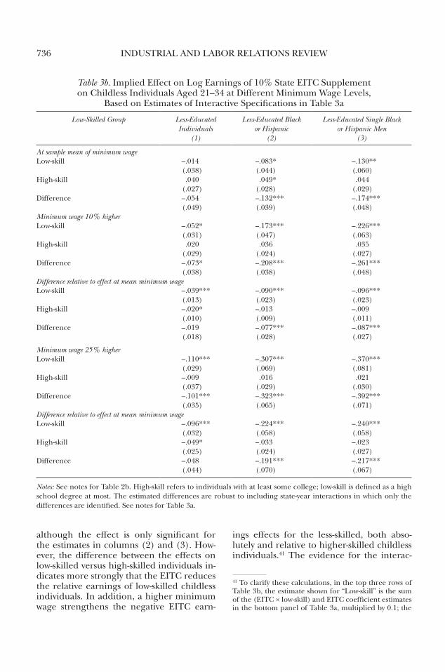
INDuSTrIAl AND lAbor relATIoNS reVIeW736

although the effect is only significant for the estimates in columns (2) and (3). How-ever, the difference between the effects on low-skilled versus high-skilled individuals in-dicates more strongly that the eITC reduces the relative earnings of low-skilled childless individuals. In addition, a higher minimum wage strengthens the negative eITC earn-

ings effects for the less-skilled, both abso-lutely and relative to higher-skilled childless individuals.41 The evidence for the interac-

41 To clarify these calculations, in the top three rows of Table 3b, the estimate shown for “low-skill” is the sum of the (eITC × low-skill) and eITC coefficient estimates in the bottom panel of Table 3a, multiplied by 0.1; the

Table 3b. Implied effect on log earnings of 10% State eITC Supplement on Childless Individuals Aged 21–34 at Different minimum Wage levels,

based on estimates of Interactive Specifications in Table 3a

Low-Skilled Group Less-Educated Individuals

(1)

Less-Educated Black or Hispanic

(2)

Less-Educated Single Black or Hispanic Men

(3)

At sample mean of minimum wagelow-skill –.014

(.038)–.083*(.044)

–.130**(.060)

High-skill .040(.027)

.049*(.028)

.044(.029)

Difference –.054(.049)

–.132***(.039)

–.174***(.048)

Minimum wage 10% higherlow-skill –.052*

(.031)–.173***(.047)

–.226***(.063)

High-skill .020(.029)

.036(.024)

.035(.027)

Difference –.073*(.038)

–.208***(.038)

–.261***(.048)

Difference relative to effect at mean minimum wage low-skill –.039***

(.013)–.090***(.023)

–.096***(.023)

High-skill –.020*(.010)

–.013(.009)

–.009(.011)

Difference –.019(.018)

–.077***(.028)

–.087***(.027)

Minimum wage 25% higher low-skill –.110***

(.029)–.307***(.069)

–.370***(.081)

High-skill –.009(.037)

.016(.029)

.021(.030)

Difference –.101***(.035)

–.323***(.065)

–.392***(.071)

Difference relative to effect at mean minimum wage low-skill –.096***

(.032)–.224***(.058)

–.240***(.058)

High-skill –.049*(.025)

–.033(.024)

–.023(.027)

Difference –.048(.044)

–.191***(.070)

–.217***(.067)

Notes: See notes for Table 2b. High-skill refers to individuals with at least some college; low-skill is defined as a high school degree at most. The estimated differences are robust to including state-year interactions in which only the differences are identified. See notes for Table 3a.

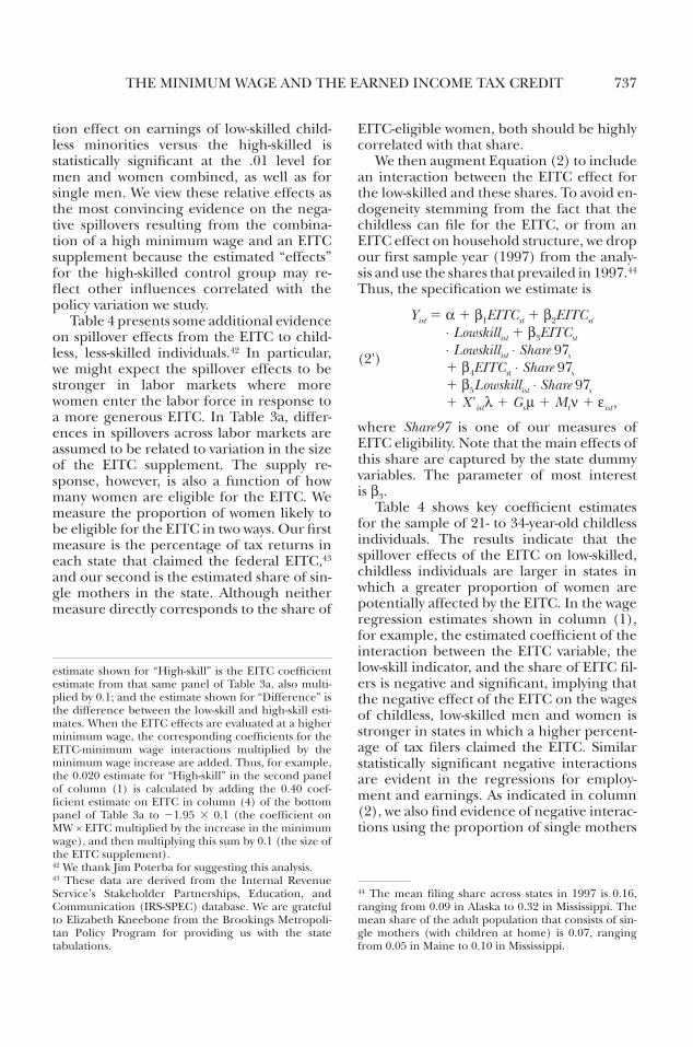
THe mINImum WAGe AND THe eArNeD INCome TAX CreDIT 737

tion effect on earnings of low-skilled child-less minorities versus the high-skilled is statistically significant at the .01 level for men and women combined, as well as for single men. We view these relative effects as the most convincing evidence on the nega-tive spillovers resulting from the combina-tion of a high minimum wage and an eITC supplement because the estimated “effects” for the high-skilled control group may re-flect other influences correlated with the policy variation we study.

Table 4 presents some additional evidence on spillover effects from the eITC to child-less, less-skilled individuals.42 In particular, we might expect the spillover effects to be stronger in labor markets where more women enter the labor force in response to a more generous eITC. In Table 3a, differ-ences in spillovers across labor markets are assumed to be related to variation in the size of the eITC supplement. The supply re-sponse, however, is also a function of how many women are eligible for the eITC. We measure the proportion of women likely to be eligible for the eITC in two ways. our first measure is the percentage of tax returns in each state that claimed the federal eITC,43 and our second is the estimated share of sin-gle mothers in the state. Although neither measure directly corresponds to the share of

estimate shown for “High-skill” is the eITC coefficient estimate from that same panel of Table 3a, also multi-plied by 0.1; and the estimate shown for “Difference” is the difference between the low-skill and high-skill esti-mates. When the eITC effects are evaluated at a higher minimum wage, the corresponding coefficients for the eITC-minimum wage interactions multiplied by the minimum wage increase are added. Thus, for example, the 0.020 estimate for “High-skill” in the second panel of column (1) is calculated by adding the 0.40 coef-ficient estimate on eITC in column (4) of the bottom panel of Table 3a to 21.95 3 0.1 (the coefficient on mW × eITC multiplied by the increase in the minimum wage), and then multiplying this sum by 0.1 (the size of the eITC supplement).42 We thank Jim Poterba for suggesting this analysis. 43 These data are derived from the Internal revenue Service’s Stakeholder Partnerships, education, and Communication (IrS-SPeC) database. We are grateful to elizabeth Kneebone from the brookings metropoli-tan Policy Program for providing us with the state tabulations.

eITC-eligible women, both should be highly correlated with that share.

We then augment equation (2) to include an interaction between the eITC effect for the low-skilled and these shares. To avoid en-dogeneity stemming from the fact that the childless can file for the eITC, or from an eITC effect on household structure, we drop our first sample year (1997) from the analy-sis and use the shares that prevailed in 1997.44 Thus, the specification we estimate is

(2')

Yist 5 a 1 β1EITCst 1 β2EITCst ⋅ Lowskillist 1 β3EITCst ⋅ Lowskillist ⋅ Share 97s 1 β4EITCst ⋅ Share 97s 1 β5Lowskillist ⋅ Share 97s 1 X 'ist λ 1 Gs m 1 Mt ν 1 εist ,

where Share97 is one of our measures of eITC eligibility. Note that the main effects of this share are captured by the state dummy variables. The parameter of most interest is β3.

Table 4 shows key coefficient estimates for the sample of 21- to 34-year-old childless individuals. The results indicate that the spillover effects of the eITC on low-skilled, childless individuals are larger in states in which a greater proportion of women are potentially affected by the eITC. In the wage regression estimates shown in column (1), for example, the estimated coefficient of the interaction between the eITC variable, the low-skill indicator, and the share of eITC fil-ers is negative and significant, implying that the negative effect of the eITC on the wages of childless, low-skilled men and women is stronger in states in which a higher percent-age of tax filers claimed the eITC. Similar statistically significant negative interactions are evident in the regressions for employ-ment and earnings. As indicated in column (2), we also find evidence of negative interac-tions using the proportion of single mothers

44 The mean filing share across states in 1997 is 0.16, ranging from 0.09 in Alaska to 0.32 in mississippi. The mean share of the adult population that consists of sin-gle mothers (with children at home) is 0.07, ranging from 0.05 in maine to 0.10 in mississippi.

INDuSTrIAl AND lAbor relATIoNS reVIeW738

in the state as the share variable.45 The evi-dence that the effects of the eITC are more adverse when a larger share of the popula-tion is potentially affected by the eITC

45 The estimates of the eITC-share interaction effect on conditional hours, for which the theoretical prediction is ambiguous, were also negative, but not significant, in both specifications. We also estimated these models for the other subsamples considered in Table 3a. The quali-tative conclusions based on the point estimates were fairly similar, with one exception: For low-skilled minor-ities, the point estimates did not suggest that a higher share filing or a higher share of single mothers is associ-ated with sharper negative effects of the eITC on wages. This may reflect the lower wages of minorities, implying that more of them are bound by the minimum wage so that the wage cannot decline as much in response to the labor supply increases induced by the eITC.

strengthens the conclusion that we are de-tecting spillover effects of the eITC.

Teenagers are another group for which the combination of a high minimum wage and an eITC may produce adverse effects. Previous researchers have found evidence of substitutability between women and youth (e.g., Grant and Hamermesh 1981), raising the possibility that an eITC-induced outward supply shift for women with children may de-press labor market opportunities for teenag-ers. As for other groups, this substitutability could lead to downward pressure on wages or reduced employment.

To investigate this possibility, we estimate, for 16- to 19-year-old males and females, models that, similar to those presented above, allow for interactions between the

Table 4. estimated eITC effects on low-Skilled (less-educated), Childless Individuals, Aged 21–34, Variation with Share Affected by eITC, 1998–2006

Using Share Filing for EITC (1)

Using Share of Single Mothers (2)

Log wageseITC 3 low-skill –.22***

(.05)–.05(.04)

eITC .09(.08)

.01(.07)

eITC 3 low-skill 3 1997 filing/single mother share (3 10)

–.38**(.15)

–.84**(.34)

N 120,976 120,976

EmploymenteITC × low-skill –.14***

(.01)–.04** (.02)

eITC –.02(.05)

–.03(.04)

eITC 3 low-skill 3 1997 filing/single mother share (3 10)

–.21***(.06)

–.55***(.15)

N 139,096 139,096

Log earningseITC 3 low-skill –1.54***

(.16)–.43**(.18)

eITC –.03(.53)

–.19(.48)

eITC 3 low-skill 3 1997 filing/single mother share (3 102)

–.23***(.07)

–.60***(.16)

N 139,096 139,096

Notes: See notes to Table 3a. The sample corresponds to columns (1) and (4) of that table, so the low-skill indicator in this table refers to the less-educated. Data from 1997 are omitted; estimates corresponding to Table 3a excluding 1997 were very similar to estimates in Table 3a. The filing or single mother share in the interaction is demeaned, so the eITC 3 low-skill coefficient measures the relative effect of the eITC on the low-skilled at the mean of the corre-sponding share.

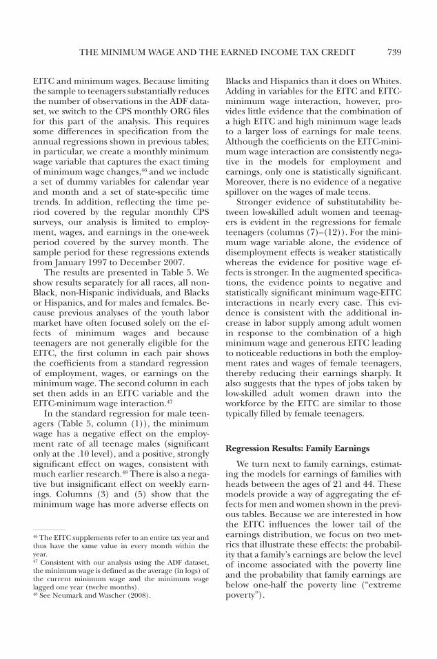
THe mINImum WAGe AND THe eArNeD INCome TAX CreDIT 739

eITC and minimum wages. because limiting the sample to teenagers substantially reduces the number of observations in the ADF data-set, we switch to the CPS monthly orG files for this part of the analysis. This requires some differences in specification from the annual regressions shown in previous tables; in particular, we create a monthly minimum wage variable that captures the exact timing of minimum wage changes,46 and we include a set of dummy variables for calendar year and month and a set of state-specific time trends. In addition, reflecting the time pe-riod covered by the regular monthly CPS surveys, our analysis is limited to employ-ment, wages, and earnings in the one-week period covered by the survey month. The sample period for these regressions extends from January 1997 to December 2007.

The results are presented in Table 5. We show results separately for all races, all non-black, non-Hispanic individuals, and blacks or Hispanics, and for males and females. be-cause previous analyses of the youth labor market have often focused solely on the ef-fects of minimum wages and because teenagers are not generally eligible for the eITC, the first column in each pair shows the coefficients from a standard regression of employment, wages, or earnings on the minimum wage. The second column in each set then adds in an eITC variable and the eITC-minimum wage interaction.47

In the standard regression for male teen-agers (Table 5, column (1)), the minimum wage has a negative effect on the employ-ment rate of all teenage males (significant only at the .10 level), and a positive, strongly significant effect on wages, consistent with much earlier research.48 There is also a nega-tive but insignificant effect on weekly earn-ings. Columns (3) and (5) show that the minimum wage has more adverse effects on

46 The eITC supplements refer to an entire tax year and thus have the same value in every month within the year.47 Consistent with our analysis using the ADF dataset, the minimum wage is defined as the average (in logs) of the current minimum wage and the minimum wage lagged one year (twelve months).48 See Neumark and Wascher (2008).

blacks and Hispanics than it does on Whites. Adding in variables for the eITC and eITC-minimum wage interaction, however, pro-vides little evidence that the combination of a high eITC and high minimum wage leads to a larger loss of earnings for male teens. Although the coefficients on the eITC-mini-mum wage interaction are consistently nega-tive in the models for employment and earnings, only one is statistically significant. moreover, there is no evidence of a negative spillover on the wages of male teens.

Stronger evidence of substitutability be-tween low-skilled adult women and teenag-ers is evident in the regressions for female teenagers (columns (7)–(12)). For the mini-mum wage variable alone, the evidence of disemployment effects is weaker statistically whereas the evidence for positive wage ef-fects is stronger. In the augmented specifica-tions, the evidence points to negative and statistically significant minimum wage-eITC interactions in nearly every case. This evi-dence is consistent with the additional in-crease in labor supply among adult women in response to the combination of a high minimum wage and generous eITC leading to noticeable reductions in both the employ-ment rates and wages of female teenagers, thereby reducing their earnings sharply. It also suggests that the types of jobs taken by low-skilled adult women drawn into the workforce by the eITC are similar to those typically filled by female teenagers.

Regression Results: Family earnings

We turn next to family earnings, estimat-ing the models for earnings of families with heads between the ages of 21 and 44. These models provide a way of aggregating the ef-fects for men and women shown in the previ-ous tables. because we are interested in how the eITC influences the lower tail of the earnings distribution, we focus on two met-rics that illustrate these effects: the probabil-ity that a family’s earnings are below the level of income associated with the poverty line and the probability that family earnings are below one-half the poverty line (“extreme poverty”).

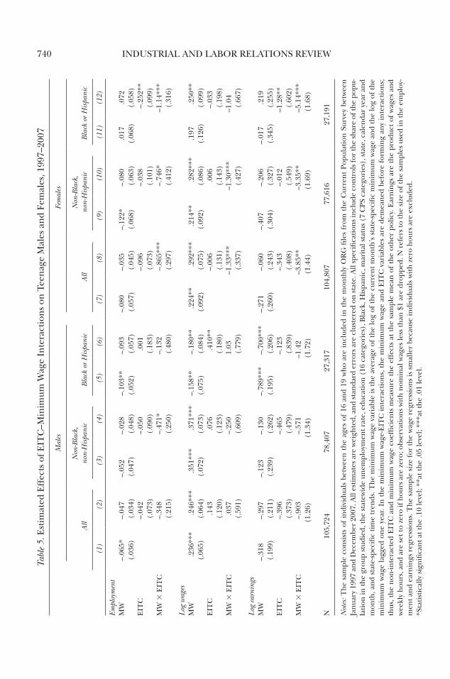
INDuSTrIAl AND lAbor relATIoNS reVIeW740Ta

ble

5. e

stim

ated

eff

ects

of e

ITC

–min

imum

Wag

e In

tera

ctio

ns

on T

een

age

mal

es a

nd

Fem

ales

, 199

7–20

07

Mal

esFe

mal

es

All

Non

-Bla

ck,

non-

His

pani

cB

lack

or

His

pani

cA

llN

on-B

lack

, no

n-H

ispa

nic

Bla

ck o

r H

ispa

nic

(1)

(2)

(3)

(4)

(5)

(6)

(7)

(8)

(9)

(10)

(11)

(12)

Empl

oym

ent

mW

–.06

5*(.

036)

–.04

7(.

034)

–.05

2(.

047)

–.02

8(.

048)

–.10

3**

(.05

2)–.

093

(.05

7)–.

080

(.05

7)–.

035

(.04

5)–.

122*

(.06

8)–.

080

(.06

3).0

17(.

068)

.072

(.05

8)e

ITC

–.04

2(.

073)

–.05

0(.

090)

.001

(.18

3)–.

096

(.07

3)–.

038

(.10

1)–.

252*

*(.

099)

mW

3 e

ITC

–.34

8(.

215)

–.47

1*(.

250)

–.13

2(.

480)

–.86

5***

(.29

7)–.

746*

(.41

2)–1

.14*

**(.

316)

Log

wag

esm

W.2

36**

*(.

065)

.246

***

(.06

4).3

51**

*(.

072)

.371

***

(.07

3)–.

158*

*(.

075)

–.18

0**

(.08

4).2

24**

(.09

2).2

92**

*(.

075)

.214

**(.

092)

.282

***

(.08

6).1

97(.

126)

.250

**(.

099)

eIT

C.1

43(.

120)

.076

(.12

3).4

10**

(.18

0)–.

006

(.13

1).0

06(.

143)

–.03

3(.

198)

mW

3 e

ITC

.037

(.59

1)–.

250

(.60

9)1.

03(.

779)

–1.3

3***

(.33

7)–1

.30*

**(.

427)

–1.0

4(.

667)

Log

ear

ning

sm

W–.

318

(.19

9)–.

297

(.21

1)–.

123

(.23

9)–.

130

(.26

2)–.

789*

**(.

195)

–.70

0***

(.20

6)–.

271

(.26

0)–.

060

(.24

3)–.

407

(.30

4)–.

206

(.32

7)–.

017

(.34

5).2

19(.

255)

eIT

C–.

396

(.37

3)–.

465

(.47

9)–.

123

(.83

9)–.

343

(.40

8)–.

012

(.54

9)–1

.28*

*(.

602)

mW

3 e

ITC

–.90

3(1

.26)

–.57

1(1

.34)

–1.4

2(1

.72)

–3.8

5**

(1.4

4)–3

.35*

*(1

.69)

–5.1

4***

(1.6

8)

N10

5,72

478

,407

27,3

1710

4,80

777

,616

27,1

91

Not

es:

Th

e sa

mpl

e co

nsi

sts

of i

ndi

vidu

als

betw

een

th

e ag

es o

f 16

an

d 19

wh

o ar

e in

clud

ed i

n t

he

mon

thly

or

G fi

les

from

th

e C

urre

nt

Popu

lati

on S

urve

y be

twee

n

Jan

uary

199

7 an

d D

ecem

ber

2007

. All

esti

mat

es a

re w

eigh

ted,

an

d st

anda

rd e

rror

s ar

e cl

uste

red

on s

tate

. All

spec

ifica

tion

s in

clud

e co

ntr

ols

for

the

shar

e of

the

popu

-la

tion

in th

e gr

oup

stud

ied,

the

stat

ewid

e un

empl

oym

ent r

ate,

edu

cati

on (

16 c

ateg

orie

s), b

lack

, His

pan

ic, m

arit

al s

tatu

s (7

CPS

cat

egor

ies)

, sta

te, c

alen

dar

year

an

d m

onth

, an

d st

ate-

spec

ific

tim

e tr

ends

. Th

e m

inim

um w

age

vari

able

is t

he

aver

age

of t

he

log

of t

he

curr

ent

mon

th’s

sta

te-s

peci

fic

min

imum

wag

e an

d th

e lo

g of

th

e m

inim

um w

age

lagg

ed o

ne

year

. In

th

e m

inim

um w

age-

eIT

C in

tera

ctio

ns,

th

e m

inim

um w

age

and

eIT

C v

aria

bles

are

dem

ean

ed b

efor

e fo

rmin

g an

y in

tera

ctio

ns;

th

us, t

he

non

-inte

ract

ed e

ITC

an

d m

inim

um w

age

coef

fici

ents

mea

sure

th

e ef

fect

s at

th

e sa

mpl

e m

ean

of

the

oth

er p

olic

y. e

arn

ings

are

th

e pr

oduc

t of

wag

es a

nd

wee

kly

hou

rs, a

nd

are

set t

o ze

ro if

hou

rs a

re z

ero;

obs

erva

tion

s w

ith

nom

inal

wag

es le

ss th

an $

1 ar

e dr

oppe

d. N

ref

ers

to th

e si

ze o

f th

e sa

mpl

es u

sed

in th

e em

ploy

-m

ent a

nd

earn

ings

reg

ress

ion

s. T

he

sam

ple

size

for

the

wag

e re

gres

sion

s is

sm

alle

r be

caus

e in

divi

dual

s w

ith

zer

o h

ours

are

exc

lude

d.*S

tati

stic

ally

sig

nifi

can

t at t

he

.10

leve

l; **

at th

e .0

5 le

vel;

***a

t th

e .0

1 le

vel.

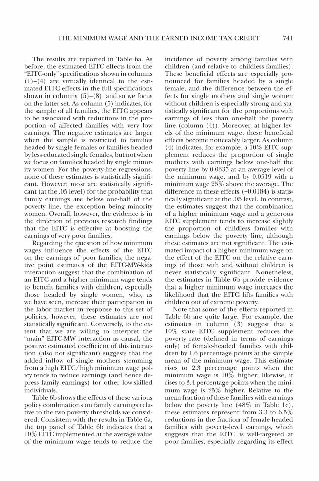
THe mINImum WAGe AND THe eArNeD INCome TAX CreDIT 741

The results are reported in Table 6a. As before, the estimated eITC effects from the “eITC-only” specifications shown in columns (1)–(4) are virtually identical to the esti-mated eITC effects in the full specifications shown in columns (5)–(8), and so we focus on the latter set. As column (5) indicates, for the sample of all families, the eITC appears to be associated with reductions in the pro-portion of affected families with very low earnings. The negative estimates are larger when the sample is restricted to families headed by single females or families headed by less-educated single females, but not when we focus on families headed by single minor-ity women. For the poverty-line regressions, none of these estimates is statistically signifi-cant. However, most are statistically signifi-cant (at the .05 level) for the probability that family earnings are below one-half of the poverty line, the exception being minority women. overall, however, the evidence is in the direction of previous research findings that the eITC is effective at boosting the earnings of very poor families.

regarding the question of how minimum wages influence the effects of the eITC on the earnings of poor families, the nega-tive point estimates of the eITC-mW-kids interaction suggest that the combination of an eITC and a higher minimum wage tends to benefit families with children, especially those headed by single women, who, as we have seen, increase their participation in the labor market in response to this set of policies; however, these estimates are not statistically significant. Conversely, to the ex-tent that we are willing to interpret the “main” eITC-mW interaction as causal, the positive estimated coefficient of this interac-tion (also not significant) suggests that the added inflow of single mothers stemming from a high eITC/high minimum wage pol-icy tends to reduce earnings (and hence de-press family earnings) for other low-skilled individuals.

Table 6b shows the effects of these various policy combinations on family earnings rela-tive to the two poverty thresholds we consid-ered. Consistent with the results in Table 6a, the top panel of Table 6b indicates that a 10% eITC implemented at the average value of the minimum wage tends to reduce the

incidence of poverty among families with children (and relative to childless families). These beneficial effects are especially pro-nounced for families headed by a single female, and the difference between the ef-fects for single mothers and single women without children is especially strong and sta-tistically significant for the proportions with earnings of less than one-half the poverty line (column (4)). moreover, at higher lev-els of the minimum wage, these beneficial effects become noticeably larger. As column (4) indicates, for example, a 10% eITC sup-plement reduces the proportion of single mothers with earnings below one-half the poverty line by 0.0335 at an average level of the minimum wage, and by 0.0519 with a minimum wage 25% above the average. The difference in these effects (−0.0184) is statis-tically significant at the .05 level. In contrast, the estimates suggest that the combination of a higher minimum wage and a generous eITC supplement tends to increase slightly the proportion of childless families with earnings below the poverty line, although these estimates are not significant. The esti-mated impact of a higher minimum wage on the effect of the eITC on the relative earn-ings of those with and without children is never statistically significant. Nonetheless, the estimates in Table 6b provide evidence that a higher minimum wage increases the likelihood that the eITC lifts families with children out of extreme poverty.

Note that some of the effects reported in Table 6b are quite large. For example, the estimates in column (3) suggest that a 10% state eITC supplement reduces the poverty rate (defined in terms of earnings only) of female-headed families with chil-dren by 1.6 percentage points at the sample mean of the minimum wage. This estimate rises to 2.3 percentage points when the minimum wage is 10% higher; likewise, it rises to 3.4 percentage points when the mini-mum wage is 25% higher. relative to the mean fraction of these families with earnings below the poverty line (48% in Table 1c), these estimates represent from 3.3 to 6.5% reductions in the fraction of female-headed families with poverty-level earnings, which suggests that the eITC is well-targeted at poor families, especially regarding its effect

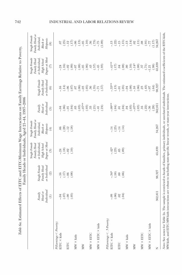
INDuSTrIAl AND lAbor relATIoNS reVIeW742Ta

ble

6a. e

stim

ated

eff

ects

of e

ITC

an

d e

ITC

-min

imum

Wag

e In

tera

ctio

ns

on F

amily

ear

nin

gs r

elat

ive

to P

over

ty,

Fam

ily H

eads

or

Indi

vidu

als,

Age

d 21

–44,

199

7–20

06

Fam

ily

Hea

d or

In

divi

dual

(1

)

Sing

le F

emal

e

Fam

ily H

ead

or

Ind

ivid

ual

(2)

Sing

le F

emal

e

Fam

ily H

ead

or

Ind

ivid

ual,

H

igh

Scho

ol

Deg

ree

at M

ost

(3)

Sing

le F

emal

e

Fam

ily H

ead

or

Indi

vidu

al,

Bla

ck o

r

His

pani

c

(4)

Fam

ily

Hea

d or

In

divi

dual

(5

)

Sing

le F

emal

e

Fam

ily H

ead

or

Ind

ivid

ual

(6)

Sing

le F

emal

e Fa

mily

Hea

d

or I

ndiv

idua

l,

Hig

h Sc

hool

D

egre

e at

Mos

t (7

)

Sing

le F

emal

e

Fam

ily H

ead

or

Indi

vidu

al,

Bla

ck o

r

His

pani

c

(8)

P(Ea

rnin

gs ,

Pov

erty

)e

ITC

3 k

ids

–.04

(.07

)–.

16(.

17)

–.24

(.18

).0

6(.

28)

–.04

(.06

)–.

16(.

14)

–.24

(.16

).0

7(.

25)

eIT

C–.

00(.

05)

–.06

(.08

)–.

02(.

10)

–.12

(.18

)–.

01(.

04)

–.06

(.07

)–.

02(.

09)

–.12

(.17

)m

W 3

kid

s.0

3(.

03)

.07

(.06

)–.

07(.

08)

–.06

(.13

)m

W–.

07**

(.03

)–.

03(.

05)

–.05

(.06

)–.

05(.

10)

mW

3 e

ITC

.33

(.21

).3

6(.

35)

.43

(.57

).3

6(.

73)

mW

3 e

ITC

3 k

ids

–.41

(.24

)–.

71(.

57)

–.45

(.93

)–.

75(1

.09)

P(Ea

rnin

gs ,

.5∙P

over

ty)

eIT

C 3

kid

s–.

09(.

06)

–.34

*(.

18)

–.42

*(.

23)

–.14

(.25

)–.

09**

(.04

)–.

33**

(.13

)–.

41**

(.17

)–.

13(.

22)

eIT

C.0

2(.

04)

.00

(.06

).0

5(.

09)

–.14

(.14

).0

1(.

04)

–.01

(.05

).0

4(.

08)

–.15

(.15

)m

W 3

kid

s.0

4(.

03)

–.04

(.08

).0

0(.

10)

–.13

(.14

)m

W–.

07**

(.03

)–.

10(.

06)

–.14

*(.

08)

.02

(.11

)m

W 3

eIT

C.1

6(.

22)

.23

(.43

).3

7(.

71)

.08

(.91

)m

W 3

eIT

C 3

kid

s–.

36(.

28)

–.97

(.64

)–1

.21

(.98

)–.

77(1

.17)

N36

2,81

198

,327

65,8

3934

,267

362,

811

98,3

2765

,839

34,2

67

Not

es: S

ee n

otes

for

Tabl

e 2a

. Th

e sa

mpl

e is

res

tric

ted

to h

eads

of f

amili

es, p

rim

ary

indi

vidu

als,

or

unre

late

d in

divi

dual

s. T

he

esti

mat

ed c

oeffi

cien

ts o

f th

e e

ITC

-kid

s,

mW

-kid

s, a

nd

eIT

C-m

W-k

ids

inte

ract

ion

s ar

e ro

bust

to in

clud

ing

stat

e-sp

ecifi

c lin

ear

tren

ds, o

r st

ate-

year

inte

ract

ion

s.

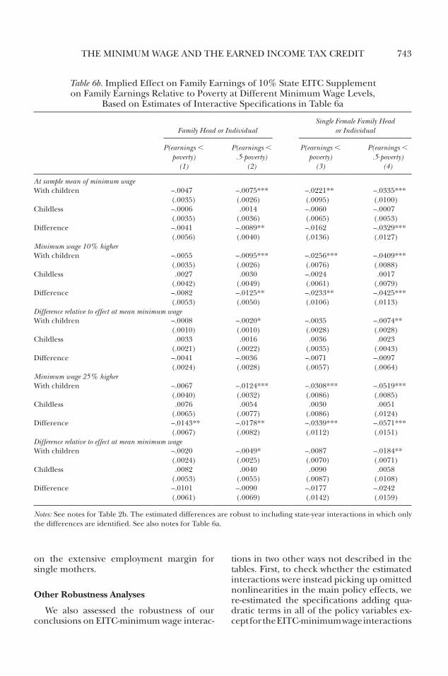
THe mINImum WAGe AND THe eArNeD INCome TAX CreDIT 743

Table 6b. Implied effect on Family earnings of 10% State eITC Supplement on Family earnings relative to Poverty at Different minimum Wage levels,

based on estimates of Interactive Specifications in Table 6a

Family Head or IndividualSingle Female Family Head

or Individual

P(earnings , poverty)

(1)

P(earnings , .5⋅poverty)

(2)

P(earnings , poverty)

(3)

P(earnings , .5⋅poverty)

(4)

At sample mean of minimum wageWith children –.0047

(.0035)–.0075***(.0026)

–.0221**(.0095)

–.0335***(.0100)

Childless –.0006(.0035)

.0014(.0036)

–.0060(.0065)

–.0007(.0053)

Difference –.0041(.0056)

–.0089**(.0040)

–.0162(.0136)

–.0329***(.0127)

Minimum wage 10% higherWith children –.0055

(.0035)–.0095***(.0026)

–.0256***(.0076)

–.0409***(.0088)

Childless .0027(.0042)

.0030(.0049)

–.0024(.0061)

.0017(.0079)

Difference –.0082(.0053)

–.0125**(.0050)

–.0233**(.0106)

–.0425***(.0113)

Difference relative to effect at mean minimum wage With children –.0008

(.0010)–.0020*(.0010)

–.0035(.0028)

–.0074**(.0028)

Childless .0033(.0021)

.0016(.0022)

.0036(.0035)

.0023(.0043)

Difference –.0041(.0024)

–.0036(.0028)

–.0071(.0057)

–.0097(.0064)

Minimum wage 25% higher With children –.0067

(.0040)–.0124***(.0032)

–.0308***(.0086)

–.0519***(.0085)

Childless .0076(.0065)

.0054(.0077)

.0030(.0086)

.0051(.0124)

Difference –.0143**(.0067)

–.0178**(.0082)

–.0339***(.0112)

–.0571***(.0151)

Difference relative to effect at mean minimum wage With children –.0020

(.0024)–.0049*(.0025)

–.0087(.0070)

–.0184**(.0071)

Childless .0082(.0053)

.0040(.0055)

.0090(.0087)

.0058(.0108)

Difference –.0101(.0061)

–.0090(.0069)

–.0177(.0142)

–.0242(.0159)

Notes: See notes for Table 2b. The estimated differences are robust to including state-year interactions in which only the differences are identified. See also notes for Table 6a.

on the extensive employment margin for single mothers.

Other Robustness Analyses

We also assessed the robustness of our conclusions on eITC-minimum wage interac-

tions in two other ways not described in the tables. First, to check whether the estimated interactions were instead picking up omitted nonlinearities in the main policy effects, we re-estimated the specifications adding qua-dratic terms in all of the policy variables ex-cept for the eITC-minimum wage interactions

INDuSTrIAl AND lAbor relATIoNS reVIeW744

(including in equation (3), for example, the main policy effects as well as their interac-tion with the dummy variable for children in the home). The estimated eITC-minimum wage interactions were quite similar, and the evidence was in some cases statistically stron-ger. Second, to check whether our identifica-tion was coming from the linear restrictions on the main and interactive effects, we cre-ated four indicators for each policy, with the first designating state/years for which no policy (or in the case of the minimum wage, a minimal policy) was in effect and the latter three designating state/years with low, me-dium, and high versions of the policy (roughly the eighth, ninth, and tenth deciles, in which the variation in policy occurs). We then estimated models with the full set of in-dicators and interactions corresponding to equations (3) and (4). In all cases, we still found evidence that higher minimum wages enhance the effects of the eITC for women and families, although sometimes this evi-dence only emerged over particular ranges of the eITC (e.g., the minimum wage en-hanced the effect of a “medium” eITC rela-tive to no eITC).

conclusions

The introduction of eITC supplements and higher minimum wages at the state level have noticeably altered the low-wage labor market since the mid-1990s. In this paper, we have shown how this combination of policies has influenced work incentives and labor market outcomes for various groups of low-skilled individuals and have examined the concomitant effects on the economic well-being of families. We first developed a simple theoretical framework that illustrates the ways in which minimum wages and the eITC could interact and showed that such interac-tions could differentially affect various groups.49 Specifically, we showed that a

49 We have framed this discussion in terms of how varia-tion in the minimum wage alters the effects of the eITC, mainly because this is how the policy argument is often couched. of course, an interaction between the two policies in a regression model can just as well be inter-

higher minimum wage can enhance the ef-fect of the eITC for women by inducing par-ticular subgroups to increase their willingness to work to a greater extent than would the eITC alone. At the same time, it is possible for an eITC coupled with a high minimum wage to have adverse effects, especially on low-skilled adults or teenagers who may have to compete with the women who are drawn into the labor market by the eITC. We thus estimated models that allow for interactions between minimum wages and the eITC to assess the relevance of these possibilities.

our findings confirm earlier research in-dicating that the eITC is an effective means of encouraging work among less-skilled sin-gle mothers. We also find that the eITC in-teracts with the minimum wage in a way that amplifies the labor supply response and in-crease in earnings among single women with children in the home, suggesting that the combination of an eITC and higher mini-mum wage can provide an additional boost to the incomes of such families. Conversely, our results also indicate that interactions be-tween the eITC and minimum wages lead to adverse effects on the employment and earn-ings of less-skilled and minority individuals without children in the home, which sug-gests that the benefits afforded to single women come at a cost, with minimum wages exacerbating the potentially adverse effects of the eITC on low-skilled individuals not eligible for the eITC.

Whether the policy combination of a high eITC and a high minimum wage is viewed as favorable or unfavorable ultimately depends on whose earnings or incomes policymakers are targeting. The distributional goals of public policy typically focus more on family income than on individual income; thus, it seems fair to say that policymakers have been most concerned with increasing resources for families with children, via the eITC, wel-fare, and other policies. However, the recent policy debate has also refocused attention on those without children in the home, and in particular on the low-skilled men who, ac-

preted as how a higher eITC influences the effects of the minimum wage.

THe mINImum WAGe AND THe eArNeD INCome TAX CreDIT 745

cording to our estimates, are hit especially hard by a combination of a high eITC and a high minimum wage. For example, in sup-port of an expansion in the eITC for those without children, berlin (2007) argued that policies aimed at raising labor market par-ticipation among less-skilled men might re-duce the relative attractiveness of illicit sources of income as well as make these men more attractive marriage partners, which would help to reverse the declines in mar-riage and increases in out-of-wedlock child-bearing and childrearing that have occurred in recent decades.50 In addition, Gitterman et al. (2007) pointed out that many men who are non-custodial parents still have financial responsibility for their children. These argu-ments suggest that policymakers should not

50 our estimates do not speak directly to this alternative type of eITC. However, the evidence of adverse effects of the present eITC on low-skilled individuals without children also suggests that a substantially more gener-ous eITC for those without children could pose nega-tive tradeoffs with respect to the women whose employment and earnings are boosted by the eITC as it is currently structured.

focus solely on how policies affect the earn-ings of low-skilled women or the income of female-headed families with children.

The evidence of policy interactions be-tween the eITC and the minimum wage also indicates that research on the distributional effects of one policy in isolation may be too narrow. As one example, we noted earlier in the paper that existing research does not find beneficial distributional effects of the minimum wage. However, this research did not consider policy interactions, and in our review of this work (Neumark and Wascher 2008), we suggested that the distributional effects of minimum wages may vary with the institutional and policy setting. Indeed, the evidence for interactive effects between the eITC and the minimum wage points to just one of a number of possible avenues by which changes in welfare and incentives to work since the mid-1990s may have altered the effects of the minimum wage. These avenues merit further study. And, of course, the question can be turned around to ex-tend the question we study, asking how other policy changes may have influenced the ef-fectiveness of the eITC.

ReFeReNces

baker, michael, Dwayne benjamin, and Shuchita Stanger. 1999. “The Highs and lows of the minimum Wage effect: A Time-Series Cross-Section Study of the Canadian law.” Journal of Labor Economics, Vol. 17, No. 2, pp. 318–50.

berlin, Gordon l. 2007. “rewarding the Work of Indi-viduals: A Counterintuitive Approach to reducing Poverty and Strengthening Families.” The Future of Children, Vol. 17, No. 2, pp. 17–42.

bernstein, Jared. 2004. rev. of Helping Working Families: The Earned Income Tax Credit by Saul D. Hoffman and laurence S. Seidman [Kalamazoo, mI: W.e. upjohn Institute for employment research, 2003]. Social Service Review, Vol. 78, No. 1, pp. 153–57.

bertrand, marianne, esther Duflo, and Sendhil mullainathan. 2004. “How much Should We Trust Differences-in-Differences estimators.” Quarterly Jour-nal of Economics, Vol. 119, No. 1, pp. 249–75.

berube, Alan, Ann Kim, benjamin Forman, and megan burns. 2002. “The Price of Paying Taxes: How Tax Preparation and refund loan Fees erode the bene-fits of the eITC.” Washington, D.C.: brookings Institu-tion and Progressive Policy Institute.

bingley, Paul, and Ian Walker. 2008. “The labor Supply effect of In-Kind Transfers.” unpublished paper, uni-versity of Warwick.

blank, rebecca m., and lucie Schmidt. 2001. “Work, Wages, and Welfare.” In rebecca m. blank and ron Haskins, eds., The New World of Welfare, pp. 70–102. Washington, DC: The brookings Institution.

burkhauser, richard V., Kenneth A. Couch, and An-drew J. Glenn. 1996. “Public Policies for the Working Poor: The earned Income Tax Credit Versus the mini-mum Wage.” Research in Labor Economics, Vol. 15, pp. 65–109.

Cameron, Stephen, and James J. Heckman. 1993. “The Nonequivalence of High School equivalents.” Journal of Labor Economics, Vol. 11, No. 1, Pt. 1, pp. 1–47.

Cancian, maria, and Arik levinson. 2005. “labor Sup-ply effects of the earned Income Tax Credit: evidence from Wisconsin’s Supplemental benefit for Families with Three Children.” Nber Working Paper No. 11454.

economic Policy Institute. 2004. “The minimum Wage and earned Income Tax Credit: Partners in making Work Pay.” retrieved from <http://www.epinet.org/content.cfm/webfeatures_snapshots_05052004>.

INDuSTrIAl AND lAbor relATIoNS reVIeW746

eissa, Nada, and Jeffrey liebman. 1996. “labor Supply response to the earned Income Tax Credit.” Quarterly Journal of Economics, Vol. 112, No. 2, pp. 605–37.

____, and Hilary Williamson Hoynes. 2004. “Taxes and the labor market Participation of married Couples: The earned Income Tax Credit.” Journal of Public Eco-nomics, Vol. 88, No. 9–10, pp. 1931–58.

Fiscal Policy Institute. 2004. “State minimum Wages and employment in Small businesses.” Fiscal Policy Insti-tute, New York, NY.

Gitterman, Daniel P., lucy S. Gorham, and Jessica l. Dorrance. 2007. “expanding the eITC for Single Workers and Couples Without Children (aka Tax re-lief for low-Wage Workers).” unpublished paper, university of North Carolina–Chapel Hill.

Grant, James H., and Daniel S. Hamermesh. 1981. “labor market Competition among Youths, White Women, and others.” Review of Economics and Statistics, Vol. 63, No. 3, pp. 354–60.

Grogger, Jeffrey. 2003. “The effects of Time limits, the eITC, and other Policy Changes on Welfare use, Work, and Income among Female-Headed Families.” Review of Economics and Statistics, Vol. 85, No. 2, pp. 394–408.

Hoffman, Saul D., and laurence S. Seidman. 2003. Helping Working Families: The Earned Income Tax Credit. Kalamazoo, mI: W.e. upjohn Institute for employ-ment research.

Hotz, V. Joseph, and John Karl Scholz. 2003. “The earned Income Tax Credit.” In robert A. moffitt, ed. Means-Tested Transfer Programs in the United States, pp. 141–97. Chicago: university of Chicago Press.

Korenman, Sanders and David Neumark. 1991. “Does marriage really make men more Productive?” Journal of Human Resources, Vol. 26, No. 2, pp. 282–307.

leigh, Andrew. 2005. “Who benefits from the earned Income Tax Credit? Incidence Among recipi-ents, Coworkers, and Firms.” The Australian National university Centre for economic Policy research, Dis-cussion Paper No. 494.

____. 2010. “Who benefits from the earned Income Tax Credit? Incidence Among recipients, Coworkers, and Firms.” The B.E. Journal of Economic Analysis and Policy, Vol. 10, No. 1, pp. 1–41.

levitis, Jason A., and Nicholas Johnson. 2006. “To-gether, State minimum Wages and State earned In-

come Tax Credits make Work Pay.” Center on Budget and Policy Priorities. retrieved from <http://www.cbpp.org/7–12–06sfp.htm>.

liebman, Jeffrey b. 1998. “The Impact of the earned Income Tax Credit on Incentives and the Income Dis-tribution.” In James Poterba, ed. Tax Policy and the Economy, Vol. 12, pp. 83–120. Cambridge, mA: mIT Press.

machin, Stephen, and Alan manning. 1994. “minimum Wages, Wage Dispersion and employment: evidence from the uK Wages Councils.” Industrial and Labor Re-lations Review, Vol. 47, No. 2, pp. 319–29.

manning, Alan. 2003. Monopsony in Motion: Imperfect Competition in Labor Markets. Princeton: Princeton uni-versity Press.

meyer, bruce. 2002. “labor Supply at the extensive and Intensive margins: The eITC, Welfare, and Hours Worked.” American Economic Review, Vol. 92, No. 2, pp. 373–79.

Neumark, David, and William Wascher. 1996. “The ef-fects of minimum Wages on Teenage employment and enrollment: estimates from matched CPS Data.” Research in Labor Economics, Vol. 15, pp. 25–64.

____, and ____. 2001. “using the eITC to Help Poor Families: New evidence and a Comparison with the minimum Wage.” National Tax Journal, Vol. 54, No. 2, pp. 281–318.

____, and ____. 2007a. “minimum Wages and employ-ment.” Foundations and Trends in Microeconomics, Vol. 3, Nos. 1–2, pp. 1–186.

____, and ____. 2007b. “minimum Wages, the earned Income Tax Credit, and employment: evidence from the Post-Welfare reform era.” Nber Working Paper No. 12915.

____, and ____. 2008. Minimum Wages. Cambridge, mA: mIT Press.

romich, Jennifer l., and Thomas Weisner. 2000. “How Families View and use the eITC: Advance Payment versus lump Sum Delivery.” National Tax Journal, Vol. 53, No. 4, Pt. 2, pp. 1245–66.

rothstein, Jesse. 2008. “The unintended Consequences of encouraging Work: Tax Incidence and the eITC.” unpublished paper, Princeton university.

Scholz, John Karl. 1994. “The earned Income Tax Credit: Participation, Compliance, Antipoverty effec-tiveness.” National Tax Journal, Vol. 47, No. 1, pp. 63–87.