Embed Size (px)
Citation preview

`
COMBINING MINIMUM WAGE
AND EARNED INCOME TAX CREDIT
POLICIES TO GUARANTEE A
DECENT LIVING STANDARD TO
ALL U.S. WORKERS
Jeannette Wicks-Lim &
Jeffrey Thompson
Political Economy Research Institute
University of Massachusetts, Amherst
October 2010
Combining Minimum Wage and Earned Income Tax Credit Policies to Guarantee a Decent Living Standard to All U.S. Workers
Jeannette Wicks-Lim & Jeffrey Thompson Political Economy Research Institute
University of Massachusetts Amherst
October 2010

TABLE OF CONTENTS
Summary 1
Introduction 3
Background 7
Can a Minimum Wage be a Living Wage? 15
Can the EITC Fill the Gap Between a High Minimum Wage & the Decent Living Income Standard? 31
The Other Half of the Challenge: Getting to Full Employment 41
Conclusion 43
Technical Appendices 45
References 58
SUMMARY
This study advances proposals to substantially strengthen minimum wage laws and the federal Earned Income Tax Credit (EITC) program in the United States, so that, in combination, they can guarantee decent living standards for all full-time U.S. workers and their families. By considering minimum wage laws and the EITC as complements, we show how these measures can operate most effectively to achieve this guarantee and, crucially, how any possible negative unintended consequences of each measure can be minimized.
Specifically, we begin by proposing a 70 percent increase in current minimum wage rates. This would raise the federal minimum from today’s rate of $7.25 to $12.30 per hour. We also propose two expansions of the EITC, the federal program that provides tax relief and cash benefits for low-income working families. These include raising the maximum EITC benefits by 80 percent and the income eligibility threshold to three times the federal poverty line. The maximum EITC benefit would rise from $5,028 to $9,040 and households with incomes up to $57,000 could receive some benefit.
In combination, these two policy measures would guarantee 60 percent of all low-income working families a decent living standard through full-time employment. The other 40 percent of low-income working families offer more difficult challenges, because they either live in high-cost areas or they depend on only one wage-earner to raise children. But our proposed measures would substantially improve conditions for these households as well. Current policy terms guarantee a decent living standard for only 12 percent of low-income working families.
By strengthening both the minimum wage and EITC in combination, we take advantage of how they can operate in complementary ways—that is, with the strengths of one policy making up for the weaknesses of the other. The minimum wage, if raised too high, could cause business costs to rise significantly and in response, employers could potentially lay off workers or cut back on their hours. The EITC program has the advantage of supplementing the earnings of low-income workers without raising business costs. Generous EITC benefits, however, tend to draw more people into the labor force and allow employers to pay less while still attracting the workers they need. A robust minimum wage rate would prevent wages from falling too low due to the EITC. Finally, federal budget constraints limit how large EITC benefits can be.
We crafted our proposals by first establishing a key measure, which we term the “minimum wage tipping point.” The minimum wage tipping point is reached when business cost increases exceed the capacity of businesses to absorb these costs while maintaining the same level of employment. Of course, there will be some level of the minimum wage at which such a tipping point is reached. Our bias in seeking to identify this tipping point has been, if anything, to err on the low side in our interpretation of the evidence. We do not want to suggest that that virtually any plausible minimum wage increase could be implemented without creating negative employment effects. Nevertheless, based on our cautious interpretation of the evidence, we conclude, once the U.S. economy is recovering from the Great Recession, that the current minimum wage of $7.25 could be raised by 70 percent, to $12.30 per hour, before causing any significant negative employment effects—that is, before hitting the tipping point.
Two factors combine to make a 70 percent minimum wage hike fall below the tipping point in a growing U.S. economy. The first is that the cost increases of minimum wage hikes for businesses tend to be relatively modest, as a share of their overall costs. In addition, firms are able to adjust to the cost increases resulting from a higher minimum wage through various measures other than layoffs or cutting
Wicks-Lim & Thompson / Combining Minimum Wage and EITC Policies to Guarantee a Decent Living Standard to All U.S. Workers / October 2010 / page 1
back workers’ hours. These adjustments include 1) raising prices; 2) improving productivity; 3) reducing profits and 4) expanding firm operations in conjunction with the normal pace of economic growth.
A 70 percent increase lifts the minimum wage to a “living wage” for about 72 percent of low-income families residing in states with low-to-average living costs. The remaining 28 percent of low-income working households are those with only one adult worker raising at least one child. Additionally, families living in high-cost areas will need more support than those in the typical state to cover their family budgets. We turn to the EITC program to help close these remaining gaps.
The current terms of the federal EITC program do not raise low-income households to decent living standards for two basic reasons. First, the maximum benefit is too low, topping out at $5,028 for households with two children. This compares to a $26,000 gap between the full-time year-round earnings of $15,000 a family would receive at the $7.25 federal minimum wage and the $41,000 needed meet the basic needs of a 3-person family (one adult with two children) living in a typical state. Second, the $5,028 maximum benefit is restricted to families with earnings far below what they need to support a decent living standard. For example, for a 3-person family, EITC benefits begin to phase out at income levels as low as $16,420.
Our proposal to increase the maximum benefit by 80 percent and the income eligibility to three times the official poverty line addresses these shortcomings in the EITC program. The net cost of these increases adds up to $51 billion, equal to 1.8 percent of the federal budget. We discuss several possible options for financing the increase, including slowing the rate of military spending growth for one year or implementing a small tax on high-income households. Of course, moving the economy out of recession will itself also increase government revenue substantially as well as reduce demands on the budget.
To deliver decent living standards through paid employment, policymakers must target two goals: insuring that workers have both adequate pay and adequate amounts of work. Our policy proposals address the crucial element of decent pay. We do not focus in this study on the question of how to generate economy-wide increases in employment opportunities, i.e. something akin to a full employment agenda. However, as we note towards the close of our paper, a higher minimum wage and expanded EITC will themselves contribute toward reducing income inequality in the U.S. economy, and a more egalitarian income distribution will, in turn, promote a more stable macroeconomic environment. This is thus an indirect path through which a higher minimum wage and more generous EITC can contribute toward expanding employment opportunities at the macroeconomic level. More broadly, the combination of the minimum wage/EITC proposals we advance in the paper, along with a macro-level full employment agenda, can create the conditions through which, for the first time in U.S. history, the majority of those who are willing and able to work would be guaranteed, at minimum, a decent standard of living for themselves and their families.
Wicks-Lim & Thompson / Combining Minimum Wage and EITC Policies to Guarantee a Decent Living Standard to All U.S. Workers / October 2010 / page 2
Wicks-Lim & Thompson / Combining Minimum Wage and EITC Policies to Guarantee a Decent Living Standard to All U.S. Workers / October 2010 / page 3
INTRODUCTION
In 2009, the U.S. Census Bureau reported that 42 percent of nearly 21 million poor households had at least one member working full-time year-round.1 For these nine million families, full-time year-round work did not provide enough earnings to protect them from serious economic hardships such as worrying about food, relying on a hospital emergency room to meet their health care needs, and having their utilities shut off.2 Clearly, low wages play a substantial role in producing mass poverty in the U.S., in addition to unemployment and underemployment.
This is the case despite the fact that in the same year the U.S. economy produced more than $46,000 worth of goods and services for every man, woman and child in the nation.3 The abundance produced by the U.S. economy clearly could support a guarantee that, at minimum, a full-time year-round job will provide enough earnings to maintain decent living standards for all working people and their families.
Substantially strengthening both the minimum wage and the Earned Income Tax Credit would help us attain the goal of guaranteeing working families a decent living standard. Minimum wage laws set the floor on the lowest wage rates that employers can legally pay their workers. Earned income tax credits, by contrast, subsidize earnings of low-income workers through the U.S. tax code. However, in their current form these two policies are inadequate for the task of guaranteeing a decent living standard even as they operate in combination with one another.
Take for example, the difference between minimum wage and living wage laws. Minimum wage and living wage laws are basically the same type of regulation—both set a minimum pay rate. An important distinction between these two types of laws is that living wage laws usually peg the lowest pay rate to a specific definition of a decent living standard. The living wage law in the city of New Haven, Connecticut, adopted in 1997, for example, uses 120 percent of the official poverty line. For 2010, the living wage rate is $12.00, while the national minimum wage is $7.25. Indeed, the fact that minimum wage rates fall short from achieving a decent living standard is what mobilized the living wage movement in the first place. Since 1994, more than 140 living wage measures have been adopted by communities across the U.S. with living wage rates that are, on average, nearly twice the federal minimum wage rate.4 However, these living wage measures typically apply to a narrow segment of the workforce, such as workers employed by firms that do business with local governments.
We propose ambitious, but realistic, increases to the minimum wage and the EITC so that in combination, these policies can deliver a decent living standard to workers fully engaged in paid employment. Our proposal has to be ambitious because of the wide gap between what current policies guarantee and what working families need. The proposal also has to be realistic so that we can begin to think seriously about how to achieve such a guarantee.
Our proposal begins with a 70 percent hike in current minimum wage rates. This would mean raising the wage floor to $12.30 in states that operate with the $7.25 federal minimum wage rate. In addition, we propose an 80 percent increase in the maximum EITC benefits and raising income eligibility thresholds up to three times the federal poverty line. Raising minimum wage rates and increasing EITC benefits in
1 U.S. Census Bureau, 2009 Detailed Poverty Tables http://www.census.gov/hhes/www/poverty/detailedpovtabs.html; accessed March 19, 2010. We use the Census Bureau’s tabulation of households below 200 percent of the federal poverty income threshold for this figure. 2 Boushey et al. (2001) provide survey evidence of the economic hardships families face at different levels of income. 3 In 2009, the U.S. Gross Domestic Product per capita was $45,918 (www.bea.gov). 4 Brenner and Luce (2005).
Wicks-Lim & Thompson / Combining Minimum Wage and EITC Policies to Guarantee a Decent Living Standard to All U.S. Workers / October 2010 / page 4
these ways would guarantee that about 60 percent of low-income working families could achieve a decent living standard by working full-time and year-round. These families would be able to earn enough to cover their basic needs—food, shelter, clothing, transportation, medical care, child care, taxes, and other necessities. The gap between what these policies guarantee and a family’s basic budget is substantially reduced for the other 40 percent of low-income working families that live in high-cost areas or which depend on one earner to raise children, but they will require additional support to fully cover their basic needs.
A key feature of our proposal is to rely on the combination of these two policies to guarantee that paid employment will support a decent living standard. This is because the combined impact of these policies more effectively raises the living standard of low income households to a decent level compared to relying on one of these two policy interventions alone. There are three major reasons why EITC policies and minimum wage laws should operate in combination to achieve the goal of guaranteeing decent living standards for all working people.
First, there is the argument that minimum wage rates, set high enough, could negatively impact employment levels. The chief criticism lodged against minimum wage laws is that they raise labor costs excessively for employers of low-wage workers, and in response these employers could lay off workers or cut back on workers’ hours. However, the evidence on minimum wages laws, and even living wage laws that set much higher wage floors, has not supported the arguments about significant job losses. As such, the range at which minimum and living wage laws have been set to date cannot give adequate guidance as to how high minimum wage rates could be raised before businesses do begin to cut back on their employment commitments. We explore this issue in depth in what follows.
What wage rate would a worker need to earn to achieve the level of income that a small family would need in order to live at a decent, yet modest, standard of living? The Economic Policy Institute has developed a basic family budget, which provides a reasonable income threshold for such a living standard. According to this measure, a full-time year-round worker would need to earn $19.60 per hour, or $40,746 annually, to support a small family. This amounts to a 170 percent increase in the federal minimum wage relative to its current level of $7.25. An increase this size in the wage floor would almost certainly raise business costs to the point that a substantial proportion of firms would no longer be able to operate profitably. EITC policies can subsidize the earnings of low-income workers without raising employers’ labor costs. Therefore, EITC programs can be used to fill the gap between a viable minimum wage rate and the income necessary to raise low-income workers and their families to a decent living standard.
But increasing EITC benefits can pose different challenges. Large EITC benefits have a demonstrated effect of drawing more workers into the labor force by supplementing earnings.5 As a result, employers find that they do not need to pay as much to attract low-wage workers.6 In effect, generous EITC benefits make it easier for employers to pay low wages. For this reason EITC policies should be used in combination with a high minimum wage since a relatively high minimum wage can prevent EITC policies from pushing wages down.
Finally, there is the question of whether government budgets can absorb the fiscal impact of increasing EITC benefits. If an EITC expansion represents cost increases that are large relative to government revenue sources, taxpayers may feel overburdened or the expansion may crowd out other important government spending priorities. 5 Eissa and Liebman (1996). 6 Leigh (2010).
Minimum wage and EITC policies complement each other by spreading the responsibility of supporting low-income households across the various segments of society that benefit from their work effort. Firms that hire low-wage workers typically pass the cost increases from minimum wage hikes to their consumers in the form of higher prices. Therefore, minimum wage laws require that consumers of the goods and services produced by low-wage workers shoulder some of the burden of paying workers minimally decent wages. Low-wage workers who receive raises from a minimum wage hike tend to work more productively, and as a result, offset some of the costs of their higher wage rates. Business owners who profit from the work of their low-wage workers may also bear some of the costs of raising the minimum wage. EITC policies, on the other hand, require that the general public help support households struggling to raise their children even while holding a job. This seems reasonable because the entire community benefits both from how children are raised as well as having the adults in a household gainfully employed. After all, today’s children will grow up to become tomorrow’s workforce. They will, among other things, provide for the care of today’s adults as they age. However, the bulk of the costs of raising children are borne privately by parents. Parents not only provide food and shelter for their children but also spend significant amounts of unpaid time on caretaking. By tying EITC benefits to earnings, the EITC helps households manage the costs of raising children while supporting parents in their efforts to hold a job outside the home.
What combination of these two policies should we use to achieve this goal of guaranteeing workers and their families a decent living standard? The key figure we identify is the minimum wage tipping point—the largest minimum wage hike that the U.S. economy would be able to absorb without producing significant layoffs or reductions in workers’ hours. We identify this figure by bringing together past estimates on how much minimum wage hikes cause business costs to rise together with industry research on how firms can adjust to such cost increases before cutting back on employment.
Our analysis leads us to conclude that a 70 percent minimum wage hike falls below the tipping point, i.e., the point at which the minimum wage would start generating noticeable negative effects on employment. This is a conservative figure; we make the strong assumption that firms will primarily adjust by passing their new costs on to their customers and make no adjustment whatsoever in their profit rates or distribution of earnings among workers within the firm. A larger minimum wage hike would be possible if firms adjust in these other ways, rather than through higher prices alone.
Raising the minimum wage alone will typically provide enough income to support a decent living standard for households with two earners and/or no dependent children. Other household types, in particular one-earner households with children, will need additional support from generous EITC benefits to achieve a decent living standard.
Our proposal to raise the maximum EITC benefits by 80 percent and raise the income eligibility cutoff to three times the poverty line will help close the gap between minimum wage earnings and the income needed for households to meet their basic needs.
Such an expansion of the federal EITC would cost in the range of $51 billion. This total cost figure is a significant sum, but would actually require reallocating only 1.8 percent of the total federal government’s budget of $2.7 trillion in 2008. Consequently, there are a variety of ways to finance this new expenditure. For example, the total cost of the EITC expansion could be financed with a tax worth one year of the average inflation-adjusted income growth for households with incomes above $100,000. Such a tax would mean that these affluent households would remain at the same high living standard for one year, but after that, their living standard would resume rising as it had in previous years. Alternatively, the $51
Wicks-Lim & Thompson / Combining Minimum Wage and EITC Policies to Guarantee a Decent Living Standard to All U.S. Workers / October 2010 / page 5
billion cost of expanding the federal EITC could be paid with just one year’s worth of growth in the budget for U.S. military. Reducing the unemployment rate by one percent—a desirable goal in and of itself—would generate more than enough resources for the federal government to fund this expansion. A lower unemployment rate would generate more tax revenue for the federal government by increasing the level of taxable earnings, and reduce its spending on programs to support the unemployed.
Overall then, we show in this paper that the U.S. economy has the capacity to guarantee that full-time year-round work will support a decent living standard for 60 percent of low-income working households.
The paper is organized as follows. In section 2, we provide background information on how minimum wage laws and Earned Income Tax Credit programs operate. We also provide a discussion of the income threshold we use to define a decent living standard for U.S. households. In section 3, we explain our strategy for identifying a minimum wage tipping point, that is, how much current minimum wage rates could increase without producing negative employment effects. In section 4, we discuss how the current federal EITC program could be expanded to fill the gap between the higher minimum wage rate and a decent living standard. We estimate the fiscal impact of the overall cost of a specific expansion proposal and then consider how to finance this expansion. In section 5, we consider how under-employment impacts the effectiveness of our policy proposals to get low-income working households to a decent living standard. In section 6, we summarize our conclusions about the ability of the U.S. economy to guarantee that full-time year-round work can provide a decent living standard.
Wicks-Lim & Thompson / Combining Minimum Wage and EITC Policies to Guarantee a Decent Living Standard to All U.S. Workers / October 2010 / page 6

Wicks-Lim & Thompson / Combining Minimum Wage and EITC Policies to Guarantee a Decent Living Standard to All U.S. Workers / October 2010 / page 7
$5
$6
$7
$8
$9
$10
1960
1965
1970
1975
1980
1985
1990
1995
2000
2005
Min
imum
Wag
e (in
200
9 do
llars
)
$
$9.86 in 1968
$7.25 in 2009
BACKGROUND
Minimum Wage Laws
Minimum wage laws are the principal mechanism for establishing the lowest rate that employers can pay workers in the United States. These laws operate at the federal, state, and local levels and cover the large majority of workers.7 State and local minimum wage rates supersede the federal rate if the federal rate is lower. As of January 2010, 14 states plus the District of Columbia operated with state minimum wage rates that exceed the federal rate of $7.25 per hour. These range between $7.30 in Ohio and $8.55 in Washington. San Francisco is one of three cities with a municipal minimum wage ordinance.8 The ordinance requires employers to pay workers who work within the city limits at least $9.79 per hour in 2010. As a result of these state and local minimum wage laws, one-third of all U.S. workers are covered by a minimum wage rate that is higher than the federal rate.
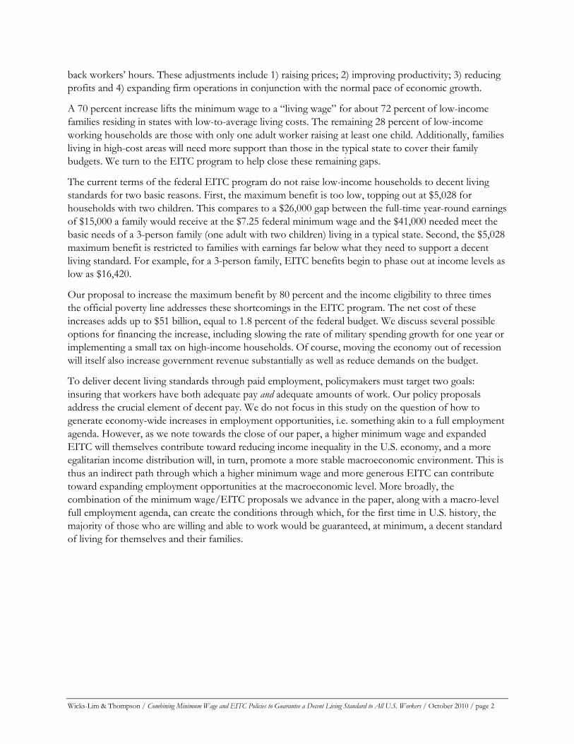
Most minimum wage rates do not adjust automatically with inflation to maintain their purchasing power. By 2010, only eight states have adopted such adjustments.9 As a consequence, for most areas in the United States, the purchasing power of the effective minimum wage rate has fluctuated over time. In figure 1, we present the real value (in 2009 dollars) of the federal minimum since 1960 through 2009. The federal minimum reached its peak value in 1968, at $9.86 expressed in 2009 dollars, about 37 percent higher than where it stands today.
FIGURE 1: REAL VALUE OF THE FEDERAL MINIMUM WAGE FROM 1960 TO 2009
Source: Bureau of Labor Statistics, U.S. Department of Labor
7 These minimum wage laws cover most, but not all, workers. The Fair Labor Standards Act requires a federal minimum wage for an estimated 72 percent of workers (U.S. Department of Labor, 2001). The 28 percent of the workforce that is exempt from the minimum wage law are primarily salaried executive, administrative, and professional employees and outside sales workers (workers making sales or obtaining orders away from employer's place of business). 8 The other two cities include Santa Fe and Albuquerque, New Mexico. 9 These states include Washington, Vermont, Oregon, Montana, Missouri, Florida, Colorado, and Arizona.
Wicks-Lim & Thompson / Combining Minimum Wage and EITC Policies to Guarantee a Decent Living Standard to All U.S. Workers / October 2010 / page 8
Since the early 1980s, federal minimum wage increases have directly benefited about five percent of the U.S. workforce whose wages have risen in order to keep up with the federal minimum. However, a larger group of workers also see their wages rise even though their raises are not required by law. This is because employers commonly raise the pay rates of workers who earn rates just above the new minimum wage, not just of those workers whose wages must increase to meet the new minimum. Employers do this to preserve the wage hierarchy that existed prior to the minimum wage increase. This broader set of raises is referred to as “ripple-effect” raises. Ripple-effect raises typically result in adding another five to ten percent of the workforce to the group of workers who gain from federal minimum wage hikes. Overall then, including those who receive mandated raises plus those benefitting from ripple-effect raises, increases in the federal minimum wage tend to impact about 10 to 15 percent of the workforce, or about 14 to 21 million workers.10
Earned Income Tax Credit
The federal Earned Income Tax Credit (EITC) is the largest government income-transfer program in the United States. In 2009, more than 24 million families received some EITC benefit. Total benefits, including reduced tax payments and refunded credits, added up to $51 billion. If we also add the EITC expenditures made by states through state programs, the total EITC figure rises to nearly $53 billion. This compares to $17 billion in Temporary Aid to Needy Families (TANF) benefits and $37 billion in Supplemental Nutrition Assistance Program food benefits (SNAP, formerly called Food Stamps). On the one hand, the EITC program clearly represents the federal government’s chief policy tool to reduce poverty. On the other hand, when considered against other tax breaks the size of the EITC program is modest. For example, the mortgage interest tax deduction on federal income taxes, available primarily for middle and upper-income households, was $471 billion in 2008.
The Earned Income Tax credit program basically converts a tax credit into a cash transfer when a household owes less in taxes than their EITC credit. When this occurs, the household receives the difference in a check from the federal government. Of the $51 billion in EITC credits, the federal government sent more than $44 billion to families in the form of EITC refund checks. The average EITC check sent to households was therefore $2,308 in 2009.11
THE BASIC STRUCTURE
EITC benefits are determined basically by two factors: the number of dependent children in the family and the total level of earnings from all working members in the family. The number of dependent children places households on one of three benefit schedules. On each schedule, the EITC benefit initially rises at a fixed rate along with earnings (the “phase-in” range) before hitting a maximum where the benefit stays constant as earnings rise (the “plateau” range). As earnings rise beyond the plateau range, the benefit is steadily reduced at a fixed rate until the total benefit is zero (the “phase-out” range).
10 Take for example, a recent estimate by the Economic Policy Institute (Mishel et al., 2008) of the federal minimum wage’s three-step raise from $5.15 to $7.25 that took place from 2007 to 2009. They estimate that 9.6 percent of the workforce in 2006 would see their wages rise due to such a change in the federal minimum. (p. 212). For estimates on the “ripple effect” of minimum wage hikes, see chapter 11 in Pollin et al. (2008). 11 These figures are provided by the Statistics of Income Division of the Internal Revenue Service. See: http://www.irs.gov/taxstats/article/0,,id=171535,00.html; accessed May 11, 2010..
Wicks-Lim & Thompson / Combining Minimum Wage and EITC Policies to Guarantee a Decent Living Standard to All U.S. Workers / October 2010 / page 9
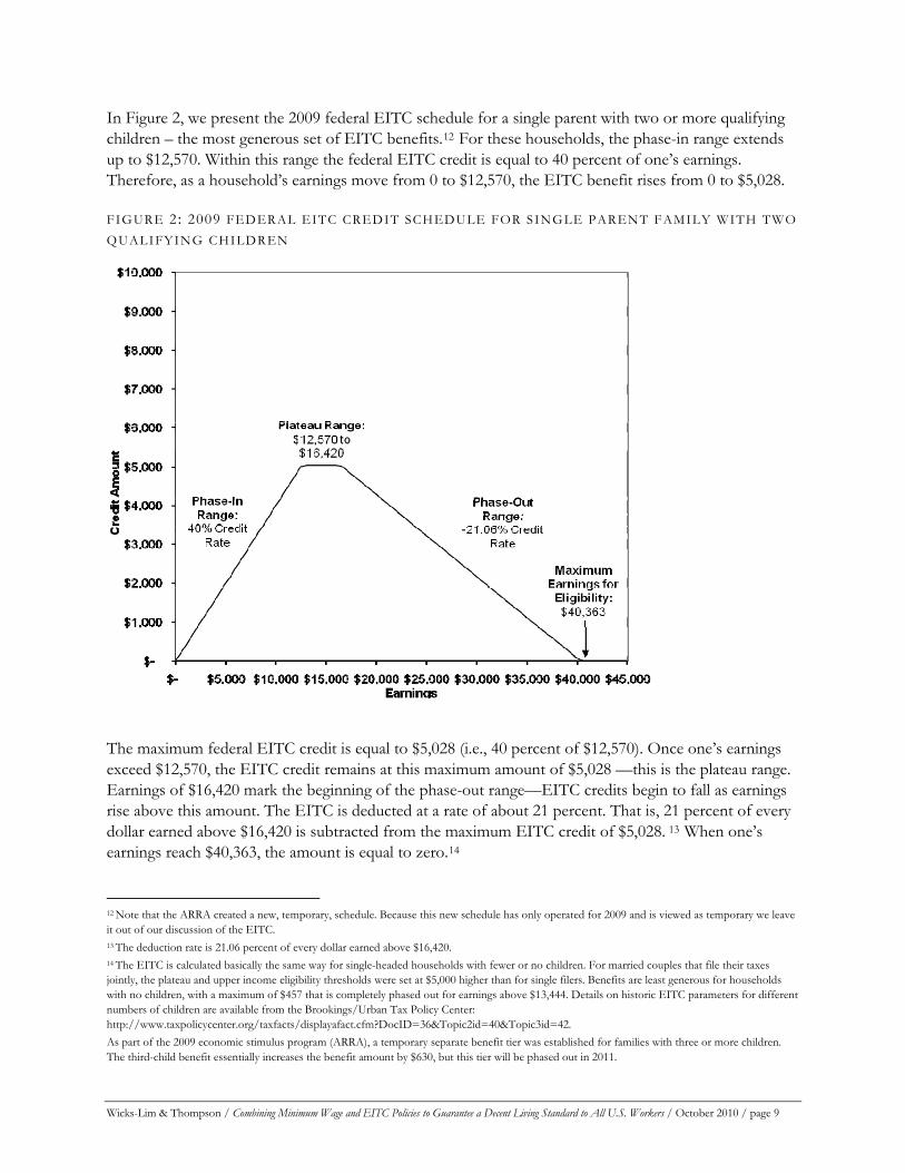
In Figure 2, we present the 2009 federal EITC schedule for a single parent with two or more qualifying children – the most generous set of EITC benefits.12 For these households, the phase-in range extends up to $12,570. Within this range the federal EITC credit is equal to 40 percent of one’s earnings. Therefore, as a household’s earnings move from 0 to $12,570, the EITC benefit rises from 0 to $5,028.
FIGURE 2: 2009 FEDERAL EITC CREDIT SCHEDULE FOR SINGLE PARENT FAMILY WITH TWO QUALIFYING CHILDREN
The maximum federal EITC credit is equal to $5,028 (i.e., 40 percent of $12,570). Once one’s earnings exceed $12,570, the EITC credit remains at this maximum amount of $5,028 —this is the plateau range. Earnings of $16,420 mark the beginning of the phase-out range—EITC credits begin to fall as earnings rise above this amount. The EITC is deducted at a rate of about 21 percent. That is, 21 percent of every dollar earned above $16,420 is subtracted from the maximum EITC credit of $5,028. 13 When one’s earnings reach $40,363, the amount is equal to zero.14
12 Note that the ARRA created a new, temporary, schedule. Because this new schedule has only operated for 2009 and is viewed as temporary we leave it out of our discussion of the EITC. 13 The deduction rate is 21.06 percent of every dollar earned above $16,420. 14 The EITC is calculated basically the same way for single-headed households with fewer or no children. For married couples that file their taxes jointly, the plateau and upper income eligibility thresholds were set at $5,000 higher than for single filers. Benefits are least generous for households with no children, with a maximum of $457 that is completely phased out for earnings above $13,444. Details on historic EITC parameters for different numbers of children are available from the Brookings/Urban Tax Policy Center: http://www.taxpolicycenter.org/taxfacts/displayafact.cfm?DocID=36&Topic2id=40&Topic3id=42. As part of the 2009 economic stimulus program (ARRA), a temporary separate benefit tier was established for families with three or more children. The third-child benefit essentially increases the benefit amount by $630, but this tier will be phased out in 2011.
Wicks-Lim & Thompson / Combining Minimum Wage and EITC Policies to Guarantee a Decent Living Standard to All U.S. Workers / October 2010 / page 10
This structure of EITC credits—with the phase-in, plateau, and phase-out ranges—shapes the work incentives that the program provides. The phase-in range provides the strongest incentive for work, effectively raising the total income people receive from work by 40 percent. Once we move into the plateau and phase-out ranges, the EITC credit can still provide a work incentive for those choosing between working and not working, but it does not provide any incentive for those already employed to work more. This is because the EITC credit no longer increases with additional earnings in this range. The phase-out range may actually provide a work disincentive, since a worker’s EITC credit is reduced for each additional dollar earned.
STATE ADD-ONS TO THE EITC
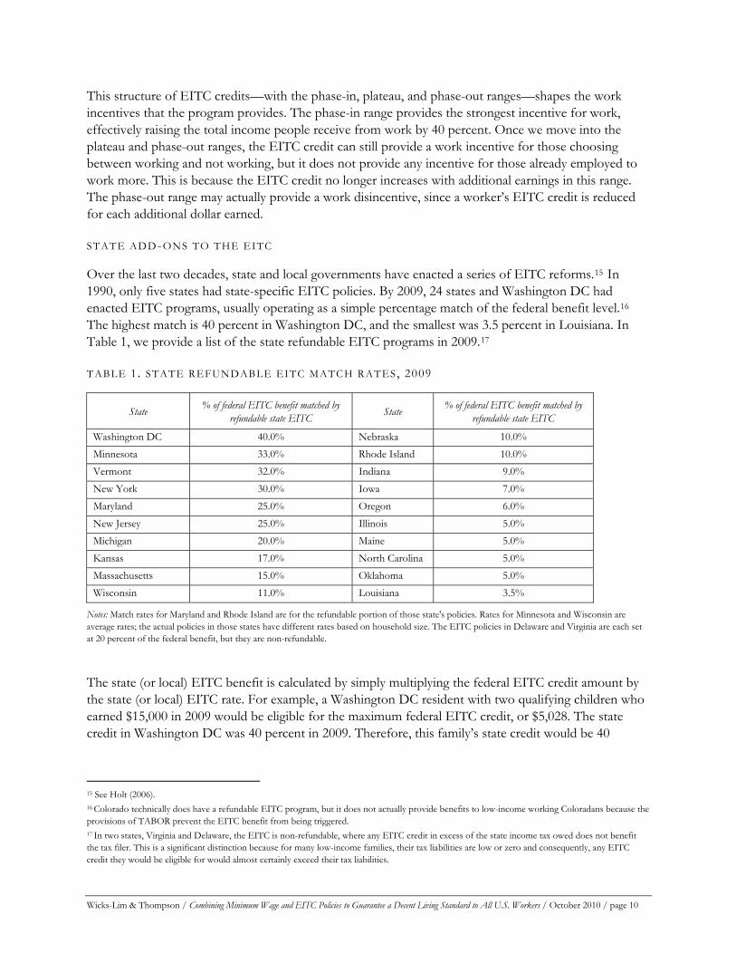
Over the last two decades, state and local governments have enacted a series of EITC reforms.15 In 1990, only five states had state-specific EITC policies. By 2009, 24 states and Washington DC had enacted EITC programs, usually operating as a simple percentage match of the federal benefit level.16 The highest match is 40 percent in Washington DC, and the smallest was 3.5 percent in Louisiana. In Table 1, we provide a list of the state refundable EITC programs in 2009.17
TABLE 1. STATE REFUNDABLE EITC MATCH RATES, 2009
State % of federal EITC benefit matched by refundable state EITC State % of federal EITC benefit matched by
refundable state EITC
Washington DC 40.0% Nebraska 10.0% Minnesota 33.0% Rhode Island 10.0% Vermont 32.0% Indiana 9.0% New York 30.0% Iowa 7.0% Maryland 25.0% Oregon 6.0% New Jersey 25.0% Illinois 5.0% Michigan 20.0% Maine 5.0% Kansas 17.0% North Carolina 5.0% Massachusetts 15.0% Oklahoma 5.0% Wisconsin 11.0% Louisiana 3.5%
Notes: Match rates for Maryland and Rhode Island are for the refundable portion of those state's policies. Rates for Minnesota and Wisconsin are average rates; the actual policies in those states have different rates based on household size. The EITC policies in Delaware and Virginia are each set at 20 percent of the federal benefit, but they are non-refundable.
The state (or local) EITC benefit is calculated by simply multiplying the federal EITC credit amount by the state (or local) EITC rate. For example, a Washington DC resident with two qualifying children who earned $15,000 in 2009 would be eligible for the maximum federal EITC credit, or $5,028. The state credit in Washington DC was 40 percent in 2009. Therefore, this family’s state credit would be 40
15 See Holt (2006). 16 Colorado technically does have a refundable EITC program, but it does not actually provide benefits to low-income working Coloradans because the provisions of TABOR prevent the EITC benefit from being triggered. 17 In two states, Virginia and Delaware, the EITC is non-refundable, where any EITC credit in excess of the state income tax owed does not benefit the tax filer. This is a significant distinction because for many low-income families, their tax liabilities are low or zero and consequently, any EITC credit they would be eligible for would almost certainly exceed their tax liabilities.
Wicks-Lim & Thompson / Combining Minimum Wage and EITC Policies to Guarantee a Decent Living Standard to All U.S. Workers / October 2010 / page 11
percent of their federal credit of $5,028, or about $2,011.18 In total, this household would receive a refundable credit of $7,039.
Defining a Decent Standard of Living
There is no official definition of a decent living standard. Instead, the U.S. Census Bureau publishes an official poverty income threshold. This official poverty level, however, is well-known to be too low as a measure of actual poverty.19 In fact, one study found that nearly two-thirds of families with incomes between the official poverty line and twice the official poverty line experienced serious economic hardships such as worrying about having enough food, having utilities disconnected, or depending on the emergency room as a main source of medical care.20 Moreover, public subsidy programs, such as the Low Income Home Energy Assistance Program and the State Children’s Health Insurance Program, use twice the official poverty income threshold as their income eligibility cutoffs, implying that families with incomes below 200 percent of the official poverty threshold are in economic distress. Consequently, an income level above at least 200 percent of the official poverty line would seem to more adequately represent income sufficient to meet the basic needs of a family than the official poverty line.
An alternative to the official poverty line, the basic family budget, has been created by economists at the Economic Policy Institute and is described in the report, What We Need to Get By.21 These basic family budgets provide an estimate of the income which families with young children need for a safe and decent, yet basic, living standard. These family budgets improve on the official poverty income thresholds by using regionally specific cost estimates for basic items including food, shelter, clothing, transportation, taxes (liabilities and credits), health care, and childcare. These basic budgets do not include any extras for eating out, entertainment, or even savings for emergencies, retirement, or education.
The basic family budget ranges from just below twice the poverty line to more than three times the poverty line. This wide range primarily reflects how living costs vary considerably across the country. Take for example, the state of New York. The average basic budget income threshold in the state of New York is $62,882 for a family of three. This is more than 50 percent greater than $40,746, the average across all states. A large part of this difference reflects the high housing costs of New York City where 43 percent of New York state residents live.22 The budget amounts also vary by household structure, that is, the number of children and adults present. We use this basic budget income threshold as our decent living standard measure. We refer to families with incomes that fall below this threshold as low-income. 18 Only a handful of states diverge from this simple formula. These include: 1) Minnesota, which has an entirely independent policy not based on the federal government definitions and eligibility levels, 2) Wisconsin, which has different rates for different family types, 3) Michigan, which does not provide any state match to childless workers, but provides a separate matching rate depending on whether the family has one, two, or three or more children, and 4) Maryland and Rhode Island each have hybrid refundable/non-refundable policies, with separate matching rates for a refundable and a non-refundable credit. For details about these exceptions, see the publication “A Hand Up,” published in various years by the Center for Budget and Policy Priorities (e.g., Nagle and Johnson 2006). 19 Constance Citro and Robert Michael (1995) offer a comprehensive discussion of the problems with the U.S. government’s official poverty measures in Measuring Poverty (Washington DC: National Academy Press). More recently, the U.S. Census Bureau announced its plan to develop an alternative poverty measure to address problems documented in Measuring Poverty, as well in the research that has been produced during the intervening years. This effort is described in the March 2010 U.S. Census Bureau memo titled, “Observations from the Interagency Technical Working Group on Developing a Supplemental Poverty Measure.” (http://www.census.gov/hhes/www/poverty/SPM_TWGObservations.pdf ) 20 Boushey, Brocht, Gundersen, and Bernstein (2001, p.30). 21 Lin and Bernstein (2008). 22 U.S. Census Bureau.
Wicks-Lim & Thompson / Combining Minimum Wage and EITC Policies to Guarantee a Decent Living Standard to All U.S. Workers / October 2010 / page 12
Do Current Policies Guarantee Families a Decent Living Standard Through Paid Employment?
The EITC and minimum wage policies underpinned the major shift in the federal government’s anti-poverty efforts during the mid-1990s to “make work pay.” To achieve this end, the Clinton administration pushed through a two-step federal minimum wage hike in 1996 and 1997 and at the same time, significantly expanded EITC benefits. These two combined policy expansions guaranteed that a full-time year-round job would pay enough income to support a small family of three at a living standard just above the official federal poverty line as defined by the U.S. Census Bureau.
The official poverty line, however, is insufficient to meet any reasonable definition of a decent living standard for the reasons we cited earlier. At no time in the history of the EITC policies and minimum wage laws have these policies operated at levels that achieve a decent, as opposed to impoverished, living standard.
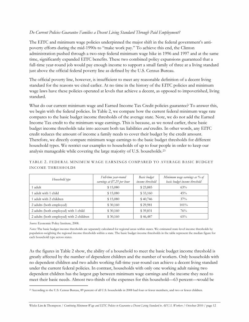
What do our current minimum wage and Earned Income Tax Credit policies guarantee? To answer this, we begin with the federal policies. In Table 2, we compare how the current federal minimum wage rate compares to the basic budget income thresholds of the average state. Note, we do not add the Earned Income Tax credit to the minimum wage earnings. This is because, as we noted earlier, these basic budget income thresholds take into account both tax liabilities and credits. In other words, any EITC credit reduces the amount of income a family needs to cover their budget by the credit amount. Therefore, we directly compare minimum wage earnings to the basic budget thresholds for different household types. We restrict our examples to households of up to four people in order to keep our analysis manageable while covering the large majority of U.S. households.23
TABLE 2. FEDERAL MINIMUM WAGE EARNINGS COMPARED TO AVERAGE BASIC BUDGET INCOME THRESHOLDS
Household type Full-time year-round earnings at $7.25 per hour
Basic budget income threshold
Minimum wage earnings as % of basic budget income threshold
1 adult $ 15,080 $ 23,885 63% 1 adult with 1 child $ 15,080 $ 33,160 45% 1 adult with 2 children $ 15,080 $ 40,746 37% 2 adults (both employed) $ 30,160 $ 29,981 101% 2 adults (both employed) with 1 child $ 30,160 $ 39,831 76% 2 adults (both employed) with 2 children $ 30,160 $ 46,487 65%
Source: Economic Policy Institute, 2008.
Notes: The basic budget income thresholds are separately calculated for regional areas within states. We estimated state-level income thresholds by population-weighting the regional income thresholds within a state. The basic budget income thresholds in the table represent the median figure for each household type across states.
As the figures in Table 2 show, the ability of a household to meet the basic budget income threshold is greatly affected by the number of dependent children and the number of workers. Only households with no dependent children and two adults working full-time year-round can achieve a decent living standard under the current federal policies. In contrast, households with only one working adult raising two dependent children has the largest gap between minimum wage earnings and the income they need to meet their basic needs. Almost two-thirds of the expenses for this household—63 percent—would be 23 According to the U.S. Census Bureau, 89 percent of all U.S. households in 2008 had four or fewer members, and two or fewer children.
left unmet by a minimum wage job. Clearly, this type of household faces the biggest challenge in achieving a decent living standard. Even in households that have two adults working, if they have dependent children, the federal minimum wage still leaves about one-quarter to one-third of their families’ basic needs unmet.
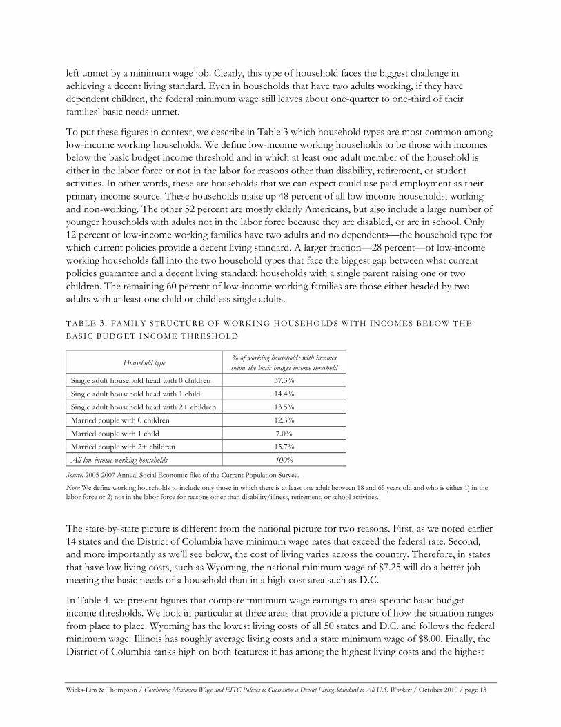
To put these figures in context, we describe in Table 3 which household types are most common among low-income working households. We define low-income working households to be those with incomes below the basic budget income threshold and in which at least one adult member of the household is either in the labor force or not in the labor for reasons other than disability, retirement, or student activities. In other words, these are households that we can expect could use paid employment as their primary income source. These households make up 48 percent of all low-income households, working and non-working. The other 52 percent are mostly elderly Americans, but also include a large number of younger households with adults not in the labor force because they are disabled, or are in school. Only 12 percent of low-income working families have two adults and no dependents—the household type for which current policies provide a decent living standard. A larger fraction—28 percent—of low-income working households fall into the two household types that face the biggest gap between what current policies guarantee and a decent living standard: households with a single parent raising one or two children. The remaining 60 percent of low-income working families are those either headed by two adults with at least one child or childless single adults.
TABLE 3. FAMILY STRUCTURE OF WORKING HOUSEHOLDS WITH INCOMES BELOW THE BASIC BUDGET INCOME THRESHOLD
Household type % of working households with incomes below the basic budget income threshold
Single adult household head with 0 children 37.3% Single adult household head with 1 child 14.4% Single adult household head with 2+ children 13.5% Married couple with 0 children 12.3% Married couple with 1 child 7.0% Married couple with 2+ children 15.7% All low-income working households 100%
Source: 2005-2007 Annual Social Economic files of the Current Population Survey.
Note: We define working households to include only those in which there is at least one adult between 18 and 65 years old and who is either 1) in the labor force or 2) not in the labor force for reasons other than disability/illness, retirement, or school activities.
The state-by-state picture is different from the national picture for two reasons. First, as we noted earlier 14 states and the District of Columbia have minimum wage rates that exceed the federal rate. Second, and more importantly as we’ll see below, the cost of living varies across the country. Therefore, in states that have low living costs, such as Wyoming, the national minimum wage of $7.25 will do a better job meeting the basic needs of a household than in a high-cost area such as D.C.
In Table 4, we present figures that compare minimum wage earnings to area-specific basic budget income thresholds. We look in particular at three areas that provide a picture of how the situation ranges from place to place. Wyoming has the lowest living costs of all 50 states and D.C. and follows the federal minimum wage. Illinois has roughly average living costs and a state minimum wage of $8.00. Finally, the District of Columbia ranks high on both features: it has among the highest living costs and the highest
Wicks-Lim & Thompson / Combining Minimum Wage and EITC Policies to Guarantee a Decent Living Standard to All U.S. Workers / October 2010 / page 13

Wicks-Lim & Thompson / Combining Minimum Wage and EITC Policies to Guarantee a Decent Living Standard to All U.S. Workers / October 2010 / page 14
minimum wage rate of $8.25.24 We focus our attention on the situation of 1 adult/2 child households since they have the greatest gap between minimum wage earnings and their basic budget income threshold. If a state’s current policies narrow the gap for this household type, then we can be assured that the gap is smaller still for other household types.
TABLE 4. STATE MINIMUM WAGE EARNINGS COMPARED TO THE BASIC BUDGET INCOME THRESHOLD FOR A FAMILY OF 3 (1 ADULT, 2 CHILDREN) IN THREE REPRESENTATIVE AREAS
Area Current minimum wage
Full-time year-round minimum wage earnings
Basic budget income threshold for a family of three (1 adult/2 children)
% of basic budget covered by minimum wage earnings
Wyoming $ 7.25 $ 15,080 $ 30,453 49.5% Illinois $ 8.00 $ 16,640 $ 43, 351 38.4% District of Columbia $ 8.25 $ 17,160 $ 65,631 26.1%
Source: Economic Policy Institute (2008). State-by-state figures are available upon request from authors.
In the 2nd column we show the annual earnings for a full-time year-round minimum wage job. Next to these earnings, we provide the states’ average basic budget income threshold—our decent living income standard—for a family of three (one adult, two children). In the 4th column we show what percentage of the basic family budget would be covered by the minimum wage earnings.
Across the 50 states and the District of Columbia, this small family with a full-time year-round minimum wage worker fares best in Wyoming. From the figures in the last two columns we can see that the living costs in Wyoming are low enough that the $7.25 minimum rate could support almost half of a small family’s budget. A small family in Illinois, because of higher living costs, cannot cover as much of their basic budget (38 percent) even with a higher minimum wage. The situation is among the worst for a family in the high-cost area of D.C. Its high minimum wage of $8.25 would cover just over one-quarter of a family’s basic budget.
The situations in these three areas represent the range of situations facing families across the 50 states and D.C. Current policies clearly fall far short of the policy goal to “make work pay.”
24 A listing of state-by-state figures (including figures for D.C.) is available from the authors up request.
Wicks-Lim & Thompson / Combining Minimum Wage and EITC Policies to Guarantee a Decent Living Standard to All U.S. Workers / October 2010 / page 15
CAN A MINIMUM WAGE BE A LIVING WAGE?
We know from past experience that the U.S. economy has supported a much higher federal minimum wage rate than where it is currently set at $7.25. From 1960 to 2009, the federal minimum has ranged from a low of $5.48 in 2006 to its peak value of $9.86 in 1968 (2009 dollars). We have also just seen in the previous section, however, that minimum wage rates would need rise even higher than this peak value to support a decent living standard. What we do not know is how high we could raise minimum wage rates without experiencing a significant decline in employment. There is no research that we are aware of that identifies a minimum wage “tipping point”—the largest minimum wage increase that firms can adjust to before turning to layoffs, or cutting back work schedules.
In this section, we use past research findings to develop a method that can identify the minimum wage tipping point. Specifically, we bring observations on how much minimum wage hikes cause business costs to rise together with industry research on how firms can adjust to such cost increases before turning to layoffs or cutting back on workers’ hours. By doing so, we can establish an upper limit to how large of a minimum wage hike can be before producing negative employment effects. In determining the highest minimum wage we can expect firms to absorb, we are able to evaluate whether minimum wage rates can rise up to living wage levels.
The overall body of empirical evidence suggests that past minimum wage and living wage increases have not lead to significant job losses. In fact, Doucouliagos and Stanley (2007) concluded, after analyzing over 64 separate studies on this question published between 1970 and 2007 that there is “little or no evidence of a negative association between minimum wages and employment...”25 Their conclusion is consistent with Harvard economist Richard Freeman’s assessment of the state of knowledge on this question 15 years earlier, “The debate is over whether modest minimum wage increases have ‘no’ employment effect, modest positive effects, or small negative effects. It is not about whether or not there are large negative effects (Freeman, 1995, p. 833).”
If, however, minimum wage and living wage laws lead to higher wages among low wage workers and increase employers’ wage bills, why isn’t there any notable employment loss? The basic economic theory of demand would suggest that when the price of something goes up, in this case, the price of labor, demand for that labor should fall, assuming all other aspects of the economy stay the same.
Two basic factors that have been observed in past research can explain the absence of any significant employment loss resulting from a minimum wage hike. First, the costs of these minimum wage hikes are small relative to the capacity of businesses to absorb them. As a result, they have required only modest adjustments by the firms that must raise the wages of their workforce. Second, businesses are never faced with the situation where their wage bill rises and all other aspects of the economy remain the same. Instead, minimum wage hikes take place in a changing economic environment and some of these changes can help firms adjust to their higher wage bills. For example, higher wages can raise worker morale and productivity that, in turn, can offset some of the cost of the raises. We will consider such changes in the economic environment in more detail below.
25 This meta-analysis includes studies that estimate both the immediate impact of minimum wages on employment as well as a lagged impact which could result if employers of low-wage workers a) become reluctant to hire more workers after a minimum wage hike because of their higher labor costs, or b) employers adjust to minimum wage hikes slowly.
What are the business costs of minimum wage increases?
We take advantage of the empirical evidence produced by a cluster of studies of various past minimum wage hikes to answer this question. These studies, to which one of us has contributed (e.g., in Pollin et al., 2008), directly measure how much firms’ costs would rise, by industry, in response to a minimum wage hike. Specifically, each study calculates a “cost increase/sales” ratio. This ratio is an estimate of the overall cost increases associated with a minimum wage hike taken as a percentage of overall sales revenue. This ratio provides a gauge of how big or small the cost increases are relative to the capacity of firms to cover these costs. A straightforward way to think of this ratio is how much a firm would need to raise prices in order to generate enough new sales revenue to cover the cost increase associated with a higher minimum wage.
We present estimates of these cost increase/sales ratios from a sampling of these studies in Table 5. Take for example, the figures in Panel A taken from an economic analysis of the 2004 Florida ballot initiative to establish a state minimum wage one dollar above the $5.15 federal minimum wage in effect at the time—a 19 percent increase. In the first row, we see that the cost increase/sales ratio is 0.04 percent for businesses across all industries.
What does this figure of 0.04 percent represent? Let’s consider the cost increases first. There are three main components of this cost increase. First, there is the cost of the raises required by the new, higher minimum wage. This is the sum of the raises required to bring workers earning below the new minimum wage up to the new minimum, assuming work schedules remain the same. Added to these mandated raises is the cost of ripple-effect raises. This is the sum of the raises for workers whose wages would be lifted a bit above the new wage floor of $6.15, again assuming they will continue to work the same number of hours. The third source of the cost increase is the higher level of payroll taxes that employers will be responsible for given their increased payroll—this is equal to 7.65 percent of the minimum wage raises.
For the 2004 Florida $6.15 minimum wage proposal, the three cost increases totaled to $406 million. This total cost increase of $406 million from the new minimum wage would be shared among 470,000 private sector Florida firms that were operating in 2004. At the time of the study, Florida private sector firms brought in a total of $929 billion in annual sales revenue. Therefore, the estimated total cost increase for private firms in Florida due to the proposed minimum wage hike represents 0.04 percent of total sales revenue ($406 million/$929 billion). This 0.04 percent figure is the cost increase/sales ratio. In other words, the average Florida firm would have to raise its prices by 0.04 percent to generate enough sales revenue to fully cover the costs of the proposed 19 percent minimum wage hike. This is equivalent to a $100 purchase rising in price to $100.04.
The other cost increase/sales ratios presented in Table 5 are calculated the same way as described above but on an industry-by-industry basis. The cost increase/sales ratios vary quite a bit from industry to industry. Take for example, the restaurant industry. The cost increase/sales figure in the second row of Table 5 indicates that in order to cover the costs of the proposed Florida minimum wage increase, restaurants would need to raise their sales revenue by 0.69 percent. The figure is 1.32 percent for the part of the restaurant industry that is primarily made up of fast food restaurants, restaurants with a particularly high concentration of minimum wage workers. A cost increase of this size could be fully covered by raising fast food prices by 1.32 percent. A Big Mac, for example, would rise in price from $4.00 to $4.05. These cost figures are more than 17 times the average cost increase/sales ratio across all industries of 0.04 percent.
Wicks-Lim & Thompson / Combining Minimum Wage and EITC Policies to Guarantee a Decent Living Standard to All U.S. Workers / October 2010 / page 16
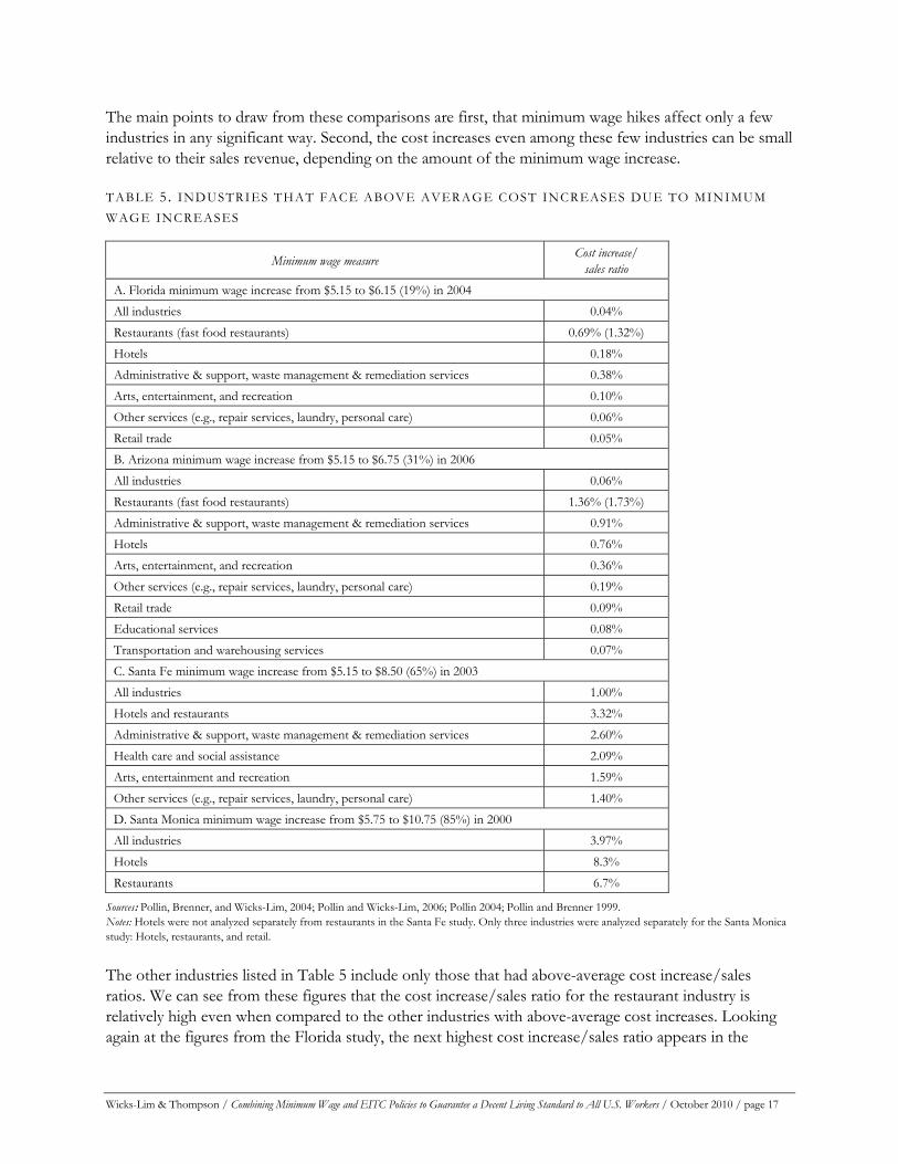
The main points to draw from these comparisons are first, that minimum wage hikes affect only a few industries in any significant way. Second, the cost increases even among these few industries can be small relative to their sales revenue, depending on the amount of the minimum wage increase.
TABLE 5. INDUSTRIES THAT FACE ABOVE AVERAGE COST INCREASES DUE TO MINIMUM WAGE INCREASES
Minimum wage measure Cost increase/ sales ratio
A. Florida minimum wage increase from $5.15 to $6.15 (19%) in 2004 All industries 0.04% Restaurants (fast food restaurants) 0.69% (1.32%) Hotels 0.18% Administrative & support, waste management & remediation services 0.38% Arts, entertainment, and recreation 0.10% Other services (e.g., repair services, laundry, personal care) 0.06% Retail trade 0.05% B. Arizona minimum wage increase from $5.15 to $6.75 (31%) in 2006 All industries 0.06% Restaurants (fast food restaurants) 1.36% (1.73%) Administrative & support, waste management & remediation services 0.91% Hotels 0.76% Arts, entertainment, and recreation 0.36% Other services (e.g., repair services, laundry, personal care) 0.19% Retail trade 0.09% Educational services 0.08% Transportation and warehousing services 0.07% C. Santa Fe minimum wage increase from $5.15 to $8.50 (65%) in 2003 All industries 1.00% Hotels and restaurants 3.32% Administrative & support, waste management & remediation services 2.60% Health care and social assistance 2.09% Arts, entertainment and recreation 1.59% Other services (e.g., repair services, laundry, personal care) 1.40% D. Santa Monica minimum wage increase from $5.75 to $10.75 (85%) in 2000 All industries 3.97% Hotels 8.3% Restaurants 6.7%
Sources: Pollin, Brenner, and Wicks-Lim, 2004; Pollin and Wicks-Lim, 2006; Pollin 2004; Pollin and Brenner 1999. Notes: Hotels were not analyzed separately from restaurants in the Santa Fe study. Only three industries were analyzed separately for the Santa Monica study: Hotels, restaurants, and retail.
The other industries listed in Table 5 include only those that had above-average cost increase/sales ratios. We can see from these figures that the cost increase/sales ratio for the restaurant industry is relatively high even when compared to the other industries with above-average cost increases. Looking again at the figures from the Florida study, the next highest cost increase/sales ratio appears in the
Wicks-Lim & Thompson / Combining Minimum Wage and EITC Policies to Guarantee a Decent Living Standard to All U.S. Workers / October 2010 / page 17

Wicks-Lim & Thompson / Combining Minimum Wage and EITC Policies to Guarantee a Decent Living Standard to All U.S. Workers / October 2010 / page 18
administrative and support and waste management and remediation services industry. This cost increase/sales ratio is only 0.38 percent, just over half the Florida restaurant industry’s 0.69 percent.
The figures in the Panel B of Table 5 are from a study of a 2006 Arizona proposal to raise the state minimum wage by 31 percent to $6.75. Panels C and D provide examples of minimum wage increases that are relatively large compared to most state minimum wage proposals: the Santa Fe citywide minimum enacted a 65 percent raise in their wage floor in 2004 and the area-wide $10.75 minimum wage for the Santa Monica coastal zone that passed in 2001 would have resulted in an 85 percent increase. This measure, however, was later eliminated by court order in 2002.26
For three out of the four studies, the industry facing the greatest cost increase relative to their sales revenue is the restaurant industry. Other industries that face above-average cost pressures from the proposed minimum wage hikes include: hotels; arts and entertainment; retail services; other services (e.g., repair, laundry, and private household services); health services; educational services; and transportation and warehousing services.
When we look at Panel D of Table 5, we see that the size of the proposed increase in the wage floor is significantly larger—85 percent, but the rise in the cost increase/sales ratios is still quite modest for the average business. The costs associated with the proposed 85 percent hike in the wage floor in Santa Monica would raise costs for the average firm across industries by only 1.0 percent of sales revenue. Again, restaurants would experience a noticeably higher cost increase of nearly seven percent of the sales revenue. Still, this suggests that a seven percent increase in restaurant prices could completely cover the costs of this area-wide minimum wage hike.
Why are business costs of minimum wage increases modest?
Three factors explain why minimum wage hikes tend to result in relatively small costs for businesses: 1) labor costs generally represent less than half of overall business costs, and frequently well below that; 2) for most industries, low-wage workers make up a small proportion of their workforce, and 3) many low-wage workers only receive a fraction of the actual size of a minimum wage hike because their current wages are already near what would be the new minimum rate.
First, a large share of a business’ costs is for things other than labor, such as machines, energy, and real estate. As a result, only a small proportion of sales revenue may be needed to cover payroll. In such cases, even a large increase in a company’s wage bill will amount to a small fraction of its total sales revenue. To illustrate, we provide, in Table 6, a comparison of the annual payroll in each industry to its total annual sales revenue. We present annual payroll figures by industry in the first column, total sales revenue by industry in the 2nd column, and payroll as a percentage of total sales in the last column. For the average industry, payroll is equal to about one-fifth (21 percent) of total sales, such as in the information services industry (e.g., publishing, broadcasting and telecommunication firms). Labor costs as a percentage of total sales are highest in the labor-intensive administrative and support services industry at 46 percent.
26 See Part 3 in Pollin et al. 2008 for a review of the outcome of the Santa Monica coastal zone ordinance.
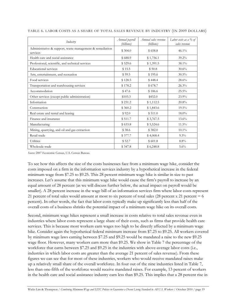
TABLE 6. LABOR COSTS AS A SHARE OF TOTAL SALES REVENUE BY INDUSTRY (IN 2009 DOLLARS)
Industry Annual payroll (billions)
Annual sales revenue (billions)
Labor costs as a % of sales revenue
Administrative & support, waste management & remediation services $ 304.0 $ 658.8 46.1%
Health care and social assistance $ 688.9 $ 1,756.1 39.2% Professional, scientific, and technical services $ 529.6 $ 1,391.5 38.1% Educational services $ 15.5 $ 50.8 30.6% Arts, entertainment, and recreation $ 59.5 $ 195.6 30.5% Food services $ 128.5 $ 448.4 28.6% Transportation and warehousing services $ 178.2 $ 678.7 26.3% Accommodation $ 47.6 $ 186.6 25.5% Other services (except public administration) $103.3 $432.0 23.9% Information $ 231.2 $ 1,112.5 20.8% Construction $ 360.2 $ 1,843.6 19.5% Real estate and rental and leasing $ 92.0 $ 511.0 18.0% Finance and insurance $ 511.7 $ 3,767.5 13.6% Manufacturing $ 633.8 $ 5,524.6 11.5% Mining, quarrying, and oil and gas extraction $ 38.6 $ 382.0 10.1% Retail trade $ 377.7 $ 4,068.4 9.3% Utilities $ 52.7 $ 601.8 8.8% Wholesale trade $ 347.8 $ 6,248.8 5.6%
Source: 2007 Economic Census, U.S. Census Bureau.
To see how this affects the size of the costs businesses face from a minimum wage hike, consider the costs imposed on a firm in the information services industry by a hypothetical increase in the federal minimum wage from $7.25 to $9.25. This 28 percent minimum wage hike is similar in size to past increases. Let’s assume that this minimum wage hike would cause the firm’s payroll to increase by an equal amount of 28 percent (as we will discuss further below, the actual impact on payroll would be smaller). A 28 percent increase in the wage bill of an information services firm where labor costs represent 21 percent of total sales would amount at most to six percent of total sales (28 percent x 21 percent = 6 percent). In other words, the fact that labor costs typically make up significantly less than half of the overall costs of a business shrinks the potential impact of a minimum wage hike on its overall costs.
Second, minimum wage hikes represent a small increase in costs relative to total sales revenue even in industries where labor costs represent a large share of their costs, such as firms that provide health care services. This is because most workers earn wages too high to be directly affected by a minimum wage hike. Consider again the hypothetical federal minimum increase from $7.25 to $9.25. All workers covered by minimum wage laws earning between $7.25 and $9.25 would be mandated a raise to the new $9.25 wage floor. However, many workers earn more than $9.25. We show in Table 7 the percentage of the workforce that earns between $7.25 and $9.25 in the industries with above-average labor costs (i.e., industries in which labor costs are greater than the average 21 percent of sales revenue). From these figures we can see that for most of these industries, workers who would receive mandated raises make up a relatively small share of the overall workforce. In four out of the nine industries listed in Table 7, less than one-fifth of the workforce would receive mandated raises. For example, 13 percent of workers in the health care and social assistance industry earn less than $9.25. This implies that a 28 percent rise in
Wicks-Lim & Thompson / Combining Minimum Wage and EITC Policies to Guarantee a Decent Living Standard to All U.S. Workers / October 2010 / page 19
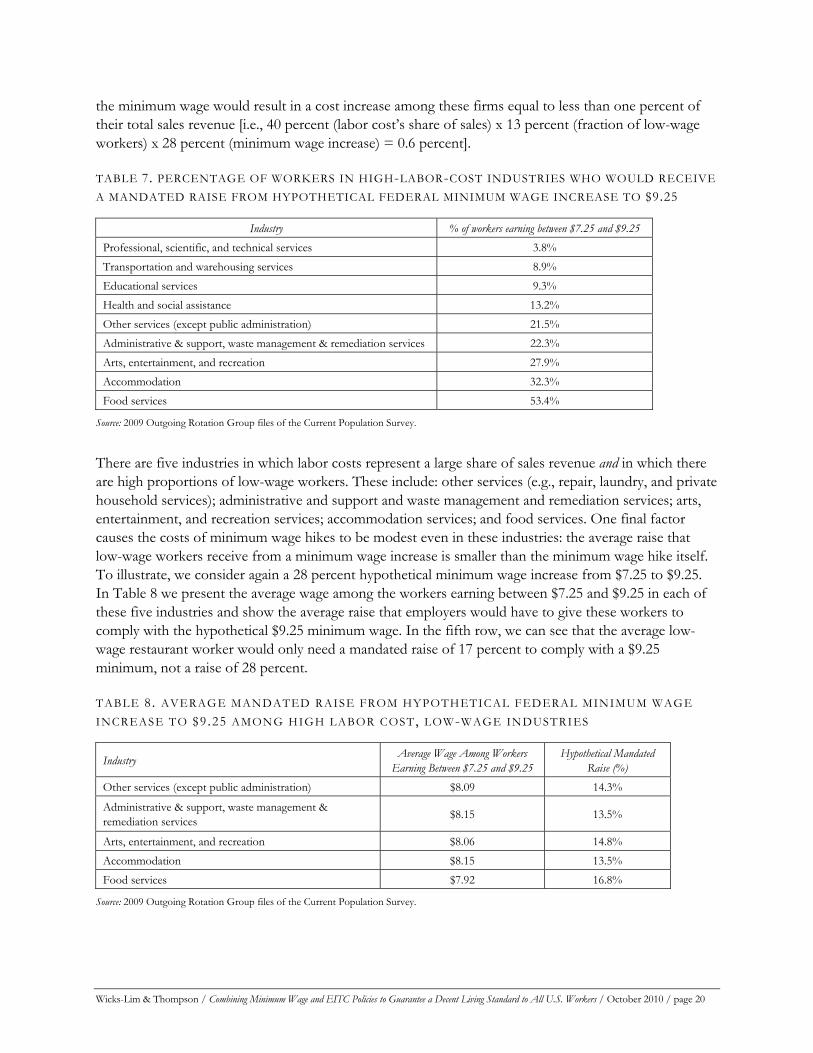
the minimum wage would result in a cost increase among these firms equal to less than one percent of their total sales revenue [i.e., 40 percent (labor cost’s share of sales) x 13 percent (fraction of low-wage workers) x 28 percent (minimum wage increase) = 0.6 percent].
TABLE 7. PERCENTAGE OF WORKERS IN HIGH-LABOR-COST INDUSTRIES WHO WOULD RECEIVE A MANDATED RAISE FROM HYPOTHETICAL FEDERAL MINIMUM WAGE INCREASE TO $9.25
Industry % of workers earning between $7.25 and $9.25 Professional, scientific, and technical services 3.8% Transportation and warehousing services 8.9% Educational services 9.3% Health and social assistance 13.2% Other services (except public administration) 21.5% Administrative & support, waste management & remediation services 22.3% Arts, entertainment, and recreation 27.9% Accommodation 32.3% Food services 53.4%
Source: 2009 Outgoing Rotation Group files of the Current Population Survey.
There are five industries in which labor costs represent a large share of sales revenue and in which there are high proportions of low-wage workers. These include: other services (e.g., repair, laundry, and private household services); administrative and support and waste management and remediation services; arts, entertainment, and recreation services; accommodation services; and food services. One final factor causes the costs of minimum wage hikes to be modest even in these industries: the average raise that low-wage workers receive from a minimum wage increase is smaller than the minimum wage hike itself. To illustrate, we consider again a 28 percent hypothetical minimum wage increase from $7.25 to $9.25. In Table 8 we present the average wage among the workers earning between $7.25 and $9.25 in each of these five industries and show the average raise that employers would have to give these workers to comply with the hypothetical $9.25 minimum wage. In the fifth row, we can see that the average low-wage restaurant worker would only need a mandated raise of 17 percent to comply with a $9.25 minimum, not a raise of 28 percent.
TABLE 8. AVERAGE MANDATED RAISE FROM HYPOTHETICAL FEDERAL MINIMUM WAGE INCREASE TO $9.25 AMONG HIGH LABOR COST, LOW-WAGE INDUSTRIES
Industry Average Wage Among Workers Earning Between $7.25 and $9.25
Hypothetical Mandated Raise (%)
Other services (except public administration) $8.09 14.3%
Administrative & support, waste management & remediation services $8.15 13.5%
Arts, entertainment, and recreation $8.06 14.8% Accommodation $8.15 13.5% Food services $7.92 16.8%
Source: 2009 Outgoing Rotation Group files of the Current Population Survey.
Wicks-Lim & Thompson / Combining Minimum Wage and EITC Policies to Guarantee a Decent Living Standard to All U.S. Workers / October 2010 / page 20
Wicks-Lim & Thompson / Combining Minimum Wage and EITC Policies to Guarantee a Decent Living Standard to All U.S. Workers / October 2010 / page 21
These three factors together reduce the impact of a 28 percent minimum wage increase on business costs even in the labor-intensive, low-wage restaurant industry to a relatively small fraction of sales revenue. Using the figures from Tables 6 to 8, we can roughly approximate a cost increase/sales ratio of three percent for restaurants [i.e., 29 percent (labor cost’s share of sales) x 53 percent (fraction of low-wage workers) x 17 percent (minimum wage increase) = 2.6 percent]. If we take into account that ripple effect raises and payroll taxes typically make up about 40 percent of the total cost increase firms face from a minimum wage hike, the restaurant industry’s cost increase/sales ratio rises to about four percent (2.6 percent/60 percent = 4.3 percent).27 And, in fact, this estimate falls within range of the 1 - 2 percent cost increase/sales ratio reported in the economic impact study by Pollin and Wicks-Lim for restaurants from a 31 percent increase in the Arizona minimum wage (see Panel B of Table 5).28
How can businesses adjust to these modest cost increases?
There are four basic ways for businesses to adjust to cost increases other than reducing employment. First, a minimum wage hike can be paid for, in part, by cost-savings from greater worker productivity and reduced turnover and training costs. Second, firms may pay for the higher wages by raising prices. Third, firms can use revenue increases from normal economic growth to cover a larger wage bill. Finally, firms can redistribute income within the firm—from profits to the wages of their lowest-paid workers or from high-wage workers to low-wage workers.
We focus on the most commonly observed ways that businesses adjust: greater worker productivity, higher prices, and growth. If businesses can adjust to a higher minimum wage through these channels, they will be able to do so without redistributing income within the firm. We assume that owners of firms, in their self-interest, will be most reluctant to reduce their profit rate. They may also be reluctant to reduce wages among high-wage workers because of the potential for such actions to damage worker morale. Therefore we do not figure these methods of adjustment into our calculations. Our estimate of how much firms can adjust to, therefore, is somewhat conservative. This is because whatever minimum wage hike we propose to be the tipping point, businesses should still have room to adjust a bit more.
Raising productivity. There is good reason to expect that firms will experience some labor-cost savings due to greater worker productivity. This is because minimum wage hikes can increase worker’s satisfaction and commitment to their job as their jobs give them access to higher income.29 One concrete way that these changes can be measured is through reduced turnover rates.30 With lower 27 Based on past studies (see Pollin et al. 2008), ripple effect raises typically make up 20 to 40 percent of the total cost increase, so we use the midpoint 30 percent to account for ripple effect raises. We add to this 7.65 percent in payroll taxes on new earnings to get about 40 percent. 28 The reason why our back-of-the-envelope estimate is somewhat higher than the Arizona study’s estimate is due to the following: The average size of the mandated raise and the fraction of workers expected to receive mandated raises that we projected would occur due to the Arizona proposal is smaller than what we assume for this exercise. This is because the Arizona measure appeared on the 2006 ballot, fully nine years after the last federal minimum wage hike in 1997. The wages of the lowest paid workers in Arizona likely rose somewhat above the federal minimum over those nine years. The figures we use in this exercise are based on 2009 wage data, the same year in which the federal minimum wage completed the third step of a three-step increase starting from $5.15 in 2007 to $7.25 by 2009. As a result, the lowest paid workers in 2009 are likely concentrated much closer to the federal minimum wage than was the case in Arizona in 2006. Therefore the same size minimum wage hike can be expected to affect a higher fraction of workers and require larger mandated raises in 2009 than was the case in Arizona in 2006. 29 Employers may also substitute workers in their current workforce with better-skilled workers after a minimum wage hike and thereby raise the productivity of their workforce. This assumes that the higher minimum wage allows employers to attract—or motivates employers to seek out—a pool of better-skilled workers. This would diminish the benefits to the intended beneficiaries of the minimum wage, currently employed low-wage workers. The empirical evidence on this suggests that some degree of substitution due to an increase in the wage floor does indeed occur but the large majority of the wage gains go to the intended beneficiaries (Fairris and Fernandez Bujanda, 2008). 30 For theoretical considerations of how higher wages may impact work effort see, for example, Akerlof and Yellen (1986), Bowles (1985) and Shapiro and Stiglitz (1985).

Wicks-Lim & Thompson / Combining Minimum Wage and EITC Policies to Guarantee a Decent Living Standard to All U.S. Workers / October 2010 / page 22
turnover, employers save on the costs of recruiting and training new employees and reap more benefits from the experience that employees gain over time. The cost saving that firms can achieve through lower turnover rates can help to offset the costs of a minimum wage hike.
This point immediately raises the following question: If businesses could raise the productivity of their workers and, as a result, save on labor costs, why don’t they do this regardless of any minimum wage hike? The answer is that the cost saving from productivity improvements induced by higher wages is unlikely to completely offset the cost of the higher wages. In other words, productivity improvements reduce, but do not completely eliminate, the cost of higher wages.
Raising prices. Firms can raise prices to generate more sales revenue that they can then use to cover their higher labor costs. The crucial question here is: how much can a firm raise prices without losing business? The answer to this question depends on what economists call the “price elasticity of demand.” The price elasticity of demand is a measure of how much consumers change their buying behavior in response to a change in price. If consumers are sensitive to changes in prices, the demand in that market is considered “elastic.” If consumers of a product or service do not change their buying behavior even as prices change, the demand in that market is considered to be “inelastic.” Businesses that operate in markets where demand is inelastic have more flexibility to raise their prices since their customers are unlikely to change what they buy even when prices rise.
This point raises a question about firms’ price-setting behavior that echoes the question we raised about firms’ wage-setting behavior above: Why don’t firms that operate in markets where demand is inelastic raise prices regardless of whether there is a minimum wage hike? This is because it can be difficult for a single firm to pursue this strategy alone. If one firm, among several within an industry, raises its prices it risks losing customers to local competition. Therefore, even if a firm would like to raise its prices to take advantage of an inelastic market demand, it will be reluctant to do so unless other firms also raise their prices. What is more likely to occur with a state minimum wage hike is that all affected firms in an area will raise their prices at about the same time. In this case, no one firm is placed at a disadvantage relative to their competitors, and all firms are able to enjoy the benefits of charging a higher price. In other words, each individual firm faces what economists refer to as a “coordination problem.” In the absence of an area-wide policy change like a minimum wage hike, firms have a hard time coordinating price increases with their competitors.31
Relying on economic growth. The overall health of the economy in which businesses operate can be an important factor in how firms adjust to a rise in their labor costs. This is because firms’ revenues tend to grow along with the overall economy. As the economy grows, so too do households’ incomes and this in turn causes the demand for many goods and services to rise.32 As a result, firms may find that the demand for their products or services is unchanged even if they raise prices and their consumer base is typically price sensitive. That is, higher prices can generate the same or higher level of consumer demand in the context of a growing economy. This is why, for example, when the federal minimum wage rose in two steps during 1996-1997, the Wall Street Journal ran a front-page article titled, “Chicken Feed: Minimum Wage Is Up, But a Fast Food Chain Notices Little Impact.” The article describes the operations of a fast food restaurant which raised prices in the range of 5 percent to 20 percent around the same time as the minimum wage hike and heard “hardly a peep from customers.” The store’s sales and profits rose over the same period. In the context of this robust economy, fears about the negative 31 Indeed, explicit efforts to coordinate prices —“price collusion”— is illegal in the United States. 32 From 1984 to 2009, the change in real personal consumer expenditures and real Gross Domestic Product growth track each other nearly one-for-one (Bureau of Economic Analysis, http://www.bea.gov/national/index.htm; accessed March 19, 2010).
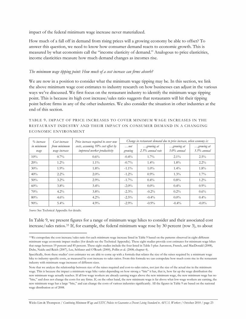
Wicks-Lim & Thompson / Combining Minimum Wage and EITC Policies to Guarantee a Decent Living Standard to All U.S. Workers / October 2010 / page 23
impact of the federal minimum wage increase never materialized.
How much of a fall off in demand from rising prices will a growing economy be able to offset? To answer this question, we need to know how consumer demand reacts to economic growth. This is measured by what economists call the “income elasticity of demand.” Analogous to price elasticities, income elasticities measure how much demand changes as incomes rise.
The minimum wage tipping point: How much of a cost increase can firms absorb?
We are now in a position to consider what the minimum wage tipping may be. In this section, we link the above minimum wage cost estimates to industry research on how businesses can adjust in the various ways we’ve discussed. We first focus on the restaurant industry to identify the minimum wage tipping point. This is because its high cost increase/sales ratio suggests that restaurants will hit their tipping point before firms in any of the other industries. We also consider the situation in other industries at the end of this section.
TABLE 9. IMPACT OF PRICE INCREASES TO COVER MINIMUM WAGE INCREASES IN THE RESTAURANT INDUSTRY AND THEIR IMPACT ON CONSUMER DEMAND IN A CHANGING ECONOMIC ENVIRONMENT
Change in restaurant demand due to price increase, when economy is: % increase in minimum
wage
Cost increase from minimum wage increase
Price increase required to cover new costs, assuming 10% cost offset by
improved worker productivity …not growing
…growing at 2.5% annual rate
…growing at 3.0% annual
…growing at 3.5% annual
10% 0.7% 0.6% -0.4% 1.7% 2.1% 2.5% 20% 1.2% 1.1% -0.7% 1.4% 1.8% 2.2% 30% 1.9% 1.8% -1.1% 1.0% 1.4% 1.8% 40% 2.2% 2.0% -1.2% 0.9% 1.3% 1.7% 50% 3.2% 2.9% -1.7% 0.4% 0.8% 1.2% 60% 3.8% 3.4% -2.0% 0.0% 0.4% 0.9% 70% 4.2% 3.8% -2.3% -0.2% 0.2% 0.6% 80% 4.6% 4.2% -2.5% -0.4% 0.0% 0.4% 90% 5.4% 4.9% -2.9% -0.9% -0.4% -0.0%
Source: See Technical Appendix for details.
In Table 9, we present figures for a range of minimum wage hikes to consider and their associated cost increase/sales ratios.33 If, for example, the federal minimum wage rose by 30 percent (row 3), to about 33 We extrapolate the cost increase/sales ratio for each minimum wage increase listed in Table 9 based on the patterns observed in eight different minimum wage economic impact studies (for details see the Technical Appendix). These eight studies provide cost estimates for minimum wage hikes that range between 19 percent and 85 percent. These eight studies include the four listed in Table 5 plus Aaronson, French, and MacDonald (2008), Dube, Naidu and Reich (2007), Lee, Schluter and O’Roark (2000), Pollin et al. (2008; chapter 4). Specifically, from these studies’ cost estimates we are able to come up with a formula that relates the size of the raises required by a minimum wage hike to industry-specific costs, as measured by cost increase-to-sales ratios. From this formula we can extrapolate how much costs rise in the restaurant industry with minimum wage increases of different sizes. Note that we analyze the relationship between size of the raises required and cost-to-sales ratios, not just the size of the actual rise in the minimum wage. This is because the impact a minimum wage hike varies depending on how strong a “bite” it has, that is, how far up the wage distribution the new minimum wage actually reaches. If all low-wage workers are already earning wages above the new minimum wage, the new minimum wage has no “bite,” and does not change the costs for any firms. If, on the other hand, the new minimum wage is far above what low-wage workers are earning, the new minimum wage has a large “bite,” and can change the costs of various industries significantly. All the figures in Table 9 are based on the national wage distribution as of 2008.

Wicks-Lim & Thompson / Combining Minimum Wage and EITC Policies to Guarantee a Decent Living Standard to All U.S. Workers / October 2010 / page 24
$9.40, the increased costs facing the restaurant industry would be equal to about 2 percent of sales revenue. This figure rises to 4 percent if the minimum wage rose by 70 percent to $12.30. We then illustrate in the remaining columns the extent to which the restaurant industry can absorb these cost increases in the various ways discussed above using the findings of industry research.
Productivity improvements. Three past studies provide estimates of cost savings that employers experience with an increase of a minimum wage or living wage. Take for example, a study by Fairris et al. (2005) that asked employers subject to the 1997 Los Angeles living wage ordinance about their turnover rate—the percentage of workers in their firm who quit or were fired over the course of one year. They estimate that the living wage ordinance reduced turnover rates by about 17 percentage points from 49 percent to 32 percent. After taking account of the costs to find and train new employees, this reduction in turnover rate produced cost savings equal to about 16 percent of the cost increase imposed by the living wage ordinance. The two other studies estimate such cost-savings in the range of 11 percent (San Francisco City Airport living wage ordinance; Reich, Hall and Jacobs, 2001) to 30 percent (Santa Fe citywide living wage ordinance; Pollin et al. 2008, ch. 5). Overall then, past studies suggest that this type of productivity increase may offset between 10 and 30 percent of the cost of a minimum wage hike. In column 3 of Table 9, we show the cost increase/sales ratio after accounting for a conservative 10 percent cost-savings estimate.
Price increases. We need to know how consumers are likely to react to price increases to determine how much restaurants could raise prices without losing any business activity. Raising prices without lowering consumer demand for their products and/or services would allow these businesses to generate the additional revenue they need to cover their increased costs. To gauge this, we compiled estimates of the price elasticity of demand for restaurant meals from two sources.
We first reviewed industry studies that estimate price elasticity of demand for restaurants.34 Two studies provide a range of -1.0 (Park et al. 1996) to -1.5 (Pigott 2003). Second, we conducted our own statistical analysis of consumer demand using the latest government data available (up to 2008) from the Department of Labor on household expenditures and the prices of restaurant meals to estimate a price elasticity of demand. Our estimate of -1.0 falls within the range of these other studies (see Technical Appendix for more information).
These price elasticities indicate how much, in percentage points, the demand for a product would rise or fall, if prices rise by 1 percent. Take, for example, our estimate of -1.0. This tells us that if restaurant prices rose by 1 percent, then demand for restaurant meals would fall by 1.0 percent. Price elasticities that are larger than one (whether positive or negative) are called “elastic” since such estimates indicate that the demand response is larger than the price change. Therefore, the demand for restaurant meals appears to be somewhat elastic.
There is good reason to question whether consumers would actually change their purchasing behavior in the face of the relatively small price changes that minimum wage hikes require. For example, a study of San Francisco’s 26 percent minimum wage hike found that after the rise in the wage floor the prices at fast food restaurants rose by six percent (Dube, Naidu, and Reich 2007). Despite this, employment levels stayed the same—in terms of number of jobs or hours of work. This implies that these price increases did not result in any notable decline in business activity. How can this be? 34 Note that the price elasticities we discuss are industry-wide measures. For example, the price elasticity of demand for restaurants is a measure of how consumer demand changes when all restaurants in an area change their prices not when an individual restaurant changes its prices while other nearby restaurants do not change their prices.
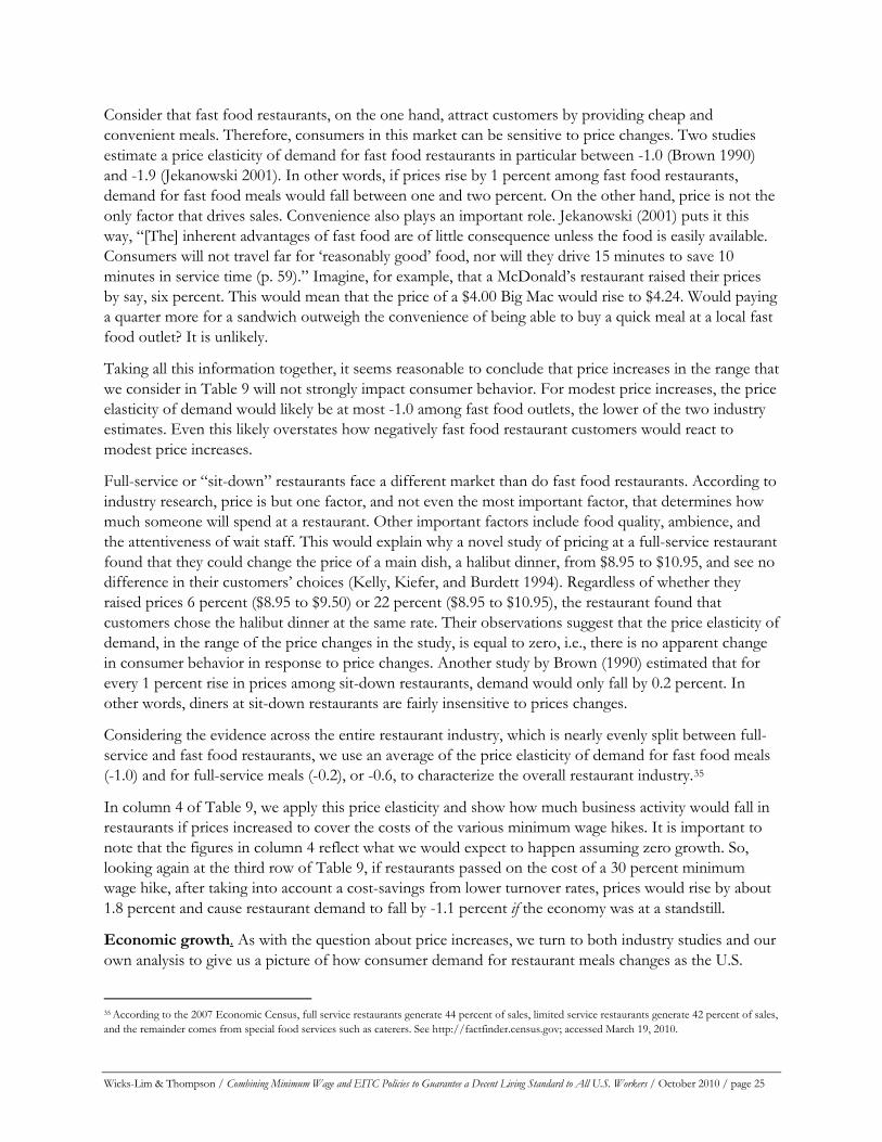
Wicks-Lim & Thompson / Combining Minimum Wage and EITC Policies to Guarantee a Decent Living Standard to All U.S. Workers / October 2010 / page 25
Consider that fast food restaurants, on the one hand, attract customers by providing cheap and convenient meals. Therefore, consumers in this market can be sensitive to price changes. Two studies estimate a price elasticity of demand for fast food restaurants in particular between -1.0 (Brown 1990) and -1.9 (Jekanowski 2001). In other words, if prices rise by 1 percent among fast food restaurants, demand for fast food meals would fall between one and two percent. On the other hand, price is not the only factor that drives sales. Convenience also plays an important role. Jekanowski (2001) puts it this way, “[The] inherent advantages of fast food are of little consequence unless the food is easily available. Consumers will not travel far for ‘reasonably good’ food, nor will they drive 15 minutes to save 10 minutes in service time (p. 59).” Imagine, for example, that a McDonald’s restaurant raised their prices by say, six percent. This would mean that the price of a $4.00 Big Mac would rise to $4.24. Would paying a quarter more for a sandwich outweigh the convenience of being able to buy a quick meal at a local fast food outlet? It is unlikely.
Taking all this information together, it seems reasonable to conclude that price increases in the range that we consider in Table 9 will not strongly impact consumer behavior. For modest price increases, the price elasticity of demand would likely be at most -1.0 among fast food outlets, the lower of the two industry estimates. Even this likely overstates how negatively fast food restaurant customers would react to modest price increases.
Full-service or “sit-down” restaurants face a different market than do fast food restaurants. According to industry research, price is but one factor, and not even the most important factor, that determines how much someone will spend at a restaurant. Other important factors include food quality, ambience, and the attentiveness of wait staff. This would explain why a novel study of pricing at a full-service restaurant found that they could change the price of a main dish, a halibut dinner, from $8.95 to $10.95, and see no difference in their customers’ choices (Kelly, Kiefer, and Burdett 1994). Regardless of whether they raised prices 6 percent ($8.95 to $9.50) or 22 percent ($8.95 to $10.95), the restaurant found that customers chose the halibut dinner at the same rate. Their observations suggest that the price elasticity of demand, in the range of the price changes in the study, is equal to zero, i.e., there is no apparent change in consumer behavior in response to price changes. Another study by Brown (1990) estimated that for every 1 percent rise in prices among sit-down restaurants, demand would only fall by 0.2 percent. In other words, diners at sit-down restaurants are fairly insensitive to prices changes.
Considering the evidence across the entire restaurant industry, which is nearly evenly split between full-service and fast food restaurants, we use an average of the price elasticity of demand for fast food meals (-1.0) and for full-service meals (-0.2), or -0.6, to characterize the overall restaurant industry.35
In column 4 of Table 9, we apply this price elasticity and show how much business activity would fall in restaurants if prices increased to cover the costs of the various minimum wage hikes. It is important to note that the figures in column 4 reflect what we would expect to happen assuming zero growth. So, looking again at the third row of Table 9, if restaurants passed on the cost of a 30 percent minimum wage hike, after taking into account a cost-savings from lower turnover rates, prices would rise by about 1.8 percent and cause restaurant demand to fall by -1.1 percent if the economy was at a standstill.
Economic growth. As with the question about price increases, we turn to both industry studies and our own analysis to give us a picture of how consumer demand for restaurant meals changes as the U.S.
35 According to the 2007 Economic Census, full service restaurants generate 44 percent of sales, limited service restaurants generate 42 percent of sales, and the remainder comes from special food services such as caterers. See http://factfinder.census.gov; accessed March 19, 2010.
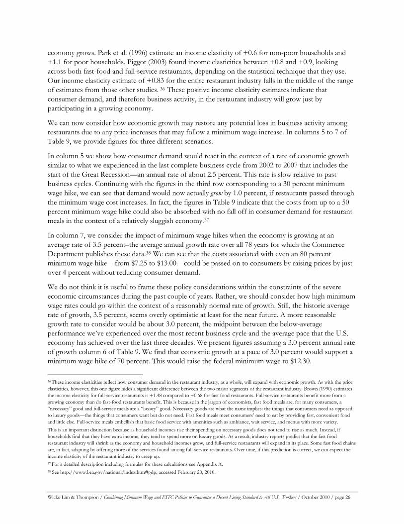
Wicks-Lim & Thompson / Combining Minimum Wage and EITC Policies to Guarantee a Decent Living Standard to All U.S. Workers / October 2010 / page 26
economy grows. Park et al. (1996) estimate an income elasticity of +0.6 for non-poor households and +1.1 for poor households. Piggot (2003) found income elasticities between +0.8 and +0.9, looking across both fast-food and full-service restaurants, depending on the statistical technique that they use. Our income elasticity estimate of +0.83 for the entire restaurant industry falls in the middle of the range of estimates from those other studies. 36 These positive income elasticity estimates indicate that consumer demand, and therefore business activity, in the restaurant industry will grow just by participating in a growing economy.
We can now consider how economic growth may restore any potential loss in business activity among restaurants due to any price increases that may follow a minimum wage increase. In columns 5 to 7 of Table 9, we provide figures for three different scenarios.
In column 5 we show how consumer demand would react in the context of a rate of economic growth similar to what we experienced in the last complete business cycle from 2002 to 2007 that includes the start of the Great Recession—an annual rate of about 2.5 percent. This rate is slow relative to past business cycles. Continuing with the figures in the third row corresponding to a 30 percent minimum wage hike, we can see that demand would now actually grow by 1.0 percent, if restaurants passed through the minimum wage cost increases. In fact, the figures in Table 9 indicate that the costs from up to a 50 percent minimum wage hike could also be absorbed with no fall off in consumer demand for restaurant meals in the context of a relatively sluggish economy.37
In column 7, we consider the impact of minimum wage hikes when the economy is growing at an average rate of 3.5 percent–the average annual growth rate over all 78 years for which the Commerce Department publishes these data.38 We can see that the costs associated with even an 80 percent minimum wage hike—from $7.25 to $13.00—could be passed on to consumers by raising prices by just over 4 percent without reducing consumer demand.
We do not think it is useful to frame these policy considerations within the constraints of the severe economic circumstances during the past couple of years. Rather, we should consider how high minimum wage rates could go within the context of a reasonably normal rate of growth. Still, the historic average rate of growth, 3.5 percent, seems overly optimistic at least for the near future. A more reasonable growth rate to consider would be about 3.0 percent, the midpoint between the below-average performance we’ve experienced over the most recent business cycle and the average pace that the U.S. economy has achieved over the last three decades. We present figures assuming a 3.0 percent annual rate of growth column 6 of Table 9. We find that economic growth at a pace of 3.0 percent would support a minimum wage hike of 70 percent. This would raise the federal minimum wage to $12.30.
36 These income elasticities reflect how consumer demand in the restaurant industry, as a whole, will expand with economic growth. As with the price elasticities, however, this one figure hides a significant difference between the two major segments of the restaurant industry. Brown (1990) estimates the income elasticity for full-service restaurants is +1.48 compared to +0.68 for fast food restaurants. Full-service restaurants benefit more from a growing economy than do fast-food restaurants benefit. This is because in the jargon of economists, fast food meals are, for many consumers, a “necessary” good and full-service meals are a “luxury” good. Necessary goods are what the name implies: the things that consumers need as opposed to luxury goods—the things that consumers want but do not need. Fast food meals meet consumers’ need to eat by providing fast, convenient food and little else. Full-service meals embellish that basic food service with amenities such as ambiance, wait service, and menus with more variety. This is an important distinction because as household incomes rise their spending on necessary goods does not tend to rise as much. Instead, if households find that they have extra income, they tend to spend more on luxury goods. As a result, industry reports predict that the fast food restaurant industry will shrink as the economy and household incomes grow, and full-service restaurants will expand in its place. Some fast food chains are, in fact, adapting by offering more of the services found among full-service restaurants. Over time, if this prediction is correct, we can expect the income elasticity of the restaurant industry to creep up. 37 For a detailed description including formulas for these calculations see Appendix A. 38 See http://www.bea.gov/national/index.htm#gdp; accessed February 20, 2010.

Wicks-Lim & Thompson / Combining Minimum Wage and EITC Policies to Guarantee a Decent Living Standard to All U.S. Workers / October 2010 / page 27
In practice, what this exercise implies is that the additional business activity that restaurants would gain in one year of low to average economic growth would be enough to make up for any potential loss in business activity from passing along the costs of a 70 percent minimum wage hike through to their customers in the form of higher prices. This means that the level of profits should remain the same since the additional revenue to cover the raises will be paid for by consumers who are willing to pay higher prices for the same level of goods and services. After this one year, business activity and profits should grow at the same pace as before with normal economic growth.
Other industries. We now turn back to the other industries we expect to experience above-average cost increases. We know that the cost increase/sale ratios for these other industries are smaller than the restaurant industry. Therefore, if consumers react similarly to price increases and economic growth in the markets of these other industries as in the restaurant industry, we would expect that these other industries would also be able to support a 70 percent increase in the minimum wage.
There are two reasons why this may not turn out to be the case. First, consumers may react more negatively to price increases in the products and services of these other industries. As a result, demand may fall at a faster rate for these other industries than in the restaurant industry. Second, consumers may not increase their spending on the products and services of these other industries at the same rate as in the restaurant industry as the economy grows. Therefore, economic growth may not restore as much of the fall off in consumer demand that may result from higher prices.
As before, we use industry studies to gauge the price and income elasticities of demand in these other markets. However, the estimates for both types of elasticities range quite a bit from study to study, and for some industries we could only find one or two estimates.39 Therefore, we can only make broad statements about the price and income elasticity of demand in these other industries.
The price elasticities of these other eight industries appear to be about the same or larger than the price elasticity of restaurant demand. In other words, consumers appear to react at least as strongly to price increases for the products and services of these other eight industries, as compared to the restaurant industry. Take for example, the arts, entertainment, and recreation industry. The average price elasticity estimate for this industry of -0.9 would predict that a 4 percent price increase would lead to a 3.6 percent decline in consumer demand for such things as music concerts and amusement park activities. In other words, this price elasticity predicts that if a $25 entrance ticket to an amusement park rose to $25.90 fewer people would purchase tickets. As in the case of the restaurant industry, this seems to overstate the impact of the small price increases we are considering. In any case, past research suggests that the markets in some of these other industries are likely to be as, or more, sensitive to price increases than in the restaurant industry.
The income elasticity estimates for these other eight industries are about the same or larger than the income elasticity of restaurant demand. That is, economic growth increases consumer demand for the products and services in the eight other industries by the same amount or more than in the restaurant industry. This seems reasonable since these other industries provide services that people typically like to spend more money on as their income grows, such as hotels, health services, and retail shopping.
We can now apply what we know about the price and income elasticities in these eight other industries to assess the impact of a 70 percent minimum wage hike. We repeat the same basic exercise for these eight industries that we did for the restaurant industry and present the relevant figures in Table 10. This 39 We provide a full list of these elasticities in the Technical Appendix.

Wicks-Lim & Thompson / Combining Minimum Wage and EITC Policies to Guarantee a Decent Living Standard to All U.S. Workers / October 2010 / page 28
time, however, we only consider a 70 percent minimum wage hike. For reference, we provide the figures for the restaurant industry in the first row of Table 10.
TABLE 10. IMPACT OF PRICE INCREASE TO COVER 70% MINIMUM WAGE ON CONSUMER DEMAND IN A CHANGING ECONOMIC ENVIRONMENT
Change in demand due to price increase, when economy is:
Industry
Cost increase from 70%
minimum wage hike
Price increase required to cover new costs, assuming 10% cost
offset by improved worker productivity …not growing …growing at 3.0%
annual rate Restaurants 4.2% 3.8% -2.3% 0.2% Hotels 4.8% 4.3% -1.7% 1.9% Administrative & support, waste management & remediation services 3.3% 3.0% -3.9% -0.6%
Health services 2.4% 2.2% -2.2% 0.2% Arts, entertainment and recreation 1.8% 1.6% -1.5% 3.0%
Other services (e.g., repair, laundry, and private household services) 1.6% 1.4% -1.2% 1.8%
Retail trade 0.9% 0.8% -0.7% 1.7% Educational services 0.4% 0.4% -0.2% 2.8% Transportation and warehousing services 0.8% 0.7% -0.7% 1.3%
Sources: See Technical Appendix.
In the second column of Table 10, we start with the cost increase/sale ratios for each industry that would result from a 70 percent minimum wage hike. As we already noted before, the cost increase/sales ratio for these industries are lower than that in the restaurant industry except for in the hotel industry. When the minimum wage hike is substantial the cost increase/sales ratio for the hotel industry rises to just above that in the restaurant industry.40
In the next column, we show how much of a price increase firms in each industry may pass on to consumers to cover the costs of the minimum wage increase, assuming that reductions in turnover would offset 10 percent of the cost increase. In the fourth column, we show how demand would be affected by the price increase alone, i.e., while the economy is at a standstill. The final column shows how business activity would change, assuming now a year of growth at an annual rate of 3.0 percent. What we can see from this final column is that firms in these other industries most likely have a greater ability, or at least as great an ability, to adjust to a 70 percent minimum wage hike.
The industry of administrative and support services is the one exception. Firms in this industry may see a slight decline in their business activity if they pass on their cost increase (net of the savings from productivity increases) to consumers of their services. This is because consumers of these services are relatively sensitive to price changes with a price elasticity of demand of -1.3. For this industry, firms may need to absorb a small amount of the cost increase, equal to -0.6 percent of sales revenue, in other ways. As we mentioned earlier, they may also redistribute income within the firm, i.e., from the salaries of higher wage workers to low-wage workers or the profits of firm owners to low-wage workers.
Overall, we conclude that a 70 percent minimum wage increase could be accommodated by all of these
40 This suggests that low-wage hotel workers are concentrated at wage rates near the minimum, but slightly higher than low-wage restaurant workers.
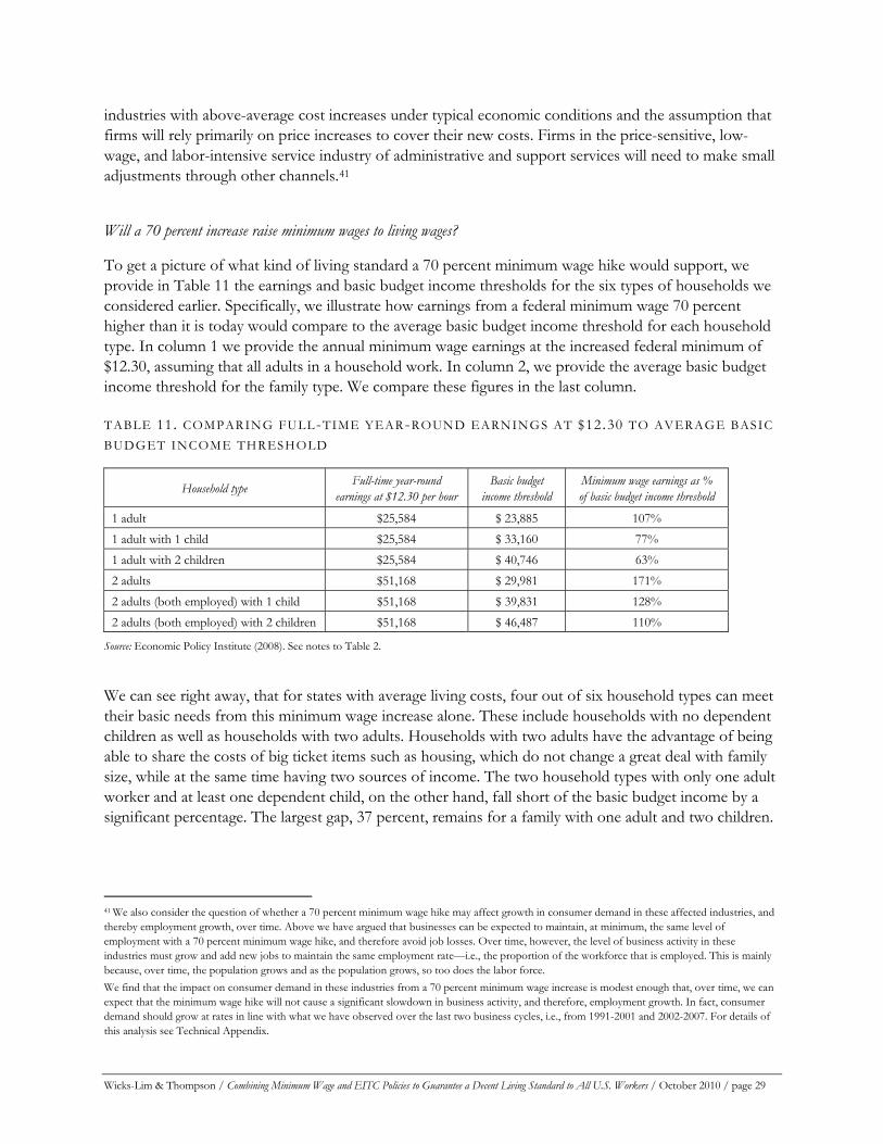
Wicks-Lim & Thompson / Combining Minimum Wage and EITC Policies to Guarantee a Decent Living Standard to All U.S. Workers / October 2010 / page 29
industries with above-average cost increases under typical economic conditions and the assumption that firms will rely primarily on price increases to cover their new costs. Firms in the price-sensitive, low-wage, and labor-intensive service industry of administrative and support services will need to make small adjustments through other channels.41
Will a 70 percent increase raise minimum wages to living wages?
To get a picture of what kind of living standard a 70 percent minimum wage hike would support, we provide in Table 11 the earnings and basic budget income thresholds for the six types of households we considered earlier. Specifically, we illustrate how earnings from a federal minimum wage 70 percent higher than it is today would compare to the average basic budget income threshold for each household type. In column 1 we provide the annual minimum wage earnings at the increased federal minimum of $12.30, assuming that all adults in a household work. In column 2, we provide the average basic budget income threshold for the family type. We compare these figures in the last column.
TABLE 11. COMPARING FULL-TIME YEAR-ROUND EARNINGS AT $12.30 TO AVERAGE BASIC BUDGET INCOME THRESHOLD
Household type Full-time year-round earnings at $12.30 per hour
Basic budget income threshold
Minimum wage earnings as % of basic budget income threshold
1 adult $25,584 $ 23,885 107% 1 adult with 1 child $25,584 $ 33,160 77% 1 adult with 2 children $25,584 $ 40,746 63% 2 adults $51,168 $ 29,981 171% 2 adults (both employed) with 1 child $51,168 $ 39,831 128% 2 adults (both employed) with 2 children $51,168 $ 46,487 110%
Source: Economic Policy Institute (2008). See notes to Table 2.
We can see right away, that for states with average living costs, four out of six household types can meet their basic needs from this minimum wage increase alone. These include households with no dependent children as well as households with two adults. Households with two adults have the advantage of being able to share the costs of big ticket items such as housing, which do not change a great deal with family size, while at the same time having two sources of income. The two household types with only one adult worker and at least one dependent child, on the other hand, fall short of the basic budget income by a significant percentage. The largest gap, 37 percent, remains for a family with one adult and two children.
41 We also consider the question of whether a 70 percent minimum wage hike may affect growth in consumer demand in these affected industries, and thereby employment growth, over time. Above we have argued that businesses can be expected to maintain, at minimum, the same level of employment with a 70 percent minimum wage hike, and therefore avoid job losses. Over time, however, the level of business activity in these industries must grow and add new jobs to maintain the same employment rate—i.e., the proportion of the workforce that is employed. This is mainly because, over time, the population grows and as the population grows, so too does the labor force. We find that the impact on consumer demand in these industries from a 70 percent minimum wage increase is modest enough that, over time, we can expect that the minimum wage hike will not cause a significant slowdown in business activity, and therefore, employment growth. In fact, consumer demand should grow at rates in line with what we have observed over the last two business cycles, i.e., from 1991-2001 and 2002-2007. For details of this analysis see Technical Appendix.
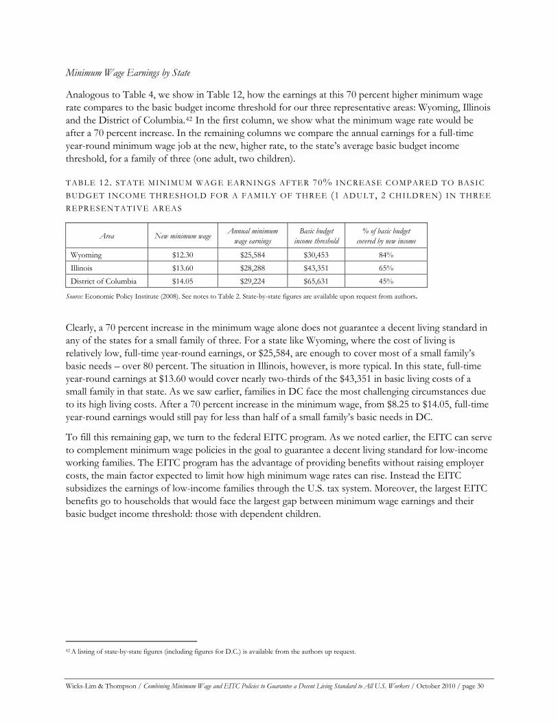
Wicks-Lim & Thompson / Combining Minimum Wage and EITC Policies to Guarantee a Decent Living Standard to All U.S. Workers / October 2010 / page 30
Minimum Wage Earnings by State
Analogous to Table 4, we show in Table 12, how the earnings at this 70 percent higher minimum wage rate compares to the basic budget income threshold for our three representative areas: Wyoming, Illinois and the District of Columbia.42 In the first column, we show what the minimum wage rate would be after a 70 percent increase. In the remaining columns we compare the annual earnings for a full-time year-round minimum wage job at the new, higher rate, to the state’s average basic budget income threshold, for a family of three (one adult, two children).
TABLE 12. STATE MINIMUM WAGE EARNINGS AFTER 70% INCREASE COMPARED TO BASIC BUDGET INCOME THRESHOLD FOR A FAMILY OF THREE (1 ADULT, 2 CHILDREN) IN THREE REPRESENTATIVE AREAS
Area New minimum wage Annual minimum wage earnings
Basic budget income threshold
% of basic budget covered by new income
Wyoming $12.30 $25,584 $30,453 84% Illinois $13.60 $28,288 $43,351 65% District of Columbia $14.05 $29,224 $65,631 45%
Source: Economic Policy Institute (2008). See notes to Table 2. State-by-state figures are available upon request from authors.
Clearly, a 70 percent increase in the minimum wage alone does not guarantee a decent living standard in any of the states for a small family of three. For a state like Wyoming, where the cost of living is relatively low, full-time year-round earnings, or $25,584, are enough to cover most of a small family’s basic needs – over 80 percent. The situation in Illinois, however, is more typical. In this state, full-time year-round earnings at $13.60 would cover nearly two-thirds of the $43,351 in basic living costs of a small family in that state. As we saw earlier, families in DC face the most challenging circumstances due to its high living costs. After a 70 percent increase in the minimum wage, from $8.25 to $14.05, full-time year-round earnings would still pay for less than half of a small family’s basic needs in DC.
To fill this remaining gap, we turn to the federal EITC program. As we noted earlier, the EITC can serve to complement minimum wage policies in the goal to guarantee a decent living standard for low-income working families. The EITC program has the advantage of providing benefits without raising employer costs, the main factor expected to limit how high minimum wage rates can rise. Instead the EITC subsidizes the earnings of low-income families through the U.S. tax system. Moreover, the largest EITC benefits go to households that would face the largest gap between minimum wage earnings and their basic budget income threshold: those with dependent children.
42 A listing of state-by-state figures (including figures for D.C.) is available from the authors up request.
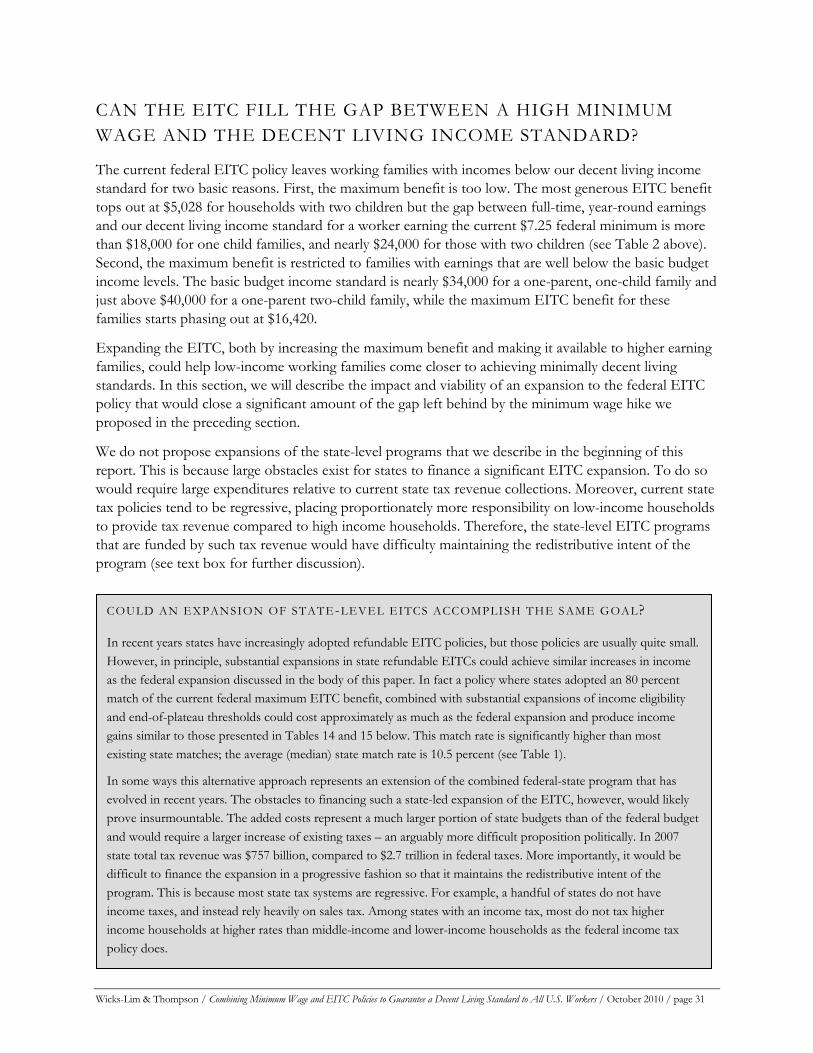
CAN THE EITC FILL THE GAP BETWEEN A HIGH MINIMUM WAGE AND THE DECENT LIVING INCOME STANDARD?
The current federal EITC policy leaves working families with incomes below our decent living income standard for two basic reasons. First, the maximum benefit is too low. The most generous EITC benefit tops out at $5,028 for households with two children but the gap between full-time, year-round earnings and our decent living income standard for a worker earning the current $7.25 federal minimum is more than $18,000 for one child families, and nearly $24,000 for those with two children (see Table 2 above). Second, the maximum benefit is restricted to families with earnings that are well below the basic budget income levels. The basic budget income standard is nearly $34,000 for a one-parent, one-child family and just above $40,000 for a one-parent two-child family, while the maximum EITC benefit for these families starts phasing out at $16,420.
Expanding the EITC, both by increasing the maximum benefit and making it available to higher earning families, could help low-income working families come closer to achieving minimally decent living standards. In this section, we will describe the impact and viability of an expansion to the federal EITC policy that would close a significant amount of the gap left behind by the minimum wage hike we proposed in the preceding section.
We do not propose expansions of the state-level programs that we describe in the beginning of this report. This is because large obstacles exist for states to finance a significant EITC expansion. To do so would require large expenditures relative to current state tax revenue collections. Moreover, current state tax policies tend to be regressive, placing proportionately more responsibility on low-income households to provide tax revenue compared to high income households. Therefore, the state-level EITC programs that are funded by such tax revenue would have difficulty maintaining the redistributive intent of the program (see text box for further discussion).
COULD AN EXPANSION OF STATE-LEVEL EITCS ACCOMPLISH THE SAME GOAL?
In recent years states have increasingly adopted refundable EITC policies, but those policies are usually quite small. However, in principle, substantial expansions in state refundable EITCs could achieve similar increases in income as the federal expansion discussed in the body of this paper. In fact a policy where states adopted an 80 percent match of the current federal maximum EITC benefit, combined with substantial expansions of income eligibility and end-of-plateau thresholds could cost approximately as much as the federal expansion and produce income gains similar to those presented in Tables 14 and 15 below. This match rate is significantly higher than most existing state matches; the average (median) state match rate is 10.5 percent (see Table 1).
In some ways this alternative approach represents an extension of the combined federal-state program that has evolved in recent years. The obstacles to financing such a state-led expansion of the EITC, however, would likely prove insurmountable. The added costs represent a much larger portion of state budgets than of the federal budget and would require a larger increase of existing taxes – an arguably more difficult proposition politically. In 2007 state total tax revenue was $757 billion, compared to $2.7 trillion in federal taxes. More importantly, it would be difficult to finance the expansion in a progressive fashion so that it maintains the redistributive intent of the program. This is because most state tax systems are regressive. For example, a handful of states do not have income taxes, and instead rely heavily on sales tax. Among states with an income tax, most do not tax higher income households at higher rates than middle-income and lower-income households as the federal income tax policy does.
Wicks-Lim & Thompson / Combining Minimum Wage and EITC Policies to Guarantee a Decent Living Standard to All U.S. Workers / October 2010 / page 31

Wicks-Lim & Thompson / Combining Minimum Wage and EITC Policies to Guarantee a Decent Living Standard to All U.S. Workers / October 2010 / page 32
We first provide the specific details on the expansion scenario, how this would raise overall family income, and how this compares to our decent living standard. Next, we consider how this expansion might lead to an increase in the labor force participation among single mothers, and additionally put downward pressure on the wages of those already in the workforce. We then estimate the cost of this expansion, and consider how the federal government would finance it. Finally we explore how taxpaying households would adjust to these costs by assessing their capacity to pay for them.
The Basic Details of an Expansion
The goal of this proposed expansion is to address the two areas in which current policy falls short: the low benefits level and the low income eligibility levels. We address this in our expansion in two ways. First, we raise the maximum benefit level by 80 percent. The new maximum benefit becomes $5,477 for families with one child and $9,050 for those with two or more children. We do not alter the phase-in rate of the benefit, and instead raise the income level where the maximum benefit is attained.
Second, we extend the EITC schedule to provide higher levels of benefit to more low-income families. We extend the “plateau” range so that the maximum benefit is available to households at higher earnings levels. Under current rules, EITC benefits start falling at earnings levels far below the basic budget income threshold. Take for example, a family with two children and a single parent working full time year round at $12.30 per hour, earning $25,584 per year. This family is left at less than two-thirds of the basic budget income level. Because the EITC schedule currently starts to reduce the maximum benefit for earnings above $16,420, this family would receive just $3,104, instead of the $5,028 maximum. With the extended plateau, this family and many others would receive the maximum benefit.
We also raise the overall income eligibility level and modify the phase-out rates. Under the expansion, eligibility is completely phased out at $44,361 for one-child (single filers) families and $51,855 for families with two or more children. These cut-off points are a result of the higher ending point for the plateau region of the schedule and increased phase-out rates, and are well above federal poverty levels (300 percent for families with one adult and one or two children).43 The phase-out rates under this expansion are also increased to 29.8 percent for one-child families and to 35.0 percent for those with two or more children. The parameter changes under this expansion would restore the maximum EITC benefit to many families with earnings that leave them well below self-sufficiency levels. Moreover, the higher income limits would ensure that EITC benefits phase out to zero only when households are comfortably above their basic budget income threshold in the majority of states. These new, expanded EITC program parameters are included in Table 13.
43 These cut-off points are higher than most other social programs because EITC benefits are designed to phase out gradually to zero as households reach the income eligibility threshold. As a result, households with incomes just below the cut-off point get a small level of benefits. A single filer with two children and an income of $51,000, for example, would be eligible for an EITC benefit of under $300. To preserve the gradual phase out rate but at the same time insure that very low-income families still receive substantial benefits, the income eligibility has to reach somewhat beyond the usual income eligibility thresholds. The gradual phase-out of the EITC benefit is important to preserve because it avoids the perverse incentives associated with programs that end in a benefit “cliff”—a dramatic drop-off in benefits when a household reaches the income eligibility limit. This creates a disincentive to work: working additional hours could result in less, rather than more, income for households that have earnings just below the income threshold once lost benefits are taken into account. So, in order to both deliver sufficient benefits to low-income working families and avoid these disincentives to work, it is inevitable that some small benefits will reach families closer to the middle of the income distribution.
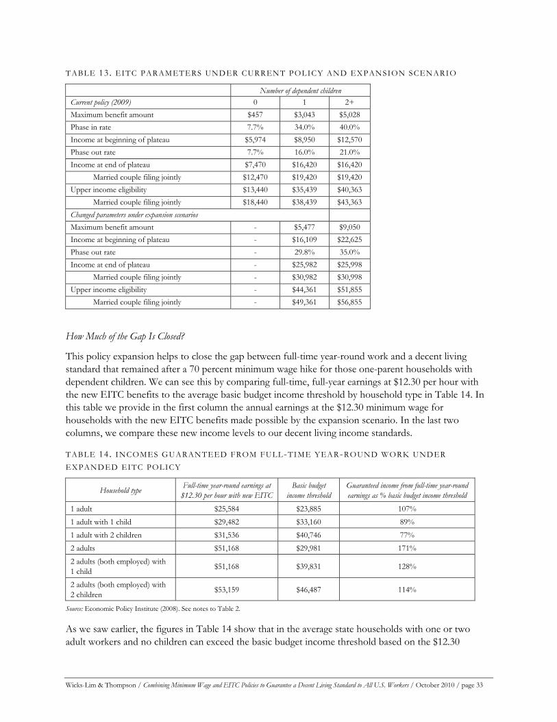
TABLE 13. EITC PARAMETERS UNDER CURRENT POLICY AND EXPANSION SCENARIO Number of dependent children Current policy (2009) 0 1 2+ Maximum benefit amount $457 $3,043 $5,028 Phase in rate 7.7% 34.0% 40.0% Income at beginning of plateau $5,974 $8,950 $12,570 Phase out rate 7.7% 16.0% 21.0% Income at end of plateau $7,470 $16,420 $16,420 Married couple filing jointly $12,470 $19,420 $19,420 Upper income eligibility $13,440 $35,439 $40,363 Married couple filing jointly $18,440 $38,439 $43,363 Changed parameters under expansion scenarios Maximum benefit amount - $5,477 $9,050 Income at beginning of plateau - $16,109 $22,625 Phase out rate - 29.8% 35.0% Income at end of plateau - $25,982 $25,998 Married couple filing jointly - $30,982 $30,998 Upper income eligibility - $44,361 $51,855 Married couple filing jointly - $49,361 $56,855
How Much of the Gap Is Closed?
This policy expansion helps to close the gap between full-time year-round work and a decent living standard that remained after a 70 percent minimum wage hike for those one-parent households with dependent children. We can see this by comparing full-time, full-year earnings at $12.30 per hour with the new EITC benefits to the average basic budget income threshold by household type in Table 14. In this table we provide in the first column the annual earnings at the $12.30 minimum wage for households with the new EITC benefits made possible by the expansion scenario. In the last two columns, we compare these new income levels to our decent living income standards.
TABLE 14. INCOMES GUARANTEED FROM FULL-TIME YEAR-ROUND WORK UNDER EXPANDED EITC POLICY
Household type Full-time year-round earnings at $12.30 per hour with new EITC
Basic budget income threshold
Guaranteed income from full-time year-round earnings as % basic budget income threshold
1 adult $25,584 $23,885 107% 1 adult with 1 child $29,482 $33,160 89% 1 adult with 2 children $31,536 $40,746 77% 2 adults $51,168 $29,981 171% 2 adults (both employed) with 1 child $51,168 $39,831 128%
2 adults (both employed) with 2 children $53,159 $46,487 114%
Source: Economic Policy Institute (2008). See notes to Table 2.
As we saw earlier, the figures in Table 14 show that in the average state households with one or two adult workers and no children can exceed the basic budget income threshold based on the $12.30
Wicks-Lim & Thompson / Combining Minimum Wage and EITC Policies to Guarantee a Decent Living Standard to All U.S. Workers / October 2010 / page 33

Wicks-Lim & Thompson / Combining Minimum Wage and EITC Policies to Guarantee a Decent Living Standard to All U.S. Workers / October 2010 / page 34
minimum wage earnings alone. The situation is the same for households in which there are two working adults and one or two dependent children.
For the other household types (one adult earner and one or two dependent children), the EITC helps to close the gap substantially between minimum wage earnings and the basic budget income thresholds in the typical state. If we compare the figures in this table to those in Table 11 above, we can see that the gap for 1 adult/1 child households fell from 23 percent to 11 percent and for 1 adult/2 children households from 37 percent to 23 percent.
To examine how these gaps vary across areas, we focus our attention again on 1 adult/2 children households that face the largest challenge in achieving sufficient income to meet our decent living standard. In Table 15 we provide figures of minimum wage earnings plus new EITC benefits, and a comparison between the earnings and new benefits to the basic budget income threshold for our three representative areas, Wyoming, Illinois, and the District of Columbia.44
TABLE 15. INCOMES GUARANTEED FROM FULL-TIME YEAR-ROUND WORK UNDER THE EXPANDED EITC POLICY COMPARED TO BASIC BUDGET INCOME THRESHOLDS FOR A FAMILY OF THREE (1 ADULT, 2 CHILDREN) IN THREE REPRESENTATIVE AREAS
Area Full-time year-round earnings after 70% minimum wage hike and new
EITC benefits
Basic budget income
threshold
Guaranteed income from full-time year-round earnings as % basic budget income threshold
Wyoming $ 31,536 $ 30,453 104% Illinois $ 34,294 $ 43,351 79%
District of Columbia $ 37,049 $ 65,631 56%
Source: Economic Policy Institute (2008). See notes to Table 2. State-by-state figures are available upon request from authors.
For households with one adult and two children, the combined policies will succeed in moving a family of three to the basic budget income threshold in the state with the lowest living costs, Wyoming. For a state with more typical living costs, such Illinois, a 21 percent gap remains. This is a smaller, yet still significant gap, than the 31 percent that remained after the minimum wage hike alone.
Most low-income households in which there is only one earner and a least one dependent child will need more support than what the minimum wage hike and expanded EITC credit offer. These households have the significant disadvantage of having only one worker to cover the expenses of raising kids while, at the same time, working away from the home.
Childcare expenses alone typically make up more than 20 percent of the budgets of low-income households with young children. A full childcare subsidy therefore would nearly fill the entire 23 percent gap left between full-time year-round minimum earnings and the basic budget income threshold for a single earner household with two children living in an average state (see Table 14).
There are some promising state programs that can help to reduce child care expenses substantially for families with incomes up to 200 percent of the federal poverty income threshold. For example, the National Women’s Law Center estimates that in Illinois, subsidies for a family with one child in childcare and income equal to 150 percent of the official poverty line can bring their expenses down to co-pays equal to about seven percent of the family’s income (Shulman and Blank, 2009). A childcare subsidy 44 A listing of state-by-state figures (including figures for D.C.) is available from the authors up request.
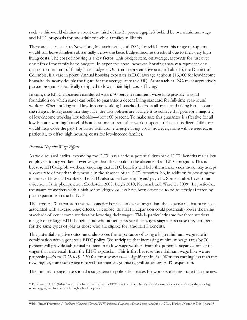
Wicks-Lim & Thompson / Combining Minimum Wage and EITC Policies to Guarantee a Decent Living Standard to All U.S. Workers / October 2010 / page 35
such as this would eliminate about one-third of the 21 percent gap left behind by our minimum wage and EITC proposals for one-adult one-child families in Illinois.
There are states, such as New York, Massachusetts, and D.C., for which even this range of support would still leave families substantially below the basic budget income threshold due to their very high living costs. The cost of housing is a key factor. This budget item, on average, accounts for just over one-fifth of the family basic budgets. In expensive areas, however, housing costs can represent one-quarter to one-third of family basic budgets. Our third representative area in Table 15, the District of Columbia, is a case in point. Annual housing expenses in D.C. average at about $16,000 for low-income households, nearly double the figure for the average state ($9,000). Areas such as D.C. must aggressively pursue programs specifically designed to lower their high cost of living.
In sum, the EITC expansion combined with a 70 percent minimum wage hike provides a solid foundation on which states can build to guarantee a decent living standard for full-time year-round workers. When looking at all low-income working households across all areas, and taking into account the range of living costs that they face, the two policies are sufficient to achieve this goal for a majority of low-income working households—about 60 percent. To make sure this guarantee is effective for all low-income working households at least one or two other work supports such as subsidized child care would help close the gap. For states with above-average living costs, however, more will be needed, in particular, to offset high housing costs for low-income families. Potential Negative Wage Effects
As we discussed earlier, expanding the EITC has a serious potential drawback. EITC benefits may allow employers to pay workers lower wages than they could in the absence of an EITC program. This is because EITC-eligible workers, knowing that EITC benefits will help them make ends meet, may accept a lower rate of pay than they would in the absence of an EITC program. So, in addition to boosting the incomes of low-paid workers, the EITC also subsidizes employers’ payrolls. Some studies have found evidence of this phenomenon (Rothstein 2008, Leigh 2010, Neumark and Wascher 2009). In particular, the wages of workers with a high school degree or less have been observed to be adversely affected by past expansions in the EITC.45
The large EITC expansion that we consider here is somewhat larger than the expansions that have been associated with adverse wage effects. Therefore, this EITC expansion could potentially lower the living standards of low-income workers by lowering their wages. This is particularly true for those workers ineligible for large EITC benefits, but who nonetheless see their wages stagnate because they compete for the same types of jobs as those who are eligible for large EITC benefits.
This potential negative outcome underscores the importance of using a high minimum wage rate in combination with a generous EITC policy. We anticipate that increasing minimum wage rates by 70 percent will provide substantial protection to low-wage workers from the potential negative impact on wages that may result from the EITC expansion. This is first because the minimum wage hike we are proposing—from $7.25 to $12.30 for most workers—is significant in size. Workers earning less than the new, higher, minimum wage rate will see their wages rise regardless of any EITC expansion.
The minimum wage hike should also generate ripple-effect raises for workers earning more than the new
45 For example, Leigh (2010) found that a 10 percent increase in EITC benefits reduced hourly wages by two percent for workers with only a high school degree, and five percent for high school dropouts.
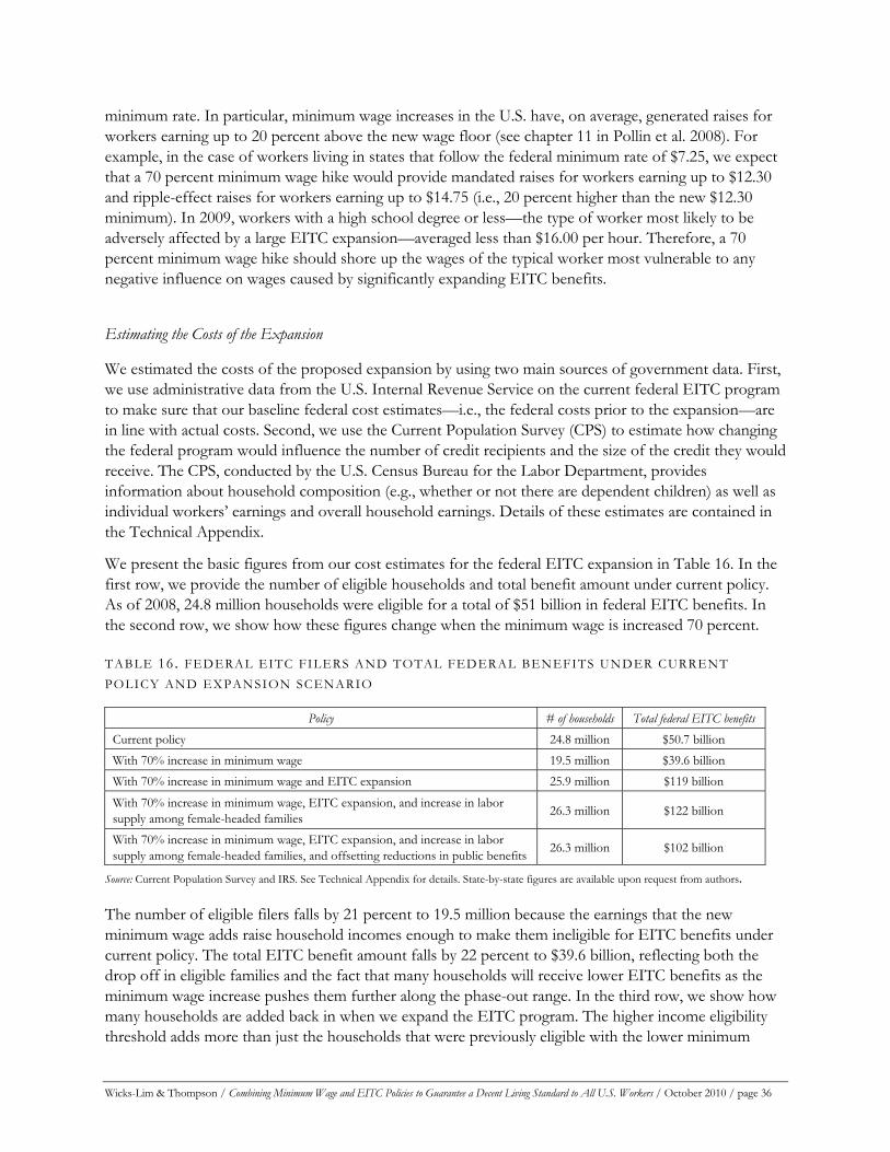
minimum rate. In particular, minimum wage increases in the U.S. have, on average, generated raises for workers earning up to 20 percent above the new wage floor (see chapter 11 in Pollin et al. 2008). For example, in the case of workers living in states that follow the federal minimum rate of $7.25, we expect that a 70 percent minimum wage hike would provide mandated raises for workers earning up to $12.30 and ripple-effect raises for workers earning up to $14.75 (i.e., 20 percent higher than the new $12.30 minimum). In 2009, workers with a high school degree or less—the type of worker most likely to be adversely affected by a large EITC expansion—averaged less than $16.00 per hour. Therefore, a 70 percent minimum wage hike should shore up the wages of the typical worker most vulnerable to any negative influence on wages caused by significantly expanding EITC benefits.
Estimating the Costs of the Expansion
We estimated the costs of the proposed expansion by using two main sources of government data. First, we use administrative data from the U.S. Internal Revenue Service on the current federal EITC program to make sure that our baseline federal cost estimates—i.e., the federal costs prior to the expansion—are in line with actual costs. Second, we use the Current Population Survey (CPS) to estimate how changing the federal program would influence the number of credit recipients and the size of the credit they would receive. The CPS, conducted by the U.S. Census Bureau for the Labor Department, provides information about household composition (e.g., whether or not there are dependent children) as well as individual workers’ earnings and overall household earnings. Details of these estimates are contained in the Technical Appendix.
We present the basic figures from our cost estimates for the federal EITC expansion in Table 16. In the first row, we provide the number of eligible households and total benefit amount under current policy. As of 2008, 24.8 million households were eligible for a total of $51 billion in federal EITC benefits. In the second row, we show how these figures change when the minimum wage is increased 70 percent.
TABLE 16. FEDERAL EITC FILERS AND TOTAL FEDERAL BENEFITS UNDER CURRENT POLICY AND EXPANSION SCENARIO
Policy # of households Total federal EITC benefits Current policy 24.8 million $50.7 billion With 70% increase in minimum wage 19.5 million $39.6 billion With 70% increase in minimum wage and EITC expansion 25.9 million $119 billion
With 70% increase in minimum wage, EITC expansion, and increase in labor supply among female-headed families 26.3 million $122 billion
With 70% increase in minimum wage, EITC expansion, and increase in labor supply among female-headed families, and offsetting reductions in public benefits 26.3 million $102 billion
Source: Current Population Survey and IRS. See Technical Appendix for details. State-by-state figures are available upon request from authors.
The number of eligible filers falls by 21 percent to 19.5 million because the earnings that the new minimum wage adds raise household incomes enough to make them ineligible for EITC benefits under current policy. The total EITC benefit amount falls by 22 percent to $39.6 billion, reflecting both the drop off in eligible families and the fact that many households will receive lower EITC benefits as the minimum wage increase pushes them further along the phase-out range. In the third row, we show how many households are added back in when we expand the EITC program. The higher income eligibility threshold adds more than just the households that were previously eligible with the lower minimum
Wicks-Lim & Thompson / Combining Minimum Wage and EITC Policies to Guarantee a Decent Living Standard to All U.S. Workers / October 2010 / page 36
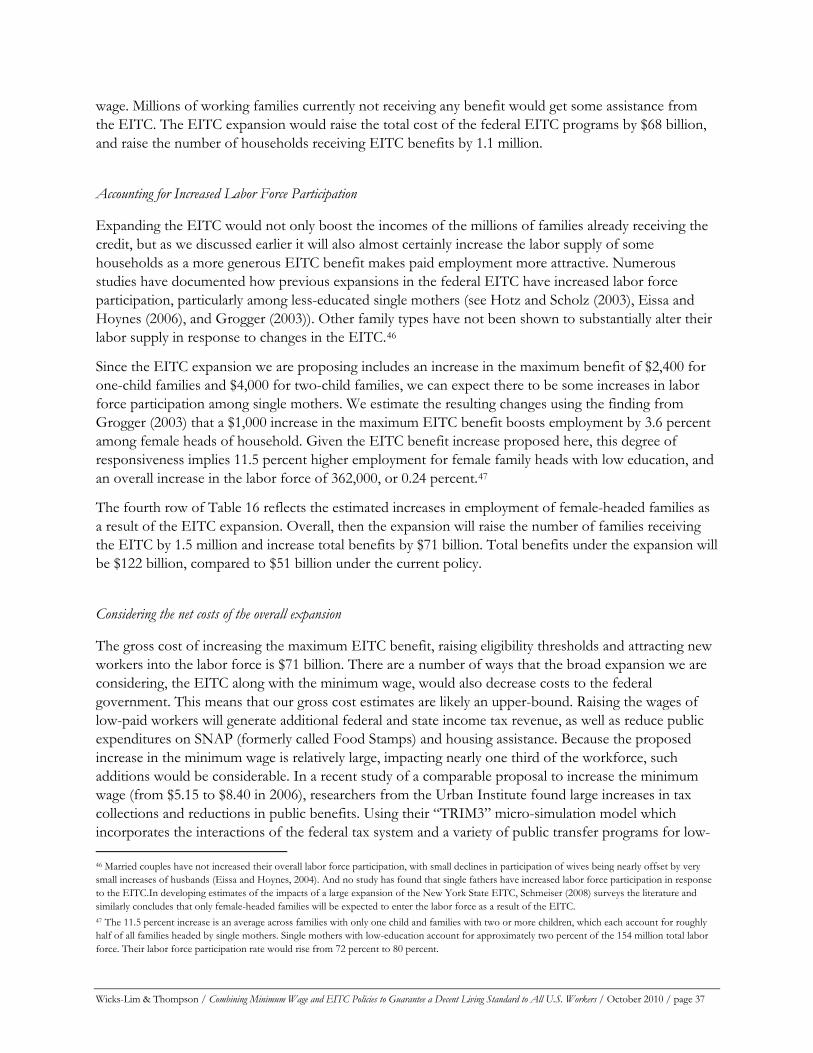
Wicks-Lim & Thompson / Combining Minimum Wage and EITC Policies to Guarantee a Decent Living Standard to All U.S. Workers / October 2010 / page 37
wage. Millions of working families currently not receiving any benefit would get some assistance from the EITC. The EITC expansion would raise the total cost of the federal EITC programs by $68 billion, and raise the number of households receiving EITC benefits by 1.1 million.
Accounting for Increased Labor Force Participation
Expanding the EITC would not only boost the incomes of the millions of families already receiving the credit, but as we discussed earlier it will also almost certainly increase the labor supply of some households as a more generous EITC benefit makes paid employment more attractive. Numerous studies have documented how previous expansions in the federal EITC have increased labor force participation, particularly among less-educated single mothers (see Hotz and Scholz (2003), Eissa and Hoynes (2006), and Grogger (2003)). Other family types have not been shown to substantially alter their labor supply in response to changes in the EITC.46
Since the EITC expansion we are proposing includes an increase in the maximum benefit of $2,400 for one-child families and $4,000 for two-child families, we can expect there to be some increases in labor force participation among single mothers. We estimate the resulting changes using the finding from Grogger (2003) that a $1,000 increase in the maximum EITC benefit boosts employment by 3.6 percent among female heads of household. Given the EITC benefit increase proposed here, this degree of responsiveness implies 11.5 percent higher employment for female family heads with low education, and an overall increase in the labor force of 362,000, or 0.24 percent.47
The fourth row of Table 16 reflects the estimated increases in employment of female-headed families as a result of the EITC expansion. Overall, then the expansion will raise the number of families receiving the EITC by 1.5 million and increase total benefits by $71 billion. Total benefits under the expansion will be $122 billion, compared to $51 billion under the current policy.
Considering the net costs of the overall expansion
The gross cost of increasing the maximum EITC benefit, raising eligibility thresholds and attracting new workers into the labor force is $71 billion. There are a number of ways that the broad expansion we are considering, the EITC along with the minimum wage, would also decrease costs to the federal government. This means that our gross cost estimates are likely an upper-bound. Raising the wages of low-paid workers will generate additional federal and state income tax revenue, as well as reduce public expenditures on SNAP (formerly called Food Stamps) and housing assistance. Because the proposed increase in the minimum wage is relatively large, impacting nearly one third of the workforce, such additions would be considerable. In a recent study of a comparable proposal to increase the minimum wage (from $5.15 to $8.40 in 2006), researchers from the Urban Institute found large increases in tax collections and reductions in public benefits. Using their “TRIM3” micro-simulation model which incorporates the interactions of the federal tax system and a variety of public transfer programs for low- 46 Married couples have not increased their overall labor force participation, with small declines in participation of wives being nearly offset by very small increases of husbands (Eissa and Hoynes, 2004). And no study has found that single fathers have increased labor force participation in response to the EITC.In developing estimates of the impacts of a large expansion of the New York State EITC, Schmeiser (2008) surveys the literature and similarly concludes that only female-headed families will be expected to enter the labor force as a result of the EITC. 47 The 11.5 percent increase is an average across families with only one child and families with two or more children, which each account for roughly half of all families headed by single mothers. Single mothers with low-education account for approximately two percent of the 154 million total labor force. Their labor force participation rate would rise from 72 percent to 80 percent.
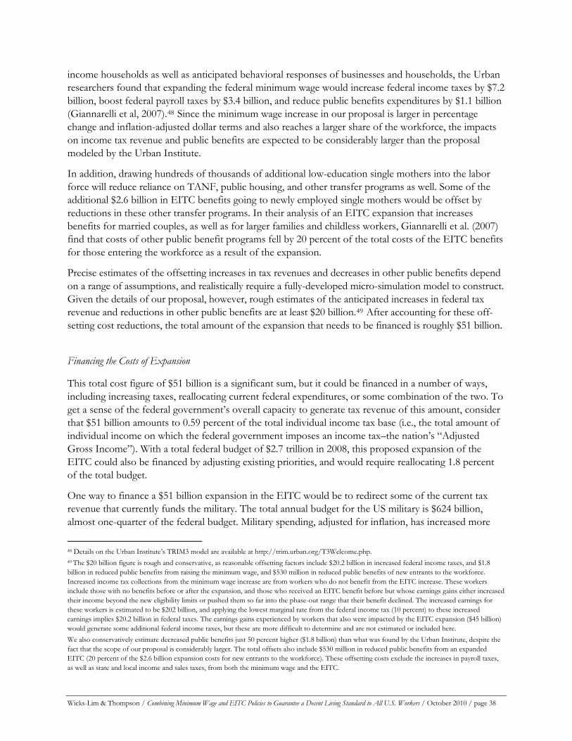
Wicks-Lim & Thompson / Combining Minimum Wage and EITC Policies to Guarantee a Decent Living Standard to All U.S. Workers / October 2010 / page 38
income households as well as anticipated behavioral responses of businesses and households, the Urban researchers found that expanding the federal minimum wage would increase federal income taxes by $7.2 billion, boost federal payroll taxes by $3.4 billion, and reduce public benefits expenditures by $1.1 billion (Giannarelli et al, 2007).48 Since the minimum wage increase in our proposal is larger in percentage change and inflation-adjusted dollar terms and also reaches a larger share of the workforce, the impacts on income tax revenue and public benefits are expected to be considerably larger than the proposal modeled by the Urban Institute.
In addition, drawing hundreds of thousands of additional low-education single mothers into the labor force will reduce reliance on TANF, public housing, and other transfer programs as well. Some of the additional $2.6 billion in EITC benefits going to newly employed single mothers would be offset by reductions in these other transfer programs. In their analysis of an EITC expansion that increases benefits for married couples, as well as for larger families and childless workers, Giannarelli et al. (2007) find that costs of other public benefit programs fell by 20 percent of the total costs of the EITC benefits for those entering the workforce as a result of the expansion.
Precise estimates of the offsetting increases in tax revenues and decreases in other public benefits depend on a range of assumptions, and realistically require a fully-developed micro-simulation model to construct. Given the details of our proposal, however, rough estimates of the anticipated increases in federal tax revenue and reductions in other public benefits are at least $20 billion.49 After accounting for these off-setting cost reductions, the total amount of the expansion that needs to be financed is roughly $51 billion.
Financing the Costs of Expansion
This total cost figure of $51 billion is a significant sum, but it could be financed in a number of ways, including increasing taxes, reallocating current federal expenditures, or some combination of the two. To get a sense of the federal government’s overall capacity to generate tax revenue of this amount, consider that $51 billion amounts to 0.59 percent of the total individual income tax base (i.e., the total amount of individual income on which the federal government imposes an income tax–the nation’s “Adjusted Gross Income”). With a total federal budget of $2.7 trillion in 2008, this proposed expansion of the EITC could also be financed by adjusting existing priorities, and would require reallocating 1.8 percent of the total budget.
One way to finance a $51 billion expansion in the EITC would be to redirect some of the current tax revenue that currently funds the military. The total annual budget for the US military is $624 billion, almost one-quarter of the federal budget. Military spending, adjusted for inflation, has increased more
48 Details on the Urban Institute’s TRIM3 model are available at http://trim.urban.org/T3Welcome.php. 49 The $20 billion figure is rough and conservative, as reasonable offsetting factors include $20.2 billion in increased federal income taxes, and $1.8 billion in reduced public benefits from raising the minimum wage, and $530 million in reduced public benefits of new entrants to the workforce. Increased income tax collections from the minimum wage increase are from workers who do not benefit from the EITC increase. These workers include those with no benefits before or after the expansion, and those who received an EITC benefit before but whose earnings gains either increased their income beyond the new eligibility limits or pushed them so far into the phase-out range that their benefit declined. The increased earnings for these workers is estimated to be $202 billion, and applying the lowest marginal rate from the federal income tax (10 percent) to these increased earnings implies $20.2 billion in federal taxes. The earnings gains experienced by workers that also were impacted by the EITC expansion ($45 billion) would generate some additional federal income taxes, but these are more difficult to determine and are not estimated or included here. We also conservatively estimate decreased public benefits just 50 percent higher ($1.8 billion) than what was found by the Urban Institute, despite the fact that the scope of our proposal is considerably larger. The total offsets also include $530 million in reduced public benefits from an expanded EITC (20 percent of the $2.6 billion expansion costs for new entrants to the workforce). These offsetting costs exclude the increases in payroll taxes, as well as state and local income and sales taxes, from both the minimum wage and the EITC.
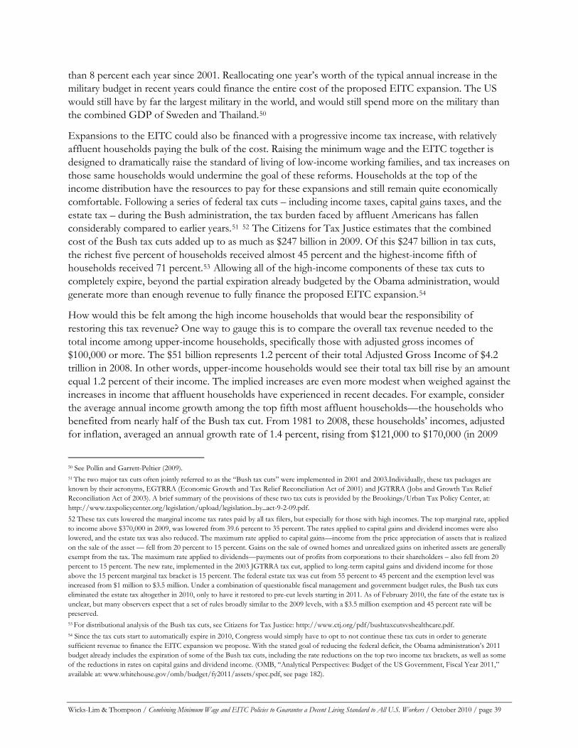
Wicks-Lim & Thompson / Combining Minimum Wage and EITC Policies to Guarantee a Decent Living Standard to All U.S. Workers / October 2010 / page 39
than 8 percent each year since 2001. Reallocating one year’s worth of the typical annual increase in the military budget in recent years could finance the entire cost of the proposed EITC expansion. The US would still have by far the largest military in the world, and would still spend more on the military than the combined GDP of Sweden and Thailand.50
Expansions to the EITC could also be financed with a progressive income tax increase, with relatively affluent households paying the bulk of the cost. Raising the minimum wage and the EITC together is designed to dramatically raise the standard of living of low-income working families, and tax increases on those same households would undermine the goal of these reforms. Households at the top of the income distribution have the resources to pay for these expansions and still remain quite economically comfortable. Following a series of federal tax cuts – including income taxes, capital gains taxes, and the estate tax – during the Bush administration, the tax burden faced by affluent Americans has fallen considerably compared to earlier years.51 52 The Citizens for Tax Justice estimates that the combined cost of the Bush tax cuts added up to as much as $247 billion in 2009. Of this $247 billion in tax cuts, the richest five percent of households received almost 45 percent and the highest-income fifth of households received 71 percent.53 Allowing all of the high-income components of these tax cuts to completely expire, beyond the partial expiration already budgeted by the Obama administration, would generate more than enough revenue to fully finance the proposed EITC expansion.54
How would this be felt among the high income households that would bear the responsibility of restoring this tax revenue? One way to gauge this is to compare the overall tax revenue needed to the total income among upper-income households, specifically those with adjusted gross incomes of $100,000 or more. The $51 billion represents 1.2 percent of their total Adjusted Gross Income of $4.2 trillion in 2008. In other words, upper-income households would see their total tax bill rise by an amount equal 1.2 percent of their income. The implied increases are even more modest when weighed against the increases in income that affluent households have experienced in recent decades. For example, consider the average annual income growth among the top fifth most affluent households—the households who benefited from nearly half of the Bush tax cut. From 1981 to 2008, these households’ incomes, adjusted for inflation, averaged an annual growth rate of 1.4 percent, rising from $121,000 to $170,000 (in 2009
50 See Pollin and Garrett-Peltier (2009). 51 The two major tax cuts often jointly referred to as the “Bush tax cuts” were implemented in 2001 and 2003.Individually, these tax packages are known by their acronyms, EGTRRA (Economic Growth and Tax Relief Reconciliation Act of 2001) and JGTRRA (Jobs and Growth Tax Relief Reconciliation Act of 2003). A brief summary of the provisions of these two tax cuts is provided by the Brookings/Urban Tax Policy Center, at: http://www.taxpolicycenter.org/legislation/upload/legislation_by_act-9-2-09.pdf. 52 These tax cuts lowered the marginal income tax rates paid by all tax filers, but especially for those with high incomes. The top marginal rate, applied to income above $370,000 in 2009, was lowered from 39.6 percent to 35 percent. The rates applied to capital gains and dividend incomes were also lowered, and the estate tax was also reduced. The maximum rate applied to capital gains—income from the price appreciation of assets that is realized on the sale of the asset — fell from 20 percent to 15 percent. Gains on the sale of owned homes and unrealized gains on inherited assets are generally exempt from the tax. The maximum rate applied to dividends—payments out of profits from corporations to their shareholders – also fell from 20 percent to 15 percent. The new rate, implemented in the 2003 JGTRRA tax cut, applied to long-term capital gains and dividend income for those above the 15 percent marginal tax bracket is 15 percent. The federal estate tax was cut from 55 percent to 45 percent and the exemption level was increased from $1 million to $3.5 million. Under a combination of questionable fiscal management and government budget rules, the Bush tax cuts eliminated the estate tax altogether in 2010, only to have it restored to pre-cut levels starting in 2011. As of February 2010, the fate of the estate tax is unclear, but many observers expect that a set of rules broadly similar to the 2009 levels, with a $3.5 million exemption and 45 percent rate will be preserved. 53 For distributional analysis of the Bush tax cuts, see Citizens for Tax Justice: http://www.ctj.org/pdf/bushtaxcutsvshealthcare.pdf. 54 Since the tax cuts start to automatically expire in 2010, Congress would simply have to opt to not continue these tax cuts in order to generate sufficient revenue to finance the EITC expansion we propose. With the stated goal of reducing the federal deficit, the Obama administration’s 2011 budget already includes the expiration of some of the Bush tax cuts, including the rate reductions on the top two income tax brackets, as well as some of the reductions in rates on capital gains and dividend income. (OMB, “Analytical Perspectives: Budget of the US Government, Fiscal Year 2011,” available at: www.whitehouse.gov/omb/budget/fy2011/assets/spec.pdf, see page 182).
Wicks-Lim & Thompson / Combining Minimum Wage and EITC Policies to Guarantee a Decent Living Standard to All U.S. Workers / October 2010 / page 40
dollars).55 If these households paid for the federal EITC expansion with 1.2 percent of their income, this would be equal to slightly less than one year’s worth of real income growth. In other words, their standard of living would remain steady for one year, and in subsequent years these households would their see their living standards rise as before.
In addition to these options, the EITC expansion could be financed through other types of tax increases (a financial transactions tax, for example) or some combination of tax and spending changes.56 Regardless of the details, funding a major expansion of the EITC is economically feasible, with the real question remaining one of political will. The decision to dedicate funding to this expansion – as opposed to some other policy priority – also becomes easier when the economy is growing rapidly. Faster economic growth generates more federal tax revenue for all purposes. A one percentage point drop in the unemployment rate alone would generate about $90 billion in government revenues (Pollin, 2010, 13). Lower unemployment means greater tax revenue from the earnings of employed workers as well as less spending on government programs to support the unemployed. So, as the economy recovers in the coming years, especially if federal policy makers decide to take more aggressive action to bring down unemployment, there will be additional revenue that can be used to finance an initiative like this major expansion of the EITC.
55 Mean household incomes received by each fifth and top 5 percent of households are published by the U.S. Census Bureau. http://www.census.gov/hhes/www/income/histinc/inchhtoc.html; accessed Feb. 22, 2010. This 1.4 percent figure may seem low given the relatively large rates of income growth experienced by high income households documented by Thomas Piketty and Emmanuel Saez (see, for example, Piketty and Saez, 2007). However, the high rates of income growth are concentrated among the super-rich, e.g., the average annual income of the top 0.01 percent of households grew at a pace of 7 percent per year between 1980 and 2008. The 1.4 percent income growth figure that we report here is consistent with the income data Piketty and Saez report for households with incomes comparable to the top fifth of households. 56 For details on financial transaction taxes, see Baker, Pollin, McArthur, and Sherman (2009).
Wicks-Lim & Thompson / Combining Minimum Wage and EITC Policies to Guarantee a Decent Living Standard to All U.S. Workers / October 2010 / page 41
THE OTHER HALF OF THE CHALLENGE: GETTING TO FULL EMPLOYMENT
Our policy proposals address one of the crucial elements of an economic policy framework that aggressively pursues the goal of raising all U.S. households to a decent living standard: decent pay. A 70 percent increase in the minimum wage and a more than doubling of the existing federal EITC program would put in place a guarantee that full-time year-round work would support a decent living standard for the majority of low-income working households.
The other crucial element is creating a full employment economy. Clearly, neither the minimum wage nor EITC programs will benefit low-income families who have no household members in the workforce. Moreover, even if household members have jobs, the degree to which these policies can move families toward a decent living standard hinges on the number of hours they actually work.
We can see how the issue of adequate employment impacts the ability of our policy proposals to lift low income families to a decent living standard by estimating how much the proportion of families with incomes below the basic budget threshold would fall given their current employment status. We estimate that our proposed expansion will reduce the percentage of low income families with inadequate incomes from 26 percent to 22 percent.
On the one hand, this drop-off of four percentage points is striking. Consider that over the nine-year period that the Economic Policy Institute has been publishing these basic budget income thresholds for families with young children, from 1998 to 2007, the percentage of individuals falling below the threshold has actually risen by about one percentage point.57 Therefore our policy expansion clearly addresses a substantial barrier to achieving a decent living standard.
On the other hand, the four percentage point reduction is much smaller than what it would be if the adults in low income households had full-time year-round employment. In fact, the average household head of a low-income working family worked about 1,420 hours annually in 2005-07—significantly less than full-time, year-round (2,080 hours).58 If all household heads and their spouses (if present) in low income households worked full-time year round, we would expect a drop off of close to 15 percentage points, so that the percent of low-income households would fall from 26 percent to 11 percent. Inadequate employment is clearly a significant barrier to families achieving a decent living standard.
Neither the minimum wage nor EITC policies are, in and of themselves, designed to serve as major engines of economy-wide job creation. Recall the debate over how minimum wage laws affect employment. As we discussed above, there is no strong evidence that minimum wage or living wage laws reduce work schedules or employment levels. At the same time, there is no evidence that minimum wage laws cause a significant boost in employment. EITC policies, in contrast, can draw more workers to participate in the labor force by making paid employment more attractive, especially for low-income single mothers. The availability of job openings however determines whether this increase in labor force participation results in higher employment rates.
57 The first published figure by Boushey et al. (2001) was estimate for 1997-1999. The last published figure by Lin and Bernstein (2008) was for 2007. Their level figures (29.8 percent in 2007 and 28.9 percent for 1997-1999) are similar but slightly different from our measure. This is primarily because EPI analyses treat inter-generational families living under one roof as a single family unit and assess the percent of these units with incomes below the basic budget income threshold. We, in contrast, estimate the percentage of families with incomes below the basic budget income threshold and treat families who live under the same roof but file taxes separately as separate family units. 58 See Technical Appendix Table A.7 for details on the demographics of low income working households.

Wicks-Lim & Thompson / Combining Minimum Wage and EITC Policies to Guarantee a Decent Living Standard to All U.S. Workers / October 2010 / page 42
Instead, the overall employment level is only effectively addressed by whether the economy is operating at a high level of activity. Policy levers that influence economic activity include those that direct government spending and taxation, and the flow of credit through our economy. The most recent recession demonstrates this in a dramatic way. Neither the minimum wage nor EITC policies changed in any significant way when the U.S. economy collapsed in 2008, raising the unemployment rate to ten percent.59 Rather, the most apparent cause of this severe downturn is that the U.S. economy lost the one engine that had kept it going since the late 1990s: the bubble in the housing market.
However, there is an important way through which higher minimum wages and an expanded EITC can promote a more stable economy with expanded employment opportunities at the macroeconomic level. This is through reducing income inequality in the U.S. economy. A more egalitarian income distribution, in turn, expands the level of consumer expenditures, and thus of business opportunities to successfully sell products within the U.S. economy. Thus, a 2008 study by researchers at the Federal Reserve Bank of Boston found that consumer spending on durable goods—new cars and trucks in particular—rises in response to a minimum wage increase among households that substantially depend on minimum wage jobs.60
The general lesson here is clear. The sharp rise in income inequality over roughly the last three decades has helped the richest households leverage an increasingly larger amount of income for speculative investments. This rise in speculative investing contributed to the bubble in the housing market that eventually burst and propelled the U.S. into the Great Recession. By the same token, by supporting a greater level of income equality, higher minimum wage rates and generous EITC benefits can help to maintain a stable and robust level of consumer demand that would, in turn, encourage productive, rather than speculative, investments. These can be important contributors toward building an egalitarian and sustainable recovery from the Great Recession.
Considered most broadly, our policy proposals combined with an effort to achieve full employment would produce, for the first time in U.S. history, an economy in which the majority of those who are willing and able to work would be guaranteed, at minimum, a decent standard of living for themselves and their families.
59 One question that we have not addressed is whether a relatively high minimum wage would make recessions worse. In fact, there is no strong evidence that a higher minimum wage would make it more difficult for businesses to survive recessions. This is because firms typically do not use wage cuts as a way to buoy their business during an economic downturn. Therefore, a higher minimum wage standard would not block businesses from taking actions that they would otherwise to adjust to a fall off in business. Instead, firms usually cut costs during recessions through layoffs. Truman Bewley’s 1999 book, Why Wages Don’t Fall During a Recession, provides unique documentation of the reasons why firms do not lower wages during an economic downturn. In this book, Bewley describes his extensive and detailed interviews with managers from a variety of firms during the recessions of the early 1990s about how they adjust to downturns. From these, he identifies three major reasons why layoffs are preferred to wage reductions. First, pay cuts do not generate enough savings to avoid layoffs. In other words, recessions require large adjustments to how a business is operating and wage cuts only result in minor changes. Second, pay cuts hurt worker morale. As a result, this type of cost savings can cause workers to perform their jobs less effectively and make it even more difficult for firms to keep afloat during a recession. A third reason is that wage cuts do not address the fundamental problem facing firms: the lack of demand for their products. The price reductions that could be passed from wage cuts are unlikely to raise the demand for their product in any significant way in the face of an overall economic slowdown. During the current recession, arguably the most severe since the Great Depression, there is evidence that some businesses have turned to wage-cutting to adjust to the large and rapid fall off in economic activity in 2008. But again, this is an example of how this recession is the exception that proves the rule. The fact that businesses are turning to wage cuts at all is noted precisely because of such actions are so rare, and as a sign of the severe downswing of the recession. 60 Aaronson, Agarwal, and French (2008).

Wicks-Lim & Thompson / Combining Minimum Wage and EITC Policies to Guarantee a Decent Living Standard to All U.S. Workers / October 2010 / page 43
CONCLUSION
Current policies do not guarantee a decent living standard for employed working people and their families. On average, there exists a 63 percent gap between what is guaranteed by a full-time year-round job at the $7.25 federal minimum wage and the income required to support what can reasonably be called a decent living standard for a family of three, as an example.61 Given the size of the gap, developing effective measures for closing it may seem daunting.
This paper makes clear that we can indeed eliminate this gap for the majority of low income working households and significantly shrink this gap for remaining households. The U.S. economy has the resources needed to support an ambitious set of policy changes that would set a solid foundation for guaranteeing a decent living standard for workers and their families.
Specifically, we conservatively estimate that firms could absorb a 70 percent minimum wage hike by using just two adjustment mechanisms: raising prices and relying on future economic growth to buoy their business activity. In this exercise we assume an annual growth rate of 3.0 percent—a growth rate reasonably within reach once the U.S. economy emerges from the current economic downturn. If businesses adjusted in other ways, such as redistributing income within the firm from profits to low-wage workers or from high-wage workers to low-wage workers, they could either absorb a higher minimum wage increase or rely less on prices increases or economic growth.
In most states a minimum wage increase of this size would be equal, in today’s dollars, to $12.30, a 70 percent raise from the federal rate of $7.25. Our examination of the industry that would face the largest challenges in adjusting to a minimum wage hike, the restaurant industry, indicates that it could cover the cost increases from a 70 percent increase. Restaurants could do this with a combination of generating additional revenue from modestly higher prices supported by the usual increase in business activity and cost-savings from higher worker productivity. A minimum wage at this level is sufficient to provide a decent living standard for households with two earners and one earner households with no dependent children living in states with average living costs.
Households with children that depend on one earner and households in high-cost areas will need additional support. We propose a large expansion of the current federal EITC program to help fill this gap. Our proposal includes an 80 percent increase in the maximum benefit and extending benefits to households earning up to 300 percent of the official poverty line.
The expanded EITC benefits would work in conjunction with a minimum wage hike to bring one-earner households with children much closer to their basic budget income thresholds. In fact, in Wyoming, the lowest cost state in the country, all household types would be guaranteed a decent living standard with these two proposals in place. If we now consider all low-income working households across all states, our combined policy proposals would guarantee that the majority—60 percent—could achieve a decent living standard through full-time year-round work. The remaining 40 percent of low-income working families live in high-cost areas or depend on one earner to raise children, and will require additional support. These policies, however, reduces considerably the amount of other supports these low-income working families would need.
61 Family of three includes one adult and two children.

Taxes targeted at upper-income households could fund this expansion of EITC benefits. If financed this way, households with incomes in excess of $100,000 would experience an increase in their tax bill equal to 1.2 percent of their income. This is equivalent to just under one year’s worth of the inflation-adjusted income growth affluent households have experienced in recent decades. This would mean that over the next five years their average inflation-adjusted income would rise from a current average of about $170,000 to $180,000, rather than from $170,000 to $182,000 (in 2009 dollars). Alternatively, the expansion could be financed by reallocating just one year’s worth of the typical increase in the military budget from recent years. The US would still have by far the largest military in the world. A healthier economy with a lower unemployment rate would raise federal revenue and lower federal expenses more than enough to support our proposed expansions.
The U.S. economy is a highly productive, yet highly unequal economy. We conclude from our analysis that the U.S. economy can marshal much more in resources to guarantee a decent living standard for workers and their families than it does currently. This report provides a map of how we can use existing economic policies, the minimum wage and the EITC program, to do this.
Wicks-Lim & Thompson / Combining Minimum Wage and EITC Policies to Guarantee a Decent Living Standard to All U.S. Workers / October 2010 / page 44
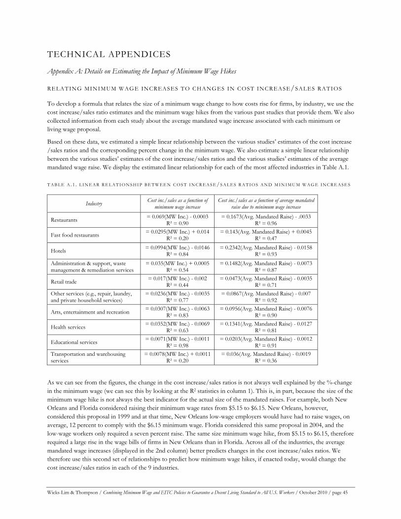
TECHNICAL APPENDICES
Appendix A: Details on Estimating the Impact of Minimum Wage Hikes
RELATING MINIMUM WAGE INCREASES TO CHANGES IN COST INCREASE/SALES RATIOS
To develop a formula that relates the size of a minimum wage change to how costs rise for firms, by industry, we use the cost increase/sales ratio estimates and the minimum wage hikes from the various past studies that provide them. We also collected information from each study about the average mandated wage increase associated with each minimum or living wage proposal.
Based on these data, we estimated a simple linear relationship between the various studies’ estimates of the cost increase /sales ratios and the corresponding percent change in the minimum wage. We also estimate a simple linear relationship between the various studies’ estimates of the cost increase/sales ratios and the various studies’ estimates of the average mandated wage raise. We display the estimated linear relationship for each of the most affected industries in Table A.1.
T A B L E A . 1 . L I N E A R R E L A T I O N S H I P B E T W E E N C O S T I N C R E A S E /S A L E S R A T I O S A N D M I N I M U M W A G E I N C R E A S E S
Industry Cost inc./sales as a function of minimum wage increase
Cost inc./sales as a function of average mandated raise due to minimum wage increase
Restaurants = 0.069(MW Inc.) - 0.0003 R² = 0.90
= 0.1673(Avg. Mandated Raise) - .0033 R² = 0.96
Fast food restaurants = 0.0295(MW Inc.) + 0.014R² = 0.20
= 0.143(Avg. Mandated Raise) + 0.0045 R² = 0.47
Hotels = 0.0994(MW Inc.) - 0.0146R² = 0.84
= 0.2342(Avg. Mandated Raise) - 0.0158 R² = 0.93
Administration & support, waste management & remediation services
= 0.035(MW Inc.) + 0.0005R² = 0.54
= 0.1482(Avg. Mandated Raise) - 0.0073 R² = 0.87
Retail trade = 0.017(MW Inc.) - 0.002 R² = 0.44
= 0.0473(Avg. Mandated Raise) - 0.0035 R² = 0.71
Other services (e.g., repair, laundry, and private household services)
= 0.0236(MW Inc.) - 0.0035R² = 0.77
= 0.0867(Avg. Mandated Raise) - 0.007 R² = 0.92
Arts, entertainment and recreation = 0.0307(MW Inc.) - 0.0063R² = 0.83
= 0.0956(Avg. Mandated Raise) - 0.0076 R² = 0.90
Health services = 0.0352(MW Inc.) - 0.0069R² = 0.63
= 0.1341(Avg. Mandated Raise) - 0.0127 R² = 0.81
Educational services = 0.0071(MW Inc.) - 0.0011R² = 0.98
= 0.0203(Avg. Mandated Raise) - 0.0012 R² = 0.91
Transportation and warehousing services
= 0.0078(MW Inc.) + 0.0011R² = 0.20
= 0.036(Avg. Mandated Raise) - 0.0019 R² = 0.36
As we can see from the figures, the change in the cost increase/sales ratios is not always well explained by the %-change in the minimum wage (we can see this by looking at the R2 statistics in column 1). This is, in part, because the size of the minimum wage hike is not always the best indicator for the actual size of the mandated raises. For example, both New Orleans and Florida considered raising their minimum wage rates from $5.15 to $6.15. New Orleans, however, considered this proposal in 1999 and at that time, New Orleans low-wage employers would have had to raise wages, on average, 12 percent to comply with the $6.15 minimum wage. Florida considered this same proposal in 2004, and the low-wage workers only required a seven percent raise. The same size minimum wage hike, from $5.15 to $6.15, therefore required a large rise in the wage bills of firms in New Orleans than in Florida. Across all of the industries, the average mandated wage increases (displayed in the 2nd column) better predicts changes in the cost increase/sales ratios. We therefore use this second set of relationships to predict how minimum wage hikes, if enacted today, would change the cost increase/sales ratios in each of the 9 industries.
Wicks-Lim & Thompson / Combining Minimum Wage and EITC Policies to Guarantee a Decent Living Standard to All U.S. Workers / October 2010 / page 45
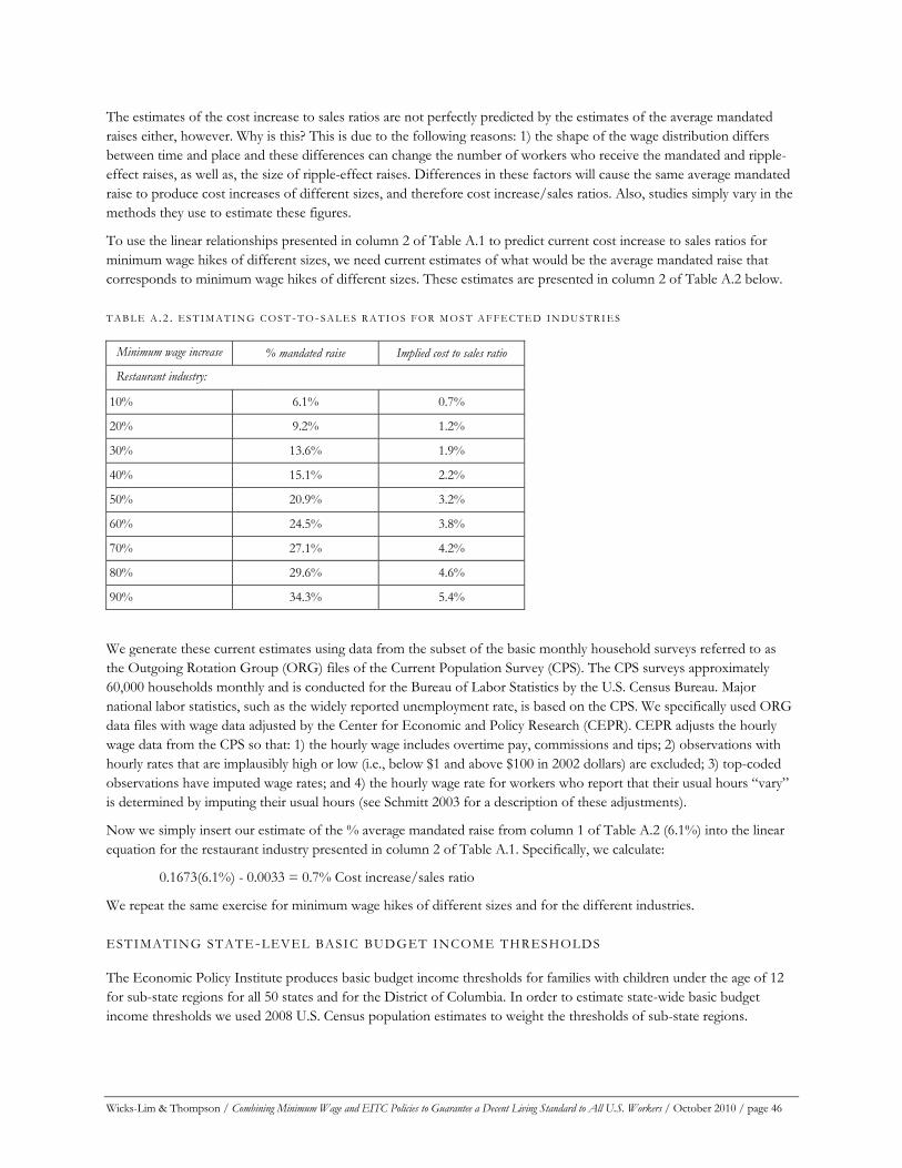
The estimates of the cost increase to sales ratios are not perfectly predicted by the estimates of the average mandated raises either, however. Why is this? This is due to the following reasons: 1) the shape of the wage distribution differs between time and place and these differences can change the number of workers who receive the mandated and ripple-effect raises, as well as, the size of ripple-effect raises. Differences in these factors will cause the same average mandated raise to produce cost increases of different sizes, and therefore cost increase/sales ratios. Also, studies simply vary in the methods they use to estimate these figures.
To use the linear relationships presented in column 2 of Table A.1 to predict current cost increase to sales ratios for minimum wage hikes of different sizes, we need current estimates of what would be the average mandated raise that corresponds to minimum wage hikes of different sizes. These estimates are presented in column 2 of Table A.2 below.
T A B L E A . 2 . E S T I M A T I N G C O S T- T O- S A L E S R A T I O S F O R M O S T A F F E C T E D I N D U S T R I E S
Minimum wage increase % mandated raise Implied cost to sales ratio
Restaurant industry: /
10% 6.1% 0.7%
20% 9.2% 1.2%
30% 13.6% 1.9%
40% 15.1% 2.2%
50% 20.9% 3.2%
60% 24.5% 3.8%
70% 27.1% 4.2%
80% 29.6% 4.6%
90% 34.3% 5.4%
We generate these current estimates using data from the subset of the basic monthly household surveys referred to as the Outgoing Rotation Group (ORG) files of the Current Population Survey (CPS). The CPS surveys approximately 60,000 households monthly and is conducted for the Bureau of Labor Statistics by the U.S. Census Bureau. Major national labor statistics, such as the widely reported unemployment rate, is based on the CPS. We specifically used ORG data files with wage data adjusted by the Center for Economic and Policy Research (CEPR). CEPR adjusts the hourly wage data from the CPS so that: 1) the hourly wage includes overtime pay, commissions and tips; 2) observations with hourly rates that are implausibly high or low (i.e., below $1 and above $100 in 2002 dollars) are excluded; 3) top-coded observations have imputed wage rates; and 4) the hourly wage rate for workers who report that their usual hours “vary” is determined by imputing their usual hours (see Schmitt 2003 for a description of these adjustments).
Now we simply insert our estimate of the % average mandated raise from column 1 of Table A.2 (6.1%) into the linear equation for the restaurant industry presented in column 2 of Table A.1. Specifically, we calculate:
0.1673(6.1%) - 0.0033 = 0.7% Cost increase/sales ratio
We repeat the same exercise for minimum wage hikes of different sizes and for the different industries.
ESTIMATING STATE-LEVEL BASIC BUDGET INCOME THRESHOLDS
The Economic Policy Institute produces basic budget income thresholds for families with children under the age of 12 for sub-state regions for all 50 states and for the District of Columbia. In order to estimate state-wide basic budget income thresholds we used 2008 U.S. Census population estimates to weight the thresholds of sub-state regions.
Wicks-Lim & Thompson / Combining Minimum Wage and EITC Policies to Guarantee a Decent Living Standard to All U.S. Workers / October 2010 / page 46
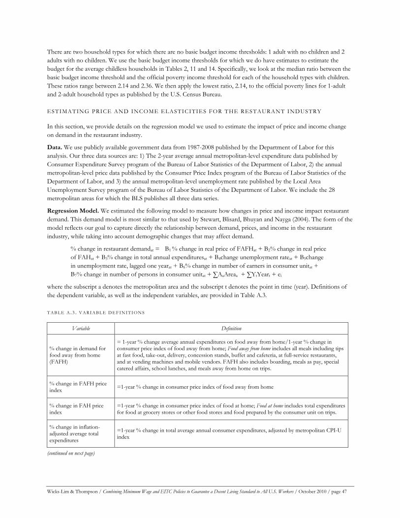
There are two household types for which there are no basic budget income thresholds: 1 adult with no children and 2 adults with no children. We use the basic budget income thresholds for which we do have estimates to estimate the budget for the average childless households in Tables 2, 11 and 14. Specifically, we look at the median ratio between the basic budget income threshold and the official poverty income threshold for each of the household types with children. These ratios range between 2.14 and 2.36. We then apply the lowest ratio, 2.14, to the official poverty lines for 1-adult and 2-adult household types as published by the U.S. Census Bureau.
ESTIMATING PRICE AND INCOME ELASTICITIES FOR THE RESTAURANT INDUSTRY
In this section, we provide details on the regression model we used to estimate the impact of price and income change on demand in the restaurant industry.
Data. We use publicly available government data from 1987-2008 published by the Department of Labor for this analysis. Our three data sources are: 1) The 2-year average annual metropolitan-level expenditure data published by Consumer Expenditure Survey program of the Bureau of Labor Statistics of the Department of Labor, 2) the annual metropolitan-level price data published by the Consumer Price Index program of the Bureau of Labor Statistics of the Department of Labor, and 3) the annual metropolitan-level unemployment rate published by the Local Area Unemployment Survey program of the Bureau of Labor Statistics of the Department of Labor. We include the 28 metropolitan areas for which the BLS publishes all three data series.
Regression Model. We estimated the following model to measure how changes in price and income impact restaurant demand. This demand model is most similar to that used by Stewart, Blisard, Bhuyan and Nayga (2004). The form of the model reflects our goal to capture directly the relationship between demand, prices, and income in the restaurant industry, while taking into account demographic changes that may affect demand.
% change in restaurant demandat = B1 % change in real price of FAFHat + B2% change in real price of FAHat + B3% change in total annual expendituresat + B4change unemployment rateat + B5change in unemployment rate, lagged one yearat + B6% change in number of earners in consumer unitat + B7% change in number of persons in consumer unitat + ∑AaAreaa + ∑YtYeart + ei
where the subscript a denotes the metropolitan area and the subscript t denotes the point in time (year). Definitions of the dependent variable, as well as the independent variables, are provided in Table A.3.
T A B L E A . 3 . V A R I A B L E D E F I N I T I O N S
Variable Definition
% change in demand for food away from home (FAFH)
= 1-year % change average annual expenditures on food away from home/1-year % change in consumer price index of food away from home; Food away from home includes all meals including tips at fast food, take-out, delivery, concession stands, buffet and cafeteria, at full-service restaurants, and at vending machines and mobile vendors. FAFH also includes boarding, meals as pay, special catered affairs, school lunches, and meals away from home on trips.
% change in FAFH price index =1-year % change in consumer price index of food away from home
% change in FAH price index
=1-year % change in consumer price index of food at home; Food at home includes total expenditures for food at grocery stores or other food stores and food prepared by the consumer unit on trips.
% change in inflation-adjusted average total expenditures
=1-year % change in total average annual consumer expenditures, adjusted by metropolitan CPI-U index
(continued on next page)
Wicks-Lim & Thompson / Combining Minimum Wage and EITC Policies to Guarantee a Decent Living Standard to All U.S. Workers / October 2010 / page 47
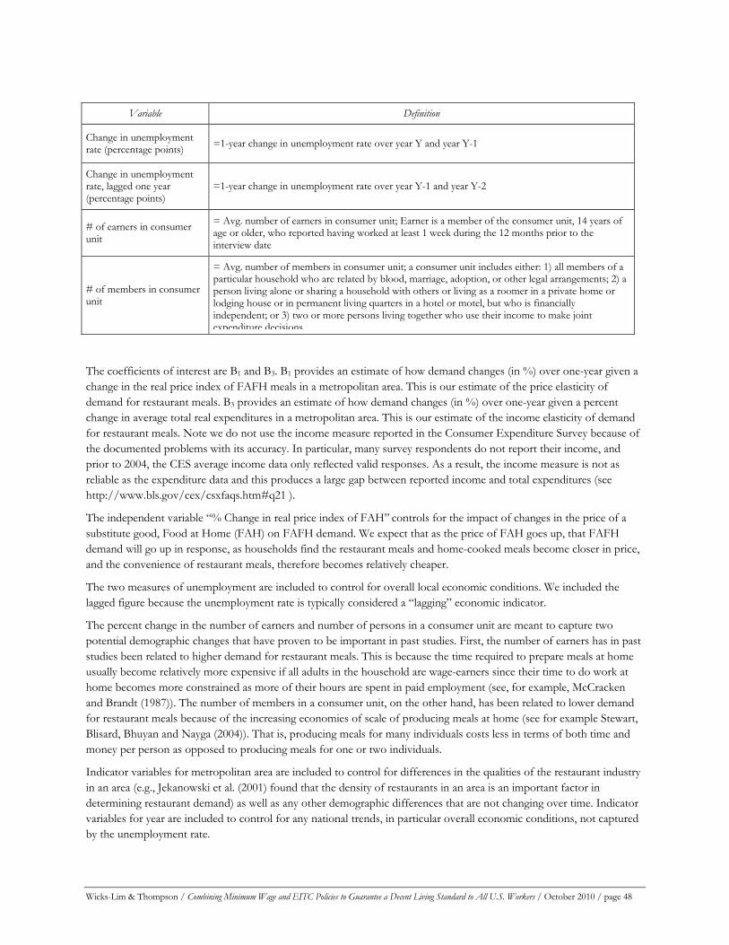
Variable Definition
Change in unemployment rate (percentage points) =1-year change in unemployment rate over year Y and year Y-1
Change in unemployment rate, lagged one year (percentage points)
=1-year change in unemployment rate over year Y-1 and year Y-2
# of earners in consumer unit
= Avg. number of earners in consumer unit; Earner is a member of the consumer unit, 14 years of age or older, who reported having worked at least 1 week during the 12 months prior to the interview date
# of members in consumer unit
= Avg. number of members in consumer unit; a consumer unit includes either: 1) all members of a particular household who are related by blood, marriage, adoption, or other legal arrangements; 2) a person living alone or sharing a household with others or living as a roomer in a private home or lodging house or in permanent living quarters in a hotel or motel, but who is financially independent; or 3) two or more persons living together who use their income to make joint expenditure decisions.
The coefficients of interest are B1 and B3. B1 provides an estimate of how demand changes (in %) over one-year given a change in the real price index of FAFH meals in a metropolitan area. This is our estimate of the price elasticity of demand for restaurant meals. B3 provides an estimate of how demand changes (in %) over one-year given a percent change in average total real expenditures in a metropolitan area. This is our estimate of the income elasticity of demand for restaurant meals. Note we do not use the income measure reported in the Consumer Expenditure Survey because of the documented problems with its accuracy. In particular, many survey respondents do not report their income, and prior to 2004, the CES average income data only reflected valid responses. As a result, the income measure is not as reliable as the expenditure data and this produces a large gap between reported income and total expenditures (see http://www.bls.gov/cex/csxfaqs.htm#q21 ).
The independent variable “% Change in real price index of FAH” controls for the impact of changes in the price of a substitute good, Food at Home (FAH) on FAFH demand. We expect that as the price of FAH goes up, that FAFH demand will go up in response, as households find the restaurant meals and home-cooked meals become closer in price, and the convenience of restaurant meals, therefore becomes relatively cheaper.
The two measures of unemployment are included to control for overall local economic conditions. We included the lagged figure because the unemployment rate is typically considered a “lagging” economic indicator.
The percent change in the number of earners and number of persons in a consumer unit are meant to capture two potential demographic changes that have proven to be important in past studies. First, the number of earners has in past studies been related to higher demand for restaurant meals. This is because the time required to prepare meals at home usually become relatively more expensive if all adults in the household are wage-earners since their time to do work at home becomes more constrained as more of their hours are spent in paid employment (see, for example, McCracken and Brandt (1987)). The number of members in a consumer unit, on the other hand, has been related to lower demand for restaurant meals because of the increasing economies of scale of producing meals at home (see for example Stewart, Blisard, Bhuyan and Nayga (2004)). That is, producing meals for many individuals costs less in terms of both time and money per person as opposed to producing meals for one or two individuals.
Indicator variables for metropolitan area are included to control for differences in the qualities of the restaurant industry in an area (e.g., Jekanowski et al. (2001) found that the density of restaurants in an area is an important factor in determining restaurant demand) as well as any other demographic differences that are not changing over time. Indicator variables for year are included to control for any national trends, in particular overall economic conditions, not captured by the unemployment rate.
Wicks-Lim & Thompson / Combining Minimum Wage and EITC Policies to Guarantee a Decent Living Standard to All U.S. Workers / October 2010 / page 48
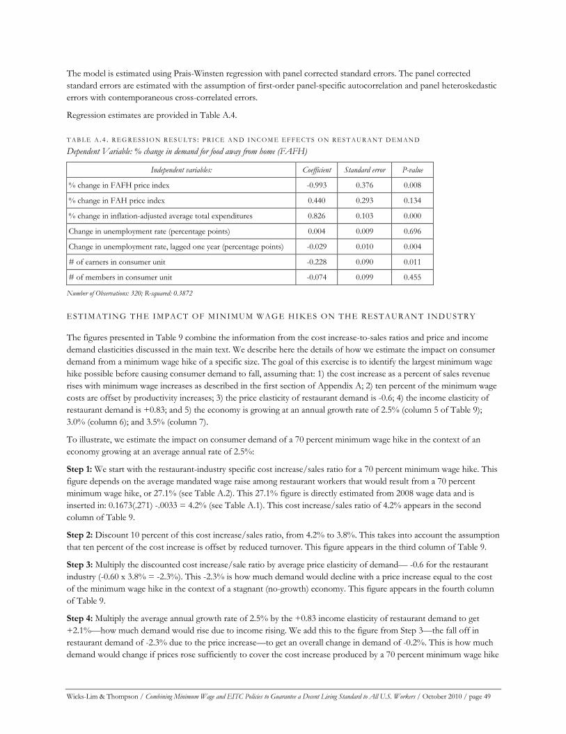
The model is estimated using Prais-Winsten regression with panel corrected standard errors. The panel corrected standard errors are estimated with the assumption of first-order panel-specific autocorrelation and panel heteroskedastic errors with contemporaneous cross-correlated errors.
Regression estimates are provided in Table A.4.
T A B L E A . 4 . R E G R E S S I O N R E S U L T S : P R I C E A N D I N C O M E E F F E C T S O N R E S T A U R A N T D E M A N D Dependent Variable: % change in demand for food away from home (FAFH)
Independent variables: Coefficient Standard error P-value
% change in FAFH price index -0.993 0.376 0.008
% change in FAH price index 0.440 0.293 0.134
% change in inflation-adjusted average total expenditures 0.826 0.103 0.000
Change in unemployment rate (percentage points) 0.004 0.009 0.696
Change in unemployment rate, lagged one year (percentage points) -0.029 0.010 0.004
# of earners in consumer unit -0.228 0.090 0.011
# of members in consumer unit -0.074 0.099 0.455
Number of Observations: 320; R-squared: 0.3872
ESTIMATING THE IMPACT OF MINIMUM WAGE HIKES ON THE RESTAURANT INDUSTRY
The figures presented in Table 9 combine the information from the cost increase-to-sales ratios and price and income demand elasticities discussed in the main text. We describe here the details of how we estimate the impact on consumer demand from a minimum wage hike of a specific size. The goal of this exercise is to identify the largest minimum wage hike possible before causing consumer demand to fall, assuming that: 1) the cost increase as a percent of sales revenue rises with minimum wage increases as described in the first section of Appendix A; 2) ten percent of the minimum wage costs are offset by productivity increases; 3) the price elasticity of restaurant demand is -0.6; 4) the income elasticity of restaurant demand is +0.83; and 5) the economy is growing at an annual growth rate of 2.5% (column 5 of Table 9); 3.0% (column 6); and 3.5% (column 7).
To illustrate, we estimate the impact on consumer demand of a 70 percent minimum wage hike in the context of an economy growing at an average annual rate of 2.5%:
Step 1: We start with the restaurant-industry specific cost increase/sales ratio for a 70 percent minimum wage hike. This figure depends on the average mandated wage raise among restaurant workers that would result from a 70 percent minimum wage hike, or 27.1% (see Table A.2). This 27.1% figure is directly estimated from 2008 wage data and is inserted in: 0.1673(.271) -.0033 = 4.2% (see Table A.1). This cost increase/sales ratio of 4.2% appears in the second column of Table 9.
Step 2: Discount 10 percent of this cost increase/sales ratio, from 4.2% to 3.8%. This takes into account the assumption that ten percent of the cost increase is offset by reduced turnover. This figure appears in the third column of Table 9.
Step 3: Multiply the discounted cost increase/sale ratio by average price elasticity of demand— -0.6 for the restaurant industry (-0.60 x 3.8% = -2.3%). This -2.3% is how much demand would decline with a price increase equal to the cost of the minimum wage hike in the context of a stagnant (no-growth) economy. This figure appears in the fourth column of Table 9.
Step 4: Multiply the average annual growth rate of 2.5% by the +0.83 income elasticity of restaurant demand to get +2.1%—how much demand would rise due to income rising. We add this to the figure from Step 3—the fall off in restaurant demand of -2.3% due to the price increase—to get an overall change in demand of -0.2%. This is how much demand would change if prices rose sufficiently to cover the cost increase produced by a 70 percent minimum wage hike
Wicks-Lim & Thompson / Combining Minimum Wage and EITC Policies to Guarantee a Decent Living Standard to All U.S. Workers / October 2010 / page 49

in the context of a growing economy. This is the figure in the fifth column.
These four steps can be written as the following formula:
Change in restaurant demand = (-0.6 )(0.9)[C(Avg. Mandated Raise from X% Min. Wage Increase)] + (+0.83) (Annual Growth Rate of the U.S. Economy)
where the average mandated wage raise from a minimum wage hike of X percent is directly estimated from 2008 wage data and presented in Table A.2. The “cost” function that determines the % cost increase relative to sales revenue among restaurants given an average mandated raise is defined in Table A.1. We determine the largest minimum hike possible before causing consumer demand to fall by identifying the minimum wage hike for which demand changes from positive to negative.
ESTIMATING IMPACT OF 70% MINIMUM WAGE HIKE ON OTHER INDUSTRIES
The impact of a 70% minimum wage hike for other industries is estimated in the same way as for the restaurant industry. The only difference is that industry specific elasticities are used. See Table A.5 for industry-specific price elasticities of demand. See Table A.6 for industry-specific income elasticities of demand.
T A B L E A . 5 . I M P A C T O F 1 % P R I C E I N C R E A S E O N C O N S U M E R D E M A N D B Y I N D U S T R Y
% change in consumer demand due to 1% price increase Industry
Range of estimates Average
Hotels
• Canina et al. (2005): -0.13% • Hiemstra and Ismail (1992): -0.44% • Wheaton and Rossoff (1996): -0.48% • Coopers and Lybrand : -0.40%
-0.13% to -0.48% -0.4%
Administrative & support, waste management & remediation services • Falvey and Gemmell (1996; used government services): -1.3%
(average of -1.2% and -1.4%) -1.3% -1.3%
Health services • Falvey and Gemmell (1996): -0.8% • Wang (2009): less than -1.0% • From literature review in Rechovsky (1998): -0.16% to -2.3% • Reschovsky (1996): -1.0%.
-0.16% to -2.3% -1.0%
Arts, entertainment and recreation • Nelson (2001): -0.88% • Falvey and Gemmell (1996): -1.3% (average of -1.0% and -1.6%); • Felton (1992): -0.54% (average of -0.13% and -0.95%).
-0.13% to -1.3% -0.9%
Other services (e.g., repair, laundry, and private household services) • Falvey and Gemmel (1996; used other household goods and
services): -1.3% (average of -1.2% and -1.3%) • Moller (2001): -0.3%
-0.3% to -1.3% -0.8%
Retail trade • Moller (2001): -0.63% • Nelson (2001): -0.71% • Falvey and Gemmel (1996; other household goods and services): -
1.3% (average of -1.2% to -1.3%) • Moktari (1992): -1.5% (average of -1.0% and -1.9%) • Richards et al. (2006): -1.0% • Piggott (2003): -0.50% (average of -0.44% to -0.54%) • Park et al. (1996): -0.4% (average of -0.1% to -0.6%)
-0.4% to -1.9% -0.9%
(continued on next page)
Wicks-Lim & Thompson / Combining Minimum Wage and EITC Policies to Guarantee a Decent Living Standard to All U.S. Workers / October 2010 / page 50
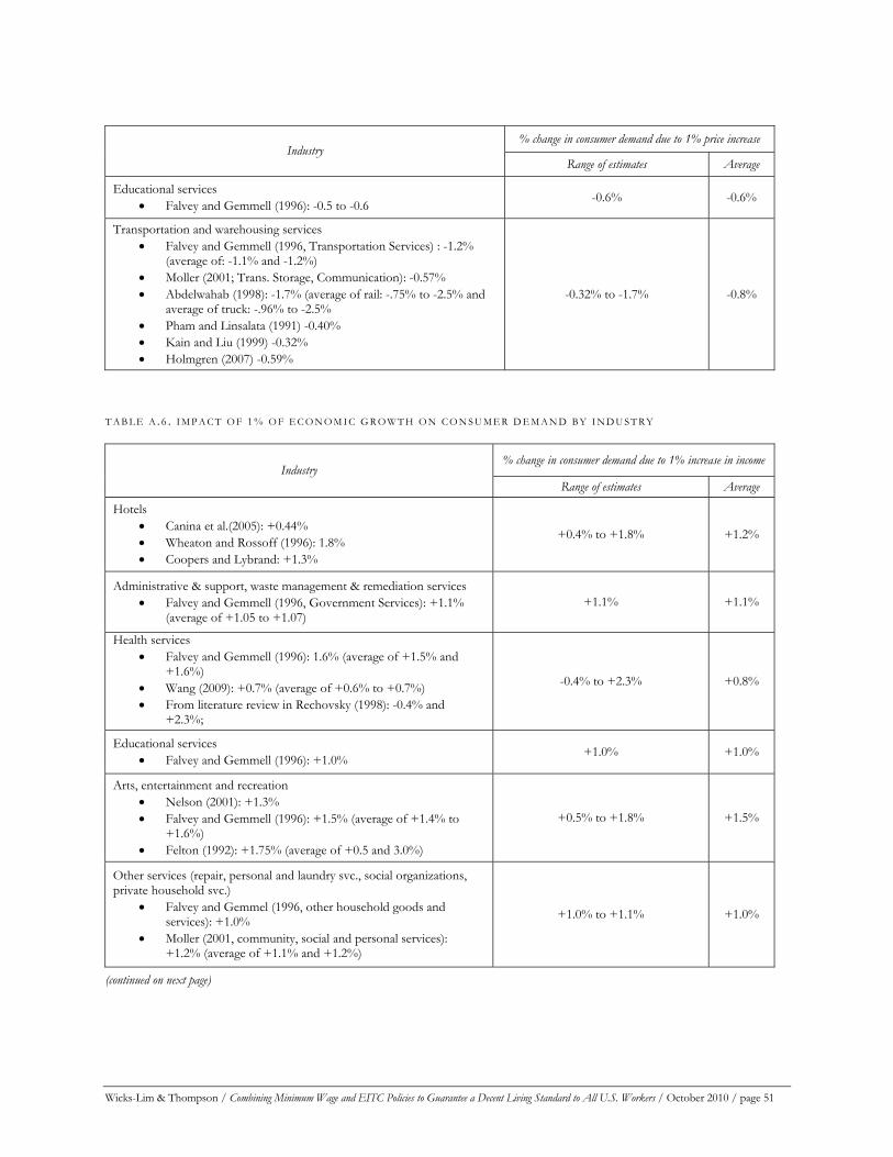
% change in consumer demand due to 1% price increase
Industry Range of estimates Average
Educational services
• Falvey and Gemmell (1996): -0.5 to -0.6 -0.6% -0.6%
Transportation and warehousing services • Falvey and Gemmell (1996, Transportation Services) : -1.2%
(average of: -1.1% and -1.2%) • Moller (2001; Trans. Storage, Communication): -0.57% • Abdelwahab (1998): -1.7% (average of rail: -.75% to -2.5% and
average of truck: -.96% to -2.5% • Pham and Linsalata (1991) -0.40% • Kain and Liu (1999) -0.32% • Holmgren (2007) -0.59%
-0.32% to -1.7% -0.8%
T A B L E A . 6 . I M P A C T O F 1 % O F E C O N O M I C G R O W T H O N C O N S U M E R D E M A N D B Y I N D U S T R Y
% change in consumer demand due to 1% increase in income Industry
Range of estimates Average
Hotels • Canina et al.(2005): +0.44% • Wheaton and Rossoff (1996): 1.8% • Coopers and Lybrand: +1.3%
+0.4% to +1.8% +1.2%
Administrative & support, waste management & remediation services • Falvey and Gemmell (1996, Government Services): +1.1%
(average of +1.05 to +1.07) +1.1% +1.1%
Health services • Falvey and Gemmell (1996): 1.6% (average of +1.5% and
+1.6%) • Wang (2009): +0.7% (average of +0.6% to +0.7%) • From literature review in Rechovsky (1998): -0.4% and
+2.3%;
-0.4% to +2.3% +0.8%
Educational services
• Falvey and Gemmell (1996): +1.0% +1.0% +1.0%
Arts, entertainment and recreation • Nelson (2001): +1.3% • Falvey and Gemmell (1996): +1.5% (average of +1.4% to
+1.6%) • Felton (1992): +1.75% (average of +0.5 and 3.0%)
+0.5% to +1.8% +1.5%
Other services (repair, personal and laundry svc., social organizations, private household svc.)
• Falvey and Gemmel (1996, other household goods and services): +1.0%
• Moller (2001, community, social and personal services): +1.2% (average of +1.1% and +1.2%)
+1.0% to +1.1% +1.0%
(continued on next page)
Wicks-Lim & Thompson / Combining Minimum Wage and EITC Policies to Guarantee a Decent Living Standard to All U.S. Workers / October 2010 / page 51
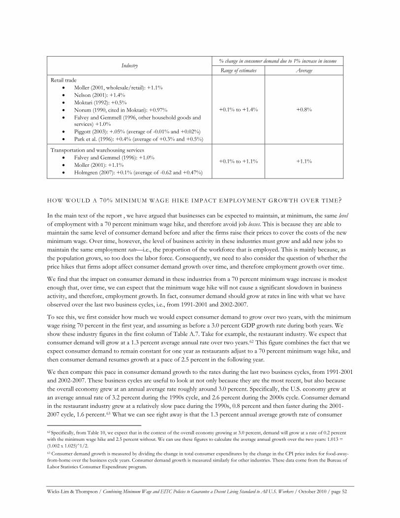
Wicks-Lim & Thompson / Combining Minimum Wage and EITC Policies to Guarantee a Decent Living Standard to All U.S. Workers / October 2010 / page 52
% change in consumer demand due to 1% increase in income
Industry Range of estimates Average
Retail trade • Moller (2001, wholesale/retail): +1.1% • Nelson (2001): +1.4% • Moktari (1992): +0.5% • Norum (1990, cited in Moktari): +0.97% • Falvey and Gemmell (1996, other household goods and
services) +1.0% • Piggott (2003): +.05% (average of -0.01% and +0.02%) • Park et al. (1996): +0.4% (average of +0.3% and +0.5%)
+0.1% to +1.4% +0.8%
Transportation and warehousing services • Falvey and Gemmel (1996): +1.0% • Moller (2001): +1.1% • Holmgren (2007): +0.1% (average of -0.62 and +0.47%)
+0.1% to +1.1% +1.1%
HOW WOULD A 70% MINIMUM WAGE HIKE IMPACT EMPLOYMENT GROWTH OVER TIME?
In the main text of the report , we have argued that businesses can be expected to maintain, at minimum, the same level of employment with a 70 percent minimum wage hike, and therefore avoid job losses. This is because they are able to maintain the same level of consumer demand before and after the firms raise their prices to cover the costs of the new minimum wage. Over time, however, the level of business activity in these industries must grow and add new jobs to maintain the same employment rate—i.e., the proportion of the workforce that is employed. This is mainly because, as the population grows, so too does the labor force. Consequently, we need to also consider the question of whether the price hikes that firms adopt affect consumer demand growth over time, and therefore employment growth over time.
We find that the impact on consumer demand in these industries from a 70 percent minimum wage increase is modest enough that, over time, we can expect that the minimum wage hike will not cause a significant slowdown in business activity, and therefore, employment growth. In fact, consumer demand should grow at rates in line with what we have observed over the last two business cycles, i.e., from 1991-2001 and 2002-2007.
To see this, we first consider how much we would expect consumer demand to grow over two years, with the minimum wage rising 70 percent in the first year, and assuming as before a 3.0 percent GDP growth rate during both years. We show these industry figures in the first column of Table A.7. Take for example, the restaurant industry. We expect that consumer demand will grow at a 1.3 percent average annual rate over two years.62 This figure combines the fact that we expect consumer demand to remain constant for one year as restaurants adjust to a 70 percent minimum wage hike, and then consumer demand resumes growth at a pace of 2.5 percent in the following year.
We then compare this pace in consumer demand growth to the rates during the last two business cycles, from 1991-2001 and 2002-2007. These business cycles are useful to look at not only because they are the most recent, but also because the overall economy grew at an annual average rate roughly around 3.0 percent. Specifically, the U.S. economy grew at an average annual rate of 3.2 percent during the 1990s cycle, and 2.6 percent during the 2000s cycle. Consumer demand in the restaurant industry grew at a relatively slow pace during the 1990s, 0.8 percent and then faster during the 2001-2007 cycle, 1.6 percent.63 What we can see right away is that the 1.3 percent annual average growth rate of consumer
62 Specifically, from Table 10, we expect that in the context of the overall economy growing at 3.0 percent, demand will grow at a rate of 0.2 percent with the minimum wage hike and 2.5 percent without. We can use these figures to calculate the average annual growth over the two years: 1.013 = (1.002 x 1.025)^1/2. 63 Consumer demand growth is measured by dividing the change in total consumer expenditures by the change in the CPI price index for food-away-from-home over the business cycle years. Consumer demand growth is measured similarly for other industries. These data come from the Bureau of Labor Statistics Consumer Expenditure program.
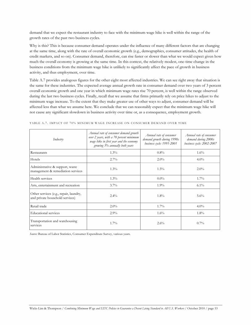
demand that we expect the restaurant industry to face with the minimum wage hike is well within the range of the growth rates of the past two business cycles.
Why is this? This is because consumer demand operates under the influence of many different factors that are changing at the same time, along with the rate of overall economic growth (e.g., demographics, consumer attitudes, the health of credit markets, and so on). Consumer demand, therefore, can rise faster or slower than what we would expect given how much the overall economy is growing at the same time. In this context, the relatively modest, one-time change in the business conditions from the minimum wage hike is unlikely to significantly affect the pace of growth in business activity, and thus employment, over time.
Table A.7 provides analogous figures for the other eight most affected industries. We can see right away that situation is the same for these industries. The expected average annual growth rate in consumer demand over two years of 3 percent overall economic growth and one year in which minimum wage rates rise 70 percent, is well within the range observed during the last two business cycles. Finally, recall that we assume that firms primarily rely on price hikes to adjust to the minimum wage increase. To the extent that they make greater use of other ways to adjust, consumer demand will be affected less than what we assume here. We conclude that we can reasonably expect that the minimum wage hike will not cause any significant slowdown in business activity over time or, as a consequence, employment growth.
T A B L E A . 7 . I M P A C T O F 7 0 % M I N I M U M W A G E I N C R E A S E O N C O N S U M E R D E M A N D O V E R T I M E
Industry
Annual rate of consumer demand growth over 2 years, with a 70 percent minimum wage hike in first year and the economy
growing 3% annually both years
Annual rate of consumer demand growth during 1990s
business cycle: 1991-2001
Annual rate of consumer demand during 2000s
business cycle: 2002-2007
Restaurants 1.3% 0.8% 1.6%
Hotels 2.7% 2.0% 4.0%
Administrative & support, waste management & remediation services 1.3% 1.5% 2.0%
Health services 1.3% 0.0% 1.7%
Arts, entertainment and recreation 3.7% 1.9% 6.1%
Other services (e.g., repair, laundry, and private household services) 2.4% 1.8% 5.6%
Retail trade 2.0% 1.7% 4.0%
Educational services 2.9% 1.6% 1.8%
Transportation and warehousing services 1.7% 2.6% 0.7%
Source: Bureau of Labor Statistics, Consumer Expenditure Survey, various years.
Wicks-Lim & Thompson / Combining Minimum Wage and EITC Policies to Guarantee a Decent Living Standard to All U.S. Workers / October 2010 / page 53
Appendix B: Details on Estimating EITC Expansion Costs
Changes in the number of EITC recipients, the total benefits, and later the costs of the expansions are developed by modeling the program rules using the Current Population Survey. As a baseline, the current policy, including the maximum benefit level and the different portions of the benefit schedule is replicated. Changes to those parameters, specifically raising the earnings level where the phase-in, plateau, and phase-out portions of the benefit schedule end, will result in additional households being eligible for credit. The number of eligible households and the benefits they receive are adjusted with sampling weights in the CPS, and changes in total benefits and recipient households are used to reflect the impact and cost of the different expansion scenarios. The impact of the minimum wage change is modeled by altering the earnings of individual workers with wages below the proposed minimum. These modified earnings figures are combined with other income to determine eligibility and benefit amounts under the current and the proposed expansions to the EITC.
DATA
The March Supplement to the Current Population Survey is a nationally representative survey that reaches 50,000 households each year, and contains sufficient demographic, employment, and income data to model the EITC policy rules. Data from 2005, 2006, and 2007 are used, chosen because they are among the most current data available and also do not include the effects of the 2008-2009 recession. Data for 2009 were not available at the time of this analysis, and data for 2008 were not included. With such high rates of unemployment in 2008 and 2009, cost estimates of a program for working families would appear lower than what we might expect in a typical year.
MINIMUM WAGE
A minimum wage level of $12.30 (in 2009 dollars) is used in the expansion scenario. The nominal values of the minimum wage were adjusted for inflation back to constant levels for 2005, 2007, and 2007. The fifteen states with minimum wages above the federal level were given higher minima in the modeled expansion scenario. The minimum wage rates for these states were obtained by simply multiplying the 2009 percentage premium over the federal level by inflation-adjusted level of the new federal minimum.
To model the impacts of a change in the minimum wage on the earnings and incomes of workers in the CPS, we first need to identify those workers who currently are paid at rates below the proposed new minimum wage. The March supplement, however, lacks the same detailed variables on hourly earnings and hours worked that are present in the standard outgoing rotation group (ORG) data. The March supplement contains information on annual earnings, usual hours worked per week, and weeks worked in the prior year. These variables can be used to construct a measure of hourly wages. Because of variation in hours worked across a year and problems with accurate recall, this constructed measure of wages is not as reliable as the one in the ORG data, which directly measures the hourly wage and reflects information on hours worked in the previous week.
We can, however, use the wage data for the quarter of the March sample in the ORG months, and use a matching procedure to obtain wage data for many of the remaining workers. Households that are in the CPS sample appear in the survey for four consecutive months, are left out of the sample for eight months, and are then surveyed again for four consecutive months before being dropped permanently from the sample. Of their eight total potential months in the sample, households are asked detailed wage and labor force questions in the fourth and eighth months, referred to the outgoing rotation groups. Each March, when the demographic and income supplement is conducted, one quarter of the sample are in the ORG month and are asked the wage and labor force questions.
The remaining three quarters of the sample are in an ORG month over the following three months. For those households, we use CPS household and individual identifiers to link to the wage data for those individuals contained in the April, May and June surveys. This same matching procedure is used by researchers at the Urban Institute with their
Wicks-Lim & Thompson / Combining Minimum Wage and EITC Policies to Guarantee a Decent Living Standard to All U.S. Workers / October 2010 / page 54
Wicks-Lim & Thompson / Combining Minimum Wage and EITC Policies to Guarantee a Decent Living Standard to All U.S. Workers / October 2010 / page 55
TRIM3 model, and is described in detail in Madrian and Lefgren (2000).64
We are able to obtain ORG wage data for seventy-six percent of the working people in the March surveys for 2005-2007. Fifty-four percent are directly-measured hourly wages for workers paid hourly and 22 percent are wages for workers not paid hourly and are calculated by dividing weekly wages by hours worked. Reasons why some observations with positive annual earnings in the March survey cannot be linked to useable hourly wage data from ORG months succeeding months include: 1) attrition, as some households cannot be located or move during the survey period, 2) change in the composition of the household, as some members move away or die, 3) not being employed at the time of the ORG month survey, and 4) coding errors and irregularities that make it difficult to accurately match an individual within a household to the same observation in a different month.
For the remaining quarter of workers who cannot be linked to their ORG wage data, wages are calculated using the annual earnings, weeks, and hours from the March Supplement described above. Observations with implied hourly wages under one dollar were dropped from the sample.
EITC – MODELING BENEFITS AND FILERS
Our first step in modeling the expansion in the EITC using the CPS data is to try to replicate the existing program. Using the current program rules and sampling weights we identify the number of EITC eligible households and the total implied benefits, and compare that to the actual filers and benefit figures published by the IRS. The relevant parameters to consider are family income, earnings, and the numbers and ages of children.
INCOME AND EARNINGS
A household must have earnings from work in the tax year to be eligible for the credit, and is ineligible for the credit if they have more than a small amount of income from investments ($2,950 in 2008). In addition to the number of children in the household, the primary determinant of the amount of the credit is earnings. Earnings between $12,570 and $16,420 make a family with two young children potentially eligible for the maximum credit, but the actual credit amount also depends on other forms of income. Alimony received, for example, does not increase the credit for families with earnings below the $12,570 starting point of the benefit plateau, but does reduce the credit if it pushes adjusted gross income beyond the $16,420 end of the benefit plateau. So, earnings and income together are jointly considered when imputing an EITC benefit level to a household.
NUMBER OF CHILDREN
In 2008, the program year modeled here, there EITC credit depends on whether a household has no children, one child, or two or more children. Eligible children can only be claimed on one tax return, but they can be connected to the filer in a number of ways, as child, grandchild, niece/nephew, or in a guardianship relationship. To be eligible to be counted as a dependent child for the purposes of the EITC, a child must be under the age of 24, and any children between 19 and 23 must be full-time students to count as dependent children.
RELEVANT UNIT – FAMILIES VERSUS TAX-FILING UNITS
The EITC is actually determined by tax returns, so the most appropriate unit is the tax filing unit. The CPS, however, is a survey of households, not tax-filing units. A household is a physical place that can hold between one single person and a number of complete families, while a tax-filing unit is simply the group of people represented or “claimed” in some way on a federal income tax return. And while the CPS does provide quite detailed information on family structure and family relationships – families are two or more people related by blood or marriage – these are not the same as tax filing units. In some cases the relationship between family and tax filing unit is quite clear. Assuming, for example, that a
64 Details on use of matching in TRIM3 are described in Giannarelli et al (2007): www.urban.org/publications/411450.html.
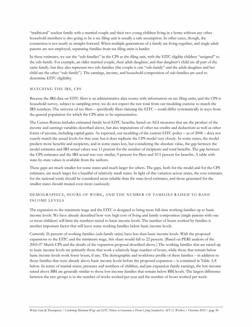
“traditional” nuclear family with a married couple and their two young children living in a home without any other household members is also going to be a tax filing unit is usually a safe assumption. In other cases, though, the connection is not nearly as straight-forward. When multiple generations of a family are living together, and single adult parents are not employed, separating families from tax filing units is harder.
In these estimates, we use the “sub-families” in the CPS as the filing unit, with the EITC eligible children “assigned” to the sub-family. For example, an older married couple, their adult daughter, and that daughter’s child are all part of the same family, but they also represent two sub-families (the couple is one “sub-family” and the adult daughter and her child are the other “sub-family”). The earnings, income, and household composition of sub-families are used to determine EITC eligibility.
MATCHING THE IRS, CPS
Because the IRS data on EITC filers is an administrative data source with information on tax filing units, and the CPS is household survey, subject to sampling error, we do not expect the raw total from our modeling exercise to match the IRS numbers. The universe of tax filers – specifically filers claiming the EITC – could differ systematically in ways from the general population for which the CPS aims to be representative.
The Census Bureau includes estimated family level EITC benefits, based on AGI measures that are the product of the income and earnings variables described above, but also imputations of other tax credits and deductions as well as other forms of income, including capital gains. As expected, our modeling of the current EITC policy – as of 2008 – does not exactly match the actual levels for that year, but it does replicate the CPS model very closely. In some states, the model predicts more benefits and recipients, and in some states less, but considering the absolute value, the gap between the model estimates and IRS actual values was 11 percent for the number of recipients and total benefits. The gap between the CPS estimates and the IRS actual was very similar, 9 percent for filers and 10.5 percent for benefits. A table with state-by-state values is available from the authors.
These gaps are much smaller for some states and much larger for others. The gaps, both for the model and for the CPS estimates, are much larger for a handful of relatively small states. In light of this variation across states, the cost estimates for the national totals should be considered more reliable than the state-level estimates, and those generated for the smaller states should treated even more cautiously.
DEMOGRAPHICS, HOURS OF WORK, AND THE NUMBER OF FAMILIES RAISED TO BASIC INCOME LEVELS
The expansion to the minimum wage and the EITC is designed to bring most full-time working families up to basic income levels. We have already described how very high cost of living and family composition (single parents with one or more children) will limit the numbers raised to basic income levels. The number of hours worked by families is another important factor that will leave some working families below basic income levels.
Currently 26 percent of working families (sub-family units) have less than basic income levels. With the proposed expansions to the EITC and the minimum wage, this share would fall to 22 percent. (Based on PERI analysis of the 2005-07 March CPS and the details of the expansion proposal described above.) The working families that are raised up to basic income levels are primarily those that work a relatively large number of hours, while those that remain below basic income levels work fewer hours, if any. The demographic and workforce profile of these families – in addition to those families that were already above basic income levels before the proposed expansion – is contained in Table A.8 below. In terms of marital status, presence and numbers of children, and pre-expansion family earnings, the low-income raised above BBI are generally similar to those low-income families that remain below BBI levels. The largest difference between the two groups is in the number of weeks worked per year and the number of hours worked per week.
Wicks-Lim & Thompson / Combining Minimum Wage and EITC Policies to Guarantee a Decent Living Standard to All U.S. Workers / October 2010 / page 56
T A B L E A .8 . D E M O G R A P H I C A N D W O R K F O R C E P R O F I L E O F W O R K I N G H O U S E H O L D S , B Y L O W- I N C O M E S T A T U S
B E F O R E A N D A F T E R M I N I M U M W A G E I N C R E A S E A N D E I T C E X P A N S I O N
Low-income working households before expansion
Raised above basic budget
income threshold by MW and EITC increases
Remaining below basic budget income threshold by MW and
EITC increases
Already above basic budget income threshold before by MW and EITC increases
Share of low-income working families 16% 84% -
Average # of children 0.75 0.79 0.52 % with one child 23% 20% 15% % with 2+ children 26% 29% 18% % with any children 49% 50% 34% % married 41% 34% 63% Average hours worked per year 1,831 1,291 1,874 Average hours per week 37.2 30.2 37.6 Average weeks per year 44.5 36.0 44.4 % working full-year, full- time 73.3% 31.2% 73% % working full-time 79.7% 42.7% 78% % working full year 78.0% 39.4% 77%
Average family earnings before expansion $21,371 $11,280 $72,733
Source: PERI analysis of March CPS (2005 to 2007) and expansion proposal details.
Wicks-Lim & Thompson / Combining Minimum Wage and EITC Policies to Guarantee a Decent Living Standard to All U.S. Workers / October 2010 / page 57
REFERENCES
Aaronson, Daniel, Eric French, and James MacDonald. 2005. “The Minimum Wage, Restaurant Prices, and Labor Market Structure.” Federal Reserve of Chicago Working Paper No. 2004-21.
Abdelwahab, Walid M. 1998. “Elasticities of Mode Choice Probabilities and Market Elasticities of Demand: Evidence from a Simultaneous Mode Choice/Shipment-Size Freight Transport Model.” Transportation Research Part E: Logistics and Transportation Review 34 (4): 257-66.
Akerlof, George and Janet Yellen. 1986. Efficiency Wage Models of the Labor Market. New York: Cambridge University Press.
Baker, Dean, Robert Pollin, Travis McArthur, and Matt Sherman (2009), “The Potential Revenue from Financial Transactions Taxes,” PERI – CEPR Working Paper, December 2009, available at: http://www.peri.umass.edu/236/hash/7cd9f46fbb/publication/393/.
Bewley, Truman F. 1999. Why Wages Don’t Fall During a Recession. Cambridge, MA: Harvard University Press.
Bluestone, Barry and Teresa Ghilaraducci. 1996. “Making Work Pay.” Public Policy Brief No.28, Jerome Levy Economics Institute of Bard College, Annadale-on-Hudson, NY: Levy Institute.
Boushey, Heather, Chauna Brocht, Bethney Gundersen, and Jared Bernstein. 2001. Hardships in America: The Real Story of Working Families. Washington, D.C.: Economic Policy Institute.
Bowles, Samuel. 1985. “The Production Process in a Competitive Economy: Walrasian, Neo-Hobbesian, and Marxian Models.” American Economic Review, 75 (1): 16-36.
Brenner, Mark and Stephanie Luce. 2005. Living Wage Laws in Practice: The Boston, New Haven, and Hartford Experiences. Amherst, MA: Political Economy Research Institute.
Brown, Douglas M. 1990. “The Restaurant and Fast Food Race: Who’s Winning?” Southern Economic Journal 56 (4): 969-83.
Canina, Linda, and Steven Carvell. 2005. “Lodging Demand for Urban Hotels in Major Metropolitan Markets.” Journal of Hospitality and Tourism Research 29 (3): 291-311.
Card, David, and Alan B. Krueger. 1995. Myth and Measurement: The New Economics of the Minimum Wage. Princeton, NJ: Princeton University Press.
Citro, Constance F., and Robert T. Michael, eds. 1995. Measuring Poverty: A New Approach. Washington, D.C.: National Academy Press.
Doucouliagos, Hristos, and T. D. Stanley. 2009. “Publication Selection Bias in Minimum-Wage Research? A Meta-Regression Analysis.” British Journal of Industrial Relations 47 (2): 406-28.
Dube, Arindrajit, T. William Lester, and Michael Reich. 2007. “Minimum Wage Effects Across State Borders: Estimates Using Contiguous Counties.” Institute for Research on Labor and Employment Working Paper Series No. iirwps-157-07.
Dube, Arindrajit, Suresh Naidu, and Michael Reich. 2007. “The Economic Effects of a Citywide Minimum Wage.” Industrial and Labor Relations Review 60 (4): 522-43.
Eissa, Nada and Jeffery B. Liebman. 1996. Labor Supply Response to the Earned Income Tax Credit. The Quarterly Journal of Economics, Vol. 111, (2,May), 605-637.
Eissa, Nada and Hilary Hoynes. 2004. “Taxes and the Labor Market Participation of Married Couples: the Earned Income Tax Credit,” Journal of Public Economics, Vol. 88, 1931-58.
Wicks-Lim & Thompson / Combining Minimum Wage and EITC Policies to Guarantee a Decent Living Standard to All U.S. Workers / October 2010 / page 58

——- . 2006. Behavioral Responses to Taxes: Lessons from the EITC and Labor Supply. In: J. Poterba, Editor, Tax Policy and the Economy (20th ed.), Cambridge, MA: National Bureau of Economic Research: MIT Press. pp. 74-110.
Falvey, Rodney. E., and Norman Gemmell. 1996. “Are Services Income-Elastic? Some New Evidence.” Review of Income and Wealth 42 (3): 257-69.
Fairris, David and Luis Fernandez Bujanda. 2008. “The Dissipation of Minimum Wage Gains for Workers through Labor-Labor Substitution: Evidence from the Los Angeles Living Wage Ordinance.” Southern Economic Journal Journal, 75(2): 473-496.
Fairris, David, David Runsten, Carolina Briones, and Jessica Goodheart. 2005. Examining the Evidence: The Impact of the Los Angeles Living Wage Ordinance on Workers and Businesses. Los Angeles Living Wage Study.
Felton, Marianne Victorius. 1992. “On the Assumed Inelasticity of Demand for the Performing Arts.” Journal of Cultural Economics 16 (1): 1-12.
Folbre, Nancy. 2002. The Invisible Heart: Economics and Family Values. The New Press.
Giannarelli, Linda, Joyce Morton and Laura Wheaton. 2007. “Estimating the Anti-poverty Effects of Changes in Taxes and Benefits with the TRIM3 Microsimulation Model,” Urban Institute Technical Report, April 2007.
Grogger, Jeffrey. 2003. “The Effects of Time Limits, the EITC, and Other Policy Changes on Welfare Use, Work, and Income Among Female-Headed Families,” The Review of Economics and Statistics, Vol. 83, No. 2, 394-408.
Freeman, Richard. 1995. “What will a 10%…50%…100% increase in the minimum wage do?” Industrial and Labor Relations Review 48(4), 830-834.
Hiemstra, Stephen J., and Joseph A. Ismail. 1992. “Occupancy Taxes: No Free Lunch.” Cornell Hotel and Restaurant Administration Quarterly 33 (5): 84-9.
Holmgren, Johan. 2007. “Meta-analysis of Public Transport Demand.” Transportation Research Part A: Policy and Practice 41: 1021-35.
Holt, Steve. 2006. The Earned Income Tax Credit at Age 30: What We Know. Washington, DC: The Brookings Institution.
Hotz, Joseph V., John Karl Scholz. 2003. The Earned Income Tax Credit. In: Moffitt, Robert (Ed.) Means-Tested Transfer Programs in the United States. Chicago: University of Chicago Press, 141-97.
Jekanowski, Mark D., James K. Binkley, and James Eales. 2001. “Convenience, Accessibility, and the Demand for Fast Food.” Journal of Agricultural and Resource Economics 26 (1): 58-74.
Kain, John F., and Zvi Liu. 1999. “Secrets of Success: Assessing the Large Increases in Transit Ridership Achieved by Houston and San Diego Transit Providers.” Transportation Research Part A: Policy and Practice 33 (7-8): 601-24.
Kelley, Thomas J. and Nicholas M. Kiefer, and Kenneth Burdett. 1994. “A Demand-Based Approach to Menu Pricing,” Cornell Hotel and Restaurant Administration Quarterly, 35 (1) : 48-52.
Lee, Chinkook, Gerald Schluter, and Brian O'Roark. 2000. “How Much Would Increasing the Minimum Wage Affect Food Prices?” Agricultural Information Bulletin No. 747-03.
Leigh, Andrew. 2010. “Who Benefits from the Earned Income Tax Credit? Incidence Among Recipients, Coworkers, and Firms” BE Journal of Economic Analysis & Policy, Vol. 10, No. 1, Article 45.
Levitas, Jason A. and Nicholas Johnson. 2006. Together, State Minimum Wages and State Earned Income Tax Credits Make Work Pay. Washington, D.C.: Center on Budget and Policy Priorities.
Lin, James, and Jared Bernstein. 2008. “What We Need to Get by—A Basic Standard of Living Costs $48,778, and Nearly a Third of Families Fall Short.” EPI Briefing Paper #224.
Wicks-Lim & Thompson / Combining Minimum Wage and EITC Policies to Guarantee a Decent Living Standard to All U.S. Workers / October 2010 / page 59
Madian, Brigitte and Lars John Lefgren. 2000. “An Approach to Longitudinally Matching Current Population Survey (CPS) Respondents.” Journal of Economic and Social Measurement, 26: 31-62.
Maher, Kris. 2009. “Minimum-Wage Increase Comes at a Bad Time for Weakened Job Market,” The Wall Street Journal, July 20, p. A2.
McCracken, Vicki A. and Jon A. Brandt. 1987. “Household Consumption of Food-Away-From Home: Total Expenditure and by Type of Food Facility,” American Journal of Agricultural Economics, Vol. 69, No.2 (May), pp. 274-284.
McDonough, John E., Brian Rosman, Mehreen Butt, Lindsey Tucker, and Lisa Kaplan Howe. 2008. “Massachusetts Health Reform Implementation: Major Progress and Future Challenges.” Health Affairs 27 (4): w285
Mishel, Lawrence, Jared Bernstein, and Heidi Shierholz. 2008. The State of Working America 2008/2009. Economic Policy Institute.
Mokhtari, Manouchehr. 1992. “An alternative Model of U.S. Clothing Expenditures: Application of Cointegration Techniques.” Journal of Consumer Affairs 26 (2): 305-23.
Moller, Joachim. 2001. “Income and Price Elasticities in Different Sectors of the Economy: an Analysis of Structural Change for Germany, the UK and the USA.” In The Growth of Service Industries, edited by Thijs ten Raa, and Ronald Schettkat, 167-208. Edwar Elgar.
Nagle, Ami and Nicholas Johnson. 2006. A Hand Up: How State Earned Income Tax Credits Help Working Families Escape Poverty in 2006. Washington, D.C.: Center on Budget and Policy Priorities.
National Center for Children in Poverty. 2009. Making Work Supports Work: Project Description.
National Restaurant Association. 1992. Price-Value Relationships at Restaurants. Washington, D.C.: National Restaurant Association.
Nelson, Jon P. 2001. “Hard at Play! The Growth of Recreation in Consumer Budgets, 1959-1998.” Eastern Economic Journal 27 (1): 35-53.
Neumark, David and William Wascher. 2009. “Does a Higher Minimum Wage Enhance the Effectiveness of The Earned Income Tax Credit?” NBER Working Paper No. 12915, (originally issued February 2007, revised March 2009).
Norum, P. S. 1990. “U.S. Clothing Expenditures: A Time Series Analysis, 1929-1987.” In American Council on Consumer Interests—The Proceedings, edited by Mary Carsky, 75-81. Columbia.
Park, John L., Rodney B. Holcomb, Kellie Curry Raper, and Oral Capps, Jr. 1996. “A Demand Systems Analysis of Food Commodities by U.S. Households Segmented by Income.” American Journal of Agricultural Economics 78: 290-300.
Pham, L., and J. Linsalata. 1991. Effects of Fare Changes on Bus Ridership. American Public Transit Association.
Piketty, Thomas and Emmanuel Saez. 2007. “Income Inequality in the United States, 1913-2002,” In Top Incomes Over the Twentieth Century : A Contrast Between Continental European and English-Speaking Countries. A.B. Atkinson and T. Piketty, eds. New York: Oxford University Press, 2007.
Piggott, Nicholas E. 2003. “The Nested PIGLOG Model: An Application to U.S. Food Demand.” American Journal of Agricultural Economics 84: 1-15.
Pollin, Robert. 2010. “18 Million Jobs by 2012: How Obama Can Save His Presidency.” The Nation, March 8.
Pollin Robert, and Heidi Garrett-Peltier. 2009. “The U.S. Employment Effects of Military and Domestic Spending Priorities: An Updated Analysis,” Political Economy Research Institute, Amherst, MA. www.peri.umass.edu/fileadmin/pdf/published_study/spending_priorities_PERI.pdf.
Wicks-Lim & Thompson / Combining Minimum Wage and EITC Policies to Guarantee a Decent Living Standard to All U.S. Workers / October 2010 / page 60
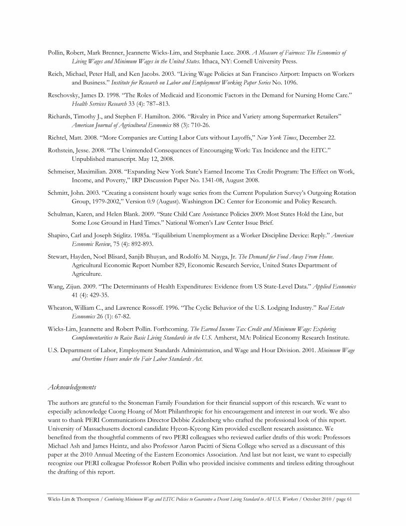
Wicks-Lim & Thompson / Combining Minimum Wage and EITC Policies to Guarantee a Decent Living Standard to All U.S. Workers / October 2010 / page 61
Pollin, Robert, Mark Brenner, Jeannette Wicks-Lim, and Stephanie Luce. 2008. A Measure of Fairness: The Economics of Living Wages and Minimum Wages in the United States. Ithaca, NY: Cornell University Press.
Reich, Michael, Peter Hall, and Ken Jacobs. 2003. “Living Wage Policies at San Francisco Airport: Impacts on Workers and Business.” Institute for Research on Labor and Employment Working Paper Series No. 1096.
Reschovsky, James D. 1998. “The Roles of Medicaid and Economic Factors in the Demand for Nursing Home Care.” Health Services Research 33 (4): 787–813.
Richards, Timothy J., and Stephen F. Hamilton. 2006. “Rivalry in Price and Variety among Supermarket Retailers” American Journal of Agricultural Economics 88 (3): 710-26.
Richtel, Matt. 2008. “More Companies are Cutting Labor Cuts without Layoffs,” New York Times, December 22.
Rothstein, Jesse. 2008. “The Unintended Consequences of Encouraging Work: Tax Incidence and the EITC.” Unpublished manuscript. May 12, 2008.
Schmeiser, Maximilian. 2008. “Expanding New York State’s Earned Income Tax Credit Program: The Effect on Work, Income, and Poverty,” IRP Discussion Paper No. 1341-08, August 2008.
Schmitt, John. 2003. “Creating a consistent hourly wage series from the Current Population Survey’s Outgoing Rotation Group, 1979-2002,” Version 0.9 (August). Washington DC: Center for Economic and Policy Research.
Schulman, Karen, and Helen Blank. 2009. “State Child Care Assistance Policies 2009: Most States Hold the Line, but Some Lose Ground in Hard Times.” National Women’s Law Center Issue Brief.
Shapiro, Carl and Joseph Stiglitz. 1985a. “Equilibrium Unemployment as a Worker Discipline Device: Reply.” American Economic Review, 75 (4): 892-893.
Stewart, Hayden, Noel Blisard, Sanjib Bhuyan, and Rodolfo M. Nayga, Jr. The Demand for Food Away From Home. Agricultural Economic Report Number 829, Economic Research Service, United States Department of Agriculture.
Wang, Zijun. 2009. “The Determinants of Health Expenditures: Evidence from US State-Level Data.” Applied Economics 41 (4): 429-35.
Wheaton, William C., and Lawrence Rossoff. 1996. “The Cyclic Behavior of the U.S. Lodging Industry.” Real Estate Economics 26 (1): 67-82.
Wicks-Lim, Jeannette and Robert Pollin. Forthcoming. The Earned Income Tax Credit and Minimum Wage: Exploring Complementarities to Raise Basic Living Standards in the U.S. Amherst, MA: Political Economy Research Institute.
U.S. Department of Labor, Employment Standards Administration, and Wage and Hour Division. 2001. Minimum Wage and Overtime Hours under the Fair Labor Standards Act.
Acknowledgements
The authors are grateful to the Stoneman Family Foundation for their financial support of this research. We want to especially acknowledge Cuong Hoang of Mott Philanthropic for his encouragement and interest in our work. We also want to thank PERI Communications Director Debbie Zeidenberg who crafted the professional look of this report. University of Massachusetts doctoral candidate Hyeon-Kyeong Kim provided excellent research assistance. We benefited from the thoughtful comments of two PERI colleagues who reviewed earlier drafts of this work: Professors Michael Ash and James Heintz, and also Professor Aaron Pacitti of Siena College who served as a discussant of this paper at the 2010 Annual Meeting of the Eastern Economics Association. And last but not least, we want to especially recognize our PERI colleague Professor Robert Pollin who provided incisive comments and tireless editing throughout the drafting of this report.