Embed Size (px)
Citation preview
DOCUMENTOS DE TRABAJO
Sovereign Bond Spreads and Extra-Financial Performance: An Empirical Analysis of Emerging Markets
Florian BergPaula MargareticSébastien Pouget
N.º 789 Agosto 2016BANCO CENTRAL DE CHILE
BANCO CENTRAL DE CHILE
CENTRAL BANK OF CHILE
La serie Documentos de Trabajo es una publicación del Banco Central de Chile que divulga los trabajos de investigación económica realizados por profesionales de esta institución o encargados por ella a terceros. El objetivo de la serie es aportar al debate temas relevantes y presentar nuevos enfoques en el análisis de los mismos. La difusión de los Documentos de Trabajo sólo intenta facilitar el intercambio de ideas y dar a conocer investigaciones, con carácter preliminar, para su discusión y comentarios.
La publicación de los Documentos de Trabajo no está sujeta a la aprobación previa de los miembros del Consejo del Banco Central de Chile. Tanto el contenido de los Documentos de Trabajo como también los análisis y conclusiones que de ellos se deriven, son de exclusiva responsabilidad de su o sus autores y no reflejan necesariamente la opinión del Banco Central de Chile o de sus Consejeros.
The Working Papers series of the Central Bank of Chile disseminates economic research conducted by Central Bank staff or third parties under the sponsorship of the Bank. The purpose of the series is to contribute to the discussion of relevant issues and develop new analytical or empirical approaches in their analyses. The only aim of the Working Papers is to disseminate preliminary research for its discussion and comments.
Publication of Working Papers is not subject to previous approval by the members of the Board of the Central Bank. The views and conclusions presented in the papers are exclusively those of the author(s) and do not necessarily reflect the position of the Central Bank of Chile or of the Board members.
Documentos de Trabajo del Banco Central de ChileWorking Papers of the Central Bank of Chile
Agustinas 1180, Santiago, ChileTeléfono: (56-2) 3882475; Fax: (56-2) 3882231

Documento de Trabajo
N° 789
Working Paper
N° 789
SOVEREIGN BOND SPREADS AND EXTRA-FINANCIAL
PERFORMANCE: AN EMPIRICAL ANALYSIS OF
EMERGING MARKETS
Florian Berg
Universidad Paris-Dauphine
Amundi Asset Management
Paula Margaretic
Banco Central de Chile
Sébastien Pouget
Toulose School of Economics
IDEI
Abstract
This paper studies the impact of a country's extra-financial performance on their sovereign bond
spreads. Sovereign bond spreads reflect both an economic default risk and a strategic default risk.
We hypothesize that a country's extra-financial performance reduces default risk by signaling good
commitment ability. We test this hypothesis for the countries which bonds are included in the JP
Morgan Emerging Markets Bond Index Global. Over the period from 2001 to 2010, we find that an
emerging country's average cost of capital decreases with its environmental and social performance.
Resumen
Este trabajo estudia el impacto de la información extra-financiera en los spreads de los bonos
soberanos. Los spreads soberanos reflejan dos tipos de riesgos de no pago: un riesgo de no pago
económico y otro estratégico. Nuestra hipótesis es que la información extra-financiera de un país
reduce el riesgo de no pago estratégico, en la medida que refleja un buen compromiso. Testeamos
esta hipótesis para los países, cuyos bonos soberanos forman parte del Indice Global de Bonos de
Mercados Emergentes del JPMorgan. Usando datos entre los años 2001-2010, encontramos que el
costo de capital promedio en estos países se reduce cuando la performance ambiental y/o social
mejora.
We thank Marie Brière, Patricia Crifo, and Rim Oueghlissi for helpful comments. We gratefully acknowledge support
from the Center on Sustainable Finance and Responsible Investment (“Chaire Finance Durable et Investissement
Responsable") at IDEI-R. Remaining errors are naturally ours. Emails: [email protected], [email protected] y
1 Introduction
This paper studies the link between a country’s sovereign bond returns and its extra-financial
performance, as measured by Environmental, Social and Governance (ESG) variables. Similar to
corporate bonds, government bonds bear a risk of economic default in case of major macroeconomic
downturns. But government bonds also bear a strategic default risk to the extent that governments
can repudiate their debt due to their sovereignty privilege.
A good extra-financial performance at the country level might serve three distinct economic
roles. First, a good performance might signal a country’s long-term orientation and may thus act
as a credible commitment to repay its debt in the future. Second, to the extent that exploiting
natural resources and social development requires the collaboration of outside parties (like foreign
countries or large foreign private organizations), countries with sound extra-financial performance
might have more to loose in case of default: They would not only loose some future opportunities
to borrow, but also loose part of the future benefits from its natural and social resources. Third, a
country’s natural and social resources might have a direct long term economic impact, acting as a
buffer against negative economic shocks or having a positive impact on future growth.
In this paper, we test whether emerging countries with good ESG performance, have a lower
(economic and/or strategic) risk of default and therefore, a lower cost of debt. We focus on emerging
countries for two reasons. First, the risk of default is pretty prevalent. This can be seen in the
significant number of emerging countries which have experienced default episodes since 2000 (e.g.,
Argentina, Ecuador, Dominican Republic, Gabon, Nigeria, Venezuela and Ukraine).
Second, ESG issues are particularly acute for emerging countries. For example, the Environ-
mental Performance Index (EPI), published annually by Yale University, appears pretty low in
2010 for the countries included in the Emerging Market Bond Index Global, ranging from 25 (for
Iraq) to 64 (for Croatia). This has to be compared to the average EPI score for OECD countries
which equals 72 for the same year.
To measure the cost of debt, we focus on government bond spreads as provided by the JP
Morgan’s EMBI Global database.1 The data sample is 2001 − 2010. To proxy a country’s extra-
financial performance, we use three indices on Environmental, Social and Governance issues: the
Environmental Performance Index (constructed by Yale University), the Human Development Index
and the World Governance Index (both from the World Bank), respectively.
The environmental performance reflects how well countries manage their natural resources (ac-
cess to water, biodiversity, etc), while the social performance measures the countries’ human devel-
opment (literacy rate, education enrollment ratios, life expectancy, among others). The governance
1The spread is the government bond interest rate minus the US government bond rate.
1
indicator, in turn, covers issues such as government effectiveness, regulatory quality, rule of law,
control of corruption, voice and accountability, political stability and no violence. Finally, we
also use additional data to build control variables related to technical bond issues, macroeconomic
conditions and sovereign credit ratings.
We use an estimation based on the Generalized Method of Moments (GMM) which enables to
regress the government bond spreads, as a function of the ESG indicators and the various control
variables. Because of the long-run features of the macroeconomic control variables and the ESG
factor correlation, we introduce various autoregressive variables in the estimation.
Overall, our results show that a good country’s ESG performance is associated with a lower cost
of debt. Furthermore, the evidence presented below suggests a dual effect of the ESG factors. On
the one hand, the governance indicator is negatively associated with contemporaneous government
bond spreads. On the other hand, the environmental and social factors are positively associated
with contemporaneous government bond spreads and negatively associated with future spreads.
These results are robust to alternative specifications of the variables used to proxy the country-
specific macroeconomic conditions.
This last result indicates that changes in a country’s environmental and social performance
take some time to be incorporated by financial markets. This seems intuitive since the impact
of environmental and social performance is likely to have a long-term impact that is difficult to
evaluate. Interestingly, our results are in line with Crifo et al. (2014)’s conclusion that the cost of
debt of 23 OECD countries is lower due to a sound ESG performance of the issuer.
Practical implications of our results are twofold. First, these results indicate that environmen-
tal, social and governance factors are priced by sovereign bond markets, good ESG performance
being associated with less default risk and thus lower cost of debt. Such a conclusion is interesting
for governments and policy makers, concerned about the determinants of the cost of sovereign debt.
It is also relevant for responsible asset managers and investors who screen investment opportuni-
ties based on ESG criteria to avoid investing in countries that are not acting in accordance with
international norms.2 These institutions rely on the same type of information as we do, given
the non-availability of high frequency data. Second, these results suggest that tactical portfolio
reallocations, based on observed changes in countries ESG performance, might improve sovereign
bond portfolios risk-adjusted returns.
The remainder of the paper is organized as follows. Section 2 reviews the related literature,
2An example of asset management firm who uses ESG factors to design its investment policy is Global Evolution,
as indicated in its sovereign screening process at globalevolution.com. The Norway sovereign pension fund global is
another example of a responsible investor who uses ethical principles to screen potential investments in foreign coun-
tries, as explained at regjeringen.no/en/topics/the-economy/the-government-pension-fund/responsible-investments.
2
whereas section 3 describes the Hypothesis we test in this paper. Section 4 presents the data
and the methodology. Section 5 displays the empirical results and discusses the main findings of
the paper. Finally, section 6 concludes. The appendix contains additional details and descriptive
statistics, absent in the main text.
2 Literature Review
Our paper is related to two strands of literature.
First, there is the abundant literature on the empirical determinants of emerging markets (EM)
sovereign bond spreads. Although the list of drivers this strand identifies is long, it is possible to
classify them into two groups. On one hand, global factors, also known as ”push” factors, such
as, capital flows, international interest rates and risk appetite, international terms of trades and
external shocks. On the other hand, country-specific macroeconomic variables or ”pull” factors,
like GDP growth, international reserves, export growth, fiscal and current account balance, public
investment, inflation and sovereign credit ratings. Among the most recent contributions, it is pos-
sible to cite Gonzalez-Rozada and Levy Yeyati (2008), Hilscher and Nosbusch (2010) and Kennedy
and Palerm (2014).
One focus of this literature has been to determine whether the pull or push factors dominate.
As some illustrations, Gonzalez-Rozada and Levy Yeyati (2008) find that over 1993− 2005, a large
fraction of the time variability of EMBI spreads has been explained by the evolution of global
factors, such as risk appetite, global liquidity and contagion from systemic events. Kennedy and
Palerm (2014), in turn, find that much of the decline in the EMBI spreads from 2002 to 2007 reflects
improved country-specific fundamentals, but their sharp increase in the 2008 crisis has been due to
risk aversion.3
Second, there is the strand examining the impact of environmental, social and governance
factors on sovereign bond spreads or sovereign credit ratings. The majority of articles consider the
governance indicators as a way to proxy these soft factors.4 Among them, Ciocchini et al. (2003)
and Depken et al. (2011) focus on corruption; Moser (2007), Baldacci et al. (2011) and Bekaert et
al. (2014) concentrate on political risk and finally, Cosset and Jeanneret (2014) and Benzoni et al.
(2015) examine the impact of government effectiveness and political stability, respectively.5
3Instead of EMBI spreads, several authors have looked at sovereign Credit Default Swap data. Some examples
are Remolona et al. (2008), Longstaff et al. (2010) and Amstad et al. (2016).4Most of them also include global and macro-economic country-specific variables, as additional covariates.5Ciocchini et al. (2003) and Depken et al. (2011) rely on the Transparency International Corruption Perception
Index; Baldacci et al. (2011) use the International Country Risk Guide Political Risk Indicator and Bekaert et al.
(2014) elaborate their own index, based on the World Bank Governance Indicators. Finally, Cosset and Jeanneret
3
Overall, these studies conclude that governance indicators matter to explain credit risk in
emerging markets. For instance, Ciocchini et al. (2003) show that emerging countries that are
perceived as more corrupt must pay a higher risk premium when issuing bonds, while Baldacci et
al. (2011) find that lower levels of political risk are associated with tighter sovereign bond spreads,
particularly during financial turmoil.
Only two studies investigate how a broad measure of environmental, social and governance
factors affect sovereign bond markets. First, Drut (2010) investigates how the mean efficient frontier
of portfolios containing sovereign bonds from 20 developed countries changes, due to an integration
of ESG factors. He concludes that an integration of ESG factors in sovereign bond portfolios does
not affect the efficient frontier and thus the financial performance.
Second, Crifo et al. (2014) show that the cost of debt of 23 OECD countries, as measured by
sovereign bond yield spreads, is lower due to a sound ESG performance of the issuer. The ESG
performance is measured by Vigeo ratings. In addition, they show that the positive effect of ESG
ratings on the cost of debt decreases with bond maturities.
We contribute to the aforementioned strands of literature, since in addition to global and
country-specific macroeconomic variables, we examine whether ESG factors are significant non-
economic, long-run determinants of EM sovereign bond spreads. To our best knowledge, we are
first to examine these factors for emerging markets.
3 Hypothesis
The reasons why countries ever pay back their debt have been the object of a long standing debate
in economics. Their sovereignty indeed does not put them under external authority to impose
repayment. One reason for repayment as highlighted for example by Eaton and Gersovitz (1981)
is that sovereign entities want to maintain a good reputation to ensure future access to borrowing.
In this case, the more long-term oriented a country is, the more important its reputation is, and
the less likely its default.
This logic has been questioned by Bulow and Rogoff (1989) on the ground that credibility for
repayment is very hard to establish: After a country has borrowed, it has an incentive to use any
money obtained or generated by positive fiscal shocks to invest and smooth future negative shocks
with these savings, thus not depending on future borrowing capacities. Bulow and Rogoff (1989)
then show that additional sanctions, above the fact of not lending, should be exercised in order for
sovereign entities to be able to borrow.
(2014) rely on the World Bank Governance Indicators.
4

Cole and Kehoe (1994) elaborate on this idea by indicating that the threat of terminating non-
lending relationships such as collaborations to exploit common resources, as suggested by Conklin
(1998), might induce countries to repay in order to preserve these agreements. Dhillon et al.
(2013) further show that borrowing countries and their lenders might be involved in long-term
relationships, aside from the lending ones, that may also enable lenders to impose penalties on
borrowers in case of default. This reduces the risk of default on the sovereign borrower. Overall, in
these models, sovereign countries repay their debt because they are concerned about their long-term
reputation. Finally, following the insight of Grossman and Van Huyk (1988), sovereign (partial)
default might be viewed as an efficient way of smoothing shocks over time (countries pay back when
they are rich but pay back less when they are poor).
Given these conceptual considerations, a good extra-financial performance at the country level
might serve three distinct economic roles. First, to the extent that extra-financial performance
mostly materializes in economic benefits in the long term, a good performance might act as a
signal of a country’s long-term orientation. Second, to the extent that exploiting natural resources
and social development requires the collaboration of outside parties (like foreign countries or large
foreign private organizations), countries with a high level of extra-financial performance might have
more to loose in case of default, because they would not only loose future opportunities to borrow
but also loose part of the future benefits from its natural and social resources. Third, a country’s
natural and social resources might act as a buffer against negative shocks. Finally, another reason
why a good extra-financial performance might be associated with a lower cost of debt is that ESG
factors might have a positive impact on future growth and thus on the future ability to repay.
These considerations indicate that countries with a good extra-financial performance should have
a lower (economic and/or strategic) risk of default and thus a lower cost of debt. This leads to the
following Hypothesis.
Hypothesis 1: There is a negative link between a good environmental, social and governance
performance and the cost of debt, as measured by sovereign spreads.
We focus here on the cost of debt, as measured by the spread over the US interest rate, because
it is more easily observable then actual defaults which occur pretty infrequently. Moreover, it
is obviously likely that other factors than the extra-financial performance of a country affect its
spread. We thus include a number of control variables in our analysis, including sovereign credit
ratings and macroeconomic variables.
5
4 Data and Methodology
4.1 Data
4.1.1 Bond Data
We use bond data on the JP Morgan’s EMBI Global, from 2001 to 2010. The EMBI Global
tracks total returns of dollar-denominated sovereign bonds, issued by emerging market countries.
We consider the country-specific subindexes of 33 emerging economies. Debt instruments in (each
country-specific subindex of) the EMBI Global must have a minimum face value outstanding of
500 million dollars. We choose the stripped mid-point spread, as our measure for the cost of debt.
It corresponds to the zero-volatility spread over the US zero-coupon yield curve.
Furthermore, JP Morgans strips away those cash flows that are guaranteed by the US govern-
ment, e.g. Brady bonds. We then take the arithmetic average of the monthly spreads for each
year (which we name hereafter as Spread). In addition, we use the Bid Ask spread (hereafter, Bid
Ask), to measure liquidity; the average life (Average Life) of the country-specific subindex and
the squared average life (Average Life Squared), to measure duration and convexity, respectively.
Finally, we rely on Fitch’s long term credit rating (hereafter, Rating) to measure credit worthiness.6
4.1.2 Macroeconomic Control Variables
GDP Growth (GDP Growth) is a risk score from 0 to 10 that includes current and expected growth.
It is part of the International Country Risk Guide (ICRG) from the Political Risk Services (PRS)
group. We use the general government gross debt (which we denote hereafter as Gov Debt), to
measure the government’s performance in managing its public finances.
4.1.3 Environmental, Social and Governance Data
The environmental indicator is based on the Environmental Performance Index (EPI ) con-
structed by Yale University. EPI covers environmental health, corresponding to the protection of
human health (for instance, access to water and sanitation) and ecosystem vitality, corresponding
6Fitch makes both a qualitative and quantitative assessment of the sovereign creditworthiness to construct their
sovereign ratings. The quantitative evaluation is mainly based on economic and financial variables, corresponding to
structural features (such as GDP per capita and aggregate money supply), macroeconomic performance (like GDP
growth), public finances (e.g. the stock of debt and fiscal balance) and external balance (as the current account).
To complement the quantitative assessment, Fitch adds an evaluation of each sovereign’s country risk. The latter
includes a variety of dimensions, ranging from the level of corruption, the functionality of the administration to the
perception of potential social unrest.
6

to the impact of human activities on the natural environment (e.g., biodiversity). EPI scores range
from 0 (worst) to 100 (best).
The human development index (hereafter HDI ) combines three measures that proxy for
human development. First, it contains knowledge and education, as measured by the adult literacy
rate and the combined primary, secondary, and tertiary gross enrollment ratio. Second, it includes
the standard of living, as indicated by the natural logarithm of GDP per capita at purchasing
power parity. Third, it integrates life expectancy at birth. The data source is World Bank.
The governance indicator is based on the World Governance Indicators constructed by the
World Bank. These indicators cover issues such as government effectiveness, regulatory quality,
rule of law, control of corruption, voice and accountability, political stability and non violence.
Each indicator is normally distributed, with mean 0, standard deviation of 1 and ranges from
approximately −5 to 5, with higher values corresponding to better governance.
Following common practice, we add them up, to create the variable WGIT.7 Appendix A
contains a detailed description of each indicator, together with the correlation matrix between
them. Table 1 shows the descriptive statistics, while figures 1 and 2 depict the box plot of Spread
and the ESG factors, namely, EPI, HDI and WGIT, at each point in time.
7See for example, Butler and Fauver (2006).
7
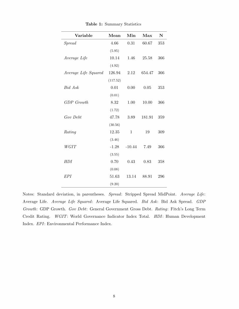
Table 1: Summary Statistics
Variable Mean Min Max N
Spread 4.66 0.31 60.67 353
(5.95)
Average Life 10.14 1.46 25.58 366
(4.92)
Average Life Squared 126.94 2.12 654.47 366
(117.52)
Bid Ask 0.01 0.00 0.05 353
(0.01)
GDP Growth 8.32 1.00 10.00 366
(1.72)
Gov Debt 47.78 3.89 181.91 359
(30.56)
Rating 12.35 1 19 309
(3.46)
WGIT -1.28 -10.44 7.49 366
(3.55)
HDI 0.70 0.43 0.83 358
(0.08)
EPI 51.63 13.14 88.91 296
(9.20)
Notes: Standard deviation, in parentheses. Spread : Stripped Spread MidPoint. Average Life:
Average Life. Average Life Squared : Average Life Squared. Bid Ask : Bid Ask Spread. GDP
Growth: GDP Growth. Gov Debt : General Government Gross Debt. Rating : Fitch’s Long Term
Credit Rating. WGIT : World Governance Indicator Index Total. HDI : Human Development
Index. EPI : Environmental Performance Index.
8

Figure 1: Box plot of Spread (left) and WGIT (right), by year
Notes: Red points depict annual median values. Spread : Stripped Spread MidPoint. WGIT :
World Governance Indicator Index Total.
Figure 2: Box plot of HDI (left) and EPI (right), by year
Notes: Red points depict annual median values. HDI : Human Development Index. EPI : Environ-
mental Performance Index.
Two comments are at place. First, tables 1 and figures 1 and 2 outline the evolution of Spread, as
well as the heterogeneity between countries, in terms of their environmental, social and governance
performance. For instance, if we consider the environmental dimension, not all the considered
economies take care of their natural resources in the same way. Indeed, in 2010, the EPI score
ranges from 25 (for Iraq) to 64 (for Croatia). To put the latter figures into perspective, the average
EPI score for OECD countries equals 72 for the same year.
Second, over the period, some emerging economies have experienced significant disruptive
episodes. For example, Argentina, Venezuela, Dominican Republic, Ecuador, Nigeria and Gabon
9

have suffered sovereign debt crisis,8 whereas Lebanon entered in war in 2006.9 Critical events
like the aforementioned ones may not be well captured by the commonly used empirical determi-
nants of Spread (see section 2). The inclusion of the ESG factors aims at capturing the impact of
extra-financial performance information on emerging markets’ cost of debt.
In order to assess the informational content of the ESG factors relative to the country-specific
macroeconomic variables, we conduct the following exercise. We first construct quartiles, based
on the empirical distribution of each ESG factor and Rating, the latter summarizing the country-
specific macroeconomic determinants. We then look at whether countries with good (bad) ESG
performance tend to coincide with those with high (low) credit scores.
Tables 2, 3 and 4 present bivariate contingency tables between the quartiles of each ESG factor
and Rating, as well as the mean and standard deviation of Rating, for each quartile of the ESG
factors. Recall that higher values of the four variables correspond to better performance.
Interestingly, tables 2, 3 and 4 suggest a distinct pattern between the environmental and so-
cial factors, on one hand, and the governance indicator, on the other: While countries with good
environmental and social indicators may not necessarily be those with sound macroeconomic per-
formance, as measured by credit scores, the evidence on WGIT depicts a positive relationship with
Rating.
As an illustration, if we look at the diagonal elements of the bivariate contingency tables (left
blocks of tables 2, 3 and 4), the number of matches between WGIT and Rating, by quartile, is much
higher than in the other two bivariate comparisons. The latter is reflecting that Fitch Credit Rating
Agency takes this information into account when evaluating the financial health of a country, as
described in its credit rating model documentation.
8We define sovereign debt crisis as episodes at which the sovereign was unable to meet its obligations, as they
became due. The latter definition thus includes sovereign defaults and/or sovereign debt restructuring plans.9As an illustration, the WGIT score of Lebanon in 2006 is −4.34, below the −2.93 average WGIT score of the
countries in our dataset belonging to the same region.
10

Table 2: Bivariate contingency table between the quartiles of EPI and Rating (left block) and
mean and standard deviation of Rating, for each quartile of EPI (last column)
Rating
Quartiles of 1 2 3 4 Rating
EPI
1 7.14 24.64 17.65 31.8813.71
(0.39)
2 41.43 34.78 23.53 7.2510.97
(0.30)
3 32.86 20.29 22.06 30.4311.91
(0.53)
4 18.57 20.29 36.76 30.4312.92
(0.38)
Total 100.00 100.00 100.00 100.00
Notes: Standard deviation, in parentheses. Rating: Fitch’s Long Term Credit Rating. EPI: Environmental
Performance Index.
Table 3: Bivariate contingency table between the quartiles of HDI and Rating (left block) and
mean and standard deviation of Rating, for each quartile of HDI (last column)
Rating
Quartiles of 1 2 3 4 Rating
HDI
1 7.46 27.27 28.57 18.4213.21
(0.30)
2 44.78 42.42 17.46 6.5810.94
(0.35)
3 32.84 18.18 41.27 21.0512.23
(0.36)
4 14.93 12.12 12.7 53.9513.65
(0.59)
Total 100.00 100.00 100.00 100.00
Notes: Standard deviation, in parentheses. Rating: Fitch’s Long Term Credit Rating. HDI: Human Development
Index.
11

Table 4: Bivariate contingency table between the quartiles of WGIT and Rating (left block) and
mean and standard deviation of Rating, for each quartile of WGIT (last column)
Rating
Quartiles of 1 2 3 4 Rating
WGIT
1 37.97 26.32 5.19 10.3910.47
(0.36)
2 29.11 40.79 24.68 12.9911.63
(0.40)
3 26.58 23.68 45.45 7.7911.68
(0.34)
4 6.33 9.21 24.68 68.8315.09
(0.26)
Total 100.00 100.00 100.00 100.00
Notes: Standard deviation, in parentheses. Rating: Fitch’s Long Term Credit Rating. WGIT: World Governance
Indicator Index Total.
In the next section, we present the methodology we use to test the Hypothesis 1.
4.2 Methodology
The estimation technique is a dynamic panel data regression. This is because the data show that
Spread are persistent. More specifically, we follow a GMM estimation, through which we regress
the difference of Spread, as a function of the first lagged difference of Spread, the previously defined
subindex-specific and macroeconomic control variables and the ESG factors, all in first differences.10
For the estimation, we use the Arellano-Bover (1995)/Blundell-Bond (1998) estimator, also known
as system GMM;11 in particular, we consider the one−step System GMM. Finally, the to-be re-
ported standard errors are robust to the presence of both arbitrary heteroskedasticity and serial
correlation.
10Using dummy variables to estimate individual (country-specific) fixed-effects in a model which also includes a
lagged value of the dependent variable results in biased estimates, when the time dimension T of the panel is small
(in our case, T = 10). This problem is widely known in the literature as the Dynamic Panel Bias or Nickel Bias.
That is why we first need to difference the equation to estimate and then instrument the first lagged difference of
Spread.11As Blundell and Bond (1998) and Blundell et al. (2000) point out, system GMM is particularly adequate (over
Difference GMM) for applications with persistent series. To implement it, we use the xtabond2 command, available
in Stata 14.1.
12
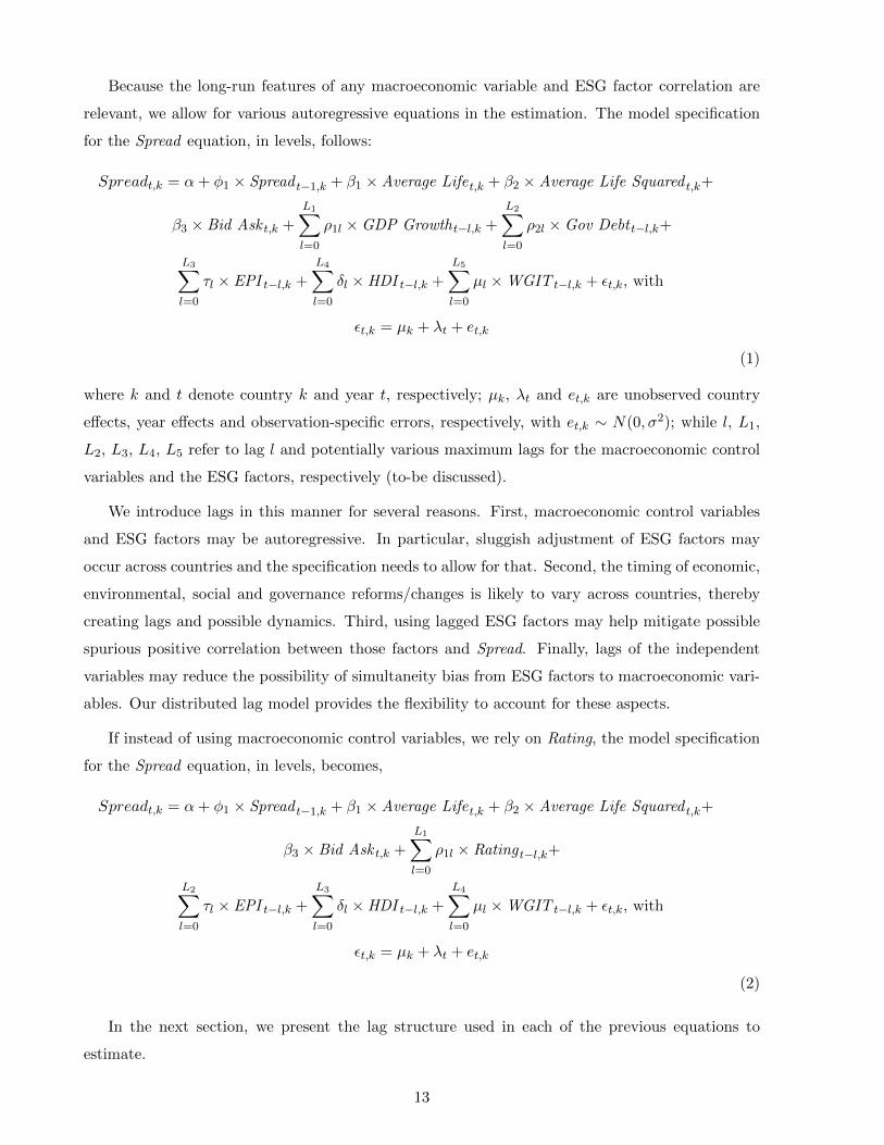
Because the long-run features of any macroeconomic variable and ESG factor correlation are
relevant, we allow for various autoregressive equations in the estimation. The model specification
for the Spread equation, in levels, follows:
Spreadt,k = α+ φ1 × Spread t−1,k + β1 ×Average Lifet,k + β2 ×Average Life Squared t,k+
β3 × Bid Ask t,k +
L1∑l=0
ρ1l ×GDP Growtht−l,k +
L2∑l=0
ρ2l ×Gov Debt t−l,k+
L3∑l=0
τl × EPI t−l,k +
L4∑l=0
δl ×HDI t−l,k +
L5∑l=0
µl ×WGIT t−l,k + εt,k, with
εt,k = µk + λt + et,k
(1)
where k and t denote country k and year t, respectively; µk, λt and et,k are unobserved country
effects, year effects and observation-specific errors, respectively, with et,k ∼ N(0, σ2); while l, L1,
L2, L3, L4, L5 refer to lag l and potentially various maximum lags for the macroeconomic control
variables and the ESG factors, respectively (to-be discussed).
We introduce lags in this manner for several reasons. First, macroeconomic control variables
and ESG factors may be autoregressive. In particular, sluggish adjustment of ESG factors may
occur across countries and the specification needs to allow for that. Second, the timing of economic,
environmental, social and governance reforms/changes is likely to vary across countries, thereby
creating lags and possible dynamics. Third, using lagged ESG factors may help mitigate possible
spurious positive correlation between those factors and Spread. Finally, lags of the independent
variables may reduce the possibility of simultaneity bias from ESG factors to macroeconomic vari-
ables. Our distributed lag model provides the flexibility to account for these aspects.
If instead of using macroeconomic control variables, we rely on Rating, the model specification
for the Spread equation, in levels, becomes,
Spreadt,k = α+ φ1 × Spread t−1,k + β1 ×Average Lifet,k + β2 ×Average Life Squared t,k+
β3 × Bid Ask t,k +
L1∑l=0
ρ1l × Rating t−l,k+
L2∑l=0
τl × EPI t−l,k +
L3∑l=0
δl ×HDI t−l,k +
L4∑l=0
µl ×WGIT t−l,k + εt,k, with
εt,k = µk + λt + et,k
(2)
In the next section, we present the lag structure used in each of the previous equations to
estimate.
13
5 Empirical Results
Tables 5 and 6 report the estimation of equations (1) and (2), respectively; the first one uses
macroeconomic variables as control, the second one uses Rating. In each table, there are several
columns of results, due to alternative lag structures for the macroeconomic control variables (or
the variable Rating) and the ESG factors and due to different combinations of control variables.
Starting with table 5, in its first column of results, we include as covariates the first differenced
subindex-specific regressors, which are standardized, as well as the macroeconomic control variables.
The second column adds to the first one the differenced ESG factors, also standardized, which enter
contemporaneously in the equation to estimate. The third column of results, in turn, allows for
distinct lag structures for the macroeconomic control variables, on one hand, and the ESG factors,
on the other hand.
More specifically, while the differenced macroeconomic control variables enter contemporane-
ously and with their first lag, in the case of the ESG factors, we include their first as well as their
second lag. Finally, in the fourth column of results, we augment the third model specification with
a dummy variable that takes the value of 1 if the country has experienced a sovereign debt crisis
over the sample period.
The motivation behind the distinct lag structure for the macroeconomic control variables, on
one hand, and the ESG factors, on the other hand, is as follows. Regarding the first group, the
inclusion of their first lag (in the third and fourth column of results of table 5) is for robustness.
Concerning the ESG factors, they seem to be autoregressive, in particular, the environmental and
social factors. The correlation matrix of the differenced ESG factors and their lags in Appendix A
provides evidence in favor of the environmental and social factors being moving slowly.
Table 6, in turn, reports the model estimates of equation (2), this time with Rating summa-
rizing the macroeconomic control variables. As before, there are several columns of results, due to
alternative lag structures and different combinations of covariates. The only difference with table
5 is that table 6 no longer reports the model estimates without the ESG factors.
14
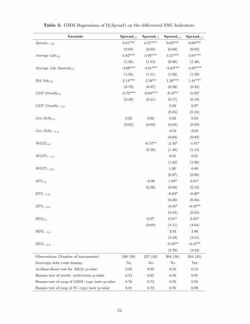
Table 5: GMM Regressions of D(Spread) on the differenced ESG Indicators.
Variable Spreadt,k Spreadt,k Spreadt,k Spreadt,k
Spread t−1,k 0.61*** 0.57*** 0.63*** 0.60***
(0.02) (0.03) (0.03) (0.02)
Average Lifet,k 3.82*** 3.93*** 3.21*** 3.91***
(1.36) (1.53) (0.98) (1.38)
Average Life Squared t,k -3.60*** -3.81*** -3.24*** -4.07***
(1.28) (1.51) (1.02) (1.50)
Bid Ask t,k 2.14*** 2.28** 1.50*** 1.41***
(0.79) (0.87) (0.39) (0.35)
GDP Growtht,k -0.72*** -0.63*** -0.37** -0.33*
(0.28) (0.21) (0.17) (0.18)
GDP Growtht−1,k 0.02 0.07
(0.25) (0.23)
Gov Debtt,k 0.02 0.02 0.02 0.03
(0.02) (0.02) (0.03) (0.03)
Gov Debtt−1,k -0.01 -0.01
(0.03) (0.03)
WGIT t,k -0.74** -2.44* -1.81*
(0.36) (1.46) (1.13)
WGIT t−1,k 0.85 0.91
(1.82) (1.66)
WGIT t−2,k 1.26� 0.89
(0.87) (0.96)
EPI t,k -0.06 1.09* 0.91*
(0.30) (0.60) (0.53)
EPI t−1,k -0.63* -0.66*
(0.36) (0.36)
EPI t−2,k -0.44* -0.45**
(0.24) (0.24)
HDIt,k 0.97� 6.81* 6.63*
(0.69) (4.11) (4.04)
HDIt−1,k 2.03 2.06
(3.59) (3.51)
HDIt−2,k -8.34** -8.27**
(3.76) (3.44)
Observations (Number of instruments) 240 (39) 237 (42) 204 (38) 204 (45)
Sovereign debt crisis dummy No No No Yes
Arellano-Bond test for AR(2) p-value 0.85 0.95 0.18 0.15
Hansen test of overid. restrictions p-value 0.54 0.61 0.39 0.97
Hansen test of exog of GMM−type instr p-value 0.76 0.72 0.76 0.93
Hansen test of exog of IV−type instr p-value 0.81 0.72 0.76 0.99
15
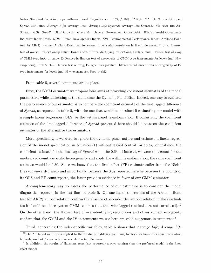
Notes: Standard deviation, in parentheses. Level of significance : � 15% ,* 10% , ** 5 % , *** 1%. Spread : Stripped
Spread MidPoint. Average Life: Average Life. Average Life Squared : Average Life Squared. Bid Ask : Bid Ask
Spread. GDP Growth: GDP Growth. Gov Debt : General Government Gross Debt. WGIT : World Governance
Indicator Index Total. HDI : Human Development Index. EPI : Environmental Performance Index. Arellano-Bond
test for AR(2) p-value: Arellano-Bond test for second order serial correlation in first differences, Pr > z. Hansen
test of overid. restrictions p-value: Hansen test of over-identifying restrictions, Prob > chi2. Hansen test of exog
of GMM-type instr p- value: Difference-in-Hansen test of exogeneity of GMM type instruments for levels (null H =
exogenous), Prob > chi2. Hansen test of exog, IV-type instr p-value: Difference-in-Hansen tests of exogeneity of IV
type instruments for levels (null H = exogenous), Prob > chi2.
From table 5, several comments are at place.
First, the GMM estimator we propose here aims at providing consistent estimates of the model
parameters, while addressing at the same time the Dynamic Panel Bias. Indeed, one way to evaluate
the performance of our estimator is to compare the coefficient estimate of the first lagged difference
of Spread, as reported in table 5, with the one that would be obtained if estimating our model with
a simple linear regression (OLS) or the within panel transformation. If consistent, the coefficient
estimate of the first lagged difference of Spread presented here should lie between the coefficient
estimates of the alternative two estimators.
More specifically, if we were to ignore the dynamic panel nature and estimate a linear regres-
sion of the model specification in equation (1) without lagged control variables, for instance, the
coefficient estimate for the first lag of Spread would be 0.63. If instead, we were to account for the
unobserved country-specific heterogeneity and apply the within transformation, the same coefficient
estimate would be 0.30. Since we know that the fixed-effect (FE) estimate suffer from the Nickel
Bias -downward-biased- and importantly, because the 0.57 reported here lie between the bounds of
its OLS and FE counterparts, the latter provides evidence in favor of our GMM estimator.
A complementary way to assess the performance of our estimator is to consider the model
diagnostics reported in the last lines of table 5. On one hand, the results of the Arellano-Bond
test for AR(2) autocorrelation confirm the absence of second-order autocorrelation in the residuals
(as it should be, since system GMM assumes that the twice-lagged residuals are not correlated).12
On the other hand, the Hansen test of over-identifying restrictions and of instrument exogeneity
confirm that the GMM and the IV instruments we use here are valid exogenous instruments.13
Third, concerning the index-specific variables, table 5 shows that Average Life, Average Life
12The Arellano-Bond test is applied to the residuals in differences. Thus, to check for first-order serial correlation
in levels, we look for second-order correlation in differences.13In addition, the results of Hausman tests (not reported) always confirm that the preferred model is the fixed
effect model.
16
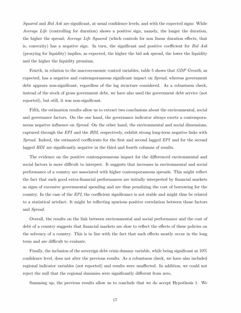
Squared and Bid Ask are significant, at usual confidence levels, and with the expected signs: While
Average Life (controlling for duration) shows a positive sign, namely, the longer the duration,
the higher the spread; Average Life Squared (which controls for non linear duration effects, that
is, convexity) has a negative sign. In turn, the significant and positive coefficient for Bid Ask
(proxying for liquidity) implies, as expected, the higher the bid ask spread, the lower the liquidity
and the higher the liquidity premium.
Fourth, in relation to the macroeconomic control variables, table 5 shows that GDP Growth, as
expected, has a negative and contemporaneous significant impact on Spread, whereas government
debt appears non-significant, regardless of the lag structure considered. As a robustness check,
instead of the stock of gross government debt, we have also used the government debt service (not
reported), but still, it was non-significant.
Fifth, the estimation results allow us to extract two conclusions about the environmental, social
and governance factors. On the one hand, the governance indicator always exerts a contempora-
neous negative influence on Spread. On the other hand, the environmental and social dimensions,
captured through the EPI and the HDI, respectively, exhibit strong long-term negative links with
Spread. Indeed, the estimated coefficients for the first and second lagged EPI and for the second
lagged HDI are significantly negative in the third and fourth columns of results.
The evidence on the positive contemporaneous impact for the differenced environmental and
social factors is more difficult to interpret. It suggests that increases in environmental and social
performance of a country are associated with higher contemporaneous spreads. This might reflect
the fact that such good extra-financial performances are initially interpreted by financial markets
as signs of excessive governmental spending and are thus penalizing the cost of borrowing for the
country. In the case of the EPI, the coefficient significance is not stable and might thus be related
to a statistical artefact: It might be reflecting spurious positive correlation between those factors
and Spread.
Overall, the results on the link between environmental and social performance and the cost of
debt of a country suggests that financial markets are slow to reflect the effects of these policies on
the solvency of a country. This is in line with the fact that such effects mostly occur in the long
term and are difficult to evaluate.
Finally, the inclusion of the sovereign debt crisis dummy variable, while being significant at 10%
confidence level, does not alter the previous results. As a robustness check, we have also included
regional indicator variables (not reported) and results were unaffected. In addition, we could not
reject the null that the regional dummies were significantly different from zero.
Summing up, the previous results allow us to conclude that we do accept Hypothesis 1. We
17
view the environmental, social and governance factors as non-economic determinants of the long
run evolution of Spread. Interestingly, our results are in line with Crifo et al. (2014), who, using a
sample of 23 OECD countries, find that the cost of debt is lower due to a sound ESG performance
of the issuer. Furthermore, they are indicative of a dual effect of the ESG factors: While the
governance indicator seems to have a contemporaneous impact on Spread, the environmental and
social factors exhibit a long-term negative influence on Spread.14
Table 6 reports the model estimates of equations (2), this time with Rating summarizing the
macroeconomic control variables.
14As a robustness check, we have extracted the Hodrick-Prescott (HP) trend of Spread. Using the latter as the
dependent variable, we have run a fixed effect estimator of the HP trend of Spread, as a function of the same
macroeconomic control variables, as well as the ESG factors. Interestingly, we find that the environmental and social
indicators continue to be significant and with the expected signs. Thus, it reinforces the conclusion that they are
significant non-economic long-term determinants of the long run Spread evolution.
18
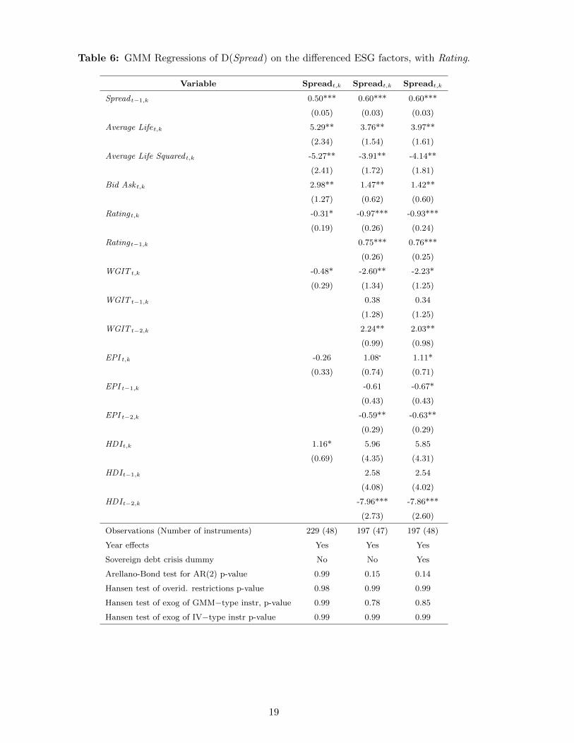
Table 6: GMM Regressions of D(Spread) on the differenced ESG factors, with Rating.
Variable Spreadt,k Spreadt,k Spreadt,k
Spread t−1,k 0.50*** 0.60*** 0.60***
(0.05) (0.03) (0.03)
Average Lifet,k 5.29** 3.76** 3.97**
(2.34) (1.54) (1.61)
Average Life Squared t,k -5.27** -3.91** -4.14**
(2.41) (1.72) (1.81)
Bid Ask t,k 2.98** 1.47** 1.42**
(1.27) (0.62) (0.60)
Ratingt,k -0.31* -0.97*** -0.93***
(0.19) (0.26) (0.24)
Ratingt−1,k 0.75*** 0.76***
(0.26) (0.25)
WGIT t,k -0.48* -2.60** -2.23*
(0.29) (1.34) (1.25)
WGIT t−1,k 0.38 0.34
(1.28) (1.25)
WGIT t−2,k 2.24** 2.03**
(0.99) (0.98)
EPI t,k -0.26 1.08� 1.11*
(0.33) (0.74) (0.71)
EPI t−1,k -0.61 -0.67*
(0.43) (0.43)
EPI t−2,k -0.59** -0.63**
(0.29) (0.29)
HDIt,k 1.16* 5.96 5.85
(0.69) (4.35) (4.31)
HDIt−1,k 2.58 2.54
(4.08) (4.02)
HDIt−2,k -7.96*** -7.86***
(2.73) (2.60)
Observations (Number of instruments) 229 (48) 197 (47) 197 (48)
Year effects Yes Yes Yes
Sovereign debt crisis dummy No No Yes
Arellano-Bond test for AR(2) p-value 0.99 0.15 0.14
Hansen test of overid. restrictions p-value 0.98 0.99 0.99
Hansen test of exog of GMM−type instr, p-value 0.99 0.78 0.85
Hansen test of exog of IV−type instr p-value 0.99 0.99 0.99
19
Notes: Standard deviation, in parentheses. Level of significance : � 15%, * 10% , ** 5 % , *** 1%. Spread : Stripped
Spread MidPoint. Average Life: Average Life. Average Life Squared : Average Life Squared. Bid Ask : Bid Ask
Spread. Rating : Fitch’s Long Term Credit Rating. WGIT : World Governance Indicator Index Total. HDI : Human
Development Index. EPI : Environmental Performance Index. Arellano-Bond test for AR(2) p-value: Arellano-Bond
test for second order serial correlation in first differences, Pr > z. Hansen test of overid. restrictions p-value: Hansen
test of over-identifying restrictions, Prob > chi2. Hansen test of exog of GMM-type instr p- value: Difference-in-
Hansen test of exogeneity of GMM type instruments for levels (null H = exogenous), Prob > chi2. Hansen test of
exog of IV-type instr p-value: Difference-in-Hansen tests of exogeneity of IV type instruments for levels (null H =
exogenous), Prob > chi2.
From table 6, several changes are worth to highlight, relative to table 5. First, interestingly,
Rating exhibits a significant negative contemporaneous impact on Spread, that is, the better the
country’s Rating, the lower the sovereign bond Spread. Moreover, this effect seems to persist, since
the first lag of the differenced Rating is also significant.
Second, in relation to the control variables, table 6 shows that overall, their coefficient estimates
only change in a minimal way, relative to table 5. Third, concerning the ESG factors, the similarity
of their estimated coefficients, relative to the previous table of results, seems encouraging: The
governance indicator continues to exert a contemporaneous negative influence on Spread, whereas
the environmental and social factors exhibit a strong negative long-term link with Spread.
However, in contrast to table 5, the second lagged coefficient estimates for the differenced gov-
ernance indicator (second and third column of results) are now positive and statistically significant,
regardless of whether we include the sovereign debt crisis dummy or not. We believe that the latter
may be due to a positive correlation between WGIT and Rating. Fitch’s credit rating model docu-
mentation, together with the evidence presented in section 4 that countries with good governance
indicators tend to coincide with those with sound macroeconomic performance, as measured by
Rating, reinforce this idea.
Summing up, thanks to the results reported in table 6, we continue to accept the Hypothesis
1, for the environmental, social and governance dimensions.
6 Conclusion
This paper studies the link between environmental, social, and governance (ESG) performance of a
country and its cost of debt. The idea is that such extra-financial performance can decrease default
risk either through a positive impact on future growth or through a positive signal regarding the
long term orientation of a country. We focus on emerging markets because the risk of default is
20
more prevalent and the ESG issues are more acute than in more developed countries.
We measure a country’s ESG performance by using well-established indicators: the Environ-
mental Performance Index constructed by Yale University for the environmental performance, the
Human Development Index constructed by the World Bank for the social performance, and the
World Governance Index constructed again by the World Bank for the governance performance of
a country. The cost of debt is measure by the spread between the rate of return offered by a coun-
try’s sovereign bond minus the one offered by the U.S. We include the bonds that are part of the
EMBI Global Index. We perform our regression analyses by using GMM. We include various con-
trol variables to account for macroeconomic conditions and technical issues related to fixed-income
instruments.
The first result from this study is that the ESG performance impacts the Spread. We view these
factors as non-economic determinants of the long run evolution of the Spread variable. Importantly,
they can have an impact on both types of default risk. On the one hand, sound ESG policies
might bring a strong and sustainable economic performance to a country, thereby reducing the
risk of economic default. On the other hand, a clear engagement towards sustainable development
might signal a country’s willingness to address long-term issues, and may thus act as a credible
commitment to repay its debt in the future. This might reduce the risk of strategic default.
Second, the environmental, social and governance factors exhibit a strong negative link with
Spread. Interestingly, our results are indicative of a dual effect of the ESG factors: While the
governance indicator seems to have a more contemporaneous impact on Spread, the environmental
and social factors exhibit a long-term negative influence on Spread. The environmental and so-
cial performance also has a positive link with the contemporaneous spreads, which suggests that
financial markets initially overemphasize the cost of the underlying public policies.
One possible explanation of the distinct behavior of the environmental and social factors, on
one hand, and the governance indicator, on the other hand, could be that the WGIT, as a measure
of country risk, has become a widely used piece of information. Furthermore, several studies have
shown their impact on Spread.
The impact of environmental and social indicators on Spread was less straightforward: An
increase in health expenditure or stricter air pollution legislation, for instance, may be evaluated
as a cost in the short run by financial markets. It may thus take financial markets a certain time
before they fully assess the benefits of these policies on the country’s future capacity to pay back
its sovereign debt. This is what we find in our analysis.
Regarding endogeneity concerns, we do not expect that a country would engage in better en-
vironmental or social policies, when benefiting from a lower Spread. Since the indicators include
21

a wide variety of criteria, we can assume that we capture a stance towards ESG policies rather
than the ability to finance certain individual projects. We thus rule out reverse causality. This is
particularly relevant in the face of the lagged influence that the environmental and social perfor-
mance have on the cost of debt. It seems very unlikely that a country starts developing policies to
improve its environmental and social performance because it expects spreads to decrease two years
down the road. As a result, we believe that it is the environmental and social performance that is
affecting the cost of debt and not the reverse.
We are also confident that we do not have an omitted variables bias, such as the abilities of the
sitting political administration (Crifo et al., 2014), i.e. politicians in some countries could have a
broader perception of important issues and might be more prone to take into account ESG issues.
If the market valued these abilities, our model would capture a link between ESG indicators and
the Spread even though the causal link might be between the political administration’s abilities
and the Spread. We believe that these effects are constant over time and fully captured by the fixed
effects.
Unfortunately, the coverage of emerging countries is not broad enough to build yield curves.
Thus, we cannot test our hypothesis for different maturities. Moreover, one could argue that a
sound ESG performance would stabilize Spreads during periods of turmoil for the same reason it
decreases Spreads, namely, a higher commitment to repay the debt. In regressions using Spread
volatility instead of changes in Spread, we find that ESG factors do not have any explanatory power.
In future research, it could be interesting to study further these issues.
Another venue of future research could be to further exploit the heterogeneities that exist
between countries in our database (for instance, geographical and cultural) and apply spatial data
panel estimation. This estimation technique is commonly used in the regional science and the
spatial econometrics literature and it could be applied in our context to further explore the role of
the ESG factors on the cost of sovereign debt in emerging economies.
22
References
[1] Amstad, M., Remolona E. and Shek, J. 2016. How do global investors differentiate between
sovereign risks? The new normal versus the old. Forthcoming in Journal of International
Money and Finance.
[2] Arellano, M. and Bover, O. 1995. Another Look at the Instrumental Variables Estimation of
Error Components Models. Journal of Econometrics 68: 29-51.
[3] Bekaert, G., Harvey, C., Lundblad, C. and Siegel, S. 2014. Political Risk Spreads. Journal of
International Business Studies 45: (4) 471-493.
[4] Baldacci, E., Gupta, S. and Mati, A. 2011. Political and Fiscal Risk Determinants of Sovereign
Spreads in Emerging Markets. Review of Development Economics 15 (2): 251-263.
[5] Benzoni, L., Collin-Dufresne, P., Goldstein, R. and Helwege, J. 2015. Modeling Credit Conta-
gion via the Updating of Fragile Beliefs. Review of Financial Studies 28 (7): 1960-2008.
[6] Blundell, R. and Bond, S. 1998. Initial Conditions and Moment Restrictions in Dynamic Panel
Data Models. Journal of Econometrics 87: 115-143.
[7] Blundell, R., Bond, S. and Windmeijer, F. 2000. Estimation in Dynamic Panel Data Models:
Improving on the Performance of the Standard GMM Estimator. In: Baltagi B., Fomby T.
and Hill, C. Advances in Econometrics 15, Nonstationary Panels, Panel Cointegration, and
Dynamic Panels. JAI Elsevier Science, Amsterdam.
[8] Bulow, J. and Rogoff, K. 1989. Sovereign Debt: Is to Forgive to Forget? The American
Economic Review 79 (1): 43-50.
[9] Butler, A. and Fauver, L. 2006. Institutional Environment and Sovereign Credit Ratings.
Financial Management 35 (3): 53-79.
[10] Ciocchini, F., Durbin, E. and Ng, D. 2003. Does Corruption Increase Emerging Market Bond
Spreads? Journal of Economics and Business 55: 503-528.
[11] Cole, H. L. and Kehoe, P. 1994. Reputation and Spillover Across Relationships with Endur-
ing and Transient Benefits: Reviving Reputational Models of Debt. Federal Reserve Bank of
Minneapolis Working Paper.
[12] Conklin, J. 1998. The Theory of Sovereign Debt and Spain under Philip II. Journal of Political
Economy 106 (3): 483-513.
23
[13] Cosset, J. and Jeanneret, A. 2014. Sovereign Credit Risk and Government Effectiveness.
Mimeo.
[14] Crifo, P., Diaye, M. and Oueghlissi, R. 2014. Measuring the Effect of Government ESG Per-
formance on Sovereign Borrowing Cost. Cahier de Recherche 2014-04.
[15] Depken, C., LaFountain, C. and Butters, R. 2011. Corruption and Creditworthiness Evidence
from Sovereign Credit Ratings. In: Kolb, R. Sovereign Debt: From Safety to Default. John
Wiley & Sons, Inc., Hoboken, NJ, USA.
[16] Dhillon, A., Garcia-Fronti, J. and Zhang, L. 2013. Sovereign Debt Default: The Impact of
Creditor Composition. Warwick Economic Research Papers.
[17] Drut, B. 2010. Sovereign Bonds and Socially Responsible Investment. Journal of Business
Ethics 92 (1): 131-145.
[18] Eaton, J. and Gersovitz, M. 1981. Debt with Potential Repudiation: Theoretical and Empirical
Analysis. Review of Economic Studies 48 (152): 289-309.
[19] Gonzalez-Rozada, M. and Levy Yeyati, E. 2008. Global Factors and Emerging Market Spreads.
The Economic Journal 118 (533): 1917-1936.
[20] Grossman, H. and Van Huyk, J. 1988. Sovereign Debt as a Contingent Claim: Excusable
Default, Repudiation, and Reputation. The American Economic Review 78 (5): 1088-1097.
[21] Hilscher, J. and Nosbusch, Y. 2010. Determinants of Sovereign Risk Macroeconomic Funda-
mentals and the Pricing of Sovereign Debt. Review of Finance 14: 235-262.
[22] Kennedy, M. and Palerm, A. 2014. Emerging Market Bond Spreads: The Role of Global and
Domestic Factors from 2002 to 2011. Journal of International Money and Finance, 43 (C):
70-87.
[23] Longstaff F., Pan J., Pedersen L. and Singleton, K. 2010. How Sovereign is Sovereign Credit
Risk? American Economic Journal Macroeconomics 3 (2): 75-103.
[24] Moser, C. 2007. The Impact of Political Risk on Sovereign Bond Spreads - Evidence from Latin
America. Proceedings of the German Development Economics Conference, Goettingen 2007 /
Verein fuer Sozialpolitik, Research Committee Development Economics 24.
[25] Remolona, E., Satigna, M. and Wu, E. 2008. The dynamic pricing of sovereign risk in emerging
markets: fundamentals and risk aversion. Journal of Fixed Income, Spring Issue: 57-71.
24
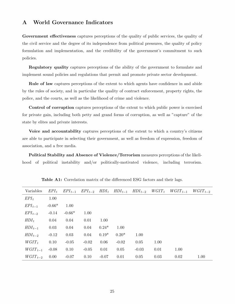
A World Governance Indicators
Government effectiveness captures perceptions of the quality of public services, the quality of
the civil service and the degree of its independence from political pressures, the quality of policy
formulation and implementation, and the credibility of the government’s commitment to such
policies.
Regulatory quality captures perceptions of the ability of the government to formulate and
implement sound policies and regulations that permit and promote private sector development.
Rule of law captures perceptions of the extent to which agents have confidence in and abide
by the rules of society, and in particular the quality of contract enforcement, property rights, the
police, and the courts, as well as the likelihood of crime and violence.
Control of corruption captures perceptions of the extent to which public power is exercised
for private gain, including both petty and grand forms of corruption, as well as ”capture” of the
state by elites and private interests.
Voice and accountability captures perceptions of the extent to which a country’s citizens
are able to participate in selecting their government, as well as freedom of expression, freedom of
association, and a free media.
Political Stability and Absence of Violence/Terrorism measures perceptions of the likeli-
hood of political instability and/or politically-motivated violence, including terrorism.
Table A1: Correlation matrix of the differenced ESG factors and their lags.
Variables EPI t EPI t−1 EPI t−2 HDI t HDI t−1 HDI t−2 WGIT t WGIT t−1 WGIT t−2
EPI t 1.00
EPI t−1 -0.66* 1.00
EPI t−2 -0.14 -0.66* 1.00
HDI t 0.04 0.04 0.01 1.00
HDI t−1 0.03 0.04 0.04 0.24* 1.00
HDI t−2 -0.12 0.03 0.04 0.19* 0.20* 1.00
WGIT t 0.10 -0.05 -0.02 0.06 -0.02 0.05 1.00
WGIT t−1 -0.08 0.10 -0.05 0.01 0.05 -0.03 0.01 1.00
WGIT t−2 0.00 -0.07 0.10 -0.07 0.01 0.05 0.03 0.02 1.00
25

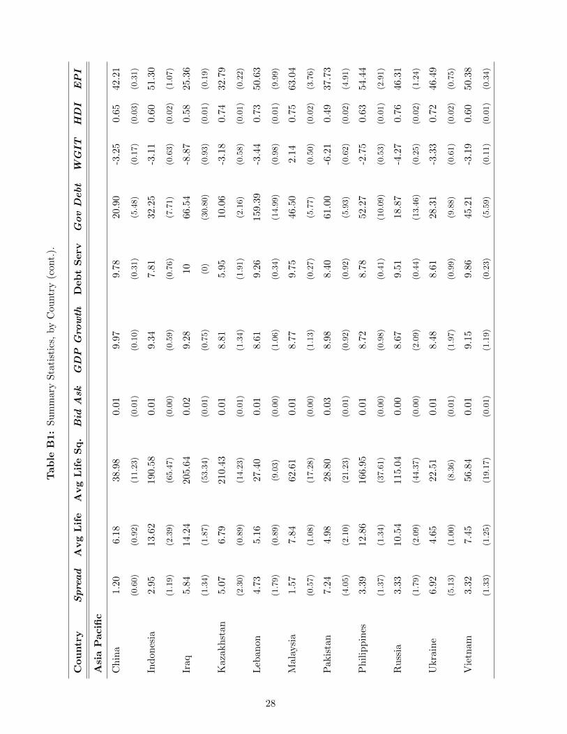
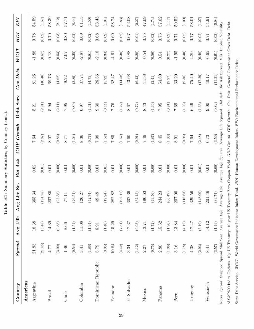
B Descriptive Statistic, by Country
26
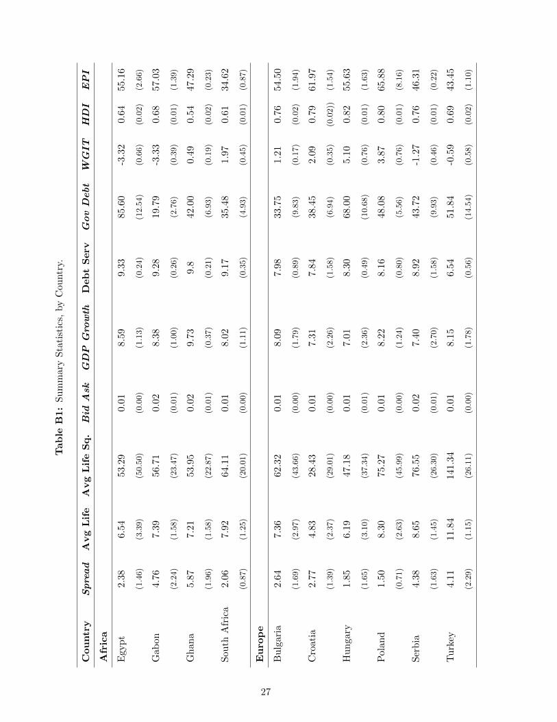
Tab
leB
1:
Su
mm
ary
Sta
tist
ics,
by
Cou
ntr
y.
Cou
ntr
ySpread
Avg
Lif
eA
vg
Lif
eS
q.
Bid
Ask
GDP
Gro
wth
Deb
tS
erv
GovDebt
WGIT
HDI
EPI
Afr
ica
Egyp
t2.3
86.
5453.
290.
018.
599.
3385
.60
-3.3
20.
6455
.16
(1.4
6)
(3.3
9)
(50.5
0)
(0.0
0)
(1.1
3)
(0.2
4)
(12.5
4)
(0.6
6)
(0.0
2)
(2.6
6)
Gab
on
4.7
67.3
956.7
10.
028.
389.
2819
.79
-3.3
30.
6857
.03
(2.2
4)
(1.5
8)
(23.4
7)
(0.0
1)
(1.0
0)
(0.2
6)
(2.7
6)
(0.3
9)
(0.0
1)
(1.3
9)
Gh
an
a5.8
77.2
153.9
50.
029.
739.
842
.00
0.49
0.54
47.2
9
(1.9
6)
(1.5
8)
(22.8
7)
(0.0
1)
(0.3
7)
(0.2
1)
(6.9
3)
(0.1
9)
(0.0
2)
(0.2
3)
Sou
thA
fric
a2.0
67.
9264.1
10.
018.
029.
1735
.48
1.97
0.61
34.6
2
(0.8
7)
(1.2
5)
(20.0
1)
(0.0
0)
(1.1
1)
(0.3
5)
(4.9
3)
(0.4
5)
(0.0
1)
(0.8
7)
Eu
rop
e
Bu
lgari
a2.6
47.
3662.3
20.
018.
097.
9833
.75
1.21
0.76
54.5
0
(1.6
9)
(2.9
7)
(43.6
6)
(0.0
0)
(1.7
9)
(0.8
9)
(9.8
3)
(0.1
7)
(0.0
2)
(1.9
4)
Cro
ati
a2.7
74.
8328.4
30.
017.
317.
8438
.45
2.09
0.79
61.9
7
(1.3
9)
(2.3
7)
(29.0
1)
(0.0
0)
(2.2
6)
(1.5
8)
(6.9
4)
(0.3
5)
(0.0
2))
(1.5
4)
Hu
nga
ry1.
856.1
947.
180.
017.
018.
3068
.00
5.10
0.82
55.6
3
(1.6
5)
(3.1
0)
(37.3
4)
(0.0
1)
(2.3
6)
(0.4
9)
(10.6
8)
(0.7
6)
(0.0
1)
(1.6
3)
Pola
nd
1.5
08.
3075.2
70.
018.
228.
1648
.08
3.87
0.80
65.8
8
(0.7
1)
(2.6
3)
(45.9
9)
(0.0
0)
(1.2
4)
(0.8
0)
(5.5
6)
(0.7
6)
(0.0
1)
(8.1
6)
Ser
bia
4.3
88.
6576.5
50.
027.
408.
9243
.72
-1.2
70.
7646
.31
(1.6
3)
(1.4
5)
(26.3
0)
(0.0
1)
(2.7
0)
(1.5
8)
(9.9
3)
(0.4
6)
(0.0
1)
(0.2
2)
Tu
rkey
4.11
11.
8414
1.3
40.
018.
156.
5451
.84
-0.5
90.
6943
.45
(2.2
9)
(1.1
5)
(26.1
1)
(0.0
0)
(1.7
8)
(0.5
6)
(14.5
4)
(0.5
8)
(0.0
2)
(1.1
0)
27
Tab
leB
1:
Su
mm
ary
Sta
tist
ics,
by
Cou
ntr
y(c
ont.
).
Cou
ntr
ySpread
Avg
Lif
eA
vg
Lif
eS
q.
Bid
Ask
GDP
Gro
wth
Deb
tS
erv
GovDebt
WGIT
HDI
EPI
Asi
aP
acifi
c
Ch
ina
1.2
06.1
838.
980.
019.
979.
7820
.90
-3.2
50.
6542
.21
(0.6
0)
(0.9
2)
(11.2
3)
(0.0
1)
(0.1
0)
(0.3
1)
(5.4
8)
(0.1
7)
(0.0
3)
(0.3
1)
Ind
on
esia
2.9
513
.62
190
.58
0.01
9.34
7.81
32.2
5-3
.11
0.60
51.3
0
(1.1
9)
(2.3
9)
(65.4
7)
(0.0
0)
(0.5
9)
(0.7
6)
(7.7
1)
(0.6
3)
(0.0
2)
(1.0
7)
Iraq
5.8
414
.24
205
.64
0.02
9.28
1066
.54
-8.8
70.
5825
.36
(1.3
4)
(1.8
7)
(53.3
4)
(0.0
1)
(0.7
5)
(0)
(30.8
0)
(0.9
3)
(0.0
1)
(0.1
9)
Kaz
akh
stan
5.0
76.
7921
0.43
0.01
8.81
5.95
10.0
6-3
.18
0.74
32.7
9
(2.3
0)
(0.8
9)
(14.2
3)
(0.0
1)
(1.3
4)
(1.9
1)
(2.1
6)
(0.5
8)
(0.0
1)
(0.2
2)
Leb
anon
4.7
35.1
627.
400.
018.
619.
2615
9.39
-3.4
40.
7350
.63
(1.7
9)
(0.8
9)
(9.0
3)
(0.0
0)
(1.0
6)
(0.3
4)
(14.9
9)
(0.9
8)
(0.0
1)
(9.9
9)
Mal
aysi
a1.5
77.
8462
.61
0.01
8.77
9.75
46.5
02.
140.
7563
.04
(0.5
7)
(1.0
8)
(17.2
8)
(0.0
0)
(1.1
3)
(0.2
7)
(5.7
7)
(0.5
0)
(0.0
2)
(3.7
6)
Pakis
tan
7.24
4.9
828
.80
0.03
8.98
8.40
61.0
0-6
.21
0.49
37.7
3
(4.0
5)
(2.1
0)
(21.2
3)
(0.0
1)
(0.9
2)
(0.9
2)
(5.9
3)
(0.6
2)
(0.0
2)
(4.9
1)
Ph
ilip
pin
es3.
3912
.86
166
.95
0.01
8.72
8.78
52.2
7-2
.75
0.63
54.4
4
(1.3
7)
(1.3
4)
(37.6
1)
(0.0
0)
(0.9
8)
(0.4
1)
(10.0
9)
(0.5
3)
(0.0
1)
(2.9
1)
Ru
ssia
3.3
310.5
411
5.04
0.00
8.67
9.51
18.8
7-4
.27
0.76
46.3
1
(1.7
9)
(2.0
9)
(44.3
7)
(0.0
0)
(2.0
9)
(0.4
4)
(13.4
6)
(0.2
5)
(0.0
2)
(1.2
4)
Ukra
ine
6.9
24.
6522.
510.
018.
488.
6128
.31
-3.3
30.
7246
.49
(5.1
3)
(1.0
0)
(8.3
6)
(0.0
1)
(1.9
7)
(0.9
9)
(9.8
8)
(0.6
1)
(0.0
2)
(0.7
5)
Vie
tnam
3.32
7.4
556
.84
0.01
9.15
9.86
45.2
1-3
.19
0.60
50.3
8
(1.3
3)
(1.2
5)
(19.1
7)
(0.0
1)
(1.1
9)
(0.2
3)
(5.5
9)
(0.1
1)
(0.0
1)
(0.3
4)
28
Tab
leB
1:
Su
mm
ary
Sta
tist
ics,
by
Cou
ntr
y(c
ont.
).
Cou
ntr
ySpread
Avg
Lif
eA
vg
Lif
eS
q.
Bid
Ask
GDP
Gro
wth
Deb
tS
erv
GovDebt
WGIT
HDI
EPI
Am
eri
cas
Arg
enti
na
21.9
318.3
836
5.34
0.02
7.64
5.21
81.2
6-1
.88
0.78
54.5
9
(21.4
8)
(5.4
8)
(194.7
5)
(0.0
1)
(2.8
7)
(2.9
1)
(40.4
6)
(0.5
7)
(0.0
2)
(1.5
7)
Bra
zil
4.7
714.
3920
7.80
0.01
8.07
5.94
68.7
30.
130.
7058
.39
(3.9
0)
(0.8
8)
(25.5
8)
(0.0
0)
(0.8
6)
(2.1
1)
(4.6
2)
(0.5
3)
(0.0
3)
(2.1
2)
Ch
ile
1.4
68.
6677
.11
0.01
8.77
7.95
9.22
7.07
0.80
57.7
1
(0.5
4)
(1.5
4)
(26.5
4)
(0.0
0)
(1.0
4)
(0.8
0)
(3.8
9)
(0.2
5)
(0.0
2)
(8.4
4)
Col
omb
ia3.
4111.
0812
6.27
0.01
8.36
6.97
37.7
4-2
.87
0.69
61.1
5
(1.8
6)
(1.9
4)
(42.7
4)
(0.0
0)
(0.7
7)
(1.3
1)
(4.7
5)
(0.8
1)
(0.0
2)
(1.5
0)
Dom
inic
anR
epu
bli
c5.7
96.
9149
.48
0.01
7.98
9.30
26.5
6-2
.18
0.68
53.4
3
(3.0
5)
(1.4
0)
(19.2
4)
(0.0
1)
(1.5
2)
(0.4
4)
(5.9
2)
(0.3
4)
(0.0
2)
(1.9
4)
Ecu
ad
or10
.84
15.
2928
2.82
0.01
7.85
7.76
32.4
7-4
.61
0.69
58.7
4
(4.4
2)
(7.3
1)
(192.1
7)
(0.0
0)
(1.6
7)
(1.2
2)
(14.5
8)
(0.3
8)
(0.0
2)
(1.8
3)
El
Salv
ador
3.34
17.
3730
2.39
0.01
7.60
8.67
43.6
8-0
.88
0.67
52.0
8
(1.1
2)
(0.9
3)
(32.1
5)
(0.0
0)
(0.9
1)
(0.7
2)
(6.4
3)
(0.2
8)
(0.0
1)
(0.2
7)
Mex
ico
2.2
713
.71
190.
630.
017.
498.
4341
.58
-0.5
40.
7547
.09
(0.7
5)
(1.7
2)
(49.5
6)
(0.0
0)
(1.8
7)
(1.3
6)
(2.4
1)
(0.5
6)
(0.0
2)
(1.7
4)
Pan
am
a2.
8015
.52
244.
230.
018.
457.
9554
.80
0.54
0.75
57.0
2
(1.0
6)
(1.9
0)
(60.4
9)
(0.0
0)
(1.3
3)
(0.9
1)
(9.9
7)
(0.2
7)
(0.0
2)
(1.1
7)
Per
u3.1
613
.84
207.
000.
018.
917.
6933
.20
-1.9
50.
7150
.52
(1.7
8)
(4.1
2)
(116.6
3)
(0.0
0)
(0.9
5)
(1.0
3)
(9.3
0)
(0.4
0)
(0.0
2)
(1.0
0)
Uru
guay
4.38
17.
4732
9.56
0.01
7.64
6.49
75.4
04.
290.
7758
.01
(2.9
3)
(5.1
9)
(148.9
0)
(0.0
1)
(2.4
8)
(1.3
3)
(17.2
9)
(0.4
8)
(0.0
2)
(1.2
7)
Ven
ezu
ela
8.4
114.
1220
1.46
0.01
6.73
9.00
40.1
7-6
.65
0.71
54.9
1
(3.5
7)
(1.4
9)
(39.7
4)
(0.0
0)
(3.5
0)
(0.8
2)
(11.3
1)
(0.9
1)
(0.0
3)
(0.9
4)
Note
s.Spread
:Str
ipp
edSpre
ad
Mid
Poin
t.Average
Life:
Aver
age
Lif
e.Average
LifeSqu
ared
:A
ver
age
Lif
eSquare
d.Bid
Ask
:B
idA
skSpre
ad.
VIX
:Im
plied
Vola
tility
of
S&
P500
Index
Opti
ons.
10y
US
Tre
asu
ry:
10
yea
rU
ST
reasu
ryZ
ero
Coup
on
Yie
ld.GDP
Growth
:G
DP
Gro
wth
.GovDebt:
Gen
eral
Gov
ernm
ent
Gro
ssD
ebt.
Deb
t
Ser
v:
Deb
tSer
vic
e.W
GIT
:W
orl
dG
over
nance
Indic
ato
rIn
dex
Tota
l.HDI:
Hum
an
Dev
elopm
ent
Index
.EPI:
Envir
onm
enta
lP
erfo
rmance
Index
.
29

Documentos de Trabajo
Banco Central de Chile
NÚMEROS ANTERIORES
La serie de Documentos de Trabajo en versión PDF
puede obtenerse gratis en la dirección electrónica:
www.bcentral.cl/esp/estpub/estudios/dtbc.
Existe la posibilidad de solicitar una copia impresa
con un costo de Ch$500 si es dentro de Chile y
US$12 si es fuera de Chile. Las solicitudes se pueden
hacer por fax: +56 2 26702231 o a través del correo
electrónico: [email protected].
Working Papers
Central Bank of Chile
PAST ISSUES
Working Papers in PDF format can be
downloaded free of charge from:
www.bcentral.cl/eng/stdpub/studies/workingpaper.
Printed versions can be ordered individually for
US$12 per copy (for order inside Chile the charge
is Ch$500.) Orders can be placed by fax: +56 2
26702231 or by email: [email protected].
DTBC – 788
Estimating Country Heterogeneity in Capital-Labor Substitution Using Panel Data
Lucciano Villacorta
DTBC – 787
Transiciones Laborales y la Tasa de Desempleo en Chile
Mario Marcel y Alberto Naudon
DTBC – 786
Un Análisis de la Capacidad Predictiva del Precio del Cobre sobre la Inflación Global
Carlos Medel
DTBC – 785
Forecasting Inflation with the Hybrid New Keynesian Phillips Curve: A Compact-
Scale Global Var Approach
Carlos Medel
DTBC – 784
Robustness in Foreign Exchange Rate Forecasting Models: Economics-Based
Modelling After the Financial Crisis
Carlos Medel, Gilmour Camelleri, Hsiang-Ling Hsu, Stefan Kania y Miltiadis
Touloumtzoglou
DTBC – 783
Desigualdad, Inflación, Ciclos y Crisis en Chile
Pablo García y Camilo Pérez

DTBC – 782
Sentiment Shocks as Drivers of Business Cycles
Agustín Arias
DTBC – 781
Precios de Arriendo y Salarios en Chile
Paulo Cox y Víctor Pérez
DTBC – 780
Pass-Through, Expectations, and Risks. What Affects Chilean Banks’ Interest Rates?
Michael Pedersen
DTBC – 779
Fiscal Policy, Sectoral Allocation, and the Skill Premium: Explaining the Decline in
Latin America’s Income Inequality
Juan Guerra-Salas
DTBC – 778
Calvo Wages vs. Search Frictions: A Horse Race in a DSGE Model of a Small Open
Economy
Markus Kirchner y Rodrigo Tranamil
DTBC – 777
Commodity Prices, Growth and Productivity: A Sectoral View
Claudia De la Huerta y Javier García-Cicco
DTBC – 776
Use of Medical Services in Chile: How Sensitive are The Results to Different
Econometric Specifications?
Alejandra Chovar, Felipe Vásquez y Guillermo Paraje
DTBC – 775
Traspaso de Tipo de Cambio a Precios en Chile: El Rol de los Insumos Importados y
del Margen de Distribución
Andrés Sansone
DTBC – 774
Calibrating the Dynamic Nelson-Siegel Model: A Practitioner Approach
Francisco Ibáñez

DOCUMENTOS DE TRABAJO • Agosto 2016