Embed Size (px)
Citation preview
DOCUMENTOS DE TRABAJO
Bank’s Lending Growth in Chile: The Role of the Senior Loan Officers Survey
Alejandro JaraJuan-Francisco MartínezDaniel Oda
N° 802 Junio 2017BANCO CENTRAL DE CHILE
BANCO CENTRAL DE CHILE
CENTRAL BANK OF CHILE
La serie Documentos de Trabajo es una publicación del Banco Central de Chile que divulga los trabajos de investigación económica realizados por profesionales de esta institución o encargados por ella a terceros. El objetivo de la serie es aportar al debate temas relevantes y presentar nuevos enfoques en el análisis de los mismos. La difusión de los Documentos de Trabajo sólo intenta facilitar el intercambio de ideas y dar a conocer investigaciones, con carácter preliminar, para su discusión y comentarios.
La publicación de los Documentos de Trabajo no está sujeta a la aprobación previa de los miembros del Consejo del Banco Central de Chile. Tanto el contenido de los Documentos de Trabajo como también los análisis y conclusiones que de ellos se deriven, son de exclusiva responsabilidad de su o sus autores y no reflejan necesariamente la opinión del Banco Central de Chile o de sus Consejeros.
The Working Papers series of the Central Bank of Chile disseminates economic research conducted by Central Bank staff or third parties under the sponsorship of the Bank. The purpose of the series is to contribute to the discussion of relevant issues and develop new analytical or empirical approaches in their analyses. The only aim of the Working Papers is to disseminate preliminary research for its discussion and comments.
Publication of Working Papers is not subject to previous approval by the members of the Board of the Central Bank. The views and conclusions presented in the papers are exclusively those of the author(s) and do not necessarily reflect the position of the Central Bank of Chile or of the Board members.
Documentos de Trabajo del Banco Central de ChileWorking Papers of the Central Bank of Chile
Agustinas 1180, Santiago, ChileTeléfono: (56-2) 3882475; Fax: (56-2) 3882231
Documento de Trabajo
N° 802
Working Paper
N° 802
BANKS’ LENDING GROWTH IN CHILE: THE ROLE OF
THE SENIOR LOAN OFFICERS SURVEY
Alejandro Jara
Banco Central de Chile
Juan-Francisco Martínez
Banco Central de Chile
Daniel Oda
Banco Central de Chile
Abstract
In order to understand the influence of banks' perceptions on their lending and thus, contribute to the
understanding of the transmission of monetary policy, we studied the role of the Senior Loan
Officers Survey (SLOS, hereafter), published quarterly by the Central Bank of Chile. The SLOS
accounts for changes in the supply of loans and factors affecting the willingness to lend, as well as
variations in the demand for credit and its motivations. By including the SLOS in the analysis, we
can go beyond the traditional determinants of credit growth rates that appear in the literature. After
controlling for macroeconomic factors and idiosyncratic characteristics of banks, we found that the
perceptions reported in the SLOS are statistically and economically significant in explaining the
dynamics of credit. This result holds for all market segments, and is robust to several specifications.
Moreover, we establish that the impact of credit standards and demand perceptions in credit growth
rates is asymmetrical and non-linear, being more significant when conditions are tightening.
Resumen
Este estudio analiza el rol de la Encuesta de Crédito Bancario (ECB), con el propósito de entender el
efecto que genera la percepción de la demanda y las políticas de otorgamiento de crédito en la
actividad crediticia, y de esta forma contribuir a una mejor comprensión de la transmisión de la
política monetaria. La ECB es publicada trimestralmente por el Banco Central de Chile y considera
los cambios en la disposición a prestar y los factores que la afectan; así como las variaciones en la
demanda de crédito y sus motivaciones. Al considerar la información contenida en la ECB en el
análisis de la dinámica del crédito bancario, y luego de controlar por factores macroeconómicos y
características idiosincráticas, encontramos que las percepciones de los bancos son estadísticamente
y económicamente significativas. Este resultado es válido para todos los segmentos del crédito y es
robusto a varias especificaciones. Además, se encuentra que los estándares de crédito y las
percepciones sobre la demanda tienen un efecto asimétrico y no lineal sobre las tasas de crecimiento
del crédito bancario, siendo más significativos cuando las condiciones se vuelven más restrictivas.
We are grateful to Claudio Raddatz and colleagues in the Financial Policy Division at the Central Bank of Chile for their
helpful comments at different stages of this research. The opinions expressed in this article are the authors’ own and do not
necessarily represent the views of the Central Bank of Chile or its Board Members. The usual disclaimer applies. Emails:
1 Introduction and motivation
A key issue in macroeconomics is to understand the transmission mechanisms of monetary
policy into the real economy. Although there is consensus about the non-neutrality of
monetary policy in the short run (Bernanke and Gertler, 1995), there is less agreement
about the channels through which monetary policy is transmitted. As a response arises
the credit channel, composed by the interaction between the balance sheet channel and
its bank lending component. The balance sheet channel is associated with the e�ects of
interest rates on agents' balance-sheets and income statements, making it closely related
to credit demand. In turn, the bank lending channel is associated with the implications of
monetary policy on banks' willingness to lend and therefore it relates with credit supply.
Although important, this framework is still debateable, mainly because of the di�culties
encompassed in disentangling demand and supply in�uences on credit growth rates. This
is where the more recent literature frames the use of Senior Loans O�cers' Surveys (SLOS)
on lending standards and demand perceptions, in their power to help to identify credit
dynamics and their determinants.
Changes in lending standards contained in SLOS are key to understanding credit dy-
namics because they re�ect banks' expectations about the economy and the risks faced by
the banking sector. As such, they help to address one of the most challenging aspects of the
credit channel, namely the magnitudes and directions of the bank lending component and
its e�ects on the real economy.1 Along these lines, Ciccarelli et al. (2011) emphasizes that
the capacity of SLOS in disentangling demand and supply factors behind credit growth
rates relies precisely on the possibility to capture banks' expectations.
The empirical evidence shows that lending standards contained in SLOS help to identify
the bank lending channel and, consequently, to understand the overall role of the credit
channel in the transmission of monetary policy. In fact, changes in lending standards have
been linked to changes in credit growth rates and interest rates (Berg et al, 2005; Bell and
Pugh, 2014). By the same token, provided that credit supply shifts, loosening in lending
standards has been associated with excessive credit growth rates and higher delinquency
rates (Keeton, 1999). Moreover, there is evidence that the credit channel tends to amplify
the monetary policy e�ects on output and in�ation and that the strictness in credit stan-
dards for mortgage loans observed during the sub-prime crisis reduced economic activity
1The balance sheet channel, on the other hand, is relatively simpler to address, since it relates to theinterest rate e�ects on the agents' budget constraints and its e�ects on spending.
1
(Ciccarelli et al., 2011). Finally, there is also evidence that lending standards outperform
other variables �in particular risk metrics�in determining real activity (Waters, 2012),
and that a subset of banks' perceptions are able to reasonably predict credit growth and
interest rates one quarter ahead (Bell and Pugh, 2014).
Despite the evidence supporting the relevance of lending standards at the aggregate
level, their contribution at the sectorial level is less conclusive. For instance, Cunninham
(2006) shows that the disaggregation of lending standards at di�erent market segments (e.g
mortgage, commercial, consumer) helps to explain the dynamics of real activity in the US,
but not the credit growth rates in those speci�c segments. On the �ip side, Del Giovane
et al. (2011) focus on the corporate sector to show that banks' perceptions about �rms'
risk, jointly with their level of capital adequacy, played an important role with respect to
changes in the credit supply during the sub-prime crisis. Additionally, Basset el al. (2014)
by the means of the US SLOS, construct an index of credit supply based on the survey's
information on household and corporate loans. They �nd that, after controlling for speci�c
banks' characteristics and macro variables, the index of credit supply, when tightened, can
explain lower demand for credit and the ease of monetary policy.
Credit market equilibrium depends not only on the supply of credit, but also on the
demand. While macroeconomic factors, such as GDP growth and interest rates, can closely
track aggregate demand for credit, SLOS can provide valuable information about banks'
perception of credit demand. For example, Breeden and Canals-Cerdá (2016) use the US
SLOS to identify periods of high demand for credit. They �nd that periods of high demand
correspond to low-risk cohorts of borrowers and periods of low demand correspond to high-
risk vintages. Therefore, by considering demand-side factors, like the ability and willingness
to consume and invest, the authorities can improve their assessment of loan performance.
At the policy level, central banks use the insights embedded in SLOS, such as banks'
willingness to lend and their perceptions about credit demand, when making decisions
about interest rates and other types of policies. In fact, SLOS helps them to disentangle
the mechanisms behind the monetary policy transmission and to better understand and
regulate credit markets. Since banks can in�uence credit cycles through their forward-
looking decisions on loan-loss provisioning (Balasubramanyan et al., 2014), their behavior
generates a feedback e�ect on lending standards, lending activity, and output (Lown et al.,
2000, 2006).
In Chile, the SLOS surveys top bank o�cials since 2003 on a quarterly basis, providing
qualitative information regarding the banks' willingness to lend (changes in lending stan-
2
dards) and their perception about the demand for credit. The Chilean SLOS asks about
banks' opinions on di�erent market segments (commercial, consumer, mortgage, construc-
tion), comparing current lending standards with the standards of the previous quarter. The
SLOS in Chile also provides answers to the causes that may be underlying banks' decisions
to change their lending standards (e.g. macroeconomic environment, banks' capital, fund-
ing conditions). It also asks about the speci�c conditions that may be a�ecting lending
standards (e.g. credit lines, spreads, collateral).2 As shown in Calani et al. (2010), the
SLOS can be used as a reasonable instrument to address the identi�cation problem faced
traditionally in panel estimations of bank credit growth rates in Chile.
Aside from Calani et al. (2010)'s contribution, there have been few attempts to un-
derstand what drives credit dynamics based on credit standards and banks' perceptions in
Chile. In this paper we �ll this gap by studying the role played by the Chilean SLOS in
understanding banks' lending growth rates during the 2003q1-2015q3 sample period. We
�nd that, after controlling for macroeconomic factors and banks' balance sheet character-
istics, the SLOS add valuable information to the dynamic of bank lending. In particular,
we �nd that changes in lending standards have a stronger impact than changes in demand
perceptions. These results are valid for all market segments (commercial, consumer, and
mortgage) and are robust to di�erent speci�cations. Moreover, we �nd that the impact
of the SLOS on credit growth rates is asymmetric and non-linear, being more signi�cant
when conditions are tightening.
The paper is organized as follows. Section 2 brie�y describes the structure of the
Chilean SLOS and its main aggregate results since it was �rst released. It emphasizes the
need to go beyond the aggregate behavior of the SLOS in order to avoid the aggregation
bias resulting from the heterogeneous responses at the bank level. Section 3 describes the
empirical strategy used to address the role of the SLOS in lending growth rates. It presents
di�erent speci�cations aimed to account for the persistence in the SLOS responses. Section
4 addresses the issue of asymmetry and non-linearity. Section 5 concludes.
2 The Chilean SLOS
The Chilean SLOS or "Encuesta de Crédito Bancario" (ECB), quarterly surveys senior
managers of commercial banks in Chile since earlier 2003. The main purpose of this survey
is to assess demand and supply factors a�ecting the dynamic of banks' lending growth
2See Jara and Silva (2007) for a more detailed description of the Chilean SLOS.
3
rates. The survey is used to get a better understanding about the transmission of monetary
policy, as well as the potential �nancial risks associated with changes in the behavior of
banks. Supply-side conditions are measured by changes in the banks' willingness to lend,
while demand-side factors are measured by changes in the banks' perception about credit
demand. In addition, the survey allows to identify the reasons behind those changes and,
in the case of supply conditions, it allows to identify the speci�c factors re�ecting such
conditions.
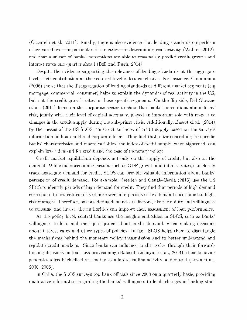
Note: The LHS panel shows banks' changes in their willingness to lend. A positive (negative) numbermeans that banks have loosened (tightened) their lending conditions compared to the previous quarter. TheRHS panel shows banks' perception about demand for credit. A positive (negative) number means thatthe perception of banks is that the demand is stronger (weaker) compared to the previous quarter. Source:Authors' calculations based on the Chilean Senior Loan O�cers Survey, Central Bank of Chile.
Figure 1: Lending conditions and demand perception for corporate
loans
The Chilean SLOS asks speci�cally about how lending conditions have changed com-
pared to the previous quarter. Senior o�cers have to choose between �ve options, de-
pending on whether lending conditions have become: (i) strongly loosened, (ii) moderately
loosened, (iii) unchanged, (iv) moderately tightened, or (v) strongly tightened. As for
credit demand, they are asked about their perception compared to the previous quarter,
having to choose also between �ve options, depending on whether their perception is that
the demand for credit is: (i) strongly higher, (ii) moderately higher, (iii) unchanged, (iv)
moderately weaker, or (v) strongly weaker.
4
Figure 1 shows the aggregate results of lending conditions and demand perceptions in
the corporate market segment (i.e commercial loans to large �rms). Positive numbers are
associated with loose lending standards and higher demand perceptions, while negative
numbers are associated otherwise. The answers for both, lending conditions and demand
perceptions are mapped into the 1.5 and -1.5 range in order to be able to distinguish strong
from moderate answers. Although it is a common practice in the literature to equally
weight moderate and strong changes in supply conditions and demand perceptions, in Chile
stronger changes have a greater impact on credit growth rates than moderate changes.3
Figure 1 also shows the aggregate index constructed from the unweighted answers (simple
average) and the index constructed after weighting the responses by the banks' speci�c
market share.4
In Chile, lending conditions were moderately loose before 2007, but became tightened
and strongly tightened during the Global Financial Crisis (GFC, hereafter). Since then,
banks increased their willing to lend for a short period, but less so by the end of the sample
period. Demand perceptions followed a similar cyclical pattern than lending conditions,
however they fell less dramatically during the GFC. Moreover, demand perceptions showed
a persistent, although moderate, decreased since late 2012, something that was less pro-
nounced in the supply conditions. In addition, there has been higher discrepancy between
weighted and unweighted values for demand perceptions than for credit standards, which
suggests a higher heterogeneity in this component.
Figure 2 shows the factors behind the change in banks' willingness to lend and the factors
that banks consider are behind the changes in the demand for credit. On average, banks
argue that the economic conditions, as well as the riskiness of their portfolio, are the most
relevant factors that explain their changes in lending conditions. Meanwhile, idiosyncratic
factors, such as the level of capital and the funding conditions, have not played a signi�cant
role in explaining banks' willingness to lend in Chile. On the other hand, all factors behind
the changes observed in demand perceptions play some role. Nonetheless, when the demand
for commercial loans was perceived to be weaker �as it was during the GFC and during the
last two years of the sample�it was because investments and acquisitions fell, and less so
because there were changes in the need for working capital or in the degree of substitution
from other sources of credit.
3For a further discussion on this issue see Section 4.4The distinction between weighted and unweighted aggregate indexes is, in principle, relevant in Chile
because banks' sizes are very heterogeneous.
5
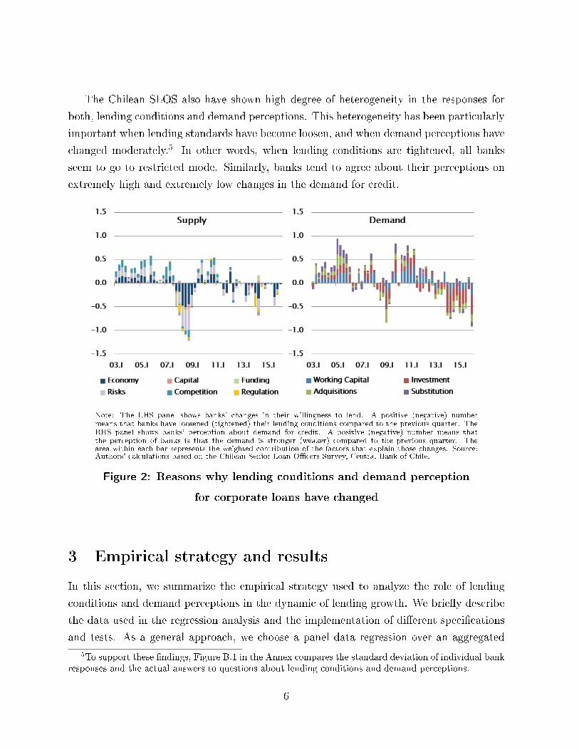
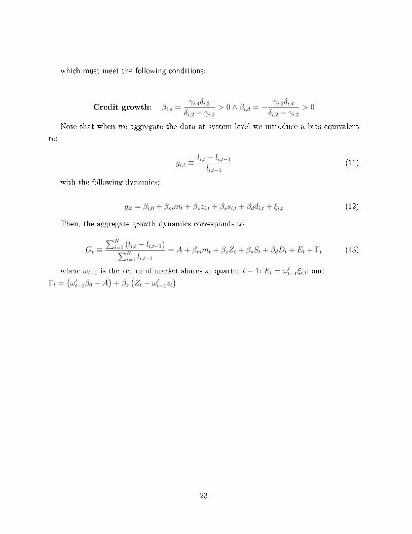
The Chilean SLOS also have shown high degree of heterogeneity in the responses for
both, lending conditions and demand perceptions. This heterogeneity has been particularly
important when lending standards have become loosen, and when demand perceptions have
changed moderately.5 In other words, when lending conditions are tightened, all banks
seem to go to restricted mode. Similarly, banks tend to agree about their perceptions on
extremely high and extremely low changes in the demand for credit.
Note: The LHS panel shows banks' changes in their willingness to lend. A positive (negative) numbermeans that banks have loosened (tightened) their lending conditions compared to the previous quarter. TheRHS panel shows banks' perception about demand for credit. A positive (negative) number means thatthe perception of banks is that the demand is stronger (weaker) compared to the previous quarter. Thearea within each bar represents the weighted contribution of the factors that explain those changes. Source:Authors' calculations based on the Chilean Senior Loan O�cers Survey, Central Bank of Chile.
Figure 2: Reasons why lending conditions and demand perception
for corporate loans have changed
3 Empirical strategy and results
In this section, we summarize the empirical strategy used to analyze the role of lending
conditions and demand perceptions in the dynamic of lending growth. We brie�y describe
the data used in the regression analysis and the implementation of di�erent speci�cations
and tests. As a general approach, we choose a panel data regression over an aggregated
5To support these �ndings, Figure B.1 in the Annex compares the standard deviation of individual bankresponses and the actual answers to questions about lending conditions and demand perceptions.
6
regression at the banking system level for various reasons. First, because this approach takes
into account the heterogeneity described above, increases the sample size, and enhances
the statistical properties. Additionally, because this type of speci�cation allows us to avoid
aggregation biases.6
3.1 The data
Our empirical approach relies on the combination of several datasets. First, we use the
SLOS information for 10 individual banks regarding their changes in lending standards
and their perception of credit demand in di�erent market segments (commercial, consumer,
mortgage) published quarterly by the Central Bank of Chile (CBC).7 Second, we construct
a dataset of credit growth rates and other banks' characteristics based on balance sheet
information published by the Superintendency of Banks and Financial Institutions (SBIF).
Our dataset speci�cally deals with the issue of mergers and acquisitions in the traditional
fashion.8 Finally, we use a set of aggregate macroeconomic and �nancial variables from the
CBC that might a�ect either the demand for credit or the willingness to lend by bankers.9
As explained above, extreme alternatives given in the survey for supply conditions and
demand perceptions are weighted more than moderated changes. In particular, we de�ne
the lending conditions for each bank b at time t as Lcbt, such that:
Lcbt =
1.5 if lending standards are strongly loosened
1.0 if lending standards are moderately loosened
0 if lending standards are unchanged
−1.0 if lending standards are moderately tightened
−1.5 if lending standards are strongly tightened
(1)
In general, tighter lending standards can take the form of higher spreads, smaller lines
of credit, or the requirement to provide better collateral. These changes are the result of
6See Appendix A for further details on the aggregation bias.7We focus our empirical analysis on these 10 banks because they responded the SLOS in the three
market segments and they responded the survey during the entire sample period. In addition, these 10banks account for 94% of the total credit.
8Speci�cally, if a currently active bank is the result of a merger or acquisition in the past, we constructa �ctitious bank for the period before the merger was e�ective as in Avanzini and Jara (2015).
9See Table C3 in the Appendix.
7
banks' general perception about credit risk, funding conditions, and the level of capital.
In a similar fashion, we de�ne the demand perception for each bank b and time t as Dpbt,
such that:
Dpbt =
1.5 if demand is strongly higher
1.0 if demand is moderately higher
0 if demand is unchanged
−1.0 if demand is moderately weaker
−1.5 if demand is strongly weaker
(2)
The survey also asks about the reasons why banks think that their perception about
the demand has changed (liquidity needs, competition, among others).
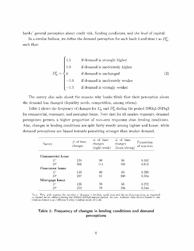
Table 1 shows the frequency of changes for Lcbt and D
pbt during the period 2003q1-2015q3
for commercial, consumer, and mortgage loans. Note that for all market segments, demand
perceptions present a higher proportion of non-zero responses than lending conditions.
Also, changes in lending conditions are split fairly evenly among tighter and looser, while
demand perceptions are biased towards perceiving stronger than weaker demand.
Survey# of timechanges
# of timechanges(tight/weak)
# of timechanges(loose/strong)
Proportionof non-zero
Commercial loans
Lc 176 90 86 0.352Dp 308 114 194 0.616
Consumer loans
Lc 148 80 68 0.296Dp 297 97 200 0.594
Mortgage loans
Lc 136 70 66 0.272Dp 272 78 194 0.544
Note: This table reports the number of changes in lending conditions and demand perceptions, as reportedby banks' senior o�cers during the 2003q1-2015q3 sample period. Source: Authors' calculations based on theChilean Senior Loan O�cers Survey, Central Bank of Chile.
Table 1: Frequency of changes in lending conditions and demandperceptions
8
3.2 Regression analysis
To con�gure the baseline regression speci�cation we follow conventional microeconomic
theory adapted to the credit market. In essence, to identify the relationship between credit
growth rates and its determinants we need to combine macroeconomic factors, idiosyncratic
banks' characteristics and the instruments that account separately for demand and supply
shifts.10 This is where we recourse to the use of the Chilean SLOS. After de�ning the
demand for and supply of credit we determine the following credit growth equation for
each bank unit:
∆Yb,t = α0 + α1Xt + α2Xb,t−1 + α3Lcbt + α4D
pbt + fb + εb,t (3)
where ∆Yb,t is the quarterly log change in domestic lending of bank b at time t. Xt
represents the contemporaneous macroeconomic factors, including GDP growth and the
domestic interest rates. Xb,t−1 represent the one-quarter lagged vector of idiosyncratic
banks' characteristics, including size, capital adequacy ratio, deposits to total assets and
the liquidity ratio. Lcbt andD
pbt represent banks' lending conditions and demand perceptions,
and fb represents banks' �xed e�ects.11
In our baseline regression of equation (3), lending conditions and demand perceptions
are included in levels. However, following Del Giovane et al (2011) and in order to take
into account the role of persistency in the SLOS's responses, we also include the cumulative
changes of these variables in alternative speci�cations to equation (3). In fact, according to
Del Giovane et al (2011) there should be a rigorous consideration about the persistence of
lending standards and demand perceptions when studying their potential a�ect on credit
growth rates. Lending standards may vary in an infrequent manner, making the e�ect of one
speci�c change in lending standards be insigni�cant on credit growth rates (i.e. one swallow
does not make summer). However, if these infrequent variations are aggregated through
time, they could in�uence credit activity. Put di�erently, if cumulative credit rejections
grow steadily, this makes a case for determining credit growth variations. However, the
argument for accumulating changes in demand perception is less strong, because these
changes are by nature more persistent, due to the learning process about the states of
nature that characterize borrowers' behavior (Milani, 2007).
10Appendix A describes the simple conceptual framework underlying in the identi�cation of supply anddemand factors.
11See Table C4 in the Appendix for the de�nition of these variables.
9
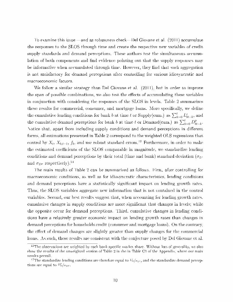
To examine this issue �and as robustness check�Del Giovane et al. (2011) accumulate
the responses to the SLOS through time and create the respective new variables of credit
supply standards and demand perceptions. These authors test the simultaneous accumu-
lation of both components and �nd evidence pointing out that the supply responses may
be informative when accumulated through time. However, they �nd that such aggregation
is not satisfactory for demand perceptions after controlling for various idiosyncratic and
macroeconomic factors.
We follow a similar strategy than Del Giovane et al. (2011), but in order to improve
the span of possible combinations, we also test the e�ects of accumulating these variables
in conjunction with considering the responses of the SLOS in levels. Table 2 summarizes
these results for commercial, consumer, and mortgage loans. More speci�cally, we de�ne
the cumulative lending conditions for bank b at time t or Supply(cum.) as∑t
k=0 Lcbt−k, and
the cumulative demand perceptions for bank b at time t or Demand(cum.) as∑t
k=0Dpbt−k.
Notice that, apart from including supply conditions and demand perceptions in di�erent
forms, all estimations presented in Table 2 correspond to the weighted OLS regressions that
control by Xt, Xb,t−1, fb, and use robust standard errors.12 Furthermore, in order to make
the estimated coe�cients of the SLOS comparable in magnitude, we standardize lending
conditions and demand perceptions by their total (time and bank) standard deviation (σLc
and σDp respectively).13
The main results of Table 2 can be summarized as follows. First, after controlling for
macroeconomic conditions, as well as for idiosyncratic characteristics, lending conditions
and demand perceptions have a statistically signi�cant impact on lending growth rates.
Thus, the SLOS variables aggregate new information that is not contained in the control
variables. Second, our best results suggest that, when accounting for lending growth rates,
cumulative changes in supply conditions are more signi�cant that changes in levels; while
the opposite occur for demand perceptions. Third, cumulative changes in lending condi-
tions have a relatively greater economic impact on lending growth rates than changes in
demand perceptions for households credit (consumer and mortgage loans). On the contrary,
the e�ect of demand changes are slightly greater than supply changes for the commercial
loans. As such, these results are consistent with the conjecture posed by Del Giovane et al.
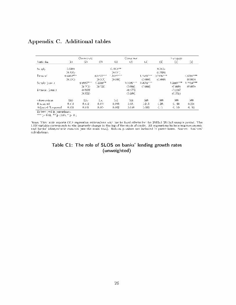
12The observations are weighted by each bank speci�c market share. Without loss of generality, we alsoshow the results of the unweighted version of Table 2 in the in Table C1 of the Appendix, where our mainresults prevail.
13The standardize lending conditions are therefore equal to Lcbt/σLc , and the standardize demand percep-
tions are equal to Dpbt/σDp .
10
Commercial Consumer MortgageVariables (1) (2) (3) (1) (2) (3) (1) (2) (3)
Supply 0.2089 0.2522 0.0049(0.216) (0.155) (0.964)
Demand 0.7693*** 0.7630*** 0.9074*** 0.9577*** 0.3258*** 0.2866***(0.000) (0.000) (0.000) (0.000) (0.006) (0.008)
Supply (cum.) 0.8370*** 0.5927** 1.6160*** 1.5100*** 1.4844*** 1.3031***(0.002) (0.022) (0.002) (0.003) (0.000) (0.000)
Demand (cum.) -0.2073 -0.1299 -0.2605(0.336) (0.569) (0.237)
Observations 500 500 500 500 500 500 500 500 500R-squared 0.190 0.152 0.195 0.256 0.220 0.288 0.154 0.196 0.206Adjusted R-squared 0.160 0.120 0.165 0.228 0.191 0.261 0.122 0.166 0.177
Robust pval in parentheses*** p<0.01, ** p<0.05, * p<0.1
Note: This table reports OLS regression estimates with banks �xed e�ects for the 2003q1-2015q3 sample period. TheLHS variable corresponds to the quarterly change in the log of the stock of credit. All regressions include macroeconomicand banks' idiosyncratic controls (see the main text). Additionally, observations are weighted by the respective marketshare, and robust p-values are included in parentheses. Source: Authors' calculations.
Table 2: The role of SLOS on banks' lending growth rates
(2011), in the sense that a persistent change in lending conditions is required to have an
impact on credit growth rates. However, for demand perceptions, our results show that no
accumulation is required, as perceptions in levels are signi�cant in explaining credit growth
rates in all market segments.
3.3 Addressing collinearity
One issue that need further attention is the potential collinearity that might exist between
supply and demand conditions, and between these conditions and the macroeconomic and
idiosyncratic controls included in equation (3); and how this potential collinearity might
a�ect our previous �ndings.
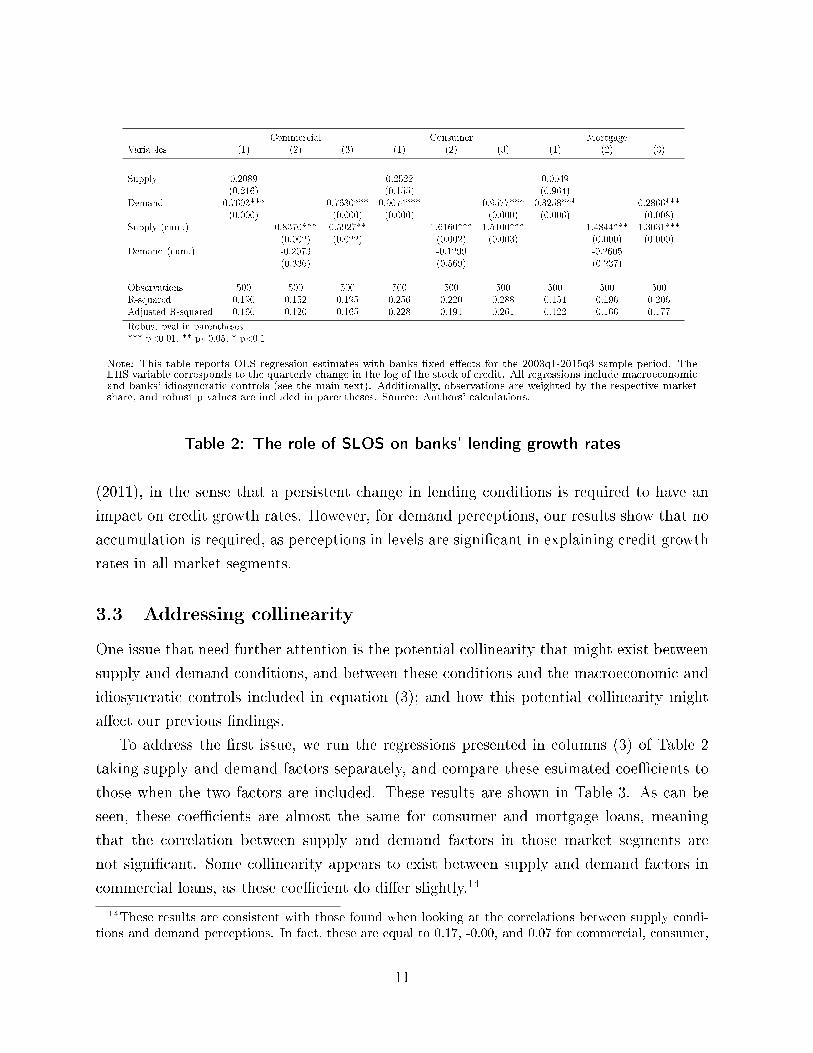
To address the �rst issue, we run the regressions presented in columns (3) of Table 2
taking supply and demand factors separately, and compare these estimated coe�cients to
those when the two factors are included. These results are shown in Table 3. As can be
seen, these coe�cients are almost the same for consumer and mortgage loans, meaning
that the correlation between supply and demand factors in those market segments are
not signi�cant. Some collinearity appears to exist between supply and demand factors in
commercial loans, as these coe�cient do di�er slightly.14
14These results are consistent with those found when looking at the correlations between supply condi-tions and demand perceptions. In fact, these are equal to 0.17, -0.00, and 0.07 for commercial, consumer,
11
Commercial Consumer MortgageVariables (1) (2) (3) (1) (2) (3) (1) (2) (3)
Supply (cum.) 0.8117*** 0.5927** 1.5955*** 1.5100*** 1.3501*** 1.3031***(0.002) (0.022) (0.002) (0.003) (0.000) (0.000)
Demand 0.8109*** 0.7630*** 0.9863*** 0.9577*** 0.3269*** 0.2866***(0.000) (0.000) (0.000) (0.000) (0.005) (0.008)
Observations 500 500 500 500 500 500 500 500 500R-squared 0.150 0.187 0.195 0.220 0.252 0.288 0.193 0.154 0.206Adjusted R-squared 0.120 0.159 0.165 0.192 0.226 0.261 0.164 0.124 0.177Robust pval in parentheses*** p<0.01, ** p<0.05, * p<0.1
Note: This table reports OLS regression estimations with banks �xed e�ects for the 2003q1-2015q3 sample period. TheLHS variable corresponds to the quarterly change in the log of the stock of credit. All regressions include macroeconomicand banks' idiosyncratic controls (see the main text). Additionally, observations are weighted by the respective marketshare, and robust p-values are included in parentheses. Source: Authors' calculations.
Table 3: The role of SLOS on banks' lending growth rates
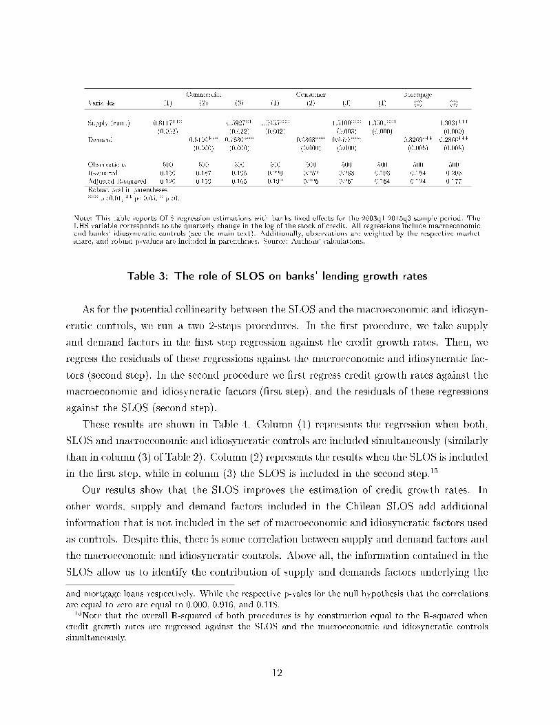
As for the potential collinearity between the SLOS and the macroeconomic and idiosyn-
cratic controls, we run a two 2-steps procedures. In the �rst procedure, we take supply
and demand factors in the �rst step regression against the credit growth rates. Then, we
regress the residuals of these regressions against the macroeconomic and idiosyncratic fac-
tors (second step). In the second procedure we �rst regress credit growth rates against the
macroeconomic and idiosyncratic factors (�rst step), and the residuals of these regressions
against the SLOS (second step).
These results are shown in Table 4. Column (1) represents the regression when both,
SLOS and macroeconomic and idiosyncratic controls are included simultaneously (similarly
than in column (3) of Table 2). Column (2) represents the results when the SLOS is included
in the �rst step, while in column (3) the SLOS is included in the second step.15
Our results show that the SLOS improves the estimation of credit growth rates. In
other words, supply and demand factors included in the Chilean SLOS add additional
information that is not included in the set of macroeconomic and idiosyncratic factors used
as controls. Despite this, there is some correlation between supply and demand factors and
the macroeconomic and idiosyncratic controls. Above all, the information contained in the
SLOS allow us to identify the contribution of supply and demands factors underlying the
and mortgage loans respectively. While the respective p-vales for the null hypothesis that the correlationsare equal to zero are equal to 0.000, 0.916, and 0.118.
15Note that the overall R-squared of both procedures is by construction equal to the R-squared whencredit growth rates are regressed against the SLOS and the macroeconomic and idiosyncratic controlssimultaneously.
12
dynamic of credit growth rates. Moreover, and the overall relative signi�cance of supply
conditions and demand perceptions remain the same than previously found in every market
segment.
Commercial Consumer MortgageVariables (Simult.) (First) (Second) (Simult.) (First) (Second) (Simult.) (First) (Second)
(1) (2) (3) (1) (2) (3) (1) (2) (3)
Supply (cum.) 0.5927** 0.8295*** 0.3983* 1.5100*** 1.2213** 1.1625** 1.3031*** 1.1952*** 0.9591***(0.022) (0.001) (0.087) (0.003) (0.017) (0.017) (0.000) (0.000) (0.000)
Demand 0.7630*** 0.7660*** 0.5948*** 0.9577*** 1.2161*** 0.6795*** 0.2866*** 0.3604*** 0.2590**(0.000) (0.000) (0.000) (0.000) (0.000) (0.000) (0.008) (0.002) (0.015)
Observations 500 500 500 500 500 500 500 500 500R-squared 0.195 0.195 0.195 0.288 0.288 0.288 0.206 0.206 0.206Adjusted R-squared 0.165 0.165 0.165 0.261 0.261 0.261 0.177 0.177 0.177
Robust pval in parentheses*** p<0.01, ** p<0.05, * p<0.1
Note: Column (1) represents the regression when both, SLOS and macroeconomic and idiosyncratic controls are includedsimultaneously (similarly than in column (3) of Table 2). Column (2) represents the results when the SLOS is includedin the �rst step, where in column (3) the SLOS is included in the second step (see the main text for more details).Additionally, observations are weighted by the respective market share, and robust p-values are included in parentheses.Source: Authors' calculations.
Table 4: The role of SLOS on banks' lending growth rates
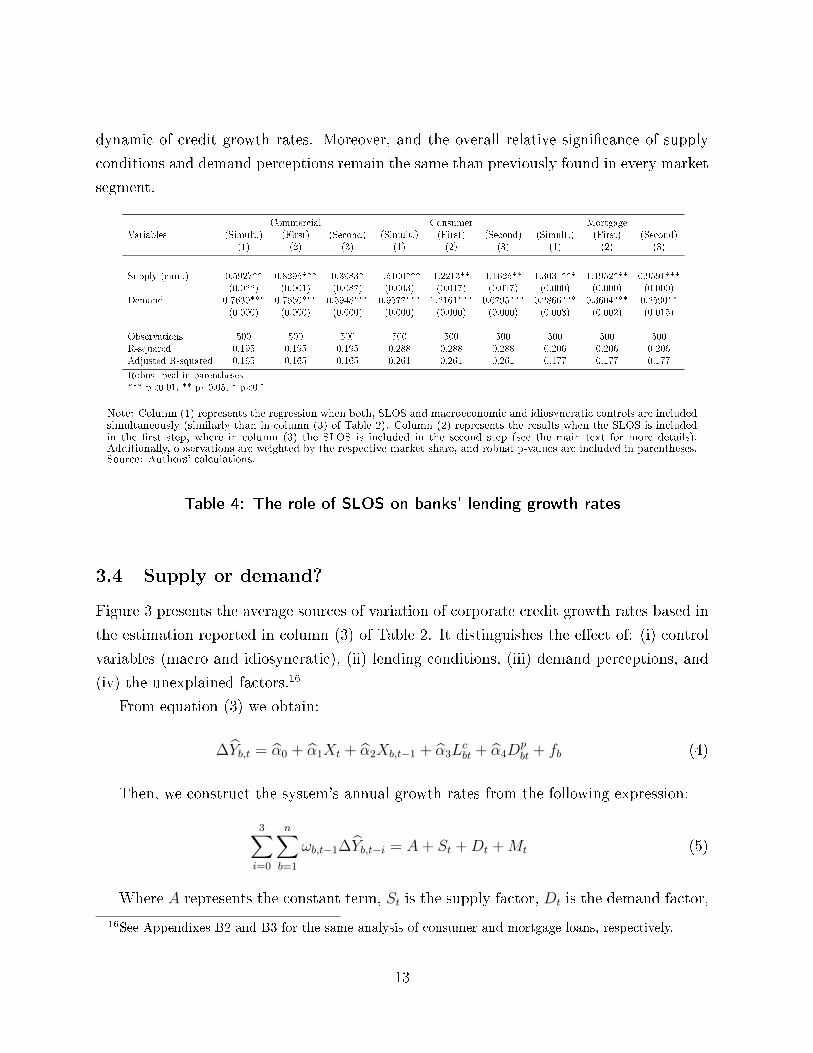
3.4 Supply or demand?
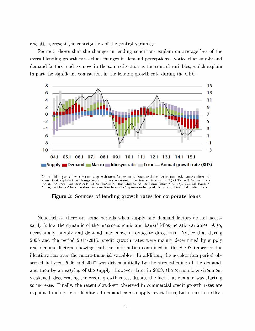
Figure 3 presents the average sources of variation of corporate credit growth rates based in
the estimation reported in column (3) of Table 2. It distinguishes the e�ect of: (i) control
variables (macro and idiosyncratic), (ii) lending conditions, (iii) demand perceptions, and
(iv) the unexplained factors.16
From equation (3) we obtain:
∆Yb,t = α0 + α1Xt + α2Xb,t−1 + α3Lcbt + α4D
pbt + fb (4)
Then, we construct the system's annual growth rates from the following expression:
3∑i=0
n∑b=1
ωb,t−1∆Yb,t−i = A+ St +Dt +Mt (5)
Where A represents the constant term, St is the supply factor, Dt is the demand factor,
16See Appendixes B2 and B3 for the same analysis of consumer and mortgage loans, respectively.
13
and Mt represent the contribution of the control variables.
Figure 3 shows that the changes in lending conditions explain on average less of the
overall lending growth rates than changes in demand perceptions. Notice that supply and
demand factors tend to move in the same direction as the control variables, which explain
in part the signi�cant contraction in the lending growth rate during the GFC.
Note: This �gure shows the annual growth rates for corporate loans and the factors (controls, supply, demand,error) that explain that change according to the regression estimated in column (3) of Table 2 for corporateloans. Source: Authors' calculations based on the Chilean Senior Loan O�cers Survey, Central Bank ofChile, and banks' balance sheet information from the Superintendency of Banks and Financial Institutions.
Figure 3: Sources of lending growth rates for corporate loans
Nonetheless, there are some periods when supply and demand factors do not neces-
sarily follow the dynamic of the macroeconomic and banks' idiosyncratic variables. Also,
occasionally, supply and demand may move in opposite directions. Notice that during
2005 and the period 2014-2015, credit growth rates were mainly determined by supply
and demand factors, showing that the information contained in the SLOS improved the
identi�cation over the macro-�nancial variables. In addition, the acceleration period ob-
served between 2006 and 2007 was driven initially by the strengthening of the demand,
and then by an easying of the supply. However, later in 2009, the economic environment
weakened, decelerating the credit growth rates, despite the fact that demand was starting
to increase. Finally, the recent slowdown observed in commercial credit growth rates are
explained mainly by a debilitated demand, some supply restrictions, but almost no e�ect
14
of macro-�nancial factors.
Supply Demand Macro Idiosyncratic R2
Commercial 20.9 30.7 26.7 21.7 0.1952003-2006 23.4 21.4 24.8 30.4 0.3482007-2012 27.5 26.3 26.1 20.0 0.2852012-2015 15.5 20.7 21.7 42.1 0.326
Consumer 11.9 37.9 24.8 25.5 0.2882003-2006 14.8 10.8 20.7 53.7 0.2292007-2012 15.7 35.0 29.6 19.8 0.4972012-2015 22.2 22.7 25.7 29.3 0.444
Mortgage 29.3 20.5 23.6 26.5 0.2062003-2006 17.6 17.6 22.8 41.9 0.3112007-2012 34.6 21.3 20.4 23.7 0.5372012-2015 21.5 23.0 21.9 33.6 0.610
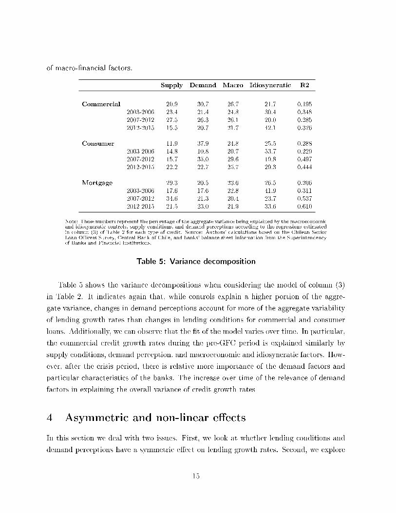
Note: These numbers represent the percentage of the aggregate variance being explained by the macroeconomicand idiosyncratic controls, supply conditions, and demand perceptions according to the regressions estimatedin column (3) of Table 2 for each type of credit. Source: Authors' calculations based on the Chilean SeniorLoan O�cers Survey, Central Bank of Chile, and banks' balance sheet information from the Superintendencyof Banks and Financial Institutions.
Table 5: Variance decomposition
Table 5 shows the variance decompositions when considering the model of column (3)
in Table 2. It indicates again that, while controls explain a higher portion of the aggre-
gate variance, changes in demand perceptions account for more of the aggregate variability
of lending growth rates than changes in lending conditions for commercial and consumer
loans. Additionally, we can observe that the �t of the model varies over time. In particular,
the commercial credit growth rates during the pre-GFC period is explained similarly by
supply conditions, demand perception, and macroeconomic and idiosyncratic factors. How-
ever, after the crisis period, there is relative more importance of the demand factors and
particular characteristics of the banks. The increase over time of the relevance of demand
factors in explaining the overall variance of credit growth rates
4 Asymmetric and non-linear e�ects
In this section we deal with two issues. First, we look at whether lending conditions and
demand perceptions have a symmetric e�ect on lending growth rates. Second, we explore
15
if there is any evidence of non-linearity, i.e whether strong changes in SLOS have a more
di�erentiated impact on lending growth rates than moderate changes. In both cases, we
use as the baseline regression speci�cation the one presented in column (3) of Table 2, for
each type of credit (commercial, consumer, and mortgage). Notice that, in order to avoid
over-parametrization, we compiled the variables under analysis in two separate groups.17
The asymmetric e�ect is captured by estimating the following equation:
∆Yb,t = β0 + β1Xt + β2Xb,t−1 + (6)
β3cumLloosenedbt + β4cumL
tightenedbt + β5D
higherbt + β6D
weakerbt + fb + εb,t
where Llossenedbt takes the value of +1 when lending conditions are more �exible, and 0
otherwise. Similarly, Ltighterbt takes the value of -1 when lending conditions are tightening,
and 0 otherwise. Then, we compute the cumulative e�ect for both variables (cumLloosenedbt
and cumLtighterbt , respectively), in the same fashion as explained above. For demand per-
ceptions we follow the same method, Dhigherbt takes value of +1 when it is stronger, and 0
otherwise; while Dweakerbt accounts for -1 when it is weaker, and 0 otherwise. In this case,
we test the e�ect in levels instead of the cumulative one.
The results of estimating equation (6), are presented in column (2) of Table 6 for
each type of credit, and compared to our baseline estimation in column (1).18 In all market
segments we �nd that the e�ect of lending conditions is more relevant during tighter periods,
and demand perceptions have a stronger e�ect on lending growth rates when demand is
weaker, the only exception being in the mortgage market where a stronger demand is
slightly more signi�cant than having a weaker one. Additionally, at the bottom of Table 6,
we show the p-vales for the tests of symmetry, i.e the probability that the coe�cients
associated to positive changes in supply conditions and demand perceptions are equal
to the coe�cients associated to negative changes ("p-vale S symmetry" and "p-value D
symmetry" respectively). Our results show that the probability of a symmetric e�ect
in lending conditions is close to zero, while the hypothesis that demand perceptions are
symmetric can not be rejected.
Finally, in order to deal with no-linearity, we split supply conditions and demand per-
ceptions between two sets of responses: strong and moderate. Moderate variables take
the value of +1 when lending conditions are "moderately loosened" or when demand for
17Speci�cations where a dummy variable is included for each category provides similar conclusions. Theseresults are available upon request.
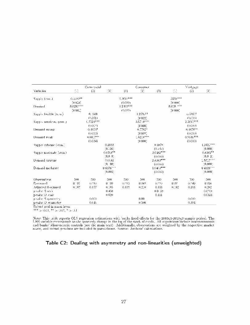
18See also the unweighted results in Table C2 in the Appendix.
16
credit is perceived as "moderately higher", and the value of -1 when lending conditions
are "moderately tighter" or when demand for credit is perceived as "moderately weaker".
The strong variable takes value of +1 when lending conditions are "extremely loosened" or
when demand for credit is perceived as "extremely higher", and the value of -1 when lend-
ing conditions "extremely tighter" or when demand for credit is perceived as "extremely
weaker". In all cases, these variables take the value of 0 otherwise.
Therefore, to deal with the issue of non-linearity we estimate an equation of the following
characteristics:
∆Yb,t = β0 + β1Xt + β2Xb,t−1 + (7)
β3cumLstrongbt + β4cumL
moderatebt + β5D
strongbt + β6D
moderatebt + fb + εb,t
The results are shown in column (3) of Table 6. For commercial loans, strong answers
in lending conditions and demand perceptions are not signi�cant. The e�ects on consumer
and mortgage loans are signi�cant at 10% and 1% respectively for supply conditions, and
at 1% respectively for demand perceptions. Despite that, the coe�cients associated to
stronger changes are, in general, bigger than the coe�cients associated to moderate changes.
Moreover, we test the hypothesis whether the coe�cients associated to strong changes are
equal to 1.5 the coe�cient associated to moderate changes for both, supply conditions and
demand perceptions.19 We found that the assumption of an strong answer has an impact
equal to 1.5 times the impact generated by a moderate answer is reasonable for commercial
and consumer credits, but not for mortgage loans, where the non-linearity appears to be
even stronger.
Taking all above analysis into account, the assumption of scaling the extreme values does
not have a signi�cant impact on the results, but the consideration of a possible asymmetry
improves the understanding of credit growth rates. In fact, our results in Table 6 show
that, by dealing with the asymmetric e�ects of supply conditions and demand perceptions,
the adjusted R-squared of our estimations can be improved signi�cantly in every market
segment. However, the impact on the adjusted goodness of �t is less signi�cant when
incorporating non-linearities.
19See "p-value S scale" and "p-vale D scale" at the bottom of Table 6.
17
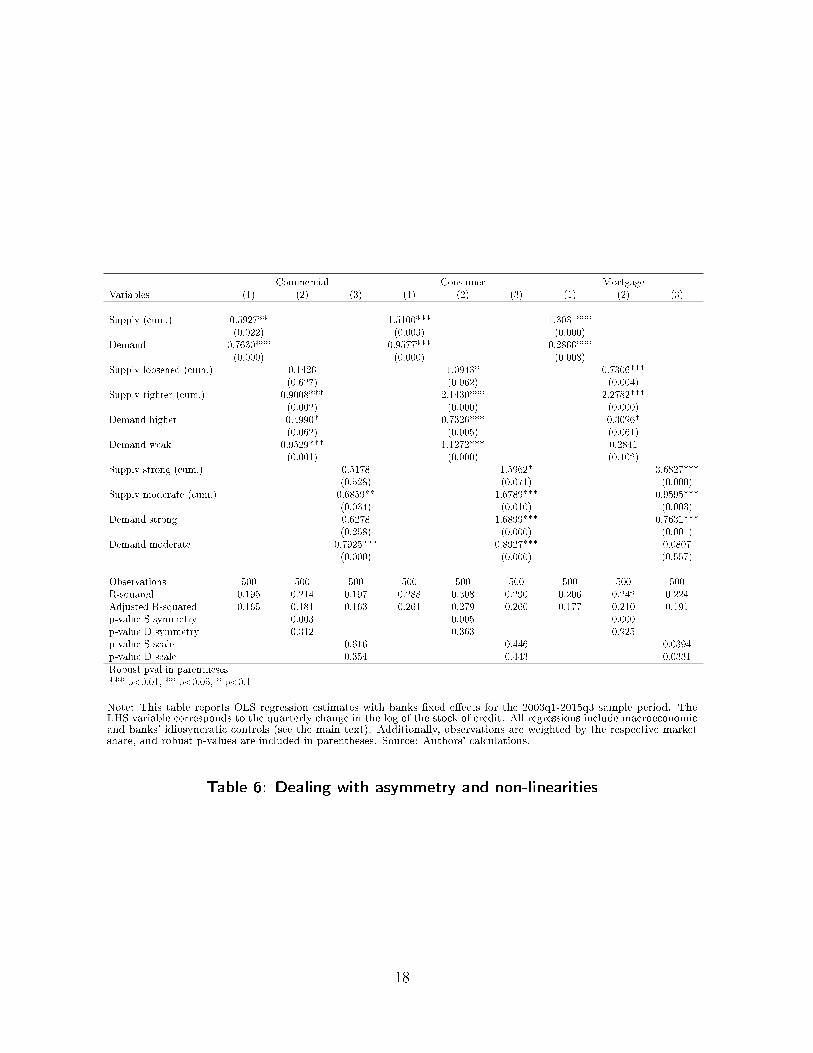
Commercial Consumer MortgageVariables (1) (2) (3) (1) (2) (3) (1) (2) (3)
Supply (cum.) 0.5927** 1.5100*** 1.3031***(0.022) (0.003) (0.000)
Demand 0.7630*** 0.9577*** 0.2866***(0.000) (0.000) (0.008)
Supply loosened (cum.) 0.1426 1.0943* 0.7306***(0.627) (0.062) (0.004)
Supply tighter (cum.) 0.9008*** 2.1430*** 2.2782***(0.002) (0.000) (0.000)
Demand higher 0.4990* 0.7326*** 0.3096*(0.062) (0.005) (0.061)
Demand weak 0.9529*** 1.1272*** 0.2841(0.001) (0.000) (0.102)
Supply strong (cum.) 0.5178 1.5962* 3.6827***(0.528) (0.071) (0.000)
Supply moderate (cum.) 0.6859** 1.6789*** 0.9595***(0.034) (0.010) (0.003)
Demand strong 0.6278 1.6899*** 0.7631***(0.258) (0.000) (0.001)
Demand moderate 0.7925*** 0.8927*** 0.0807(0.000) (0.000) (0.557)
Observations 500 500 500 500 500 500 500 500 500R-squared 0.195 0.214 0.197 0.288 0.308 0.290 0.206 0.242 0.224Adjusted R-squared 0.165 0.181 0.163 0.261 0.279 0.260 0.177 0.210 0.191p-value S symmetry 0.003 0.005 0.000p-value D symmetry 0.312 0.363 0.925p-value S scale 0.616 0.446 0.0394p-value D scale 0.354 0.443 0.0331Robust pval in parentheses*** p<0.01, ** p<0.05, * p<0.1
Note: This table reports OLS regression estimates with banks �xed e�ects for the 2003q1-2015q3 sample period. TheLHS variable corresponds to the quarterly change in the log of the stock of credit. All regressions include macroeconomicand banks' idiosyncratic controls (see the main text). Additionally, observations are weighted by the respective marketshare, and robust p-values are included in parentheses. Source: Authors' calculations.
Table 6: Dealing with asymmetry and non-linearities
18
5 Conclusions
Among central banks, senior loan o�cers' surveys are widely used to comprehend the role
of banks in the credit channel and their in�uence in the transmission of monetary policy,
beyond the interest rate e�ects on credit demand. After the global �nancial crisis, this
information has been used to conduct various studies that show the relevance of these
instruments in explaining the dynamics of credit, especially during turbulent economic
times.
The Chilean SLOS version named "Encuesta de Crédito Bancario" (ECB) is applied
in a quarterly frequency since 2003. In this paper we use the information embedded in
the Chilean SLOS and complement it by building a complete panel dataset at the bank
level that includes banks' idiosyncratic characteristics and macroeconomic factors. In a
similar way to Calani et al. (2010) we investigate the role of the ECB in explaining credit
growth. However, we extend the analysis in various respects. First, we re�ne the variables'
frequency and de�nitions, in order to improve the estimations' statistical properties and
save degrees of freedom. Additionally, we investigate the potential asymmetric in�uence of
perception in the credit dynamics. Finally, we are able to compare the magnitude of the
in�uence of credit standards and demand perceptions.
We �nd that the in�uence of credit standards and demand perceptions is statistically
and economically relevant to determine credit growth. Various pieces of evidence point
out in that direction, namely the regression coe�cients, standard errors, and the survey
variables' contribution in explaining total credit growth variance. This result holds for all
market segments and is robust to various idiosyncratic and standard macro variables as
controls. Additionally, the evidence suggests that the perceptions' impact is asymmetric,
being more relevant during contractionary credit conditions. Thus, our results provide
evidence to the issue that �nancial cycles tend to be more persistent than economic cy-
cles (Borio, 2014), provided that bankers tighten their lending conditions before economic
downturns, and loosen them afterwards.
Motivated by the results of the present investigation, we propose to continue this line
of research by creating more accurate indices of credit activity that help in macroeconomic
forecasting models. However, we leave these developments for future works.
19
References
[1] Avanzini D. and A. Jara (2015). The use of data reduction techniques to assess systemic
risk: An application to the Chilean banking system. Intelligent Data Analysis, 19(s1),
S45-S67.
[2] Balasubramanyan L., Z. Saeed, and J. Thomson (2014). Are banks forward-looking
in their loan loss provisioning? Evidence from the senior loan o�cer opinion survey
(SLOOS). Working Paper No. 13-13R , Federal Reserve Bank of Cleveland.
[3] Bassett W. F., M. B. Chosak, J. C. Driscoll, and E. Zakrajsek. (2014). Changes in
bank lending standards and the macroeconomy. Journal of Monetary Economics, 62,
23-40.
[4] Bell V. and A. Pugh (2014). The Bank of England credit conditions survey. Working
Paper No. 515, Bank of England.
[5] Berg J., A. Van Rixtel, A. Ferrando, G. De Bondt, and S. Scopel (2005). The bank
lending survey for the euro area. Occasional paper, No. 23, European Central Bank.
[6] Bernanke B. and M. Gertler (1995). Inside the black box: the credit channel of mon-
etary policy transmission. Working Paper No. 5146, National Bureau of Economic
Research.
[7] Blaes, B. (2011). Bank-related loan supply factors during the crisis: An analysis based
on the German bank lending survey. Discussion Paper Series 1 (No. 2011, 31), Deutsche
Bundesbank.
[8] Breeden, J. and J. Canals-Cerdá (2016). Consumer risk appetite, the credit cycle, and
the housing bubble. Working paper No. 16-05, Federal Researve Bank of Philadelphia.
[9] Borio, C. (2014). The �nancial cycle and macroeconomics: What have we learnt?
Journal of Banking & Finance, 45 182-198.
[10] Calani, M., P. García, and D. Oda. (2010). Supply and demand identi�cation in the
credit market. Working Paper No. 571, Central Bank of Chile.
20
[11] Ciccarelli M., A. Maddaloni, and J. L. Peydró (2010). Trusting the bankers: A new
look at the credit channel of monetary policy. Working paper No. 1228, European
Central Bank.
[12] Cunningham (2006). The predictive power of the senior loan o�cer survey: do lending
o�cers know anything special? Federal Reserve Bank of Atlanta, Working Paper
2006-24.
[13] De Bondt G., A. Maddaloni, J. L. Peydró, and S. Scopel. (2010). The Euro area bank
lending survey matters: Empirical evidence for credit and output growth. Working
Paper No 1160, European Central Bank.
[14] Del Giovane P., G. Eramo, and A. Nobili (2011). Disentangling demand and supply in
credit developments: A survey-based analysis for Italy. Journal of Banking & Finance
35(10):2719(2732).
[15] Jara, A. and C. G. Silva. (2007). Metodología de la encuesta sobre condiciones generales
y estándares en el mercado de crédito bancario. Economic and Statisical Studies Series,
No. 57, Central Bank of Chile.
[16] Keeton W. (1999). Does faster loan growth lead to higher loan losses? Economic
Review 84(2) 57, Federal Reserve Bank Of Kansas City.
[17] Lown, C. S., D. P. Morgan, and S. Rohatgi. (2000). Listening to loan o�cers: The im-
pact of commercial credit standards on lending and output. Economic Policy Review,
6(2), Federeal Researve Bank of New York.
[18] Lown, C., and D. P. Morgan. (2006). The credit cycle and the business cycle: New
�ndings using the loan o�cer opinion survey. Journal of Money, Credit and Banking,
1575-1597.
[19] Milani, F. (2007). Expectations, learning and macroeconomic persistence. Journal of
Monetary Economics, 54(7) 2065-2082.
[20] Waters G. (2012). Quantity rationing of credit. Research Discussion Paper No. 3, Bank
of Finland.
21
Appendix A. Conceptual framework
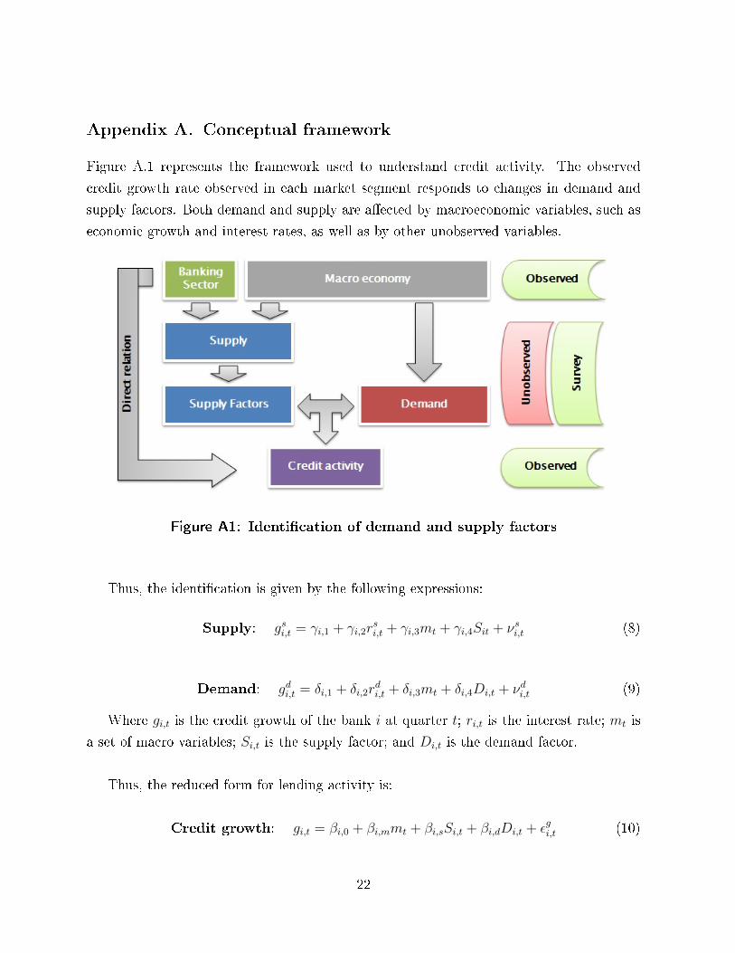
Figure A.1 represents the framework used to understand credit activity. The observed
credit growth rate observed in each market segment responds to changes in demand and
supply factors. Both demand and supply are a�ected by macroeconomic variables, such as
economic growth and interest rates, as well as by other unobserved variables.
Figure A1: Identi�cation of demand and supply factors
Thus, the identi�cation is given by the following expressions:
Supply: gsi,t = γi,1 + γi,2rsi,t + γi,3mt + γi,4Sit + νsi,t (8)
Demand: gdi,t = δi,1 + δi,2rdi,t + δi,3mt + δi,4Di,t + νdi,t (9)
Where gi,t is the credit growth of the bank i at quarter t; ri,t is the interest rate; mt is
a set of macro variables; Si,t is the supply factor; and Di,t is the demand factor.
Thus, the reduced form for lending activity is:
Credit growth: gi,t = βi,0 + βi,mmt + βi,sSi,t + βi,dDi,t + εgi,t (10)
22
which must meet the following conditions:
Credit growth: βi,s =γi,4δi,2δi,2 − γi,2
> 0 ∧ βi,d = − γi,2δi,4δi,2 − γi,2
> 0
Note that when we aggregate the data at system level we introduce a bias equivalent
to:
gi,t ≡li,t − li,t−1li,t−1
(11)
with the following dynamics:
git = βi,0 + βmmt + βzzi,t + βssi,t + βddi,t + ξi,t (12)
Then, the aggregate growth dynamics corresponds to:
Gt ≡∑N
i=1 (li,t − li,t−1)∑Ni=1 li,t−1
= A+ βmmt + βzZt + βsSt + βdDt + Et + Γt (13)
where ωt−1 is the vector of market shares at quarter t− 1; Et = ω′t−1ξi,t; and
Γt =(ω′t−1β0 − A
)+ βz
(Zt − ω′t−1zt
)
23
Appendix B. Additional �gures
Note: These �gures compare the standard deviation of the answers reported by the SLOS and the respectiveaggregate supply condition and demand perception. Source: Authors' calculations based on the Senior LoanO�cers Survey, Central Bank of Chile.
Figure B1: Dispersion of lending standards and demand perceptions:
corporate loans
24
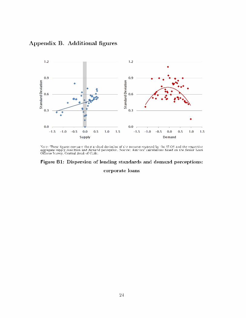
Note: This �gure shows the annual growth rate for corporate loans and the factors (controls, supply,demand, error) that explain that change according to the regression estimated in column (3) of Table 2 forconsumer loans. Source: Authors' calculations based on the Senior Loan O�cers Survey, Central Bank of Chile.
Figure B2: Sources of lending growth rates for consumer loans
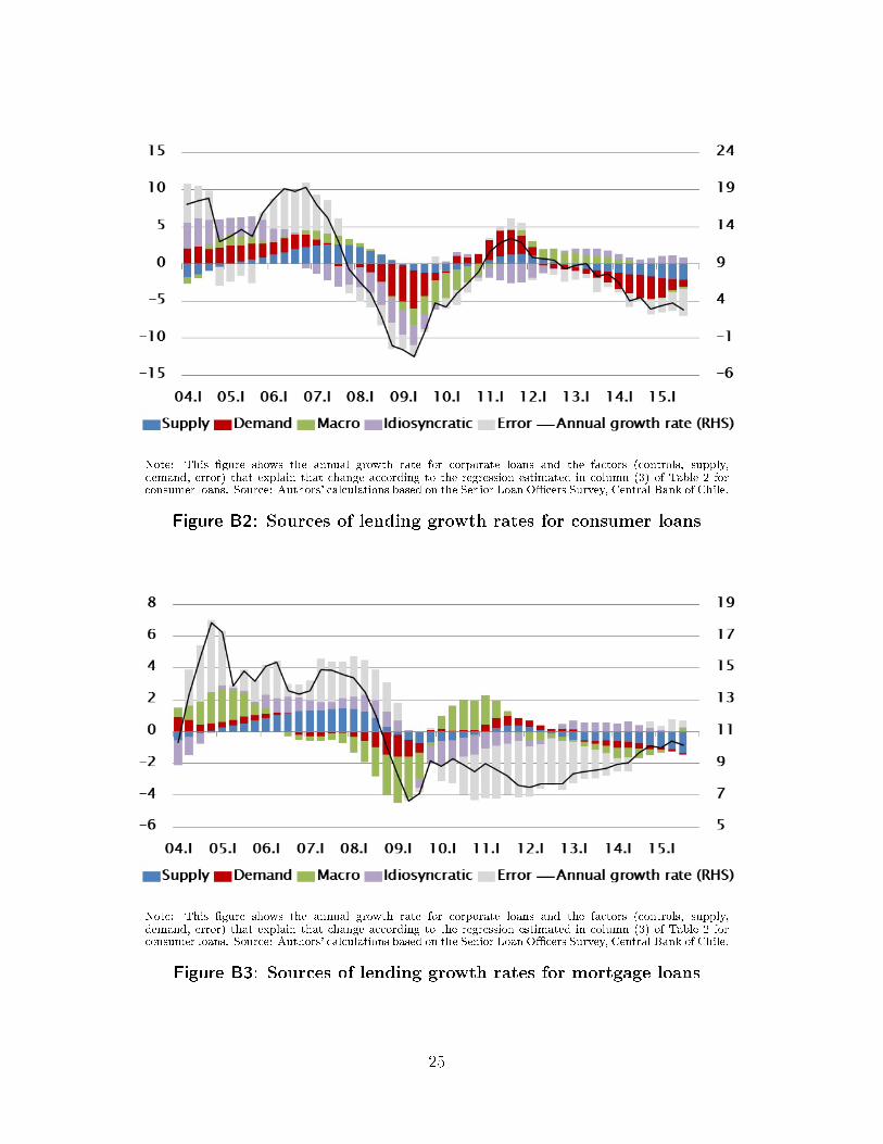
Note: This �gure shows the annual growth rate for corporate loans and the factors (controls, supply,demand, error) that explain that change according to the regression estimated in column (3) of Table 2 forconsumer loans. Source: Authors' calculations based on the Senior Loan O�cers Survey, Central Bank of Chile.
Figure B3: Sources of lending growth rates for mortgage loans
25
Appendix C. Additional tables
Commercial Consumer MortgageVariables (1) (2) (3) (1) (2) (3) (1) (2) (3)
Supply 0.1304 0.4071** 0.0125(0.426) (0.014) (0.928)
Demand 0.6419*** 0.6297*** 1.1687*** 1.2493*** 0.7126*** 0.6701***(0.000) (0.001) (0.000) (0.000) (0.000) (0.000)
Supply (cum.) 0.6887*** 0.5580** 2.6606*** 2.4618*** 1.5002*** 1.2234***(0.005) (0.019) (0.000) (0.000) (0.000) (0.000)
Demand (cum.) -0.0438 -0.6771 -0.2287(0.832) (0.160) (0.351)
Observations 500 500 500 500 500 500 500 500 500R-squared 0.191 0.172 0.197 0.193 0.181 0.213 0.201 0.190 0.221Adjusted R-squared 0.161 0.141 0.167 0.162 0.150 0.183 0.171 0.159 0.192
Robust pval in parentheses*** p<0.01, ** p<0.05, * p<0.1
Note: This table reports OLS regression estimations with banks �xed e�ects for the 2003q1-2015q3 sample period. TheLHS variable corresponds to the quarterly change in the log of the stock of credit. All regressions include macroeconomicand banks' idiosyncratic controls (see the main text). Robust p-values are included in parentheses. Source: Authors'calculations.
Table C1: The role of SLOS on banks' lending growth rates(unweighted)
26
Commercial Consumer MortgageVariables (1) (2) (3) (1) (2) (3) (1) (2) (3)
Supply (cum.) 0.5580** 2.4618*** 1.2234***(0.019) (0.000) (0.000)
Demand 0.6297*** 1.2493*** 0.6701***(0.001) (0.000) (0.000)
Supply �exible (cum.) 0.1569 1.2730** 0.5865*(0.571) (0.022) (0.056)
Supply restricted (cum.) 0.7524*** 3.5710*** 2.5615***(0.002) (0.000) (0.000)
Demand strong 0.4854* 0.7762* 0.4876**(0.053) (0.092) (0.050)
Demand weak 0.6917** 1.6218*** 0.9146***(0.034) (0.000) (0.000)
Supply extreme (cum.) 0.2833 0.4078 4.1621***(0.726) (0.747) (0.000)
Supply moderate (cum.) 0.6768** 3.0482*** 0.8381**(0.018) (0.000) (0.012)
Demand extreme 0.6682 2.8383*** 1.5717***(0.198) (0.000) (0.000)
Demand moderate 0.6376*** 1.0403*** 0.4328***(0.002) (0.000) (0.009)
Observations 500 500 500 500 500 500 500 500 500R-squared 0.197 0.210 0.199 0.213 0.242 0.220 0.221 0.249 0.234Adjusted R-squared 0.167 0.177 0.165 0.183 0.210 0.188 0.192 0.218 0.202p-value S scale 0.450 0.0159 0.0201p-value D scale 0.620 0.111 0.0421p-value S symmetry 0.009 0.001 0.000p-value D symmetry 0.646 0.306 0.304Robust pval in parentheses*** p<0.01, ** p<0.05, * p<0.1
Note: This table reports OLS regression estimations with banks �xed e�ects for the 2003q1-2015q3 sample period. TheLHS variable corresponds to the quarterly change in the log of the stock of credit. All regressions include macroeconomicand banks' idiosyncratic controls (see the main text). Additionally, observations are weighted by the respective marketshare, and robust p-values are included in parentheses. Source: Authors' calculations.
Table C2: Dealing with asymmetry and non-linearities (unweighted)
27
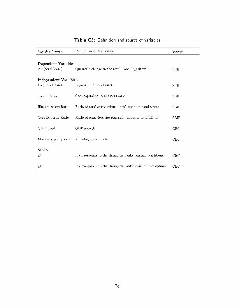
Table C3: De�nition and source of variables
Variable Names Report Form Description Source
Dependent Variables
∆ln(total loans) Quarterly change in the total loans' logarithm. SBIF
Independent Variables.
Log Total Assets Logarithm of total assets SBIF
Tier 1 Ratio Core capital to total assets ratio. SBIF
Illiquid Assets Ratio Ratio of total assets minus liquid assets to total assets SBIF
Core Deposits Ratio Ratio of term deposits plus sight deposits to liabilities. SBIF
GDP growth GDP growth. CBC
Monetary policy rate Monetary policy rate. CBC
SLOS
Lc It corresponds to the change in banks' lending conditions. CBC
Dp It corresponds to the change in banks' demand perceptions CBC
28
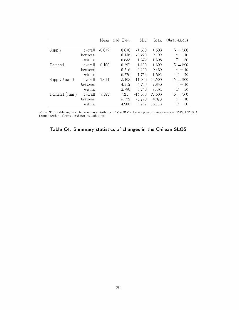
Mean Std. Dev. Min Max Observations
Supply overall -0.012 0.646 -1.500 1.500 N = 500between 0.136 -0.220 0.190 n = 10within 0.633 -1.572 1.598 T = 50
Demand overall 0.166 0.797 -1.500 1.500 N = 500between 0.216 -0.290 0.460 n = 10within 0.770 -1.754 1.596 T = 50
Supply (sum.) overall 1.614 5.108 -11.000 13.500 N = 500between 4.512 -5.700 7.850 n = 10within 2.780 -6.236 8.494 T = 50
Demand (cum.) overall 7.583 7.217 -14.500 25.500 N = 500between 5.579 -3.720 14.370 n = 10within 4.900 -5.787 18.713 T = 50
Note: This table reports the summary statistics of the SLOS for corporate loans over the 2003q1-2015q3sample period. Source: Authors' calculations.
Table C4: Summary statistics of changes in the Chilean SLOS
29
Documentos de Trabajo
Banco Central de Chile
NÚMEROS ANTERIORES
La serie de Documentos de Trabajo en versión PDF
puede obtenerse gratis en la dirección electrónica:
www.bcentral.cl/esp/estpub/estudios/dtbc.
Existe la posibilidad de solicitar una copia impresa
con un costo de Ch$500 si es dentro de Chile y
US$12 si es fuera de Chile. Las solicitudes se pueden
hacer por fax: +56 2 26702231 o a través del correo
electrónico: [email protected].
Working Papers
Central Bank of Chile
PAST ISSUES
Working Papers in PDF format can be
downloaded free of charge from:
www.bcentral.cl/eng/stdpub/studies/workingpaper.
Printed versions can be ordered individually for
US$12 per copy (for order inside Chile the charge
is Ch$500.) Orders can be placed by fax: +56 2
26702231 or by email: [email protected].
DTBC – 801
Pruebas de Tensión Bancaria del Banco Central de Chile: Actualización
Juan-Francisco Martínez, Rodrigo Cifuentes y J. Sebastián Becerra
DTBC – 800
Unemployment Dynamics in Chile: 1960-2015
Alberto Naudon y Andrés Pérez
DTBC – 799
Forecasting Demand for Denominations of Chilean Coins and Banknotes
Camila Figueroa y Michael Pedersen
DTBC – 798
The Impact of Financial Stability Report’s Warnings on the Loan to Value Ratio
Andrés Alegría, Rodrigo Alfaro y Felipe Córdova
DTBC – 797
Are Low Interest Rates Deflationary? A Paradox of Perfect-Foresight Analysis
Mariana García-Schmidt y Michael Woodford
DTBC – 796
Zero Lower Bound Risk and Long-Term Inflation in a Time Varying Economy
Benjamín García
DTBC – 795
An Analysis of the Impact of External Financial Risks on the Sovereign Risk Premium
of Latin American Economies
Rodrigo Alfaro, Carlos Medel y Carola Moreno
DTBC – 794
Welfare Costs of Inflation and Imperfect Competition in a Monetary Search Model
Benjamín García
DTBC – 793
Measuring the Covariance Risk Consumer Debt Portfolios
Carlos Madeira
DTBC – 792
Reemplazo en Huelga en Países Miembros de la OCDE: Una Revisión de la
Legislación Vigente
Elías Albagli, Claudia de la Huerta y Matías Tapia
DTBC – 791
Forecasting Chilean Inflation with the Hybrid New Keynesian Phillips Curve:
Globalisation, Combination, and Accuracy
Carlos Medel
DTBC – 790
International Banking and Cross-Border Effects of Regulation: Lessons from Chile
Luis Cabezas y Alejandro Jara
DTBC – 789
Sovereign Bond Spreads and Extra-Financial Performance: An Empirical Analysis of
Emerging Markets
Florian Berg, Paula Margaretic y Sébastien Pouget
DTBC – 788
Estimating Country Heterogeneity in Capital-Labor substitution Using Panel Data
Lucciano Villacorta
DTBC – 787
Transiciones Laborales y la Tasa de Desempleo en Chile
Mario Marcel y Alberto Naudon

DOCUMENTOS DE TRABAJO • Junio 2017