Embed Size (px)
Citation preview

Basic templateSubtitle
Location – Datewww.ing.com
Name of the speakerJob title

ING 2
Executive Champion: <NAME>Local Champion: <NAME>Process Owner(s): <NAME(s)>Master Black Belt: <NAME>Black Belt: <NAME>Green Belt: <NAME>Financial Analyst: <NAME>
Other Team Members: <NAMES>
Related Projects: <If Applicable>
Project Name
ICE Country and Functional LineAdvisors NetworkFinanceHuman ResourcesLegal / ComplianceCustomer ServiceDefined ContributionEmployee BenefitsInformation TechnologyMarketingMutual FundsRetail AnnuityRetail LifeReinsurance / Institutional Markets
Tollgate Stage MM /DD/ YYYY
Project ID:

ING 3
DMAIC Process Steps
Define Measure Analyze Improve Control
Project CCR’sValidated VOCCompleted Team CharterPreliminary CBA EstimateValidated Process Map Identify Quick Wins Identify Issues & BarriersProject Schedule
List of Potential Root CausesList of Statistically Significant XsDemonstrate Relationship of X’s to YPreliminary CBA Process Evaluation
Develop to be processDemonstrateImprovements via PilotGraphical Analysis of Pilot Finance Approved CBA
MSA Results on XsNew Process PerformanceStatistical Confirmation ofImprovementsProcess ManagementSystem Plan (SPC)Process Owner HandoffFinal CBA
Completed QFD/CCR TreeOperational DefinitionsSpecification LimitsStated TargetsDefect DefinitionsMeasurement PlanMeasurement SystemAnalysisGraphical AnalysisRolled Through Put YieldBaseline Current ProcessPerformance ( Z st)
Key Deliverables:
•Surveys•Focus Groups•Interviews•SIPOC•Functional Deployment •Map•FAST, Stakeholder Analysis
•QFD / CCR Tree•Measurement Plan•Continuous Gage R&R•Attribute Gage R&R•Sample Size Calculator•Pareto Charts•Graphical Summary•Line Charts•Benchmarking•Process Capability
•Dot Plots•Box Plots•Run Charts•Normality Testing•Fishbone Diagram•Hypothesis Testing•Regression Analysis•DOE•NVA and VA Analysis
•Pugh Matrix•New Functional Deployment •Map•FMEA on new process•Pilot
•Continuous Gage R&R•Attribute Gage R&R•Control Charts•Hypothesis Testing•Control Plan•Process Capability
1)
2)
3)
Tools
1. Identify Critical Customer Requirements
2. Develop Team Charter
3. Develop Process Maps
4. Select Critical Customer Requirement
5. Data Collection Plan Validate MSA on (Y’s)
6. Calculate Baseline Process Capability
7. Identify Potential Root Causes
8. Validate Root Causes
9. Evaluate Root Cause Relationships ( y = f (x))
10.Develop Improvements
11.Confirm Results and Validate Improvements
12.Validate MSA on X’s
13.Calculate New Process Capability
14. Implement Process Control

ING 4
Project CCR’sValidated VOCCompleted Team CharterPreliminary CBA EstimateValidated Process Map Identify Quick Wins Identify Issues & BarriersProject Schedule
List of Potential Root CausesList of Statistically Significant XsDemonstrate Relationship of X’s to YPreliminary CBA Process Evaluation
Develop to be processDemonstrateImprovements via PilotGraphical Analysis of Pilot Finance Approved CBA
MSA Results on XsNew Process PerformanceStatistical Confirmation ofImprovementsProcess ManagementSystem Plan (SPC)Process Owner HandoffFinal CBA
Completed QFD/CCR TreeOperational DefinitionsSpecification LimitsStated TargetsDefect DefinitionsMeasurement PlanMeasurement SystemAnalysisGraphical AnalysisRolled Through Put YieldBaseline Current ProcessPerformance ( Z st)
Key Deliverables:
•Surveys•Focus Groups•Interviews•SIPOC•Functional Deployment •Map•FAST, Stakeholder Analysis
•QFD / CCR Tree•Measurement Plan•Continuous Gage R&R•Attribute Gage R&R•Sample Size Calculator•Pareto Charts•Graphical Summary•Line Charts•Benchmarking•Process Capability
•Dot Plots•Box Plots•Run Charts•Normality Testing•Fishbone Diagram•Hypothesis Testing•Regression Analysis•DOE•NVA and VA Analysis
•Pugh Matrix•New Functional Deployment •Map•FMEA on new process•Pilot
•Continuous Gage R&R•Attribute Gage R&R•Control Charts•Hypothesis Testing•Control Plan•Process Capability
1)
2)
3)
Define Measure Analyze Improve Control
Tools
1.Identify Critical Customer Requirements
2.Develop Team Charter
3.Develop Process Maps
4. Select Critical Customer Requirement
5. Data Collection Plan Validate MSA on (Y’s)
6. Calculate Baseline Process Capability
7.Identify Potential Root Causes
8.Validate Root Causes
9.Evaluate Root Cause Relationships ( y = f (x))
10.Develop Improvements
11.Confirm Results and Validate Improvements
12.Validate MSA on X’s
13.Calculate New Process Capability
14. Implement Process Control
DMAIC Process Steps

ING 5
Identify Potential Root CausesAnalyze - Step 7
Potential Root causes of your Defect:• Use a Pareto to Stratify and Identify root causes• Single Case Boring Tool
Pareto Charts
Co
un
t
Pe
rce
nt
Plan NameCount
18.9 6.8 4.5Cum % 43.3 69.9 88.8 95.5 100.0
16104 9900 7030 2520 1665Percent 43.3 26.6
OtherABCZZTopMMMXYZ
40000
30000
20000
10000
0
100
80
60
40
20
0
Pareto Chart of Plan Name
Co
un
t
Pe
rce
nt
Plan NameCount
18.9 6.8 4.5Cum % 43.3 69.9 88.8 95.5 100.0
16104 9900 7030 2520 1665Percent 43.3 26.6
OtherABCZZTopMMMXYZ
40000
30000
20000
10000
0
100
80
60
40
20
0
Pareto Chart of Plan NameC
ou
nt
Pe
rce
nt
Plan NameCount
18.9 6.8 4.5Cum % 43.3 69.9 88.8 95.5 100.0
16104 9900 7030 2520 1665Percent 43.3 26.6
OtherABCZZTopMMMXYZ
40000
30000
20000
10000
0
100
80
60
40
20
0
Pareto Chart of Plan Name

ING 6
Identify Potential Root Causes
What are the Potential
Causes of the Defect?
(Enter in the form of a question)
Effect (Y)Potential Causes (Xs)
Forms Staff / People
Methods / Procedures Systems / Equipment
Measurement
Environment
Teams working on the same process
at different sites
Multiple systems
Poor data entry
Faulty data reporting
Application form not correct
Staff not trained
Analyze - Step 7

ING 7
Analyze - Step 8
Stability Shape Spread
(Variance)
Centering
Use Control or Run Charts, Box Plots and Dot plots to detect significant runs, trends or patterns in the data
Use Histograms,
Normality Plots and the Graphical Summary from Minitab to determine normality
P<0.05 data is
NOT normal
Use the Homogeneity of variance test to determine if the variances of the two populations are equal.
P<0.05 variances
NOT Equal
Use ANOVA or Mood’s median testing to determine if the centers of the two populations are equal.
P<0.05 Centering
NOT Equal
Hypothesis Testing
Validate Root Causes
Statistical Testing Overview

ING 8
Statistical Testing - StabilityAnalyze - Step 8
Observation
Ind
ivid
ua
l V
alu
e
181161141121101816141211
10.0
7.5
5.0
2.5
0.0
_X=4.56
UCL=9.16
LCL=-0.04
Observation
Mo
vin
g R
an
ge
181161141121101816141211
8
6
4
2
0
__MR=1.730
UCL=5.652
LCL=0
7
7
77
7
77
7
777
7
7
1
1
8
6
5
8
66
11
1
5
22222
22222
2
2
2222
22
11111
1
1
44
4
1
1
I -MR Chart of Cycle Time
Observation
Cycl
e T
ime
200180160140120100806040201
10
8
6
4
2
0
Number of runs about median:
0.44363
102Expected number of runs: 101.00000Longest run about median: 8Approx P-Value for Clustering: 0.55637Approx P-Value for Mixtures:
Number of runs up or down:
0.36808
135Expected number of runs: 133.00000Longest run up or down: 5Approx P-Value for Trends: 0.63192Approx P-Value for Oscillation:
Run Chart of Cycle Time
Stacked
Loca
tion
11.29.68.06.44.83.21.60.0
Denver
Minot
Dotplot of Stacked vs Location
Data
DenverMinot
12
10
8
6
4
2
0
Boxplot of Minot, Denver
Run Chart Box Plot
I-MR Chart DOT Plot

ING 9
Statistical Testing – Road MapSTART:
Is Y Continuousor Discrete?
Is X Continuousor Discrete?
Variation or
Centering?
Chi Square
Binomial
Regression
Scatter Plot
Discrete (Y)
Discrete (X)
Continuous (X)
Continuous (Y)
Variation Centering
Variance Test Bartlett
Variance Test
F-Test
Is X Continuousor Discrete?
Normal ornon-Normal?
Normal ornon-Normal?
Variance Test Levine
Normal Non-Normal
Comparing Relative to a
Target?
Comparing Only Two Samples?
Normal Non-Normal
ANOVA
One Sample T-Test
Two Sample T-Test
No No
LogisticRegression
Non-Parametri
c Tests
Mann-Whitney
Mood’s Median
Yes Yes
Continuous (X)Discrete (X)

ING 10
Regression Process flow
Important X
Calculate relative regression
Rsqr highNot an important X
Normally distributedP>0,05NO regression possible
Regression possible
Y
N
N
Check residuals with Minitab with 4 in 1 table option (check 3 tables)
Megaphone shape
NO regression possible
NO regression possible
trends, outliers,non-random patterns
Y
Y
N
N
Y

ING 11
Statistical Analysis: Regression
• What: Regression
• When:• In order to define a mathematical
relationship (model) between two continuous variables
• Continuous Y, continuous X
• Where:• Stat > Regression > Fitted Line
Plot
• Assumptions:• Assumptions are made particulary
about error or “residuals” (explanation later).
• Why:• Relationship between the two
variables
• Predictive formula (you could estimate future cycle times based on the approval times) y=b+mx
• Percent of the variation in the response variable that can be attributed to the predictor variable

ING 12
Exercise: Regression
1510 5 0
30
20
10
0
Approval Time (Days)
Cyc
le T
ime
S = 0.981474 R-Sq = 95.7 % R-Sq(adj) = 95.7 %
Cycle Time = -0.564507 + 1.99361 Approval Tim
Regression Plot: Cycle Time vs. Approval Time

ING 13
Strong R2Strong R2
Review results and check for outliers
The regression equation isY3 = 3.02 + 0.505 X3
Predictor Coef StDev T PConstant 3.015 1.080 2.79 0.021X3 0.5051 0.1178 4.29 0.002
S = 1.173 R-Sq = 67.1% R-Sq(adj) = 63.5%
Analysis of Variance
Source DF SS MS F PRegression 1 25.283 25.283 18.37 0.002Residual Error 9 12.387 1.376Total 10 37.669
Unusual ObservationsObs X3 Y3 Fit StDev Fit Residual St Resid 10 13.0 12.500 9.581 0.621 2.919 2.93R
R denotes an observation with a large standardized residual
Low p ValueLow p Value
Row 10Outlier
Row 10Outlier

ING 14
Mean:0.0143624
StDev:1.05039
ML Estimates
-3 -2 -1 0 1 2 3
1
5
10
20
3040506070
80
90
95
99
Data
Pe
rce
nt
Normal Probability Plot for SRES1
Residual Plot 1: The residuals should be normally distributed for a good regression
A probability plot of the previous data (Y3, X3) shows oneoutlier is different from the rest of the data
A probability plot of the previous data (Y3, X3) shows oneoutlier is different from the rest of the data

ING 15
Residuals Plot 2:Residuals Against the Fitted Values
Why?
• To look for a non-random pattern, such as a megaphone (funnel) shape.
• The megaphone shape indicates that variation increases as the response increases. Conclusions can be affected and may be incorrect.
• Ignore the pattern indicated by the symmetry of the dots around 0. It is not a special cause. Two replicates will always appear perfectly matched.
30 40 50 60-2.5-2.0-1.5-1.0-0.50.00.51.01.52.02.5
Fitted Value
Sta
ndar
dize
d R
esid
ual
Residuals Versus the Fitted Values(response is No. of Bends)
30 40 50 60-2.5-2.0-1.5-1.0-0.50.00.51.01.52.02.5
Fitted Value
Sta
ndar
dize
d R
esid
ual
Residuals Versus the Fitted Values(response is No. of Bends)

ING 16
Residuals Plot 3:Residuals Against Time Order
Why?
• To ensure that the experimental variability has only common causes associated with it. The relationship should not change over time.
• To look for lurking variables (trends, outliers, or non-random patterns) that might influence our conclusions. They may have been hidden in other plots.
2 4 6 8 10 12 14 16-2.5
-2.0-1.5
-1.0
-0.5
0.00.5
1.0
1.52.0
2.5
Observation Order
Sta
nd
ard
ize
d R
esi
du
al
Residuals Versus the Order of the Data(response is No. of Bends)
2 4 6 8 10 12 14 16-2.5
-2.0-1.5
-1.0
-0.5
0.00.5
1.0
1.52.0
2.5
Observation Order
Sta
nd
ard
ize
d R
esi
du
al
Residuals Versus the Order of the Data(response is No. of Bends)

ING 17
Statistical Analysis: Multiple Regression
• What: Multiple Regression
• When:• Upon determine there is a
relationship between a response variable and multiple predictor variables
• Continuous Y, continuous X’s
• Where:• Stat > Regression > Regression
• Why:• Same predictive formula as with
Regression
• Quantify relationship between multiple predictors and single response variable

ING 18
• Start off by creating a matrix plot which shows the relationship between each X and the Y as well as between each pair of Xs:
• Mail Sort Time, Approval Time and Waiting for Info seem to influence y.
Cycle Time
Approval Time
Waiting for Info
No. of Staff
Mail Sort Time
604020 15010050 7,04,52,0 605040
40
20
060
40
20
150
100
50
7,0
4,5
2,0
Matrix Plot
Multiple Regression – Example

ING 19
Statistical Analysis: Logistic Regression
• What: Logistic Regression• Since Y in not continuous, the
probability of an event (discrete Y) is modeled using the “logit” function from which this regression tool gets its name
• When:• In order to test for statistically
significant differences between groups
• Discrete Y, continuous X
• Where:• Stat > Regression > Binary Logistic
Regression
• Why:• To investigate the relationship
between a categorical response variable and one or more predictors

ING 20
Hypothesis Testing: 2-sample t-Test
• What: t-Test
• When to use:• To determine if there is a
significant difference between the averages of two groups
• Continuous Y, discrete X
• Where:• Stat > Basic Statistics > 2-sample t
• Assumptions:• The data within each group are
normally distributed.
• Why: • To determine if the two groups of
a discrete x-variable are significantly different, indicating that this x has an influence on the y.

ING 21
Anova Process flow
Test normality within groups
P>0,05Transform data
Test for equal variability
P>0,05
ANOVA test
P<0,05
Different 2 sample t-Test
No important X
Important X
Look at Bartlett, since data is normally distributed
Y
Y
Y
N
N
N

ING 22
Statistical Analysis: ANOVA (One-way)
• What: ANOVA (One-way)
• When:• Testing to determine if 3 or more
groups are statistically different
• Continuous Y, discrete X
• Where:• Stat > ANOVA > One-way
• Assumptions:• The data within each group are
normally distributed
• The groups have equal variances
• Why:• To determine if there is a
significant (statistical) difference between 3 or more groups
Validate Root Causes

ING 23
New
Yor
k
Par
is
Syd
ney
1
2
3
4
5
Location
Cus
t. S
at
Boxplots of Customer Satisfaction by Location(means are indicated by solid circles)
Exercise: ANOVA (One-way)
Analysis of Variance for Cust. SaSource DF SS MS F PLocation 2 475.967 237.984 265.16 0.000Error 2017 1810.276 0.898Total 2019 2286.243 Individual 95% CIs For Mean Based on Pooled StDevLevel N Mean StDev ----------+---------+---------+------New York 1021 4.0627 0.9096 (*) Paris 503 4.4632 0.6360 (*-) Sydney 496 3.1331 1.2417 (-*) ----------+---------+---------+------Pooled StDev = 0.9474 3.50 4.00 4.50
Validate Root Causes

ING 24
Statistical Analysis: Contingency Tables
• What: Contingency Tables
• When:• In order to test for statistically
significant differences between two or more groups
• Discrete Y, discrete X
• Where:• Stat > Tables > Cross Tabulation
• Why:• Tests for significance between two
or more discrete groups
Validate Root Causes

ING 25
Hypothesis Testing: Chi-Square Test
What: Chi-Square Test
When:– Testing to determine if two or
more groups are statistically different in their averages
– Discrete Y, discrete X
Where:– Stat > Tables > Chi-Square
Test
Assumptions:– You have enough data
(counts) so that the expected counts for each cell are >5
Why: – To verify if the two or more
groups of a discrete x-variable are significantly different, indicating that this x has an influence on the discrete y.

ING 26
Chi-Square in Minitab
• Open the exercise file „Product Satisfaction“
• Go to „Stat“ and „Tables“
• The sample data worksheet contains both the raw and the table data.
•In general, if you only have raw data, then use the „Cross Tabulation and Chi-Square“ function in Minitab. This will calculate the counts you need to create a tableof your raw data manually. You can also have Minitab do the Chi-Square test right away by clicking on the button „Chi-Square“. Indicate that you also want to see theexpected counts.
• When your data is in table form, you can also use the function „Chi-SquareTest (Table in Worksheet)“ to get the same results. In this case you simply selectall the columns that make up the table (here: four columns).

ING 27
How the Chi-Square Test Works
The Chi-square Test calculates “expected counts” (e.g. 857.63) for each cell, based on the relationships of the totals. The test then compares these expected count with the actual counts of each cell (e.g. 850) and determines if there is a significant difference between the expected and actual. If there is a significant difference somewhere, then the p-value will be low. Here, y = satisfaction, x = customer category Men
Over 40
Men
Under 40
Women
Over 40
Women
Under 40
Sum
Satisfied 850
857.63
571
573.57
152
145.67
94
90.13
1667
Not Satisfied 92
84.37
59
56.43
8
14.33
5
8.87
164
Sum 942 630 160 99 1831
Expected count:1667 / 1831 * 942

ING 28
Chi-Square Results in Minitab
Chi-Square Test:
Expected counts are printed below observed countsChi-Square contributions are printed below expected counts
Men Men Women Women Over 40 Under 40 Over 40 Under 40 Total 1 850 571 152 94 1667 857.63 573.57 145.67 90.13 0.068 0.012 0.275 0.166
2 92 59 8 5 164 84.37 56.43 14.33 8.87 0.689 0.117 2.797 1.687
Total 942 630 160 99 1831
Chi-Sq = 5.810, DF = 3, P-Value = 0.121

ING 29
Commonly Used Statistical Tests
• There is at least one nonparametric equivalent for each parametric general type of test. These tests fall into the following categories:
Validate Root Causes

ING 30
Parametric and Nonparametric Methods
• The need should be evident for statistical procedures that allow us to process data of ‘low quality’, from small samples, on variables about which nothing is know (concerning the distribution).
• Nonparametric methods do not rely on the estimation of parameters (such as the mean or standard deviation) describing the distribution of the variable of interest in the population.
• Therefore, these methods are also sometimes (and more appropriately) called parameter-free or distribution-free methods.
• Since nonparametric tests require fewer assumptions and can be used with a broader range of data types, why not use them all the time? Parametric tests are often preferred because:
• They are robust• They have greater power efficiency (greater power relative to sample size)• They provide unique information (interactions in factorial design)• Parametric and nonparametric tests often address two different types of
questions.
Validate Root Causes

ING 31
Advantages of nonparametric tests
• Nonparametric test make less stringent demands of the data particularly for smaller sample sizes.
• Nonparametric procedures can sometimes be used to get a quick answer with little calculation. For example the sign and median test.
• Nonparametric methods provide an air of objectivity when there is no reliable underlying scale for the original data
• A historical appeal of rank tests is that it was easy to construct tables of exact critical values, provided there were no ties in the data.
Validate Root Causes

ING 32
Disadvantages of nonparametric tests
• The major disadvantage is the procedures are nonparametric, there are no parameters ( ) to describe and it becomes more difficult to make quantitative statements about the actual difference between populations.
• The second disadvantage is that nonparametric procedures throw away information!
• The sign test, for example, uses only the signs of the observations. Ranks preserve information about the order of the data but discard the actual values. Because information is discarded, nonparametric procedures can never be as powerful as their parametric counterparts.
Validate Root Causes

ING 33
Validate Root Causes
Non-Parametric Summary
• If possible, collect data which meet the tests of normality
• You have been introduced to several methods to test non-normal data, but these are not frequently used
• If you have non-normal data, consult your Master Black Belt for advice
ING 34
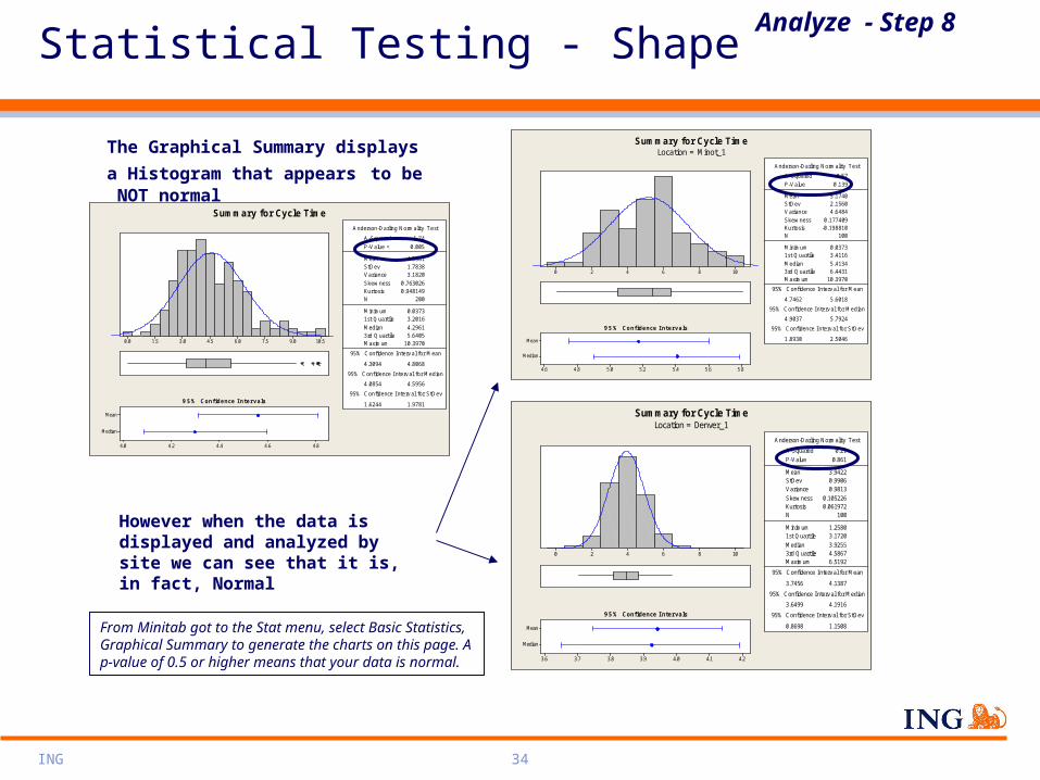
Statistical Testing - ShapeAnalyze - Step 8
The Graphical Summary displays a Histogram
that appears to be NOT normal
However when the data is displayed and analyzed by site we can see that it is, in fact, Normal
10.59.07.56.04.53.01.50.0
Median
Mean
4.84.64.44.24.0
Anderson-Darling Normality Test
Variance 3.1820Skewness 0.763026Kurtosis 0.948149N 200
Minimum 0.0373
A-Squared
1st Q uartile 3.2016Median 4.29613rd Q uartile 5.6405Maximum 10.3970
95% Confidence I nterval for Mean
4.3094
1.74
4.8068
95% Confidence I nterval for Median
4.0854 4.5956
95% Confidence I nterval for StDev
1.6244 1.9781
P-Value < 0.005
Mean 4.5581StDev 1.7838
95% Confidence I ntervals
Summary for Cycle Time
1086420
Median
Mean
5.85.65.45.25.04.84.6
Anderson-Darling Normality Test
Variance 4.6484
Skewness 0.177409Kurtosis -0.198810N 100
Minimum 0.0373
A -Squared
1st Q uartile 3.4116
Median 5.41343rd Q uartile 6.4431Maximum 10.3970
95% Confidence I nterval for Mean
4.7462
0.57
5.6018
95% Confidence I nterval for Median
4.9037 5.7924
95% Confidence I nterval for StDev
1.8930 2.5046
P-Value 0.139
Mean 5.1740StDev 2.1560
95% Confidence I ntervals
Summary for Cycle TimeLocation = Minot_1
1086420
Median
Mean
4.24.14.03.93.83.73.6
Anderson-Darling Normality Test
Variance 0.9813Skewness 0.105226Kurtosis 0.061972N 100
Minimum 1.2580
A-Squared
1st Quartile 3.1720Median 3.92553rd Quartile 4.5867Maximum 6.5192
95% Confidence Interval for Mean
3.7456
0.21
4.1387
95% Confidence Interval for Median
3.6499 4.1916
95% Confidence Interval for StDev
0.8698 1.1508
P-Value 0.861
Mean 3.9422StDev 0.9906
95% Confidence I ntervals
Summary for Cycle TimeLocation = Denver_1
From Minitab got to the Stat menu, select Basic Statistics, Graphical Summary to generate the charts on this page. A p-value of 0.5 or higher means that your data is normal.

ING 35
Statistical Testing – Hypothesis TestingAnalyze - Step 8
Now that you have charted the data and determined that there are 2 independent process Use Hypothesis Testing to determine if there is a Statistical Difference between them.
To do this we must first state our NULL HYPOTHESIS or (Ho) and our ALTERNATIVE HYPOTHESIS (Ha)
Ho = There IS NOT a statistical difference in cycle time for the Minot and Denver processing sites.
Ha = There IS a statistical difference in cycle time for the Minot and Denver processing sites.

ING 36
Analyze - Step 8
Input Data Type Normality Test Used Result of Test Variance
(p-value)
Variance Equal Result of Test Centering
(p-value)
Centering
Equal
Cycle time
(Y Response)
Continuous N/A N/A N/A N/A N/A N/A
Minot
(X Factor)
Discrete Normal Use the decision tree on next page Enter p-value from test N Enter p-value from test N
Denver
(X Factor)
Discrete Normal Use the decision tree on next page Enter p-value from test N Enter p-value from test N
Chi Square
X (Factor)
Y (
Res
po
nse
)
Continuous Discrete
Co
nti
nu
ou
sD
iscr
ete
Scatter plot Simple
Regression Multiple
Regression
T-tests ANOVA Probability Plot Test for Variance Mood’s Median
Logistic Regression
Chi Square
The Matrix above can serve as a quick reference to which tool (s) you can use depending on what type of data you have.
Statistical Testing – Hypothesis Testing

ING 37
Analyze - Step 8
C6
95% Bonferroni Confidence Intervals for StDevs
Minot
Denver
2.42.22.01.81.61.41.21.0
C6
Stacked
Minot
Denver
121086420
F-Test
0.000
Test Statistic 0.31P-Value 0.000
Levene's Test
Test Statistic 24.68P-Value
Test for Equal Variances for Stacked
Statistical Testing – Spread (Variance)
Based on the resultant p-value – 0.00, the variances are NOT equal
Test for Equal Variances: Cycle time vs. location
95% Bonferroni confidence intervals for standard deviations
C6 N Lower StDev Upper
Denver 100 0.96453 1.11872 1.32878
Minot 100 1.73295 2.00998 2.38739
F-Test (normal distribution)
Test statistic = 0.31, p-value = 0.000
Levene's Test (any continuous distribution)
Test statistic = 24.68, p-value = 0.000

ING 38
Analyze - Step 8Statistical Testing – Spread (Centering)
Based on the resultant p-value – 0.00, the centers are NOT equal.
There for we must reject the null Ho and accept the alternative Ha.
Ha = There IS a statistical difference in the variances (spread) of cycle time for the Minot and Denver processing sites.
Location
Sta
cked
MinotDenver
12
10
8
6
4
2
0
Boxplot of Stacked by Location
Location
Sta
cked
MinotDenver
12
10
8
6
4
2
0
Individual Value Plot of Stacked vs Location
Two-Sample T-Test and CI: Stacked, Location
Two-sample T for Stacked
Location N Mean StDev SE Mean
Denver 100 3.91 1.12 0.11
Minot 100 4.81 2.01 0.20
Difference = mu (Denver) - mu (Minot)
Estimate for difference: -0.898457
95% CI for difference: (-1.352886, -0.444028)
T-Test of difference = 0 (vs not =): T-Value = -3.91
P-Value = 0.000 DF = 154

ING 39
Evaluate Root Cause RelationshipsAnalyze - Step 9
projects
days
to p
lan
17.515.012.510.07.55.0
70
60
50
40
30
20
S 9.68761R-Sq 58.1%R-Sq(adj) 55.1%
Fitted Line Plotdays to plan = 11.22 + 3.441 projects
Residual
Perc
ent
20100-10-20
99
90
50
10
1
Fitted Value
Resi
dual
7060504030
20
10
0
-10
Residual
Fre
quency
20151050-5-10-15
3
2
1
0
Observation Order
Resi
dual
16151413121110987654321
20
10
0
-10
Normal Probability Plot of the Residuals Residuals Versus the Fitted Values
Histogram of the Residuals Residuals Versus the Order of the Data
Residual Plots for days to plan
Fitted Line Chart with Regression
Potential Root Causes of your Defect:• Use Scatter Plots, Fitted Line Plots and Regression
Plots to determine the strength of the relationship between the sources of variation

ING 40
Preliminary Cost Benefit Analysis (CBA)Analyze - Step 9
Double Click on the CBA Icon to Launch
Copy and Paste Summary ReportCBA Sheet

ING 41
Summarize findings, present recommendations and document next steps.
Next Steps

ING 42
• Baseline• Calculate the current Sigma level
• Establish Baseline
• Statistical Analysis• Chart the Stability of your data
• Run Chart
• Control Charts
• Chart the Shape of your data• Graphical Summary
• Histograms
• Pareto Charts
• Establish the Null and Alternative Hypothesis’s
• Document your Y and your X’s• Determine your data type
• Use the Statistical Road map to select the appropriate tests for your data type• DISCRETE Data
• Chi Squared Test• CONTINIOUS Data
• Analyze the variance of your data• Analyze the centering of your data
• State the results of the testing and accept or reject the Null Hypothesis
• Populate the Fishbone to identity sources of variation
• Preliminary Cost Benefit Analysis• CBA Template Completed and signed off
• Project Schedule Updated
• Documented NEXT Steps for Improve
• Project Meeting Completed• Review Analyze material and Prep for tollgate
Analyze Tollgate Checklist

ING 43
Improve - Step 10
* Note: Fill out only the fields that are shaded greenAlternatives
Key Criteria Imp
ort
ance
Rat
ing
Ben
chm
ark
Op
tio
n
Alt
ern
ativ
e 1
Alt
ern
ativ
e 2
Alt
ern
ativ
e 3
Criteria 1Criteria 2
Sum of Positives 0 0 0Sum of Negatives 0 0 0Sum of Sames 0 0 0Weighted Sum of Positives 0 0 0Weighted Sum of Negatives 0 0 0
Concept Selection LegendBetter +Same SWorse -
Which alternative improvement works best for you? Why?
<Input Alternative that was selected HERE. State what made it stand out as the best solution.>
Pugh Matrix
Develop Improvements

ING 44
Improve - Step 10Design of Experiment - DOE
DOE

ING 45
Improve - Step 10
1
3 4
2
High Low
Easy
Hard
Imp
lem
en
tati
on
Which Option works best for you? Why?
<Enter the name of the best improvement option and briefly describe why it fits into the category that you selected>
ImpactImpact / Effort MatrixAction Workout 4-Blocker:
1 – high impact, easy to do
2 – low impact, easy to do
3 – high impact, not so easy to do
4 – low impact, not so easy to do
Develop Improvements
ING 46
PFD – Improved Process Flow Diagram Improve - Step 10
Insert your Improved Process map here
Indicate steps that were changed or deleted.Identify re-work loops that were removed or improvedIf possible show improved cycle times or decreased volumes

ING 47
Failure Modes and Effect AnalysisImprove - Step 10
Actions Taken Ne
w S
EV
Ne
w P
RO
B
Ne
w D
ET
Ne
w R
PN
Process Step that could fail
Reasons that the failure could occur
Effects of the failure
What would cause the step to fail?
What are we currently doing to prevent failure? 0
What should we do so that the step does not fail as often, is not as severe, or is easier to detect?
Who will implement the fixes and what is the target date?
What actions have been taken? 1 2 1 2
0
0
0
0
0
0
0
0
0
0
0
Item/Function
Potential Failure Modes
Potential Effects of Failure
S
E
V
Potential Causes of
Failure
P
R
O
B
Current Design
Controls
D
E
T RPN
Recommended Actions
Target Date and
Responsibility
Action Results
FMEA
See Instructions in Appendix

ING 48
Pilot SolutionImprove - Step 11
Objectives
1. (e.g., determine user acceptance, test with customer...)
2. (e.g., evaluate cycle time reduction, increase in accuracy...)
Method: (1-2 sentence description of sample size, extent of testing)
(1-2 sentence description of communication plan)
(1-2 sentence description of training plan)
Pilot Solution
Communicate Solution
Train Users / Processors

ING 49
Pilot ResultsImprove - Step 10
App Rec to Policy Mailed Days
Nu
mb
er
of
Ca
ses
1501209060300
80
70
60
50
40
30
20
10
0
Normal Old Process Vs. New Process (App Received to Policy Issued)

ING 50
Summarize findings, present recommendations and document next steps.
Next Steps

ING 51
• Evaluate Multiple Solutions• Pugh Matrix• Effort Impact Matrix• DOE
• Process Flow Diagram• Completed and Validated
• Complete and Validate FMEA
• Identify and Evaluate Risks• Complete and Validate FMEA
• Prepare Necessary Training Material
• Pilot Solution
• Project Schedule Updated
• Documented NEXT Steps for Control
• Project Meeting Completed• Review Improve material and Prep for tollgate
Improve Tollgate Checklist

ING 52
Validate Measurement System (X’s)Control - Step 12
HowWhatPurpose of CollectionData TypeMeasure Type
Measures
Operational Definitions and Procedures
Clarify Data Collection Goals
How ManyWhoWhenWhereWhat
Operational Procedures for Collection and Recording
Method of Validating Measurement System Segmentation Factors

ING 53
Per
cent
Part-to-PartReprodRepeatGage R&R
100
50
0
% Contribution
% Study Var
Sam
ple
Ran
ge
1.0
0.5
0.0
_R=0.342
UCL=0.880
LCL=0
A B C
Sam
ple
Mea
n
2
0
-2
__X=0.001UCL=0.351LCL=-0.348
A B C
Part10987654321
2
0
-2
OperatorCBA
2
0
-2
Part
Ave
rage
10 9 8 7 6 5 4 3 2 1
2
0
-2
Operator
A
BC
Gage name:Date of study:
Reported by:Tolerance:Misc:
Components of Variation
R Chart by Operator
Xbar Chart by Operator
Measurement by Part
Measurement by Operator
Operator * Part Interaction
Gage R&R (ANOVA) for Measurement
Continuous Data Gage R&R
Validate Measurement SystemControl – Step 12

ING 54
Measurement System Analysis (MSA)Control - Step 12
Discrete Data Gage R&R
Statistical Report - Discrete Data Analysis Method
DATE: 01/00/1900NAME: 01/00/1900
PRODUCT: 01/00/1900BUSINESS: 01/00/1900
Repeatability AccuracySource Dave Dawn 0 Dave Dawn 0Total Inspected 0 0 0 0 0 0# Matched 0 0 0 0 0 0False Positives 0 0 0False Negatives 0 0 0Mixed 0 0 095% UCL #DIV/0! #DIV/0! #DIV/0! #DIV/0! #DIV/0! #DIV/0!Calculated Score #DIV/0! #DIV/0! #DIV/0! #DIV/0! #DIV/0! #DIV/0!95% LCL #DIV/0! #DIV/0! #DIV/0! #DIV/0! #DIV/0! #DIV/0!
Overall Repeat. and Reprod. Overall Repeat., Reprod., & AccuracyTotal Inspected 0 0# in Agreement 0 095% UCL #DIV/0! #DIV/0!Calculated Score #DIV/0! #DIV/0!95% LCL #DIV/0! #DIV/0!
Repeatability by Individual
0.0%10.0%20.0%30.0%40.0%50.0%60.0%70.0%80.0%90.0%
100.0%110.0%
Dave Dawn 0
Rep
eata
bil
ity
95% UCLCalculated Score95% LCL
Accuracy by Individual
0.0%10.0%20.0%30.0%40.0%50.0%60.0%70.0%80.0%90.0%
100.0%110.0%
Dave Dawn 0
Acc
ura
cy
95% UCLCalculated Score95% LCL
Microsoft Excel Worksheet
Double Click on the Excel Icon to Launch the
Discrete Data Analysis Tool
Copy and Paste Summary Report

ING 55
Establish New Process Capability
Baseline Process Capability – Discrete Data
(DPMO Calculation)
Control - Step 13
Baseline Process Capability – Continuous Data
(Process Report from Minitab)
10.59.07.56.04.53.01.50.0
LSL Target USLProcess Data
Sample N 200StDev(Within) 1.67987StDev(O verall) 1.78605
LSL 2Target 5USL 10Sample Mean 4.5581
Potential (Within) Capability
Cpk 0.51Lower CL 0.44Upper CL 0.58
O verall Capability
Z.Bench 1.42Lower CL
Z.Bench
1.16Z.LSL 1.43Z.USL 3.05Ppk 0.48Lower CL 0.41Upper CL
1.52
0.54Cpm 0.54Lower CL 0.50
Lower CL 1.25Z.LSL 1.52Z.USL 3.24
O bserved PerformancePPM < LSL 50000.00PPM > USL 15000.00PPM Total 65000.00
Exp. Within PerformancePPM < LSL 63904.64PPM > USL 598.75PPM Total 64503.39
Exp. O verall PerformancePPM < LSL 76033.76PPM > USL 1156.13PPM Total 77189.89
WithinOverall
Process Capability of Cycle Time(using 95.0% confidence)
Calculating Process Sigma for Discrete Data
enter 1 Number Of Units Processed N= 246
2 Total Number Of Defects Made (Include Defects Made And Later Fixed) D= 45
3 Number Of Defect Opportunities Per Unit O= 3
4 Solve For Defects Per Million Opportunities 60976
5 Look Up Process Sigma In Abridged Sigma Conversion Table Sigma= 3.05
Units =
Defects =
Opportunities =
DPMO =
Baseline Sigma =

ING 56
Assess New Process Capability
Baseline (Before Project)
New (After Project)
Sigma DPMO
1.42
3
<>
<>
Before and After Performance Assessment
Control - Step 13
Validate Statistical Improvement
H0=There is no difference between the baseline and the new Process Capability
HA = There is a difference between the baseline and the new Process Capability
If P > .05 there is no difference between the Processes
If P < .05 there is a difference between the Processes
Chi-Square Test: defects, units, opps
defects units opps Total 1 1245 10000 2 11247 866.59 10378.33 2.08 165.238 13.792 0.003
2 425 10000 2 10427 803.41 9621.67 1.92 178.232 14.876 0.003
Total 1670 20000 4 21674
Chi-Sq = 372.144, DF = 2, P-Value = 0.0002 cells with expected counts less than 5.
Validate Statistical Improvement

ING 57
Final Cost Benefit Analysis (CBA)Control - Step 14
Copy and Paste the Updated
CBA File from Analyze Step 9
CBA Sheet

ING 58
Control Chart SelectionControl Chart Selection
Implement Process Control – Chose a Control Chart
Control - Step 14
Data Type?
Type of Discrete Data?
Constant Sample Size? Constant Opportunity?Sample Size< 10
Individual Measurements
OrSub-Groups
DISCRETE
Individual and Moving Range
ChartX and R Chart X and S Chart P Chart NP Chart C Chart U Chart
CONTINUOUS
NOYES YES NO
NOYES
RATIONALSUB GROUPSINDIVIDUALS

ING 59
0Subgroup 1 2 3 4 5 6 7 8 9 10
0
10
20
Indi
vidu
al V
alue
X=10.00
3.0SL=19.16
-3.0SL=0.8392
0
5
10
Mov
ing
Ran
ge
1
R=3.444
3.0SL=11.25
-3.0SL=0.00E+00
I and MR Chart for Avg Cycle ti
Control ChartControl Chart
Key Drivers (X’s) Measurement Continuous or Discrete
<From Step 7> <How will you measure the x?> Continuous or Discrete?
<From Step 7> <How will you measure the x?> Continuous or Discrete?
<From Step 7> <How will you measure the x?> Continuous or Discrete?
Implement Process Control
Ongoing Measurement Plan
Control - Step 14
Insert the appropriate
control chart as indicated on the previous slide

ING 60
Stakeholders Map – Pre ImprovementControl - Step 14
* When Populating the Stakeholder, consider the FAST Method• F= FYI – Information Only• A= Approver• S= SME Subject Matter Expert• T= Team Member
Infl
uen
ce O
n P
roje
ct
Hig
hM
ediu
mL
ow
Low Medium HighImpacted By Project
StakeholderPosition
StronglySupportive
Neutral
Opponent
1S2S
3F
4T
5A
6F
7A
8S 9S
10A
11T
Stakeholders: Distribution, New Business, Underwriting,
Legal, IT, Actuary, Web Team, Customer Svc/Ops, Marketing, Finance, Compliance
Where are your Stakeholders NOW ?

ING 61
Turnover to the BusinessTurnover to the Business
• Has the business agreed to accept this process? <YES or NO>• Who owns the new process? <Name & Role of the person or department>• Who runs the new process? <Name & Role of the person or department>• Has this person(s) been properly trained? <YES or NO>• Who monitors the new process and metrics? <Name of the person or department>• What would happen if you were not available? <Is there an FMEA to aid in troubleshooting?>
Where else can the new process owner get support?
DocumentationDocumentation
• What kind of documentation is available? <e.g. Checklist, Manual, Improved Process Map>• Where is the documentation located? <specifically describe the location, e.g. drive
mapping>• Who has access to the information? <Names of people or department>• Who will be responsible for updating the information? <Names of people or department>• How is documentation / file change control managed? <How is documentation protected from
unauthorized changes?>
Implement Process ControlControl - Step 14

ING 62
Control Tollgate Checklist
• Measurement System Analysis • Gage R&R or DDA
• Calculate New Process Capability• Calculate the current Sigma Level
• Evaluate Project Results• Compare Baseline and New Sigma Levels• Statically Validate Improvement• Establish the Null and Alternative Hypothesis’s
• Final Cost Benefit Analysis• CBA Template Completed and signed off
• Document ongoing measures
• Chart Control Data• Use appropriate Control Chart (s)
• Complete Project Documentation
• Turn Process Over to the Business
• Project Meeting Completed• Review Control material and Prep for tollgate
• Hold Final Project Tollgate and Celebrate Success !!!!

ING 63
APPENDIX APPENDIX
• Key Deliverables
• FMEA Scoring Guidelines
• Sample Team / Tollgate Meeting Agenda

ING 64
We
ek
1
We
ek
2
We
ek
3
We
ek
4
We
ek
5
We
ek
6
We
ek
7
We
ek
8
We
ek
9
We
ek
10
We
ek
11
We
ek
12
We
ek
13
We
ek
14
We
ek
15
We
ek
16
DEFINE
- Develop Team Project Plan
- Develop Team Charter
- Identify Customer and Customer Requirements
- Identify and Validate Business Opportunity
- Define Business Process
- Quantify Financials
- Conduct Define Tollgate
MEASURE
- Identify and Select Metrics / Indicators
- Develop Operational Definitions
- Determine Performance Standards
- Develop Data Collection Plan
- Validate Measurement System
- Collect and Analyze Data
- Conduct Measure Tollgate
ANALYZE
- Assess Current Process Capability and Performance
Identify stastical goal (Sigma or DPMO Improvement)
- Identify Potential Root Cause(s)
- Stratify the Data and Identify Specific Problem(s)
- Determine Sources of Variation
- Collect and Analyze Data
- Validate Root Cause(s)
- Conduct Analyze Tollgate
IMPROVE
- Brainstorm Solution Ideas
- Determine Process and Financial Benefits
- Develop a Proposed Solution
- Develop Pilot Plan and Pilot Solution
- Assess Pilot Solution Capability and Performance
- Refine (if needed) and Document New Process
- Conduct Improve Tollgate
CONTROL
- Define and Validate Measurement System
- Collect and Analyze Data
- Assess New Process Capability and Performance
- Validate Improvement Goal Achieved
- Develop and Implement Process Control Plan
- Conduct Control Tollgate
Key DeliverablesAPPENDIX

ING 65
Severity Rating Scale: The Severity of a failure should it occur
Occurrence Rating Scale: The Likelihood or Frequency of Failure
Detection Rating Scale: The likelihood of a failure being Detected before its effect is realized
BAD 10 Injure a customer or employee More than once per day (>30%) Defect Caused by failure is not detectable
9 Be Illegal / Cause Controllership Issues Once every 3-4 days(<= 30%)
Occasional units are checked for defects
8 Render the product or service unfit for use Once per week(<=5%)
Units are systematically sampled and inspected
7 Cause extreme customer dissatisfaction Once per month(<=1%)
All units are manually inspected
6 Result in partial malfunction Once every 3 months (<=.03%) Units are manually inspected with mistake-proofing modifications
5 Cause a loss of performance which is likely to result in a complaint
Once every 6 months (<= 1 per 10,000)
Process is monitored (SPC) and manually inspected
4 Cause a minor performance loss Once per year(<= 6 per 100,00)
SPC is used with an immediate reaction to out of control conditions
3 Cause a minor nuisance but be overcome with no performance loss
Once every 1-3 years (<= 3 per million
SPC as above with 100% inspection surrounding out of control conditions
2 Be unnoticed and have only minor effect on performance
Once every 3-6 years (<=3 per 10 million)
All units are automatically inspected
GOOD 1 Be unnoticed and not affect the performance Once every 6-100 years (<=2 per billion)
Defect is obvious and can be kept from affecting the customer
FMEA Scoring GuidelinesAPPENDIX

ING 66
Sample Team Meeting / Tollgate AgendaAPPENDIX
Six Sigma Kick-Off for Life Licensing & Contracting June 28, 2005
Location: 6A North Conference Room Des Moines, IA Dial In: 866-464-6338 (participant code 62805) Attire: Business Casual Time Topic Led By Tuesday, June 28 10:00 – 10:15 am Introductions and Opening Remarks Chris Fleming, Jackie Figliola
10:15 – 10:45 am Six Sigma Overview, Roles &
Responsibilities Jim Cottone, Stacy Bagby
10:45 – 11:30 am Review Project Charter and Project Scope Jim Cottone, Stacy Bagby
11:30 – 12:15 pm Validate Voice of Customer, Voice of Business
Jim Cottone, Stacy Bagby
12:15 – 12:30 pm Break
12:30 pm Working Lunch 6A North
12:30 – 2:15 pm Review and Validate SIPOC & High-Level Process Flow
Jim Cottone, Stacy Bagby
2:15 – 2:30 pm Break
2:30 – 3:15 pm Current and Future Measurements Jim Cottone, Stacy Bagby
3:15 – 4:00 pm Develop Project Schedule Jim Cottone, Stacy Bagby
4:00 – 5:00 pm Lessons Learned, Next Steps and Wrap Up Chris Fleming, Jim Cottone, Stacy Bagby
5:00 pm Adjourn, Departures
Additional Information Lunch, refreshments and snacks will be provided throughout the day. Hard copies of all documents will be made available to all meeting participants.
You can double click on the form to launch the word document.
Modify the content as necessary for your project